This PDF is a selection from an out-of-print volume from the National Bureauof Economic Research

Volume Title: Developing Country Debt and Economic Performance, Volume3: Country Studies - Indonesia, Korea, Philippines, Turkey

Volume Author/Editor: Jeffrey D. Sachs and Susan M. Collins, editors

Volume Publisher: University of Chicago Press

Volume ISBN: 0-226-30455-8

Volume URL: http://www.nber.org/books/sach89-2

Conference Date: September 21-23, 1987

Publication Date: 1989

Chapter Title: Savings and Investment

Chapter Author: Susan M. Collins, Won-Am Park

Chapter URL: http://www.nber.org/chapters/c9038

Chapter pages in book: (p. 234 - 249)

234 Susan M. Collins and Won-Am Park

Table 7.12 Percentage Changes in Components of Import Growth, 1977-85

Year Import Value Import Volume Unit Value Real GNP

1977 1978 1979 1980 1981 I982 1983 1984 1985

23.2 38.5 35.8 9.6

17.2

8.0 16.9 1.6

-7.2

20.5 31.2 11.1

-8.9 11.2 2.2

13.3 15.4 6.2

2.2 5.6

22.2 20.3 5.4

-7.4 -4.7

1.3 -4.2

10.7 11.0 7.0

-4.8 6.6 5.4

11.9 8.5 5.4

8 Savings and Investment

During each of Korea’s periods of rapid debt accumulation, virtually all of the additional foreign borrowing was used to finance current account deficits. Since domestic investment must be financed through some combination of domestic and foreign savings, foreign savings-r the deficit in the current account-is exactly equal to the imbalance between domestic savings and investment.

In this chapter we examine the behavior of the current account from the savings-investment perspective. The decomposition is especially interesting for Korea because its experience differs markedly from that of many other debtor countries. A frequently observed pattern is for the current account deficit to increase as government savings decline and then for a current account improvement to be attained, at least in the short run, through cuts in (public and private) investment and in government expenditure, thus raising government savings. Relatively little of the adjustment tends to be achieved through private sector savings.

Korean experience contrasts with the “stylized” scenario with respect to the roles of investment, public savings, and private savings. First, fiscal deficits have played at most a minor role in current account deterioration. Instead, increases in fixed investment, associated with new economic development strategies, have outpaced rising private savings. This leaves the door open for a jump in required foreign financing to cover either unexpected surges in inventory accumulation or unexpected drops in private savings. The series of five-year economic and social plans have played a critical role through their impact on investment. Second, the reduction of the current account deficit during the recovery is achieved without a substantial decline

235 KoredChapter 8

in investment. The adjustment comes from increased domestic savings, the lion's share of which is generated by the household sector.

This pattern is illustrated by figure 8.1. The plot shows the behavior of gross fixed investment and of domestic savings less inventory accumulation, each as a share of GNP. Accounting identities imply that the difference between these two variables is equal to the current account. When fixed investment is larger than the excess of domestic savings over inventory accumulation, the current account is in deficit, while small investment relative to the adjusted domestic savings is the counterpart of current account

In broad terms, fixed investment has behaved like a step function with rapid increases during 1965-68 and jumps in 1974 and 1979. There has been considerably more variation in the adjusted savings variable. The large current account deficits during 1970-71, 1974-75, and 1980-81 follow rises in fixed investment, but are precipitated primarily by reduced savings and/or increased inventories. Similarly, the current account improvements are explained by increased domestic savings relative to inventory accumula- tion, with only a small role for reduced fixed investment.

The remaining sections of the chapter examine savings and investment behavior in more detail. We turn first to domestic savings in section 8.1, and then to investment and the role of the five-year plans in section 8.2. The data used in this chapter are based on the old System of National Accounts (SNA) decomposition. This allowed a long enough time series for the empirical

surplus.

IF/GNP - (Sav-InvVGNP -.-.-. .35

.30 -

' l o - 66 ' L8 I 7b I i!2 I l'4 ' 76 I i!8 I i 0 I i 2 I 84

Year

IF = Gross Fixed Investment Inv = Accumulation of Stocks Sav= Domestic Savings

Fig. 8.1 Current account imbalance: ratios of investment and savings to GNP

236 Susan M. Collins and Won-Am Park

estimates. Furthermore, the new SNA data required to decompose domestic savings were only available for a few years at the time of this analysis. The data and the methods used for disaggregation are described in section 8.3.

8.1 Domestic Savings

In table 8.1 we show the behavior of domestic savings, foreign savings, and investment from 1965 to 1984. The top panel gives the variables in levels, while the bottom takes each variable relative to GNP. Evident from the table is the rise in savings from less than 15 percent of GNP during the mid-1960s to nearly 30 percent by the end of the 1970s. Also clear is that this impressive growth has been interrupted by drops of as much as 6 percent from one year to the next. Three sources of domestic savings are also identified: general government, public and private corporations, and other (including households and unincorporated businesses). Unfortunately, it is not possible to break the components down more finely.

The data show there has been a significant shift from government and corporations to households as a source of savings. In 1965 government savings constituted nearly half of the total, with household and other savings the smallest component, accounting for less than 18 percent of the total. By 1984 household savings had grown to nearly 45 percent of the total. The share of corporate savings was 27 percent, representing a drop of 10 percent. The contribution of government savings had fallen even more, also accounting for about 28 percent of the total by 1984.

Figure 8.2 shows government, corporate, and household savings relative to GNP during 1965-84. The three series have behaved quite differently. With the exception of the permanent increase in 1972, corporate savings have remained relatively flat, declining only slightly during economic downturns. One explanation for the increase in 1972 is the impact of the financial crisis and the August Emergency Decree, which effectively caused a transfer from lenders in the unofficial money market (UMM) to borrowers. The measure thereby succeeded in significantly reducing the activities of the UMM during the next year, nearly eliminating an important source of corporate finance. The transfer and the tighter access to funds would both be expected to increase corporate savings. Cole and Park (1983, 167) argue that any effects of the decree were short-lived, however, there does seem to have been a sustained effect on corporate savings. Corporate savings averaged 0.053 percent of GNP from 1965 to 1971 and, excluding the jump to 0.09 percent during 1972, averaged 0.075 percent during 1973-85.

Government savings have fluctuated more than corporate savings, but have been considerably less variable than household savings. The graph in figure 8.2 documents a small rise from 1967 to 1970, a decline during 1971-75, and a gradual return to government saving rates on the order of 6 percent of

Table 8.1 Domestic Savings by Source, 1965-84

Domestic Savings Current Gross Investment Account Statistical

Year Total Government Corporate Other Deficit Discrepancy Total Fixed Stocks

Panel A (in billions of won)

1965 113.30 51.90 1966 182.40 61.60 1967 206.70 89.00 1968 311.90 134.20 1969 476.80 157.40 1970 487.00 201.60 1971 550.70 198.50 1972 753.90 163.40 1973 1,301.10 231.00 1974 1,582.80 219.80 1975 2,037.10 407.90 1976 3.480.00 880.70 1977 5,087.80 974.40 1978 7,122.50 1,554.70 1979 8,993.80 2,185.90 1980 8,405.00 2,196.10 1981 10,260.60 2,915.10 1982 11,960.00 3,235.00 1983 14,974.90 4,495.00 1984 18.298.30 5,144.40

41.90 53.50 68.10 93.80

121.40 132.50 157.10 357.00 442.90 619.10 719.90

1,058.70 1,469.60 1,779.70 2,288.10 2,943.80 3,201 .SO 3,719.70 4,404.40 4,998.40

19.50 67.30 49.50 83.90

198.00 152.80 195.10 357.00 627.10 743.90 909.30

1,540.60 2,643.90 3,788. LO 4,519.80 3,265.10 4,143.70 5,004.90 6,075.40 8,155.60

- 2.40 28.10 51.90

121.80 158.20 193.50 294.70 144.60 123.20 820.40 913.20 151.80 -6.00 525.30

2,009.10 3,224.30 3,164.70 1,945.00 1,220.50 1,094.50

10.00 13.50 22.10

-6.00 - 13.60

12.80 2.70

24.40

-28.30 79.70

-74.80 -55.40 - 92.90 136.40

0.90 -82.30

66.30 30.00 54.70

-43.10

120.90 223.90 280.70 427.70 621.30 693.20 848.10 923.00

I ,38 I . 20 2,374.80 3,030.10 3,556.90 5,026.50 7,554.90

I I , 139.40 11.630.20 13.343.00 13,979.80 16,225.40 19,447.60

119.00 1.90 209.80 14.10 274.60 6.10 413.60 14.10 555.80 65.50 627.10 66.10 726.40 121.70 830.80 92.20

1,257.70 123.50 I ,898.80 476.00 2,573.40 456.70 3,343.30 213.60 4,830.00 196.50 7,463.60 91.30

899.70 10,239.70 11,873.90 -243.70 13,208.10 134.90 15,675.60 - 1,695.80 18,604.80 -2,379.40 20,175.50 -727.90

(continued)

Table 8.1 (continued)

Domestic Savings Current Gross Investment Statistical Account

Year Total Government Corporate Other Deficit Discrepancy Total Fixed Stocks

Panel B (in percentage of GNP)

I965 14.06 6.44 5.20 2.42 -0.30 1.24 15.01 14.77 0.24 I966 17.59 5.94 5.16 6.49 2.71 1.30 21.59 20.23 1.36 1967 16.13 6.95 5.32 3.86 4.05 1.72 21.91 21.43 0.48 1968 18.87 8.12 5.67 5.08 7.37 -0.36 25.88 25.02 0.85 1969 22.12 7.30 5.63 9.19 1.34 - 0.63 28.83 25.79 3.04 1970 17.68 7.32 4.81 5.55 7.03 0.46 25.17 22.77 2.40 1971 16.32 5.88 4.65 5.78 8.73 0.08 25.13 21.52 3.61 1972 18. I5 3.93 8.59 8.59 3.48 0.59 22.22 20.00 2.22 1973 24.19 4.29 8.23 11.66 2.29 -0.80 25.68 23.38 2.30 1974 21.10 2.93 8.25 9.91 10.93 -0.38 31.65 25.31 6.34 1975 20.18 4.04 7.13 9.01 9.05 0.79 30.02 25.50 4.53 1976 25.07 6.34 7.63 11.10 1.09 -0.54 25.62 24.09 1.54 1977 28.09 5.38 8.11 14.59 -0.03 -0.31 27.75 26.66 I .08 1978 29.40 6.42 7.35 15.64 2.17 -0.38 31.19 30.81 0.38 1979 28.78 7.00 7.32 14.46 6.43 0.44 35.65 32.17 2.88 1980 22.92 5.99 8.03 1981 22.74 6.46 7.10 9.18 7.01 -0.18 29.57 29.27 0.30 1982 23.58 6.38 7.33 9.87 3.83 0.13 27.56 30.90 -3.34 1983 25.39 7.62 7.41 10.30 2.07 0.05 27.51 31.54 -4.03 1984 27.55 7.75 7.53 12.28 1.65 0.08 29.28 30.38 -1.10

8.90 8.79 0.00 31.71 32.38 -0.66

Source: EPB, Major Statistics of Korean Economy, 1986, and BOK, Flow of Funds Statistics, 1984.

Note: Statistical Discrepancy is the difference between the depreciation allowance from the two sources (see discussion in sec. 8.3).

239 KoredChapter 8

Household Savings ---- Government Savings - Corporate Savings

I SAVl NGS/GNP 17.5

Fig. 8.2 Components of savings/GNP

GNP. It also provides some evidence for an inverse relationship between government and household savings, particularly during the mid- 1970s.

We turn next to an analysis of household savings, the most variable and, since 1972, the largest component of domestic savings. There are two facts to be explained. First, how did Korea managed to triple household saving rates from 5 percent during 1966-68 to 15 percent during 1977-79? And second, why have there been such large fluctuations in the household saving rate?

Household savings are computed as the difference between domestic savings and the sum of general government and corporate savings. As already mentioned, they also include the savings of unincorporated businesses. Therefore, part of this component is a capital consumption allowance. Table 8.2 divides household savings into depreciation (HSD) and other (HSO). Not surprisingly, the depreciation has been quite stable as a share of GNP, ranging from 2.0 to 2.7 percent. Movements in this component clearly cannot explain the large fluctuations in the total.

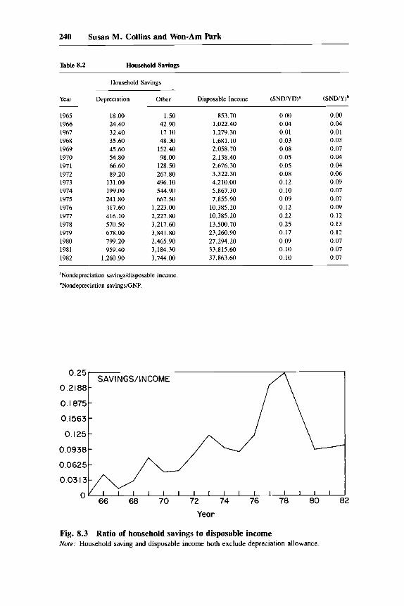
Figure 8.3 plots the ratio of household savings excluding depreciation to disposable personal income (HSOIYD). It shows that savings have risen relative to income in a ratchet fashion, which is suggestive of a permanent income model of consumption. In such a model, temporary and unexpected rises in income will have a relatively small affect on consumption, leading to short-run jumps in savings. The model seems particularly relevant for the Korean economy with its periodic growth spurts and slowdowns.

Another factor which may help to explain the large fluctuations in savings is the real interest rate. Some authors have argued that increases in interest

240 Susan M. Collins and Won-Am Park

Table 8.2 Household Savings ~

Household Savings

Year Depreciation Other Disposable Income (SND/YD)" (SND/Y)b

1965 18.00 1 S O 853.70 0.00 0.00 1966 24.40 42.90 1,022.40 0.04 0.04 1967 32.40 17.10 1,279.30 0.01 0.01 1968 35.60 48.30 I,681.10 0.03 0.03 1969 45.60 152.40 2,058.70 0.08 0.07 1970 54.80 98.00 2,138.40 0.05 0.04 1971 66.60 128.50 2,676.30 0.05 0.04 1972 89.20 267.80 3,322.30 0.08 0.06 1973 131.00 496.10 4,210.00 0.12 0.09 1974 199.00 544.90 5,867.30 0.10 0.07 1975 241 .SO 667.50 7,855.90 0.09 0.07 1976 317.60 1,223.00 10,385.20 0.12 0.09 1977 416.10 2,227.80 10,385.20 0.22 0.12 1978 570.50 3,217.60 13,500.70 0.25 0.13 1979 678.00 3,84 I . 80 23,260.90 0.17 0.12 1980 799.20 2,465.90 27,294.20 0.09 0.07 1981 959.40 3,184.30 33.815.60 0.10 0.07 1982 1,260.90 3,744.00 37,863.60 0.10 0.07

"Nondepreciation sdvings/disposable income.

bNondepreciation savingsiGNP.

0.25-

0.2 I88 - 0.1875-

0.1563 - 0.125-

0.0938 - 0.0625 - 0.0313-

SAVINGS/INCOME

Year

Fig. 8.3 Ratio of household savings to disposable income Note: Household saving and disposable income both exclude depreciation allowance.

241 KoredChapter 8

rates relative to inflation generate additional savings and that financial reform in 1965 was the key to understanding the jump in Korean saving rates during the mid-1960s.' Giovannini (1983) and others have found little sensitivity of saving to interest rates in empirical studies of a broad sample of developing countries. Thus, it is interesting to examine the relationship between saving and interest rates for the more recent period, 1965-82. Korean bank deposits have been adjusted a number of times during this interval, but adjustments have typically not kept pace with inflation, leading to substantial variation in real interest rates.

We assume a simple structure to explain saving behavior. Consumption is assumed to depend positively on income and negatively on the real return to saving. The consumption function, given by equation ( I ) , allows for different marginal propensities to consume out of permanent and transitory incomes. Equation (2) state that household savings are identically equal to disposable income less consumption. Disposable income is taken net of depreciation, so that the structure determines only the determinants of nondepreciation savings.

(1) C = O L ~ + (YIYP i O L ~ Y ~ ' + a3RR + E (2) HSO = YD - C

where YD = YP + YT = Y - T - HSD; Y is personal income; YD is personal disposable income, less depreciation; YP and YT are (perceived) permanent and transitory income; C is household consumption; RR is the real interest rate; and HSO and HSD are the depreciation and nondepreciation savings.

Temporary and permanent income were established as follows. Disposable income in period t was estimated as a linear function of disposable income from periods t - 1 and t - 2. Permanent income was measured as the fitted values from this regression while residuals were taken as a measure of transitory income. Using this procedure, transitory income ranged from 2 percent to nearly 10 percent of total disposable income. As expected, transitory income is very large and negative during 1970, 1980, and 1982. It is large and positive during 1974, 1978, and 1981. We use the nominal interest rate on one-year time deposits, deflated by the CPI. Other specifications, for example the use of curb market interest rates, did not significantly alter the estimation results.

The estimation results from equation (1) are given below in equation (3), with t-statistics in parentheses. They very strongly support a permanent- temporary income model for Korean consumption behavior.

(3) C = 91.20 + 0.88 YP + 0.55 YT - 16.50 RR (0.44) (77.62) (4.26) (-0.95)

Sample: 1965-82; adjusted R2 = 0.98; Durbin Watson = 1.78.

242 Susan M. Collins and Won-Am Park

They show a marginal propensity to consume out of permanent income of 0.88. The marginal propensity to consume out of temporary income is significantly smaller, 0.55. The estimates for the constant term and the influence of the real interest rate, however, are measured imprecisely and are not significantly different from zero.

The regression does not provide support for the view that changes in real interest rates have been a critical determinant of saving behavior. Instead, it emphasizes the importance of the high average growth of disposable income as an explanation for the impressive rise in household savings, and the large swings in real growth rates as an explanation for the cyclic fluctuations in saving rates. However, the very dramatic rise in Korean household savings is unusual and has played an important part in Korea’s successful adjustment. Korean saving behavior clearly warrants additional analysis.

8.2 Investment

8.2.1 Trends in Fixed Capital Formation

We begin with a discussion of the general trends in gross investment, focusing on the behavior of fixed capital formation. As already mentioned, and as illustrated in Figure 8.1, investment as a share of income follows cycles which coincide with the five-year development plans. In the first or second year of each plan, there has been a sudden rise in fixed capital formation. The increases continue through the third or fourth year of the plan and taper off somewhat in the last one to two years.

The main thrust of each five-year plan is summarized in table 8.3. In table 8.4 we summarize the shares of gross domestic capital formation by industry and by type of capital good during 1972-84. This period includes the third, fourth, and original fifth five-year plans. The major developments during each plan period do in fact coincide with the stated plan objectives.

During the third plan, 1972-76, and particularly during 1972-74, there was an increase in allocation to agriculture. Most of this increase came from declines in allocation to social overhead capital-transportation, storage, and communication. However, this sector retained the largest share of total investment, with manufacturing a close second.

During the fourth plan there was a decline in the share of investment in agriculture. Allocation to manufacturing and social overhead also fell, with services growing substantially (especially wholesale and retail trade and public administration). The decline in manufacturing occurred during the 1980-81 retrenchment from the Big Push. During 1977-81, over 77 percent of investment in equipment in manufacturing went to the HC industries. It is also interesting that equipment, as a share of investment, jumped from 31 to

243 KoredChapter 8

Table 8.3 Main Focus of Five-Year Plans

First plan (1962-66)

Second plan (1967-71)

Third plan (1972-76)

Fourth plan (1977-81)

Fifth plan Original (1982-86)

Revised (1984- 86)

Emphasis on basic industries for import substitution and expansion of social overhead capital

Export-oriented industrialization to promote labor-intensive light manufacturing

Development of rural sector-balanced economic growth and stability Deepening industrial structure through promotion of HC industries

Initially-continued push toward HC industries From 1978/7%shift toward industrial restructuring and price stabilization

Priority to economic stabilization, given expectation of unfavorable domestic and foreign conditions

Shift away from government intervention, including trade and financial liberalization

Table 8.4 Composition of Investment During Five-Year Plans (as shares of total, period averages)

1972-76 1977-81 1982 1983 1984

Sectors Agriculture, forestry, and fishery 10.6 6.9 6. I 6.1 5.8 Manufacturing 21.7 18.1 13.6 13.2 15.5 Services 32.5 40.6 44.5 46.3 46.2 Social overhead capital 35.2 31.1 35.8 34.1 32.1 Type of good Transport, machinery, and other equipment 31.2 39.6 38.9 36.8 38.0 Construction 53.8 54.4 65.1 69.8 62.6 Change in stocks 15.0 6.0 -4.0 -6.6 -0.6

Source: Ministry of Finance, Economic Sfofistics Yearbook, various issues.

40 percent as stock accumulations declined. Construction’s share remained relatively constant.

The table shows that the shift toward investment in services continued during the fifth plan.3 However, the increase came at the expense of manufacturing, not agriculture. The counterpart has been a shift from stock accumulation to construction, with equipment retaining 37-38 percent of total investment.

244 Susan M. Collins and Won-Am Park

8.2.2 Five-Year Plans

Design

This section uses the revised fifth five-year economic and social plan to illustrate how the plans are put t ~ g e t h e r . ~ There are four basic steps described below. Relevant figures are given in table 8.5.

The first step is to target a real growth rate. Here, labor force projections implied a required 3 percent per year increase in job openings to maintain employment. Labor productivity was projected to grow at 4.5 percent per year. Thus, a 7.5 percent annual increase in real GNP was targeted for 1984- 86.

The second step was to identify the fixed capital formation required to generate the target growth rate. Given the estimated incremental capital output ratio of 4.72, targeted fixed investment in real terms could be calculated. Together with assumptions about inventory behavior, projections about gross investment were formulated.

The third step was to make projections about inflation and use them to translate the real targets for output and investment into nominal series.

The final step began with the realization that gross investment must be financed through a combination of domestic and foreign savings. The

Table 8.5 Revised Fifth Five-Year Plan

Fifth Plan

1982” 1983b 1984 1985 1986

1980 Constant prices GNP growth (%) (marginal capital

coefficient) (%) Required fixed

capital formation Gross investment Currenr price, GNP ( Y ) Investment (I) Domestic savings (S) Marginal propensity

to save (MPS) WY (Yo) SIY (Yo)

of which: Household (9%) Corporate (9%) Government (%)

5.6

(5.83)

12,984.5 12,480.6

51,786.6 13,979.8 11.594.0

(0.279) 27.0 22.4

6.6 9.6 6.2

9.3

(3.88)

15,136.4 14,217.3

58,297.7 16,107.2 14,252.2

(0.409) 27.6 24.4

7.1 10.2 7. I

7.5

(4.73)

16,196.0 15,894.6

63,277.2 18,137.9 16.877.1

(0.525) 28.7 26.7

8.2 11.0 7.5

7.5

(4.72)

17,378.3 17,378.3

69.383.5 20,206.9 19,504.9

(0.430) 29.1 28. I

8.9 11.4 7.9

7.5

(4.75)

18,768.5 18,975.5

76,079.0 22.436.6 22,280.6

(0.415) 29.5 29.3

9.3 11.7 8.3

Source: Government of Korea (1983).

“Actual.

hProjected

Note: Figures in billions of won unless otherwise indicated

245 KoredChapter 8

technique for projecting domestic savings is to predict the ratios of household, government, and corporate savings to GNP. As shown, each was expected to rise over time in connection with a variety of measures designed to encourage savings. For example, household savings were predicted to rise in response to expanded financial instruments and banking services. Together with projected nominal GNP, the ratios were used to predict total nominal domestic savings. Foreign savings were then given by the difference between investment and domestic savings. Perhaps the key implication of the way that the five-year plans were formulated is that foreign savings is determined as a residual.

The five-year plans also contain detailed projections for current account behavior. Documentation of earlier plans contained projections about the path of external debt, including projected debt service payments, and the allocation of debt between short- and long-term borrowing. Unfortunately, these figures are not readily available for the original or the revised fifth five-year plans.

Three questions emerge. First, have the plans successfully achieved their investment targets, and what are the implications for the determinants of investment in Korea? Second, how successful have planners been in forecasting savings? And finally, we look at the other side of the equation to examine the implications for current account behavior and debt accumulation in Korea.

Investment Targets

Table 8.6 shows planned and actual investment as a share of GNP, and real growth rates during the fourth and the revised fifth five-year plans. During the fourth plan, investment consistently exceeded target as a share of GNP. It is interesting that this was true both during the beginning of the plan period,

Table 8.6 Planned versus Actual Rates of Investment and Growth

Real Growth (70) InvestmenVGNP

Total Fixed

Plan Actual Plan Actual Plan Actual

Fourth plan 1977 10.0 12.7 27.0 28.0 - 26.7

30.8 1978 9.0 9.7 26.3 31.0 1979 9.0 6.5 25.9 36.0 - 32.8 1980 9.0 -5.2 25.9 32.0 32.3

28.7 1981 9.0 6.6 26.0 30.0

1984 7.5 8.4 28.7 29 31.5 30.5 1985 7.5 5. I 29. I 31.1 31.5

-

~

-

Fifth plan

~

Source: Government of Korea (1976): Government of Korea (1983): and EPB. Major Economic Stofistics.

Nure: Dashes indicate that data were not available.

246 Susan M. Collins and Won-Am Park

when real growth rates were higher than projected, and during the second half of the program, when the 1979-80 crisis gave rise to an unanticipated decline in economic activity.

What is an appropriate model for the determination of fixed capital formation? The alternative suggested by the preceding discussion is that government policies and incentives essentially set a minimum investment level as part of the five-year plans and they ensure adequate (domestic or foreign) financing for any approved investment project, soliciting enough to ensure that the minimum level is met or exceeded. In such a framework, firms on the periphery are totally at the mercy of market conditions in obtaining financing, however, variations in their position may have little impact on the aggregate investment figures.

Fixed capital formation as a share of GNP has not been very cyclical during 1970-85. For example, the investment ratio jumped between the boom year 1973 and the downturn in 1974-75.5 Some authors have focused on credit access as the key to investment determination.6 These models suggest that private credit availability and curb market loan rates be included in regressions to explain investment. In regressions on quarterly data, curb market rates have negative coefficients, but do not tend to be significant. On balance, it is difficult to assess the quantitative importance of the standard neoclassical variables as determinants of investment. However, the role of the government in explicitly allocating credit across industries and to particular firms is clear.

Planned versus Actual Behavior of the Current Account and External Debt

When actual economic performance diverges from the five-year plans, the differences have tended to be higher investment than projected, with smaller domestic savings, implying a deterioration of the current account. How have the authorities tended to react to this situation? There are at least two alternatives from which they could choose. They could simply make up the shortfall in financing by increasing external borrowing (presumably through bank loans), and accept the resulting increase in external debt. Alternatively, they could hold firmly onto their projected path of foreign borrowing and finance the current account deficit through a reduction in foreign exchange reserves or, if possible, through foreign direct investment.

Table 8.7 shows planned and actual figures for the key variables for 1977 and 1978. In 1977 the plan predicted the trade balance quite accurately, however, a much stronger service account than anticipated (from overseas construction) meant that the current account was about $650 million larger than expected. This favorable outturn was offset by an additional $635 million accumulation of foreign exchange, not by a reduction in external borrowing. In fact, Korea borrowed almost $600 million more than projected.

In 1978 the trade balance was much worse than projected. Exports did better, but imports, particularly machinery and transport equipment, rose

247 KoredChapter 8

Table 8.7 External Balance: Planned versus Actual, 1977-78 (in millions of U.S. dollars)

1977 1978

Plan Actual Plan Actual ~~ ~

Current account deficit 634 - 12.3 237 1,085.2 Reserve accumulation 71 1 1,346 61 1 63 I

31.7 - 312.0 Emrs and omissions -

Increased foreign debt 1,542 2,129 1,667 2,174

Source: Government of Korea (1976).

considerably. Korean authorities did not offset the development through reserve depletion to dampen the effect of external debt. Instead, they accumulated foreign exchange reserves, approximately in line with the plan targets. Again, external borrowing exceeded the projection, with an especially large jump in private long-term borrowing.

During 1979-8 1 unexpected domestic and foreign developments drasti- cally altered the environment and the economic performance. Arguably, circumstances had changed by so much that the targets and the projections from the fourth plan were no longer relevant, and that it is not meaningful to compare these targets with actual outcomes. It is notable, however, that investment remained high and stable during this period, financed by extensive foreign borrowing.

The clear pattern through the fourth five-year plan is one which places investment as the number one priority, financing it with external borrowing whenever necessary, in spite of potential consequences for domestic price stability and the burden of the debt. Since the 1979-80 crisis, the government has stated that economic stabilization has been named the top priority and that concern over debt accumulation would preclude continued treatment of foreign borrowing as a residual.

We conclude this section by asking whether there is any evidence of such a shift in policy. Unfortunately, the revised fifth plan does not make the projected debt accumulation explicit. Table 8.8 focuses on the current account and reserves. Errors and omissions, which became large during the early 1980s, are also reported.

Again, in 1984 the current account deficit was larger than anticipated, as were errors and omissions. Authorities did not finance some of the deficit with reserves, but accumulated one and a half times the target amount. Presumably, the increase in external debt also exceeded the projection. There is no evidence here of a shift from an approach to macroeconomic management in which external borrowing is residual.

The outcomes in 1985 and 1986 are more ambiguous. The 1985 current account deficit was larger than expected, but this time foreign exchange accumulation slowed down, mitigating the implied rise in borrowing. This

248 Susan M. Collins and Won-Am Park

Table 8.8 Reserve Accumulation: Planned versus Actual, 1984-86 (in millions of U.S. dollars)

1984 1985 1986

Plan Actual Plan Actual Plan Actual

Current account deficit 1 .ooo 1,373 300 887 -400 4,617 Reserve accumulation 490 740 400 99 700 207 Errors and omissions 600 894 600 880 300 543 Foreign reserves 7,400 7,650 7,800 7,749 8,500 7,955

Source: Government of Korea (1983). and EPB, Major Statistics of the Korean Economy, various issues

episode provides some support for a policy shift such that variables other than external debt could adjust to unexpected developments. However, the evidence is not particularly strong when considered cumulatively. The total reserve accumulation during 1984-85 was very close to the cumulated projection, and in that sense there was no adjustment in reserve accumulation.

Finally, in 1986 there was a massive external surplus. The plan had predicted a small surplus of $400 million. The actual surplus was more than ten times that figure, enabling Korea to reduce its external debt stock. Although reserve accumulation was smaller than projected, the episode provides little information about which external variables would be treated as residuals if domestic savings were too low to cover investment.

8.3 Disaggregation of Domestic Savings Data

In order to accurately examine the determinants of Korean saving behavior, it was important to disaggregate savings. Given the available data, the finest decomposition possible was into three categories: general government, public and private corporations, and households. Unfortu- nately, the household category includes households, nonprofit institutions, and unincorporated businesses. It is not possible to separately identify these elements.

In this section we describe the data and method used to compute the domestic savings figures that were given in tables 8.1 and 8.2.

EPB and BOK report domestic savings for government, corporations, and households. These data include net transfers from abroad, however, they exclude allowances for capital consumption, which are reported separately. Flow of funds tables were used to assign depreciation allowances between the three sectors. BOK National Income Accounts statistics also provide a breakdown, however, those figures assume that no depreciation is attribut- able to the household sector. This is unrealistic, given that this sector includes unincorporated businesses.

249 KoredChapter 9

Two problems arise. First, the total depreciation from the FOF data is consistently smaller than the total given by BOK or EPB in the National Income Accounts. The discrepancy ranged from less than 1 percent of total gross investment to as high as 10 percent in a few years. The average was 3 percent of total gross investment. The discrepancy was assigned to corporate depreciation, which is therefore measured as the residual.

The second problem is that of the FOF disaggregation is currently available only through 1982. For 1983 and 1984 the decomposition of depreciation was estimated based on the average shares of each sector in the total during 1976- 82.

Korean GDP is computed from the expenditure side. Therefore, the residual appears in the expenditure side of the accounts and is not included in the savings estimates. This explains why the column for statistical discrepancy appears in the tables.

Finally, the method for computing National Income Accounts data has recently been revised. The data used in this chapter are based on consistent data, using the old method, through 1984. These figures are unfortunately not comparable with figures based on data using the new method. In particular, the two methods give very different figures for fixed investment as a share of GNP during 1980-84. However, the trends in the two series are similar.

Disposable income data were computed from the BOK National Income Accounts. The data subtract direct taxes and net transfers from the household sector to the government and to the rest of the world.

9 Exchange Rate, Trade, and Industrial Policy

The Korean economy has been one of the world’s most rapidly growing economies in recent decades. Since Korea launched its first five-year plan in 1962, it has grown at over 8 percent per year on average. The growth pace has slowed on occasion when the economy was faced with oil shocks and sluggish world demand, but, overall, exports have fueled growth even in periods when adverse situations abroad reduced foreign demand for export goods and raised domestic inflation. Simply on the basis of growth performance, the adoption of an outward-oriented growth strategy in place of import substitution could be considered an epochal change in trade and industrial policies.

The period from May 1960 to 1965 is regarded as a time of transition during which Korean trade and industrial policies were reoriented toward