satellite radar altimetry water elevations performance
TRANSCRIPT
HAL Id: hal-02136987https://hal.archives-ouvertes.fr/hal-02136987
Submitted on 22 May 2019
HAL is a multi-disciplinary open accessarchive for the deposit and dissemination of sci-entific research documents, whether they are pub-lished or not. The documents may come fromteaching and research institutions in France orabroad, or from public or private research centers.
L’archive ouverte pluridisciplinaire HAL, estdestinée au dépôt et à la diffusion de documentsscientifiques de niveau recherche, publiés ou non,émanant des établissements d’enseignement et derecherche français ou étrangers, des laboratoirespublics ou privés.
Satellite radar altimetry water elevations performanceover a 200 m wide river: Evaluation over the Garonne
RiverSylvain Biancamaria, Frédéric Frappart, A.-S Leleu, V. Marieu, D. Blumstein,
Jean-Damien Desjonquères, F. Boy, A. Sottolichio, A. Valle-Levinson
To cite this version:Sylvain Biancamaria, Frédéric Frappart, A.-S Leleu, V. Marieu, D. Blumstein, et al.. Satellite radaraltimetry water elevations performance over a 200 m wide river: Evaluation over the Garonne River.Advances in Space Research, Elsevier, 2017, 59 (1), pp.128-146. �10.1016/j.asr.2016.10.008�. �hal-02136987�

1
Satellite radar altimetry water elevations performance over a 200 m wide river: evaluation 1
over the Garonne River 2
3
S. Biancamaria1*
, F. Frappart1,2
, A.-S. Leleu1, V. Marieu
3, D. Blumstein
1,4, Jean-Damien 4
Desjonquères4, F. Boy
4, A. Sottolichio
3, A. Valle-Levinson
5 5
6
1 LEGOS, Université de Toulouse, CNES, CNRS, IRD, UPS - 14 avenue Edouard Belin, 31400 7
Toulouse, France 8
Email addresses: [email protected]; [email protected]; 9
2 GET, Université de Toulouse, CNRS, IRD, UPS - 14 avenue Edouard Belin, 31400 Toulouse, 11
France 12
Email address: [email protected] 13
3 EPOC, Université de Bordeaux, CNRS - Bâtiment B18, allée Geoffroy Saint-Hilaire, CS 50023, 14
33615 Pessac Cedex, France 15
Email addresses: [email protected]; [email protected] 16
4 CNES - 18 avenue Edouard Belin, 31401 Toulouse Cedex, France 17
Email addresses: [email protected]; [email protected] 18
5 University of Florida, Civil and Coastal Engineering Department, Gainesville, FL 32611, USA 19
Email address: [email protected] 20
21
* Corresponding author – email [email protected] - phone: +33561332915 22
23
Published in Advances in Space Research, doi:10.1016/j.asr.2016.10.008 24
2
Abstract 25
For at least 20 years, nadir altimetry satellite missions have been successfully used to first 26
monitor the surface elevation of oceans and, shortly after, of large rivers and lakes . For the last 5-27
10 years, few studies have demonstrated the possibility to also observe smaller water bodies than 28
previously thought feasible (river smaller than 500 m wide and lake below 10 km2). The present 29
study aims at quantifying the nadir altimetry performance over a medium river (200 m or lower 30
wide) with a pluvio-nival regime in a temperate climate (the Garonne River, France). Three 31
altimetry missions have been considered: ENVISAT (from 2002 to 2010), Jason-2 (from 2008 to 32
2014) and SARAL (from 2013 to 2014). 33
Compared to nearby in situ gages, ENVISAT and Jason-2 observations over the lower Garonne 34
River mainstream (110 km upstream of the estuary) have the smallest errors, with water elevation 35
anomalies root mean square errors (RMSE) around 50 cm and 20 cm, respectively. The few 36
ENVISAT upstream measurements have RMSE ranging from 80 cm to 160 cm. Over the estuary, 37
ENVISAT and SARAL water elevation anomalies RMSE are around 30 cm and 10 cm, respectively. 38
The most recent altimetry mission, SARAL, does not provide river elevation measurements for 39
most satellite overflights of the river mainstream. The altimeter remains “locked” on the top of 40
surrounding hilly areas and does not observe the steep-sided river valley, which could be 50 m to 41
100 m lower. This phenomenon is also observed, for fewer dates, on Jason-2 and ENVISAT 42
measurements. In these cases, the measurement is not “erroneous”, it just does not correspond to 43
water elevation of the river that is covered by the satellite. ENVISAT is less prone to get „locked‟ on 44
the top of the topography due to some differences in the instrument measurement parameters, 45
trading lower accuracy for more useful measurements. Such problems are specific to continental 46
surfaces (or near the coasts), but are not observed over the open oceans, which are flatter. 47
To overcome this issue, an experimental instrument operating mode, called the 48
DIODE/DEM tracking mode, has been developed by CNES (Centre National d‟Etudes Spatiales) 49
and has been tested during few Jason-2 cycles and during the first SARAL/AltiKA cycle. This 50
3
tracking mode “forces” the instrument to observe a target of interest, i.e. water bodies. The example 51
of the Garonne River shows, for one SARAL ground track, the benefit of the DIODE/DEM tracking 52
mode for a steep-sided river reach, which is not detected using the nominal instrument operating 53
mode. Yet, this mode relies on ancillary datasets (a priori global DEM and global land/water mask), 54
which are critical to obtain river valley observation. The ultimately computed elevations along the 55
satellite tracks, loaded on board, should have an absolute vertical accuracy around 10 m (or better). 56
This case also shows, when the instrument is correctly observing the river valley, that the altimeter 57
can detect water bodies narrower than 100 m (like an artificial canal). 58
59
In agreement with recent studies, this work shows that altimeter missions can provide useful 60
water elevation measurements over a 200 m wide river with RMSE as low as 50 cm and 20 cm, for 61
ENVISAT and Jason-2 respectively. The seasonal cycle can be observed with the temporal sampling 62
of these missions (35 days and 10 days, respectively), but short term events, like flood events, are 63
most of the time not observed. It also illustrates that altimeter capability to observe a river is highly 64
dependent of the surrounding topography, the observation configuration, previous measurements 65
and the instrument design. Therefore, it is not possible to generalize at global scale the minimum 66
river width that could be seen by altimeters. 67
This study analyzes, for the first time, the potential of the experimental DIODE/DEM 68
tracking mode to observe steep-sided narrow river valleys, which are frequently missed with 69
nominal tracking mode. For such case, using the DIODE/DEM mode could provide water elevation 70
measurements, as long as the on board DEM is accurate enough. This mode should provide many 71
more valid measurements over steep-sided rivers than currently observed. 72
73
Keywords: satellite altimetry; Garonne River; DIODE/DEM mode; ENVISAT; Jason-2; SARAL 74
75
1. Introduction 76
4
Continental waters play a key role in the Earth water cycle and are subject to complex 77
interactions at the interface between the atmosphere and ocean. These waters directly impact human 78
societies through food consumption, agriculture, and industrial activities. Continental waters need to 79
be monitored, especially during flood or drought events. They are also directly impacted by human 80
activities, through pumping, river embankment, dams, reservoirs, and hydraulic infrastructure. The 81
monitoring of the spatial distribution and temporal variability of surface waters still remains 82
challenging: there could be around 117 million of water bodies with an area above 0.002 km2 on the 83
continental surfaces according to a recent study (Verpoorter et al., 2014). The biggest lakes and 84
rivers are of course important to the study of global hydrological process and water/carbon cycles. 85
But smaller lakes and rivers begin to draw attention, as they might also play a non-negligible role 86
because of their numbers (e.g. Downing et al., 2010). In situ monitoring of water bodies at global or 87
even regional scales is very heterogeneous, as it depends on local gage networks,. Moreover, in situ 88
measurements are considered sensitive information and are not always freely available to the 89
research community. In this context, satellite measurements are a viable complementary source of 90
information and especially those from nadir altimeters, even if they will not replace in situ 91
measurements. 92
Initially designed to monitor the dynamic topography of the ocean, satellite radar altimeters 93
have proven their abilities to observe continental surfaces water bodies elevations, allowing long-94
term observations of water level variations of lakes (e.g., Birkett, 1995; Ponchaut and Cazenave, 95
1998; Medina et al., 2008; Crétaux et al., 2011; 2015), rivers (e.g., Birkett, 1998; Frappart et al., 96
2006a; Santos da Silva et al., 2010; Biancamaria et al., 2011; Michailovsky et al., 2012) and 97
floodplains (e.g., Frappart et al., 2005; 2006b; 2012; Lee et al., 2009; Santos da Silva et al., 2010). 98
As altimetry measurements demonstrated their abilities to provide reliable water stages over large 99
water bodies, they started to be used with or to substitute missing in situ data, especially in large 100
remote river basins. Major hydrological applications are currently the followings: calibration of 101
hydrodynamics models (e.g., Wilson et al., 2007; Getirana, 2010; Yamazaki et al., 2012; Paiva et al., 102
5
2013), estimate of discharge using either rating curves (e.g., Kouraev et al., 2004; Papa et al., 2012), 103
routing models (e.g., León et al., 2006; Hossain et al., 2014; Michailovsky and Bauer-Gottwein, 104
2014), or coupling with measurements of river velocities from multi-spectral images (e.g., 105
Tarpanelli et al., 2015), estimate of surface water storage in large river basins (e.g., Frappart et al., 106
2012; 2015a), lakes and reservoirs storage dynamics (e.g. Crétaux et al., 2016) and low water maps 107
of the groundwater table (Pfeffer et al., 2014). Nadir altimetry is quite a mature technology, as the 108
very first scientific altimeters flew more than thirty years ago. Continuity of measurements in time 109
is guaranteed by incoming follow-on missions like Jason-3 (launched 17 January 2016), Sentinel-110
3A (launched 16 February 2016), Sentinel-3B (currently planned for 2017), Sentinel-3C and -3D 111
(which should be launched around 2021; ESA, 2016) and Jason-Continuity of Service/Sentinel-6 (in 112
2020 for Jason-CS A and 2026 for Jason-CS B; Scharroo et al., 2015). 113
Radar altimetry, however, has several limitations for monitoring land hydrology. The main 114
restrictions are its low spatial (one measurement every 175 to 400 m along track, for an instrument 115
footprint with several kilometers radius and an intertrack distance at the equator between 80 km to 116
315 km, depending on the mission) and temporal resolutions (repeat cycle of 10 days for 117
Topex/Poseidon and Jason-1/2/3 missions and 35 days for ERS-1&2, ENVISAT and SARAL, 27 118
days for Sentinel-3 missions). Because of these limitations, the use of altimetry data has been 119
limited to large (tens of km wide or wider) water bodies. Moreover, altimeters miss most water level 120
extrema during extreme flow periods or fail to study rapid hydrological events such as flash floods. 121
However, the altimeter performance depends not only on river size but also on the surrounding 122
topography (better performance over flat areas), on other surrounding water bodies and, to some 123
extent, on vegetation that will affect the reflected electromagnetic wave (Frappart et al., 2005; 124
Frappart et al. 2006a; Frappart et al., 2006b; Santos da Silva et al., 2010; Cretaux et al., 2011; Ricko 125
et al., 2012). 126
Improvements in nadir altimetry sensors performance, in the quality of the corrections 127
applied to the altimetry range and in measurements post-processing have allowed measurements of 128
6
water stage variations over small-to-medium rivers and small lakes. Small rivers are 40 to 200 m 129
wide, while medium rivers have widths between 200 and 800 m. Small rivers discharge from 10 to 130
100 m3.s
-1 while medium range between 100 and 1000 m
3.s
-1 (Meybeck et al., 1996). For lakes, 131
small lakes have areas <0.01 km2 (Verpoorter et al., 2014). On the basis of a global inventory of 132
lakes from optical satellite images, Verpoorter et al. (2014) showed that small lakes are the most 133
numerous (90 million, from a total of 117 million lakes worlwide), but cover a total area (0.27% of 134
non-glaciated land surfaces) much smaller than bigger lakes (which cover a total of 3.5%). Despite 135
their importance for land hydrology and water resources management, a large number of rivers and 136
lakes are poorly gaged (Alsdorf and Lettenmeier, 2003). Few studies have demonstrated the 137
possibility to accurately monitor water levels of small water bodies (e.g., Santos da Silva et al., 138
2010; Michailovsky et al., 2012; Baup et al., 2014; Frappart et al., 2015a; Sulistioadi et al., 2015). 139
The present study aims at doing this benchmarking for a medium river: the Garonne River in 140
France. Section 2 presents the study domain, in situ gages and radar altimetry missions used. 141
Section 3 compares in situ and altimetry water elevations along the river main course and its 142
estuary, discuss the sources of errors and investigate potential solution for future altimetry missions 143
to improve measurements. Conclusions and perspectives are provided in section 4. 144
145
2. Study domain and Methodology 146
147
2.1. Garonne River basin presentation and available data 148 149
The Garonne River (Figure 1) is located in Southwest France and drains an area of 56,000 150
km2. Its mean annual discharge near its outlet, at Tonneins where the river width is around 200 m 151
(Figure 1), is around 600 m3.s
-1. At the global scale, according to the Global Runoff Data Center 152
(GRDC) discharge database, it is the 120th
largest river in the world by its annual discharge and the 153
3rd
in mainland France. It is therefore a medium river according to Meybeck et al. (1996) (section 154
1). 155
The Garonne River has a pluvio-nival regime, with a low flow period between July and 156
7
October and high flow period between December and April. The river source is located in the 157
Pyrénées Mountains (South of the basin, Figure 1) and outflows to the Atlantic Ocean via the 158
Gironde estuary. The Garonne supports an agricultural activity that uses 70% of the total water 159
uptake (mainly from surface waters) during low flow period (Sauquet et al., 2009; Martin et al., 160
2016). For more details on the Garonne basin, see Martin et al. (2016). 161
Water level and discharge gages on most rivers in France are operated by regional public 162
agencies (DREAL – Directions Régionales de l'Environnement, de l'Aménagement et du Logement) 163
and all their measurements are collected by the Service Central de l'Hydrométéorologie et d'Appui à 164
la Prévision des Inondations (SCHAPI) within the national „Banque Hydro‟ database 165
(http://www.hydro.eaufrance.fr). Four gages from this database have been used in this study 166
(Verdun-sur-Garonne, Lamagistère, Tonneins and Marmande, see Figure 1), as they are on the 167
Garonne mainstream and provide validated water level measurements. Data are available with a 168
non-uniform temporal resolution that depends on the water elevation stage (the median time step for 169
all gages in Figure 1 is below 1 hour). All gages have records starting before 01 January 1 2002 (the 170
first year of the oldest altimetry mission considered in this study, see section 2.2.3). Water elevation 171
time series used in this study end 31 December 2010 at Verdun-sur-Garonne, 02 April 2014 at 172
Lamagistère, 01 February 2015 at Tonneins and 28 March 2014 at Marmande. The river width is 173
around 130 m at Verdun-sur-Garonne, 150 m at Lamagistère and 200 m at Tonneins and Marmande. 174
Also, the 15 km reach of the Garonne just upstream of Lamagistère (from the upstream confluence, 175
at Malause, to Lamagistère) has multiple man made hydraulic infrastructures along the river. There 176
are five weirs within the reach and a “run-of-the-river” dam at Malause, which induce river slope 177
breaks. Thus, water elevation variations within this reach and, in particular, at the location of ENV-178
773 virtual station (see Figure 1 for its location and section 2.2.4 for definition of virtual station), 179
might not be comparable to water elevation variations at Lamagistère gage. There is no similar 180
infrastructure (and no such slope break) near other in situ gages that might impact comparison with 181
altimeter measurements. 182
8
Moreover, a Digital Elevation Model (DEM) at 25 m horizontal resolution, with few meters 183
absolute vertical accuracy, is available over the entire mainland France to the research community 184
and provided by the Institut National de l'Information Géographique et Forestière (IGN, 185
http://professionnels.ign.fr), a French government agency which is “the official reference for 186
geographic and forest information in France” (from http://www.ign.fr/institut/en). 187
Time series for three tide gages are also available on the Gironde estuary, seaward of the Garonne 188
(Figure 1). They are operated by the Service Hydrographique et Océanique de la Marine (SHOM – 189
http://refmar.shom.fr) for the Royan gage (from 19 September 2008 to 31 August 2014) and by the 190
Grand Port Maritime de Bordeaux for Port-Bloc (from 1 January 2006 to 12 October 2014) and 191
Richard (from 1 January 2006 to 31 December 2014) gages, with water level measurements every 192
minute. 193
All elevations (from gages time series and DEM) are referenced to the “Nouveau 194
Géoréfentiel Français” (NGF-IGN69), the official French vertical reference for the main territory. 195
Because all these data are available, the Garonne River basin is particularly well suited to evaluate 196
the capability of nadir altimeters to observe a medium river between 100 m and 200 m wide. 197
198
2.2. Satellite altimetry missions used 199
2.2.1 Principle of altimetry measurement 200
The purpose of radar altimeters is to provide the height of the ground surface above a reference 201
ellipsoid. To do so, the altimeter emits a radar pulse and records the radar echo using a pulse 202
compression technique. This record, also known as a waveform, contains the value of the returned 203
power as a function of the distance between the radar and the reflectors. In this study, the term 204
“range” is equivalent to the distance from the instrument. For technical reasons, the altimeter does 205
not record all the power backscattered by all targets between the instrument and the lowest ground 206
elevation within the instrument footprint (all the possible ranges). It only samples a small subset of 207
these ranges, called the range window or tracking window, whose size is typically between 30 m 208
9
and 50 or 64 m depending on the instrument, but can reach 1024 m for Envisat in the 20 MHz 209
mode. For more details, see Benveniste et al. (2001), Desjonquères et al. (2010) and Steunou et al. 210
(2015). A special function of the altimeter is to keep the range window tracking the ground surface 211
(see section 2.2.2 for more information related to the on-board tracking system). 212
The two-way travel-time from the satellite to the surface is the measurement that needs to be 213
estimated as accurately as possible from the waveform. It corresponds to an instant known, in the 214
waveform, as the middle of the leading edge over the ocean. Over other types of surface, this time is 215
more complex to retrieve and depends of the retracking algorithm used. It is accurately determined 216
by the mission ground segment using retracking algorithms and is used to compute the distance 217
between the satellite and the Earth surface, the altimeter range (R). Then, the satellite altitude (H) 218
referenced to an ellipsoid is computed from orbit modeling, with an accuracy better than 2 cm (e.g. 219
Cerri et al., 2010; Couhert et al., 2015; Dettmering et al., 2015). 220
Taking into account propagation corrections caused by delays from the interactions of 221
electromagnetic waves in the atmosphere, and geophysical corrections, the height of the reflecting 222
surface (h) with reference to an ellipsoid can be estimated as: 223
ℎ = 𝐻 − (𝑅 + ∑(∆𝑅𝑝𝑟𝑜𝑝𝑎𝑔𝑎𝑡𝑖𝑜𝑛 + ∆𝑅𝑔𝑒𝑜𝑝ℎ𝑦𝑠𝑖𝑐𝑎𝑙)) (1) 224
where H is the satellite centre of mass height above the ellipsoid, estimated using the precise orbit 225
determination (POD) technique, R is the nadir altimeter range from the satellite center of mass to 226
the surface taking into account instrument corrections, ∑ ∆𝑅𝑝𝑟𝑜𝑝𝑎𝑔𝑎𝑡𝑖𝑜𝑛 is the sum of the 227
geophysical and environmental corrections applied to the range, respectively, and ∑ ∆𝑅𝑔𝑒𝑜𝑝ℎ𝑦𝑠𝑖𝑐𝑎𝑙 is 228
another geophysical correction. Furthermore, ∑ ∆𝑅𝑝𝑟𝑜𝑝𝑎𝑔𝑎𝑡𝑖𝑜𝑛 is computed as follow: 229
∑ ∆𝑅𝑝𝑟𝑜𝑝𝑎𝑔𝑎𝑡𝑖𝑜𝑛 = ∆𝑅𝑖𝑜𝑛 + ∆𝑅𝑑𝑟𝑦 + ∆𝑅𝑤𝑒𝑡 (2) 230
where ΔRion is the atmospheric refraction range delay due to the free electron content associated 231
with the dielectric properties of the ionosphere, ΔRdry is the atmospheric refraction range delay due 232
to the dry gas component of the troposphere, ΔRwet is the atmospheric refraction range delay due to 233
the water vapor and the cloud liquid water content of the troposphere. Also, ∑ ∆𝑅𝑔𝑒𝑜𝑝ℎ𝑦𝑠𝑖𝑐𝑎𝑙 234
10
corresponds to the following corrections: 235
∑ ∆𝑅𝑔𝑒𝑜𝑝ℎ𝑦𝑠𝑖𝑐𝑎𝑙 = ∆𝑅𝑠𝑜𝑙𝑖𝑑 𝐸𝑎𝑟𝑡ℎ + ∆𝑅𝑝𝑜𝑙𝑒 (3) 236
where ΔRsolid Earth and ΔRpole are the corrections accounting for crustal vertical motions due to the 237
solid Earth and pole tides, respectively. Over the ocean, other corrections need to be applied to take 238
into account other physical processes (such as ocean tides, see Chelton et al., 2001, for more 239
information). 240
241
2.2.2 On board tracking system 242
As indicated in the previous section, one important function of the altimeter is to modify the 243
position of its tracking window to make it follow the ground topography, which can rapidly change 244
over few kilometers on the continents. This is automatically performed on board in “closed-loop” 245
by the Adaptive Tracking Unit (ATU) from previously received waveforms. Chelton et al. (2001) 246
and Desjonquères et al. (2010) provide a detailed description of the closed-loop tracking system for 247
TOPEX and Poseidon-3 altimeters, respectively. The following paragraph provides only a 248
simplified overview, which is sufficient enough to understand the observations presented in this 249
study. 250
The principle of the closed loop is that the ATU tries to keep some signal in its tracking 251
window. On Poseidon-3, this is done by using the so-called “median mode” (Desjonquères, 2010), 252
which tries constantly to center the signal in the window. If this fails, the level of received signal 253
decreases dramatically. When the level of received signal becomes lower than a predefined 254
threshold, the ATU considers that the tracking is lost and switches to a “search” mode in which it 255
scans a window, with range of a few kilometers range, centered on the estimated satellite altitude. 256
The scan begins with the smallest range (i.e. closest to the satellite) and the tracking window is 257
moved until the level of received signal exceeds again another specified threshold (Desjonquères et 258
al., 2010). 259
This behavior implies that the ground surface observed by nadir altimeters heavily depends 260
11
on the previously received radar echoes. For example, the geometry of the observations can induce 261
loss of radar echoes tracking in some circumstances (e.g., if the satellite trajectory crosses a steep-262
sided valley perpendicularly) or not, (e.g., if it follows the valley over a long distance). In general, 263
when the tracking is lost and the ATU is in search mode, the signal received from the top of the hills 264
is high enough to exceed the threshold making the ATU to stop the search. This can occur before the 265
tracking window reaches the river that flows in the valley, but of course this depends on the depth 266
of the valley as well as the size of the tracking window. So the top of the hilly areas often tends to 267
be observed rather than rivers in the valley. However the exact behavior of the altimeter depends on 268
the ground reflectivity, the size of the tracking window and the two thresholds mentioned above. 269
Thus, whenever there are variations of topography, there is no way to control which part of the 270
scenery will be observed by the radar altimeter in the closed-loop tracking mode. 271
To overcome this challenge, a new tracking mode, the Doris Immediate Orbit on board 272
DEtermination/Digital Elevation Model (DIODE/DEM) mode, has been implemented on board 273
Poseidon-3 and AltiKa altimeters. In this mode, tracking range is not estimated in closed-loop, but 274
in “open-loop”. In this case, the satellite/ground range is not estimated automatically from formerly 275
measured signal, but using a DEM stored on board and an estimate of the satellite orbital position, 276
computed on board and in real time by the DIODE navigator function of the DORIS (Doppler 277
Orbitography and Radio-positioning Integrated by Satellite) instrument (Desjonquères et al., 2010). 278
The DEM mode was activated during cycles 3, 5, 7, 34, 209 and 220 for Jason-2 and only during a 279
portion of SARAL cycle 1 (tracks 600 to 800 from 4 April to 10 April 2013), corresponding to 280
tracks 646 and 773 over the Garonne basin (see Figure 1 for their location). To compute on board 281
elevations used by the DIODE/DEM tracking mode, CNES used an a priori global DEM and a 282
global land/water classification (Desjonquères, 2009). If there is water in the land/water 283
classification within the instrument footprint, then only a priori DEM elevations within the water 284
mask are used to compute on board elevation (Desjonquères, 2009). However, if there is no water, 285
then all land elevations are considered. Therefore, for steep-sided regions with no water in the 286
12
classification (or if the water mask is not correctly geolocalized), the computed on board elevations 287
can be closer to the top of the hills elevations than the river valley elevations. Furthermore, the 288
waveform is expected to be centered on the first third of the tracking window. As this window size 289
is around 50 m for Jason-2 and 30 m for SARAL, it has been estimated that the a priori DEM 290
accuracy should be around 10 m (even slightly less for SARAL). 291
For Jason-2, the a priori global DEM used is the 1 km Altimetry Corrected Elevation DEM 292
(ACE; Berry et al., 2000) and the water mask comes from the Generic Mapping Tools (GMT, 293
http://gmt.soest.hawaii.edu/) (Desjonquères, 2009). A comparison between ACE DEM and 25 m 294
IGN DEM (see section 2.1) tends to show that ACE accuracy over the Garonne valley is better than 295
10 m. Global-scale ACE uses local Digital Terrain Elevation Data (DTED) and altimetry data from 296
the ERS-1 (European Remote Sensing-1 satellite) acquired during its geodetic mission. However, 297
over the Garonne River valley, ACE elevations come only from DTED (exact source is not provided 298
in the ACE documentation). In addition, the river position in the GMT database is not correctly 299
geolocalized. Therefore, the on board elevations over the Garonne might be biased toward 300
elevations on top of the hills. For SARAL, the a priori global DEM corresponds to ACE2 (Berry et 301
al., 2010) and the land/water mask is derived from Globcover 302
(http://due.esrin.esa.int/page_globcover.php). The accuracy of ACE2 also seems to be better than 10 303
m over the Garonne valley. Globcover correctly geolocalizes the Garonne River but because of its 304
300 m pixel size and the undersampling to 1 km pixels in the CNES tool, pixels identified as water 305
do not always correspond to the river surface. These discrepancies can impact the computed 306
elevations stored on board. 307
Birkett and Beckley (2010) evaluated both the closed-loop and the DIODE/DEM modes (for 308
cycles 3, 5, 7 and 34) for Jason-2 over 28 lakes and reservoirs around the world with areas spanning 309
from 380,000 km2 (Caspian Sea, Kazakhstan) to 150 km
2 (Windsor lake, Bahamas). They 310
concluded that both modes on Jason-2 are able to monitor water bodies with area around 150 km2 311
and width around 0.8 km. This monitoring capability is an improvement compared to 312
13
Topex/Poseidon and Jason-1, with the DIODE/DEM having the fastest acquisition time for many 313
targets. However, for few targets (Chajih lake, 900 km2, Windsor lake, 150 km
2, Brokopondo 314
reservoir 1,500 km2 and Powell and Diefenbaker reservoir systems, 500 km
2 and 550 km
2, 315
respectively), they noted some loss of data in the DIODE/DEM mode for cycles 3, 5 and 7, whereas 316
the closed-loop mode was performing well during other cycles. These targets are better (at least 317
partially) observed during cycle 34, after the on board DEM elevations have been updated and some 318
altimeter parameters have been tuned in cycle 16. They attributed errors to “inadequate resolution 319
and/or data in the DEM” and concluded that the on board DEM might not be “optimized for all 320
regions”. For all investigated lakes and reservoirs, they observed some cases where the closed-loop 321
successfully observed the water body, contrarily to the DIODE/DEM. For all other cases, both 322
tracking modes provided similar results (both failed or succeeded to observe water bodies). But 323
there was no case where the DIODE/DEM mode observed the target and the closed-loop did not. 324
However, Birkett and Beckley (2010) considered in their study targets that were larger than the 325
Garonne River. 326
327
2.2.3 Altimetry datasets 328
This study uses altimetry missions only after 2002, namely the ENVIronmental SATellite 329
(ENVISAT) mission from the European Space Agency (ESA), Jason-2 mission from National 330
Aeronautics and Space Administration (NASA) and Centre National d'Etudes Spatiales (CNES), 331
and Satellite for ARgos and ALtika (SARAL)/Altimeter in Ka-Band (AlitKa) mission jointly 332
developed by the Indian Space Research Organization (ISRO) and CNES. Table 1 sums up the main 333
characteristics and technical details of these three altimetry missions, which are described in more 334
detail below. 335
ENVISAT mission was launched by ESA on 01 March 2002. It carried 10 instruments 336
including the advanced radar altimeter (RA-2). It was based on the heritage of sensors on board the 337
European Remote Sensing (ERS-1 and 2) satellites. Altimeter RA-2 was a nadir-looking pulse-338
14
limited radar altimeter operating at two frequencies: Ku- (13.575 GHz), as ERS-1 and 2, and S- (3.2 339
GHz) bands. Its goal was to collect radar altimetry over ocean, land and ice caps (Zelli, 1999). 340
Altimeter RA-2 could change the range resolution to set the range detection window to three sizes: 341
1024 m, 256 m and 64 m (they are also commonly designated as 20MHz, 80MHz and 320MHz 342
modes, respectively, corresponding to the bandwidths used to achieve the corresponding window 343
width; Benveniste et al., 2001; ESA, 2007). Changing the tracking window is particularly useful 344
over continents to adapt tracking to ground topography changes (regions with rapidly varying 345
altitude will be better tracked with a relatively wider window, whereas flat regions will be more 346
precisely observed with a relatively narrower window). The range window is sampled using a fixed 347
number of bins (or gates). A bin corresponds to a continuous interval of ranges that will be 348
aggregated to a unique range value, during the analog-to-digital conversion step. Changes in range 349
window size are done automatically on board, based on the received signal and reference data 350
stored in the on board memory (ESA, 2007). ENVISAT orbited at an average altitude of 790 km, 351
with an inclination of 98.54°, on a sun-synchronous orbit with a 35-day repeat cycle. It provided 352
observations of the Earth surface (oceans and lands) from 82.4° latitude North to 82.4° latitude 353
South. This orbit was formerly used by ERS-1 and 2 missions, with an equatorial ground-track 354
spacing of about 80 km. ENVISAT remained on this nominal orbit until October 2010 and its 355
mission ended 08 April 2012. This study used ENVISAT data from cycles 6 (which started 14 May 356
2002) to 94 (which ended 21 October 2010). 357
Jason-2 mission was launched on 20 June 2008 as a cooperation between CNES, 358
EUMETSAT, NASA and NOAA. Its payload is mostly composed of the Poseidon-3 radar altimeter 359
from CNES, the Advanced Microwave Radiometer (AMR) from JPL/NASA, and a triple system for 360
precise orbit determination: the DORIS instrument from CNES, a GNSS receiver and a Laser 361
Retroflector Array (LRA) from NASA. Jason-2 orbits at an altitude of 1336 km, with an inclination 362
of 66°, on a 10-day repeat cycle, providing observations of the Earth surface (oceans and lands) 363
from 66° latitude North to 66° latitude South, with an equatorial ground-track spacing of about 315 364
15
km. This orbit was formerly used by Topex/Poseidon, and Jason-1. Poseidon-3 radar altimeter is a 365
two-frequency altimeter, operating at Ku- (13.575 GHz) and C- (5.3 GHz) bands (Desjonqueres et 366
al., 2010). The tracker range window is the same as previous Poseidon instruments and has a useful 367
size around 50m (sampled over 104 range bins). Jason-2 measurements are used in this study from 368
cycle 1 (which started 12 July 2008) to cycle 227 (which ended 09 September 2014) h. Jason-2 raw 369
data are processed by SSALTO (Segment Sol multimissions d‟ALTimetrie, d‟Orbitographie). 370
SARAL is a CNES-ISRO joint-mission that was launched on 25 February 2013. Its payload 371
is composed of the AltiKa radar altimeter and bi-frequency radiometer, and a double system for 372
precise orbit determination (Steunou et al., 2015): DORIS instrument and a Laser Retroflector 373
Array (LRA). SARAL flights on the same nominal orbit than ENVISAT (see above). AltiKa radar 374
altimeter is a mono-frequency altimeter and the first one to operate at Ka-band (35.75 GHz). The 375
bandwidth of the signal has been increased (480 MHz of useful bandwidth; Sengenes and Steunou, 376
2011) with respect to Jason-2 and ENVISAT, improving the range resolution. As the number of 377
useful bins remains the same as for the Jason altimeters (104 bins), the tracker window size is 378
around 30 m. For electromagnetic wave in Ka-band, ionospheric delay becomes negligible. In this 379
study, SARAL/AltiKa measurements from cycle 1 (which started 14 March 2013) to cycle 17 380
(which ended 30 October 2014) have been used. 381
Altimetry data processed in this study come from the Geophysical Data Records (GDRs) – 382
GDR T patch 2 for SARAL, GDR v2.1 for ENVISAT, GDR D for Jason-2, delivered by 383
CNES/ESA/NASA processing centers. Since this study has been performed, a new Jason-2 GDR 384
version has been released in May 2015 (GDR E). Differences between GDR D and E are expected 385
to have a low impact on the results presented here, as the foreseen improvement is a better 386
agreement of the geographically correlated radial orbit drift rate (1 mm/year to less than 0.5 387
mm/year over roughly 6 years) with respect to JPL (RLSE14A) GPS-only reduced-dynamic orbits 388
for Jason-2 (for more details, see 389
http://www.aviso.altimetry.fr/fileadmin/documents/data/tools/New_GDR_E_orbit_20150521.pdf). 390
16
Similarly, a new SARAL GRD E is now available. But SARAL GDR T patch 2 and SARAL GDR 391
E must provide similar results for this study. These data are provided in a consistent NetCDF 392
(Network Common Data Form) format with coherent geophysical corrections for all missions by 393
Centre de Topographie de l‟Ocean et de l‟Hydrosphère (CTOH –http://ctoh.legos.obs-mip.fr/). They 394
are sampled along the altimeter track at 18, 20 and 40 Hz for ENVISAT, Jason-2 and SARAL 395
respectively. As explained in the previous section, a so-called retracker algorithm is needed to 396
estimate the satellite/ground range R (Eq. 1) and the surface backscattering coefficient from the 397
received electromagnetic signal. Previous studies showed that Ice-1 retracking algorithm (Wingham 398
et al., 1986) is one of the most suitable for hydrological studies, in terms of accuracy of water levels 399
and availability of the data (e.g. Frappart et al., 2006a; Santos da Silva et al., 2010), among the 400
commonly available retracked data present in the GDRs. However, Santos da Silva et al. (2010) 401
found, on the Amazon basin, that Ice-2 retracking algorithm (Legrésy and Rémy, 1997) could 402
provide similar results to Ice-1. Sulistioadi et al. (2015) showed, for some 250 m wide Indonesian 403
river reaches, that Sea Ice retracking algorithm (Laxon, 1994) can provide, in some cases, slightly 404
more accurate water levels than Ice-1. In the following, when not explicitly indicated, ranges used 405
to derive altimeter heights and backscattering coefficients are those derived from the Ice-1 406
retracking algorithm. ENVISAT GDRs directly provide ranges estimated using Ice-1 and Sea Ice 407
algorithms. Therefore, in section 3.1, a comparison is presented between Ice-1 and Sea Ice derived 408
water heights for ENVISAT measurements. Ice-2 retracker has not been considered as it provides 409
similar results to Ice-1 (Santos da Silva et al., 2010). Similarly, the retracker used over ocean 410
(Brown, 1977) has not been used, as it has been widely shown that it provides the worst results 411
compared to the three other retracking algorithms for rivers (e. g. Frappart et al., 2006a; Santos da 412
Silva et al., 2010; Sulistioadi et al., 2015). 413
Over the ocean, wet troposphere corrections are computed from the on board radiometer 414
measurements, for each altimetry mission. However, measurements over continents from these 415
radiometers cannot be used to estimate those corrections, as the ground emissivity (contrarily to 416
17
water) is much more important than the emissivity from the atmosphere. In this case, the 417
propagation corrections applied to the range are derived from the Era Interim model outputs by the 418
European Centre Medium-Range Weather Forecasts (ECMWF) for the dry/wet troposphere range 419
delays. The range correction accounting for ionosphere delays is estimated using the Global 420
Ionospheric Maps (GIM). 421
422
2.2.4 Time series of altimetry-based water levels 423
Time variations of river levels from radar altimetry measurements are computed at virtual 424
stations. A virtual station is defined as the intersection between an orbit ground track and a water 425
body (i.e., lake, reservoir river channel, floodplain or wetland). At these specific locations, 426
variations from one cycle to the next of height h, derived from altimeter measurements (see Eq. 1), 427
can be associated to changes in water level. 428
In this study, we used the Multi-mission Altimetry Processing Software (MAPS) that allows a 429
refined selection of the valid altimetry data to build virtual stations (Frappart et al., 2015b). Data 430
processing is composed of three main steps: a coarse delineation of the virtual stations using Google 431
Earth, a refined selection of the valid altimetry data, and a computation of the water level time-432
series. For virtual stations on the Garonne mainstream (Figure 1), the length of the selection is not 433
constant and varies from 700 m to 2 km. The altimetry-based water level is computed for each cycle 434
using the median of the selected altimetry heights, along with their respective deviation (i.e., mean 435
absolute deviations). This process is repeated each cycle to construct the water level time series at 436
the virtual stations. 437
438
3. Results 439
3.1. Multi-satellite water elevation on the Garonne River mainstream 440
The altimetry-based time series of water elevation at virtual stations shown on Figure 1 have 441
been compared to the closest in situ station available in the Banque Hydro database (see section 442
18
2.1), with the exception of virtual stations JA2-070a and JA2-070b. They have not been used in this 443
study, as the confluence with the Lot River (one of the main Garonne River tributaries) is located 444
between the closest in situ gage (Tonneins) and the virtual stations. Therefore water elevation at the 445
gage might not be representative of water elevation at the virtual stations. 446
For other virtual stations, only common dates have been used for the comparison between 447
altimetry and in situ time series. In situ measurements recorded the same day as the altimetry 448
measurement are linearly interpolated at the altimetry measurement observation time. If there is no 449
in situ measurement the same day as the altimetry observation, this observation is not considered. In 450
situ time series have been referenced to UTC (Coordinated Universal Time) to match the altimeter 451
time reference. Elevation anomaly time series have been computed for both the altimeters and in 452
situ gages. The anomalies are computed by removing, from the elevation time series, its temporal 453
mean over the same common dates between in situ and altimetry time series (e.g. Biancamaria et 454
al., 2011). 455
Table 2 shows the correlation coefficient, mean bias (mean of the difference) and Root Mean 456
Square Error (RMSE) between altimetry and in situ time series for both absolute water elevations 457
referenced to NGF-IGN69 and water elevation anomalies, along the Garonne River mainstream. For 458
anomaly time series, the Nash-Sutcliffe (NS) coefficient (Nash and Sutcliffe, 1970) is also 459
computed. The NS coefficient, which ranges between -∞ and 1, is widely used to assess how an 460
estimated time series (most of the time from a model) accurately match (i.e., in time and amplitude) 461
in situ measurements. The closer to 1 the NS coefficient is, the closest to the in situ time series the 462
altimetry-based water elevations are. NS above 0.5 can be considered satisfactory (Moriasi et al., 463
2007). However, a negative NS means that the estimated time series is a worse “predictor” than the 464
in situ time series mean and should be considered as unacceptable (Moriasi et al., 2007). In this 465
study, the NS is not computed for absolute water elevation (bias between absolute in situ and 466
altimetry water elevation induces negative NS), but for their anomalies. Table 2 also provides 467
distance between the altimetry virtual station and the gage, number of common dates between 468
19
altimetry and in situ time series, and the amplitude (maximum minus minimum over the common 469
dates) of the in situ time series. 470
At Lamagistère and Verdun-sur-Garonne, ENVISAT data are not really correlated to the in 471
situ measurement and the NS coefficients are negative, indicating poor performance of the 472
altimeters. For virtual stations ENV-102 and ENV-773, which correspond to the worst results for 473
ENVISAT, the distance to the in situ gage can partially explain the mismatch. However, the small 474
river width (~150 m) and the surrounding topography affecting the quality of the altimetry signal 475
are also likely to be an important source of error. Virtual station ENV-646, which is only 1 km 476
downstream the gage at Lamagistère, has better RMSE (1.80 m for absolute water elevations and 477
0.80 for water elevation anomalies), correlation coefficient (0.61) and NS coefficient (-0.53) 478
compared to upstream ENVISAT virtual stations, even if they cannot be considered as satisfactory. 479
Downstream, at Tonneins and Marmande, where the river width is around 200 m, ENVISAT 480
altimetry time series are of good quality with correlation coefficient around 0.8, NS around 0.7 and 481
water elevation anomalies RMSE between 0.5 m and 0.6 m for ENVISAT. For ENVISAT and 482
Jason-2, the mean bias must be mostly explained by the river slope between the gage and the 483
altimetry virtual station, as they have the same order of magnitude as the slopes computed from 484
IGN DEM, even if the DEM vertical accuracy (few meters) prevents a quantitative estimate of the 485
river slope (which also varies in time). The sign of the bias depends of the position of the virtual 486
station compared to the gage (positive if the virtual station is downstream and negative if it is 487
upstream). Yet, some part of this bias might also be related to the altimeter measurement error. 488
Results shown in Table 2 have been computed using Ice-1 retracker algorithm and the 489
median value of altimetry heights for each observation time (see section 2.2.4). Even if some 490
studies reported better results using Ice-1 retracker (over the Amazon see Frappart et al., 2005; 491
Frappart et al., 2006a; Santos da Silva et al., 2010), Sulistioadi et al. (2015) found that Ice-1 was not 492
always providing the best results for some Indonesian rivers, whose widths were around 250 m. In 493
this study, the Sea Ice retracker was sometimes performing better than Ice-1. As ENVISAT GDRs 494
20
provide ranges computed using at least these two retracker algorithms, we computed water 495
elevation from both retrackers and compared them to in-situ measurements for ENVISAT virtual 496
stations along the Garonne mainstream. These results are shown in Table 3. Within each virtual 497
station, the median water elevation is computed for each observation time, as it is more robust than 498
the mean, when there are outliers (Frappart et al., 2005; Frappart et al., 2006a). However, Santos da 499
Silva et al. (2010) stated that computing both the median and the mean can provide a “qualitative 500
indicator of the presence of outliers”. That is why both the median and the mean are shown in Table 501
3. This table seems to confirm the results from Sulistioadi et al. (2015), the best results are not 502
always obtained with Ice-1. For the three virtual stations with NS coefficient below 0, two have 503
better results with Sea Ice. For the two virtual stations with NS coefficient above 0.5, one has better 504
results with Ice-1, the other with Sea Ice. However, for these two virtual stations, difference 505
between RMSE for these two retrackers is just a few centimeters, which is small compared the 506
actual value of the RMSE (more than 50 cm). Therefore, both retrackers are well suited for the 507
Garonne basin. Results using the median are better, most of the time, than results using the mean 508
(except for Ice-1 and virtual station ENV-315, where the RMSE using the mean is only 2 cm lower 509
than the RMSE using the median). From these results it seems that both the median Ice-1 and the 510
median Sea Ice are well suited for the Garonne basin. Differences between these two retrackers are 511
one order of magnitude lower than the RMSE obtained from comparison to in situ time series. 512
Figure 2 shows enlargements from Figure 1 on ENVISAT and Jason-2 virtual stations at 513
Lamagistère (a.), at Tonneins (b.) and in the estuary (c.). Especially, it should be recalled that there 514
are four weirs between ENV-773 virtual station and Lamagistère gage (as explained in section 2.1), 515
which are 10 km apart. These weirs cause slope breaks and can explain at least a part of the 1.55 m 516
water elevation anomalies RMSE for this virtual station. Figure 3 shows ENVISAT (red curves for 517
Ice-1 and cyan curves for Sea Ice) and in situ (blue curves) water elevation anomaly time series at 518
the satellite measurement times for virtual stations ENV-646 (Fig 3.a) and ENV-188 (Fi. 3.c). On 519
this figure, the right panels (b. and d.) show all records in the in situ water elevation anomalies time 520
21
series (blue dots) and the altimetry water elevation anomaly measurements (red dots for Ice-1 and 521
cyan dots for Sea Ice) during the common time period for these two virtual stations. These right 522
panels highlight the coarse altimetry time sampling. On Figure 3.d, ENVISAT seems to roughly 523
sample the water elevation seasonal cycle, but, because of the 35 days repeat orbit, it cannot 524
observe intra-monthly variability. This variability can be quite important for a medium river like the 525
Garonne, for which precipitation and snow melting induce few meters water elevation variations 526
within few days at Tonneins. Figure 3 corresponds to two virtual stations (ENV-646 and ENV-188) 527
for which Sea Ice retracker is performing better than Ice-1 retracker, yet the two retrackers time 528
series remain close. Table 3 shows that for two other virtual stations (ENV-773 and ENV-315) Ice-1 529
performs better than Sea Ice. This result is in agreement with the results obtained by Sulistioadi et 530
al. (2015): for medium size rivers, Ice-1 is not always the best retracker. However, water elevation 531
obtained from both retrackers are close enough and both could be used (there is just few centimeters 532
difference between them for the two virtual stations, which have a correlation coefficient above 533
0.8). According to these results and as Sea Ice retracker is not provided in Jason-2 GDRs, only 534
results using Ice-1 retracker will be shown in the following. 535
For Jason-2 virtual station JA2-070, in between Tonneins and Marmande, correlation 536
coefficient is equal to 0.98, NS around 0.95 and the RMSE of water elevation anomalies is close to 537
20 cm. Results for virtual stations JA2-035 show slightly lower agreement with a correlation 538
coefficient of 0.91 and water elevation anomalies RMSE and NS coefficient of 0.36 cm and 0.82, 539
respectively. The most noticeable feature in this virtual station is the few dates (62) that measure 540
river water commonly with the Marmande gage time series (Table 2). In comparison, virtual station 541
JA2-070 has 150 dates with measurements of river water elevation during the same period. For the 542
other dates, elevations are 50 m higher than valid measurements of river water elevations and have 543
therefore been removed during the virtual station time series generation before comparison with in 544
situ data. These dates (around 40 for JA2-070 and 140 for JA2-035) correspond to cases when the 545
altimeter remains „locked‟ on the surrounding hills (see section 2.2.2 for an explanation of this 546
22
phenomenon). The Garonne valley is roughly 5 km or less wide at these locations and is surrounded 547
by hilly areas (see Figure 2) that can be 50 m to 100 m higher than the valley (according to the IGN 548
DEM and knowledge of the region). These two virtual stations also illustrate the importance of the 549
geometry of observation. The track 070 is almost parallel to the valley over a long distance (almost 550
30 km). Therefore, distance variations between the ground and the radar are much smoother 551
compared to the track 035 that crosses the valley almost orthogonally. 552
Figure 4 presents similar plots than Figure 3, but for the Jason-2 virtual station JA2-070, 553
using Ice-1 retracker only (red curves and red dots). This virtual station clearly shows better results 554
than ENVISAT virtual station ENV-188 (Figure 3.c and 3.d), when compared to Tonneins in situ 555
time series. Besides, with a 10 days repeat orbit, Jason-2 observes higher frequency variations, but 556
still misses all the local maxima and especially the 2009 and 2014 heavy floods, which lasted only 557
few days. 558
Table 2 also highlights high mean bias for most SARAL virtual stations, only virtual station 559
SRL-188 have correlation and errors similar to ENVISAT. For the three other ones, the mean error 560
goes from 44 m to 105 m, with few dates in the time series, indicating that the altimeter is not 561
observing the river valley but the surrounding hills. This problem is similar to that already observed 562
for Jason-2 time series. However, for these SARAL virtual stations and contrary to Jason-2 virtual 563
stations, there is no measurement on the river. ENVISAT is less affected by such effects, thanks to 564
its three resolutions (see section 2.2.3) and differences in the closed-loop parameters. This 565
drawback and potential reasons for the differences between the three missions is discussed in more 566
detail in section 3.2. 567
In the Gironde estuary, at Richard tide gage (see Figure 1 for its location), both ENVISAT 568
and SARAL tracks 274 compare unfavorably to in situ measurements (Table 4) with correlation 569
coefficients of 0.28 and 0.09, respectively. As the absolute vertical reference for this tide gage is not 570
known, mean bias and the absolute elevation RMSE cannot be computed. The RMSE of water 571
elevation anomalies is around 1.5 m. Differences between altimetry and in situ time series could be 572
23
related to instrument error, impact of surrounding lands and the fact that water elevation variations 573
at the tide gage might not be representative of water elevation variations along the satellite ground 574
track. Figure 5, shows the measured elevation from ENVISAT/RA2 for track 274 during 21 June 575
2007 (red line) and the IGN DEM elevation (green curve) on the estuary. It shows that over half of 576
the estuary, the altimeter remains locked over the surrounding topography (which is a common 577
issue for nadir altimetry due to the closed-loop tracking mode, as explained in section 2.2.2). These 578
measurements are not taken into account to compute time series for ENV-274, but represent a 579
source of error that is likely to affect the altimetry signal in the lower estuary. 580
Results are much better for both ENVISAT and SARAL tracks 859 (Table 4) at Port-Bloc 581
and Royan tide gages (see Figure 1 and 2.c for their locations). The correlation coefficient is above 582
0.97, water elevation anomalies RMSE are around 30 cm for ENVISAT and 10 cm for SARAL. The 583
comparison between anomalies time series measured by Port-Bloc tide gage and ENVISAT track 584
859 is shown on Figure 6.a and 6.b and SARAL track 859 on Figure 6.c and 6.d. Figures 6.b. and 585
6.d. also highlight the well-known effect of tidal aliasing in the altimeter water elevation time 586
series, due to the altimetry satellite orbit repeat period which is much higher than the tides period (e. 587
g. Le Provost, 2001). As stated by Le Provost (2001), the important difference between altimeter 588
time sampling (10 days or 35 days) and semidiurnal and diurnal tides period (between 12 to 24 589
hours), leads to alias these tides “into periods of several months to years”. But the issue of tidal 590
aliasing is beyond the scope of the present paper. 591
592
3.2. Tracking issue and possible solution 593
The challenge of observing the Garonne valley for some altimetry mission (SARAL/AltiKa, 594
but also Jason-2 and ENVISAT to a lower extent), highlighted in section 3.1, has multiple origins, 595
as explained in section 2.2.2. The Garonne valley is only 5 km wide at virtual stations ENV-/SRL-596
773 and 50 m to 100 m lower than the surrounding hilly areas. Due to the closed-loop tracking 597
algorithm, nadir altimeter tends to get locked on the top of the hilly areas and miss steep-sided 598
24
valleys (see section 2.2.2). The portion of SARAL/AltiKa ground track that crosses the Garonne 599
valley (roughly perpendicularly, see Figure 2.a) is only 7 km long. As the antenna footprint on the 600
ground is equal to 4 km, considering the 3-dB aperture angle of 0.6° for SARAL that defines the 601
half-power points of the antenna radiation pattern (Steunou et al., 2015), the instrument still 602
receives some backscattered energy from the surrounding hilly areas for previous radar echoes 603
when it is near and over the valley. Therefore, the ATU does not change the position of the tracking 604
window, which remains locked on the hills. After few kilometers, the hills are not in the antenna 605
footprint anymore and no more energy is received, resulting in a loss of measurements. By the time 606
the instrument changes the tracking window position (search mode, see section 2.2.2) and receives 607
again some energy, acquisition of the Garonne valley has been lost. Figure 7 shows an example of 608
data loss by AltiKa due to the closed-loop. On this figure, the x-axis represents the latitude along 609
the SARAL track 773 (see Figure 2.a for its location) and the y-axis corresponds to elevation 610
referenced to NGF-IGN69. The green curve corresponds to the IGN DEM. The Garonne River 611
location is indicated by the blue rectangle. SARAL measurement for cycle 2 (in closed-loop) is 612
shown by the magenta dashed line. During cycle 2, AltiKa remains locked over the hills and loses 613
tracking over the Garonne valley, as previously explained. 614
Signal-locking over hills is less frequent for Jason-2 virtual station JA2-070, because of a 615
more favorable observation configuration than SARAL. Jason-2 track flies over the Garonne valley 616
and follows the river over 30 km before virtual station JA2-070. Therefore, elevation variations 617
observed by the satellite are smoother than SARAL. Smoother variations along Jason-2 track allow 618
more time for the closed-loop tracking algorithm to adapt to the hills/valley transition, whereas 619
ENVISAT and SARAL track 188 is almost perpendicular to the valley (Figure 2.b). Jason-2 virtual 620
station JA2-035 has a configuration of observation close to SARAL track 188, that is why it also 621
has few river water elevation measurements. 622
However, ENVISAT better performance compared to SARAL/AliKa is not due to a different 623
observation configuration (contrary to Jason-2, as SARAL is on the same orbit), but it must be 624
25
related to the three window sizes that are chosen automatically on board (64 m, 256 m, 1024 m, see 625
section 2.2.3). ENVISAT is better suited to observe ground with appreciable slope variations as the 626
instrument increases the size of its tracking window, which allows measurements in the river valley. 627
Table 5 shows percentage of data for all ENVISAT cycles acquired with each window size, for all 628
virtual stations. Measurements for virtual stations close to high relief have more tracking window 629
size variability (typically the case of ENV-102, ENV-773 and ENV-315). At ENV-188 virtual 630
station, the river is more distant from high relief, the altimeter is very frequently in 320 MHZ mode 631
(64 m window size) and that is also why it is the only SARAL/AltiKa virtual station observing river 632
water elevations. However, increasing the tracking window size (with the same number of range 633
bins) degrades the range resolution of the altimeter. Yet, SARAL better results over the estuary, 634
compared to ENVISAT, must be linked to its improved range resolution. 635
Nadir altimeters observe a ground surface most of the time but this surface is not always the 636
most useful for hydrologists. To overcome this issue and force the altimeter to observe the river 637
valley instead of the surrounding hilly areas, the DIODE/DEM tracking mode has been developed 638
by CNES (see section 2.2.2). SARAL/AltiKa measurements for virtual station SRL-773 were 639
performed in DIODE/DEM mode during the first cycle of the mission and they are shown in Figure 640
7 (red curve). In this mode, AltiKa successfully observes the Garonne valley without data loss and 641
does not remain locked over the hills, despite the terrain steepness (highest terrain slopes are around 642
80 m/km at 44.05°N and 100 m/km at 44.06°N). 643
Measurements for track 773 show the potential of the DEM mode to let the altimeter 644
observe a river within a steep-sided valley. Yet, this mode requires that the a priori DEM stored on 645
board has better accuracy than the size of the tracking window. For track 646, the on board DEM 646
value is almost 40 m above the actual Garonne valley elevation. This discrepancy can be related to 647
the Globcover classification, used in combination with ACE DEM, to compute on board elevations 648
(see section 2.2.2). Around virtual station SRL-646, there is no water pixel on the Garonne River in 649
Globcover (contrary to virtual station SRL-773), which biases on board elevation toward the top of 650
26
the hills elevation. Therefore, AltiKa loses signal over the Garonne even for cycle 1. A similar 651
discrepancy occurs with Jason-2 cycles in DEM mode. For this altimeter mission, the GMT water 652
mask used is not correctly geolocalized on the river (section 2.2.2). Thus, elevations computed 653
along the satellite track and loaded on board are also close to the top of the surrounding hills 654
elevations and not the river valley. Therefore, these cycles provide similar results to the Jason-2 655
cycles in closed-loop, which remains locked on the top of the hills for both track 070 and 035. This 656
example clearly shows DEM tracking mode sensitivity to the databases (a priori DEM and water 657
mask) used to compute the on board elevations, especially if the tracking window is smaller. 658
659
3.3. Observation of a narrow artificial canal 660
A frequent question asked about nadir altimetry concerns the minimum water body size that 661
can be observed with this type of altimeter. It is impossible to answer this question generally. From 662
previous examples shown in this study, it is clear that the main reasons explaining why a water body 663
is observed or not at a specific time is more linked with previous waveform history, instrument 664
settings, ground topography rather than just the water body size. The previous example of the 665
SARAL track 773 for cycle 1 on the Garonne River is a good example of such situation. All water 666
bodies within the instrument footprint that backscatter enough energy will be observed in one or 667
multiple range gates (if they are in the tracking window). In this case, the waveform will have 668
multiple peaks (with different amplitudes), corresponding to these water bodies. They could also be 669
observed on multiple consecutive waveforms along the satellite ground track. Retrackers, like Ice-1 670
used in this study, use the whole waveform measured by the altimeter within the tracking window to 671
estimate one range value. Therefore, Ice-1 provides elevation for only one observed water body (the 672
first peak), but not for the others. 673
To account for the heterogeneity of the scene observed by the altimeter and all the potential 674
targets measured by the instrument, it is beneficial to plot the radargram, which corresponds to 675
waveforms recorded by the altimeter along the satellite track around a virtual station. The radargram 676
27
for virtual station SRL-773 during cycle 1 (in DIODE/DEM tracking mode) is shown in Figure 8. 677
This figure shows the history of the returned power along the track over the virtual station. The x-678
axis corresponds to time (or along-track latitude) and the y-axis to the range gate number 679
(equivalent to distance). The intensity of the returned power (normalized to the maximum power 680
registered during the pass, in decibels) is shown by the color. The parabolic shapes observed on this 681
figure are characteristic of the signal returned by small size water bodies. The returned signal is 682
received by the altimeter a few kilometers before and after the satellite crosses the river. The 683
variation of distance between the river and the radar during this period explains the parabolic shape 684
(closest approach corresponds to the minimum of the parabola). Two examples of such observations 685
in Figure 8 are caused by the Garonne River and the narrow artificial canal. Two other points can 686
also be observed and correspond to very high intensity of the received signal. These points also 687
correspond to bright targets and the absence of parabola associated to them is caused by the nature 688
of the retrodiffusion by these targets: they are very specular in contrast to the two points previously 689
discussed. For more information on diffusive and specular targets responses in a radargram, see, for 690
example, Tournadre et al. (2006). Figure 2.a shows specifically SARAL track 773 for cycle 1 691
(dashed red line) and the overflown water bodies near SRL-773 virtual stations. This specific track 692
is 1.5 km shifted compared to the nominal ENVISAT/SARAL track, due to some less stringent 693
requirement on the satellite position during the first cycles. From Figure 2.a, it is clear that the first 694
specular target and the first diffusive target corresponds to the Southernmost lake/reservoir and the 695
Garonne River mainstream (southernmost channel on this figure, which is ~150 m wide) of the 696
image, respectively. The second diffusive target, which is higher than the Garonne mainstream, 697
corresponds to the artificial canal (northernmost channel, ~70 m wide), which brings cooling water 698
to the Golfech nuclear power plant. It is less clear what the second specular target is (it could be 699
another smaller lake/reservoir, a bright man made structure like a road or metallic building roofs or 700
even another much smaller artificial canal : the “canal du Midi”). Positions of the Garonne River 701
and the Golfech canal along SARAL track are also indicated on Figure 7 (blue polygons).This 702
28
example clearly shows that nadir altimeters can observe small targets (river or canal with width 703
below 100 m), when the tracking window is correctly set. 704
705
4. Conclusion and perspectives 706
Nadir altimeters have proven their capability to observe water elevation for major rivers 707
(like the Amazon, the Congo, etc.). In this study, it has been shown they can also provide 708
meaningful water elevation for a 200 m wide, steep-sided river: the lower Garonne River in France. 709
Jason-2 time series measures water elevation with 20 cm RMSE compared to in situ observations at 710
Tonneins (115 km upstream the estuary), whereas ENVISAT mission had higher RMSE (50 cm) 711
compared to the same in situ gage. With good reason, Jason-2 10-day repeat orbit is better suited to 712
observe Garonne River seasonal cycle than the ENVISAT 35-day orbit. Therefore, Jason-2 (and to a 713
lower extent ENVISAT) repeat period seems appropriate to observe water level variations at the 714
seasonal cycle, annual, interannual and even decadal time scale (since Jason-2 was launched in 715
2008). However, Jason-2 time sampling is too coarse for observing daily/hourly high frequency 716
water level variations for this kind of medium size river. The Garonne River is very sensitive to 717
short-time intense rain events and quick snowmelt, which induces several meters water elevation 718
variations in few days and all these rapid events are missed by the satellite altimeters. Upstream 719
Tonneins, ENVISAT has higher errors and does not seem to measure water elevation as accurately 720
(Jason-2 does not sample the river upstream). 721
Comparisons between ENVISAT and in situ water elevations showed that Ice-1 retracker 722
and Sea Ice retracker provide very similar results when the Garonne River is around 200 m-wide, 723
confirming what was obtained by Sulistioadi et al. (2015). This is due to the peaky shape of the 724
waveform for small and medium size water bodies. When studying drainage basins with various 725
river widths, it would be better to use only Ice-1 altimeter heights for consistency between the 726
altimetry-based time series of water levels. Ice-1 retracking algorithm provides much better results 727
than Sea Ice over large rivers and wetlands. Ice-1-derived altimeter ranges are available in the GDR 728
29
for all recent altimetry missions, which is not currently the case for Sea Ice. 729
SARAL/AlitKa mostly fails to observe the river valley and remains locked on the hilly 730
surrounding areas. Such problem also happens with ENVISAT, but less often. It also happens quite 731
frequently for the Jason-2 virtual station downstream of Marmande (the other one near Tonneins is 732
less affected). This issue is related mainly to the closed-loop tracking algorithm which is influenced 733
by the history of the measurements and the geometry of observation. As a consequence, over the 734
continents, nadir altimeters tend to be locked over the top of the topography within the instrument 735
footprint and during previous measurements. This is the case over the Garonne River for 736
SARAL/AltiKa and for Jason-2 track 035, which crosses the narrow (~5 km) and steep-sided 737
Garonne River valley almost perpendicularly. However, over 30 km, Jason-2 track 70 is almost 738
parallel to the river and within the valley, which allows the closed-loop tracking mode to get locked 739
on the river. ENVISAT provides more measurements on the river, not because of a different 740
observation geometry (SARAL has the same orbit as ENVISAT), but because of differences in 741
closed-loop tracking parameters and its three tracking window sizes. Different window sizes help 742
sample a wider range span. Over the estuary, SARAL/AltiKa provides smaller RMSE (around 10 743
cm) than ENVISAT (around 30 cm) compared to tide gages. 744
To overcome challenges inherent to closed-loop tracking mode that tends to observe top of 745
the topography instead of steep-sided river, an experimental tracking mode has been developed by 746
the CNES: the DIODE/DEM mode. For SARAL/AltiKa, this experimental mode has been activated 747
only during the first cycle. Over the Garonne River, it successfully observed the Garonne valley for 748
track 773, whereas for other cycles, in closed-loop tracking mode, it failed to observe it. Yet, this 749
mode requires a priori DEM values (derived from ACE2 for SARAL) and land/water mask (derived 750
from Globcover for SARAL) to compute DEM on board along the satellite track. This on board 751
computed DEM must have vertical accuracy better than the tracking window size (which is 752
typically in the range 30-50 m, see section 2.2.2), otherwise it provides incorrect tracking 753
commands and misses the river valley (like for SARAL track 646 cycle 1 and Jason-2 track 070 and 754
30
035 cycles in DEM tracking mode over the Garonne). Therefore, for this tracking mode, it is crucial 755
to have an a priori, validated, database of the expected elevation for all water bodies the altimeter 756
will be forced to observe, with vertical accuracy better than the size of the tracking window. The on 757
board DEM is highly dependent of both input water mask and DEM used, which should be 758
consistent among themselves. On board DEM can be improved by using satellite imagery (e.g. 759
Landsat) for more accurate water mask, like the NARWidth database (Allen and Pavelsky, 2015). 760
For DEM values, it should be assessed if and where current global DEM are compatible with the 761
used water mask (e.g. elevations around the water mask should be lower than surrounding 762
topography in steep-sided valleys) and accurate enough. Using new (or soon to be released) 763
improved DEM, like the new version of Shuttle Radar Topography Mission (SRTM) DEM (released 764
in September 2014, see http://www2.jpl.nasa.gov/srtm/) or the DLR global TanDEM-X DEM (Zink 765
et al., 2014), should also improve computed on board DEM. 766
Therefore, the DIODE/DEM mode seems promising for future altimetry missions to observe 767
previously missed steep-sided rivers (or lakes). However, performance, benefits and limits of this 768
mode for continental hydrology will require more investigation by the scientific community, 769
especially because two new altimetry satellites have just been launched (Jason-3, 17 January 2016, 770
and Sentinel-3A, 16 February 2016). These altimeters are equipped with the DIODE/DEM mode 771
available along with the closed-loop tracking mode. 772
773
Acknowledgements 774
This project was funded by the “Reseau Thematique de Recherche Avancee - Sciences et 775
Technologies pour l‟Aeronautique et l‟Espace” (RTRA STAE), through a grant attributed to the 776
“Ressources en Eau sur le bassin de la GARonne : interaction entre les composantes naturelles et 777
anthropiques et apport de la teleDetection” (REGARD) project. 778
IGN, SCHAPI (especially Etienne Le Pape), DREAL Midi-Pyrénées (especially Didier 779
Narbaïs-Jaureguy), SHOM and “Grand Port Maritime de Bordeaux” (especially Alain Fort) are 780
31
gratefully thanked for providing freely all the DEM, in situ data and ancillary information used in 781
this study. 782
CTOH observation service at LEGOS (http://ctoh.legos.obs-mip.fr/) is also acknowledged 783
for processing and providing altimetry data in a uniform format for all missions. 784
CNES, ESA, ISRO and NASA are acknowledged for providing freely to the scientific 785
community measurements from the ENVISAT/RA2, Jason-2/Poseidon-3 and SARAL/AltiKa 786
altimeters. 787
Three anonymous reviewers are thanked for their constructive comments that helped to 788
improve this paper. 789
790
References 791
Alsdorf, D. E., and D. P. Lettenmaier. 2003. “Tracking fresh water from space.” Science 301: 1491–792
1494. 793
794
Allen, G. H., and T. M. Pavelsky. 2015. “Patterns of river width and surface area revealed by the 795
satellite-derived North American River Width data set.” Geophysical Research Letters 42: 395–402. 796
doi:10.1002/2014GL062764. 797
798
Baup, F., F. Frappart, and J. Maubant. 2014. “Combining high-resolution satellite images and 799
altimetry to estimate the volume of small lakes.” Hydrology and Earth System Sciences 18: 2007-800
2020. doi:10.5194/hess-18-2007-2014. 801
802
Benveniste, J., M. Roca, G. Levrini, P. Vincent, S. Baker, O. Zanife, C. Zelli, and O. Bombaci. 803
2001. “The Radar Altimetry Mission: RA-2, MWR, DORIS and LRR.” ESA bulletin 106: 67-76, 804
http://www.esa.int/esapub/bulletin/bullet106/bul106_5.pdf (last accessed, 19 July 2016) 805
806
32
Berry, P.A.M., R. Hilton, C.P.D. Johnson, and R.A. Pinnock. 2000. “ACE: a new GDEM 807
incorporating satellite altimeter derivedheights”. Proceedings of the ERS-EnvisatSymposium, 808
Gothenburg, Sweden, ESA SP-461., 783-791. 809
810
Berry, P. A. M., R. G. Smith, and J. Benveniste. 2010. “ACE2: the new Global Digital Elevation 811
Model.” In Gravity, Geoid and Earth Observation: IAG Commission 2: Gravity Field, Chania, 812
Crete, Greece, 23-27 June 2008, edited by P. S. Mertikas, 231-237. Berlin-Heidelberg: Springer. 813
isbn: 978-3-642-10634-7. doi: 10.1007/978-3-642-10634-7_30. 814
815
Biancamaria, S., F. Hossain, and D. P. Lettenmaier. 2011. “Forecasting transboundary river water 816
elevations from space.” Geophysical Research Letters 38: L11401. doi:10.1029/2011GL047290. 817
818
Birkett, C. M. 1995. “The contribution of TOPEX/POSEIDON to the global monitoring of 819
climatically sensitive lakes.” Journal of Geophysical Research: Oceans 100: 25179-25204. 820
821
Birkett, C. M. 1998. “Contribution of the TOPEX NASA radar altimeter to the global monitoring of 822
large rivers and wetlands.” Water Resources Research 34(5): 1223–1239. 823
824
Birkett, C. M., and B. Beckley. 2010. “Investigating the Performance of the Jason-2/OSTM Radar 825
Altimeter over Lakes and Reservoirs.” Marine Geodesy, 33(S1): 204-238. 826
doi:10.1080/01490419.2010.488983. 827
828
Brown, G.S. 1977. “The average impulse response of a rough surface and its applications”. IEEE 829
Transactions on Antennas and Propagation 25(1): 67-74. doi:10.1109/TAP.1977.1141536. 830
831
Cerri, L, J.-P. Berthias, W.I. Bertiger, B.J. Haines, F.G. Lemoine, F. Mercier, and J.C. Ries. 2010. 832
33
“Precision Orbit Determination Standards for the Jason Series of Altimeter Missions.” Marine 833
Geodesy 33(Suppl.):379-418. doi:10.1080/01490419.2010.488966. 834
835
Chelton, D.B., J.C. Ries, B.J. Haines, L.-L. Fu, and P.S. Callahan. 2001. “Satellite Altimetry”. In 836
Satellite altimetry and Earth Sciences, edited by Fu, L.-L. and A. Cazenave, 27-32. San Diego: 837
Academic Press. 838
839
Couhert, A., L. Cerri, J.-F. Legeais, M. Ablain, N.P. Zelensky, B.J. Haines, F.G. Lemoine, W.I. 840
Bertiger, S.D. Desai, and M. Otten. 2015. “Towards the 1 mm/y stability of the radial orbit error at 841
regional scales.” Advances in Space Research 55(1):2-23. doi:10.1016/j.asr.2014.06.041. 842
843
Crétaux, J. F., W. Jelinski, S. Calmant, A. V. Kouraev, V. Vuglinsk, M. Bergé Nguyen, M.-C. 844
Gennero, F. Niño, R. A. Del Rio, A. Cazenave, and P. Maisongrande. 2011. “SOLS: A lake database 845
to monitor in the Near Real Time water level and storage variations from remote sensing data”. 846
Advances in Space Research 47 (9): 1497-1507. doi:10.1016/j.asr.2011.01.004. 847
848
Crétaux, J.-F., S. Biancamaria, A. Arsen, M. Bergé-Nguyen, and M. Becker. 2015. “Global surveys 849
of reservoirs and lakes from satellites and regional application to the Syrdarya river basin”. 850
Environmental Research Letters 10(1): 015002. doi:10.1088/1748-9326/10/1/015002. 851
852
Crétaux, J.-F., R. A. Abarca-del-Río, M. Bergé-Nguyen, A. Arsen, V. Drolon, G. Clos, and P. 853
Maisongrande. 2016. “Lake Volume Monitoring from Space”. Surveys in Geophysics 1-37. 854
doi:10.1007/s10712-016-9362-6. 855
856
Dettmering, D., C. Schwatke, and W. Bosch. 2015. “Global Calibration of SARAL/AltiKa Using 857
MultiMission Sea Surface Height Crossovers.” Marine Geodesy 38(sup1):206-218. 858
34
doi:10.1080/01490419.2014.988832. 859
860
Desjonquères, J.D. 2009. “POSEIDON3 DEM/Diode Coupling Mode”. 2009 OSTST meeting, 861
Seattle, USA, 862
http://www.aviso.altimetry.fr/fileadmin/documents/OSTST/2009/oral/Desjonqueres_coastal.pdf 863
(last accessed, 22 July 2016) 864
865
Desjonquères, J.-D., G. Carayon , N. Steunou, and J. Lambin. 2010. “Poseidon-3 Radar Altimeter: 866
New Modes and In-Flight Performances”. Marine Geodesy 33(S1): 53-79. 867
doi:10.1080/01490419.2010.488970 868
869
Downing, J. A. 2010. “Emerging global role of small lakes and ponds: little things mean a lot”. 870
Limnetica 29(1): 9-24. 871
872
ESA. 2007. ENVISAT RA2/MWR Product Handbook 2.2. http://envisat.esa.int/handbooks/ra2-873
mwr/CNTR.html (last accessed, 9 February 2016) 874
875
ESA. 2016. “EC/ESA COPERNICUS - SENTINEL-3C AND -3D MODELS PROCUREMENT”. 876
ESA Intended Invitation To Tender, A0 n°1-8197, 877
http://emits.sso.esa.int/emits/owa/emits_iitt.show_iitt?actref=15.156.03&user=Anonymous (last 878
accessed, 22 March 2016) 879
880
Frappart, F., F. Seyler, J. M. Martinez, J. G. León, and A. Cazenave. 2005. “Floodplain water 881
storage in the Negro River basin estimated from microwave remote sensing of inundation area and 882
water levels.” Remote Sensing of Environment 99:387-399. doi:10.1016/j.rse.2005.08.016. 883
884
35
Frappart, F., S. Calmant, M. Cauhopé, F. Seyler, and A. Cazenave. 2006a. “Preliminary results of 885
ENVISAT RA-2 derived water levels validation over the Amazon basin.” Remote Sensing of the 886
Environment 100(2): 252–264. doi:10.1016/j.rse.2005.10.027. 887
888
Frappart, F., K. Do Minh, J. L‟Hermitte, A. Cazenave, G. Ramillien, T. Le Toan, and N. M. 889
Mognard-Campbell. 2006b. “Water volume change in the lower Mekong basin from satellite 890
altimetry and imagery data.” Geophysical Journal International 167(2): 570–584. 891
doi:10.1111/j.1365-246X.2006.03184.x. 892
893
Frappart, F., F. Papa, J. Santos da Silva, G. Ramillien, C. Prigent, F. Seyler, and S. Calmant. 2012. 894
“Surface freshwater storage and dynamics in the Amazon basin during the 2005 exceptional 895
drought.” Environmental Research Letters 7: 044010. doi:10.1088/1748-9326/7/4/044010. 896
897
Frappart, F., F. Papa, Y. Malbeteau, J. G. León, G. Ramillien, C. Prigent, L. Seoane, F. Seyler and S. 898
Calmant. 2015a. “Surface freshwater storage variations in the Orinoco floodplains using multi-899
satellite observations.” Remote Sensing 7(1): 89-110. doi:10.3390/rs70100089. 900
901
Frappart, F., F. Papa, V. Marieu, Y. Malbeteau, F. Jordy, S. Calmant, F. Durand, and S. Bala. 2015b. 902
“Preliminary Assessment of SARAL/AltiKa Observations over the Ganges-Brahmaputra and 903
Irrawaddy Rivers.” Marine Geodesy 38(sup1): 568-580. doi:10.1080/01490419.2014.990591. 904
905
Frappart, F., C. Fatras, E. Mougin, V. Marieu, A. Diepkilé, F. Blarel, and P. Borderies. 2015c. 906
“Radar altimetry backscattering signatures at Ka, Ku, C, and S bands over West Africa”. Physics 907
and Chemistry of the Earth, Parts A/B/C 83-84: 96-110. doi:10.1016/j.pce.2015.05.001. 908
909
Getirana, A. 2010. “Integrating spatial altimetry data into the automatic calibration of hydrological 910
36
models”. Journal of Hydrology 387(3-4): 244–255. doi:10.1016/j.jhydrol.2010.04.013. 911
912
Hossain, F., A. H. M Siddique-E-Akbor., L. C. Mazumdar, S. M. Shah Newaz, S. Biancamaria, H. 913
Lee, and C. K. Shum. 2014. “Proof of concept of an operational altimeter-based forecasting system 914
for transboundary flow.” IEEE Journal of Selected Topics in Applied Earth Observations and 915
Remote Sensing 7(2): 587-601. doi:10.1109/JSTARS.2013.2283402. 916
917
Kouraev, A., E. A. Zakharov, O. Samain, N. M. Mognard-Campbell, and A. Cazenave. 2004. “Ob‟ 918
river discharge from Topex/Poseidon satellite altimetry.” Remote Sensing of Environment 93: 238-919
245. doi:10.1016/j.rse.2004.07.007. 920
921
Laxon, S. 1994. “Sea ice altimeter processing scheme at the EODC”. International Journal of 922
Remote Sensing 15(4): 915-924. 923
924
Le Provost, C. 2001. “Ocean tides”. In Satellite altimetry and Earth Sciences, edited by Fu, L.-L. 925
and A. Cazenave. San Diego: Academic Press 926
927
Lee, H., C. Shum, Y. Yi, M. Ibaraki, J.-W. Kim, A. Braun, C.-Y. Kuo, and Z. Lu. 2009. “Louisiana 928
wetland water level monitoring using retracked TOPEX/POSEIDON altimetry.” Marine Geodesy 929
32: 284-302. doi:10.1080/01490410903094767. 930
931
Legrésy, B., and F. Rémy. 1997. “Surface characteristics of the Antarctic ice sheet and altimetric 932
observations”. Journal of Glaciology 43(144): 197-206. 933
934
León, J.G., S. Calmant, F. Seyler, M. P. Bonnet, M. Cauhopé, F. Frappart, N. Filizola, and P. Fraizy. 935
2006. “Estimation of stage-discharge rating curves and mean water depths from radar altimetry data 936
37
and hydrological modelling in the upper Negro River basin.” Journal of Hydrology 328(3-4): 481-937
496. doi:10.1016/j.jhydrol.2005.12.006. 938
939
Martin, E., S. Gascoin, Y. Grusson, C. Murgue, M. Bardeau, F. Anctil, S. Ferrant, R. Lardy, P. Le 940
Moigne, D. Leenhardt, V. Rivalland, J.-M. Sánchez Pérez, S. Sauvage, and O. Therond. 2016. “On 941
the use of hydrological models and satellite data to study the water budget of river basins affected 942
by human activities: examples from the Garonne basin of France.” Surveys in Geophysics 37(2): 943
223-247. doi:10.1007/s10712-016-9366-2. 944
945
Medina, C. E., J. Gomez-Enri, J. J. Alonso, and P. Villares. 2008. “Water level fluctuations derived 946
from ENVISAT Radar Altimeter (RA-2) and in situ measurements in a subtropical waterbody: Lake 947
Izabal (Guatemala).” Remote Sensing of Environment 112(9): 3604-3617. 948
doi:10.1016/j.rse.2008.05.001. 949
950
Meybeck, M., G. Friedrich, R. Thomas, and D. Chapman. 1996. “Chapter 6 - Rivers.” In Water 951
Quality Assessments – a Guide to Use of Biota, Sediments and Water in Environmental Monitoring, 952
2nd Edn., edited by D. Chapman, UNESCO/WHO/UNEP, 247-248. London-New York: Taylor and 953
Francis. 954
955
Michailovsky, C. I., S. McEnnis, P. A. M. Berry, R. Smith, and P. Bauer-Gottwein. 2012. “River 956
monitoring from satellite radar altimetry in the Zambezi River basin.” Hydrology and Earth System 957
Sciences 16: 2181–2192. doi:10.5194/hess-16-2181-2012. 958
959
Michailovsky, C. I., and P. Bauer-Gottwein. 2014. “Operational reservoir inflow forecasting with 960
radar altimetry: the Zambezi case study.” Hydrology and Earth System Sciences 18(3): 997-1007. 961
doi:10.5194/hess-18-997-2014. 962
38
963
Moriasi, D.N. , J. G. Arnold, M. W. Van Liew, R. L. Bingne, R. D. Harmel, and T. L. Veith. 2007. 964
“Model evaluation guidelines for systematic quantification of accuracy in watershed simulations.” 965
Transactions of the ASABE 50(3): 885-900. 966
967
Nash, J. E., and J. V. Sutcliffe. 1970. “River flow forecasting through conceptual models part I-A 968
discussion of principles.” Journal of Hydrology 10(3): 282-290. doi:10.1016/0022-1694(70)90255-969
6. 970
971
Paiva, R. C. D., D. C. Buarque, W. Colischonn, M.-P. Bonnet, F. Frappart, S. Calmant, and C. A. B. 972
Mendes. 2013. “Large-scale hydrological and hydrodynamics modelling of the Amazon River 973
basin.” Water Resources Research 49(3):1226-1243. doi:10.1002/wrcr.20067. 974
975
Papa, F., S. K. Bala, R. Kumar Pandey, F. Durand, A. Rahman, and W. B. Rossow. 2012. “Ganga-976
Brahmaputra river discharge from Jason-2 radar altimetry: an update to the long-term satellite-977
derived estimates of continental freshwater forcing flux into the Bay of Bengal.” Journal of 978
Geophysical Research 117: C11021. doi:10.1029/2012JC008158. 979
980
Pfeffer, J. , F. Seyler, M.-P. Bonnet, S. Calmant, F. Frappart, F. Papa, R. C. D. Paiva, F. Satgé, and J. 981
Santos da Silva. 2014. “Low-water maps of the groundwater table in the central Amazon by satellite 982
altimetry.” Geophysical Research Letters 41: 1981–1987. doi:10.1002/2013GL059134. 983
984
Ponchaut, F., and A. Cazenave. 1998. “Continental lake level variations from Topex/poseidon 985
(1993-1996).” Comptes Rendus de l’Académie des Sciences Series IIA Earth and Planetary Science 986
326(1): 13-20. 987
988
39
Ricko, M., C. Birkett, J. A. Carton, and J.-F. Crétaux. 2012. “Intercomparison and validation of 989
continental water level products derived from satellite radar altimetry.” Journal of Applied Remote 990
Sensing 6(1): 061710. doi:10.1117/1.JRS.6.061710. 991
992
Santos da Silva, J., S. Calmant, F. Seyler, O. Corrêa Rotunno Filho, G. Cochonneau, and 993
W. J. Mansur. 2010. “Water levels in the Amazon basin derived from the ERS 2 and ENVISAT 994
radar altimetry missions.” Remote Sensing of Environment 114: 2160–2181. 995
doi:10.1016/j.rse.2010.04.020. 996
997
Sauquet, E, A. Dupeyrat, F. Hendrickx, C. Perrin, R. Samie, J.-P. Vidal. 2009. IMAGINE 2030, 998
climat et aménagements de la Garonne : quelles incertitudes sur la ressource en eau en 2030 ? 999
[IMAGINE 2030, climate and water management: uncertainties on water resources for the Garonne 1000
river basin in 2030?]. Lyon: Irstea Publications. http://cemadoc.irstea.fr/oa/PUB00028876-imagine-1001
2030-climat-amenagements-garonne-quelles-i.html (last accessed 23 February 2016). 1002
1003
Scharroo, R., H. Bonekamp, C. Ponsard, F. Parisot, A. von Engeln, M. Tahtadjiev, K. de Vriendt, 1004
and F. Montagner. 2015. “Jason continuity of services: continuing the Jason altimeter data records 1005
as Copernicus Sentinel-6.” Ocean Science Discussion 12: 2931-2953. doi:10.5194/osd-12-2931-1006
2015. 1007
1008
Sengenes, P., and N. Steunou. 2011. “SARAL/ALTIKA”. 2011 OSTST meeting, San Diego, USA, 1009
http://www.aviso.oceanobs.com/fileadmin/documents/OSTST/2011/oral/03_Friday/Plenary/New%21010
0Frontiers/05%20Pierre%20SARAL-AltiKa%20San%20Diego%20OSTST%202011%2021-10-1011
2011.pdf (last accessed, 22 July 2016) 1012
1013
Steunou, N., J.-D. Desjonquères, N. Picot, P. Sengenes, J. Noubel, and J. C. Poisson. 2015. “AltiKa 1014
40
Altimeter: Instrument Description and In Flight Performance.” Marine Geodesy 38(sup1): 22-42. 1015
doi: 10.1080/01490419.2014.988835. 1016
1017
Sulistioadi, Y. B., K.-H. Tseng, C. K. Shum, H. Hidayat, M. Sumaryono, A. Suhardiman, F. 1018
Setiawan, and S. Sunarso. 2015. “Satellite radar altimetry for monitoring small rivers and lakes in 1019
Indonesia.” Hydrology and Earth System Sciences 19: 341-359. doi:10.5194/hess-19-341-2015. 1020
1021
Tarpanelli, A., L. Brocca, S. Barbetta, M. Faruolo, T. Lacava, and T. Moramarco. 2015. “Coupling 1022
MODIS and radar altimetry data for discharge estimation in poorly gauged river basins.” IEEE 1023
Journal of Selected Topics in Applied Earth Observations and Remote Sensing 8(1): 141-148. 1024
doi:10.1109/JSTARS.2014.2320582. 1025
1026
Tournadre, J., B. Chapron, N. Reul, and D. C. Vandemark. 2006. “A satellite altimeter model for 1027
ocean slick detection.” Journal of Geophysical Research 111:C04004. doi:10.1029/2005JC003109. 1028
1029
Verpoorter, C., T. Kutser, D. A. Seekell, and L. J. Tranvik. 2014. “A global inventory of lakes based 1030
on high-resolution satellite imagery.” Geophysical Research Letters 41: 6396–6402. 1031
doi:10.1002/2014GL060641. 1032
1033
Wilson, M.D., P. D. Bates, D. E. Alsdorf, B. Forsberg, M. Horrit, J. Melack, F. Frappart, J. S. 1034
Famiglietti. 2007. “Modeling large-scale inundation of Amazonian seasonally flooded wetlands.” 1035
Geophysical Research Letters 34: L15404. doi:10.1029/2007GL030156. 1036
1037
Wingham, D.J., C. G. Rapley, and H. Griffiths. 1986. “New techniques in satellite altimeter 1038
tracking systems”. In Proceedings of IGARSS’86 Symposium, Zürich, 8–11 September 1039
1986, edited by ESA, SP-254: 1339–1344. 1040

41
1041
Yamazaki, D., H. Lee, D. E. Alsdorf, E. Dutra, H. Kim, S. Kanae, and T. Oki. 2012. “Analysis of 1042
the water level dynamics simulated by a global river model: A case study in the Amazon River.” 1043
Water Resources Research 48: W09508. doi:10.1029/2012WR011869. 1044
1045
Zelli, C. 1999. “ENVISAT RA-2 advanced radar altimeter: instrument design and prelaunch 1046
performance assessment review.” Acta Astronautica 44 (7): 323–333. doi:10.1016/S0094-1047
5765(99)00063-6. 1048
1049
Zink, M., M. Bachmann, B. Bräutigam, T. Fritz, I. Hajnsek, A. Moreira, B. Wessel, G. Krieger. 1050
2014. “TanDEM-X: The new global DEM takes shape.” IEEE Geoscience and Remote Sensing 1051
Magazine, 2 (2), 8-23. doi:10.1109/MGRS.2014.2318895. 1052
1053

42
Tables 1054
Table 1. Altimetry missions used in this study and their main characteristics 1055
Altimetry missions used
Mission name ENVISAT Jason-2 SARAL
Operating agencies ESA CNES, EUMETSAT,
NASA, NOAA
CNES, ISRO
Mission duration 2002 - 2010 on the
nominal orbit (below)
2008 - present 2013 - present
Orbit repeat period 35 days 10 days 35 days
Orbit altitude 790 km 1336 km 790 km
Orbit inclination 98.54° 66° 98.54°
Equatorial ground-
track distance
80 km 315 km 80 km
Altimeter name RA-2 Poseidon-3 AtiKa
Radar frequencies Ku- and S-bands Ku- and C-bands Ka-band
Range window size 64 m, 256 m, 1024 m 50 m 30 m
Number of used range
window bins
104 104 104
Along track sampling 18 Hz (~400 m) 20 Hz (~350 m) 40 Hz (~175 m)
DEM tracking mode No Yes Yes
DEM used for DEM
mode
- ACE ACE2
Cycle(s) in DEM
tracking mode
- 3, 5, 7, 34, 209, 220 1
1056
1057
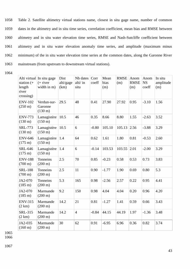
43
Table 2. Satellite altimetry virtual stations name, closest in situ gage name, number of common 1058
dates in the altimetry and in situ time series, correlation coefficient, mean bias and RMSE between 1059
altimetry and in situ water elevation time series, RMSE and Nash-Sutcliffe coefficient between 1060
altimetry and in situ water elevation anomaly time series, and amplitude (maximum minus 1061
minimum) of the in situ water elevation time series at the common dates, along the Garonne River 1062
mainstream (from upstream to downstream virtual stations). 1063
1064
Alti virtual
station (+
length
river
crossing)
In situ gage
(+ river
width in m)
Dist
alti/gage
(km)
Nb dates
alti/ in
situ
Corr
coeff
Mean
bias
(m)
RMSE
(m)
Anom
RMSE
(m)
Anom
NS
coeff
In situ
amplitude
(m)
ENV-102
(250 m)
Verdun-sur-
Garonne
(130 m)
29.5 48 0.41 27.90 27.92 0.95 -3.10 1.56
ENV-773
(130 m)
Lamagistère
(150 m)
10.5 46 0.35 8.66 8.80 1.55 -2.63 3.52
SRL-773
(130 m)
Lamagistère
(150 m)
10.5 6 -0.80 105.10 105.13 2.56 -3.88 3.29
ENV-646
(175 m)
Lamagistère
(150 m)
1.4 64 0.62 1.61 1.80 0.81 -0.53 2.60
SRL-646
(175 m)
Lamagistère
(150 m)
1.4 6 -0.14 103.53 103.55 2.01 -2.00 3.29
ENV-188
(700 m)
Tonneins
(200 m)
2.5 70 0.85 -0.23 0.58 0.53 0.73 3.83
SRL-188
(700 m)
Tonneins
(200 m)
2.5 11 0.90 -1.77 1.90 0.69 0.80 5.3
JA2-070
(185 m)
Tonneins
(200 m)
5.3 165 0.98 -2.56 2.57 0.22 0.95 4.41
JA2-070
(185 m)
Marmande
(200 m)
9.2 150 0.98 4.04 4.04 0.20 0.96 4.20
ENV-315
(2 km)
Marmande
(200 m)
14.2 21 0.81 -1.27 1.41 0.59 0.66 3.43
SRL-315
(2 km)
Marmande
(200 m)
14.2 4 -0.84 44.15 44.19 1.97 -1.36 3.48
JA2-035
(160 m)
Marmande
(200 m)
30 62 0.91 -6.95 6.96 0.36 0.82 3.74
1065
1066
1067
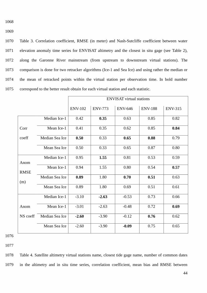
44
1068
1069
Table 3. Correlation coefficient, RMSE (in meter) and Nash-Sutcliffe coefficient between water 1070
elevation anomaly time series for ENVISAT altimetry and the closest in situ gage (see Table 2), 1071
along the Garonne River mainstream (from upstream to downstream virtual stations). The 1072
comparison is done for two retracker algorithms (Ice-1 and Sea Ice) and using rather the median or 1073
the mean of retracked points within the virtual station per observation time. In bold number 1074
correspond to the better result obtain for each virtual station and each statistic. 1075
ENVISAT virtual stations
ENV-102 ENV-773 ENV-646 ENV-188 ENV-315
Corr
coeff
Median Ice-1 0.42 0.35 0.63 0.85 0.82
Mean Ice-1 0.41 0.35 0.62 0.85 0.84
Median Sea Ice 0.50 0.33 0.65 0.88 0.79
Mean Sea Ice 0.50 0.33 0.65 0.87 0.80
Anom
RMSE
(m)
Median Ice-1 0.95 1.55 0.81 0.53 0.59
Mean Ice-1 0.94 1.55 0.80 0.54 0.57
Median Sea Ice 0.89 1.80 0.70 0.51 0.63
Mean Sea Ice 0.89 1.80 0.69 0.51 0.61
Anom
NS coeff
Median Ice-1 -3.10 -2.63 -0.53 0.73 0.66
Mean Ice-1 -3.01 -2.63 -0.48 0.72 0.69
Median Sea Ice -2.60 -3.90 -0.12 0.76 0.62
Mean Sea Ice -2.60 -3.90 -0.09 0.75 0.65
1076
1077
Table 4. Satellite altimetry virtual stations name, closest tide gage name, number of common dates 1078
in the altimetry and in situ time series, correlation coefficient, mean bias and RMSE between 1079
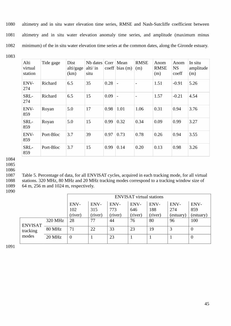
45
altimetry and in situ water elevation time series, RMSE and Nash-Sutcliffe coefficient between 1080
altimetry and in situ water elevation anomaly time series, and amplitude (maximum minus 1081
minimum) of the in situ water elevation time series at the common dates, along the Gironde estuary. 1082
1083
Alti
virtual
station
Tide gage Dist
alti/gage
(km)
Nb dates
alti/ in
situ
Corr
coeff
Mean
bias (m)
RMSE
(m)
Anom
RMSE
(m)
Anom
NS
coeff
In situ
amplitude
(m)
ENV-
274
Richard 6.5 35 0.28 - - 1.51 -0.91 5.26
SRL-
274
Richard 6.5 15 0.09 - - 1.57 -0.21 4.54
ENV-
859
Royan 5.0 17 0.98 1.01 1.06 0.31 0.94 3.76
SRL-
859
Royan 5.0 15 0.99 0.32 0.34 0.09 0.99 3.27
ENV-
859
Port-Bloc 3.7 39 0.97 0.73 0.78 0.26 0.94 3.55
SRL-
859
Port-Bloc 3.7 15 0.99 0.14 0.20 0.13 0.98 3.26
1084
1085
1086
Table 5. Percentage of data, for all ENVISAT cycles, acquired in each tracking mode, for all virtual 1087
stations. 320 MHz, 80 MHz and 20 MHz tracking modes correspond to a tracking window size of 1088
64 m, 256 m and 1024 m, respectively. 1089
1090
ENVISAT virtual stations
ENV-
102
(river)
ENV-
315
(river)
ENV-
773
(river)
ENV-
646
(river)
ENV-
188
(river)
ENV-
274
(estuary)
ENV-
859
(estuary)
ENVISAT
tracking
modes
320 MHz 28 77 44 76 80 96 100
80 MHz 71 22 33 23 19 3 0
20 MHz 0 1 23 1 1 1 0
1091

46
1092
Figures 1093 1094
1095
1096
Figure 1. Garonne basin (white boundaries), with in situ gages (green dots), ENVISAT and SARAL
virtual stations (red dots) and Jason-2 virtual stations (magenta dots) used in this study. Dotted red
lines correspond to ENVISAT and SARAL ground tracks. Magenta lines correspond to Jason-2
ground tracks. Background colors correspond to a MODIS image from 01 October 2011, whose
color has been artificially lightened using a shaded relief, computed from a DEM provided by IGN,
over the Garonne basin. Location of the Garonne basin in France main territory is shown in the
bottom right hand corner map (white boundaries)
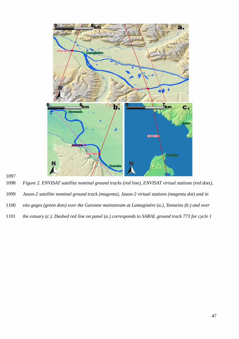
47
1097
Figure 2. ENVISAT satellite nominal ground tracks (red line), ENVISAT virtual stations (red dots), 1098
Jason-2 satellite nominal ground track (magenta), Jason-2 virtual stations (magenta dot) and in 1099
situ gages (green dots) over the Garonne mainstream at Lamagistère (a.), Tonneins (b.) and over 1100
the estuary (c.). Dashed red line on panel (a.) corresponds to SARAL ground track 773 for cycle 1 1101
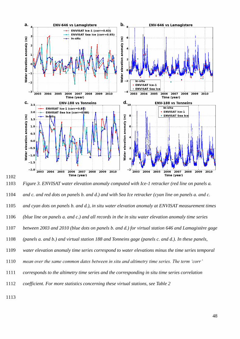
48
1102
Figure 3. ENVISAT water elevation anomaly computed with Ice-1 retracker (red line on panels a. 1103
and c. and red dots on panels b. and d.) and with Sea Ice retracker (cyan line on panels a. and c. 1104
and cyan dots on panels b. and d.), in situ water elevation anomaly at ENVISAT measurement times 1105
(blue line on panels a. and c.) and all records in the in situ water elevation anomaly time series 1106
between 2003 and 2010 (blue dots on panels b. and d.) for virtual station 646 and Lamagistère gage 1107
(panels a. and b.) and virtual station 188 and Tonneins gage (panels c. and d.). In these panels, 1108
water elevation anomaly time series correspond to water elevations minus the time series temporal 1109
mean over the same common dates between in situ and altimetry time series. The term ‘corr’ 1110
corresponds to the altimetry time series and the corresponding in situ time series correlation 1111
coefficient. For more statistics concerning these virtual stations, see Table 2 1112
1113
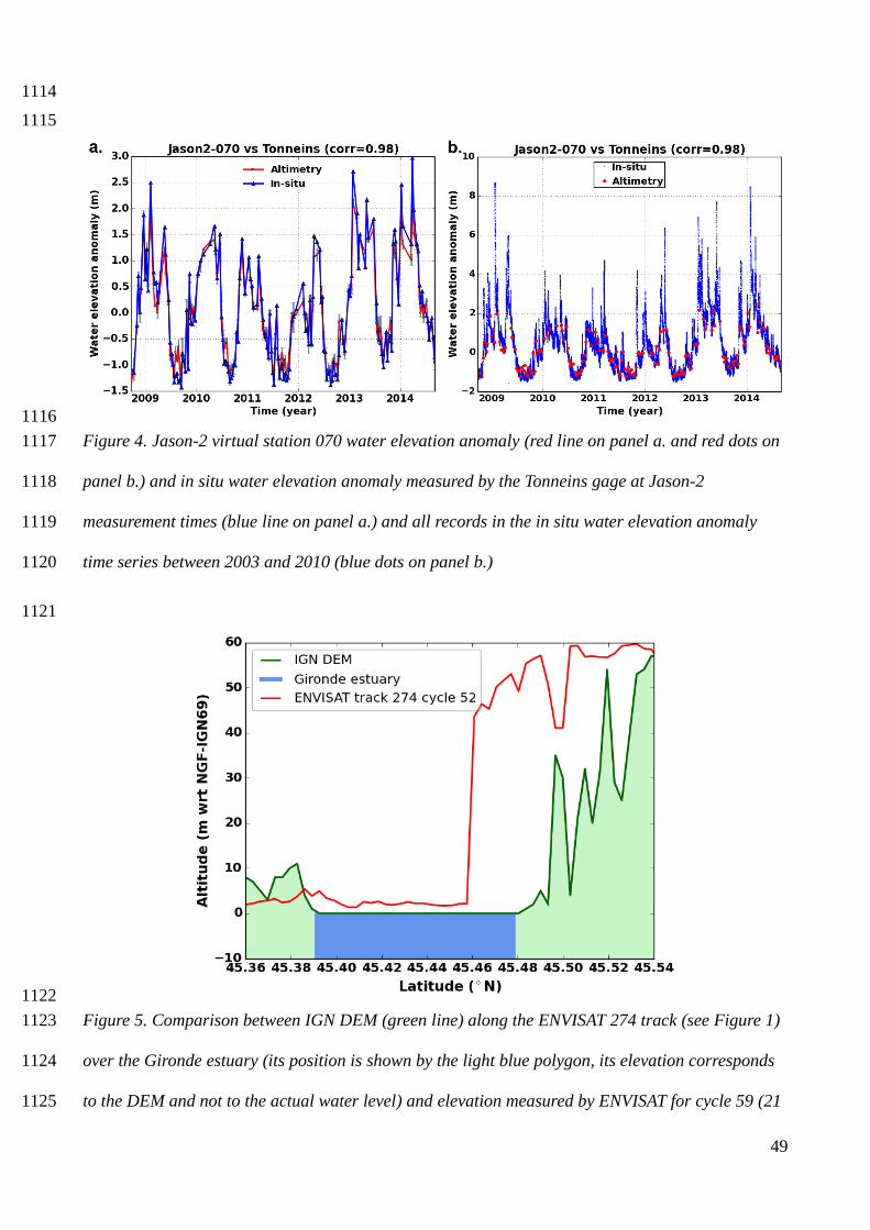
49
1114
1115
1116
Figure 4. Jason-2 virtual station 070 water elevation anomaly (red line on panel a. and red dots on 1117
panel b.) and in situ water elevation anomaly measured by the Tonneins gage at Jason-2 1118
measurement times (blue line on panel a.) and all records in the in situ water elevation anomaly 1119
time series between 2003 and 2010 (blue dots on panel b.) 1120
1121
1122
Figure 5. Comparison between IGN DEM (green line) along the ENVISAT 274 track (see Figure 1) 1123
over the Gironde estuary (its position is shown by the light blue polygon, its elevation corresponds 1124
to the DEM and not to the actual water level) and elevation measured by ENVISAT for cycle 59 (21 1125
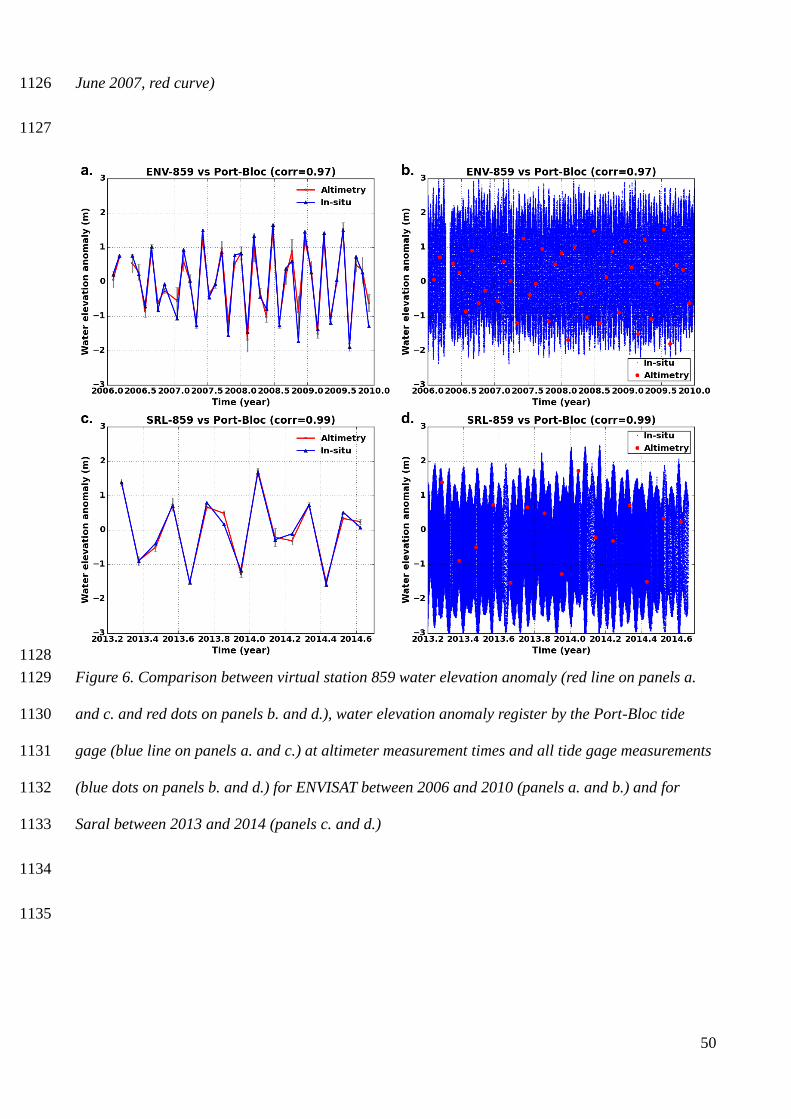
50
June 2007, red curve) 1126
1127
1128
Figure 6. Comparison between virtual station 859 water elevation anomaly (red line on panels a. 1129
and c. and red dots on panels b. and d.), water elevation anomaly register by the Port-Bloc tide 1130
gage (blue line on panels a. and c.) at altimeter measurement times and all tide gage measurements 1131
(blue dots on panels b. and d.) for ENVISAT between 2006 and 2010 (panels a. and b.) and for 1132
Saral between 2013 and 2014 (panels c. and d.) 1133
1134
1135
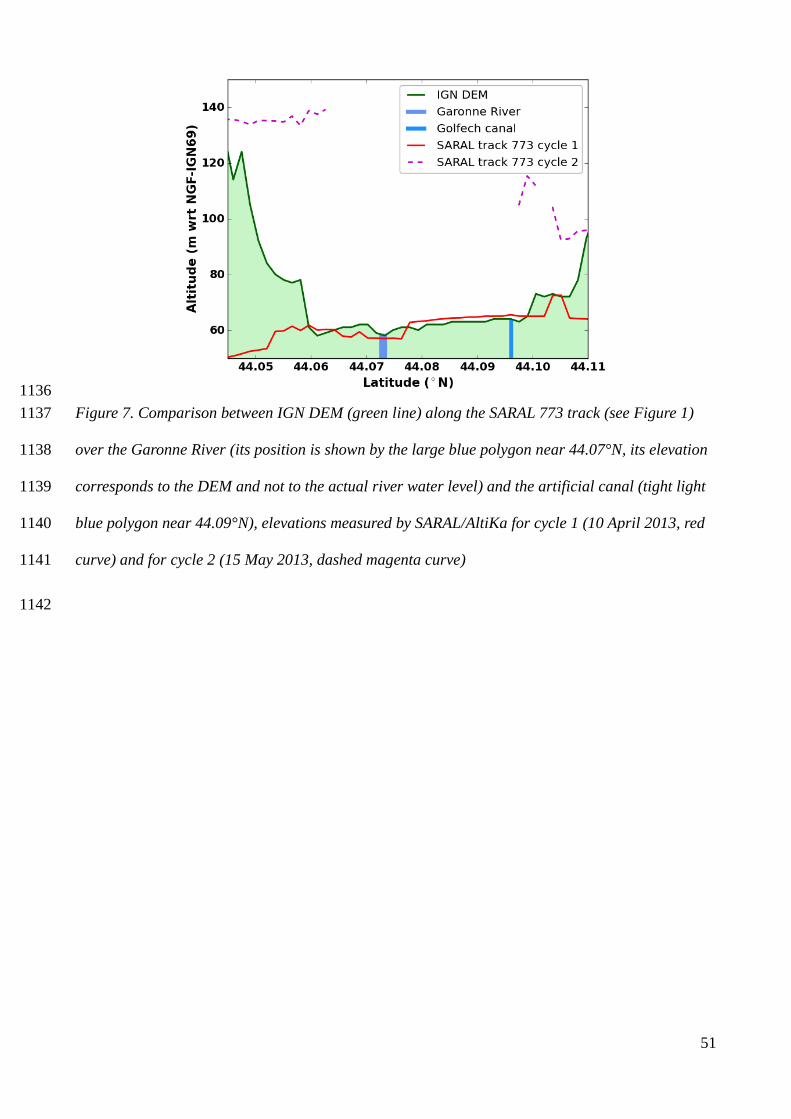
51
1136
Figure 7. Comparison between IGN DEM (green line) along the SARAL 773 track (see Figure 1) 1137
over the Garonne River (its position is shown by the large blue polygon near 44.07°N, its elevation 1138
corresponds to the DEM and not to the actual river water level) and the artificial canal (tight light 1139
blue polygon near 44.09°N), elevations measured by SARAL/AltiKa for cycle 1 (10 April 2013, red 1140
curve) and for cycle 2 (15 May 2013, dashed magenta curve) 1141
1142
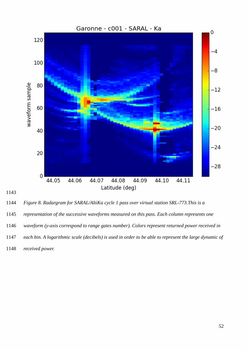
52
1143
Figure 8. Radargram for SARAL/AltiKa cycle 1 pass over virtual station SRL-773.This is a 1144
representation of the successive waveforms measured on this pass. Each column represents one 1145
waveform (y-axis correspond to range gates number). Colors represent returned power received in 1146
each bin. A logarithmic scale (decibels) is used in order to be able to represent the large dynamic of 1147
received power. 1148