satellite-derived tropical cyclone intensity in the...

Satellite-Derived Tropical Cyclone Intensity in the North Pacific Ocean Using theDeviation-Angle Variance Technique

ELIZABETH A. RITCHIE AND KIMBERLY M. WOOD

Department of Atmospheric Sciences, The University of Arizona, Tucson, Arizona

OSCAR G. RODRIGUEZ-HERRERA, MIGUEL F. PINEROS, AND J. SCOTT TYO

College of Optical Sciences, The University of Arizona, Tucson, Arizona

(Manuscript received 7 February 2013, in final form 14 November 2013)

ABSTRACT

The deviation-angle variance technique (DAV-T), whichwas introduced in theNorthAtlantic basin for tropical

cyclone (TC) intensity estimation, is adapted for use in the North Pacific Ocean using the ‘‘best-track center’’

application of the DAV. The adaptations include changes in preprocessing for different data sources [Geosta-

tionary Operational Environmental Satellite-East (GOES-E) in the Atlantic, stitched GOES-E–Geostationary

Operational Environmental Satellite-West (GOES-W) in the eastern North Pacific, and the Multifunctional

Transport Satellite (MTSAT) in the western North Pacific], and retraining the algorithm parameters for

different basins. Over the 2007–11 period, DAV-T intensity estimation in the western North Pacific results in

a root-mean-square intensity error (RMSE, as measured by the maximum sustained surface winds) of 14.3 kt

(1 kt’ 0.51m s21) when compared to the Joint TyphoonWarning Center best track, utilizing all TCs to train

and test the algorithm. The RMSE obtained when testing on an individual year and training with the re-

maining set lies between 12.9 and 15.1 kt. In the eastern North Pacific the DAV-T produces an RMSE of

13.4 kt utilizing all TCs in 2005–11when compared with theNationalHurricaneCenter best track. TheRMSE

for individual years lies between 9.4 and 16.9 kt. The complex environment in the western North Pacific led to

an extension to the DAV-T that includes two different radii of computation, producing a parametric surface

that relates TC axisymmetry to intensity. The overall RMSE is reduced by an average of 1.3 kt in the western

North Pacific and 0.8 kt in the eastern North Pacific. These results for the North Pacific are comparable with

previously reported results using the DAV for the North Atlantic basin.

1. Introduction

a. Intensity estimation from remote sensing data

Unlike land-based surface observations, in situ sur-

face observations over the tropical oceans are sparse.

This lack of data results in a heavy reliance on satellite

observations in order tomonitor severe weather systems

such as tropical cyclones (TCs). Using these satellite

measurements, it is possible to estimate TC intensity

when direct measurements are not available. TheDvorak

technique (Dvorak 1975) and its extended versions, the

objective Dvorak technique (Velden et al. 1998) and the

advanced Dvorak technique (Olander and Velden 2007),

are well-known examples of methodologies to estimate

themaximumsustained surfacewinds of TCs from satellite

imagery. In the original Dvorak technique, the analyst

considers patterns and cloud-top temperatures in a se-

ries of satellite images, classifying the scenes according

to predefined patterns and assigning a T number based

on the features of the classification. The performance of

the technique in the North Atlantic and eastern North

Pacific basins is described in Knaff et al. (2010). Other

procedures are based on the Advanced Microwave

Sounding Unit as described in Demuth et al. (2004) and

Spencer and Braswell (2001). Microwave frequencies

can reveal important structural features that are ob-

scured by high-level cirrus and thus cannot be observed

Corresponding author address: E. A. Ritchie, Dept. of Atmo-

spheric Sciences, The University of Arizona, P.O. Box 210081,

Tucson, AZ 85721-0081.

E-mail: [email protected]

JUNE 2014 R I TCH IE ET AL . 505

DOI: 10.1175/WAF-D-13-00133.1

� 2014 American Meteorological Society

mailto:[email protected]

by infrared imagers. However, limitations exist for each

of these techniques, and, in some cases, their performance

depends on the skill of the user. It should also be noted

that the absence of aircraft reconnaissance in the west-

ern and eastern North Pacific basins makes it difficult to

compare the intensity estimates with in situ observations.

b. The deviation-angle variance technique

The deviation-angle variance technique (DAV-T),

a method that can be used to estimate the intensity of

TCs, was described and applied to the North Atlantic

basin by Pi~neros et al. (2008, 2011) and Ritchie et al.

(2012). Here, intensity is defined as the maximum 1-min

sustained 10-m surface wind speed near the core of the

TC. This technique quantifies the axisymmetry of TCs in

IR satellite imagery by performing a statistical analysis

of the direction of the gradient of the IR brightness

temperatures. The brightness temperature gradient vec-

tors are more aligned along radials of an intense TC than

the vectors computed from a weak, disorganized tropi-

cal system. This degree of storm organization can be

quantified by calculating the variance of the angle be-

tween the gradient vector and the radial at each pixel in

the scene. Previous results for the North Atlantic basin

show that the variance of this deviation angle is nega-

tively correlated with the TC’s intensity (Pi~neros et al.

2008). Although the original application of the tech-

nique was completely objective with an automated center-

finding routine in place, there were significant errors in

the intensity estimation for a very small number of

highly sheared cases of TCs (Pi~neros et al. 2011). An

updated version, which used the National Hurricane

Center’s best-track archive to center the algorithm,

yielded significant improvements in the specific sheared

cases. Root-mean-square (RMS) intensity errors using

the best-track center version of the DAV-T for the

North Atlantic basin over the period 2004–10 were

12.9 kt (1 kt 5 0.51m s21) (Ritchie et al. 2012), an im-

provement of 1.8 kt over the automated center routine.

In this paper, this same DAV-T for intensity estima-

tion is adapted to the eastern and western North Pacific

basins. The best parameters for DAV-T are determined,

and the method is expanded to accommodate the more

diverse storm characteristics that are present in these

basins. In section 2, this methodology is briefly dis-

cussed, and the method for stitching imagery from two

separate geostationary satellites to be used in the east-

ern North Pacific is described. The results found when

applying the technique to the western North Pacific are

described in section 3. Section 4 discusses the perfor-

mance of the DAV-T in the eastern North Pacific. Fi-

nally, section 5 presents some conclusions and details

future development work.

2. Methodology

a. IR imagery used for the DAV-T

This paper presents results from two different intensity

estimation studies: one in the western North Pacific and

one in the eastern North Pacific. The data for the west-

ern North Pacific portion of this study are derived from

longwave (10.7mm) IR satellite imagery from the Japan-

based Multifunctional Transport Satellite (MTSAT)

over the western North Pacific basin. The images used in

the western North Pacific study are resampled to a spa-

tial resolution of 10 kilometers per pixel and encompass

an area from 08 to 408N and from 1008E to 1808.The data for the easternNorthPacific study are derived

from longwave (10.7mm) IR satellite imagery obtained

from the Geostationary Operational Environmental

Satellite-West (GOES-W) and -East (GOES-E). Data are

obtained from both satellites as GOES-W does not cover

the extreme eastern part of the eastern North Pacific

basin. These images are also resampled to a spatial

resolution of 10 kilometers per pixel. To cover the lon-

gitudinal extent of the basin, GOES-W images are

stitched with GOES-E images after resampling in order

to generate the final data used in the study. The re-

sampled image from each satellite is blended using

a column of pixels centered near 104.78W and averaging

the data from each image out to four pixels on either side

of this center pixel in order to account for slight shifts re-

sulting from the 15-min time difference between each

satellite image. The final stitched images encompass an

area from 08 to 408N and from 1708 to 808W.

Similar to previous versions of the technique, those

samples when the TC center is over land (continental

land and large islands) in each basin are removed from

the analysis. This removal does not affect the ability to

use the technique near and over small islands. Further-

more, RMS intensity errors for near-land (0–250 km)

samples are very close to the overall RMS intensity error

for all samples (data not shown).

The western North Pacific study considers images that

include existing TCs from the 2007–11 typhoon seasons

and comprise a total of 22 552 unique hourly images. The

resulting dataset includes 12 supertyphoons, 32 typhoons,

27 tropical storms, and 18 tropical depressions. Fur-

thermore, of the 22 552 images, 47% are tropical de-

pression intensity, 27%are tropical storm intensity, 24%

are typhoon intensity, and 2% are supertyphoon inten-

sity. The eastern North Pacific study examines images

with existing TCs from the 2005–11 hurricane seasons

and comprises a total of 20 213 unique half-hourly im-

ages. The resulting dataset includes 21 major hurricanes,

25 hurricanes, and 44 tropical storms. The North At-

lantic hurricane database (HURDAT) does not include

506 WEATHER AND FORECAST ING VOLUME 29

systems that peaked below tropical storm (34 kt) in-

tensity; thus, none of these cases was included in the

analysis.Of the 20213 images, 38%are tropical depression

intensity, 40% are tropical storm intensity, 15% are hur-

ricane intensity, and 7% are major hurricane intensity.

Examples of the IR image data analyzed in this study

are shown in Fig. 1. The western North Pacific image

(Fig. 1a) contains Typhoons Parma and Melor (2009),

and the eastern North Pacific image (Fig. 1b) includes

Hurricanes Celia and Darby (2010). The results of ap-

plying theDAV-T to these data are compared against the

best-track databases from the Joint Typhoon Warning

Center (JTWC; http://www.usno.navy.mil/NOOC/nmfc-

ph/RSS/jtwc/best_tracks/) and the National Hurricane

Center (NHC; http://www.nhc.noaa.gov/data/#hurdat).

b. Tropical cyclone intensity estimation

The DAV-T was introduced in Pi~neros et al. (2008) as

a procedure to objectively estimate the intensity of TCs.

The procedure quantifies the level of axisymmetry of TC

brightness temperatures by computing the gradient of

the brightness temperatures from the infrared images

and then calculating the deviation angle of the gradient

vectors with respect to a radial projected from a defined

center. The amount of deviation from the perfect radial

indicates the level of alignment of the gradient vectors.

An example of this calculation for a single gradient vector,

when the center is located in the eye of the vortex, is

shown in Fig. 2a. The variance of the distribution of angles

within a defined radius from the center then quantifies the

axisymmetry of the cyclone relative to that center point

(Fig. 2b). The DAV decreases at a given center point as

the system becomes more axisymmetric about that point,

since the gradient vectors within the calculation radius are

pointing more uniformly toward or away from the center.

In contrast, the DAV increases when the orientation of

the gradient vectors becomes increasingly asymmetric with

respect to that center point. This asymmetry is characteristic

FIG. 1. (a)MTSAT IR image of thewesternNorth Pacific at 1230UTC 4Oct 2009. The image

includes Typhoon Melor (72m s21, 911 hPa) near 1408E and Typhoon Parma (60m s21,

978 hPa) near 1208E, surrounded by nondeveloping cloud clusters. (b) Stitched GOES-W–

GOES-E IR image at 0000 UTC 25 Jun 2010. The image includes Hurricane Celia (72m s21,

921 hPa) near 1158W and Hurricane Darby (41m s21, 977 hPa) near 1008W.


http://www.usno.navy.mil/NOOC/nmfc-ph/RSS/jtwc/best_tracks/

http://www.usno.navy.mil/NOOC/nmfc-ph/RSS/jtwc/best_tracks/

http://www.nhc.noaa.gov/data/#hurdat

of nondeveloping cloud clusters, sheared TCs, and other

disorganized cloud structures. Whereas the fully auto-

mated system used the minimum variance point to per-

form the intensity estimation (Pi~neros et al. 2011),

Ritchie et al. (2012) updated the intensity estimation

algorithm by using a known center pixel as a reference

for the calculation. The system can now be operated

using automatic centers, best-track centers, or any other

center point defined by the user. Recent results in the

North Atlantic basin showed that the use of best-track

TC fixes provided measurable improvements in the inten-

sity estimate over the original automated center-finding

methodology (Ritchie et al. 2012). Therefore, in this

study the best-track positions are used in both basins to

constrain the intensity estimation.

For intensity estimation, the DAV values are obtained

at the single pixel location identified in the best-track

archives of the operational centers. For the western North

Pacific study, MTSAT IR images are available hourly,

and thus the 6-h best-track positions are interpolated

using a cubic spline interpolation to match the times of

the IR images. For the eastern North Pacific study, GOES

images are available half-hourly, and the 6-h best-track

positions are again interpolated to match the temporal

resolution of the IR imagery. The western North Pacific

(eastern North Pacific) best-track intensity values are

linearly interpolated to hourly (half hourly) resolution

to properly compare these data with theDAVestimates.

The DAV-T has been well tested in the North At-

lantic, leading to annual RMS intensity errors of 10–14 kt

(Ritchie et al. 2012). In the majority of the years in

the North Atlantic, the performance of the DAV-T is

optimized at a radius of calculation of 200–250 km.

However, because there are differences in both the

large-scale environment and the modes of genesis be-

tween the North Atlantic and western North Pacific

basins (e.g., Lander 1994; Ritchie and Holland 1999;

Briegel and Frank 1997; Ritchie et al. 2003), with con-

siderably more variety in the sizes and structures of TCs

in the western North Pacific (e.g., Lander 1994), it is

expected that the DAV-T parameters would be different

for the North Pacific from those chosen for the North

Atlantic. Therefore, the DAV-T is tested over eight dif-

ferent radii of DAV calculation, varying from 150 to

500 km in steps of 50 km, in order to capture the large size

variability of the TCs in the North Pacific.

Similar to the North Atlantic technique, the DAV

time series is smoothed in both basins using a low-pass

filter (impulse response of e-t/t) with a filter time con-

stant of 100 h. The filtering reduces high-frequency os-

cillations in the DAV time series allowing for better

comparison with the highly smoothed interpolated best-

track intensity estimates. However, the filter also in-

troduces a time delay that can lead to errors in rapidly

intensifying cases (Ritchie et al. 2012).

After computing the DAV values, the western and

eastern North Pacific datasets are divided into two sub-

sets: a training set comprising all samples from all but

one of the years, and an independent testing set com-

prising all samples from the excluded year. The training

set is used to calculate a parametric curve that relates the

TC intensity with theDAV signal for each basin, and the

testing set is used to independently test the accuracy of

the wind speed estimate produced by this parametric

curve. A sigmoid curve unique to each basin is fitted to

the training data. The curve for the western North Pa-

cific is given by

f (s2)5140

11 exp[a(s21b)]1 25 kt , (1)

and the curve for the eastern North Pacific is given by

FIG. 2. (a) Deviation-angle calculation for a gradient vector, where the center is located in the eye of the tropical cyclone.

(b) Distribution of angles for the calculation using the center (eye) pixel. The variance of the histogram is (12168)2. (c) Map of

variances (8)2 calculated by performing the DAV calculation using each pixel in turn as the center pixel and mapping the variance

value back to that pixel.


f (s2)5130

11 exp[a(s21b)]1 25 kt, (2)

where s2 is the DAV value and a and b are two free

parameters that describe the relation between the axi-

symmetry parameter and the best-track intensity esti-

mates. The parameters a and b fromEqs. (1) and (2) are

fit to minimize the mean square error from the in-

terpolated best-track data. Note that Eq. (1) constrains

the minimum intensity that can be estimated in the west-

ern North Pacific to 25 kt and the maximum intensity to

165 kt, and Eq. (2) restricts the eastern North Pacific to

a range of 25–155 kt.

Examples of the two-dimensional histogram of the

filtered DAV samples and the best-track intensity for

both basins are provided in Fig. 3. The western North

Pacific training set is composed of all 89 TCs during the

period 2007–11 shown for a radius of 300 km (Fig. 3a),

and the eastern North Pacific training set is composed of

all 90 TCs during the period 2005–11 shown for a radius

of 200 km (Fig. 3b). Finally, the RMS intensity errors for

both basins are calculated by comparing the DAV-T-

derived intensity estimates to the best-track archived

intensity estimates from the JTWC (western North Pa-

cific) and the NHC (eastern North Pacific).

3. Results for the western North Pacific basin

a. Tropical cyclone intensity estimation

Testing for the intensity estimation was accomplished

in twoways. First, an overall test result was calculated by

training on all five years of data and then testing on those

same five years for all eight radii (150–500 km) of the

DAV calculation. A second result was obtained by with-

holding each year, training on the other four years to

create the DAV parametric curve, and using the re-

sulting curve to estimate wind speed intensities for the

withheld year. The DAV intensity estimates were then

compared with the interpolated JTWC best-track in-

tensity records by calculating the RMS intensity error

between the two intensity signals. The result of training

on 2007–10 and testing on 2011 is shown in Fig. 4a as an

example. Average RMS intensity errors for the test on

all five of the years and for each test year using several

different radii of DAV calculation are shown in Table 1.

As given in Table 1, training on all 89 storms and then

testing on those same 89 storms produces a best overall

RMS intensity error of 14.3 kt using a radius of calcu-

lation of 300 km. Furthermore, RMS intensity errors

vary between 12.9 and 15.1 kt for the individual years

(Table 1, Fig. 4a). These results are not particularly

sensitive to small changes in the sigmoid parameters. In

addition, the technique performs best for a calculation

radius of 300 km, and this is consistent through the years

of the study. This suggests that the axisymmetric struc-

ture of the clouds within about 300 km of the center as

measured by the DAV technique generally has the high-

est correlation with the intensity of the TC in the western

North Pacific basin.

Further analysis shows that western North Pacific TCs

tend to partition into two groups of storms: those that

are best characterized by a radius of calculation of 200–

300 km, and those large storms that are better charac-

terized by a radius of calculation of 450–500 km (e.g.,

Fig. 5b). We suspect that this is a result of the more

complex mechanisms that modulate TC size and structure

in the monsoon environment of the western North

FIG. 3. (a) A 2D histogram of the 300-km-filtered DAV samples

and best-track intensity estimates using (208)2 3 5 kt bins for 89

western North Pacific tropical cyclones from 2007 through 2011.

(b) A 2D histogram of the 200-km-filtered DAV samples and best-

track intensity estimates using (208)23 5 kt bins for 90 eastern North

Pacific tropical cyclones from 2005 through 2011. In each panel the

black line corresponds to the best-fit sigmoid curve for themedian of

the samples.


Pacific compared to those in the North Atlantic (e.g.,

Chang and Song 2006; Harr et al. 1996a,b). This vari-

ability results in TCs that range in size from ‘‘midgets,’’

with radii less than 200 km [e.g., Typhoon Ellie 1991; see

Lander (1994) and Joint Typhoon Warning Center

(1991)], to ‘‘giants,’’ with radii greater than 1000 km

[e.g., Supertyphoon Tip 1979; see Joint Typhoon

Warning Center (1979)]. In many cases, the core of the

TC may be surrounded by disorganized cloud clusters

associated with the monsoon trough. These cloud clus-

ters are not directly associated with the TC, but they

adversely impact the technique when they are included

in the DAV calculation. In these cases, a small radius of

DAV calculation is desirable. Alternatively, for those

larger TCs that form in the monsoon trough with asso-

ciated banding structures, a larger radius of DAV

FIG. 4. (a)WesternNorthPacific intensity estimates andbest-track intensities for 2011by training on 2007–10 to calculate

theDAV-T–intensity parametric curve. TheRMS intensity error is 12.9kt. (b)EasternNorth Pacific intensity estimates and

best-track intensities for 2008 by training on 2005–07 and 2009–11 to calculate the DAV-T–intensity parametric curve. The

RMS intensity error is 10.0kt. Individual TCs are identified under each panel.

TABLE 1. RMS intensity error (kt) for every radius of DAV calculation (150–450km), number of storms, and number of samples for each

individual year for the western North Pacific. The lowest annual RMS intensity errors are highlighted in italics.

Year 150 km 200 km 250km 300 km 350 km 400 km 450 km TCs No. of samples

2007 19.4 17.0 14.5 13.7 14.3 14.7 15.2 23 6368

2008 18.1 17.1 15.8 15.1 15.4 15.7 16.2 14 3821

2009 17.5 15.9 15.1 16.0 16.8 16.9 17.1 15 5042

2010 18.7 16.5 14.9 14.0 14.1 14.6 14.9 19 4915

2011 18.6 15.8 14.2 12.9 14.1 14.9 16.0 18 2406

All 18.5 16.5 14.9 14.3 14.8 15.3 15.7 89 22 552


calculation is more appropriate. Figure 5 shows an ex-

ample of those features that introduce noise to theDAV

calculation for small TCs embedded within monsoon

cloudiness but are desirable for large TCs. In Fig. 5a the

circular core of Supertyphoon Sepat is detached from

the cloudiness to the south by a narrow dark moat re-

gion, which is associatedwithmonsoonal southwesterlies.

The size of Sepat, as measured by the radius of 34-kt

winds at this time, is approximately 200km according to

the JTWC best-track archive, and the entire system is

enclosed by the dashed black circle (250-km radius). In

contrast, in Fig. 5b it is more difficult to distinguish the

surrounding clouds from the inner core of TyphoonMan-

Yi.At this time, the JTWCbest-track archive lists the size

of the storm as approximately 270 km.Here, the rainband

features are inseparable from the core and appear to be

an integral part of the TC structure. This analysis will be

expounded upon further in section 3b.

Finally, categorizing by intensity bins (Table 2) results

in a similar trend as is found in the North Atlantic

(Ritchie et al. 2012). For the highest intensities (above

64 kt), the combined RMS intensity error is 19.5 kt, and

more storms are underestimated than overestimated.

For tropical storms, the RMS intensity error is 13.8 kt,

and the majority of samples are again underestimated.

The RMS intensity error for tropical depression in-

tensities is 11.0 kt. This sample constitutes 47% of the

population, and 82%of these samples are overestimated

by the technique. As discussed inRitchie et al. (2012) for

the North Atlantic basin, these biases are at least partly

due to the choice of the parametric curve used to fit the

training data (e.g., Fig. 3a). The curve tends to under-

estimate the higher-intensity values and overestimate

the lower-intensity values (Table 2). A lack of training

data at the highest end of the intensity spectrum com-

pounds the problem. We are currently working on other

parametric methods to address this problem.

b. Tropical cyclone size variability and thetwo-dimensional training surface

Asmentioned in the previous section, the large variety

of TC sizes and structures that exists in the predominantly

monsoon trough environment of the western North Pa-

cific presents a challenge for a scheme that measures the

structure of the clouds. One solution is to find a way to

automatically take the size of the storm into account,

either as an average over its life or at any instant in time.

However, this is extremely challenging as there are no

FIG. 5. (a) Supertyphoon Sepat (110 kt, 941 hPa) at 1630 UTC 14 Aug 2007. (b) Typhoon

Man-Yi (100kt, 948hPa) at 1130UTC11 Jul 2007. In both images, the circles indicate the 250-km

(dashed) and 450-km (solid) radii, respectively.

TABLE 2. The number of samples, RMSE (kt), and the number of samples either overestimated or underestimated for all of the western

North Pacific samples categorized into bins based on the JTWC’s scale of tropical cyclone intensities.

Bin No. of samples RMSE (kt) No. overestimated No. underestimated

Tropical depression (,34 kt) 10 621 11.0 8693 (82%) 1928 (18%)

Tropical storm (34–63kt) 6197 13.8 2065 (33%) 4132 (67%)

Typhoon (64–129kt) 5324 19.5 1755 (33%) 3569 (67%)

Supertyphoons (.129 kt) 410 19.5 46 (11%) 364 (89%)


reliable, continuous measurements of the storm size

currently available. We are studying methods that allow

the optimum calculation radius to be objectively esti-

mated from the brightness temperature data directly,

but to date have not found a robust solution.

Figure 5 shows two examples of storms from 2007

(best overall performance radius of 300 km) that were

best characterized by the DAV calculated over very

different radii. Supertyphoon Sepat (Fig. 5a) was a small-

to medium-sized TC characterized by a circular core of

cold brightness temperatures, separated from but em-

bedded in monsoonal southwesterlies, and it is best

represented by a radius of 250 km. Using this small ra-

dius to train and test theDAVresults in anRMS intensity

error over the storm’s lifetime of 13.3 kt, in comparison to

the RMS intensity error of 18 kt found from the overall

best 300-km radius of calculation. Typhoon Man-Yi

(Fig. 5b) was a medium- to large-sized TC character-

ized by spiral bands extending more than 500 km from

the center of the storm. The best performance from the

DAV is achieved by using a radius of calculation of

400 km, which produced a lifetime RMS intensity error

of 14.9 kt in comparison with 16 kt found from a 300-km

radius of calculation. Note that, for Supertyphoon Sepat,

a large radius of 400 km yields an RMS intensity error of

32.3 kt, while a small radius of 250 km yields an RMS

intensity error of 17.2 kt for the larger TyphoonMan-Yi.

It appears that the size of the individual storm may have

a bearing on the best radius over which the DAV anal-

ysis should be performed. It is even plausible that, as

storms change size during their lifetime, a suitably varying

radius of calculationmay produce themost accurateDAV

intensity estimates. This is an ongoing subject of research.

Sifting through the entire dataset reveals that the

western North Pacific TCs tend to fall into one of three

categories: 1) those that are small and surrounded by

peripheral monsoon cloudiness and only perform well

with a radius of DAV calculation of 200–250 km, 2) those

that are large and only perform well with a radius of

DAV calculation of 400–500 km, and 3) those systems

that show no preference for a small or large radius of

DAV calculation. To accommodate the first two classes

of tropical cyclones, a set of DAV training data is speci-

fied using a combination of two radii calculations: a small

radius and a large radius. A rectangular grid surrounding

the entire set of training data is defined as an array of

nodes to describe a two-dimensional fitted surface. The

fittingmethodworks by expressing the value of the surface

at points within the rectangular grid as a regularized linear

regression problem, where the regularization is used to

assure the existence of the solution when the number of

grid points (i.e., the number of nodes) is larger than the

number of sampling points. To build the original problem

matrix, the surface value at the sampling points within

the grid is expressed as a linear combination of the

values that the fitted surface would have at the nodes

surrounding the points. The linear combination is then

written as a matrix, A, given by a relation of the form

Ax5 y , (3)

where x is a vector with the value of the surface at the

nodes and y is a vector with the value of the surface at

the sampling points. The regularizationmatrix is obtained

by forcing the first partial derivatives of the surface in

neighboring regions to be equal at the nodes. This con-

dition may be written as

Bx5 0, (4)

where B is the regularization matrix. The two matrices

are then coupled and the resulting system of linear

equations is solved to find the surface value at the nodes

by finding the vector x that minimizes the coupled sys-

tem of linear equations (D’Errico 2013). Mathemati-

cally, this may be expressed as

(Ax2 y)21 lBx2 , (5)

where l is a parameter that can be used to control the

smoothness of the fitted surface. The resulting two-

dimensional parametric surface is shown in Fig. 6 for

a training set comprising all years and calculated using

the DAV radii of calculation of 250 and 500 km.

For testing purposes, all possible combinations of ra-

dii are tested to find the best performance. Table 3 shows

the best-performing radii when training and testing on

all 89 storms as well as when performing independent

testing on each year. Overall, the RMS intensity error

improves from 14.3 kt with a training radius of 300 km to

13.0 kt with a combination of 250- and 500-km training

radii, and a combination could be found that improves

every individual year’s performance except for 2011.

However, no single combination proves to be best for all

years and only a slight worsening of the RMS intensity

error (by 0.1–0.2 kt) typically occurs when one of the two

radii of calculation contributing to the 2D parametric

surface is changed by a 50-km increment. Significance

testing using a Student’s t test suggests that the results

using only a slightly different parametric surface is typ-

ically not significantly different at the 90% confidence

level.However, when the radii of calculation contributing

to the parametric surface aremore than 150 kmdifferent

in one direction or 100 km in both directions, then the

differences are statistically significant. This suggests that

the results are robust, and small changes in the chosen


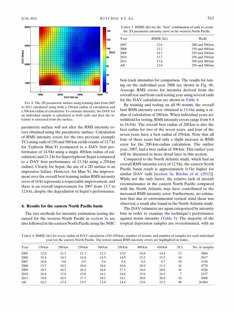
parametric surface will not alter the RMS intensity er-

rors obtained using the parametric surface. Calculation

of RMS intensity errors for the two previous example

TCs using radii of 250 and 500 km yields results of 12.7 kt

for Typhoon Man-Yi (compared to a DAV best per-

formance of 14.9 kt using a single 400 km radius of cal-

culation) and 21.2 kt for Supertyphoon Sepat (compared

to a DAV best performance of 13.3 kt using a 250 km

radius). Clearly for Sepat, the use of a 2D surface is an

impressive failure. However, for Man-Yi, the improve-

ment over the overall best training radius RMS intensity

error of 16 kt represents a respectable improvement, and

there is an overall improvement for 2007 from 13.7 to

12.6 kt, despite the degradation in Sepat’s performance.

4. Results for the eastern North Pacific basin

The two methods for intensity estimation testing dis-

cussed for the western North Pacific in section 3a are

also followed in the easternNorth Pacific using theNHC

best-track intensities for comparison. The results for test-

ing on the individual year 2008 are shown in Fig. 4b.

Average RMS errors for intensity derived from the

overall test and from each testing year using several radii

for the DAV calculation are shown in Table 4.

By training and testing on all 90 storms, the overall

best RMS intensity error obtained is 13.4 kt using a ra-

dius of calculation of 200 km. When individual years are

withheld for testing, RMS intensity errors range from 9.4

to 16.9 kt. The overall best radius of 200 km is also the

best radius for two of the seven years, and four of the

seven years have a best radius of 250 km. Note that all

four of these years had only a slight increase in RMS

error for the 200-km-radius calculation. The outlier

year, 2007, had a best radius of 300 km. This outlier year

will be discussed in more detail later in this section.

Compared to the North Atlantic study, which had an

overall RMS intensity error of 12.9 kt, the eastern North

Pacific basin result is approximately 0.5 kt higher for

similar DAV radii [section 3a; Ritchie et al. (2012)].

While not the only factor, the relative lack of aircraft

reconnaissance in the eastern North Pacific compared

with the North Atlantic may have contributed to the

increased RMS intensity error. Furthermore, no estima-

tion bias due to environmental vertical wind shear was

observed, a result also found in the North Atlantic study.

TheDAVestimates are again categorized by intensity

bins in order to examine the technique’s performance

against storm intensity (Table 5). The majority of the

tropical depression samples are overestimated, with an

FIG. 6. The 2D parametric surface using training data from 2007

to 2011 calculated using both a 250-km radius of calculation and

a 500-km radius of calculation. To estimate intensity, the DAV for

an individual sample is calculated at both radii and then the in-

tensity is extracted from the surface.

TABLE 3. RMSE (kt) for the ‘‘best’’ combination of radii to create

the 2D parametric intensity curve in the western North Pacific.

Year RMSE (kt) Radii

2007 12.6 200 and 500 km

2008 13.3 150 and 400 km

2009 14.7 250 and 500 km

2010 13.7 250 and 350 km

2011 13.0 300 and 400 km

All 13.0 250 and 500 km

TABLE 4. RMSE (kt) for every radius of DAV calculation (150–450km), number of storms, and number of samples for each individual

year for the eastern North Pacific. The lowest annual RMS intensity errors are highlighted in italics.

Year 150 km 200 km 250 km 300 km 350km 400km 450 km TCs No. of samples

2005 12.8 11.3 11.3 12.3 13.0 14.8 14.4 13 3868

2006 19.4 14.3 14.4 14.5 14.9 15.2 15.5 18 5017

2007 10.8 9.6 9.5 9.4 9.4 9.5 9.7 10 3138

2008 13.7 10.2 10.0 10.4 10.6 10.9 11.5 16 4778

2009 18.5 16.5 16.4 16.6 17.5 18.0 18.6 16 4320

2010 16.4 13.8 13.8 14.1 14.8 15.6 16.3 7 2157

2011 19.0 16.9 17.7 18.2 19.1 20.0 20.8 10 3606

All 16.2 13.4 13.5 13.8 14.4 15.0 15.5 90 26 884


RMS intensity error of 10.0 kt. Recall that the parametric

curve for DAV intensity estimation is constrained to

25kt, which is partially responsible for this overestimation.

The tropical storm bin has an RMS intensity error of

11.5 kt, and fewer than half (39%) of the samples are

overestimated. The proportion of underestimated sam-

ples continues to increase for category 1–2 (16.6 kt) and

major hurricane (26.1 kt) samples. Again, the parametric

curve continues to underestimate higher intensity and

overestimate lower-intensity values. The lack of major

hurricane samples also contributes to this under-

estimation issue.Asmentioned earlier, 2007 has the largest

best radius for calculation, 300 km, and also has the

lowest RMS intensity error of 9.4 kt. This year has no

samples above category 1 intensity, which contributes to

its low error value.

As a result of the error improvements in intensity

estimates provided by the two-dimensional surface tech-

nique when used in the western North Pacific (section 3b),

as well as the greater radius and lowRMS intensity error

found when testing 2007, this method is also applied to

the easternNorth Pacific. Again, all combinations of radii

are tested on each individual year as well as on all years.

Table 6 gives the results for the best combination for

each year and for all years. The overall RMS intensity

error improves from 13.4 kt for a radius of 200 km to

12.7 kt for a combination of 200- and 500-km radii. The

individual year RMS intensity errors improve for all

years except 2005 and 2006. The RMS intensity error for

each of the remaining two years increases by 0.2 kt or

less. As with the western North Pacific, no single com-

bination is best for all seven years. It is perhaps not

surprising that the two-radii surface had less impact in

the eastern North Pacific since the size variation of TCs

in this basin is lower and the close proximity of cloudi-

ness not directly associated with the TC is less of a factor

compared with the western North Pacific.

5. Summary and conclusions

In this paper, an objective technique called the

deviation-angle variance technique (DAV-T), which

was developed for the North Atlantic basin to estimate

intensity of TCs from infrared imagery, is applied to the

eastern and western North Pacific basins. We note that

this application of the DAV-T represents a best case

scenario for the technique. The main difference in the

technique as applied to the western North Pacific is the

use of MTSAT data instead of the GOES-E imagery

that is used in the Atlantic basin. Also, instead of solely

using GOES-E imagery in the eastern North Pacific,

stitched GOES-W–GOES-E imagery is employed. Fur-

thermore, the DAV technique is applied to a slightly

larger region, encompassing 08–408N and 1008E–1808 inthe western North Pacific and 08–408N and 1708–808W in

the eastern North Pacific. Finally, the parametric train-

ing curve used in the previous studies to estimate inten-

sity is extended to a two-dimensional parametric surface

in order to better accommodate the larger size and struc-

ture range of TCs in the western North Pacific. This sur-

face is also applied to the eastern North Pacific, though

the resultant error reduction is much more modest in

this basin. TC intensity estimation statistics are calcu-

lated for the years 2007–11 in the western North Pacific

and 2005–11 in the eastern North Pacific. A comparison

with statistics in the North Atlantic basin is included.

In the western North Pacific, the DAV-T shows sim-

ilar results in estimating the intensity of TCs as those

described in Ritchie et al. (2012) for the North Atlantic

basin. A parametric sigmoid-based curve that describes

the relationship between the DAV calculated from the

MTSAT image and the current intensity of the TC is

obtained by fitting to training data calculated from

MTSAT IR images for 89 TCs from 2007 to 2011. The

TABLE 5. The number of samples, RMSE (kt), and the number of samples either overestimated or underestimated for all eastern North

Pacific samples categorized into bins based on the NHC’s scale of tropical cyclone intensities.

Bin No. of samples RMSE (kt) No. overestimated No. underestimated

Tropical depression (,34 kt) 10 254 10.0 8796 (86%) 1458 (14%)

Tropical storm (34–63 kt) 10 759 11.5 4198 (39%) 6561 (61%)

Categories 1 and 2 (64–95kt) 4122 16.6 1405 (34%) 2717 (66%)

Categories 3–5 (.95 kt) 1912 26.1 213 (11%) 1699 (89%)

TABLE 6. RMSE (kt) for the best combination of radii to create the

2D parametric intensity curve in the eastern North Pacific.

Year RMSE (kt) Radii

2005 11.4 200 and 500km

2006 14.5 200 and 300km

2007 8.7 200 and 500km

2008 9.9 250 and 500km

2009 15.4 250 and 500km

2010 13.6 200 and 250km

2011 15.9 150 and 300km

All 12.7 200 and 500km


technique is tested by 1) estimating the intensity of those

same 89 TC cases, and 2) training on four of the five

years and testing on the fifth independent year. The

results are compared with JTWC best-track intensity

estimates by calculating the RMS intensity error over

the entire testing dataset. The minimum RMS intensity

error found was 12.9 kt in 2011, and the overall RMS

intensity error for the 5-yr period was 14.3 kt, which was

approximately 1.4 kt higher than that found in the

North Atlantic. In addition, the DAV parameter was

calculated over several different radii, and it was found

that, in general, a slightly larger radius performed best

in the western North Pacific compared with the North

Atlantic.

Using stitched GOES-W and GOES-E IR imagery to

calculate the brightness temperature gradient and thus

compute theDAV values for each system, theDAV-T is

also tested in the eastern North Pacific. An RMS in-

tensity error of 13.4 kt was calculated using the entire 90-

TC dataset when compared with the NHC best-track

intensity estimates. The minimum error for an indi-

vidual year was 9.4 kt for 2007. Furthermore, a slightly

smaller radius of calculation, 200–250 km, than the

western North Pacific was found to produce the best

errors in the eastern North Pacific.

Similar to the North Atlantic, there is a bias in the

RMS intensity errors for both Pacific basins with lower

errors for weaker storms and higher errors for the more

intense TCs. Much of this bias is attributed to the fitting

of the sigmoid curve, and we are exploring other meth-

odologies to better fit the training data in all basins.

In the monsoonal environment of the western North

Pacific basin, disorganized cloud features typically sur-

round TCs. For those larger TCs, the surrounding mon-

soonal cloudiness is not a factor. However, for those

smaller TCs embedded within the monsoon trough, the

surrounding cloud features introduce noise into the

DAV calculation. Therefore, it is not only the diurnal

and semidiurnal oscillations (Pi~neros et al. 2011), but

also those disorganized portions of the monsoonal clouds

outside the TC, which increase the spread of the DAV-

estimated intensity samples for the western North Pa-

cific. Ultimately, it was determined that the TCs in the

westernNorth Pacific are best described by two different

radii of calculation: one for a smaller area for those TCs

that were smaller in size but embedded in monsoonal

cloudiness that tended to muddy the calculation, and

one for a larger area for those average- to large-sized

TCs to appropriately capture their rainband structure.

To accommodate this dual nature, a two-dimensional

parametric surface was fitted to training data that have

been calculated using two different radii. Error statistics

were compiled using all combinations of DAV radii and,

overall, RMS intensity errors were decreased by 1.3 kt

using the two-dimensional parametric curve (Table 3).

This same methodology was applied to the eastern North

Pacific 7-yr dataset, which decreased the overall RMS

intensity error by 0.7 kt (Table 6).

Future work includes exploring the use of the two-

dimensional parametric curve for the North Atlantic

basin. In addition, the added benefit of including a

variable-size DAV calculation for intensity, particularly

for the western North Pacific, is being explored. While it

is currently difficult to obtain reasonable size estimates

of TCs from observations, we have been exploring this

capability through both the use of simulatedTCdata (K. E.

Ryan et al. 2013, unpublished manuscript), and also by

developing size parameters based on the IR imagery. In

addition, a key component of an intensity estimation

technique is to be able to test it in an operational setting

over several years in order to collect robust statistics of

its performance under these conditions. To achieve this

goal, there are several small steps that need to be ac-

complished: the 6-hourly best-track center needs to be

replaced by an hourly or half-hourly real-time fix, the

first 24 h of the filter for the DAV signal needs to be

calculated differently, and finally we have to determine

the most effective way to report the estimated intensity

from the DAV technique since the half-hourly DAV-

based value oscillates compared to the smooth 3- or 6-h

operational estimates. Finally, because there is no air-

craft reconnaissance program in the western North Pa-

cific, the JTWC best-track archive is heavily reliant on

Dvorak estimates of intensity. Similarly, infrequent air-

craft reconnaissance in the eastern North Pacific also

increases the reliance on Dvorak intensity estimates in

this basin. Our intention is to explore methods of vali-

dating our results using periods when the best-track ar-

chives were enhanced by other observations of intensity,

including those times when scatterometer data and data

from special field campaigns such as the Tropical Cy-

clone Structure-2008 (TCS-08) and Impacts of Ty-

phoons on the Ocean in the Pacific (ITOP) programs

were available.

Acknowledgments. TC best-track data were obtained

from the Joint Typhoon Warning Center (http://www.

usno.navy.mil/NOOC/nmfc-ph/RSS/jtwc/) and the Na-

tional Hurricane Center (http://www.nhc.noaa.gov/data/

#hurdat). This study has been supported by the NOPP

program under Office of Naval ResearchGrant N00014-

10-1-0146. Many thanks to Mr. Jeff Hawkins, Mr. Rich

Bankert, and Mr. Kim Richardson from the Naval Re-

search Laboratory, Monterey, California, who provided

preprocessed MTSAT infrared imagery for this study.

We would also like to thank Dr. Haiyan Jiang for her


http://www.usno.navy.mil/NOOC/nmfc-ph/RSS/jtwc/

http://www.usno.navy.mil/NOOC/nmfc-ph/RSS/jtwc/



suggestions for some statistical analysis and also two

other anonymous reviewers for their comments, which

have helped to strengthen this manuscript.

REFERENCES

Briegel, L. M., and W. M. Frank, 1997: Large-scale influences on

tropical cyclogenesis in the western North Pacific. Mon. Wea.

Rev., 125, 1397–1413, doi:10.1175/1520-0493(1997)125,1397:

LSIOTC.2.0.CO;2.

Chang, E. K. M., and S. Siwon, 2006: The seasonal cycles in the

distribution of precipitation around cyclones in the western

North Pacific and Atlantic. J. Atmos. Sci., 63, 815–839,

doi:10.1175/JAS3661.1.

Demuth, J. L., M. DeMaria, J. A. Knaff, and T. H. VonderHaar, 2004:

Evaluation of Advanced Microwave Sounding Unit tropical-

cyclone intensity and size estimation algorithms. J. Appl.

Meteor., 43, 282–296, doi:10.1175/1520-0450(2004)043,0282:

EOAMSU.2.0.CO;2.

D’Errico, J., cited 2013:UnderstandingGridfit.MATLABCentral.

[Available online at http://www.mathworks.com/matlabcentral/

fileexchange/8998.]

Dvorak, V. F., 1975: Tropical cyclone intensity analysis and fore-

casting from satellite imagery. Mon. Wea. Rev., 103, 420–430,

doi:10.1175/1520-0493(1975)103,0420:TCIAAF.2.0.CO;2.

Harr, P. A., R. L. Elsberry, and J. C. L. Chan, 1996a: Trans-

formation of a large monsoon depression to a tropical storm

during TCM-93.Mon. Wea. Rev., 124, 2625–2643, doi:10.1175/

1520-0493(1996)124,2625:TOALMD.2.0.CO;2.

——, M. S. Kalafsky, and R. L. Elsberry, 1996b: Environmental

conditions prior to formation of a midget tropical cyclone

during TCM-93.Mon. Wea. Rev., 124, 1693–1710, doi:10.1175/

1520-0493(1996)124,1693:ECPTFO.2.0.CO;2.

Joint TyphoonWarning Center, 1979: 1979 annual tropical cyclone

report. JTWC, 191 pp. [Available online at http://www.usno.

navy.mil/JTWC/annual-tropical-cyclone-reports.]

——, 1991: 1991 annual tropical cyclone report. JTWC, 238 pp.

[Available online at http://www.usno.navy.mil/JTWC/annual-

tropical-cyclone-reports.]

Knaff, J. A., D. P. Brown, J. Courtney, G. M. Gallina, and J. L.

Beven II, 2010: An evaluation of Dvorak technique–based

tropical cyclone intensity estimates. Wea. Forecasting, 25,

1362–1379, doi:10.1175/2010WAF2222375.1.

Lander, M. A., 1994: Description of a monsoon gyre and its effects

on the tropical cyclones in the western North Pacific during

August 1991. Wea. Forecasting, 9, 640–654, doi:10.1175/

1520-0434(1994)009,0640:DOAMGA.2.0.CO;2.

Olander, T. L., and C. S. Velden, 2007: The advanced Dvorak

technique: Continued development of an objective scheme to

estimate tropical cyclone intensity using geostationary in-

frared satellite imagery. Wea. Forecasting, 22, 287–298,

doi:10.1175/WAF975.1.

Pi~neros, M. F., E. A. Ritchie, and J. S. Tyo, 2008: Objective mea-

sures of tropical cyclone structure and intensity change from

remotely sensed infrared image data. IEEE Trans. Geosci.

Remote Sens., 46, 3574–3580, doi:10.1109/TGRS.2008.2000819.

——, ——, and ——, 2011: Estimating tropical cyclone intensity

from infrared image data. Wea. Forecasting, 26, 690–698,

doi:10.1175/WAF-D-10-05062.1.

Ritchie, E. A., and G. J. Holland, 1999: Large-scale patterns asso-

ciatedwith tropical cyclogenesis in thewesternPacific.Mon.Wea.

Rev., 127, 2027–2043, doi:10.1175/1520-0493(1999)127,2027:

LSPAWT.2.0.CO;2.

——, J. Simpson, T. Liu, J. Halverson, C. Velden, K. Brueske, and

H. Pierce, 2003: Present day satellite technology for hurricane

research: A closer look at formation and intensification.

Hurricane! Coping with Disaster, R. Simpson, Ed., Amer.

Geophys. Union, 249–289, doi:10.1029/SP055p0249.

——, G. Valliere-Kelley, M. F. Pi~neros, and J. S. Tyo, 2012:

Tropical cyclone intensity estimation in the North Atlantic

using an improved deviation angle variance technique. Wea.

Forecasting, 27, 1264–1277, doi:10.1175/WAF-D-11-00156.1.

Spencer, R.W., andW.D. Braswell, 2001: Atlantic tropical cyclone

monitoring with AMSU-A: Estimation of maximum sustained

wind speeds. Mon. Wea. Rev., 129, 1518–1532, doi:10.1175/

1520-0493(2001)129,1518:ATCMWA.2.0.CO;2.

Velden, C., T. Olander, and R. Zehr, 1998: Development of an

objective scheme to estimate tropical cyclone intensity from

digital geostationary satellite infrared imagery. Wea. Fore-

casting, 13, 172–186, doi:10.1175/1520-0434(1998)013,0172:

DOAOST.2.0.CO;2.


http://www.mathworks.com/matlabcentral/fileexchange/8998

http://www.mathworks.com/matlabcentral/fileexchange/8998

http://www.usno.navy.mil/JTWC/annual-tropical-cyclone-reports




satellite-derived tropical cyclone intensity in the...

Documents