satellite and lagrangian observations of mesoscale surface
TRANSCRIPT

University of Southampton Research Repository
ePrints Soton
Copyright © and Moral Rights for this thesis are retained by the author and/or other copyright owners. A copy can be downloaded for personal non-commercial research or study, without prior permission or charge. This thesis cannot be reproduced or quoted extensively from without first obtaining permission in writing from the copyright holder/s. The content must not be changed in any way or sold commercially in any format or medium without the formal permission of the copyright holders.
When referring to this work, full bibliographic details including the author, title, awarding institution and date of the thesis must be given e.g.
AUTHOR (year of submission) "Full thesis title", University of Southampton, name of the University School or Department, PhD Thesis, pagination
http://eprints.soton.ac.uk

UNIVERSITY OF SOUTHAMPTON
SATELLITE AND LAGRANGIAN OBSERVATIONS OF
MESOSCALE SURFACE PROCESSES IN THE
SOUTHWESTERN ATLANTIC OCEAN
byRonald Buss de Souza
Thesis submitted in partial fulfilment of the requirements for the degree of
Doctor of Philosophy
School of Ocean and Earth Science
Faculty of Science
March 2000

AVHRR SST on 19- 07-1993
49 -48 -47
longitude-46 -45
AVHRR SST on 20-07-1993
-48 -47
longitude-46 -45
Frontispiece. One-day sequence ofAVHRR images taken in 19 July 1993 and 20 July1993. The sequence illustrates the development of a mushroom-like structure in the
Brazil Current (BC) in the vicinity of Santa Marta Cape at 28"S (indicated by the
arrows). The trajectory of a Low Cost Drifter moving northwards in the Brazilian
Coastal Current (BCC) is also seen. The sequence illustrates the complex interaction
between BC and BCC waters at the shelf break in the southern coast off Brazil.

Para Tati e Beta este trabalho e todos os outros

2nd
"Who cares about the sailor's birthplace,To where he belongs, which is his home ?...
He loves the rhythm ofthe verse
Taught to him by the old sea!
Sing! 'cause the night is divine!
The brig slips to the bowline
Like a fast dolphinTied to the rear mast
A nostalgicflag wavesTo the wakes it leaves behind.
The Spaniard's cantilenas
Broken with languorResemble the dark-haired girlsThe Andalucians inflower.From Italy the indolent son
Sings a sleepy Venice
- Land of love and treason -
Or perhaps in the gulf's lapRemembers the verses of TassoBeside the lava ofthe Volcano!
The Englishman - cold sailorman,
Who, when born, found himselfat the sea
(Because England is a ship,That God anchored in the Channel)Stiffly proclaims his country's glories,Proudly remembering stories
OfNelson and Aboukir.
The Frenchman - predestinedSings the past laurels
And the laurel trees offuture...
The Hellenic sailors,Created by the Ionian wave,
Beautiful dark-skinned piratesOfthe sea that Ulysses crossed,Men shaped by Pheidias,Go singing in clear nightsVerses that Homer moaned...
...Sailorsfrom all over the place!
You know how to find in the waves
The melodies of the sky... "
"Que importa do nauta o berco,Donde efilho, qual seu lar?...
Ama a cadencia do verso
Que Ihe ensina o velho mar!
Cantai! que a noite e divina!
Resvala o brigue ä bolina
Como urn golfinho veloz.Presa ao mastro da mezena
Saudosa bandeira acena
As vagas que deixa apos.
Do espanhol as cantilenas
Requebradas de langor,Lembram as mogas morenas,
As andaluzas emflor.Da Italia ofilho indolente
Canta Veneza dormente
- Terra de amor e traicäo -
Ou do golfo no regacoRelembra os versos do Tasso
Junto äs lavas do Vulcäo!
O ingles marinheiro frio,Que ao nascer no mar se achou
(Porque a Inglaterra e urn navio,
Que Deus na Mancha ancorou),Rijo entoa patrias glorias,
Lembrando orgulhoso historias
De Nelson e de Aboukir.
Ofranees - predestinado -Canta os louros do passadoE os loureiros do porvir...
Os marinheiros helenos,Que a vaga ionica criou,
Belos piratas morenos
Do mar que Ulisses cortou,
Homens que Fidias talhara,Väo cantando em noite clara
Versos que Homero gemeu......Nautas de todas asplagas!Vos sabeis achar nas vagas
As melodias do ceu..."
(Castro Alves, The Slave Ship, 1868)Translation by R. Souza

University of Southampton
ABSTRACT
FACULTY OF SCIENCE
OCEANOGRAPHY
Doctor of Philosophy
Satellite and Langrangian observations of mesoscale surface processes
in the Southwestern Atlantic Ocean
by Ronald Buss de Souza
This work presents a study of the mesoscale surface processes occurring in the Southwestern Atlantic
Ocean. Two regions in this ocean, the Brazil-Malvinas (Falkland) Confluence (BMC) Zone and the
South Brazilian Continental Shelf (SBCS) are studied by means of a 14 year long series of low-
resolution Multi-Channel Sea Surface Temperature (MCSST) images of the Advanced Very HighResolution Radiometer (AVHRR) together with high-resolution data from the same sensor and
Lagrangian (buoy) data for the period between March 1993 and July 1994. The AVHRR and buoy data
were available from the project COROAS (Oceanic Circulation in the Western Region of the South
Atlantic), the Brazilian contribution to the World Ocean Circulation Experiment (WOCE).The variability of the sea surface temperature (SST) fields in the South Atlantic is investigated for the
period between January 1982 and December 1995 utilising Principal Component analysis techniqueson the MCSST data set. The distribution and oscillation of the SST fields of the South Atlantic are
compared to those present in the BMC and SBCS regions, as described by the high-resolution AVHRR
and buoy data.
The oceanographic surface frontal systems observed in the AVHRR images and buoy trajectories are
also studied for the BMC and SBCS regions during 1993 and 1994. Direct measurements of currents
taken by the buoys are utilised to describe the characteristics of the Brazil Current (BC), the South
Atlantic Current (SAC) and the Brazilian Coastal Current (BCC). These currents are described by their
mean surface velocities, kinetic energies, temperature statistics and oscillations. The BCC is a newlydescribed current, very poorly understood in the past and very important for fisheries and, possibly, for
the weather of the southern region of Brazil. The surface component of the BCC is described in this
thesis as a coastal, northeasterly current flowing in opposition to the BC main flow and with a seasonal
behaviour off the South American coast.
The eddy field present in the BMC and SBCS regions during 1993 and 1994 is investigated in this
work as well. Distinct behaviour and driving mechanisms are reported for the eddies present in these
two areas of the Southwestern Atlantic. For the first time in the known literature, small scale and
shelfbreak eddies are described for the SBCS region. The nature of these small scale eddies is
discussed in relation to that of the mesoscale, geostrophically balanced BMC eddies already known to
occur in the study area. The importance of the shear instabilities in the oceanographic front between the
BC and the BCC for the eddy generation and mixture processes is emphasised here. ComparingAVHRR and buoy data, empirical relationships are obtained for linking eddy sizes to their rotational
periods and tangential velocities. The relationships are useful for monitoring the effects of the eddies in
the ocean by remote sensing techniques when in situ data are lacking.The question of whether the high-resolution satellite images utilised in this work are truly representingthe SST of the ocean is also addressed here. Moreover, with the support of extra satellite data from the
Along-Track Scanning Radiometer (ATSR) and in situ data from ships of opportunity, we investigatethe nature of the temperature differences (deltaT) between 'skin' and 'bulk' SSTs in the study area.
'Match-ups' between satellite and in situ SSTs demonstrated the presence of a bias in the satellite
estimates of SST. DeltaT images also indicated that, owing to the highly dynamic nature of the BMC
and BC/BCC fronts, large errors can arise when matching-up buoy with satellite data in these areas.

Declaration
I hereby declare that the work presented within this thesis is my own and was undertaken
wholly whilst registered as a full-time postgraduate at the University of Southampton.
Ronald Buss de Souza
March 2000

Table of Contents
List of Figures iv
List of Tables viii
Acknowledgements ix
Acronyms x
Chapter 1. Introduction 1
1.1. Preface 1
1.2. Objectives 4
1.3. Structure of the thesis 6
Chapter 2. Surface circulation of the Southwestern Atlantic Ocean 7
2.1. Currents and water masses 7
2.2. Brazil Current transport and coastal interactions 12
2.3. Mesoscale processes and features 13
2.4. Measurements of the Brazil-Malvinas Confluence variability 14
2.5. Lagrangian measurements of currents and kinetic energies 19
2.6. Brazil-Malvinas Confluence eddies 21
Chapter 3. Satellite observations of the ocean 25
3.1. Historical perspective 25
3.2. Thermal infrared imagery 28
3.2.1. Satellites and sensors 28
3.2.2. Sea surface temperature estimates 33
Chapter 4. Data and data processing methods 37
4.1. Low Cost Drifters 37
4.1.1. Characteristics of the buoys and associated data 37
4.1.2. Data processing 44
4.1.2.1. Pre-processing and quality control 44
4.1.2.2. Time series 44
4.1.2.3. Mean current and kinetic energies 45
4.1.2.4. FFT analysis 48
4.1.2.5. Eddy observations 50
4.2. AVHRR images 53
4.2.1. High-resolution images 53

4.2.2. MCSST global dataset..... 58
4.2.3. Location of the Subtropical Front and of the BC and BCC extremes 59
4.2.4. Eddy observations 61
4.2.5. Principal Component analysis 62
4.3. ATSR images 65
4.4. Bulk temperatures from ships of opportunity 66
4.5. Match-ups between in situ and satellite sea surface temperatures 67
4.6. Temperature difference images 70
4.7. Superimposition of buoy tracks onto satellite images 72
Chapter 5. Mesoscale surface processes in the Brazil-MaMnas Confluence Zone.... 73
5.1. Introduction 73
5.2. Variability of the SST fields in the South Atlantic Ocean 74
5.2.1. The climatologicalSST fields 74
5.2.2. The anomaly SST fields 84
5.3. SST fields in the BMC region and its vicinity in 1993 and 1994 95
5.3.1. MCSST fields 95
5.3.2. High-resolution SST fields 98
5.3.3. Frontal activity 103
5.3.3.1. Spatial distribution 103
5.3.3.2. Thermal gradients 107
5.4. Lagrangian measurements 113
5.4.1. Trajectories 113
5.4.2. Buoy time series 117
5.4.3. Velocity, kinetic energy and temperature statistics 119
5.4.4. BC and SAC energy spectra 121
5.5. Summary and final remarks 141
Chapter 6. The Brazilian Coastal Current 145
6.1. Introduction 145
6.2. The BCC in 1993 and 1994 147
6.2.1. Trajectories and high-resolution imagery 147
6.2.2 Current velocity, kinetic energies and temperatures 153
6.2.3. BCC energy spectra 155
6.3. The BCC andBC extreme positions 159
6.4. Summary and final remarks 166
Chapter 7. Eddy observations and characterisation 169
7.1. Introduction 169

7.2. The eddies in the buoy trajectories 171
7.3. The eddies in the high-resolution AVHRR images 180
7.4. Summary and final remarks 188
Chapter 8. The relationship between in situ and satellite sea surface temperatures.. 191
8.1. Introduction 191
8.2. Match-ups between in situ and satellite sea surface temperatures 192
8.3. ATSR and temperature difference images 201
8.4. Summary and final remarks 219
Chapter 9. Conclusions and future work 221
References 225
in

List of Figures
Figure 1.1. The Southwestern Atlantic Ocean: bathymetry and main features 2
Figure 2.1. Surface circulation in the South Atlantic 8
Figure 2.2. T-S diagram for the Southwestern Atlantic Ocean 11
Figure 2.3. High and low atmospheric pressure systems in the South Atlantic ocean at
reduced sea level: summer mean 16
Figure 2.4. High and low atmospheric pressure systems in the South Atlantic ocean at
reduced sea level: winter mean 17
Figure 2.5. Surface winds in the South Atlantic ocean: summer mean 18
Figure 2.6. Surface winds in the South Atlantic ocean: winter mean 19
Figure 2.7. AVHRR image of the Brazil-Malvinas Confluence zone obtained in
February 1985 22
Figure 3.1. ATSR scan geometry 31
Figure 4.1. Photograph of the WOCE standard Low Cost Drifter (LCD) fabricated at
INPE 38
Figure 4.2. Squematic of the LCD 39
Figure 4.3. Overall trajectories of the LCDs used in this work 43
Figure 4.4. Frequency histogram of the locations per day for the LCDs 43
Figure 4.5. Frequency histogram of the eddies rotational periods 52
Figure 4.6. Frequency histogram of the eddies perimeters 52
Figure 4.7. Frequency histogram of the AVHRR eddies perimeters 62
Figure 4.8. Frequency distribution of the number of match-up points between in situ
and AVHRR temperatures 70
Figure 5.1. Climatological monthly averaged images representing the period between1982 and 1995 76
Figure 5.2. SST fields for the Southwestern Atlantic in January and July 79
Figure 5.3. PCI, PC2, PC3 and PC4 derived from the climatological MCSST
images 80
Figure 5.4. Temporal amplitudes or eigenvectors of the MCSST monthly climatologicalPCl,PC2,PC3andPC4 83
Figure 5.5. Factor loadings of the MCSST monthly climatological PCI, PC2, PC3 and
PC4 84
Figure 5.6. PCI, PC2, PC3 and PC4 derived from the seasonally averaged MCSSTanomalies. 86
Figure 5.7. Eigenvalues of the seasonally averaged MCSST anomalies 87
Figure 5.8. Idealised circulation scheme in the Southwestern Atlantic Ocean 88
Figure 5.9. Temporal amplitudes for the seasonally averaged MCSST anomalies PCI,
PC2, PC3 and PC4 90
Figure 5.10. MCSST seasonal anomalies in the South Atlantic for the period between
January 1982 to December 1995: Spatial mean, standard deviation, minumum and
maximum 91
Figure 5.11. Energy preserving spectra for temporal amplitudes of the seasonally
averaged MCSST anomalies PCI, PC2.PC3 and PC4 91
Figure 5.12. Factor loadings for the seasonally averaged MCSST anomalies PCI, PC2,
PC3andPC4 93
Figure 5.13. Seasonally averaged MCSST anomalies for the winter 1993, autumn 1994,
spring 1982 and spring 1991 95
Figure 5.14. MCSST and anomaly images for March 1993, September 1993 and March
1994 97
Figure 5.15. Temporal sequence of SST in the BMC region and its vicinity 100
IV
Figure 5.16. BC/BCC and western Subtropical fronts as defined by the 20C isoline
positions taken from all the high-resolution AVHRR images available for the periodbetween March 1993 and July 1994 104
Figure 5.17. BC/BCC and western Subtropical fronts as defined by the 20C isoline
positions taken from a set of 15 images representing the consecutive months between
March 1993 and June 1994 105
Figure 5.18. AVHRR images of 11 March 1994 and 5 May 1994 superimposed onto
buoy tracks in the BMC region 106
Figure 5.19. AVHRR SST image of 10 March 1993 and the SST profile in 2 particulartransects across the image 110
Figure 5.20. AVHRR SST image of 27 April 1993 and the SST profile in 2 particulartransects across the image 110
Figure 5.21. AVHRR SST image of 3 August 1993 and the SST profile in 2 particulartransects across the image Ill
Figure 5.22. AVHRR SST image of 8 November 1993 and the SST profile in 1
particular transect across the image Ill
Figure 5.23. AVHRR SST image of 27 January 1994 and the SST profile in 1 particulartransect across the image 112
Figure 5.24. AVHRR SST image of 5 May 1994 and the SST profile in 2 particulartransects across the image 112
Figure 5.25. Trajectories described by the LCDs in the Brazil Current 113
Figure 5.26. Tracks of buoys 32446 and 32458 in the BC and SAC 114
Figure 5.27. Trajectories described by the LCDs in the South Atlantic Current 116
Figure 5.28. Time series of longitude, latitude and temperature for the Brazil Current... 117
Figure 5.29. Time series of longitude, latitude and temperature for the South Atlantic
Current 118
Figure 5.30. Energy preserving spectra of the LCD no. 3179's temperature,instantaneous zonal velocity and instantaneous meridional velocity time series in the
Brazil Current 124
Figure 5.31. Energy preserving spectra of the LCD no. 3181's temperature,instantaneous zonal velocity and instantaneous meridional velocity time series in the
Brazil Current 125
Figure 5.32. Energy preserving spectra of the LCD no. 3182's temperature,instantaneous zonal velocity and instantaneous meridional velocity time series in the
Brazil Current 126
Figure 5.33. Energy preserving spectra of the LCD no. 3185's temperature,instantaneous zonal velocity and instantaneous meridional velocity time series in the
Brazil Current 127
Figure 5.34. Energy preserving spectra of the LCD no. 3187's temperature,instantaneous zonal velocity and instantaneous meridional velocity time series in the
Brazil Current 128
Figure 5.35. Energy preserving spectra of the LCD no. 3188's temperature,instantaneous zonal velocity and instantaneous meridional velocity time series in the
Brazil Current 129
Figure 5.36. Energy preserving spectra of the LCD no. 3189's temperature,instantaneous zonal velocity and instantaneous meridional velocity time series in the
Brazil Current 130
Figure 5.37. Energy preserving spectra of the LCD no. 3190's temperature,instantaneous zonal velocity and instantaneous meridional velocity time series in the
Brazil Current 131
Figure 5.38. Energy preserving spectra of the LCD no. 3191's temperature,instantaneous zonal velocity and instantaneous meridional velocity time series in the
Brazil Current 132

Figure 5.39. Energy preserving spectra of the LCD no. 3192's temperature,instantaneous zonal velocity and instantaneous meridional velocity time series in the
Brazil Current 133
Figure 5.40. Energy preserving spectra of the LCD no. 3182's temperature,instantaneous zonal velocity and instantaneous meridional velocity time series in the
South Atlantic Current 134
Figure 5.41. Energy preserving spectra of the LCD no. 3185's temperature,instantaneous zonal velocity and instantaneous meridional velocity time series in the
South Atlantic Current 135
Figure 5.42. Energy preserving spectra of the LCD no. 3187's temperature,instantaneous zonal velocity and instantaneous meridional velocity time series in the
South Atlantic Current 136
Figure 5.43. Energy preserving spectra of the LCD no. 3189's temperature,instantaneous zonal velocity and instantaneous meridional velocity time series in the
South Atlantic Current 137
Figure 5.44. Energy preserving spectra of the LCD no. 3190's temperature,instantaneous zonal velocity and instantaneous meridional velocity time series in the
South Atlantic Current 138
Figure 5.45. Energy preserving spectra of the LCD no. 3191 's temperature,instantaneous zonal velocity and instantaneous meridional velocity time series in the
South Atlantic Current 139
Figure 5.46. Energy preserving spectra of the LCD no. 3192's temperature,instantaneous zonal velocity and instantaneous meridional velocity time series in the
South Atlantic Current 140
Figure 6.1. Trajectories described by the LCDs in the Brazilian Coastal Current 148
Figure 6.2. AVHRR image taken on 29 April 1993 149
Figure 6.3. The BC/BCC front at the SBCS in 5 June 1993 and 16 August 1993 150
Figure 6.4. One-day sequence of AVHRR images taken in 19 July 1993 and 20 July1993 ,
151
Figure 6.5. Time series of longitude, latitude and temperature for the Brazilian Coastal
Current 153
Figure 6.6. Energy preserving spectra of the LCD no. 3178's temperature, instantaneous
zonal velocity and instantaneous meridional velocity time series in the Brazilian Coastal
Current 156
Figure 6.7. Energy preserving spectra of the LCD no. 3179's temperature, instantaneous
zonal velocity and instantaneous meridional velocity time series in the Brazilian Coastal
Current 157
Figure 6.8. Energy preserving spectra of the LCD no. 318O's temperature, instantaneous
zonal velocity and instantaneous meridional velocity time series in the Brazilian Coastal
Current 158
Figure 6.9. Extreme position time series for the BCC and BC 161
Figure 6.10. MCSST images for February 1984 and August 1983 indicating the
minimum and maximum latitudinal position of the BCC for the period of 1984 to 1995.. 161
Figure 6.11. Statistics for the BCC and BC extreme positions per month 162
Figure 6.11. Total catch of sardine (Sardinella brasiliensis) in the SBB for the periodbetween 1980 and 1990 165
Figure 6.12. BCC and BC extreme positions per season in the SBCS 166
Figure 6.13. Schematic ilustration of the surface currents in the SBCS and BMC
regions 167
Figure 7.1. Eddies present in the overall buoy tracks 172
Figure 7.2. Distribution of the individual eddies' temperatures in relation to the eddies'
diameter 173
Figure 7.3. Relationship between the diameter and the internal Rossby radius of
deformation for the eddies in class 1 and 2 175
VI

Figure 7.4. Relationship between the Rossby number and the eddies' diameters for the
BC, the BCC and the SAC 177
Figure 7.5. Linear regressions between the diameter, rotational period and tangentialvelocities for the class 1 eddies 179
Figure 7.6. Linear regressions between the diameter, rotational period and tangentialvelocities for the class 2 eddies 179
Figure 7.7. Eddies present in the high-resolution AVHRR images 181
Figure 7.8. Distribution of the individual eddies' temperatures in relation to the eddies'
diameter: mean and standard deviation 182
Figure 7.9. Relationship between the diameter and the internal Rossby radius of
deformation for the eddies found in the AVHRR images 184
Figure 7.10. AVHRR image of 27 April 1993 showing the 'pinching off of three cold
core (cyclonic) eddies from the cold (MC) part of the western subtropical front 185
Figure 7.11.Two day sequence of AVHRR images taken in 27 January 1994 and 29
January 1994 at the western subtropical front 186
Figure 7.12. AVHRR image of 20 May 1994 showing a mushroom-like feature
extending from the BCC towards the BC in the BC/BCC front 187
Figure 8.1. Linear regressions between AVHRR brightness temperatures and SSTs and
bulk temperatures from COADS 195
Figure 8.2. Linear regressions between AVHRR brightness temperatures and SSTs and
bulk temperatures from COADS (discarding the bulk temperatures measured in the
Malvinas Current) 196
Figure 8.3. Linear regressions between AVHRR brightness temperatures and SSTs and
buoy temperatures 199
Figure 8.4. ATSR SST mosaic image of 8 November 1993 203
Figure 8.5. ATSR SST mosaic image of 9 November 1993 204
Figure 8.6. ATSR SST mosaic image of 5 May 1994 205
Figure 8.7. DeltaT AVHRR minus ATSR images 206
Figure 8.8. Frequency histograms of representative cloud free sub-scenes of the deltaT
AVHRR minus ATSR images 214
Figure 8.9. DeltaT ATSR daytime minus ATSR night time images 216
Figure 8.10. Frequency histograms of representative cloud free sub-scenes of the deltaT
ATSR daytime minus ATSR night time images 218
Vll

List of Tables
Table 3.1. Satellites and sensors operating between 1993-94 30
Table 4.1. Lifetime and number of observations (N) for the LCDs
after achieving the vicinity of the BMC region 42
Table 4.2. Time series used to describe the BC, BCC and SAC 45
Table 4.3. High-resolution AVHRR images used in this work 56
Table 4.4. Full-resolution ATSR images used in this work 66
Table 4.5. Number of match-up points between in situ and satellite temperatures 69
Table 4.6. DeltaT AVHRR minus ATSR images 72
Table 4.7. DeltaT ATSR daytime minus ATSR night time images 72
Table 5.1. Period of the major energy peaks for the seasonally averaged MCSSTanomalies PC modes 1 to 4 92
Table 5.2. Seasonally averaged MCSST anomalies individual contributions to PC
modes 1 to 4 94
Table 5.3. BC and SAC velocity, kinetic energy and temperature statistics 120
Table 5.4. Period of the major energy peaks for the buoys' temperature and
instantaneous velocity time series in the BC and SAC 122
Table 6.1. BCC velocity, kinetic energy and temperature statistics 154
Table 6.2. Period of the major energy peaks for the buoys' temperature and
instantaneous velocity time series 159
Table 6.3. Statistics for the BCC and BC extreme positions over the year 163
Table 7.1. Size and period statistics for the eddies found in the buoys' trajectories 173
Table 7.2. Rossby number statistics for the eddies found in the buoys' trajectories 176
Table 7.3. Linear regression between the rotational period, tangential velocity,perimeter and diameter for the eddies in class 1 178
Table 7.4. Linear regression between the rotational period, tangential velocity,perimeter and diameter for the eddies in class 1 178
Table 7.5. Comparison between measured and estimated V? and TR of the surface
eddies in the Southwestern Atlantic Ocean 178
Table 7.6. Size statistics for the eddies found in the AVHRR images 183
Table 8.1. Linear regressions between the bulk temperatures from COADS and the
AVHRR BTs and SSTs 194
Table 8.2. Linear regressions between the bulk temperatures from COADSiesSMc and the
AVHRR BTs and SSTs 197
Table 8.3. Linear regressions between the buoy temperatures and the AVHRR BTs and
SSTs v198
Table 8.4. DeltaT between in situ temperatures and ATSR SSTs 200
Table 8.5. Statistics for the deltaT AVHRR minus ATSR images 213
Table 8.6. Statistics for the deltaT ATSR daytime minus ATSR night time images 218
Vlll

Acknowledgements
Tatiana for being my wife, my sister soul, my inspiration and the proof that dreams can come
true. Isabela for being part of all. Ian Robinson for being my supervisor, friend and the one
who guided me all the way through this work. CNPq for the funding and support for this
research. INPE for the COROAS data and background. CNPq and the other Brazilian fundingagencies FAPESP and CIRM for supporting COROAS. JPL/NASA for the MCSST data set.
ESA for providing the ATSR images through the AO3-128 project. SOC/SOES for providingthe support and facilities for the completion of this work. Kelvin Richards for the suggestionsin the upgrade. David Cromwell, Paolo Cipollini, Peter Challenor and Neil Wells for the
discussions and ideas. Kate Davis, Luciane Veeck and Luciano Pezzi for the technical support
to produce some of the figures. Ian Robinson, Valborg Byfield, David Cromwell, Robert
Potter and Kate Delaney for the help in the English review of this document. Merritt
Stevenson, Joäo Lorenzzetti, Sydnea Maluf and Jose Carlos Stech for the support from INPE
and friendship. Osmar Möller, Carlos Garcia, Mauricio Mata, Renato Ghisolfi and Ivan
Soares for the support from FURG and friendship. Edmo Campos and Yoshimine Ikeda for
the support from IOUSP and friendship. Raul Guerrero and Maria Gabriela of ESflDEP in
Argentina for providing important references about the Southwestern Atlantic Ocean. For the
discussions and friendship: Alexandre Cabral, Jose da Silva, Paulo Sumida, Antonio Caetano
Caltabiano, Simon Keogh, Luis Felipe Navarro-Olache, Alessio Bellucci, Anita Grezio,Carlos Lentini, Asdrubal Martinez, Daniel Ballestero, Luca Centurioni, Robert Potter,Andreas Thurnherr and Craig Donlon. For the friendship: Jose Antonio Soares, Leoni
Dransfield, Susanne Ufermann, Stuart Brentnall, Nelson Violante, Ana Paula Teiles, Silvia
Lucato, Eva Ramirez, Francisco Sails Marin, Maria Baker, Dawn Powell, Miguel Tenorio and
Brigitte, Manolis and Virginie, Daniel and Sandra, Toby Wicks and Kate Delaney, Boris and
Tamaris, Cesar and Silvia, Phillipe and Elisabeth, Silvia and Carvalho, Roberto and Cristiane,Andre and Adriene, Rafael Sperb, Carol Jones, Valeria Salvatori. Marcelo Travassos, ReginaRodrigues, Sergio Faria, Lubia Vinhas, Jaqueline Madruga, Mantovani and Angelica, Marco
and Vera, Guga and Marilne, Helder and Fabiana, Osman and Evania, Ney and Marley, Luis
Felipe and Lucy, Gilberto and Elisa, Marisa and Luciano, Rodrigo and Dhesiree, Nico and
Luciane, Marcos and Tatiana, Jaime, Claudia, Florencia and Santiago for being more than
friends. My mother, father, sister, Alvimar, Andre, Lucas, Dinha, Nädia and Vanessa for
always believing in what I have chosen to do. For Jorge. For those who question God and
God for being the eternal question.
IX

Acronyms
AABW Antarctic Bottom Water
AAIW Antarctic Intermediate Water
AATSR Advanced Along Track Scanning Radiometer
ACC Antarctic Circumpolar Current
ADEOS Advanced Earth Observing Satellite
AGCM Atmospheric General Circulation Model
ATS Advanced TIROS-NATSR Along Track Scanning Radiometer
AVHRR Advanced Very High Resolution Radiometer
BC Brazil Current
BCC Brazilian Coastal Current
BgC Benguela Current
BMC Brazil-Maivinas (Falklands) Confluence Zone
BT Brightness TemperatureCCT Computer Compatible TapeCDA Command and Data AcquisitionCEOS Committee on Earth Observation Satellites
CIRM Comissäo Interministerial para os Recursos do Mar
CLIVAR Climate Variability and PredictabilityCNES Centre National d' Etudes SpatialesCNPq Conselho Nacional de Desenvolvimento Cientifico e TecnologicoCOADS Comprehensive Ocean-Atmosphere Dataset
COROAS Oceanic Circulation in the Western Region of the South Atlantic
CPSST Cross Product Sea Surface TemperatureCW Coastal Waters
CZCS Coastal Zone Color Scanner
EKE Eddy Kinetic EnergyENVI Environment for Visualizing ImagesEODC Earth Observation Data Centre
EOF Empirical Orthogonal Function
ERS European Remote Sensing Satellite
ESA European Space AgencyFAPESP Fundacäo de Amparo ä Pesquisa do Estado de Säo Paulo
FGGE First GARP Global ExperimentFOV Field of View
FURG Fundacäo Universidade Federal do Rio Grande
GAC Global Area CoverageGPS Global Positioning SystemHRPT High Resolution Picture Transmission
IDL Interactive Data LanguageINIDEP Instituto Nacional de Investigaciön y Desarrollo PesqueroINPE Instituto National de Pesquisas EspaciaisIOUSP Instituto Oceanografico da Universidade de Säo Paulo
IRR Infrared Radiometer
ISRO Indian Space Research OrganizationITOS Improved TIROS Operational Satellites
JPL Jet Propulsion LaboratoryJRD James Rennell Division for Ocean Circulation and Climate
LAC Local Area CoverageLCD Low Cost Drifter
LST Local Solar Time

MC Malvinas (Falklands) Current
MCSST Multi-Channel Sea Surface TemperatureMKE Mean Kinetic EnergyNADW North Atlantic Deep Water
NASA National Aeronautics and Space Administration
NCAR National Center for Atmospheric Research
NCEP National Center for Environmental Prediction
NESDIS National Environmental Satellite, Data and Information Service
NOAA National Oceanic and Atmospheric Administration
Nsp Radiance of SpaceOCM Ocean Colour Monitor
OCTS Ocean Color and Temperature Scanner
PC Principal ComponentPNBoia Programa Nacional de Boias - National Buoy ProgrammePTT Platform Transmit Terminal
RSMAS Rosenstiel School of Marine and Atmospheric Sciences
SAC South Atlantic Current or Brazil Current Extension
SACW South Atlantic Central Water
SAF Subantarctic Front
SAR Synthetic Aperture Radar
SBCS Southern Brazilian Continental Shelf
SEC South Equatorial Current
SOC Southampton Oceanography Centre
SOES School of Ocean and Earth Science
SOI Southern Oscillation Index
SOS Southern Ocean Studies
SST Sea Surface TemperatureSTF Subtropical Front
STW Subtropical WaterSVP Surface Velocity ProgramSZA Satellite Zenith AngleTHIR Temperature Humidity Infrared Radiometer
TIROS Television Infra Red Observational Satellites
TKE Total Kinetic EnergyTOGA Tropical Oceans Global AtmosphereTOPEX Ocean Topography ExperimentTOS TIROS Operational Satellites
TVP TOPEX/PoseidonTW Tropical WaterUHF Ultra High FrequencyVHRR Very High Resolution Radiometer
WOCE World Ocean Circulation Experiment
XI

CHAPTER 1
INTRODUCTION
1.1. Preface
The southwestern region of the Atlantic Ocean (Figure 1.1) comprises one of the most
dynamically active regions of the World Ocean, the Brazil-Malvinas (Falkland) Confluence
(BMC) region. The BMC comprises territorial waters of Brazil, Uruguay and Argentina, and
is an oceanographic front between the Brazil Current (BC) and the Malvinas (Falkland)
Current (MC), where cold waters of subantarctic origin carried by the MC meet warm waters
of tropical origin carried by the BC. The BMC is the western part of the Subtropical Front,
the region where the subsurface South Atlantic Central Water is formed and where the South
Atlantic Current flows as part of the South Atlantic subtropical gyre.
A complete understanding of the physical aspects of the Brazil-Malvinas confluence is far
from being achieved. Reasons for that lie in the fact that the South Atlantic remained for
many years one of the regions of the World Ocean where there was a remarkable lack of in
situ measurements, especially current measurements. The complex physical processes of
water mass mixture occurring in the BMC region and its vicinity, together with a strong
seasonal oscillation of the BMC, make the situation even more complicated.
Nevertheless, since primary production and other levels of the trophic chain including fishes
are directly linked with the water masses in the Southwestern Atlantic (Castello et al., 1997;
Boltovskoy et al., 1999), classical measurements of temperature and salinity are fairly
common. These measurements are, however, usually made in relation to specific regional
purposes and unfortunately fail to provide a general view of the scale of the major
phenomena occurring over larger areas.
At the same time that most of the fisheries and subsequent economical interests of Brazil,
Uruguay and Argentina depend directly upon the BMC, these countries never joined efforts
to study this region in an integrated way. To the present, when in situ data are needed, most

Chapter 1 Introduction
of the studies in the BMC region are restricted to the continental waters of the individual
countries. Unfortunately the present situation is that, apart from individual collaborations
among scientists, Brazil, Uruguay and Argentina do not have a joint programme to study or
monitor the convergence.
60*W20*S-
25"S-
30*8
3S"S
4Q"S
45'S
BS'W 50*W 45*W 40*W 35"Wh20*S
Brazil Cabo FrioRio de Janeiro
,Santa Marta Cape
Patos Lagoon
Uruguay A
?La Plata R.;/y
'J? if" ,-'j/Jj\-J
M
fm > i
Brazil,Basin
f:p
s a T-
i '-
Rio Grande Rise."
Argentine Basin
.A
ft/r
25'S
3O'S
3S"S
4D"S
60"W 55"W45"S
50"W 45"W 40"W 35"W
Figure 1.1. The Southwestern Atlantic Ocean: bathymetry (metres) and main features.
Because of the lack of integration between the countries and the difficulty in obtaining direct
measurements in the currents present in the BMC region, several primary questions regarding
the kinematics and dynamics of this region remain to be answered. For instance, questions
remain about the mechanisms involved in the BMC oscillation, its interconnections with the
large-scale South Atlantic atmospheric systems and with current systems like the Antarctic
Circumpolar Current and the South Equatorial Current. More basic still, a good description of
the fronts and other mesoscale features like meanders and eddies in the BMC is far from
complete.

Chapter 1 Introduction
Three major currents occur at the surface in the BMC region: the Brazil Current (BC), its
extension towards the open Atlantic Ocean, the South Atlantic Current (SAC) and the
Malvinas (Falkland) Current (MC). Using data from drifting buoys and satellite imagery, this
thesis provides some new insights about the surface signature of the BC and of the SAC. The
data presented and discussed here are also used to characterise the Brazilian Coastal Current
(BCC), a newly described coastal extension of waters from the BMC region which was found
to dominate the South American coast at latitudes of about 35S to 25S in wintertime.
Unfortunately, owing to lack of in situ data, the MC is not studied in this work.
Questions regarding the speed, direction, oscillations, typical temperatures and kinetic
energies of the BC, SAC and BCC are partially answered in this thesis. Some of the
characteristics of the mesoscale features present in these currents or in the oceanographic
fronts present in the Southwestern Atlantic Ocean are also investigated here. For example,
Chapter 7 of this thesis offers new insights on the eddy field of the BMC and the South
Brazilian Continental Shelf (SBCS) regions. We ought to answer, for instance, how the
eddies are distributed, which are their typical sizes and rotational periods. We also
investigate, for example, which will be the possible forming mechanisms of the eddies in the
BMC region and how they differ from the eddies present in the SBCS.
To achieve the objectives of this research we used a combination of in situ and satellite data
collected in the Southwestern Atlantic Ocean. The effectiveness of remote sensing for
studying the BMC region has been evident since the pioneer works by Tseng (1974) and
Legeckis (1978). More recently, Podesta (1997) emphasised this effectiveness adding that
satellite data can in future be used in a programme for fisheries forecasting of the region.
However, much descriptive work is still lacking on the behaviour of the fronts and associated
mesoscale activity in the Southwestern Atlantic Ocean. This thesis aims also to bring about
some new insights in this subject.
The importance of the seasonal oscillation of the BMC region in the Argentinean, Uruguayan
and Southern Brazilian weather is still unknown. The same applies to the penetration of the
cold waters from the BMC region in low latitudes of the SBCS, which is proved in this thesis
to occur seasonally every year. Teleconnections are reported to occur between the
precipitation regime in Southern Brazil and Uruguay and the discharge of the La Plata River
with the El-Nino Southern Oscillation in the Pacific (Ciotti et al., 1995; Diaz et al., 1998;
Grimm et al., 1998) and with the SST fields in the Southwestern Atlantic (Diaz et al., 1998).

Chapter 1 Introduction
The question remains on the local connections between the former variables and the presence
of cold water intrusions alongshore the SBCS in wintertime.
Finally one could ask: if remote sensing is to be used as a major tool for descriptive studies of
the BMC surface phenomena, how accurate are the present retrievals of sea surface
temperature (SST) that the current satellites offer? Briefly, what is the relation between in
situ and satellite SST in the Southwestern Atlantic Ocean? The question is worthwhile, since
the majority of the algorithms for atmospheric correction of remote sensing images are global
and, especially for the South Atlantic where few in situ data are available, a regional bias
could occur. If some bias exists, will it make our interpretations of the SST fields in the
Southwestern Atlantic still valid? These questions are addressed in this thesis as well.
1.2. Objectives
The main objectives of this thesis are:
To describe some of the mesoscale surface processes occurring in the Southwestern
Atlantic Ocean by utilising a combination of sea surface temperature images and
Lagrangian (buoy) data for the period of 1993 to 1994;
To describe and characterise the eddy activity in the area and period of study by using the
satellite and buoy data;
To compare in situ sea surface temperature measurements obtained by drifting buoys and
by ships of opportunity in the Southwestern Atlantic Ocean with estimates derived from
the AVHRR and ATSR sensors.
In order to achieve the general objectives indicated above, some specific objectives were
drawn in the context of the distinct processes occurring in the Brazil-Malvinas Confluence
(BMC) region and in the region of the Southern Brazilian Continental Shelf (SBCS).
Moreover, a general description of the South Atlantic Ocean as a whole was made for the
period between 1982 and 1995 aiming to support our understanding of the processes
occurring in the BMC and SBCS during 1993 and 1994. For that, specific objectives follow:

Chapter 1 Introduction
To describe the SST fields in the South Atlantic by using a set of low-resolution,
monthly-averaged AVHRR images for the period between January 1982 and December
1995;
To describe the variability of the South Atlantic SST mean and anomaly fields by using
Principal Components analysis.
The high-resolution AVHRR images were used for describing the thermal surface fronts
occurring in the Southwestern Atlantic and the eddy activity during the period from March
1993 to July 1994. The penetration of waters from the BMC region inside the SBCS was
noticed from the AVHRR images and the current associated with this phenomenon was
studied by a combination of the low and high-resolution images and buoy data. For the BMC
and SBCS regions, the buoy data were used with the following specific objectives:
To describe the spatial Lagrangian signature, mean direction and speed of the Brazil
Current (BC), the South Atlantic Current (SAC) and the Brazilian Coastal Current (BCC)
in the BMC and SBCS regions between 1993 and 1994;
To describe the kinetic energies and oscillations present in the BC, SAC and BCC during
the period of this study;
To evaluate, together with high-resolution AVHRR data, the rotational periods, tangential
velocities and sizes characteristic of the eddies present in the study area from March 1993
to July 1994.
In situ SST data for the period and area of this study were available from buoy measurements
and from ships of opportunity. Furthermore, skin SST fields were also available from ATSR
images. The availability of several distinct measurements and estimations of SST for the
same period and area provided the opportunity of further investigation aiming:
To assess the correlation between in situ SST data and estimates made by the AVHRR and
ATSR sensors;
To assess the temperature difference (deltaT) between skin and 'bulk' measurements and
its spatial patterns in the study area;

Chapter 1 Introduction
To investigate the importance of deltaT in mesoscale studies in areas of strong thermal
gradients such as the Southwestern Atlantic Ocean.
1.3. Structure of the thesis
This thesis is organised as follows: Chapter 1 presents an introduction and the main
objectives of the research. Chapter 2 presents the background knowledge in the surface
circulation of the Southwestern Atlantic Ocean. A review of the history and methods
associated with the satellite observations of the ocean is presented in Chapter 3. Chapter 4
describes the data and methods employed in this work.
The new knowledge obtained in this research is presented in chapters 5 to 8. Each of these
chapters are organised with a particular introduction, results, discussions and conclusions.
Chapter 5 describes some of the mesoscale surface processes ocurring in the Brazil-Malvinas
Confluence region. Chapter 6 presents a study of the Brazilian Coastal Current (BCC), where
new evidences suggest that this current is seasonal and an important feature present in the
South Brazilian Continental Shelf. Very few measurements and descriptions of the BCC are
available in the scientific literature to the present. Chapter 7 is related to the characterisation
of the eddies present in the Southwestern Atlantic Ocean, as measured by both drifting buoys
and SST images. Chapter 8 presents an analysis of the relationships between in situ and
satellite SST data for the area and period of this study.
Finally, Chapter 9 summarises the main conclusions of this research and presents some
suggestions for future work.

CHAPTER 2
SURFACE CIRCULATION OF THESOUTHWESTERN ATLANTIC OCEAN
2.1. Currents and water masses
Early oceanographic surveys looking for the comprehension of the water mass composition
and circulation in the South Atlantic began with the German expedition of the Meteor, in the
twenties (Wust, 1935; Defant, 1936; both cited by Peterson and Stramma, 1991). Clowes
(1933), Deacon (1933, 1937) and Defant (1941; cited by Olson et al, 1988) made the first
descriptions of the Brazil-Malvinas Confluence region.
Figure 2.1 is a simplified large-scale, upper-level geostrophic scheme for the South Atlantic
circulation presented by Peterson and Stramma (1991). In a general sense, the upper layer
circulation in this ocean is dominated by a system of anticyclonic (anticlockwise in the
southern hemisphere) subtropical gyres and by the Equatorial and Circumpolar Current
systems (Reid, 1989; Peterson and Stramma, 1991). The major surface currents occurring in
these systems are:
South Equatorial Current (SEC);
Brazil Current (BC), the southward western boundary current;
Malvinas or Falkland Current (MC), the northward western boundary current;
South Atlantic Current (SAC) or Brazil Current Extension; and
Benguela Current (BgC).
In opposition to this simple classical description, however, the South Atlantic subtropical gyre
is not a closed system. Transport is known to be lost at the northern
limit of the gyre, which feeds the equatorial countercurrents and some of the northern
hemisphere currents (Stramma et al., 1990).
The limit of the South Atlantic with the Southern Ocean is marked by the Polar Front. There,
surface waters are transported eastward by a system of currents (Sarukhanyan, 1987) called

Chapter 2 Surface circulation of the Southwestern Atlantic Ocean
the Antarctic Circumpolar Current (ACC). As this system crosses the Drake Passage, a
northward component feeds the formation of the Malvinas (Falkland) Current (MC), which is
originated as a branch of the Subantarctic Front, the northernmost front associated with the
ACC in the Drake Passage (Olson et al., 1988).
60"S -
80'
- eers
60 40 20W
Figure 2.1. Surface circulation in the South Atlantic. Source: Peterson and Stramma (1991).
According to Sarukhanyan (1987), the Polar Front (also called Antarctic Front) is not narrow,
but a complex band, with a relatively large eastward velocity component, delimiting the
region of transition between Antarctic and Subantarctic waters. The northern axis of the ACC
system marks the northern Subantarctic boundary of the Antarctic Front or, simply, the
Subantarctic Front. The southern axis of the ACC limits the southern Antarctic boundary,
traditionally known as the Polar Front (Peterson and Stramma, 1991).
Sverdrup et al. (1942) established the thermohaline characteristics of the surface waters
carried by the Brazil Current (BC), known as the Tropical Water (TW). Emilson (1961) and
Thomsen (1962) later proposed new thermohaline limits, being the values of T > 20C; S > 36

Chapter 2 Surface circulation of the Southwestern Atlantic Ocean
(Emilson, 1961) the most used in the current literature. Vertically, the South Atlantic is
composed of a set of water masses which includes the South Atlantic Central Water (SACW),
the Antarctic Intermediate Water (AAIW), the North Atlantic Deep Water (NADW) and the
Antarctic Bottom Water (AABW).
SACW, also known as Subtropical Water (STW), flows immediately below the TW and is
formed at the Subtropical Front by mixing between TW and Subantarctic Water (SAW). The
last is carried northwards by MC from its region of formation in the Subantarctic Front.
According to Bianchi et al. (1993), SAW is advected northwards in the upper 500m of the
MC. The thermohaline limits of the SAW are defined as 4C < T < 15C; 33.7 < S < 34.15
(Sverdrup et al., 1942; Thomsen, 1962).
Adding complexity to the system in the Southwestern Atlantic Ocean, one may take into
consideration the presence of Coastal Waters (CW). Although always present, CW have
seasonally variable thermohaline limits. According to Garcia (1997), this variation depends
mainly on the freshwater discharge from the La Plata River (34S to 37S; 54W to 58.5W)
and Patos Lagoon (30S to 32S; 50W to 52W), the principal contributors for the fresh water
input to the Southwestern Atlantic Ocean.
The La Plata River and Patos Lagoon outflows of CW contribute to make the horizontal and
vertical structure of the BMC region very complex. The same applies to the Argentinean and
Uruguayan coasts and the Southern Brazilian Continental Shelf (SBCS1). Owing to the
complexity and seasonal variation of its water masses, a more complete classification has
been made by Castro and Miranda (1998) for the SBCS region. These authors described two
kinds of CW occurring at the SBCS: Coastal Water influenced by Subantarctic Water
(CWISb: S < 34) and Coastal Water influenced by Tropical Water or Shelf Break Water
(SBrW: 34 < S < 36.7).
According to a seasonal cycle which is so far understood to be related to changes in the local
wind regime and in the continental freshwater discharge (Miranda, 1972; Ciotti et al., 1995;
Lima et al., 1996; Garcia, 1997; Castro and Miranda, 1998), the thermohaline characteristics
of the SBCS change from winter to summer. Changes in the water mass characteristics are
also believed to be linked to changes in the regime of the currents in the SBCS.
1 SBCS in this text denotes the regions named by Castro and Miranda (1998) as Southern Brazilian
Shelf (from Arroio Chui - 3348'S to Santa Marta Cape - 2840'S) and South Brazil Bight (from Santa
Marta Cape to Cabo Frio - 23S).

Chapter 2 Surface circulation of the Southwestern Atlantic Ocean
In the Uruguayan continental shelf and in the southern part of SBCS up to Santa Marta Cape
(28.5S; 48.6W), for instance, the La Plata River outflow is supposed to feed a fresher coastal
current coming from the south, which contributes to the major changes in the T-S
characteristics of the continental shelf water masses. Strong indication of the presence of a
coastal current occurring to the south of Santa Marta Cape in wintertime is inferred from
horizontal maps of temperature and salinity derived from hydrographical surveys (e.g.
Hubold, 1980; Ciotti et al., 1995; Lima et al., 1996; Castro and Miranda, 1998), since very
few direct measurements have been reported for the SBCS so far.
Aiming to get round the problem of the lack of direct measurements in the SBCS, Zavialov et
al. (1998) developed an inverse model based upon historical hydrographic and meteorological
data to study the currents at the southern part of the SBCS. The authors concluded that a
northward current must occur all the year long at the Brazilian continental shelf in the area
between 30S and 35S.
Studying the La Plata River estuary, however, Guerrero et al. (1997) concluded that a
northward drift of fresher waters from the estuary only happens in wintertime, not all the year
round as proposed by Zavialov et al. (1998) for the currents to the north of 30S. According to
Guerrero et al. (1997), the northward drift of the La Plata CW only occurs under higher
continental drainage, and under a condition of balance between onshore and offshore winds.
The authors considered a line perpendicular to the axis of the La Plata River, and divided
wind data into onshore (from NE, E, SE and S) and offshore (from NW, W, SW and N)
components. Onshore winds act to pile up water in the La Plata estuary while offshore winds
increase seaward discharge.
Guerrero et al. (1997) also described that the monthly mean discharge of the La Plata River is
higher (about 25000 m3/s) during the months of April to July, dropping down to about 20000
m3/s in the rest of the year. Water outflow from the La Plata River is deflected to the north by
Coriolis force when entering the continental shelf. The flow generated at the shelf from La
Plata River is considered to be barotropic and geostrophic, being driven by the sea surface
elevation. This latter is caused by the river discharge and Ekman transport (Zavialov et al.,
1998).
A T-S diagram for the SBCS presented by Odebrecht and Garcia (1997) can be seen in Figure
2.2. A similar T-S diagram constructed from historical data sets for the summer and
wintertime is presented by Castro and Miranda (1998). From these T-S diagrams it is clear
that CW changes its thermohaline characteristics seasonally, reaching very low salinity limits
10

Chapter 2 Surface circulation of the Southwestern Atlantic Ocean
in spring and winter. Odebrecht and Garcia (1997), for instance, found salinity as low as 26
during spring. Values of the same magnitude were also found for the region of influence of
the La Plata River, in Argentina, during summertime (Guerrero and Piola, 1997). Although
this is not noticed in Figure 2.2, the T-S diagram presented by Castro and Miranda (1998) also
indicates that there is a discontinuity of T-S points between CW and SACW in winter at the
SBCS. This implies that the mixing between these two water masses is minimal or non
existent in this region during wintertime.
Figure 2.2 also indicates that the distinct water masses of the SBCS have different chlorophyll
patterns. CW and SAW are considered eutrophic waters, with higher chlorophyll content than
the TW (Ciotti et al., 1995). Since a coastal current flowing northwards would carry eutrophic
waters from the south to the SBCS, the investigation of this current can be very important for
assessing the biological characteristics of this area.
3
26
22
18
SO
*
Spring
CW
?'**
-
*
*
- # *
' SA#"4
*
rw
*SACW
Chlorophyll a (nsgm
30 32 34
Salinity
Figure 2.2. T-S diagram for the Southwestern Atlantic Ocean. Source: Odebrecht and Garcia
(1997).
At the subsurface in the BMC region, the mixing between TW and SAW forms SACW which
spreads itself over the entire South Atlantic from the Subtropical Front. Along the SBCS
11

Chapter 2 Surface circulation of the Southwestern Atlantic Ocean
slope, part of the SACW is also transported by the BC as it flows to the south (Garfield,
1990). This process is believed to support the increase of the BC transport along its
southwestward flow. The thermohaline limits for the SACW are: 6C < T < 18C; 34.5 < S <
36 (Sverdrup et al., 1942). Moving towards higher depths in the South Atlantic, AAIW is
present flowing northward below the SACW. In the sequence towards the bottom we find
NADW and, deeper still, AABW.
2.2. Brazil Current transport and coastal interactions
In the Southwestern Atlantic, the western boundary BC is formed near 10S, being fed by a
small part (about 4 Sv) of the westward SEC which bifurcates southward. The BC is a weak
current compared to other western boundary currents, like the Gulf Stream, the Kuroshio or
the Agulhas Current (the East Australian Current is another weak western boundary current).
Peterson and Stramma (1991) explain this by the loss of transport from the South Atlantic
Subtropical Gyre to the northern hemisphere and to equatorial countercurrents. Supported
with results from Stramma et al. (1990) obtained for the region between 10S and 20S,
Peterson and Stramma (1991) maintain the idea that the BC transport remains relatively small
(about 11 Sv or less) along its southward flow between 19S to 25S.
Garfield (1990), however, pointed out that previous calculations of the BC transport, made by
geostrophic computation, can vary depending on the choice of an adequate reference level.
Lists of the previous attempts to measure the BC transport can be found in Garfield (1990),
Peterson and Stramma (1991) and Garzoli (1993). Estimates in these lists vary among 0 Sv at
20S (Fu, 1981), 28 Sv at 38S (Peterson, 1992) and 22.5 Sv at 43S (Gordon, 1989). An
extremely high value of 76 Sv was found at 37S by McCartney and Zemba (1988, cited by
Garzoli, 1993).
Pegasus measurements and NOAA satellite images used by Garfield (1990) have shown that
an important part of the BC is transported on the shelf, at depths less than 500 m, the
shallowest reference level found in the literature in order to compute BC transport. Inshore
transport of the BC and its interactions with the bathymetry or northward coastal currents is
far from being completely understood. In disagreement with Peterson and Stramma's (1991)
ideas that the BC transport does not increase very much southward (at least down to 25S),
Garfield (1990) remarked that the BC transport is indeed amplified to the south of Cabo Frio,
12

Chapter 2 Surface circulation of the Southwestern Atlantic Ocean
Brazil, at 23S. Gordon and Greengrove (1986) agree with this idea, adding that the rate of
intensification of the BC transport is about 5 % per 100 km to the south of 24S.
Campos et al. (1996a) also emphasised the idea of the southward BC transport increment.
These authors, discussing early current meter results from the COROAS project, presented an
estimate of 2 Sv for the BC transport between the 200 m and 1000 m isobaths offshore
Santos, Brazil (24S, 47W).
Garfield (1990) described the BC at the latitude of 24S as a narrow and shallow current,
carrying TW and SACW in depths shallower than 400 m. At 31S, the BC is wider and
deeper, and the driving mechanisms of this increase could be related to the contribution of
coastal waters and the incoming of SACW from the subtropical gyre. As a matter of fact, the
BC remains closely linked to the shelf break between 24S and 31S, and a significant part of
the BC transport occurs in depths less than 500 m. This leads to geostrophic calculations
underestimating the real BC transport.
Further evidence of inshore transport of the BC can be found in Evans and Signorini (1985).
These authors took Pegasus measurements at 24S and found a transport of 5 Sv inshore the
200 m isobath. Added to this 5 Sv, a value of 6 Sv was found offshore, contributing to a BC
total transport of 11 Sv in that region.
2.3. Mesoscale processes and features
Two concentric anticyclonic recirculation cells are cited by Peterson and Stramma (1991) to
exist offshore Southern Brazil, Uruguay and Argentina, feeding the downstream
intensification of the BC transport by its poleward ends. The first cell appears to be placed
south of 30S and is evident from hydrography, infrared sea surface temperature imagery and
Lagrangian data. To the north of 30S, a second cell is located from 20S to 40S. This cell
was also observed by Reid (1989).
Stevenson and Souza (1994) and Stevenson (1996) described a cyclonic, inshore recirculation
scheme of the BC south of 20S. With periods varying from 115 to 161 days, this
recirculation mode of the BC can transport CW mixed with SAW (MC carried) northwards up
to the latitudes of the tropical Rio de Janeiro city, nearly 23S. Campos et al. (1996b),
describing the presence of low salinity, cold waters from the BCM region up to 23S during
13

Chapter 2 Surface circulation of the Southwestern Atlantic Ocean
the winter of 1993, pointed out the necessity of further work to establish the long-term
variability of the presence of this intrusion of cold waters over the Brazilian continental shelf.
The presence of upwelling in the Brazilian coast is well documented in the literature. The best
known case of upwelling occurs at Cabo Frio (23S; 42W), where the prevailing northeastly
winds force the extrusion of coastal waters offshore and, by continuity, SACW is upwelled in
the coast. Lorenzzetti and Gaeta (1996) call attention to some speculation among Brazilian
researchers who have correlated the seasonality of the Cabo Frio upwelling with the cross-
shore fluctuation of the SACW.
According to Garcia (1997), the upwelling phenomenon is also common in the SBCS region.
This upwelling can be divided into two types, one occurring at the coast and another attached
to the shelf break. The first case is more likely to happen in the spring and summertime, due
to the presence of the same northeastly winds driving the Cabo Frio upwelling. This coastal
upwelling can occur between 28S and 32S, according to Miranda (1972, cited by Garcia,
1996) and Hubold (1980). In the spring and wintertime, lateral mixing between BC and a
coastal branch of the MC can form frontal cyclonic eddies (cold in the southern hemisphere),
which can cause upwelling of SACW.
Evidences for the presence of a semi-permanent eddy located in the southern Brazilian coast
near Santa Marta Cape were presented by Lorenzzetti et al. (1994). By using a set of AVHRR
(Advanced Very High Resolution Radiometer) images and data from drifting buoys, the
authors described a cyclonic (cold) eddy present in the area from March to June 1993. Buoy
tracks along the eddy indicated diameters ranging from 70 km to 275 km. Analysing their
satellite images, the authors suggested a typical diameter of 200 km for this feature.
Lorenzzetti et al. (1994) also observed the advection of the eddy southwestward, at a rate
which could be computed to be about 3 cm/s.
2.4. Measurements of the Brazil-Malvinas Confluence
variability
The seasonal variability and characteristics of the Brazil-Malvinas Confluence zone (BMC)
have been studied since Deacon (1937) and Defant (1941; cited by Olson et al., 1988). In the
seventies and eighties the BMC region was investigated by authors like Reid et al. (1977),
Gordon and Greengrove (1986), Piola et al. (1987), Olson et al. (1988), Gordon (1989) and
14

Chapter 2 Surface circulation of the Southwestern Atlantic Ocean
Garzoli and Garraffo (1989), for example. More recently, Garzoli and Simionato (1990),
Provost et al. (1992), Garzoli (1993), Bianchi et al. (1993), Goni et al. (1996), Seeliger et al.
(1997), among others, can be cited as authors studying the physical aspects of the BMC
region.
One of the more remarkable features of the BMC region evident from these works is that the
position of the confluence oscillates seasonally, with the BC reaching the southernmost limits
in the Austral summer, and the MC achieving its northernmost limits in the wintertime.
Nevertheless, the complete reasons for the BMC oscillation through the year are still
unknown (Peterson and Stramma, 1991). Speculations include relations with the seasonal
cycles elsewhere in the South Atlantic. The subtropical atmospheric pressure system, for
example, moves its centre of high pressure northward in the winter, intensifying at the same
time. Furthermore, the South Equatorial Current (SEC) is also strengthened and displaced to
the north in the wintertime, and the zero-line of the wind stress curl is shifted 5 in latitude
north from its mean position in the summer. As pointed out by Garzoli and Garraffo (1989),
the spatial variation of the BMC can also be linked to the large scale variability of the winds
and of the SEC which feeds the BC.
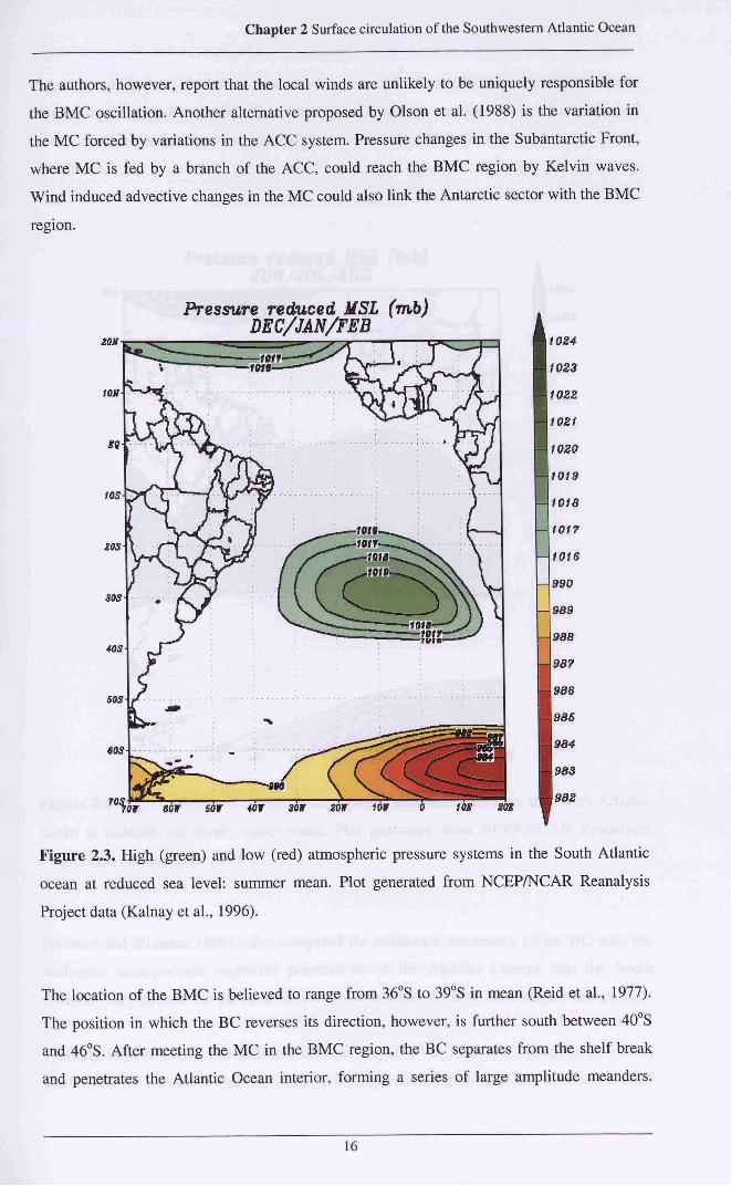
To illustrate the meteorological aspects of the South Atlantic ocean with respect to the
seasons, Figures 2.3 to 2.6 show the climatological atmospheric pressure and wind patterns at
reduced sea level and surface (1000 hPa), respectively, for the Austral summer and winter.
The maps were generated using selected data from the NCEP (National Center for
Environmental Prediction) / NCAR (National Center for Atmospheric Research) Reanalysis
Project (Kalnay et al., 1996), which contains the so-called "13-year base period monthly
means" valid for 1982 through 1994.
As described by Peterson and Stramma (1991), Figures 2.3 and 2.4 show the displacement of
the subtropical high pressure centre towards the north in wintertime. At the same time in
winter, the centre of this high increases in magnitude to about 1023 mb, whereas in summer
the highest pressure is about 1019 mb. The winds (Figures 2.5 and 2.6) are governed by the
distribution of the atmospheric pressure systems. In the BMC region the dominant winds are
from NW to W. Westerly winds achieve lower latitudes in wintertime. At the SBCS, on the
other hand, the dominant winds are coming from the NE and are weaker in the winter.
According to Olson et al. (1988), the local wind stress curl may also play a role in the position
where the BC separates from the coast (position sometimes interpreted as the BMC location).
15
Chapter 2 Surface circulation of the Southwestern Atlantic Ocean
The authors, however, report that the local winds are unlikely to be uniquely responsible for
the BMC oscillation. Another alternative proposed by Olson et al. (1988) is the variation in
the MC forced by variations in the ACC system. Pressure changes in the Subantarctic Front,
where MC is fed by a branch of the ACC, could reach the BMC region by Kelvin waves.
Wind induced advective changes in the MC could also link the Antarctic sector with the BMC
region.
Pressure reduced MSL (rob)DEC/JAN/FEB
eow sot r sow zow low
1024
1023
1022
1021
1020
1019
1018
1017
1016
990
989
988
98?
986
986
984
983
982
Figure 2.3. High (green) and low (red) atmospheric pressure systems in the South Atlantic
ocean at reduced sea level: summer mean. Plot generated from NCEP/NCAR Reanalysis
Project data (Kalnay et al., 1996).
The location of the BMC is believed to range from 36S to 39S in mean (Reid et al., 1977).
The position in which the BC reverses its direction, however, is further south between 40S
and 46S. After meeting the MC in the BMC region, the BC separates from the shelf break
and penetrates the Atlantic Ocean interior, forming a series of large amplitude meanders.
16

Chapter 2 Surface circulation of the Southwestern Atlantic Ocean
Legeckis and Gordon (1982) found the variable limit of 38S to 46S as the maximum latitude
of warm water related to the BC. The variability of this limit was found to be bi-monthly and
accompanied by intermittent formation of warm-core anticyclonic eddies.
20S
tos-
Pressure reduced MSL (mb)JVN/JUL/AUG
W BOT SOW 4OT SOW 20W WW 0 I OS 20E
1024
1023
1022
1021
1020
1019
iota
1017
10ie
990
989
988
987
986
985
984
98S
982
Figure 2.4. High (green) and low (red) atmospheric pressure systems in the South Atlantic
ocean at reduced sea level: winter mean. Plot generated from NCEP/NCAR Reanalysis
Project data (Kalnay et al., 1996).
Peterson and Stramma (1991) also compared the southward excursions of the BC with the
analogous semi-periodic westward penetrations of the Agulhas Current into the South
Atlantic. They pointed out the same bi-monthly time scales for both these current excursions.
Working with AVHRR data collected between July 1984 to June 1987, Olson et al. (1988)
established the statistical characteristics of the separation region from the continental shelf
17

Chapter 2 Surface circulation of the Southwestern Atlantic Ocean
(position of the crossing with the isobath of 1000 m) for both the BC and MC. Following
these authors, the BC separates from the shelf in the mean latitude of 35.8S, with a standard
deviation of 1.1, or about 210 km (the total range of latitudes was found to be 4.8, or 920
km). The MC, on the other hand, separates from the shelf at a mean latitude of 38.8S, with a
standard deviation of 0.9, or 170 km (the width of maximum separation is 4.4, or 850 km).
The band of separation between BC and MC was found to vary from zero to 6 in latitude.
ZOH
Wind (m/s) 1000 hPa - DEC/JAN/FEB
tos-
BQ-
tos
2QS
SOS
40S
t(( t t M f )f (M H t > , ,
w eow eon tor sow 2ow low o tos xos
10*
Figure 2.5. Surface winds in the South Atlantic ocean: summer mean. Plot generated from
NCEP/NCAR Reanalysis Project data (Kalnay et al., 1996).
18

Chapter 2 Surface circulation of the Southwestern Atlantic Ocean
Wind (m/s) 1000 hPa - JUN/JUL/AUGXON
tos
tos
zos
505
405
^ F Or 60W 40T SOW 2ÖW 1ÖW IDE 2ÖE
Figure 2.6. Surface winds in the South Atlantic ocean: winter mean. Plot generated from
NCEP/NCAR Reanalysis Project data (Kalnay et al., 1996).
2.5. Lagrangian measurements of currents and kinetic
energies
Several authors used drifting buoy measurements to describe either the large scale variability
of the Southern Hemisphere oceans or the mesoscale variability of the BMC region (e.g.
Patterson, 1985; Piola et al., 1987; Olson et al., 1988; Figueroa and Olson, 1989; Shafer and
Krauss, 1995). Satellite-tracked, drifting buoy data presented by Olson et al. (1988) show a
large anticyclonic circulation in the BMC region, believed to exist for long periods of time.
This anticyclonic cell is the one discussed earlier in this document (Section 2.3), which is
believed to participate in the process of intensification of the BC transport to the south of 30S
19

Chapter 2 Surface circulation of the Southwestern Atlantic Ocean
(Peterson and Stramma, 1991). One of the drifters presented in Olson et al. (1988) spent 8
months describing an anticyclonic circulation in the BMC area.
Schäfer and Krauss (1995) presented statistics for the major ocean currents in the
Southwestern Atlantic and in the ACC. The authors deployed more than 130 satellite-tracked
drifting buoys in the South Atlantic between 1990 and 1993, the majority of them drogued at
100 m depth. The BC mean velocity was found to be weak between 7S to 20S (4 cm/s 2),
increasing to 40 cm/s in the vicinity of the BMC region. The BMC region presented large
variability, with zonal and meridional r.m.s. (root mean square) currents of about 40 cm/s.
The South Atlantic Current (SAC) was found to be almost zonal, with less variability than the
BMC region, and presenting a mean velocity of 12 cm/s. The ACC in the Drake Passage and
Scotia Sea presented a mean eastward velocity of 16 cm/s, with high r.m.s. velocities
comparable to those from the BMC region. Following Schäfer and Krauss (1995), the BC
shows typical Eddy Kinetic Energy (EKE) varying between 200-400 cmV. The MC reaches
more than 500 cmV. EKE values in the BMC region reach 1600 cmVs2, decreasing again in
the SAC farther east.
Piola et al. (1987), Stevenson and Souza (1994) and Stevenson (1996) also presented EKE
values for the BC derived from drifting buoy data. While Piola et al. (1987) worked with
FGGE (First GARP Global Experiment) buoys, the last authors used WOCE standard LCD
drifters. EKE dominated the BC flow in both cases, but Stevenson and Souza (1994) and
Stevenson (1996) found these values to range between 1332 cm2/s2 and 4207 cmVs2, while
Piola et al. (1987) found 500 cm2/s2. The Mean Kinetic Energy (MKE) in the BC was
estimated to vary between 114-171 cm2/s2 by Stevenson and Souza (1994), values in good
agreement with 200 cmV found earlier by Piola et al. (1987). The value of 200 cm2/s2 was
also estimated for the MKE in the BMC region by Piola et al. (1987), but the EKE found in
this region was 1200 cm2/s2, much higher than in the BC.
2 Note that, despite recommendations for the utilisation of the International System of Units (SI), whichindicates m/s as the unit for expressing the speed, current speeds denoted in this thesis are in cm/s. The
units were previously used in the scientific literature described here and are kept for expressing our
results for the sake of a direct comparison with previous works. The same applies to the units of energywhich are here expressed in cni2/s2 instead of the SI unit J.
20

Chapter 2 Surface circulation of the Southwestern Atlantic Ocean
2.6. Brazil-Malvinas Confluence eddies
Eddies in the BMC region were first described by Legeckis and Gordon (1982) when
analysing the BC and MC in 1975, 1976 and 1978 from satellite infrared images. The authors
describe that the warm core eddies found at the BMC are formed during the retraction of the
BC from the confluence at intervals of a week. The eddies described by Legeckis and Gordon
(1982) for the BMC region are elliptical, with diameters of 180 km and 120 km for the major
and minor axis, respectively. Advection to the south is described to occur at velocities of 4
km/day to 35 km/day, the higher the velocity the younger the eddy would be.
Olson et al. (1988) described that the frontal region between BC and MC is filled with eddies
and high amplitude meanders. The authors have presented a very classical satellite image of
the BMC region (Figure 2.7), where a large elliptical warm core eddy (anticyclonic in the
southern hemisphere) of about 400 km by 200 km (major and minor axis respectively) is
noticed detached from the BC southward extension. Olson et al. (1988) also presented some
drifting buoys trajectories superimposed with AVHRR images in the BMC region to illustrate
the nature of an eddy and meanders of the MC/BC front.
Garzoli (1993), using inverted echo sounders at the BMC region, observed both cyclonic and
anticyclonic eddy circulation in the area. The author attributed the variability of the dynamic
height field of the BMC region to the variation of the front position, its meandering and to
eddy generation. Eddy diameters, as observed by Garzoli (1993), varied from 100 km to 150
km. These sizes were considered to be two to three times bigger than the expected Rossby
radius of deformation for the area.
By using the chemical tracer CFC-113, Smythe-Wright et al. (1996) identified an eddy
formed in the BMC region in the vicinity of Cape Basin, Africa (36.3S; 3.9E). Older than 4
years, approximately 600 m deep and measuring 150 km in diameter, the observation of this
eddy would have marked the first evidence of such a structure so far east in the South Atlantic
Ocean. Smythe-Wright et al. (1996) argue that this eddy should have travelled eastward in
isolation from the surface since November 1988, assuming a 5500 km long trajectory along
40S to 13E before turning northward in the far east part of the subtropical gyre. Although
the nature of this particular eddy has been recently claimed by McDonagh and Heywood
(1999) to be related to the Agulhas Current rather than to the BC, the final conclusions drawn
by Smythe-Wright et al. (1996) are still worth mentioning.
21

Chapter 2 Surface circulation of the Southwestern Atlantic Ocean
Figure 2.1. AVHRR image of the Brazil-Malvinas Confluence zone obtained in February
1985. The image illustrates the formation of a large anticyclonic (warm) eddy which had
detached from the Brazil Current (in red) at its southward extension. Malvinas Current waters
are seen in green to blue tones. Source: Olson et al. (1988).
Following the suggestion made by Gordon (1989) that at least 6 eddies are formed at the
BMC each year, and considering that some of these structures can reach the far east part of
the subtropical gyre, Smythe-Wright et al. (1996) suggested that the transport of multiple
eddies generated in the BMC region by the SAC serves to retain salt within the gyre. This
phenomenon would reduce the warm salty Indian Ocean water inflow required to balance the
overall salt budget of the subtropical South Atlantic. Smythe-Wright et al. (1996) also point
out the necessity of a systematic study of the characteristics of both the eddies formed at the
BMC region and at the SAC itself.
Hooker and Brown (1996) discussed the nature of BC eddies formed in the BMC region. For
the first time in the literature, the authors suggested that some of the BMC eddies are not
isolated monopole vortices, but have sometimes a dipole configuration for both warm and
cold rings. Hooker and Brown (1996) also observed a coalescence mechanism originated
from the interaction between a monopole (solitary) and a dipole eddy, pointing out the
22

Chapter 2 Surface circulation of the Southwestern Atlantic Ocean
importance of such a process since coalescence between two rings of opposite vorticities
cannot occur if they are both monopoles (one of them must be a dipole).
Hooker and Brown (1996) described dipoles formed in the BMC region lasting for 2 months,
rotating at a rate of about 12 degrees per day. The authors also called attention to the
importance of the use of infrared satellite imagery for studying the oceanic mesoscale
variability, and to the application of new methods of visualisation of AVHRR images to better
enhance the existence of dipoles in the ocean.
According to Podestä (1997) the present knowledge of the eddies in the Southwestern
Atlantic Ocean is still lacking in basic aspects such as the frequency of formation, typical
sizes, movements, lifetime and destination of these structures. Podestä (1997) hints that the
number of eddies expelled from the BC is lower than that of other western boundary currents,
but offers no proof for his affirmation. The energy contained in the BC eddies, however,
seems to be similar to that of eddies formed in more energetic currents (Olson, 1991; cited by
Podestä, 1997).
Podestä (1997) also reports that most of the studies based upon satellite data in the
Southwestern Atlantic are in fact related to the open ocean BMC region. The author points out
that, although there are many processes associated with the SST fields in the coastal regions
of the Southwestern Atlantic, the utilisation of satellite information for the monitoring of
these processes is not very frequent.
The results to be shown in this thesis offer an improvement to the present knowledge of the
mesoscale processes in the Southwestern Atlantic by combining satellite information with
drifting buoy data. Together with a study of the BMC region, a study of the SBCS and of the
eddy field of both these regions is offered here. Before presenting these results, however, the
next Section of this thesis will describe the basic concepts and historical development of the
SST observation and estimation through sensors onboard satellites.
23

Chapter 2 Surface circulation of the Southwestern Atlantic Ocean
BLANK PAGE
24

CHAPTER 3
SATELLITE OBSERVATIONS OF THE OCEAN
3.1. Historical perspective
Satellites have been used for several decades to observe physical processes in the upper layer
of the oceans. Remote Sensing offers synoptic views and regular temporal sampling of the
ground. Not considering the instrument and spacecraft conception and launching, Remote
Sensing data can be available at relatively low cost for the user. Remotely sensed data are
used to monitor small to large scale processes in the ocean, from coastal, shallow waters, to
deep ocean basins.
In comparison to the rest of the World Ocean, the Southwestern Atlantic is a region where
there is a huge lack of in situ measurements, specially those referring to currents (Campos et
al., 1996a; Peterson et al., 1996; Müller et al., 1998). As this is a chronic problem several
authors have used Remote Sensing data and techniques to increase their understanding of the
physical processes happening in that area.
Olson et al. (1988), for instance, report that the region of the Brazil-Malvinas (Falklands)
Confluence (BMC), inside the Southwestern Atlantic Ocean is particularly suited for studies
involving Remote Sensing techniques. The reason for this is the synoptic monitoring needed
to describe the spatial mesoscale variability of the BMC, and the strong thermal signal found
at the surface in that region.
Podesta (1997) points out that the strong thermal gradients between the Brazil and Malvinas
currents is the reason why the BMC region has been studied by remote sensing techniques
since the seventies. Tseng (1974) was pioneer on describing the BC fluctuations using
Remote Sensing. This author used infrared data from the infrared radiometer THIR
(Temperature Humidity Infrared Radiometer), which flew on the American satellite Nimbus-
5.
25

Chapter 3 Satellite observations of the ocean
The development of operational orbital platforms for studying the ocean derived mainly from
the American experience with the Mercury mission, in the sixties, and with the establishment
of the first series of Nimbus and NOAA (National Oceanic and Atmospheric Administration)
series of meteorological satellites, in the seventies. The NOAA series supported the
development of the Very High Resolution Radiometer (VHRR), an instrument designed to
assess the Sea Surface Temperature (SST) of the oceans. Further development of the VHRR
gave way to the modern AVHRR (Advanced Very High Resolution Radiometer), a present
day five channels instrument widely used to generate SST charts.
Meanwhile, in the nineties, an initiative of the European Space Agency (ESA) put in orbit the
ERS-1 (European Remote Sensing Satellite). Among other instruments, the ERS-1 satellite
carried onboard the ATSR (Along-Track Scanning Radiometer), which was designed to
measure the sea "skin" temperature, which is related to the first molecular layer of the sea at
the sea-air interface. In April 1995, the launching of the ERS-2 put in orbit the ATSR-2
instrument.
In August 1996, the Japanese Space Agency NASDA launched the ADEOS (Advanced Earth
Observing Satellite), carrying onboard the OCTS (Ocean Color and Temperature Scanner),
designed for coastal and oceanic investigation. ADEOS stopped transmitting data from 30
June 1997 onwards due to an operational failure. While the satellite was still operational,
however, OCTS was able to provide very good observational data for the oceanographic
community. OCTS was a 12 band, multi-spectral scanner, able to determine the Sea Colour
and SST at a spatial resolution of 700 m, better than both AVHRR and ATSR.
The study of ocean colour from space started in the late seventies with the deployment of the
Coastal Zone Colour Scanner (CZCS) onboard the NOAA Nimbus-7 satellite. This
instrument consistently recorded data in the World Ocean in order to achieve a measure of
the concentration of phytoplankton and to establish global seasonal levels of primary
productivity.
Following the success of the CZCS, NASA (National Aeronautics and Space Administration)
was planning for many years to launch another radiometer designed to measure the sea
colour. After years of expectations by the scientific community, the Sea-WIFS sensor was
finally launched in August 1997 onboard the SeaStar satellite. Although Sea-WIFS was
placed in orbit a little later than OCTS, the malfunction of the ADEOS satellite made Sea-
WIFS the only sea colour orbital scanner in operation until May 1999.
26

Chapter 3 Satellite observations of the ocean
Owing to the general interest of the scientific community in the sea's primary production
estimated from sea colour data, the Indian Space Research Organization (ISRO) launched its
own sea colour orbital sensor, the OCM (Ocean Colour Monitor) on 26 May 1999. This
instrument is a solid state camera operating in eight spectral bands flying onboard the IRS-P4
(Oceansat-1) satellite.
During the last decades both the end of the cold war and the necessity for new variables to be
monitored in the oceans allowed civil space enterprises to develop and to launch other kinds
of sensors into space. The use of radar imagery or altimetry in oceanography, for example, is
nowadays widely applicable to the study of surface and internal waves, surface slicks, bottom
topography, surface winds, geostrophic currents and sea level. The first orbital radar images
produced over the ocean were obtained by the Seasat satellite, launched in 1978 and alive for
about 100 days. The results of its Synthetic Aperture Radar (SAR) were very remarkable, and
it was used later as the base of the modem SARs.
Seasat was also designed to establish the "proof of concept" for ocean circulation
measurements by a radar altimeter (Yamarone Jr. et al., 1995). Due to its good results and to
the results of other missions (e.g. the Skylab, GEOS-3 and Geosat), the United States and
France established plans for what became the joint mission TOPEX (Ocean Topography
Experiment) / Poseidon (T/P). Since its launching on 10 August 1992, the T/P satellite has
been measuring the height of the sea surface relative to the Earth's centre of mass, which
allows the mapping of the ocean's topography. Other geophysical parameters like geostrophic
currents, tides and waves, for example, can also be studied by utilising T/P measurements.
Following the same principles of T/P, ESA is currently also running its own altimetry
mission onboard ERS satellite series.
As discussed, the satellite and instruments designed to retrieve physical parameters of the
ocean in a global or local basis are many. In the context of this thesis, where the AVHRR and
ATSR instruments are used to provide SST estimates over the study region, the
characteristics of these sensors and their carrying platforms will be better described in the
next sections.
27

Chapter 3 Satellite observations of the ocean
3.2. Thermal infrared imagery
3.2.1. Satellites and sensors
The establishment of a series of procedures leading to the estimation of SST from satellite
measurements began in the early sixties with the operation of the Television Infra Red
Observational Satellites (TIROS). The meteorological TIROS Operational Satellites (TOS)
operated between 1966 and 1969, leading to the Improved TIROS Operational Satellites
(ITOS) series in the early seventies.
The ITOS series of satellites were taken over afterwards by NOAA, being renamed as the
TIROS/NOAA series. From 1978, NOAA started the Advanced TIROS-N (ATN) series,
which has been in continuous operation until the present (Forrester, 1991; Kidwell, 1995).
The last version of the radiometer carried by the NOAA satellites is the AVHRR/2, referred
to here simply as AVHRR, although AVHRR/3 is expected by the beginning of this decade.
In 1991, ESA launched the ERS-1, which carried the ATSR sensor. This instrument is
composed of a passive Infrared Radiometer (IRR) and a two-channel (23.8 and 36.5GHz)
Microwave Sounder, aiming to provide atmospheric total water vapour content. Further
references in this text to the ATSR are actually relative to the IRR. The nature of the SST
estimate performed by the ATSR is intrinsically different from that of AVHRR, since the
ATSR instrument is designed to make conical scans over the scene, in two distinct angles of
view (discussed later in this section). Based upon the success of the ERS-1 mission, ESA
launched the ERS-2 satellite in 1995, putting the ATSR-2 sensor in orbit. Following this,
ESA plans to launch the AATSR (Advanced ATSR) on Envisat early this decade.
All NOAA series and ERS satellites fly sun-synchronous (quasi-polar) orbits around the
earth, approximately at an altitude of 800 km. NOAA manages to operate 2 satellites
simultaneously, separated by about 90 in longitude (about 6 hours), which means there are at
least four overpasses at each location daily, a much better temporal resolution than ATSR.
The ascending node for NOAA-11, 13 and 14 satellites was set to 13:40 LST (Local Solar
Time), while the descending node was set to 01:40 LST. NOAA-12 is orbiting its ascending
node at 19:30 LST and its descending node at 07:30 LST. This satellite is nowadays
operating simultaneously with NOAA-14, but some years ago NOAA-12 used to operate with
NOAA-11.
28

Chapter 3 Satellite observations of the ocean
The temporal resolution of ATSR images depends mainly on the ERS orbit phase and cloud
coverage. Jones (1997) shows the sampling density of ATSR data in the South Atlantic ocean
for the period between January 1992 and December 1994. Due to the increase of cloud
coverage towards the pole, Jones (1996) found a typical sampling density of two
measurements every 10 days in the tropics, and of 1 measurement every 20 days at higher
latitudes. All the polar-orbiting satellites with sensors able to estimate SST in operation
during the years of 1993 and 1994 (the period when the drifters used in this study were at the
sea) are shown in Table 3.1.
The spectral channels for AVHRR and ATSR sensors are centred at the following
wavelengths:
- 0.63 m (AVHRR channel 1);
- 0.91 m (AVHRR channel 2);
- 1.6 m (ATSR-1 channel 1);
- 3.7 m (AVHRR channel 3; ATSR-1 channel 2);
- 10.8 m (AVHRR channel 4; ATSR-1 channel 3);
- 12 Mm (AVHRR channel 5; ATSR-1 channel 4).
The AVHRR instrument has its first two channels centred at visible (suitable for cloud
identification) and near infrared (suitable for land/sea discrimination) bands of the
electromagnetic spectrum. Aiming to improve daytime cloud identification over snow and
ice, the ATSR instrument has an unique channel in the near-infrared substituting both
AVHRR channels 1 and 2 (Zavody et al., 1994). ATSR-2, on the other hand, has added three
visible channels in comparison to ATSR-1, those centred at 0.56 m, 0.67 m and 0.87 m.
The AVHRR sweeps out a swath of about 3000 km wide on the earth's surface, the product
of a cross-track field of view (FOV) of 54 off nadir. Full-resolution (1.1 km at nadir) data
are automatically downloaded to the ground stations in the HRPT (High Resolution Picture
Transmission) mode. From the total time of about 102 min of each satellite orbit, 10 min of
full-resolution data can also be recorded onboard and later downloaded to one of CDA
(Command and Data Acquisition) ground stations managed by the NOAA NESDIS (National
Environmental Satellite, Data and Information Service). This mode of acquisition is named
LAC (Local Area Coverage).
29

Chapter 3 Satellite observations of the ocean
Table 3.1. Satellite and sensors operating between 1993-94
satellite
NOAA-11
NOAA-12
NOAA-13
NOAA-14
ERS-1
satellite lifetime24 September 1988 -
11 April 199514 May 1991 -
present9 August 1993 -
21 August 199330 December 1994 -
present17 July 1991 -
2 June 1996
sensor
AVHRR
AVHRR
AVHRR
AVHRR
ATSR-1
sensor lifetime8 November 1988 -
11 April 1995
same as the satellite
same as the satellite
11 April 1995-present
3.7 m channel failed on
26 May 1992
When NOAA satellites dump the full-resolution data to the ground, an internal recorder also
re-samples this acquired data from 1 km x 1 km to 4 km x 4 km resolution. By doing that, the
system allows the CDA stations to receive the complete (re-sampled) set of data registered at
each entire satellite orbit. This acquisition mode is known as GAC (Global Area Coverage),
and is the basis of NOAA's global operational SST charts, such as the NOAA MCSST
products and, more recently, the NOAA AVHRR Oceans Pathfinder (Forrester, 1991,
Vazquez et al., 1998).
The modes of acquisition and downloading of ATSR images are slightly different from
NOAA's.ATSR is a radiometer with a conical scan (Figure 3.1), inclined at angles varying
from 0 to 24 in the nadir view, and from 53 to 55 in the forward view (Saunders et al.,
1993; Mutlow et al., 1994; Jones, 1997). Pixel resolution ranges from 1 km x 1 km at nadir to
1.5 km x 2 km at 55. The ATSR curved swath is nominally 500 km wide, with 555 pixels
across the nadir swath and 371 pixels across the forward swath (Mutlow et al., 1994).
Due to its telemetry bandwidth, the ATSR data need to be compressed onboard the satellite
before its downloading to the ground. This compression procedure allows three out of the
four ATSR channels to be transmitted simultaneously. Two of the three telemetry slots are
always occupied by ATSR channels 3 and 4. The third telemetry slot transmits either channel
1 or channel 2 data, depending on an automatic selection based on the scene radiance levels
measured by channel 1. The automatic selection generally results in the transmission of
channel 1 data in the daytime, and of channel 2 data at night. Nevertheless, bright spots in the
scene at night produced by forest fires, as an example, can trigger the transmission of channel
1 data (Mutlow et al., 1994).
30

Chapter 3 Satellite observations of the ocean
Zavody et al. (1994) discuss the ATSR processing scheme developed at the UK Earth
Observation Data Centre (EODC), including the modes of decodification of telemetry data,
geolocation of the images and derivation of scientific products, such as the SST images.
According to Zävody et al. (1994), geolocation is by far the most complex part of the ATSR
processing scheme. Images produced by the ATSR conical scan are mapped into 1 km x 1 km
pixels in two-dimensional 512 x 512 arrays, and collocation accuracy of both nadir and
forward view 512 km x 512 km images is about 1 km in the worst case. SST products
available from ATSR measurements include the full-resolution (512 X 512 array, 1 km x 1
km pixel resolution) data, and a high precision, global, spatially averaged SST field (Mutlow
et al., 1994). This last product, called ASST, is produced by cloud clearing and the averaging
of full-resolution data into sample bins of 0.5 degrees x 0.5 degrees in latitude/longitude.
Flight Direction
ATSRInstrument
Sub-satellite Track
Nadir view swath
(555 nadir pixels1 km resolution)
Forward view swath
(371 along track pixel1,5 km x 2 km resolution \
Figure 3.1. ATSR scan geometry. Source: Mutlow et al. (1994).
31

Chapter 3 Satellite observations of the ocean
Infrared radiometer measurements are expected to be accurate, requiring the sensors to be
well calibrated and stable. Following Planck's Law (see Section 3.2.2), small errors in
radiance measurements made by the sensors can generate large errors in retrieving the actual
temperature of the scene (Robinson, 1985). Long-term, onboard calibrations of the ground
radiance measurements are often made by taking onboard blackbody radiance measurements
as well. Both AVHRR and ATSR are designed to make measurements on temperature-stable
(warm) internal blackbodies and on the (cold) space every scan cycle. The use of linear
extrapolation between digital counts of blackbody or space radiance, and ground radiance is
used to retrieve ground digital counts.
Robinson (1985) reports that AVHRR in-flight calibration errors can produce temperature
uncertainties of about 0.3 degK. This arises from errors in the assumed emissivity of the
blackbody, and from the accuracy and resolution of the platinum resistance thermometers
used to monitor the blackbodies' temperatures. Saunders et al. (1993) consider the ATSR
able to make improved retrievals of temperature over the AVHRR, because of its greater
capability to correct for atmospheric effects, an accuracy of onboard absolute calibration of
less than 0.1 degK and a lower system noise temperature (< 0.05 degK). Mutlow et al. (1994)
note that the accuracy on the ATSR retrieved temperatures does not depend primarily on the
calibration of the instrument.
Pre-launch tests made on the AVHRR instrument are also performed in order to determine
coefficients to account for the non-linearity in the AVHRR channels 4 and 5 response. Non-
linearity arises in these two channels because of the HgCdTe detectors response to radiance.
AVHRR channel 3, which uses an InSb detector, has a highly linear calibration. After launch
of the instrument, the non-linear corrections are appended to on-board calibrations made with
the blackbodies and assuming a radiance of space (Nsp) equal to zero. According to Kidwell
(1995), the non-linear corrections assuming Nsp as zero is valid for NOAA-9, 10, 11 and 12
spacecrafts. For NOAA-13 and successors, NOAA is providing a correction scheme which
uses the Nsp value as negative instead of zero. As one of the advantages of this new scheme,
the AVHRR data user is now able to choose to correct either the radiance or the brightness
temperature data. Besides, this scheme is being applied retrospectively in the NOAA/NASA
Pathfinder Program to generate a consistent time series of NOAA radiances from 1981 to the
present for use in studies of climate (Kidwell, 1995).
32

Chapter 3 Satellite observations of the ocean
3.2.2. Sea surface temperature estimates
Infrared radiometers are instruments designed to measure the infrared radiation reflected or
emitted by the earth surface towards the direction of the sensor. Although the sun emits
radiation at shorter wavelengths peaking in the visible (0.4 m to 0.7 m), the earth emits
radiation peaking around 10 m, which is thermal infrared. The amount of energy emitted by
the sea surface towards the direction of an infrared radiometer mounted on a satellite orbiting
the earth is the basis for computing the SST.
Robinson (1985), Maul (1985) and Fiuza (1992) offer excellent texts regarding the physics of
the infrared radiation and its relation to the "real" temperature of a "grey" body. The
relationship between Spectral Exitance (or Spectral Emmitance, M%) and Temperature (7) of
a perfect emitter blackbody is given by Planck's Law:
Mx = LxTZ = r-^
: 11 (T6 (3.1)X5[{ClXr)\]X5[exp{CilXr)-\]
where:
M\\ Spectral exitance in
L\: Spectral radiance in
X: Wavelength in m;
Ci:3.74.10"16W.m"2;
C2: 1.44.10"2m.degK;T: Temperature in degK.
Planck's Law assumes that the blackbody is a Lambertian surface (emits radiation equally in
all directions). The relation between the Spectral Exitance of a blackbody (perfect emitter)
and a grey body (natural surfaces) is given by the Spectral Emissivity (Ex):
_Mxnatural surfaceMx blackbody
33

Chapter 3 Satellite observations of the ocean
The emissivity does vary weakly in relation to the body's temperature, but major variations
are caused by varying the wavelength. Sea surface emissivity is about 0.98, varying very little
with wavelengths between 3 m to 14 m (range of infrared sensors), temperature and
surface roughness, although affected by surface slicks (Robinson, 1985). Satellite Zenith
Angle (SZA) also plays an important effect in the sea surface emissivity and, at SZA equal or
greater than 50, waves are likely to produce some effect as well. Sensors measuring the 3.7
m channel (AVHRR channel 3 and ATSR channel 2) were found to have daily infrared
radiance measurements contaminated by direct solar irradiance reflected at the sea surface.
As a result of this, AVHRR channel 3 and ATSR channel 2 are only used in night algorithms
to produce SST estimates.
Having measured L% by different channels of each infrared radiometer, Equation 3.1 enables
one to compute the scene temperature as if the emitter was a blackbody. This wavelength
dependent temperature is called "apparent" or "brightness" temperature (BT), and it forms
the basis of empirical or experimental algorithms to generate SST.
Although the infrared radiometers are designed to operate in certain bands (channels) of the
electromagnetic spectrum where the influence of the atmosphere is lower ("atmospheric
windows"), the pathlength of atmosphere between the ground and the orbital sensor still
influences the level of radiance detected by the sensor. Robinson (1985) observes that
absorption of incoming radiation and later re-emission of it in different wavelengths is the
main problem in the spectral range of 3 ^i to 14 m. In opposition to the visible, infrared
radiation is less affected by molecular or aerosol scattering. Robinson (1985) also refers to
ozone, carbon dioxide and water vapour as the main absorbers of infrared radiation in the
atmosphere. Zavody et al. (1995) also consider the following gases as minor contributors to
the absorption in the atmosphere: nitrogen, nitric acid, ammonia, carbonyl sulphide, nitrous
oxide, methane, trichloromethane (FC11) and dichlorofluoromethane (FC 12).
The actual absorbance of the atmosphere varies both spatially and temporally, and the
distribution of its absorbing molecules through the atmosphere varies in an even more
complicated manner. The result, however, is that the atmosphere (being cooler than the
ground or sea) emits infrared radiation representing lower temperatures than the ground or
sea.
The AVHRR and ATSR programmes have different approaches to solve or diminish the
effect of atmospheric absorption. From the development of the AVHRR sensor, the approach
34

Chapter 3 Satellite observations of the ocean
to estimate SST from infrared measurements was a multi-channel or multi-window technique,
where different BT measurements taken on different channels in the infrared are combined in
a specific algorithm. The first AVHRR/2 (5 channels) instrument launched onboard NOAA-7
allowed the establishment of the MCSST (Multi-Channel Sea Surface Temperature)
procedure.
The MCSST procedure, obtained by regressing different pairs of combinations between two
or three AVHRR infrared channels, resulted in simulation equations with very small errors of
SST prediction (McClain et al., 1985). When compared with in situ SST data, however, the
equations proved to have a consistent bias. In order to reduce this bias, NOAA started to use
sets of closely matched buoy and satellite measurements. As a result, NOAA's algorithms
evolved to estimate subsurface "pseudo-bulk" temperatures (close to those measured by
buoys or ships of opportunity), rather than the "skin" temperatures from which the radiance is
directly emerging towards the sensor. McClain et al. (1985) also indicate that the addition of
terms depending upon the Satellite Zenith Angle (SZA) gave better performance to the
nighttime MCSST algorithms. The authors also indicate that SST estimates retrieved by the
MCSST scheme have accuracies of 0.5-0.6 degK. An extensive description of all atmospheric
correction algorithms used so far at NOAA since the launching of the TIROS-N spacecraft in
1978 can be found in Kidwell (1995).
ATSR measurements, on the other hand, can be combined in terms of different angles of
viewing the same scene. This technique, known as the multi-view technique, allows
correction for the atmospheric effect by estimating the influence of the absorbers through
different atmospheric paths. The way of combining different channels in different views are
similar to NOAA's "dual-window", "split-window" or "triple-window" techniques, although
the retrieved temperature refers to the "skin" or molecular surface of the sea. Differences
between "bulk" and "skin" temperatures are still under investigation, and some discussions
on this subject can be found in Robinson (1985), Hepplewhite (1989), and Mutlow et al.
(1994), among others. Zavody et al. (1994) report this problem as a work in progress to
provide further enhancements of the ATSR data products.
35

Chapter 3 Satellite observations of the ocean
BLANK PAGE
36

CHAPTER 4
DATA AND DATA PROCESSING METHODS
4.1. Low Cost Drifters
4.1.1. Characteristics of the buoys and associated data
The drifting buoys used in this work were built at INPE (Institute Nacional de Pesquisas
Espaciais - National Institute for Space Research), Brazil, for use in the COROAS project, the
Brazilian counterpart to the WOCE project (Campos et al., 1996). Like all the surface drifters
in use within the WOCE Surface Velocity Program (SVP), the COROAS LCDs were
fabricated following the design proposed by Sybrandy and Niiler (1991).
The principal components of the LCDs are the surface float, the wire tethers, the subsurface
float or balance element and the holey-sock drogue (Figures 4.1 and 4.2). The surface float
houses the antenna, the Platform Transmitter Terminal (PTT, the ARGOS transmitter plus the
data processor), batteries and the SST and drogue-loss (immersion) sensors. The holey-sock
drogue provides the drag for the LCDs surface float. The LCD is designed to follow water
parcels vertically averaged over the holey-sock height of about 6-7 m, centred 15 m below the
surface (Niiler et al., 1991).
According to Niiler et al. (1991), the LCD design was developed to meet two principal
objectives:
To have known water-following characteristics or to have a predictable slip of the drogue
centre through the water (for the water-following capability of the holey-sock drogue refer to
Niiler et al. (1995));
To last for many months in the rugged open ocean environment.
A third objective of the design, as the name of the drifter indicates, is the low cost of its
fabrication (around US$ 2000 in 1991). The facility of deployment was also desirable.
37

Chapter 4 Data and data processing methods
Figure 4.1. Photograph of the WOCE standard Low Cost Drifter (LCD) fabricated at INPE.
The drifter design adopted by the SVP/WOCE attempted to minimise the effects of wind and
waves in the surface float, the contamination of the current signal by aliasing of wave-induced
and tether forces, and slippage of the drogue. To achieve that, the LCDs have some distinct
mechanical characteristics (Sybrandy et al., 1995):
The surface float is spherical in order to minimise the rectification of surface waves into
net horizontal forces;
A subsurface float is present to reduce the mean tension between the surface and subsurface
components. This also reduces the aliasing of vertical forces into slip-producing horizontal
forces;
The wire tethers are thin and stiff in order to minimise drag-induced slip and to reduce
looping and kinking caused by wind waves;
The drogue is dimensionally stable with a design resistant to kiting under normal load
conditions. The holey-sock gives a drag area ratio (drogue:tether + floats) of about 37.
The ARGOS PTTs contained in the COROAS drifters were programmed to report
geophysical parameters to the NOAA satellites at 90 second intervals. In order to save energy
and costs, the PTTs were also programmed to work only for 8 hours per day.
38

Chapter 4 Data and data processing methods
1500 cm
644 cm
92 cm
Figure 4.2. Squematic of the LCD. Source: Sybrandy and Niiler (1991).
To be able to measure SST, each LCD had a thermistor attached to the hull. The thermistor
measured temperatures at 12 cm beneath the mean water line of the buoy to a precision of
about 0.05C (Stevenson et al., 1998). The buoys' positions, together with the temperature
measurements and other geophysical parameters (such as the battery level and an empirical
39

Chapter 4 Data and data processing methods
measurement of whether the buoy still had its drogue, for instance) were assessed through the
ARGOS System at CNES (Centre National d'Etudes Spatiales) in Toulouse, France.
The drifters' positions were computed in the ARGOS centre in Toulouse. At the time our data
were acquired, ARGOS used to compute the location of moving PTTs by using the
measurement of the Doppler effect on the transmitters' signals to the satellites during their
passage above the transmitters' horizon (ARGOS, 1988).
The accuracy of the location estimates made at ARGOS in the past were divided into three
different classes, where the best, used in our data, was nominally equal to 150 m (ARGOS,
1988). Depending on the quality of data being transmitted and external factors like the sea
state, for example, the locations could in fact be accurate to 111 m or 0.001 in latitude
(Stevenson et al., 1998). At the time of writing, however, ARGOS-tracked platforms are
being configured to transmit GPS (Global Positional System) data together with their
geophysical measurements, which has improved the accuracy of the locations to circa 5 m.
Owing to the previous ARGOS methodologies of retrieving the PTTs' locations, only one
position for each LCD was computed for each particular NOAA satellite overflight above the
transmitter horizon. To assure good quality data as well, ARGOS also only compute a
particular location if more than 3 transmissions are received during the overflight (Stevenson
et al., 1998). The same is not the case for the geophysical parameters being measured by the
buoys, like temperature. Because the measurements are transmitted to the satellite at 90 s,
several of them are actually received by the satellite during each overpass. The result is that
the user ends up with more temperature measurements than buoy locations in relation to the
time.
The duration of a particular NOAA satellite overflight above a transmitter located at the sea
surface is about 10 to 15 minutes. The number of NOAA satellite overflights in a particular
location, though, increases with latitude. That makes the number of locations obtained by
ARGOS for a particular PTT increase with latitude as well. Stevenson and Alonso (1986)
have shown that the number of ARGOS locations per day is around 6 between the Equator
and 40 in latitude, increasing exponentially to 19 at the latitude of about 70N or 70S.
After the collection phase, the LCD data were retrieved from the ARGOS centre in France to
INPE, Brazil, through a modem connection. Each LCD time series was recovered and updated
at 4 day intervals until the end of the transmission period for each buoy. Once all the time
40

Chapter 4 Data and data processing methods
series were complete, the data were submitted to a test of consistency, which discarded
discrepancies in both position and temperature series.
To overcome the problem of receiving more temperature measurements than buoy locations,
the temperature data used in this work was always the one closer in time (usually zero to a
few seconds) to a particular buoy position computed by ARGOS. No temporal temperature
average was performed for a given overflight also because the buoys were most of the time
following temperature contours which do not change in the very short period of time typical
of a satellite overpass and, by consequence, most of the temperature retrievals were the same.
Very few exceptions to that were treated case by case and spurious data were visually
discarded from the series.
The drifters used in this work were deployed in the BC in a position close to the shelf break
near 24.8S, 44.3W off the Säo Paulo State coast, Brazil. The deployment campaign was
conducted by the COROAS project, onboard the R.V. Prof. W. Besnard. The buoys were
deployed following a box pattern, five at a time, in February 1993 (buoys number 3178 to
3182), July 1993 (number 3183 to 3187) and January 1994 (number 3188 to 3192). For more
information about the LCDs' launching procedure refer to Stevenson and Castro Filho (1996).
Following the general flow of the BC, the 15 buoys launched in this current drifted
southwestward covering the COROAS region of interest off the Säo Paulo coast (~ 23S to
27S, 42W to 47W). From the second group of buoys launched in the BC, buoys 3184 and.
3186 stopped transmitting data immediately after the launching. All the other 13 buoys
traversed the COROAS study area. After a variable time which depended on each particular
buoy trajectory, all the buoys (apart from buoy 3183) reached the vicinity of the BMC region
at about 30S. The BMC area not being a region of primary interest for COROAS objectives,
the Lagrangian dataset collected by the project in that area was kindly made available for this
research.
The Lagrangian dataset used in this work, then, consists of positions and temperature time
series of 12 LCDs which had drifted into the vicinity of the BMC region in 1993 and 1994.
The lifetime period of each LCD depended on both the PTTs electronic programming scheme
and on eventual accidental losses. Without counting the time already spent in the COROAS
area of study, the buoys used here had lifetimes varying from 2 weeks to about 11 months
(Table 4.1.).
41

Chapter 4 Data and data processing methods
Table 4.1. Lifetime and number of observations (N) for the LCDs
after achieving the vicinity of the BMC region
buoy3178
317931803181318231853187
31883189
31903191
3192
start (Julian day)6 Apr 93 (96)24 Mar 93 (83)21 May 93 (141)12 Mar 93 (71)23 Mar 93 (83)1 Set 93 (244)13 Dec 93 (347)12 Feb 94 (408)13 Feb 94 (409)5 Feb 94 (401)1 Feb 94 (397)4 Feb 94 (400)
finish (Julian day)3 Jul 93 (184)15 Oct 93 (288)30 Jul 93 (211)26 Mar 93 (85)11 Feb 94 (407)15 Apr 94 (470)16 Apr 94 (471)1 Mar 94 (425)5 Jul 94 (551)5 Jul 94 (551)5 Jul 94 (551)5 Jul 94 (551)
lifetime (days)88.03
204.2969.7814.27
324.23226.03
123.1117.03141.96150.05153.99
151.03
N
186298224
21
1350747
37165513474
576585
Note: Julian day l = 1 Jan 93; Julian day 366 = 1 Jan 94.
After reaching the area close to the BMC region at about 30S in the BC, three LCDs turned
westward, penetrated the continental shelf and then drifted in a direction opposite to the BC
flow. Previous COROAS results suggested a coastal recirculation scheme for the BC
(Stevenson and Souza, 1994; Stevenson, 1996), in which the northeastward course followed
by these buoys was thought to be a coastal branch of a large BC loop. Further analysis made
in this work (Chapter 6) has demonstrated that the buoys actually entered a coastal current
which interacts with BC, but which is not part of it. This current is referred to in this work as
the Brazilian Coastal Current (BCC).
Seven of the remaining LCDs followed an eastward direction when reaching the BMC region.
Carried by the extension of BC called the South Atlantic Current (SAC), these buoys
penetrated the open ocean to longitudes up to 36W. The other 2 LCDs used here had
trajectories entirely located in the BC. None of the buoys used here sampled the Malvinas
(Falkland) Current. Figure 4.3 shows the overall trajectories of the LCDs in the form of a
'spaghetti diagram'.
The number of locations retrieved for each of the drifters used in this work varied from 0 to 7
per day, being equal to 4 most of the time (39.4 % of the cases). Figure 4.4 displays the
frequency histogram of the number of observations per day for the overall set of LCDs used
here. 86.7 % of the data were collected at the rate of 2 to 5 locations per day. Considering that
the range of latitudes covered by our LCDs was between 23S and 45S (Figure 4.3), 2 to 5
42

Chapter 4 Data and data processing methods
locations per day are broadly in agreement with the estimates made previously by Stevenson
and Alonso for Service ARGOS retrievals (1986).
-60 -55 -50 -45
longitude
Figure 4.3. Overall trajectories of the LCDs used in this work.
0 12 3 4 5 6 7number of locations per day
Figure 4.4. Frequency histogram of the locations per day for the LCDs.
43

Chapter 4 Data and data processing methods
4.1.2. Data processing
4.1.2.1. Pre-processing and quality control
As remarked before, the LCD time series were submitted to pre-processing and quality
control in order to discard eventual discrepancies in both position and temperature data.
First of all, part of the temperature data, more frequent than the positional data in the original
time series, was discarded following the procedure described in Section 4.1.1. Owing to the
technology involved in the telemetry link between the PTT and the satellite (transmission of a
UHF signal with the PTT identification and geophysical measurements), electronic noise is
often encountered. This causes the recording of spurious data. Other factors like the stability
of the PTT's internal oscillator (which mantains the transmission signal at a certain
frequency) or even its abrupt movement caused by the sea state, for example, can also cause
the apperance of bad data in the series. Spiking points in both the temperature and position
time series, when caused by bad data, were often several orders of magnitude bigger or
smaller than the adjacent points. They were manually discarded from all the time series. This
was preferable rather than aliasing of the series because the number of locations per day for
the buoys (Figure 4.4) was low and confined to a period of the day which depended on the
NOAA's satellites orbit.
4.1.2.2. Time series
After passing the quality control, their time series of latitude, longitude and temperature
collected by the LCDs were processed to compute the main characteristics in the Brazil
Current (BC), the South Atlantic Current (SAC) and the Brazilian Coastal Current (BCC).
The trajectories described by each particular buoy were described entirely in the BC (buoys
number 3181 and 3188), entirely in the BCC (3178 and 3180), in the BC and BCC (3179), or
in the BC and SAC (3182, 3185, 3187, 3189, 3190, 3191 and 3192). The data from all buoys
were divided into their BC, SAC and BCC components, in order to separately describe these
currents.
Since the BC develops its main flow as a western boundary current parallel to the coast
(southwestward in the BMC vicinity), the criteria adopted to divide each entire track into its
current components was based upon the southernmost location where a major change from
44

Chapter 4 Data and data processing methods
the BC direction occurred in the trajectories. In every case of a buoy leaving the BC and
entering the SAC, for instance, the change in direction was about 90 degrees, from SW to SE.
In the case of the buoy entering the BCC from BC, the change in direction was about 180
degrees, from SW to NW. Table 4.2 shows the time intervals and geographical positions of
the beginning and end of the series used to describe the BC, BCC and SAC.
4.1.2.3. Mean current and kinetic energies
To estimate the current speed and direction, all the buoy positions for a particular current
were transformed from longitude and latitude into zonal and meridional displacements,
respectively. Units were converted from the original degrees per day into cm/s. While the
international recommendation is to use the International system (SI) units, the CGS units were
used here in order to facilitate direct comparison with previously published results, essentially
all of which are in CGS units.
Table 4.2. Time series used to describe the BC, BCC and SAC
(a) Brazil Current
buoy3179
3181
3182
3185
3187
31883189
319031913192
buoy3178
3179
3180
date (Julian day)start
24 Mar 93 (83)12 Mar 93 (71)23 Mar 93 (83)1 Set 93 (244)13 Dec 93 (347)12 Feb 94 (408)13 Feb 94 (409)5 Feb 94 (401)1 Feb 94 (397)4 Feb 94 (400)
finish27 Apr 93 (117)26 Mar 93 (85)28 Mar 93 (87)24 Oct 93 (297)4 Jan 94 (369)1 Mar 94 (425)15 Mar 94 (439)1 Mar 94 (425)27 Feb 94 (423)26 Feb 94 (422)
(b) Brazilian Coastal
date (Julian day)start
6 Apr 93 (96)28 Apr 93 (118)21 May 93 (141)
finish3 Jul 93 (184)15 Oct 93 (288)30 Jul 93 (211)
laütudi
start
47.60
47.85
47.9047.8548.55
47.9148.2947.55.47.1947.49
Current
!(S)finish49.73
50.36
48.36
50.13
52.07
51.6253.2553.4652.9353.58
latitude (S)start
28.5930.93
33.30
finish23.1025.60
24.59
longitude (W)start
29.5229.82
30.15
29.9829.82
29.7929.9529.7929.62
29.95
finish31.09
32.53
31.0533.30
36.6634.1936.8037.5137.50
37.07
longitude (W)start
48.02
49.87
50.79
finish44.37
46.48
45.02
45

Chapter 4 Data and data processing methods
buoy31823185318731893190
3191
3192
(c) South Atlantic
date (Julian day)start
28 Mar 93 (87)24 Oct 93 (297)5 Jan 94 (370)15 Mar 94 (439)2 Mar 94 (426)28 Feb 94 (424)27 Feb 94 (423)
finish11 Feb 94 (407)15 Apr 94 (470)16 Apr 94 (471)5 Jul 94 (551)5 Jul 94 (551)5 Jul 94 (551)5 Jul 94 (551)
Current
latitude
start
48.3450.1252.0653.2553.44
52.8753.34
(S)finish38.9540.08
37.24
39.2747.43
41.9338.46
longitude (W)start
31.06
33.32
36.6936.8037.8537.83
37.70
finish31.19
33.51
37.9634.5839.6738.99
35.81
Having the zonal and meridional displacements (Xj, yO, and knowing the time interval (t)
between two consecutive position measurements (i, i+1), the zonal (0 and meridional (v;)
instantaneous velocities (cm/s) were computed as follows:
X.
(4.1)
The mean zonal (U) and meridional (V) velocity components for each time series were
given by:
_ t n-\_ !
n-\(4.2)
n~i=\
where n is the number of points in each positional time series.
The overall mean current velocity (V^) and the mean current direction (0C) were obtained
from:
Vm =2 2 V
Be = arctam = (4.3)
where Vm is in cm/s and 6C is in degrees. The final mean current direction, however, was
transformed into the appropriate geographic bearing.
In order to examine the influence of time dependent, mesoscale perturbations present in each
trajectory within the BC, SAC and BCC, the time series were also used to compute the mean,
eddy and total kinetic energies (MKE, EKE and TKE, respectively) as defined below. These
46

Chapter 4 Data and data processing methods
energies were computed on a temporal basis, in contrast with some methodologies which use
spatial averages (e.g. Figueroa and Olson, 1989; Zambianchi and Griffa, 1994; Schäfer and
Krauss, 1995). This approach has the advantage of computing energies for each buoy time
series, and is especially useful when one has a small number of tracks over a specific area or
if the study area is not regularly covered by the tracks.
For the computation of the kinetic energies, it was assumed that the velocity of a fluid parcel,
at a particular moment along its trajectory, was equal to the summation of the velocity of a
mean current (Vm) and of a perturbation. The instantaneous zonal (u\) and meridional (v'j)
perturbation velocities were represented by the successive buoy detrended (demeaned)
instantaneous velocities.
The mean kinetic energy (MICE) was then computed from the mean current velocity (Vm) by:
2
MKE -m^~ (4.4)
where the fluid mass (m) is considered equal to unity, i.e. energy per unit mass. While Vm is
given in cm/s, MKE is given in cmV.
The eddy kinetic energy (EKE) is given by:
(4.5)
where UEKE and VEKE represent the time-averaged instantaneous zonal and meridional kinetic
energy associated with the components of the detrended velocities, given by:
n-Li=l- "-A,--i(4.6)
The total kinetic energy (TKE) was computed by adding the MKE and the EKE terms for
each time series. All kinetic energies were estimated in CGS units (i.e. cm2/s2), since the
currents were in cm/s units.
47

Chapter 4 Data and data processing methods
4.1.2.4. FFT analysis
Fast Fourier Transform (FFT) analysis was performed on each particular time series of
detrended instantaneous zonal (w'O and meridional (v\) velocities for each of the currents
studied here. Detrended temperature time series were also subject to the same procedure. In
order to perform the analysis, all the series were interpolated to a fixed interval of 2.4 hours
(0.1 days). The FFT was performed utilising Matlab routines that computed the discrete
Fourier transform with a radix-2 for time series of a power of two length (Little and Shure,
not dated).
The function that implements the transform is given by (Little and Shure, not dated):
X4n+l)< (4.7)n=0
where WN = e'i(27!/N>, N is the number of points and X is the discrete FFT transform of the
detrended and interpolated buoy time series.The series are denoted in Equation 4.7 running
over n+\ because Matlab vectors (k) run from 1 to N instead of from 0 to N-1.
From Equation 4.7 it is possible to perform a periodogram estimate of the discrete power
spectrum X at N/2+1 frequencies. A complete description of the power spectrum estimation
can be found in Jenkins and Watts (1968) and in Section 13.4 of Press et al. (1992).
According to Press et al. (1992), when performing the periodogram estimate the effect of
leakage is very common. Data windowing is the solution to this problem. Data windowing
modifies the relationship between the spectral estimate at discrete frequencies and its
continuous (periodogram) spectrum at nearby frequencies. Press et al. (1992) reports that
there are many window functions used to prevent spectral leakage, most of them rising from
zero to a peak and then falling again. The windows are named after someone and the most
common are: 'Tukey', 'Bartlett', 'Parzen', 'Hanning', 'Hamming' and 'Welch'.
The Matlab routines employed in this thesis to generate the power spectra made use of both
'Hanning' and 'Hamming' windows. The first was used to prevent leakage while the last was
used to smooth the resulting spectra. The 'Hanning' and the 'Hamming' window coefficients
are, respectively, given by (Little and Shure, not dated):
48

Chapter 4 Data and data processing methods
w(n) = 0.5 {1 - cos [2ti (n/N-1)]}, n=l...N (4.8)
win) = 0.54 - 0.46 cos [2% (n/N-1)], n = l...N (4.9)
The smoothing of the power spectrum is employed to reduce the variance and to increase
statistical confidence, or reduce confidence limits. A compromise must be found between
strong smoothing (more confidence but stronger bias) and weak smoothing (less confidence
but less bias). In this work, we opted to run the smoothing using the 'Hamming' window at a
variable length. According to Afonso Paiva (author of the Matlab routine specs.m used here,
not published), the idea of using a variable length window is to have smaller size for low
frequencies where we have less points, and progressively increase the window size towards
higher frequencies. The effect will be a weaker smoothing at lower frequencies where we
have less statistical confidence, but no information is lost. The defaults used over all the
distinct spectra estimated in this thesis were: window width (smo) equal to 22 increased by 1
at each 10 intervals.
The inferior and superior confidence limits for the spectra are, respectively, given by:
C.L.(inf) = df/[%(df,a/2)] (4.10)
C.L.(sup) = df/ [X (df, 1 - a/2)] (4.11)
where:
X is the Chi square distribution;
df is the number of degrees of freedom;
a = 1-/7/100;
p is the confidence level (e.g. 90 %, 95 %).
The degrees of freedom were computed as follow:
df = 2 x smo x wjfac x tap (4.12)
where:
smo = 22 (window width);
wjfac = 0.63 (correction for the effective size of Hamming window)
tap = 2.6 (correction for the time windowing)
49

Chapter 4 Data and data processing methods
All the spectra were computed to a confidence level of 95 %. The FFT spectra plots were
scaled in the x axis to a log scale of frequencies (inverse of the period). The most prominent
peaks in periods bigger than a day were accounted as indicative of the oscillations present in a
particular current for the time when the buoys were in the water (see Table 4.2).
4.1.2.5. Eddy observations
Time series of position and temperature for particular eddies or rings found in each of the
currents were manually extracted from the original latitude and longitude time series. The
eddies or rings were identified as closed or almost closed tracks found in the total trajectory of
a particular buoy. From the positional time series, the displacement time series were
computed as described in Section 4.1.2.3. Having the start date (di) and finish date (dn) of
occurrence of a particular eddy, the period of rotation (TR) is simply dn - di. Using TR together
with the measurement of the buoy displacement along the eddy perimeter (P), it was possible
to compute the tangential velocity (VT) for each eddy:
Vt = P/Tr (4.13)
From the time series it was also possible to compute each eddy's mean position, mean
temperature, temperature standard deviation and to report its direction of rotation (cyclonic or
anticyclonic).
An empirical estimate of the eddies' typical diameter was made assuming that all the eddies
were circular in shape, which is approximately correct for the biggest eddies. It was also
assumed, although not necessarily correct, that the buoys were always surrounding the edge
of the eddies. Hence, the eddy diameter (D) is simply the eddy perimeter (P) divided by n.
This estimate of the eddy diameter from the buoys' trajectories is useful for future
comparisons with eddies found in the satellite images.
Using the methodology of extracting the eddies as closed tracks directly from the original
drifters' time series, it was possible to resolve eddies in the range of a couple of hours to a
maximum rotational period of about 40 days. A total number of 126 eddies were detected
during the period of this study. However, in the case when the eddies were tracked for periods
longer than their rotational period they were counted more than once.
50
Chapter 4 Data and data processing methods
As expected, there is a direct relation between the eddy rotational period (TR) and its
perimeter (P). This relation, however, changes from small-scale eddies to mesoscale ones.
Small-scale eddies of Tr lower than 5 days and P lower than 100 km were found to dominate
the spectrum of eddies sampled by the buoys (about 65 % of the frequency), although they are
more difficult to be spotted directly in the trajectories. Figures 4.5 and 4.6 show the frequency
histogram of the rotational periods and perimeters for all the eddies found in the LCDs'
trajectories.
Knowing that the majority of the eddies identified through this methodology were small scale
ones, future analysis will separate them from the mesoscale ones. Small scale eddies found
here include several examples of shelfbreak eddies present in the BC/BCC front along the
Brazilian shelfbreak. This work presents the first description of this kind of eddies in the
known literature for this region.
In summary, the eddies found in the buoys' trajectories can be divided in two classes:
Class 1: small-scale eddies, TR < 5 days and P < 100 km;
Class 2: meso-scale eddies, TR > 5 days and P > 100 km.
According to Pond and Pickard (1983) and Knauss (1997), the scaling of the non-linear and
Coriolis (f) terms of the equation of motion is useful when trying to find out the relative
importance of these terms in different types of motion in the sea. For instance, the Rossby
number (Ro) is the non-dimensional ratio between the non-linear (acceleration) and the
Coriolis terms of the equations of motion. Ro is expressed in the form Ro = UIjL,, where U is
the typical speed of the motion and L is the length scale often associated with the radius of
curvature. Considering eddies or rings in the ocean, a common practice is to scale them in
relation to their maximum rotational velocities and radius (Olson, 1980; cited by Chassignet
et al., 1990).
51

Chapter 4 Data and data processing methods
70
60
50
i
40
;30
20
10
00 5 10 15 20 25 30 35 40 45
period (days)
Figure 4.5. Frequency histogram of the eddies rotational periods.
70
60
50
40
30
20
10
0
cr
OJ Lj hi ÜJ Ll OiJ Ü " '
0 100 200 300 400 500 600 700 800 900 10001100
perimeter (km)
Figure 4.6. Frequency histogram of the eddies perimeters.
From the measurements of the radius (radius = D / 2), tangential velocity (VT) and average
latitude (remembering that / = 2a>sm((>) of each eddy found in the buoys trajectories, the
Rossby number was computed to indicate the relative importance of the aceleration and
Coriolis forces in the particular eddies. Statistics for Ro were computed for the eddies in the
particular currents BC, BCC and SAC and also in the classes 1 and 2 defined above.
52

Chapter 4 Data and data processing methods
Considering an idealised two layer density ocean in the front between the BC and MC (the
western subtropical front) and in the BC/BCC front, the internal Rossby radius of deformation
(Rd) was also computed for the range of latitudes where the eddies were present. This
property gives a length scale at which the rotational (f) forces become comparable to the
buoyancy forces (pressure gradient) in the equation of motion (Richards and Gould, 1996).
Rd is defined as Rd = (g Ho)1/2 //(Pond and Pickard, 1983) where the reduced gravity (g') is
the gravity (g) times the density difference between layers (g' = g (Ap/p)) and Ho is the upper
layer depth.
In the western STF, BC was considered to carry tropical waters with density (p) of 1025
Kg/m3 in a 200 m water column above SACW, whose typical density was assumed to be 1027
kg/m3. In the BC/BCC front, the BCC density was assumed to be 1023 kg/m3 (coastal waters)
extending in a water column of 100 m above TW carried by BC with density of 1026 kg/m3.These numbers were based on the T-S diagrams and vertical profiles of temperature and
salinity presented by Castro and Miranda (1998) and Ciotti et al. (1995) for the SBCS.
According to Richards and Gould (1996), wavelengths of about 4 to 6 times the Rossby radius
of deformation dominate a fully developed eddy flow. The characterisation of the eddies
present in the buoy trajectories, which will be presented in Chapter 7 of this thesis, included
the statistics of the ratio D / Rd for the particular currents and for classes 1 and 2. Other
analyses made of the eddy properties included the linear correlation between eddy size
(represented, for instance, by P or D) and eddy rotational period (TR) or tangential velocity
(VT) for classes 1 and 2. The linear relationships can be used as empirical models for the
prediction of TR or VT of eddies present in satellite images of the study region, where only
eddy dimensions can be assessed in particular images.
4.2. AVHRR images
4.2.1. High-resolution images
The high-resolution AVHRR images used in this work were provided by the Brazilian
National Institute for Space Research, MPE. This institution operates an HRPT antenna in
Cachoeira Paulista, Brazil (2241'S, 45W). Although this antenna is able to record four
AVHRR HRPT images per day (one image at approximately 12 h for each of the two
operational NOAA satellites), problems of storage space and lack of personnel involved in the
acquisition phase consistently caused loss of acquisition.
53

Chapter 4 Data and data processing methods
Because of the perceived importance of the COROAS project, however, the oceanographers
of INPE managed to guarantee the consistency of AVHRR image recording since 1992.
Because of a shortage of recording media (CCT tapes), just one single image was recorded at
INPE per day although this was adequate for the COROAS objectives. During the months of
Austral winter (June to August), the cloud coverage in the Southwestern Atlantic Ocean tends
to increase dramatically, leaving sometimes the entire COROAS area of study without any
useful information. In this case, the COROAS AVHRR scenes were simply not recorded and
stored at Cachoeira Paulista. The AVHRR scenes, 5 channels, were stored in NOAA's lb
format.
After the acquisition and storage, the AVHRR images were transferred to the Remote Sensing
Division of INPE, in Sao Jose dos Campos, Brazil. There, the tapes were stored for further
processing according to COROAS objectives and timetable. COROAS researchers extract
their AVHRR data by using a personal computer based software called SEAPAK, which was
developed at NASA/Goddard Space Flight Center, USA (McClain et al, 1992).
The distribution of the AVHRR data from COROAS project to external users is very limited,
mainly because of lack of personnel and equipment to extract the data. Because of a personal
visit made to INPE in November 1996, COROAS AVHRR scenes could be selected and
extracted by the author for use in this work. The data were kindly provided by the Remote
Sensing Division, INPE.
After the selection of the interesting scenes (mainly the ones corresponding to the same period
of time when the LCDs were in the water, March 1993 to July 1994), the NOAA lb format
AVHRR scenes stored in the CCT tapes were extracted using the SEAPAK software.
According to SEAPAK's procedures of extraction, it is possible to select both the atmospheric
correction algorithm to generate the SST image and the resample rate to be applied to the
extracted images. The algorithms chosen to generate the SST images were the following
(Kidwell, 1995):
NOAA-11 images, daytime: Cross Product Sea Surface Temperature (CPSST) Day Split-
Window NOAA Operational Algorithm:
SST = (TrT5 + 0.789)(0.19069r5 - 49.16) / (0.20524T5 - 0.17334T4 - 6.78) +
0.92912T5 + O.Sl(T4-T5)(sec(SZA) - 1) - 254.18 (4.14)
54

Chapter 4 Data and data processing methods
NOAA-11 images, night-time: Cross Product Sea Surface Temperature (CPSST) Night
Triple-Window NOAA Operational Algorithm:
SST = (T3-T5 + 14.86)(0.16835r4 - 34.32) / (0.20524T5 - 0.07747J3 - 20.01) +
0.9712r4 + l.81(sec(SZA) -1) - 276.59 (4.15)
NOAA-12 images: Multi-Channel Sea Surface Temperature (MCSST) Day Split-Window
NOAA Operational Algorithm:
SST = 0.963563r4 + 2.57921 KT4-T5) + 0.242598(r4-r5)(sec(SZA) - 1) - 263.006
(4.16)
where:
SST: sea surface temperature (degC);
r3: temperature of the AVHRR channel 3 (degK);
T4: temperature of the AVHRR channel 4 (degK);
r5: temperature of the AVHRR channel 5 (degK);
SZA: satellite zenith angle (degrees).
In order to diminish the possibility of cloud contamination on the SST estimates, an albedo
threshold test was also applied to channel 1 (visible) during the data extraction. All the SST
estimates retrieved from the application of the CPSST and MCSST algorithms used here
(Equations 4.14 to 4.16) successfully passed a 10 % visible albedo threshold test which was
established during the extraction. Calibration procedures (specific for each channel in each
NOAA satellite AVHRR sensor) were also applied to the different AVHRR channels during
the process of data extraction in SEAPAK.
SEAPAK is designed to extract 512 x 512 pixels from the original AVHRR image stored in
the CCT tape (nominal resolution of 1 km x 1 km), which imposes a limitation when an area
bigger than 512 km by 512 km is needed. Typically, a full-scene AVHRR image has 2048
columns by about 4000 lines. The resample rate, however, allows the user to expand the area
of interest in each extracted image to more than just a 512 km x 512 km area.
During the process of extraction, the images used in this work were resampled by the rate of
4, which means that a spatially coherent area of512x512 pixels (2048 km x 2048 km) was
recorded for each of the selected scenes. However, the resampling process, rather than
55

Chapter 4 Data and data processing methods
averaging a 4 x 4 pixel's grey level into a single pixel, reads one pixel in a row and jumps the
next three pixels. Although the spatial resolution of each pixel is not changed in this process,
the process results in an acceptable resolution of about 4 km x 4 km for each pixel. The
AVHRR images obtained in this form are referred to in this thesis as the high-resolution
AVHRR images.
The total number of images extracted at HSfPE were 81, all of them listed in Table 4.3. They
cover the period between 10 March 1993 and 11 July 1994. Table 4.3 also displays the
individual dates of acquisition for each image and the NOAA satellite responsible for the data
collection. The time of data collection is in GMT. Local time was 2 to 4 hours later than
GMT, depending on the season of the year.
All the 4 km x 4 km images extracted at INPE (5 channels plus SST) were geolocated to the
Mercator projection at the SOC by using a version of SEAPAK available for Unix systems.
All the images were projected over a coherent area in the vicinity of the BMC region (26.4S
to 42.7S; 38.8W to 58.8W).
The geolocation technique employed in SEAPAK corrects the entire image by the coordinates
of 2 known control points, which usually refer to notable points in the coast. This process was
found to have an accuracy ranging from 1 to about 5 pixels in both zonal and meridional
directions. Further improvements were made by translating the image in the zonal and
meridional directions until exact correspondence between the line of the coast in the image
and a coastal line drawn by SEAPAK from its geographical data bank.
Table 4.3. High-resolution AVHRR images used in this work
image number1
2
3
4
56
7
8
9
10
11
12
13
14
date
10 Mar 9327 Mar 93
28 Mar 93
29 Mar 93
21 Apr 93
26 Apr 93
27 Apr 9328 Apr 9329 Apr 93
30 Apr 9310 May 9319 May 93
24 May 935 Jun 93
time (GMT)10:1910:55
19:58
10:11
10:22
10:11
19:26
06:41
06:2806:1818:29
10:18
10:11
19:55
Julian day69.4386.4587.83
88.42
111.43116.42117.81
118:28
119.27120.26
130.77139.43144.42
156.83
NOAA satellite
12
12
11
12
1212
11
11
11
11
11
12
12
11
56

Chapter 4 Data and data processing methods
15
1617
18
19
20
21
22
23
24
2526
27
28
29
30
31
32
33
3435
3637
3839
40
41
4243
4445
4647
48
49
505152
53
54
55565758
596061
62
63
64
656667
68
69
22 Jun 93
23 Jun 93
24 Jun 9327 Jun 9329 Jun 93
30 Jun 93
4 Jul 935 Jul 93
6 Jul 93
11 Jul 9319 Jul 93
20 Jul 93
21 Jul 93
22 Jul 933 Aug 93
6 Aug 937 Aug 93
10 Aug 93
11 Aug 9316 Aug 93
18 Aug 93
19 Aug 9320 Aug 93
26 Aug 93
27 Aug 9328 Aug 9329 Aug 93
30 Aug 93
6 Sep 93
7 Sep 93
28 Sep 93
7 Oct 938 Oct 93
11 Oct 938 Nov 939 Nov 93
2 Dec 9318 Dec 9311 Jan 94
27 Jan 94
28 Jan 94
29 Jan 946 Feb 94
9 Feb 94
2 Mar 943 Mar 9411 Mar 9426 Mar 94
27 Mar 94
2 Apr 94
12 Apr 9413 Apr 94
22 Apr 945 May 946 May 94
09:4919:3710:4619:4920:04
10:17
19:0318:50
09:48
19:1719:20
19:09
18:58
18:45
19:40
19:03
18:51
10:36
19:4310:0619:58
19:4719:3320:01
19:49
19:3619:2319:12
19:2819:1520:0119:5219:3819:02
20:04
19:5120:12
20:17
20:26
20:31
20:1920:0620:09
19:3120:1720:03
20:06
20:2420:1620:39
20:1620:03
19:53
20:36
20:24
173.41174.82
175.45
178.83
180.84181.43
185.79186.78187.41192.80200.80
201.80202.76203.78
215.82
218.79
219.78222.44
223.82
228.42
230.83
231.82
232.81238.83239.83
240.82241.81242.80
249.81250.80271.83280.83
281.82
284.79
312.84313.83
336.84352.84376.85
392.85393.85394.84402.84
405.81
426.84
427.83435.84
450.85451.84457.86
467.84468.83477.83
490.86491.85
12
11
12
11
11
12
11
11
12
11
11
11
11
11
11
11
11
12
11
12
11
11
11
11
11
11
11
11
11
11
11
11
11
11
11
11
11
11
11
11
11
11
11
11
11
11
11
11
11
11
11
11
11
11
11
57

Chapter 4 Data and data processing methods
70
71
72
73
74
757677
78
7980
81
9 May 9412 May 9420 May 948 Jun 94
10 Jun 9412 Jun 94
17 Jun 9418 Jun 9426 Jun 94
28 Jun 941 Jul 9411 Jul 94
19:4620:51
20:54
20:2119:57
19:3220:11
19:59
20:01
09:5620:41
20:17
494.82
497.87505.87524.85526.83528.81533.84534.83
542.83544.41547.86557.84
11
1111
11
11
11
1111
11
12
11
11
4.2.2. MCSST global dataset
The principle of having a long term data set of AVHRR Multi-Channel SSTs lies in the fact
that, although the algorithms and sensor calibrations used to derive the MCSSTs change with
every new satellite (Kidwell, 1995), all the estimates are tuned with respect to global sets of
close match-ups with buoys. This would provide continuity and consistency from satellite to
satellite and give a potential source of global SST data for large periods of time. Based upon
this principle and aiming to provide data for climate studies and large to mesoscale
oceanography, the MCSST program was established by NASA in the eighties.
In order to investigate the spatial and temporal pattern of the SST variability in the South
Atlantic Ocean in support of this study in the Southwestern Atlantic, a global series of 14
years of monthly-averaged MCSST images was obtained from JPL/NASA to be used in this
work (Smith, 1992). The dataset covers the period between January 1982 and December
1995, totalling a number of 168 images.
Although NASA is conducting a re-analysis of all its MCSST products in an attempt to
homogenise SST estimates made in the past by different MCSST algorithms (the
NOAA/NASA AVHRR Oceans Pathfinder project: httpV/podaac.jpl.nasa.gov/sst), at the time
of this study the Pathfinder data is less abundant than the 14 years long MCSST time series.
Given its greater temporal coverage and to be consistent with other authors' results, the
MCSST dataset was chosen for use in this work in spite of the Pathfinder dataset supposedly
being of a better quality.
Each monthly MCSST image in this global dataset is an equal-angle grid which consists of
2048 samples from east to west (180E to 180W) and 1024 lines from north to south (90N to
58

Chapter 4 Data and data processing methods
90S). The height and width of each element in the grid is the same in degrees, i.e. 360/2048
or 0.1757812 degrees. This represents 18 km x 18 km at the Equator, considered to be the
nominal spatial resolution of the dataset.
To be consistent with the high-resolution SST images used in this work, most of which
derived from daytime atmospheric correction algorithms (Equations 4.14 and 4.16), the
MCSST dataset used here is also a daytime retrieval. The original AVHRR data on which the
MCCST grid is based was derived from the NOAA-7, NOAA-9 and NOAA-11 satellites. The
claimed accuracy of the MCSST estimate is within 0.5C.
McClain et al. (1985) describes the cloud filtering techniques and the procedures for
atmospheric correction applied to the MCSST dataset. Kidwell (1995) describes the
individual MCSST algorithms and their evolution with time and according to the different
satellites. The monthly data available from JPL was originally produced by the Rosenstiel
School of Marine and Atmospheric Sciences (RSMAS) by averaging all the available cloud-
free MCSST estimates made from AVHRR GAC data. Due to cloud coverage and other
factors, the final averaged product was not always completely filled. To solve this problem, a
Laplacian relaxation technique of interpolation was applied to fill in the gaps.
From each of the interpolated global MCSST images, a subset of 512 x 512 pixels was
extracted to cover only the South Atlantic Ocean, from 20N to 70S, 20E to 70W. For
simplicity, these subsets will hereinafter be named the MCSST images. Using all the MCSST
images available for a particular month between 1982 and 1995, 12 'climatological' averages
were computed, one for each particular month. A total of 168 anomaly charts were produced
for particular months taking the average, 'climatological' SST estimate for the month in
question from the actual SST for the particular month.
4.2.3. Location of the Subtropical Front and of the BC and BCC
extremes
Aiming for a description of the seasonal behaviour of the Subtropical Front (STF) and its
consequence on the oscillatory movement of the BMC throughout the year, both the high-
resolution AVHRR and the MCSST images were used to locate the 20C isotherm, which was
chosen to indicate the limit between TW and SAW or, in other words, the STF itself.
59

Chapter 4 Data and data processing methods
Considering the classification of the South Atlantic and SBCS water masses (Emflsson, 1961;
see Chapter 2), the isoline of 20C is considered to be the lower thermal limit for TW all the
year round. For the SBCS, it is assumed that waters with temperatures higher than 20C are
being carried southwestwards only by the BC flow. Following this idea, CW and SAW are
assumed to be carried northeastwards (by BCC) inside the SBCS.
When analysing the general behaviour of the 20C isotherm in the South Atlantic from the 14
year long MCSST dataset, it was noticed that in the open ocean the isoline is zonally directed,
while in the regions close to the American and African continents it is deflected by the
influence of the boundary currents. Hoffmann et al. (1997), studying the climatic
characteristics of the Southwestern Atlantic Ocean, pointed out that the alteration of the zonal
distribution of the isotherms in that area is caused by the surface currents occurring there.
The general shape of the 20C isoline off the SBCS in MCSST images was found to always
imitate a 'Z' shape, with the positions of its two extreme vertices marking the possible limits
of penetration of the BC (to the south) and BCC (to the north). These extreme vertices were
taken as the northernmost limit of the BCC and the southernmost limit of the BC. In the
AVHRR images, owing to cloud coverage, the 'Z' shape of the front is, although still visible,
less evident.
Owing to the varying penetration of BCC, the 'Z' shape of the 20C isotherm through the year
changes from being compressed during summer to being more stretched in winter. The
latitudinal and longitudinal positions of the BCC and BC extremes for each month from
January 1982 to December 1995, as defined by the MCSST data, were treated as a time series.
The analysis of the BC/BCC oscillation, as described from the statistics of its extreme
position time series from the MCSST dataset, is presented in Chapter 6. Because very high
cloud coverage in the vicinity of 30S resulted in extensive interpolation in the MCSST data
covering that area, the extreme positions of BCC and BC were not estimated for June 1988,
June 1992, May to July 1993, April to September 1994 and March 1995.
Using the same procedure to track the 20C isoline in the high-resolution images did not result
in a long period time series valid for locating the front extreme positions. Rather, whenever
the cloud coverage was low for a particular image, the entire front was located and drawn in a
map in order to observe the high-resolution behaviour of the front during 1993 and 1994.
60

Chapter 4 Data and data processing methods
4.2.4. Eddy observations
Individual eddies were visually located in the high-resolution AVHRR images. Typically, the
eddies present in the satellite SST images are identified as closed elements with the borders
delimited by strong horizontal thermal gradients in relation to adjacent waters. The gradients,
however, change in intensity according to the stage of formation or coalescence of a particular
eddy. Besides, the absolute temperatures inside and outside the eddies are also not constant,
which make very difficult the establishment of a single palette of colours to reveal eddies in a
temporal sequence of SST images. Cloud coverage is another crucial problem whenever a
particular feature needs to be tracked in satellite images.
In this work, each AVHRR image was processed independently using the Interactive Data
Language, IDL and the Environment for Visualizing Images, ENVI image processing
software to enhance the presence of eddies. Each time one of these features was located, it
was treated as an ellipse, and its minor and major axis were measured. From the ellipse's
equation, the eddy perimeter (P) was estimated. Still in ENVI, the mean latitudinal and
longitudinal position of the eddy was assessed, and the temperature profiles for the eddy's
minor and major axes (AMin and AMax, respectively) were generated. From these profiles (and
discarding the cloud covered pixels when detected), an average temperature was computed for
each particular eddy.
Using this procedure, 78 eddies were located in the overall set of high-resolution AVHRR
images. From this total a few were double counted when they persisted from one image to the
subsequent one. Mainly because of cloud coverage but also advection, unfortunately, the
location and tracking of a particular eddy in a sequence of images was rare. This made the
estimation of the eddies' lifetime extremely difficult.
The majority of the eddies found in the satellite images have perimeters bigger than 100 km.
This contradicts what was found in Section A.I2A, but can be explained by the visualisation
technique employed here (in which, of course, bigger eddies are visually easier to detect than
smaller ones). The frequency histogram for the eddies' perimeters can be seen in Figure 4.7.
The warm core and cold core eddies present in the AVHRR images were subject to simple
statistical analysis in order to assess their typical length scales. Their statistics were compared
to the ones found for the eddies present in the buoys' trajectories. The ratio between the
61

Chapter 4 Data and data processing methods
eddies' average diameter (D = AMin + AMax / 2) and the Rossby radius of deformation was
also computed.
35
30
25
&§20crP>*= 15e
10
00 100 200 300 400 500 600 700 800 90010001100
perimeter (km)
Figure 4.7. Frequency histogram of the AVHRR eddies perimeters.
4.2.5. Principal Component analysis
Principal Component (PC, also known as Empirical Orthogonal Function, EOF) analysis was
performed in the MCSST image dataset to describe the 14 years long spatial and temporal
variability of the South Atlantic Ocean in support of the study of the mesoscale variability of
the Soutwestern Atlantic Ocean during 1993 and 1994.
PC analysis is used to generate new images which are often more interpretable than the
original data. It is also used to compress the information content of a series of images
(different bands of the same satellite scene or temporal sequences of images over the same
scene, for example) into a reduced number of images, called the principal component images
(Jensen, 1986). The PC transformation reduces the spectral redundancy of the data (Ready
and Wintz, 1973; cited by Schowengerdt, 1997) decomposing space and time-distributed data
into PC modes ranked by their variance.
According to Lagerloef and Bernstein (1988), PC analysis is being conventionally applied to
oceanographic and meteorological data sets. Practical applications include the study of the
62

Chapter 4 Data and data processing methods
variance associated with fronts, jets or eddies. The PC decomposition procedure is fully
described in Preisendorfer (1988) and Lagerloef and Bernstein (1988).
Jensen (1986) points out that the PC transformation generates uncorrected multispectral data
that has ordered variance properties. PC translates the original data axes so that they are
reprojected onto a new set of axes or dimensions. The first of this new set of axes is
associated with the maximum amount of variance found in the original data set. This is the
first principal component or eigenvalue (X\ or PCI) and represents the variance of the
particular PC mode 1. The second principal component (X2 or PC2) is orthogonal to the first
and comprises the second largest amount of variance found in the data set. The third, fourth,
fifth, and so on, principal components contain decreasing amounts of variance.
The percentage of the total variance explained by each of the PC modes (%,) is given by:
(417)
i = \,n
In order to assess the relative contribution of each of the original images to the new generated
principal components, Jansen (1986) suggests the computation of the correlation between the
original images with the principal components by means of what he calls 'factor loadings'.
Being k related to the original images and i related to the PC modes, the factor loadings or
correlations (Ffa) can be computed as follows:
(4.18)
where:
aki = eigenvector for image k and principal component r,
Xj = ith eigenvalue (principal component);
Vark = variance of image k in the covariance matrix.
In practical terms, the factor loadings computed for each of the principal components inform
us what image, out of the original set, contributed more to each of the PC modes.
63

Chapter 4 Data and data processing methods
Parada and Canton (1998) accounted for the errors produced in the estimation of the PC
modes owing to a finite number of images used to compute them. These authors considered
that a mode is significant only if the sampling error (8A,) of a particular eigenvalue is smaller
than the spacing between it and a neighbouring eigenvalue. The sampling error is given by:
bXi ~ A,(2/N)1/2 (4.19)
In this thesis, the PC analysis was performed on two different data sets. Due to computational
constraints of the available version of ENVI used in this work, the whole set of 168 MCSST
monthly averaged images could not be utilised. Instead and first, the set of 12 'climatological'
average images was used. In this case, the objective of performing the PC analysis was to
assess the mean seasonal variability of the South Atlantic. Second, a set of 57 images
representing the SST anomalies for the South Atlantic was also used. This set of images was
obtained by averaging three at a time the 168 anomalies computed for each month from
January 1982 to December 1995 (see Section 4.2.2) all resulting in a time series of seasonally
averaged data.
The season average images (four per year from the Austral Summer of 1982 to the Austral
Summer of 1996) were obtained averaging the following months for each year:
Summer: December, January, February;
Autumn: March, April, May;
Winter: June, July, August;
Spring: September, October, November.
The Summer season average was computed using December of the previous year. Since the
MCSST dataset starts in January 1982, for the Summer 1982 only 2 months were averaged
(January and February 1982). Equally, when arriving in the end of the MCSST anomaly
dataset, the month of December 1995 was the only image to represent the so-called Summer
1996. All the other seasonal anomalies were obtained averaging three images as described
above. When performing the PC tranform in the seasonally averaged MCSST anomaly data
set, the objective was to look for the interannual variability of the South Atlantic Ocean. For
that, FFT analysis was performed in the time series of the temporal amplitudes (eigenvectors)
derived from the first four PC modes.
64

Chapter 4 Data and data processing methods
4.3. ATSR images
The ATSR images used in this work were obtained from ESA through the AO3-128 project.This project, entitled 'Lagrangian and infrared observations of surface currents in the Brazil-
Malvinas Confluence Zone', is a colaboration between SOC, INPE and the Federal University
of Rio Grande Foundation (Fundacäo Universidade Federal do Rio Grande - FURG), Brazil.
Part of the results of this project are presented in this thesis, where the differences between in
situ (retrieved by buoys or ships of opportunity) and satellite (ATSR and AVHRR)
temperatures are investigated for the BMC region.
The product used here is the gridded SST (GST) product which consists of 512 x 512 pixels
images at a (full) resolution of 1 km x 1 km. The GST images were derived from both nadir-
only or nadir/forward views. Each full-resolution ATSR image refers to a single orbit/frame
of ATSR data, and was retrieved together with its positional and confidence information.
The selection of the ATSR images was made based upon the availability of high-resolution
AVHRR images for the same day and area, with a preference for the less clouded scenes. By
extension, it was expected that some buoy SST estimates were coincident in space with the
ATSR ones. As a result of this procedure, 37 ATSR images were selected and obtained from
ESA for the work presented here. Table 4.4 describes them.
The ATSR images were stored in CEOS (Committee on Earth Observation Satellites) format
by ESA and sent to SOC in exabyte tapes. At SOC, the images were read and, using both
IDL and ENVI softwares, geolocated to the Mercator projection. In the case when more
than one image was obtained for consecutive frames of the same satellite track, a mosaic was
also generated.
The geolocation procedure used a grid of 5 x 5 latitude/longitude points regularly scattered
through the image as ground control points. These points were taken from the ATSR location
information which accompanied the SST information in the CEOS format images. Each
particular latitude/longitude point in this location grid is accurate to a l/16th of a kilometre in
both along-track and cross-track directions (NRSCL, 1995). The projection of the ATSR
images into Mercator made possible future comparisons and superposition with the AVRHH
ones, essentially all of them also projected into Mercator (see Section 4.2.1).
65

Chapter 4 Data and data processing methods
image number1
2
3
4
5
6
7
8
9
10
11
12
13
14
151617
18
19
20
21
22
23
24
2526
27
28
29
30
31
32
33
34
3536
37
Table 4.4. Full-resolution
orbit
11513
11520
11520
11642
11642
12100
121001210712107
12121
12121
12443
12443
1245012450
12672
1267212679126791338913389
133961339613733
13733
13740
13740
1465014651146511465115397
1540415404154041561215612
frame652541854275643565256435652542754365436544556435652542754365643565254275436564356525427543656435652542754365779563456435652565254095418542756615
6705
ATSR images
date
28 Sep 9328 Sep 9328 Sep 937 Oct 937 Oct 93
8 Nov 938 Nov 938 Nov 938 Nov 939 Nov 93
.
9 Nov 932 Dec 93
2 Dec 932 Dec 932 Dec 9318 Dec 9318 Dec 93
18 Dec 93
18 Dec 936 Feb 94
6 Feb 94
6 Feb 94
6 Feb 942 Mar 942 Mar 94
2 Mar 942 Mar 945 May 945 May 945 May 94
5 May 94
26 Jun 94
26 Jun 9426 Jun 9426 Jun 94
11 Jul 9411 Jul 94
used in this
time (GMT)02:2713:3913:4002:4302:44
02:3702:3813:5113:5213:2113:2201:4301:44
12:5712:5801:4001:4112:5412:5502:24
02:2513:3713:38
02:24
02:25
13:3713:3801:0802:4602:47
02:4802:22
13:31
13:32
13:33
01:5701:58
work
Julian day271.10271.57271.57280.11280.11312.11312.11312.58312.58313.56313.56336.07336.07336.54336.54352.07352.07352.54352.54402.10402.10402.57402.57426.10426.10426.57426.57490.05490.11490.12490.12542.10
542.56542.56542.56557.08557.08
4.4. Bulk temperatures from ships of opportunity
Sea surface (bulk) temperatures were obtained from the Comprehensive Ocean-AtmosphereData Set (COADS) for the period between March 1993 to July 1994. The data set was
available at the James Rennel Division for Ocean Circulation and Climate (JRD) at the
Southampton Oceanography Centre (SOC). As described before, during this period a set of
buoy, AVHRR and ATSR SST measurements was also available for this study. The COADS
66

Chapter 4 Data and data processing methods
data were obtained in individual monthly records for the region of this study, and included
other meteorological measurements such as atmospheric pressure, wind speed and direction
and relative humidity, for example. Since preliminary analysis (not shown) did not find a
significant relationship between SST and the other meteorological measurements, the last
were discarded and not used here.
The COADS dataset available at the JRD is described in Josey et al. (1998) and Woodruff et
al. (1993). Essentially, the dataset is an extension of the COADS la, which covers the periodof 1980 to 1993. The reported meteorological variables have been corrected at the JRD for
various observational biases using additional information about measurement procedures
which has been blended in from the List of Selected, Supplementary and Auxiliary Ships (the
World Meteorological Organisation Report 47, WMO47, cited by Josey et al., 1998).
When information was available reporting that a particular SST was measured using a
thermometer located in the ship's engine cooling system, that particular SST was reduced byO.35C. If no information was available about the method applied to measure the SST, a
reduction of 0.2C is made in the original measurement, since the WMO47 reports that about
60 % of the ships make engine inlet measurements (Josey et al., 1998).
The SST measured by ships of opportunity is presented together with the position and time
where and when it was taken. They were used in this work to assess the relationship between
bulk (COADS) SSTs and satellite-retrieved temperatures, which is discussed next.
4.5. Match-ups between in situ and satellite sea surface
temperatures
Linear regression analysis was performed in order to compare in situ temperature
measurements (buoy and COADS) with AVHRR and ATSR estimates over the periodbetween March 1993 and July 1994, when the low cost drifters were at sea. AVHRR-retrieved
brightness temperatures (BTs) for the AVHRR channels 3, 4 and 5 were also compared to in
situ measurements. Temperature data for all the buoys were extracted from the time series
when they were collected within an interval of 3 hours from the image's acquisition time
(Kizu and Sakaida, 1996) and inside the area delimited by the AVHRR or ATSR images (see
Section 4.2.1). In the case when more than one measurement was made by a particular buoy
67

Chapter 4 Data and data processing methods
within this 3 hour period, the temperature used in the regression was the closest in time with
the image's acquisition time.
Temperature estimates (BTs and SSTs) were extracted from the satellite images inside ENVI
for each of the latitude/longitude co-ordinates of the in situ buoy or bulk (COADS)
measurements matching the time and space restrictions described above. This co-ordinate will
be referred to as the central pixel's co-ordinate, being the geographical co-ordinate of the 4
km x 4 km pixel closest in space to the position where the in situ temperature measurement
was taken. The BT or SST retrieval for this pixel, when cloud-free, was called 'central pixel's
temperature'. The same procedure of temperature retrieval from the AVHRR images was
conducted over a matrix of 5 x 5 pixels centred at the central pixel co-ordinate. Inside ENVI,
an average temperature was obtained for this 25 pixels matrix (20 km x 20 km area),
discarding cloud-covered pixels. This average SST will be referred as the 'average pixel's
temperature'.
The maximum time interval of 3 h (before and after the image's acquisition time) was chosen
in order to avoid or minimise the effects of the diurnal heating or cooling, which could
contaminate the regressions to be performed. As a result of a narrow maximum time interval
between the in situ and satellite temperatures being compared, fewer points were available for
the regressions than if a bigger time interval had been chosen.
For the case of the ATSR SST images, unfortunately, only three match-up points were
obtained for comparison with the buoy and bulk measurements for the entire period of time
between March 1993 and July 1994. This was mainly caused by the lower number of ATSR
images (37) in comparison with the AVHRR (81), but also because the ATSR images cover a
much smaller area than the AVHRR images. The ATSR match-up points were obtained for
the ATSR mosaic images of 2 March 1994 and 5 May 1994.
A decision was taken not to 'open' the maximum time interval for match-up points in order to
prevent the diurnal effects from affecting the analysis, as mentioned before. As a result, the
match-up between buoy and bulk SSTs against ATSR SSTs did not result in a regression
curve. Rather, a simple evaluation of the deltaT (the temperature difference between the in
situ and the satellite data) was obtained for four specific situations: buoy against central pixel,bulk against central pixel, buoy against average pixel and bulk against average pixel.
68

Chapter 4 Data and data processing methods
Considering the AVHRR data set, up to 32 points were found to match the in situ data in
space and time. Table 4.6 shows the number of match-up points obtained for the regressionsof buoy and bulk SSTs against satellite temperatures, considering both the 'central pixel' and
'average pixel' situations. DeltaT between AVHRR central and average pixels and COADS
and buoy temperatures was also obtained for the entire set of data described in Table 4.5.
Simple statistics were used to give an overall view of the differences between in situ and
AVHRR BTs and SSTs.
When analysing the COADS data set to perform the regressions, it was noted that 6 match-up
points, taken in July 1996, were obtained in the core of the Malvinas Current, where there
were no drifting buoys sampling the SST. To have consistent results between COADS versus
AVHRR temperatures in relation to the buoy versus AVHRR temperatures, the regression
analysis between COADS and AVHRR was also performed without the MC match-up points
(denoted as the bulk less MC points in Table 4.5). Moreover, when performing the analysis
for the bulk temperatures against AVHRR channel 5 BTs, 3 missing points were found for the
month of March 1994.
The frequency distribution of the number of match-up points throughout the period of study
can be seen in Figure 4.8. The figure indicated that both the buoy and COADS match-ups
were well distributed over the overall period of this study. Consequently, there is no seasonal
trend or bias in the data set likely to interfere in the results obtained here.
After applying the procedures described above, the match-up points between buoy, bulk and
AVHRR BTs and SSTs were taken for the regression analysis. The in situ measurements were
considered as the independent variables to the linear regression analysis, which was
performed to a confidence level of 95 %.
Table 4.5. Number of match-up points between in situ and satellite temperatures
satellite in situ temperaturestemperatures buoy bulk bulk less MC points
32 2632 26
29 2332 261
AVHRR BTCh3AVHRR BT Ch4AVHRR BT Ch5AVHRR SSTATSR SST
222222221

Chapter 4 Data and data processing methods
7
CO 6
I5§4CO
E3
g21 -
-
.n.,
i ii
nnn.
-
12 3 4 5 6 7 8 9 10111213141516171819
|6i5
4 -
I
t
,I
i
iI
nn
.iiiiiO
< 2O A
O '
12 3 4 5 6 7 8 9 10111213141516171819months from Jan 1993
Figure 4.8. Frequency distribution of the number of match-up points between in situ and
AVHRR temperatures.
4.6. Temperature difference images
AVHRR and ATSR images were used in this thesis to assess the nature and the spatialdistribution of the temperature difference (deltaT) between measurements made by these two
different instruments. As described in Section 3.2, ATSR performs a measurement of the
molecular, 'skin' temperature of the ocean, while AVHRR provides an estimation of the
'bulk' sea surface temperature.
One of the main obstacles for the understanding of the behaviour of the deltaT between
AVHRR and ATSR SSTs is actually the difficulty in obtaining a series of images produced
by simultaneous overpasses of the NOAA and ERS-1 satellites over the same area. Besides,
the geolocation of the images to the same projection and area is not a straight-forward
process.
From the set of SST AVHRR and ATSR images available for this work (Tables 4.3 and 4.4),
combinations of AVHRR and ATSR pairs from a total of 13 different dates were used to
70

Chapter 4 Data and data processing methods
compute the deltaT over the BMC and SBCS regions (Table 4.6). The deltaT were computedfor coincident dates without any time lapse restriction. The deltaT for coincident pixels was
computed as follows:
All the AVHRR images which were coincident in dates with the ATSR ones were
transformed from raw binary images to floating point ones, where temperature units were
the same as those from the ATSR images (degK times 100);
Inside ENVI, the ATSR images, geolocated to the same projection of the AVHRR
images, were mosaicked to a mask image (zero in background) with the same size and
resolution as the AVHRR ones;
Each one of the mosaicked ATSR images was subtracted from the coincident AVHRR
one, being the temperature units transformed to degC.
The images differerence, therefore, can be expressed as:
deltaTij = ((AVHRR_SSTij - ATSR_SSTy)/100 - 273.15) (4.20)
where:
deltaTij: temperature difference for image line i, image column j (degC);
AVHRRjSSTy: SST for AVHRR image line i, image column j (degK x 100);
ATSR_SSTij: SST for ATSR image line i, image column j (degK x 100).
This process generated a set of 13 images of difference, where each cloud free pixel situated
at the sea is a measurement of the deltaT between the AVHRR and ATSR SST estimates.
These images are called here deltaT images. All the AVHRR images used in this process were
NOAA-11 retrived, daytime SST images generated by the CPSST Day Split Window
algorithm (Equation 4.14).
The same procedure described above was used to retrieve the magnitudes of deltaTs between
day and night overpasses of the ATSR over the same region. From the set of ATSR imagesavailable for this work (Table 4.4), 4 scenes were obtained for nearly the same area duringdiurnal and nocturnal overpasses of the ERS-1 satellite. They are described in Table 4.7. The
magnitude of deltaT computed by the diurnal temperatures minus the nocturnal temperatures
71

Chapter 4 Data and data processing methods
measured by the ATSR is an indicator of the diurnal processes acting on the skin temperature
of the ocean in the study area.
Table 4.6. DeltaT AVHRR minus ATSR images
image date AVHRR time (GMT) ATSR time (GMT)02:2613:3902:4302:37
13:51
13:21
12:5712:5413:3713:3702:4613:3201:57
Table 4.7. DeltaT ATSR daytime minus ATSR night time images
a
b
c
d
e
f
ghi
jk1
m
28 Sep 9328 Sep 93
7 Oct 938 Nov 93
8 Nov 939 Nov 93
2 Dec 93
18 Dec 93
6 Feb 942 Mar 945 May 9426 Jun 94
11 Jul 94
20:01
20:01
19:52
20:04
20:0419:5120:12
20:17
20:09
20:17
20:3620:01
20:17
imagea
b
c
d
date
28 Sep 938 Nov 93
6 Feb 942 Mar 94
ATSR daytime (GMT)13:3913:51
13:3713:37
ATSR night time (GMT)02:2602:3702:2402:24
4.7. Superimposition of buoy tracks onto satellite images
Aiming to have a visual description of the surface currents in relation to the SST fields
present in the study area during the period of this work, buoy trajectories were superimposedto AVHRR images. Several images were selected to be superimposed by the tracks,
depending on whether they presented prominent mesoscale features and were reasonablycloud free images. Following Olson et al. (1988), the tracks were superimposed to represent
the buoy trajectories in an interval of 40 days long centred in each of the selected image's
acquisition time.
72

CHAPTER 5
MESOSCALE SURFACE PROCESSES IN THEBRAZIL-MALVINAS CONFLUENCE ZONE
5.1. Introduction
In this section we present a study of the mesoscale surface processes in the BMC region for
the period between March 1993 and July 1994 inclusive. In order to support our study, the
large scale South Atlantic variability was first investigated for the period between 1982 and
1993. The study was conducted by applying Principal Component (PC) analysis to MCSST
images for the South Atlantic. Both climatological and anomaly images were analysed and the
predominant periodicities found were compared to the ones described in the literature for the
Brazil-Malvinas confluence (BMC) region and its vicinity. The results and discussion related
to the South Atlantic and BMC region variability are presented here.
This chapter also presents the high-resolution SST fields for the BMC region and vicinities
for the period between March 1993 and July 1994, which is coincident with the period when
Lagrangian data were obtained for the same region. In subsection 5.3.3, the BMC front spatialdistribution is analysed for the period in question and the nature of the front between the
Brazil Current (BC) and the Brazilian Coastal Current (BCC) is also investigated. Although
some progress has previously been made towards the description of the Brazil-Malvinas
confluence, the study of the frontal system between BC and BCC is a new subject of research.
In Section 5.4 we study two of the currents present in the BMC region: the Brazil Current and
the South Atlantic Current (SAC). These currents were sampled by WOCE standard Low
Cost Drifters. Together with positioning, these buoys also measured the sea surface
temperature along their trajectories. The mean current, kinetic energies and temperature
statistics are presented for the BC and SAC. Energy (FFT) spectra for the individual buoy's
time series indicate the dominant oscillations present in the currents during the period of this
study.
73

Chapter 5 Mesoscale surface processes in the Brazil-Malvinas Confluence Zone
5.2. Variability of the SST fields in the South Atlantic Ocean
5.2.1. The climatological SST fields
Large scale sea surface temperature fields for the South Atlantic Ocean were obtained from
the MCSST data set described in Section 4.2.2. In total, a set of 168 monthly averaged imageswas analysed but, for simplicity and also to discard the interannual signal, the seasonal
behaviour of the SST fields in the South Atlantic was studied by using the 'climatological'
monthly average images described in Section 4.2.2.
Figure 5.1 shows the 12 climatological monthly averaged images representing the period
between 1982 and 1995. The Subtropical Front (STF) oscillation is represented by the
displacement of the 20C isoline, which is the thermal limit between tropical and subantarctic
waters (Emilson, 1961, Castro and Miranda, 1998). As expected for the global meridional
distribution of temperature in the ocean, the isotherms are zonally orientated in the open
ocean all the year round. However, from about 5E and 48W towards the African and
American continents, respectively, the isotherms change orientation reflecting the boundary
currents.
The most prominent oceanographic process noticed in the sequence of images seen in Figure5.1 is the oscillation of the STF. The front reaches its northernmost position in September
(early austral spring, Figure 5.1.i), when the mean position of the front, as measured visually
from the 20C isoline in the open ocean, is about 28S in latitude. The STF retracts to its
southernmost position in February (late austral summer, Figure 5.1.b). During February, the
mean meridional position of the 20C isotherm in the open ocean is about 36S. The mean
meridional migration distance of the STF through the year is about 900 km in the open South
Atlantic, while in the border to the African Continent the migration range is greater than 2000
km and mostly zonal. In the Brazil-Malvinas Confluence and South Brazilian Continental
Shelf regions, the 20C isotherms take the form of a 'Z', migrating about 1600 km between
February and September.
As described by Tomczak and Godfrey (1994), Figure 5.1 also shows the core of the
Malvinas Current (MC) as a jet-like northward looping excursion of the Antarctic
Circumpolar Current (ACC). In the SBCS region, the coastal extension of MC which feeds
the Brazilian Coastal Current is remarkable in wintertime, when cold waters dominate the
Brazilian shelf.
74

Chapter 5 Mesoscale surface processes in the Brazil-Malvinas Confluence Zone
During the months of January to March (Figure 5.1.a to c) the Benguela Current (BgC)
upwelling system is clearly visible in the African coast, being detached from the STF. Surface
temperatures in this upwelling are several degrees lower than in adjacent waters, and the
gradients are comparable to those in the BMC region. Tomczak and Godfrey (1994) report
that the BgC upwelling is constrained to the shelf, not exceeding 200 km in width. This agrees
with the feature seen in Figure 5.1. Still following Tomczak and Godfrey (1994), the
upwelling is stronger and restricted to the south in summer and spring when the Trade winds
are steady, becoming intermittent and extending itself northwards from July to September. In
these months, although the Trade winds are stronger they are not steady, being interrupted bythe passage of atmospheric low systems travelling eastwards.
The BMC region is seen oscillating together with the STF, as the confluence is defined as the
western extension of the front. The 'Z' form of the 20C isoline representing the STF is
considered in this work as the signature of the Brazil-Malvinas Confluence at the sea surface.
The two extreme vertices of the 'Z' in the confluence are believed to be good indicators of the
location of maximum penetration of the MC extension towards the north and of the BC
towards the south.
The location where the 20C isotherm reaches its southernmost extreme in the BMC region,
as seen in the MCSST climatological images, is varying from about 30S to 42S from winter
(August-September) to summertime/early spring (February-March), respectively. This
location represents the position of maximum penetration of the BC and is related to the BC
reversal, the location where the BC shifts its direction towards the east to generate the South
Atlantic Current, or BC extension.
The location where the 20C isotherm reaches its northernmost limit in the BMC region can
also be spotted in Figure 5.1 as the upper vertex of the 'Z' in the western boundary of the
STF. In the climatological MCSST images, the upper vertex of the 'Z' is related to the
penetration of MC. This is clearly visible between January and April (Figure 5.1.a to d), when
the jet-like core of MC can be noticed offshore the South American coast. This vertex is, in
general, an indication of the position of the BMC, a little further north than the BC reversal
position (Reid et al., 1977).
Figure 5.1.e to 1 show that the upper vertex of the BMC is driven towards the coast in spring,winter and autumn. In this case, this position is not related to the core of MC, but to the
coastal current BCC. Chapter 6 will better describe this current. Here we simply note that the
75

Chapter 5 Mesoscale surface processes in the Brazil-Malvinas Confluence Zone
70W60W50W40W30W20W10W 0 lOE 20E
longitude
70W60W50W40W30W20W10W 0 lOE 20E
longitude
70W60W50W40W30W20W10W 0 lOE 20E
longitude
70W60W50W40W30W20W10W 0 lOE 20E
longitude
7OW60W50W40W3OW20W1OW 0 lOE 2OE
longitude70W60W50W40W30W20W10W 0 lOE 20E
longitude
Figure 5.1. Climatological monthly averaged images representing the period between 1982
and 1995. (a) January; (b) February; (c) March; (d) April; (e) May; (f) June. The black line
(20C isotherm) represents the STF.
76

Chapter 5 Mesoscale surface processes in the Brazil-Malvinas Confluence Zone
70AV60W50W40W30W20W10W 0 lOE 20E
longitude7OW60W50W40W3OW20W1OW 0 lOE 20E
longitude
T3
i 30S1
40S -
50S
60S
70S
70\V 60W 50W40W 30W20W
longitude
20N
ION
70W60W50W40W30W2OW10W 0 lOE 20E
longitude
70W60W50W40W30W20W10W 0 lOE 20E
longitude70W60W50W40W30W20W10W 0 lOE 20E
longitude
Figure 5.1. (cont.) Climatological monthly averaged images representing the period between
1982 and 1995. (g) July; (h) August; (i) September; (j) October; (k) November; (1) December.
The black line (20C isotherm) represents the STF.
77

Chapter 5 Mesoscale surface processes in the Brazil-Malvinas Confluence Zone
MCSST climatological images show that the northernmost extreme of the BMC region
migrates from about 37S in summertime (February) to 25S in wintertime (August).
Hoffmann et al. (1997) presented some climatological aspects of the Southwestern Atlantic
Ocean. Among other parameters, these authors made an extensive description of the sea
surface temperatures in the study region based upon different sources of data, mainlyobservational and historical ones. The authors report that the temperature distribution at the
surface of the ocean is mainly governed by the latitude, season and the currents, while in the
deep ocean the temperatures are governed by the circulation.
The SST fields presented by Hoffmann et al. (1997) for the Southwestern Atlantic in January
(summer) and July (winter) can be seen in Figure 5.2. In agreement to the results presented in
Figure 5.1, the SST distribution presented by Hoffmann et al. (1997) suggests the 'Z' form of
the isotherms in the BMC region and the presence of 'tongues' of cold and warm waters
indicating the MC and BC currents meeting in the region.
Figure 5.2.a indicates that the northernmost limit of the 20C isoline in January is about 37S.
On the other hand, for July this limit must be in a latitude lower than 26S, out of the study
area seen in Figure 5.2.b. These values are in agreement to the ones found for the same
months in the MCSST climatological data set. They are an indication that the MCSST data set
used in this work is comparable to historical hydrographical data sets. Owing to a larger and
better distributed sampling grid, however, we can say that the MCSST data presented here is
of better quality than hydrography data to enhance the 'Z' form of the isotherms and the cold
water intrusion at the South American shelf.
As pointed out in Section 2.4, the seasonal variability of the BMC region can be related to the
large scale atmospheric cycles occurring over the South Atlantic. Nevertheless, local factors
like the winds and the variation in the MC and BC transports play an important role in the
process (Olson et al., 1988; Garzoli and Garraffo, 1989; Peterson and Stramma, 1991;
Matano, 1993; Matano et al., 1993). Linked to the oscillation of the BMC, it has been
suggested that the southernmost extent of the BC oscillates with a time scale of two months,
between mean latitudes of 38S to 46S (Legeckis and Gordon, 1982; Peterson and Stramma,
1991; Tomczak and Godfrey, 1994).
In order to account for the temporal and spatial variability of the South Atlantic and
particularly of the BMC region, Principal Component (PC) analysis was performed over the
78

Chapter 5 Mesoscale surface processes in the Brazil-Malvinas Confluence Zone
set of MCSST monthly climatological images presented in Figure 5.1. The methods involved
in this analysis were described in Section 4.2.5.
Figure 5.2. SST fields for the Southwestern Atlantic in January (left) and July (right). Source:
Hoffmann et al. (1997).
The resulting PC images representing the first, second, third and fourth PC modes of the
climatological MCSST images are presented in Figure 5.3.a-d, respectively. PC mode 1 (PCI)
explains 99.2 % of the total variance present in the climatological MCSST data set, while
PC2, PC3 and PC4 explain 0.5 %, 0.2 % and 0.02 % of the variance, respectively. Together,the first four PC modes represent 99.92 % of the total variance of the data.
The spatial amplitudes of the first PC mode (Figure 5.3.a) are very similar to the temperature
patterns of the climatological MCSST image obtained for July (Figure 5.2.g), which roughly
represents the temporal mean of all images. Parada and Canton (1998) have worked with
AVHRR monthly maximum images for 1993 in the Alboran Sea (Mediterranean) and also
found that the first PC mode computed from the monthly maximums was very similar to the
temporal mean of their images.
79

Chapter 5 Mesoscale surface processes in the Brazil-Malvinas Confluence Zone
The orientation and shape of the amplitude zero line in Figure 5.3.a is very similar to those of
the 20C isoline presented in Figure 5.2. This line is dividing warm (Tropical) waters from the
cold (Subantarctic, Coastal and Antarctic) waters present to the south of the STF. In the BMC
region, the PCI spatial amplitudes indicate the jet-like characteristics of Malvinas Current, its
formation region in the ACC and its extension towards the coast in the southern Brazilian
continental shelf (SBCS) region. Looking towards the African continent, the BgC upwelling
system is also evident.
70S ~t
70W 60W 50W40W 30W20W1
longitude
i r70W 60W 50W40W 30W20W10W
longitudelOE 20E
70W60W50W40W30W20W10W 0 lOE 20E
longitude
l r7OW60W50W40W3OW2OW1OW 0 lOE 20E
longitude
Figure 5.3. PCI (a), PC2 (b), PC3 (c) and PC4 (d) derived from the climatological MCSST
images. The black line represents the line of amplitude zero.
The spatial amplitudes of the second PC mode are shown in Figure 5.3.b. Although
accounting for only 0.5 % of the total variance in the climatological data, this mode also
80

Chapter 5 Mesoscale surface processes in the Brazil-Malvinas Confluence Zone
presents a very interesting spatial pattern. The line of amplitude zero is apparently delimitingthe entire South Atlantic Ocean Subtropical gyre, where amplitudes are negative in contrast to
the positive ones found for the Equatorial Atlantic and Southern Ocean.
The ACC deflection to the north at the east of the Drake Passage, as well as the region of
formation of the MC, appear to be contained within the Subtropical gyre in the MCSST
climatological mean first PC mode. Like in PCI, PC2 spatial amplitudes still show the MC jetand the BgC upwelling. The SBCS region is dominated by very high negative amplitudes
suggesting an extension of MC up to latitudes of about 24S.
According to Peter Challenor (personal communication), the first two PC modes of monthly
averaged data usually represent the mean and variance of the data, respectively. PC3 and
consecutive modes, therefore, are those that should be examined when searching for real
physical phenomena. The PC3 and PC4 spatial amplitudes of the climatological MCSST
images are shown in Figure 5.3.c and d, respectively. They together account for only 0.22 %
of the total variance in the climatological data However, if PCI and PC2 are eliminated
because they are representing the mean and variance images, PC3 and PC4 would account for
86.12 % and 7.31 % of the remaining variance, respectively.
PC3 spatial amplitudes (Figure 5.3.c) reveal the regions of the Brazil-Malvinas Confluence,
Agulhas Current retroflexion and Benguela Current upwelling systems, as singular regionswithin the South Atlantic. Very high positive amplitudes occur in the SBCS region
continuously up to 24S, in the Agulhas retroflexion system and in the Equator. PC4 generallyresembles PCI, with the exception of a much greater spatial variability and the zones of
positive spatial amplitudes in the ACC and Agulhas retroflexion systems. Positive amplitudesnoted at about 30S in the form of a sequence of individually aligned mesoscale circles could
be the signature of Rossby waves (Peter Challenor, personal communication).
The temporal amplitudes or eigenvectors of PCI, PC2, PC3 and PC4 are presented in Figure5.4. Both PCI and PC2 eigenvectors indicate the annual cycle, with the minimum occurringin February (month 2 in Figure 5.4) and the maximum in September or October (months 9
and 10 in Figure 5.4). PCI amplitudes are all positive. By multiplying the temporal
amplitudes by the spatial amplitudes of the PC modes at any particular location we can assess
the anomalies of the mean sea surface temperature for each particular month. For the case of
PCI (Figure 5.3.a), where the temporal amplitudes are all positive, the anomalies are always
positive in the tropical region (above the line of zero amplitude) and negative elsewhere. That
81

Chapter 5 Mesoscale surface processes in the Brazil-Malvinas Confluence Zone
is expected, since the line of zero amplitude of Figure 5.3.a represents the spatial mean of the
South Atlantic sea surface temperatures.
PC2 temporal amplitudes (Figure 5.4 top right) are negative in the Austral summer/autumn
(months 12, 1, 2, 3, 4 and 5) and positive in the winter/spring (months 6, 7, 8, 9, 10 and 11).
Considering a particular eingenvalue at the centre of the South Atlantic (negative, as seen in
Figure 5.3.b) and its respective temporal amplitudes, we conclude that the temperature
anomalies at that point are positive in summer/autumn and negative in winter/spring. This is
the behaviour of the entire South Atlantic subtropical gyre, in contrast to that of the tropicalAtlantic, ACC and Agulhas systems.
PC3 temporal amplitudes (Figure 5.4 bottom left) also indicate the annual cycle. However,
now the amplitudes are negative in autumn/winter and positive in spring/summer. The
corresponding temperature anomalies for the BMC and SBCS regions are, consequently, also
negative in autumn/winter and positive in spring/summer. PC4 eingenvectors (Figure 5.4
bottom right) indicate a semiannual cycle, with positive peaks in April and October, and
negative peaks in January and July.
The presence of an annual cycle in the South Atlantic and in the BMC region has been
demonstrated by several authors. Podestä et al. (1991) and Podestä (1997), for instance, report
that the annual (or stationary) cycle is responsible for the majority of the SST variability in
the Southwestern Atlantic, and that its predominance is even bigger at the continental shelf.
The authors suggest that the annual variation of incident solar radiation drives the SST annual
cycle in the Southwestern Atlantic Ocean. Other authors like Olson et al. (1988), Garzoli and
Garraffo (1989), Provost et al. (1992) and Kampel and Silva Jr. (1996) also demonstrated that
the annual cycle is dominant in the Southwestern Atlantic Ocean SST fields.
Analysing SST data for the Tropical Atlantic Ocean, Servain (1991) described the main
modes of the interannual climatic variability of that ocean. Based on previous work from
other authors, he also reports that the Tropical Atlantic differs widely from the TropicalPacific with respect to climatic variability, especially in relation to SST. While in the TropicalPacific Ocean the interannual oscillations are strongest, especially during El Nino episodes,the dominant cycle of the Tropical Atlantic is annual.
Servain (1991) presented results of PC analysis undertaken by others in the Tropical Atlantic
region. Like in the results presented here for the climatological MCSST images, Servain
(1991) reports that there are two main modes of the SST variability of the Tropical Atlantic.
82

Chapter 5 Mesoscale surface processes in the Brazil-Malvinas Confluence Zone
The first mode describes a heating (cooling or warming) trend in most of the basin, and the
second PC mode exhibits an asymmetrical structure close to the Equator. This structure,
displayed in Servain's (1991) figure b, is identical to the line of zero amplitude found here for
PC2 in the equatorial region of the Atlantic (Figure 5.3.b). This is the limit of the thermal
dipole of the Atlantic, which has been the subject of research for many years. The line
separating the warm and cold parts of the dipole seen in Figure 5.3.b is also identical to the
description offered by Nobre and Shukla (1996).
031
02712 345678 9101112
month
-0.512 345678 9101112
month
-0.512 345 67 8 9101112
month
-0512 345678 9101112
month
Figure 5.4. Temporal amplitudes or eigenvectors of the MCSST monthly climatological PCI,
PC2, PC3 and PC4.
The temporal and spatial behaviour of PC2 obtained in this thesis agrees with the dipole
characteristics described by Servain (1991) for the Tropical Atlantic region. According to this
author, the northern part of the Tropical Atlantic is coldest in February-March and warmest in
September-October. The southern part of that basin is coldest in August-September, and
warmest in March-April. The cycle of the Tropical Atlantic meridional dipole is related to the
displacement of the axis separating the northern and southern hemisphere trades (e.g. Servain,
1985; cited by Servain, 1991). There are also possible associations with rainfall anomalies in
the African Sahel and in the northeast of Brazil, tropospheric circulations over the northern
hemisphere and with the Southern Oscillation (e.g. Moura and Shukla, 1981; Deque and
83

Chapter 5 Mesoscale surface processes in the Brazil-Malvinas Confluence Zone
Servain, 1989; Hastenrath et al., 1987; all cited by Servain, 1991). For more information
about the Tropical Atlantic dipole see Nobre and Shukla (1996) and Servain et al. (1998).
Figure 5.5 presents the factor loadings (F) found for the first four monthly climatologicalMCSST PC modes. As described in Section 4.2.5, the factor loadings give information on the
relative contribution of each original image to the new generated PC modes. Figure 5.5
exhibits a pattern very similar to that of the temporal amplitudes seen in Figure 5.4. However,
because F is directly proportional to the eigenvalues of each mode, the amplitudes seen in
Figure 5.4 are reduced in Figure 5.5. The climatological image of October (spring) is the
biggest contributor to the PCI variability, while February (summer) contributed more to the
second PC mode. The major contributors for PC3 and PC4 were July (winter) and April
(autumn), respectively.
12 345678 9101112month
12 345678 9101112month
0.04
-0.02
12 345678 9101112month
12 345678 9101112month
Figure 5.5. Factor loadings of the MCSST monthly climatological PCI, PC2, PC3 and PC4.
5.2.2. The anomaly SST fields
A series of seasonally averaged images of MCSST anomalies from 1982 to 1995, obtained as
explained in Section 4.2.5, was utilised here with the objective of accounting for the
84

Chapter 5 Mesoscale surface processes in the Brazil-Malvinas Confluence Zone
interannual oscillations present in the South Atlantic. For that, PC analysis was also
performed in the series. Owing to the high number of images utilised in the analysis (57 in
total), the overall set of individual anomaly charts are not presented here. The next section in
this thesis, however, presents some of the individual anomaly (not seasonally averaged)
images computed for the months of March 1993 to July 1994, because these are the months
when high-resolution and buoy data were available for this work. These images contributed
for the seasonally averaged anomaly images of the spring of 1993 to the winter of 1994. The
overall set of seasonally averaged anomaly MCSST charts, as explained in Section 4.2.5,
extends itself from the summer of 1982 to the summer of 1996.
However, when performing the PC analysis for the first time, it was noticed that the original
resulting seasonally averaged image representing the winter of 1994 was very distinct from
the neighbouring images. The image's mean, standard deviation, minimum and maximum
values indicated a great deal of inconsistent data, presumably caused by extreme interpolationin the original anomaly images of June, July and August 1994. Combined together to generate
the anomaly image of winter 1994, they result in bad data especially in the region of the BMC
zone. The subsequent processing was also affected by this problem, resulting in a PCI
strongly dominated by the winter 1994 image as well (not show).
To solve this problem, the previously generated seasonal anomaly images of the winter 1993
and the winter 1995 were used to generate a linearly interpolated image representing the SST
anomalies of the winter 1994. This artificial image was used with the other anomaly imagesfor the subsequent PC analysis.
The results of the PC analysis over the seasonally averaged MCSST anomalies demonstrated
that 78.04 % of the total variance in the anomaly series is explained by the first 4 PC modes.
They are presented in Figure 5.6. The first PC mode accounted for 40.69 % of the variance in
the original data, while modes 2, 3 and 4 accounted for 19.09 %, 9.86 % and 8.4 % of the
variance, respectively. Figure 5.7 shows the eigenvalues found for PCI, PC2, PC3 and PC4,
together with their associated sampling errors. According to Parada and Canton (1998), an
individual PC mode is only significant if its sampling error does not overlap with a
neighbouring one. As seen in Figure 5.7, this is not the case for the fourth PC mode.
The spatial distribution of the PCI amplitudes (Figure 5.6.a) presents a band of positivevalues zonally centred at the southern part of the open South Atlantic, in a range of latitudes
varying from about 40S to 50S in the middle of the Atlantic basin. In the BMC region, there
is an isolated cell of positive amplitudes centred at about 40S, 55W, just below the La Plata
85

Chapter 5 Mesoscale surface processes in the Brazil-Maivinas Confluence Zone
river. By analysing the overall set of seasonally averaged MCSST images (not shown here), it
can be noted that this feature is related to the seasonal oscillations of the BMC region,
marking the southern excursions of the Brazil Current in summertime.
70W60W50W10W30W20W10W 0 lOE 20E
longitude
liiii7OW60W50W1ÖW3OW2OW10W 0 lOE 20E
longitude
70W60W50W-40W30W20W10W 0 lOE 20E
longitude70W60W50W40W30W20W10W 0 lOE 20E
longitude
Figure 5.6. PCI (a), PC2 (b), PC3 (c) and PC4 (d) derived from the seasonally averaged
MCSST anomalies.
The shape and distribution of the positive amplitudes of the South Atlantic seen in Figure
5.6.a is coincident with the mean distribution of the region between the Subtropical Front and
the Subantarctic Front (SAF), as presented by Peterson and Stramma (1991) and Longhurst
(1998). Figures 2.1 and 5.9 show circulation schemes presented by these authors for this
region in large and mesoscale resolutions (South Atlantic and Southwestern Atlantic oceans),
respectively. As described in Peterson and Stramma (1991), the region between the STF and
86

Chapter 5 Mesoscale surface processes in the Brazil-Malvinas Confluence Zone
the SAF is comprised between the northern and the southern axes of the ACC, beingcoincident in latitude with the results found here for the first mode seasonally averagedMCSST principal component.
Jones (1997), testing the effects of the orbit error removal in TOPEX/Poseidon data for 1993
and 1994 in the South Atlantic, pointed out that the sea surface height (SSH) variability in this
ocean is not homogeneous, but rather concentrated in specific areas. The Brazil-Malvinas
Confluence, for instance, presented SSH variability in the order of 40 cm, while other
dynamical regions like the Agulhas retroflexion region and the ACC system presentedvariabilities of 45 cm and 20 cm, respectively.
10 20 30 40PC mode
5 10PC mode
50 60
15
Figure 5.7. Eigenvalues of the seasonally averaged MCSST anomalies, (a) Percentage of the
total variance, (b) Absolute values and associated sampling errors for the first 15 PC modes.
The SSH maps presented by Jones (1997) for the South Atlantic (with and without the orbit
error removal) indicate that the feature centred at about 40S, 55W found here for the
seasonal MCSST anomalies first PC is coincident with the region of high SSH variability
87

Chapter 5 Mesoscale surface processes in the Brazil-Malvinas Confluence Zone
found for the BMC region by Jones (1997). Low resolution ATSR variability (standard
deviation) maps also presented by this author indicate the BMC region as one of the most
energetic in the whole South Atlantic ocean.
Goni et al. (1996), using Geosat and AVHRR data from 1984 to 1989, also indicated the
presence of a region of high SSH and SST variability centred at about 40S, 55W in the
Southwestern Atlantic. The authors report that the frontal movements are one of the processes
involved in the generation of this variability. Frontal density fields computed from AVHRR
images indicated a preferred position for the fronts off shore the continental shelf and parallel
to the South American coast before they retroflex to the northeast direction to follow the BC
retroflexion.
SSH and SST anomaly maps showing peaks centred at about 40S, 55W are also presented
by Provost and Le Traon (1993) and Provost et al. (1992), for example. Olson et al. (1988),
using high resolution AVHRR data, mapped the percentage of occupation of both Brazil and
Malvinas currents extensions in the Southwestern Atlantic Ocean. By analysing the maps
presented by Provost and Le Traon (1993), Provost et al. (1992) and Olson et al. (1988), it can
be concluded that the BC and MC extensions to the open South Atlantic are preceded by a
frontal activity in a direction parallel to the coast.
Figure 5.8. Idealised circulation scheme in the Southwestern Atlantic Ocean. Subtropical
Convergence stands for the Subtropical Front. Source: Longhurst (1998).

Chapter 5 Mesoscale surface processes in the Brazil-Malvinas Confluence Zone
Surface maps of temperature and salinity produced from a conventional hydrographic survey
made in October 1984 are presented by Gordon (1989). The maps indicate the front between
BC and MC and its associated eddy activity. At the same time that the maps indicate the
strong relationship between temperature and salinity signatures in this frontal region, theyalso show that the front has the same direction indicated by the fronts seen in Olson et al.
(1988) and Goni et al. (1996) and the feature seen in the seasonal anomaly MCSST PCI
found in this thesis.
The seasonal anomaly MCSST second, third and fourth PC modes are seen in Figures 5.7.b, c
and d, respectively. PC2 presents the subtropical region associated with negative amplitudes,while positive values are strong in the ACC system and weak but present at the equator. PC3
and PC4 have strong positive spatial amplitudes in the Equatorial Atlantic and strong negative
amplitudes in the BMC region. PC4, however, has strong positive amplitudes also dominatingthe southern subtropical region and strong negative amplitudes in the Angola-Benguela regionoff Africa.
Figure 5.9 presents the temporal amplitudes for the seasonal MCSST anomalies first four PC
modes. The anomaly amplitudes displayed a visible annual cycle with PCI and PC3 generally
presenting crests in summer and troughs in wintertime. PC2 behaves the other way round and
PC4 behaves broadly like PCI and PC2, but is less evident. When plotting the spatial mean of
each individual MCSST seasonally averaged anomaly images, as seen in Figure 5.10, it can
be noticed that the annual signal is very strong in the series. Again, crests are associated with
summer and troughs with wintertime.
Figure 5.10 also presents the standard deviation, minimum and maximum temperature
anomalies for each of the seasonally averaged images used in the PC analysis. In general, the
band of standard deviation is about 1-2C from the mean.
As described in Section 4.2.5, FFT analysis was performed in the temporal amplitude series in
order to account for the dominant periods present in the data. The results of this analysis are
presented in Figure 5.11 and Table 5.1. All the peaks described here are significant to the 95
% confidence interval. The dominant peak for PCI and PC2 was centred at 5.37 years. PC3
had a dominant peak at 10.7 years. This peak was also present in PC4 which had its dominant
peak centred at 3 years. Interannual peaks were found at about 2 years, and 1.1-1.4 years.
The annual cycle was present only in PCI. It was centred at 11.6 months. Although the PC
analysis performed here has not intended to account for periods lower than an year,
89

Chapter 5 Mesoscale surface processes in the Brazil-Malvinas Confluence Zone
oscillations in the intrannual period band were found to be strong and consistent in all the first
four PC bands. Intrannual cycles, as seen in Table 5.1, were centred in periods of 6.6 months
to 10 months. The semiannual cycle (6.6 months) was present only in PC3. Intrannual peaks
lower than 6 months (2At) were not accounted for.
-0.5
0.3
-0.3
9 17 25 33 41 49 57season
9 17 25 33 41 49 57season
9 17 25 33 41 49 57
season
9 17 25 33 41 49 57season
Figure 5.9. Temporal amplitudes for the seasonally averaged MCSST anomalies PCI, PC2,
PC3 and PC4. Seasons 1, 9, 17 and so on represent the summers of 1982, 1984, 1986 and so
on until 1996.
The importance of the annual cycle in the South Atlantic Ocean was discussed early in this
section. The discussion to follow will, therefore, concentrate in the other cycles present in the
PC temporal amplitudes series rather than the annual one. For instance, the presence of
interannual and intrannual cycles in the Southwestern Atlantic was observed by several
authors like Provost et al. (1992), Kampel and Silva Jr. (1996) Campos et al. (1999) and
Vivier and Provost (1999a and 1999b), among others.
90

Chapter 5 Mesoscale surface processes in the Brazil-Malvinas Confluence Zone
o
<1)
-1)
e<ii
10
oo
6
4
2
-2
-4
-6
o
-10
I n ft A Aft/WW I
vvWV\rL V
% jv f~~-~- Vy ^a /\ j^\ /:v/ J \,^rNr / V ''-- -
V 1/ "
5 9 13 17 21 25 29 33 37 41 45 49 53 57season
Figure 5.10. MCSST seasonal anomalies in the South Atlantic for the period between January
1982 to December 1995: Spatial mean (blue line), standard deviation (green lines), minimum
and maximum (red lines). Seasons 1, 5, 9 and so on represent the summers of 1982, 1983,
1984 and so on until 1996.
10" 10
freqi-enc/ (c/cles/rron'i)
1 0
I G
1.41
f 1-2
s
f 08
I U4
UJ
(-
1C
PC2
;
;
3 10:treq.eivy
1.2
1 1
1
ff 06
"' fi 4
i02
n
i
', /'.- i.%""io1" '"ic"
(c/clBs'rontli)
10 ID
frequenc/ (c/c es/month|
Figure 5.11. Energy preserving spectra for temporal amplitudes of the seasonally averagedMCSST anomalies PCI (top left), PC2 (top right), PC3 (bottom left) and PC4 (bottom right).
91

Chapter 5 Mesoscale surface processes in the Brazil-Malvinas Confluence Zone
Campos et al. (1999) studied the interannual variability of the SST along the 100 m isobath in
the latitudes of 38S to 24S and in a particular point located at 2615'S, 4743'W (South
Brazil Bight, Brazil). Using SST anomalies computed for the period between 1982 and 1994
in their particular location in the SBB and monthly means of the Southern Oscillation Index
(SOI) for the same period, Campos et al. (1999) estimated the square coherence spectrum
between the two series. The authors found two peaks of high coherence (above 95 % of
confidence) in the periods of about 8.33 months and 1.51 years. According to Campos et al.
(1999), the SOI leads the SST anomalies by about 270 degrees, or 4.5 months.
The peaks found by Campos et al. (1999) are similar to some of those found here for the
interannual and intrannual oscillations in the South Atlantic. This is the case of PCI and PC4
interannual peaks at around 1.4 years, for example. The same can be said about the PC4 peakcentred at 8.3 months.
Table 5.1. Period of the major energy peaks for the seasonally averagedMCSST anomalies PC modes 1 to 4 (dominant period underlined)
Mode
PCI
PC2
PC3
PC4
Interannual (years)5.37; 1.39
5.37; 1.95; 1.1910.7; 3.56; 2.04: 1.13
10.7; 3.00; 1.42; 1.13
annual (months)11.6
intrannual (months)7.1
10.0; 7.4
6.6
8.3
Kampel and Silva Jr. (1996), using PC analysis over a series of MCSST images for the periodof 1989 to 1993 in the BMC region, found the annual cycle to be dominant in the region.
Nevertheless, the authors report the presence of several other frequencies including the
semiannual and interannual ones. For the semiannual frequency, Kampel and Silva Jr. (1996)
found their PCI, PC2 and PC3 modes (68 %, 24 % and 4.9 % of the variance, respectively) to
have peaks in the range of 5.62 to 5.96 months. The authors did not find any interannual peakin their PCI mode. A consistent peak of 4.15 to 4.16 years was, however, present in the
second and third PC modes. These peaks were not found here.
A semiannual cycle was also found by Vivier and Provost (1999a) to be dominant (together
with a 50-80 days cycle) in transport estimates made for the Malvinas Current from current
meter and T/P SSH measurements. Interannual variability was also present. The authors
reported that the semiannual peak is compatible with the interpretation that the MC variability
responds to a remote forcing mechanism.
92

Chapter 5 Mesoscale surface processes in the Brazil-Malvinas Confluence Zone
Vivier and Provost (1999b) investigated the along-shelf Malvinas Current flow off Argentina.Together with a 50-70 days energy band associated with the incursions of the Brazil Current
to the south in the BMC region, they report that a period of 135 days (4.5 months) is
significant. However, they add that there is no evidence of an annual or semiannual cycle in
the along-shelf data, while in the cross-shelf domain a clear annual cycle is present due to the
excursions of the South Atlantic Current.
In order to estimate the contributions of the individual seasonally averaged MCSST anomaly
images to the PC modes, the factor loadings (F) for these images were also computed. The
factor loading series for PCI, PC2, PC3 and PC4 are presented in Figure 5.12. The first three
highest peaks for PCI to PC4 are presented in Table 5.2. They indicate the highest individual
contributions for the first four PC modes of the seasonal MCSST anomalies.
1 9 17 25 33 41 49 57season
9 17 25 33 41 49 57season
9 17 25 33 41 49 57season
9 17 25 33 41 49 57season
Figure 5.12. Factor loadings for the seasonally averaged MCSST anomalies PCI, PC2, PC3
and PC4. Seasons 1,9, 17 and so on represent the summers of 1982, 1984, 1986 and so on
until 1996.
93

Chapter 5 Mesoscale surface processes in the Brazil-Malvinas Confluence Zone
Table 5.2. Seasonally averaged MCSST anomaliesindividual contributions to PC modes 1 to 4
Mode
PCIPC2PC3PC4
season
win 93
aut 94
spr 82
spr 91
1st highestimage
Al
50
4
40
F
2.91-1.40-0.470.73
2nd highestseason
win 88win 82
spr 91aut 88
image273
4026
F
2.65
1.22
-0.45
-0.65
season
win 92win 83
aut 92
spr 82
3rd highestimage
43
742
4
F
1.880.97-0.40
0.63
The image representing the winter of 1993 (Figure 5.13.a) is the strongest contributor to PCI
variability, which is dominated by a winter pattern. PCI second and third highest contributors
were the winter of 1988 and the winter of 1992. PC2 is dominated by the variability of the
autumn 1994 (Figure 5.13.b) and of the winters of 1982 and 1983, respectively. The spring of
1982 (Figure 5.13.c) and spring of 1991 (Figure 5.13.d) were the major contributors of PC3
and PC4, respectively.
As quoted before, Campos et al. (1999) presented a time series of the Southern Oscillation
Index for the period between 1982 and 1993. The most prominent peaks registered in the
series occurred in the winter of 1982, winter of 1986, summer of 1988, winter of 1989 and
winter of 1991. The peaks of the winter of 1982 and summer of 1988 were, respectively, the
effects of the El Nino (high negative SOI) and of the La Nina (high positive SOI) events in
the Pacific Ocean. The SOI signature of the (still discussed in the scientific community)
extended El Nino of 1990-94 event is not particularly emphasised by Campos et al. (1999),
who were searching for an uniform response of the SOI in the time series for the period of
1990 to 1994. Nevertheless, a strong negative SOI peak is clearly visible in their time series
for the winter of 1991.
From all the major contributions of the individual seasonally averaged MCSST images to the
principal PC modes (Table 5.2), only the winter of 1982 (PC2 second highest contributor) can
be directly related to the remote events of the Pacific, in this case the El Nino occurrence of
1982. It has been suggested by Campos et al. (1999) that teleconnections between the Pacific
Ocean and the Southwestern Atlantic could occur through the precipitation regime in the
South American continent.
94

Chapter 5 Mesoscale surface processes in the Brazil-Malvinas Confluence Zone
70W60AV50W40W30W20W10W 0 lOE 20E
longitude70W 60W 5QW40W30W20W10W 0
longitudelOE 20E
70W60W50W40W30W20W10W 0 lOE 2OE
longitude70W 60W 50W40W 30W20W10W 0
longitudelOE 20E
Figure 5.13. Seasonally averaged MCSST anomalies for the winter 1993 (a), autumn 1994
(b), spring 1982 (c) and spring 1991 (d).
5.3. SST fields in the BMC region and its vicinity in 1993
and 1994
5.3.1. MCSST fields
Together with the examination of the PC analysis results described in the earlier section of
this document, a visual analysis of the 168 MCSST monthly averaged images covering the
South Atlantic in the period between January 1982 and December 1995 was also performedfor this work. Owing to the large number of images, they have not been presented here in
their entirety. The analysis of the SST fields of the particular years of 1993 and 1994
95

Chapter 5 Mesoscale surface processes in the Brazil-Malvinas Confluence Zone
demonstrated that in the Southwestern Atlantic Ocean these fields were not visibly distinct
from those of remaining years.
Time series of the extreme locations of the Brazil Current and Brazilian Coastal Current taken
from the 20C isoline in the MCSST images were also analysed here. The analysis indicates
that the relative penetrations of both BC to the south and BCC to the north were not
particularly different in 1993 and 1994 relative to the other years. The analysis of this time
series is presented in Chapter 7. At this stage it is interesting to note that both the MCSST
original images and their 'climatological' means (Figure 5.1) indicate a SST pattern that
suggests a shear between the BC (flowing to the southwest) and the BCC or the Malvinas
Current (flowing to the northeast). The distribution of SST fields of the South Atlantic also
suggest that the region of thermal gradients extending northwards off the Brazilian coast in
wintertime is simply an extension of the Subtropical Front (STF) or its signature in the BMC
region.
The spatial amplitudes of the climatological MCSST images PC modes 1 to 3 (Figure 5.3)
indicated that both BMC and coastal regions off Brazil up to about 24S are comprised in the
same (positive or negative) amplitude domain. The same applies to the seasonally averaged
MCSST anomalies (Figure 5.6) PC2, PC3 and PC4. However, the anomalies PCI spatial and
temporal amplitudes indicated that the winter of 1993 was the major contributor for a pattern
of spatial variability that separates the BMC region from the rest of the STF.
Three examples of individual MCSST images and their respective anomalies for 1993 and
1994 are shown in Figure 5.14. The figure exemplifies the seasonal behaviour of the STF and
its extension towards the coast during March 1993 (early autumn), September 1993 (early
spring) and March 1994. In the BMC region and along the southern shelf of Brazil, the
MCSST images illustrate the wintertime penetration of the BCC as an extension of the MC or
of the waters present in the BMC region. This penetration is not particularly evident in the
anomaly images and their PCs, indicating that this is not an anomalous process.
96

Chapter 5 Mesoscale surface processes in the Brazil-Malvinas Confluence Zone
20NMCSST iffiUEisfe M&r 1393
70W60W5QW40W30W20W10W 0 IDE 20E
longitude
1 1 [~"1 1 1 l~l 1 17OW60W50W40W30W20W1OW 0 lOE 20E
longitude
70W60W50W40W30W20W10W 0 lOE 20E
longitude
'."
i i i r~i i i i i70W60WS0W40W3OW2OW10W 0 lOE 2OE
longitude
7OW60W50W40W3OW20W1OW 0 lOE 2OE
longitude
i i r70W60W50W40W30W20W10W 0 lOE 2ÖE
longitude
Figure 5.14. (a) MCSST and (b) anomaly images for March 1993; (c) MCSST and (d)
anomaly images for September 1993; (e) MCSST and (0 anomaly images for March 1994.
The black line (20C isoline) represents the STF.
97

Chapter 5 Mesoscale surface processes in the Brazil-Malvinas Confluence Zone
5.3.2. High-resolution SST fields
As explained in Section 4.2.1, the COROAS project made available a set of high-resolutionAVHRR images which made possible the study of the SST fields in the BMC region for the
period between March 1993 and July 1994. The AVHRR images used in this work are listed
in Table 4.3. They covered a region between 26.4S to 42.7S and 38.8W to 58.8W. The
temporal changes in the SST fields at the BMC region can be seen in Figure 5.15. For this
figure we selected only one image per month to represent each one of the 17 months covered
between March 1993 and July 1994. The selected images were usually the most cloud-free
ones.
Because of the higher resolution, the AVHRR images could better indicate remarkable
mesoscale features, like meanders and eddies. The most noticeable process observed in the
sequence of high-resolution AVHRR images, however, was the intrusion of cold waters from
the BMC region to the Brazilian continental shelf during the wintertime. This intrusion was
already reported in Section 5.3.1 and will given greater consideration in Chapter 7.
Chapters 6 and 7 in this thesis will, respectively, discuss the behaviour of the intrusion of the
cold waters from the BMC region in the Brazilian continental shelf and the nature of the
eddies formed in both the BMC and in the front between the BC and BCC. hi this chapter the
discussion will concentrate on the description on a wider scale of the SST fields at the BMC
and its vicinity.
Figure 5.15.a shows that on 10 March 1993 the core of MC is noticed as a stream of waters
with temperatures lower than 17C flowing to the northeast and parallel to the Argentinean
coast in latitudes lower than 38S. The signature of the MC core at the surface is observed
flowing at the shelf break in water depths of 3000 m to 5000 m (see Figure 1.1 for the
bathymetry).
In Figure 5.15.b and 5.16.C, the images representing April and May 1993 show that cold
waters influenced by MC are present at the Argentinean and Uruguayan shelves in latitudes of
up to 34S, at the mouth of the La Plata river. Large meanders are noted at the BMC in April.
On 29 June 1993 (Figure 5.15.d), it is clear that a coastal current is transporting cold waters
to the NE direction at the Brazilian shelf in latitudes of up to 28S, at Santa Marta Cape.
Strong gradients can be noticed at the shelf break (for the bathymetry, refer again to Figure
98

Chapter 5 Mesoscale surface processes in the Brazil-Malvinas Confluence Zone
1.1), in a thermal front between BC and BCC. The core of MC, offshore from Argentina at
latitudes up to 36S, is characterised by very low temperatures ranging from 5C to 7C.
In the winter images of 19 July and 3 August 1993 (Figure 5.15.e and f)> BCC is observed
taking the entire Brazilian shelf in the study area. The northern limit of penetration of BCC
could not be observed here during these months because the geographical domain of the
AVHRR images was restricted to 26.4S. hi the images of 28 September and 7 October
1993 (Figure 5.15.g and h), the BCC domain is diminished by the presence of BC, which
resumes occupation of the Brazilian inner shelf from the north.
The period between 8 November 1993 and 27 January 1994 (Figure 5.15.i, j and k) is
represented by some of the most cloud-free images available in the overall data set. The BCC
is not obvious anymore, for the core of MC is observed retreating from the Uruguayan shelf
to the south of 40S, offshore of Argentina, during this 3 month period. Thanks to the absence
of clouds in the region, the meanders formed in the BMC zone are clearly visible from
November 1993 to January 1994. In Figure 5.15.i, one of the BMC meanders is forming a
warm core eddy (anticyclonic rotation) at a position close to 38S, 47W. On 27 January 1994
(Figure 5.15.k), another warm core eddy is noted at the position 39S, 48.5W.
February to April 1994 were very cloudy months. The images taken for this period (Figure
5.15.1, m and n), however, still allow us to locate the MC core again heading north. The imagetaken on 2 March 1994 (Figure 5.15.m), although very cloudy in the southern part, is still able
to demonstrate that the MC related waters did not occupy the inner shelf. Moreover, this
image also shows the presence of a BC jet interacting with the MC waters in the form of a
mushroom-like feature at about 38S, 53W.
In April and May 1994 (Figure 5.15.0 and p), the MC reached latitudes of about 36S, but
still did not take the inner shelf as it did in the same months of 1993. On 5 May 1994, another
BC dipole feature is present, this time centred at about 35S, 50W. The shape of a BMC
meander centred at about 38S, 50W suggest that dipoles can also develop in the cold part of
the convergence.
The image taken on 26 June 1994 (Figure 5.15.p) shows the developing of the BCC and the
consequent cooling of the Brazilian shelf. On 11 July 1994 (Figure 5.15.q), the Brazilian
continental shelf is again covered by the BCC and the front between this current and BC is
once more marked by strong lateral gradients.
99

Chapter 5 Mesoscale surface processes in the Brazil-Maivinas Confluence Zone
79 1113 15 17 1921 23 25 27 29 31"CII I I
(a) 10 March 1993, NOAA-12, 10:19GMT (b) 29 April 1993, NOAA-11, 06:28GMT
57911 13 15 17 1921 23252729 31*Ct i i i i i
(c) 19 May 1993, NOAA-12, 10:18GMT (d) 29 June 1993, NOAA-11, 20:04GMT
8 4644^i42 VJOW
(e) 19 July 1993, NOAA-11, 19:20GMT (f) 3 August 1993, NOAA-11, 19:40GMT
Figure 5.15. Temporal sequence of SST in the BMC region and its vicinity.
100

Chapter 5 Mesoscale surface processes in the Brazil-Malvinas Confluence Zone
7 911 13 15 17 19 21 23 25 27 29 31Ctill
(g) 28 September 1993, NOAA-11, 20:01 GMT (h) 7 October 1993, NOAA-11,19:52GMT
57911 13 15 17 19 21 23 25 27 29 31"CI I I I 1
5 79 11 13 15 17 1921 232527 29 31'CI I i I
(i) 8 November 1993, NOAA-11, 20:04GMT (j) 2 December 1993, NOAA-11, 20:12GMT
?48^.M6 "--4442 -40W
Ulm57911 13 15 17 19 21 23 25 27 29 31C
r*i i i i7911 13 15 17 19 21 232527 29 31-C
I II I I I
(k) 27 January 1994, NOAA-11, 20:31 GMT (1) 6 February 1994, NOAA-11, 20:09GMT
Figure 5.15 (cont.). Temporal sequence of SST in the BMC region and its vicinity.
101

Chapter 5 Mesoscale surface processes in the Brazil-Malvinas Confluence Zone
7911 13 15 17 1921 23 2527 29 31Ci i i i i i i
57911 13 15 17 19 21 23 25 27 29 31 -C
(m) 2 March 1994, NOAA-11, 20:17GMT (n) 12 April 1994, NOAA-11, 20:16GMT
57911 13 15 17 19 21 23 25 27 29 3rC
(o) 5 May 1994, NOAA-11, 20:36GMT (p) 26 June 1994, NOAA-11, 20:01 GMT
5 7 9 1113 15 17 19 21 23 25 27 29 31'C
(q) 11 July 1994, NOAA-11,20:17GMT
Figure 5.15 (cont.). Temporal sequence of SST in the BMC region and its vicinity.
102

Chapter 5 Mesoscale surface processes in the Brazil-Malvinas Confluence Zone
The sequence of images presented in Figure 5.15 demonstrates a very remarkable annual
cycle for the domination of the Brazilian shelf by cold (winter) waters. Although the domain
of our AVHRR images is restricted to a northern limit of 26.4S, the domination of the
Brazilian shelf by cold waters occurs to latitudes lower than 28S or 27S, as previously
thought (Campos et al., 1996b; Piccolo, 1998). Remarkable as well is the nature of the surface
thermal gradients and fronts present in the images seen in Figure 5.15. According to Olson et
al. (1988), these are the characteristics that make the region of the BMC very appropriate to
be studied by remote sensing techniques. These characteristics are better studied in the
following section.
5.3.3. Frontal activity
5.3.3.1. Spatial distribution
Figure 5.16 shows the 20C isotherm positions in the BMC and SBCS regions taken from all
the high-resolution AVHRR images available for the period between March 1993 and July
1994. From this figure it is clear that the dominant feature noticed in the area is the BC/BCC
front, which lies in isobaths of 100 m to 200 m parallel to the continental shelf along the
Uruguayan and Brazilian coast. To the south of the La Plata river at 35S, the front shifts
towards the open ocean crossing the isobaths of 200 m to 5000 m. In this southern area, the
front (called here the western STF) is consistent with the descriptions of Olson et al. (1988)
for the Brazil Current extension. Both BC/BCC and the western STF are part of the Brazil-
Malvinas Confluence but, given their distinct characteristics, they are treated separately here.
Figure 5.17 shows the positions of the (meriodinally orientated) BC/BCC and of the (zonally
orientated) western Subtropical fronts. The frontal positions were taken from a set of 15
images representing the consecutive months between March 1993 and June 1994. The images
were the less clouded ones found for the period in question. In agreement with what has been
previously described here for the oscillation of the STF and its western extension, Figure 5.17
shows that the movement of the fronts is related to the season of the year. The BC/BCC front
is also seen extending to the north of Santa Marta Cape (~ 28S).
In Figure 5.17 lines 5, 6 and 7, the western STF is also noticed extending to the latitude of
Santa Marta Cape. That has not been described in previous papers using remote sensing
techniques to track the frontal systems in the BMC region (e.g. Tseng et al., 1977; Legeckisand Gordon, 1982; Olson et al., 1988; Podesta, 1997). Reasons why these authors have not
103

Chapter 5 Mesoscale surface processes in the Brazil-Malvinas Confluence Zone
previously reported the BMC front to reach latitudes close to 28S are partly that the area of
their study was generally located to the south of Santa Marta Cape and partly the methods
involved in their research. Generally, visual interpretation of the major thermal gradients was
used to locate the front, whereas here we utilised the 20C isotherm as a marker of the limit
between tropical and subantarctic waters.
-26.38
(l>3
-42.75
-38.85 longitude -58.78
Figure 5.16. BC/BCC and western Subtropical fronts as defined by the 20C isoline positionstaken from all the high-resolution AVHRR images available for the period between March1993 and July 1994.
The overall trajectories of the COROAS LCDs used in this work (Figure 4.3) also indicate
that the buoys followed the general distribution of the fronts in the study area during 1993 and
1994. As the LCDs were launched into the BC in a position close to the shelf break, the buoysdrifted to the south and entered either the BCC or the SAC, the MC and BC extensions,
respectively. In agreement with the presence of the western STF in latitudes close to 28S, one
of the trajectories seen in Figure 4.3 clearly indicates that SAC (the western STF current) was
sampled flowing to the east in this latitude.
104

Chapter 5 Mesoscale surface processes in the Brazil-Malvinas Confluence Zone
-26.38
I
-42.75
1: 10 Mar 932: 27 Apr 933: 19 May 934: 5 Jun 935: 19 Jul 936: 3 Aug 937: 6 Sep 938: 8 Oct 93
9: 8 Nov 93
10: 2 Dec 93
11: 27 Jan 94
12: 26 Mar 94
13: 13 Apr 9414: 5 May 94
15: 10 Jun 94
-38.85 longitude -58.78
Figure 5.17. BC/BCC and western Subtropical fronts positions as defined by the 20C isoline
taken from a set of 15 images representing the consecutive months between March 1993 and
June 1994.
The tendency of surface drifters to concentrate in zones of oceanic fronts was noticed by
Hofmann (1985) and Daniaut and Menard (1985) when utilising FGGE (First GARP Global
Experiment) buoys in the Southern Ocean. Results from several oceanographic programs like
the FGGE, TOGA (Tropical Oceans Global Atmosphere) and WOCE have also indicated that
surface buoys can be used to describe frontal motion, meandering and eddies in the sea.
Figure 5.18 shows two examples of AVHRR images with superimposed buoy tracks to
ilustrate the tendency of the buoys used in this thesis to follow the major thermal gradients in
the BMC region. The image of 11 March 1994 in Figure 5.18 shows a series of buoys drifting
south in the BC until the region of the BC reversal, where the current becomes the SAC. A
large warm core eddy is seen centred at about 38S, 51W. The buoy tracks are associated
with the regions of gradients found either between the core of BC and adjacent waters, or in
105
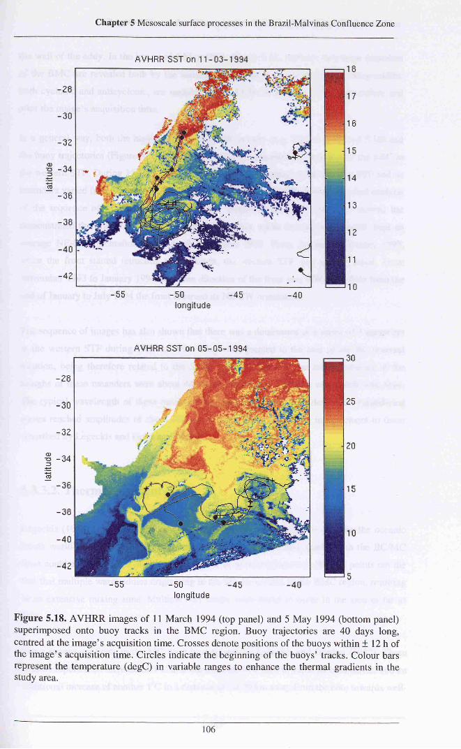
Chapter 5 Mesoscale surface processes in the Brazil-Malvinas Confluence Zone
AVHRR SSTon 11-03-1994
-50 -45
longitude-40
AVHRR SST on 05-05-1994
-42
-55 50 -45
longitude-40
Figure 5.18. AVHRR images of 11 March 1994 (top panel) and 5 May 1994 (bottom panel)superimposed onto buoy tracks in the BMC region. Buoy trajectories are 40 days long,centred at the image's acquisition time. Crosses denote positions of the buoys within 12 h ofthe image's acquisition time. Circles indicate the beginning of the buoys' tracks. Colour bars
represent the temperature (degC) in variable ranges to enhance the thermal gradients in the
study area.
106

Chapter 5 Mesoscale surface processes in the Brazil-Malvinas Confluence Zone
the wall of the eddy. In the image of 5 May 1994 (Figure 5.18, bottom), two large meanders
of the BMC are revealed both by the satellite image and by the buoy tracks. Three eddies,
both cyclonic and anticyclonic, are sampled by the LCDs in a period of 20 days before and
after the image's acquisition time.
In a general way, both the high-resolution AVHRR images (e.g. Figures 5.16 and 5.18) and
the buoy trajectories (Figure 4.3) have demonstrated the presence of meanders of the SAC in
the western STF. During 1993 to 1994, the predominant direction of the western STF and its
meanders varied from about 45 to 130 degrees (NE-SW to NW-SE). A more detailed analysisof the sequence of 81 high-resolution AVHRR images in the study area (not shown) has
demonstrated that the front and its associated meanders, while moving to the north, kept an
average NE-SW orientation from March to August 1993. From August to October 1993,
when the front started retracting to the south, the western STF was mainly zonal. From
November 1993 to January 1994 the mean direction of the front was NW-SE, while from the
end of January to July 1994 the front resumed its NE-SW orientation.
The sequence of images has also shown that there was a dominance of a series of 3 meanders
in the western STF during 1993 to 1994. They were located to the east of the BC reversal
location, being therefore related to the South Atlantic Current. The zonal positions of the
troughs of these meanders were about 44W and 48W, not changing very much with time.
The typical wavelength of these meanders was about 400 km. Well developed meandering
waves reached amplitudes of about 400 km as well. These values are in agreement to those
described by Legeckis and Gordon (1982).
5.3.3.2. Thermal gradients
Legeckis (1978) was one of the first authors to use satellite images to describe the oceanic
fronts worldwide. In his pioneering work, he showed that the SST gradients in the BC/MC
front could exceed values of 10C in a distance of several kilometres. He also points out the
fact that multiple warm eddies originating in the BC are present in the BMC region, resultingin an extensive mixing zone. Multiple SST fronts were found to occur in the area as far as
50S.
Cross-stream gradients in the MC were investigated by Legeckis and Gordon (1982). These
authors reported an increase of 1C in 2 km from the MC core towards its boundaries, and an
additional increase of another 1C in a distance of 10-20 km away from the core towards well-
107

Chapter 5 Mesoscale surface processes in the Brazil-Malvinas Confluence Zone
mixed waters. Extreme temperature changes across the MC/BC front were reported to reach
2.5C/km in the northern extreme of MC. In the eastern part of the BC reversal zone, Legekisand Gordon (1982) report maximum gradients of 3C in a distance of 2 km.
The SST gradients found for the MC/BC front in this work are in agreement with those found
by Legeckis (1978) and Legeckis and Gordon (1982), although the distances are somewhat
broader. As expected, the gradients across well detached eddies towards the neighbouringwaters tended to be smaller than those found across the western STF (MC/BC front). The
explanation for that lies in the process of coalescence of the individual eddies, where theytend to homogenise their temperatures with those from the surrounding waters over a periodof time. From this, knowing the magnitude of the SST gradients at the frontal system that
generates a particular eddy, and knowing the across-eddy temperature, the eddy's age could
possibly be inferred. At the moment we leave this possibility open for future work.
In order to illustrate the behaviour of the gradients found at the western STF and across eddies
formed in this area, Figures 5.20 to 5.25 present a series of transects taken from some of the
SST images considered representative of the BMC region. Because in the winter images the
MC core contributes to the development of the Brazilian Coastal Current, some of the
transects were made across the MC as well.
Figure 5.19 shows the SST image and two transects for 10 March 1993. In transect #1, a
gradient of 0.25C/km (6.1C in a distance of 24 km) was found between the MC core and
BC. The SST gradient of a warm core eddy in relation to surrounding (mixed) waters was of
1.6C in 24 km (0.06C/km). Gradients between the MC/BC mixed waters and a MC meander
were about 0.1C/km (2.3C in 20 km). In Figure 5.19, transect #2 crosses a cold core eddy at
a latitude of about 34S. This eddy has temperature characteristics of the mixed waters
between MC and BC, and is detached from the cold part of the front towards the BC waters.
The SST gradient between this eddy and the BC waters (to the west of it) was of 0.02C/km
(2.4C in 124 km). To the west of this eddy, a cold meander can be noticed in the processes of
forming another cold core eddy embedded in the BC.
Transect #1 in Figure 5.20 (27 April 1993) was taken across the BC/BCC front and across a
MC cold core eddy embedded in the warm part of the MC/BC front. BC/BCC gradient was
found to be 0.07C/km (4.2C in 56 km), while the gradient between the cold core eddy and
surrounding waters was of about 0.1C/km (8C in 88 km). Figure 5.20 also shows the coastal
waters off La Plata river and the MC core driving the BCC northwards. Transect #2 in this
figure indicated a gradient of 0.1 lC/km (4.6C in 40 km) between coastal waters and the MC
108

Chapter 5 Mesoscale surface processes in the Brazil-Malvinas Confluence Zone
core off the La Plata river, Argentina. The gradient between the MC core and BC in this
transect was 0.4C/km (15.8C in 40 km).
In the image of 3 August 1993 (Figure 5.21), the BC/BCC front is sampled in 2 transects. In
transect #1, taken at the Santa Marta Cape (~ 28S), the frontal gradient was 0.07C/km
(11.9C in 180 km). This gradient has the same order of magnitude as the one reported by
Zavialov et al. (1998) for the BC/BCC front in the area between 30S and 35S. To our
knowledge, this is the only reference explicit to the gradients of the BC/BCC front available
in the literature. It is worth mentioning, however, that the BC/BCC gradients tend to be higher
to the south owing to the proximity to the MC core. Transect #2 taken at about 35S, for
instance, indicated a gradient of 0.32C/km (6.4C in 20 km) for the BC/BCC front.
Transect #1 in the image of 8 November 1993 (Figure 5.22) illustrate the gradients between
the MC core and the typical MC eddies in relation to BC. In this case, the MC eddy was about
4C warmer than the MC core but, because of the across transect distances, the gradient
between the MC core and BC was smaller than between the MC eddy and BC. The gradients
were, respectively, 0.06C/km (8.7C in 156 km) and 0.2C/km (5.1C in 25 km).
Figure 5.23 shows the image of 27 January 1994 and a particular transect taken along the
MC/BC frontal axis. The transect #1 samples the MC core and two warm core eddies located
to the west of two MC meanders at about 40S. The gradient between the MC core and the
warm core eddy to the east of it was about 0.1C/km (6.7C in 60 km). Although the second
warm core eddy was about 3C warmer than the first one, the gradient between it and the MC
meander to its east was also close to 0.1C/km.
Another estimate of the gradients across the MC/BC frontal axis is illustrated in transect #1
of Figure 5.24 (5 May 1994). There, like in January 1994, the gradient between the MC core
and BC was 0.1C/km (11.6C in 116 km). Transect #2, in the BC/BCC front, indicated that
the SST gradient between these currents was about 0.03C/km (3C in 88 km).
109

Chapter 5 Mesoscale surface processes in the Brazil-Malvinas Confluence Zone
10-03-93, ironsect
240
220
I 200
2 180
I 1
^ 140
120
coastal waters-off Argentina
/
; / j
-V
p-MC
warm core
/ eddy/ cold core
Huu/jfVWA nil
mixed waters
core
MAi
clouds:/ i
mixed
> V\ /MC cold -
meander
100 2O0 300distance from the coast (km/4)
10-03-93, transect §2
coastal waters:off Uruguay
50 150 150 .200 250distonce from the coast (km/4)
Figure 5.19. AVHRR SST image of 10 March 1993 and the SST profile in 2 particulartransects across the image [SST=(Digital Number x 25.5)/255 + 5]. The square seen in the
image locates the cold core eddy present in transect #2.
27-04-93, transect
200
,-jr
150
100
BCC
clouds
'MC coldcore eddy
.
200 -
150
100
100 200 .300distance from the coast (km/4)
27-04-93, transect #2
coastal watersoff La Plata River
(BCC) ,BC
20 40 60,BO
. .
distance from the coast (km/4)100
Figure 5.20. AVHRR SST image of 27 April 1993 and the SST profile in 2 particulartransects across the image [SST=(Digital Number x 25.5)/255 + 5], The square seen in theimage locates the MC cold core eddy present in transect #1.
110

Chapter 5 Mesoscale surface processes in the Brazil-Malvinas Confluence Zone
160
^ 140
1 120c
ö 100
* 80
60
03-08-93.
r
\\\ BCC
irangect #1
V-V^VMfA, :
core / -
BC
-
-
20 40 60 SO 1QÖdistance from the coast (km/4)
03-08-93, Irangeci #2
20 40 60,
SO..
distance from the coast (km/4)100
Figure 5.21. AVHRR SST image of 3 August 1993 and the SST profile in 2 particulartransects across the image [SST=(Digital Number x 25.5)/255 + 5]. The square seen in theimage locates the BC/BCC front present in transect #2.
140
120
08-11-93. -trongect §^
50 100 150 200 21distance from the coast (km/4)
Figure 5.22. AVHRR SST image of 8 November 1993 and the SST profile in 1 particulartransect across the image [SST=(Digital Number x 25.5)/255 + 5]. The square seen in theimage locates the MC cold core eddy present in transect #1.
Ill

Chapter 5 Mesoscale surface processes in the Brazil-Malvinas Confluence Zone
27-01-94, transect250
200
150
100
BC warm
core eddyBC warm BC water
core eddy i '
distance300
Figure 5.23. AVHRR SST image of 27 January 1994 and the SST profile in 1 particulartransect across the image [SST=(Digital Number x 25.5)/255 + 5]. The square seen in theimage locates the BC warm core eddy present in transect #1.
I
t>
150
100
5D
0
05-05-94
-''"J!
MC core 1J 1 i
I
transect §
BC
J MC meander
coastal watersoff Argentina clouds
1
f:1 '
I :
MC,neander
1OO..
.200 300(km/4)
iQQdistance
05-05-94, transect #2
20 10 60 BO, .100
distance from the coast (km/4)
Figure 5.24. AVHRR SST image of 5 May 1994 and the SST profile in 2 particular transects
across the image [SST=(Digital Number x 25.5)/255 + 5]. The square seen in the imagelocates an instability wave at the BC/BCC front present in transect #2.
112

Chapter 5 Mesoscale surface processes in the Brazil-Malvinas Confluence Zone
5.4. Lagrangian measurements
5.4.1. Trajectories
The overall trajectories described by the LCDs are seen in Figure 4.3. Figure 5.25 shows the
overall trajectories only for the BC. In this figure, Brazil Current is seen flowing to the
southwest, meandering parallel to the South American coast. Meanders in the BC have the
same scale as those described for the western STF, e.g. 400 km. Visual comparison with the
bathymetry (Figure 1.1) suggests the tendency of the surface waters of BC to follow the
isobaths. In the vicinity of 31S this tendency is very well defined, where surface tracks
showed a major change in the direction of the BC flow from SW to W, responding to the
orientation of the isobaths of 200 m to 3000 m.
-55 -50
longitude
Figure 5.25. Trajectories described by the LCDs in the Brazil Current.
Very recently, the Brazilian government has set up a national plan (alas PNBoia, the Brazilian
National Buoy Programme) for the observation of surface currents using WOCE standard
Low Cost Drifters. Following the PNBoia, the INPE and the Brazilian petroleum company
113

Chapter 5 Mesoscale surface processes in the Brazil-Malvinas Confluence Zone
Petrobras had also set up another programme for the Lagrangian observation of surface
currents in the areas of interest for the petroleum industry in Brazil. The programme is known
as the SATBoia programme. Although the data set is not freely available yet, the updated
trajectories of the drifters already deployed by the PNBoia and SATBoia are available in the
world wide web at http://www.atsme.inpe.br/dsr/satboia. Figure 5.26 shows 2 maps where
PNBoia buoys number 32446 (launched on 14 April 1998) and 32458 (launched on 2 August1998) developed trajectories which followed the bathymetry at the Brazilian shelf break.
As the BC trajectories show in this work, the PNBoia drifters have also followed the majorchange in bathymetry at about 31S, just south of Santa Marta Cape. The comparison of the
PNBoia tracks with the ones presented by the LCDs used in this work also suggest that the
interaction of the BC with bathymetry at latitudes close to 31S is probably independent of
season and, therefore, of possible changes in the BC transport.
-36 -32 -2B -24- -SO
-44 -40 -Jß
s\
32457 Oep'ov
PNBOIA-Broril
Ir v
ment: 21 A^f. 98k
32458 Deplcyment: 21 -Aug.. 98 "/
j
4
/ftM
iAi j/f/A :
^0 Dee.9ß j
y \' 200 1000
^"-1 7 ; ;
-.. j.-. ; ; :
~k i
-Ad -40
Figure 5.26. Tracks of buoys 32446 (black line, left) and 32458 (blue line, right) in the BC
and SAC. Source: PNBoia home page (http://www.atsme.inpe.br/dsr/satboia).
Studying the BC path from 20S to 33S in 1985, Garfield (1990) verified that the regionsclose to Cabo Frio and south of Santa Marta Cape were the regions containing the highervariabilities of this current. To the south of Santa Marta Cape, Garfield (1990) suggests that
the change in the bathymetry would be enough to increase the variability in the front between
BC and coastal waters. Making an analogy with the interaction of the Gulf Stream with the
114

Chapter 5 Mesoscale surface processes in the Brazil-Malvinas Confluence Zone
Charleston bump, the author suggests that the interaction of boundary currents with
bathymetry is critical to their stability.
The adjustment of a stable flow drifting across the/-plane into a major change in bathymetryis explained by the conservation of potential vorticity. Owing to their design, the surface
floats used in this work and in the PNBoia program follow the waters at the average depth of
15 m. Changes in the relative vorticity of a flow are easier to be understood if the flow is
barotropic. However, for the eastern side of the BC/BCC front (along which our surface
LCDs drifted to the south) the isopicnal gradients are large. Below the BC, hydrographicaldata have demonstrated (e.g. Castro and Miranda, 1998) that the vertical gradients are also
considerable.
Preliminary investigations with the data of the LCDs in the Brazil Current at 31S (Souza and
Cabral, 1996) have indicated that the buoys used in this work did not significantly changetheir instantaneous velocities when changing direction because of the bathymetric effect.
However, the trajectories described by the buoys followed the//D (Coriolis parameter / depth)contours closely, which indicates the conservation of potential vorticity. The conception of a
numeric model to explore the surface Lagrangian behaviour of the BC along the shelf break
can provide improved understanding of the physical processes occurring at specific regions
along the BC path. The effects of specific conditions of transport, velocity and vertical
structure of the BC on its surface velocity field could be better understood with the help of a
numeric model. From the results presented here, it is evident that the vicinity of 31S is a
region that should be better studied.
Figure 5.27 presents the trajectories of the LCDs in the South Atlantic Current. SAC is seen
as a meandering zonal current flowing eastward in a band of latitudes that varied on average
from 29S to 40S. The size of meanders and eddies in this current varied from about 200 km
to 500 km. Eddies were much more present in the SAC than in the BC, being either cyclonicor anticyclonic. Remarkable eddy activity occurred at 37.5S, 52W.
Figueroa and Olson (1989) analysed the eddy diffusivity due to mesoscale motions in the
South Atlantic Ocean based upon FGGE and SOS (Southern Ocean Studies) drifter data sets.
Although still having a poor coverage of the boundary currents, the buoy measurements
improved the spatial coverage of velocity measurements in the South Atlantic, which was
considered to be very poorly observed. The buoy observations were almost entirely made in
the South Atlantic Current. SOS buoys were drogued at about 10 m, while FGGE buoys,when drogued, had several distinct drogue designs and depths. Trajectory maps shown by
115

Chapter 5 Mesoscale surface processes in the Brazil-Malvinas Confluence Zone
Figueroa and Olson (1989) were among the first Lagrangian descriptions of the SAC, and
indicate its general zonal orientation.
-50 -45
longitude-40 -35
Figure 5.27. Trajectories described by the LCDs in the South Atlantic Current.
Zambianchi and Griffa (1994) applied a stochastic model for particle motion to drifter data in
the South Atlantic Current. The authors used data from four SOS drifters deployed in 1984,
reporting that their buoys lay in two frontal regions between Brazil and Malvinas currents in
the open ocean. The first front, located at about 32S, was related to the Brazil Current waters,
while the second front (at 40S) corresponded, according to the authors, to the northern edgeof MC. The SAC, as derived from the Zambianchi and Griffa (1994) descriptions, had a
northeastern direction and was characterised by strong meanders of about 400 km in
wavelength and 200 km in amplitude. The meanders sizes described by Zambianchi and
Griffa (1994) are compatible with those measured by the LCDs used in this work, being also
in agreement with the description made by Legekis and Gordon (1982).
116

Chapter 5 Mesoscale surface processes in the Brazil-Malvinas Confluence Zone
5.4.2. Buoy time series
Figure 5.28 shows the time series of longitude, latitude and temperature measured by the
buoys in the Brazil Current during the time of this study. The BC was sampled by the buoysin four time periods during 1993 and 1994. The first period represents the Austral autumn
1993, the second represents the spring 1993, the third is the summer 1993, and the last is the
autumn 1994. The variations of longitude and latitude with time were similar all over the
period of study, with the buoys flowing from east to west and from north to south. A visual
inspection of the longitude and latitude time series shows periods of oscillation rangingbetween 12-20 days in the majority of the individual buoy series. Small period oscillations of
about 2 days were also present in the spring 1993 series.
-45
-5550 100 150 200 250 300 350 400 450
-30 -
-35 -
50 100 150 200 250 300 350 400 450
50 100 150 200 250 300 350 400 450
Julian day
Figure 5.28. Time series of longitude, latitude and temperature for the Brazil Current (colours
are in accordance with Figure 5.25).
The BC temperature time series suggests that temperatures of about 26C occur in the vicinityof 30S, 48W during the autumn and summer. These temperatures dropped to about 23C in a
range of latitudes from 31S to 37S and longitudes from 50W to 54W. During the spring
temperatures ranged from about 17C to 21C. From circa Julian day 270 to Julian day 300
117

Chapter 5 Mesoscale surface processes in the Brazil-Malvinas Confluence Zone
the temperatures increased approximately from 17C to 20C at a rate of about O.TC/day.Since the buoy launched in the BC during the spring 1993 drifted southward to a region where
cooler waters are expected to occur, the warming of BC waters to the south is likely to be
happening due to the seasonal heating.
Figure 5.29 shows the time series for the South Atlantic Current. This current is seen as a
zonal current, as only the longitude time series presents a considerable trend with respect to
time. Regardless of the season, the latitude time series are seen oscillating parallel to the time
axis, about an average position. This average however varies from one buoy to another
depending on the latitude of the buoy penetration into the SAC after exiting the BC. It can
also be said that regardless of the latitude of maximum penetration of the BC (which varies
seasonally), the SAC flows from this point zonally in a system of currents parallel with one
another.
-30
0
600
600
100 00 300
Julian clay400 500 600
Figure 5.29. Time series of longitude, latitude and temperature for the South Atlantic Current
(colours are in accordance with Figure 5.27).
118

Chapter 5 Mesoscale surface processes in the Brazil-Malvinas Confluence Zone
Temperature measurements made by buoy 3182 in the SAC also show a seasonal oscillation.
The semiannual cycle is obvious in the longer temperature time series of buoy 3182, where
temperature decreases from about 25C on Julian day 100 to 20C on Julian day 280. This
represents a rate of cooling of about 0.03C/day from late autumn to early spring. Oscillatorypeaks noticed in the longitude and latitudinal time series are related to eddy activity in the
current. In general, there are no peaks or troughs in the temperature time series associated
with the eddies. That is because the buoys were generally sampling the external walls of the
eddies, which are formed from instabilities of the mean flow in with the buoys were
previously embedded. In this case, the temperature measurements of the buoys at the wall of
an eddy remained the same as the previous measurements made by the buoys along the front
that generates the eddy.
5.4.3. Velocity, kinetic energy and temperature statistics
Table 5.3 shows the buoy-derived statistics obtained for BC and SAC in terms of its
velocities, kinetic energies and temperatures during the time of this study. This table and other
data presented here were published in a preliminary form in Souza and Robinson (1998).Surface (15 m) speeds in the BC were found to range between 12.2 cm/s to 53.6 cm/s in the
SW direction (37.4 cm/s in average towards 215.7), while SAC exhibited velocities from 4.2
cm/s to 16.6 cm/s to the east (9.7 cm/s on average towards 94.7). Eddy kinetic energies were
equal to 1294 cm2/s2 in the BC and 3268 cm2/s2 in the SAC. The temperature averages for
SAC were more than 4C cooler than that for BC, showing the influence of subantarctic
waters (SAW) in this current.
Schäfer and Krauss (1995) presented statistics for the major ocean currents in the
Southwestern Atlantic and in the ACC. They deployed more than 130 satellite-tracked
drifting buoys in the South Atlantic between 1990 and 1993, the majority of them drogued at
100 m depth. The BC mean velocity was found to be weak between 7S and 20S (4 cm/s),
increasing to 40 cm/s in the vicinity of the BMC region. The BMC region presented large
variability, with zonal and meridional r.m.s. currents of about 40 cm/s. In agreement with this
work, SAC was found to be almost zonal, presenting a mean velocity of 12 cm/s. BC shows
typical Eddy Kinetic Energy (EKE) varying between 200-400 cm2/s2. EKE values in the BMC
region reach 1600 cm2/s2, decreasing again in the SAC further east.
Piola et al. (1987), Stevenson and Souza (1994) and Stevenson (1996) also presented EKE
values for the BC derived from drifting buoy data. While Piola et al. (1987) worked with
119

Chapter 5 Mesoscale surface processes in the Brazil-Malvinas Confluence Zone
FGGE buoys, the last authors used the COROAS drifters. As in this work, EKE dominated
the BC flow in both cases, but Stevenson (1996) found these values to range between 13322; 2cm7sz and 4207 cm7s\ while Piola et al. (1987) found 500 cm7s
.
Table 5.3. BC and SAC velocity, kinetic energy and temperature statistics
(a) Brazil Current
buoy
317931813182
3185
3187
3188
3189
3190
31913192
mean
std.dev.
buoy
3182
3185
3187
3189
3190
31913192
mean
std.dev.
velocityspeed(cm/s)12.253.634.012.847.436.731.649.246.350.3
37.415.0
direction
(degrees)252.0212.1
181.7
237.1
214.4212.1
205.3
212.7
214.4
215.3
215.718.5
velocityspeed(cm/s)4.2
6.716.616.34.27.112.5
9.75.4
direction
(degrees)123.0
112.6
74.6
69.6111.2
88.1
83.5
94.7
20.8
MKE
(cmW)75143657782
112167449912091072
1265
801490
(b) South
MKE
(cmW)9
23
138132925
78
5957
kineticEKE
(cmW)10803576371901
899705100915302132743
1294937
Atlantic
energyTKE
(cm2/s2)11555012
948
983
2021
1379
1508
2739
3204
2008
20971266
Current
kinetic energyEKE
(cm2/s2)17692509341357692312
38763225
32681315
TKE
(cm2li)17782532355159012321
39013304
3327
1357
%EKE/
TKE
93.571.339.191.644.5
51.166.955.8
66.537.0
61.720.0
%EKE/TKE
99.599.196.197.899.699.397.6
98.41.3
temperaturemean
CQ24.1724.99
26.2719.1723.52
24.52
23.85
23.9724.56
24.00
23.901.83
std.dev
CQ0.960.730.130.820.760.430.720.86
0.660.99
0.710.26
temperaturemean
CQ22.5621.6917.66
18.6119.0818.75
18.61
19.57
1.82
std.dev.
CQ1.611.211.321.60
3.192.51
2.13
1.940.71
The Mean Kinetic Energy (MKE) in the BC was estimated to vary between 114-171 cm2/s2 byStevenson and Souza (1994), values in good agreement with 200 cm2/s2 found earlier by Piola
et al. (1987), but about 4 times lower than the average BC MKE presented here. Differences
between BC speeds measured by all these authors led to differences in MKE estimates. The
data used here represent the southernmost part of the BC flow, which is believed to have its
transport increased southwards (Garfield, 1990). Following the results obtained by Schäfer
and Krauss (1995), BC velocity can also increase southwards, which explains why MKE
values estimated here are higher than previous estimates.
120

Chapter 5 Mesoscale surface processes in the Brazil-Malvinas Confluence Zone
5.4.4. BC and SAC energy spectra
Figures 5.30 to 5.39 present the FFT spectra of the LCDs' temperature and instantaneous
(zonal and meridional) velocities time series for the BC. The FFT spectra of the LCD's time
series for the SAC are seen in Figures 5.40 to 5.46. The overall peaks found in the time series
of all drifters are presented, for simplicity, in Table 5.4. In the BC, peaks significant to the 95
% confidence interval were found to dominate the various spectra at 25.8 days (when the
series were long enough), 12.8 days, 8.6 days, and around 6.5 days and 3.5 days. Other
shorter period peaks were also found. Peaks at periods longer than 25.8 days were found in
the SAC time series, as the series were longer than the BC ones. In the SAC, for instance, the
time series generally presented dominant peaks of energy at 103.1 days and in the range from
22 to 30 days. Other peaks at around 41 days, 34 days, 11-13 days and shorter were abundant.
Because buoy 3182 was the longest series, is was possible to find a semiannual period at
204.1 days (6.7 months), with a possible second harmonic centred at about 103 days.
The relative importance of the semiannual peak for the South Atlantic has been discussed
early on in Section 5.2.2 of this thesis. According to Vivier and Provost (1999a), the
domination of the MC transport estimates by a semiannual cycle is compatible to the idea of a
remote forcing of this current. The finding of a semiannual peak in the SAC indicates that this
current, at the BMC region, is also responding to the large scale driven mechanisms occurringelsewhere in the South Atlantic. In addition, the period found here for the semiannual peak
(6.7 months) is also very similar to the one obtained before in this thesis when analysing the
seasonally averaged MCSST anomalies PC3 (Table 5.1).
Garzoli and Simionato (1990) utilised the same set of inverted echo sounders as Garzoli and
Garraffo (1989) in order to account for the high-frequency oscillations present at the BMC
front. These echo sounders were in a group of three, being deployed at about 37.5S, 52.5W.
Mainly due to the length of the echo sounders records, the oscillations were investigated in
the periods ranging from 55 days to 2 days. The physical parameters investigated were the
dynamic height, the distance of the instruments to the front and the wind stress at the surface,
which was inferred from the water column ambient noise.
For a band of period centred at 37.4 days, Garzoli and Simionato (1990) found a westward
propagating wave with amplitudes increasing linearly to the east (150 km to 258 km) and
phase speeds of 4.6 cm/s to 8 cm/s. The wave was proved neither to be a baroclinic Rossby
wave nor forced by the wind, but related to the movement of the BC/MC front. At the period
121

Chapter 5 Mesoscale surface processes in the Brazil-Malvinas Confluence Zone
of 29.1 days, another wave similar to that previously described was also found by Garzoli and
Simionato (1990). This wave had amplitudes of 250 km but propagated eastward, having the
same characteristics as the topographic Rossby waves present in the Gulf Stream. The forcingmechanism driving this oscillation is supposed to be the meandering of the Brazil Current at
the convergence zone.
Table 5.4. Period of the major energy peaks for the buoys' temperatureand instantaneous velocity time series in the BC and SAC
(dominant periods underlined)
(a) Brazil Current
buoy
3179
3181
3182
3185
3187
31883189
31903191
3192
Buoy
3182
3185
3187
3189
3190
3191
3192
temperature(days)
25.864
1.625.812.8
12.8; 6.4; 3.2; 1.612.8; 3.2; 1.4; 1.0
12.812.8
12.8; 5.1; 2.8
(b) South
temperature(days)
204.1; 41.0; 27.4; 17.1;10.5
103.1; 26.0; 18.9; 9.8;7.0
51.3; 12.8; 54; 3.3
103.1:224
103.1; 22.9; 11.7
103.1
103.1; 18.7
zonal instantaneous
velocity (days)
17.1; 5.7; 2.7; 1.8641.6
25.8; 5.7; 3.4
8.6; 3.3; 1.5
8.6; 1.2
12.8; 4.3
12.8; 2.9
6.5; 2.3; 1.2
8.6; 3.9; 14; 1.0
Atlantic Current
zonal instantaneous
velocity (days)
204.1; 41.5; 25.4;14.3; 10.7; 6.5; 5.8;
4.5; 3.6
103.1; 41.5; 22.4;12.9; 10.9; 7.3; 4.0
51.3; 17.1; 8.6; 6.0;3.8; 2.3; 1.7
103.1; 244; 17.0;12.6; 8.4; 6.1
50.2; 22.9; 13.4; 7.9;4.3
41.5; 26.0; 16.3; 10.9;6.3; 3.8; 3.0; 2.1
34.2; 12.9; 7.6; 5.4;3.5; 2.6; 2.0; 1.6
meridionalinstantaneous
velocity (days)12.8; 6.5; 2.7; 2.1
64
1.6
12.8; 3.7
12.8
12.8; 1.5
12.8; 4.3
8.6
12.8; 1.4
12.8; 2.9
meridionalinstantaneous
velocity (days)204.1; 71.9; 27.1; 17.4;13.7; 7.6; 5.5; 4.5; 3.0;
2.2; 1.8
34.2; 20.2; 9.0; 6.3; 3.5
25.4; 8.6; 64; 3.9; 2.6;2.1
29.5; 11.4; 6.8; 5.4;4.3; 3.1; 2.7; 1.8; 1.569.0; 22.9; 12.1; 4.7
22.9; 13.7; 9.4; 4.2;2.9; 2.2; 1.9
22.9; 10.9; 4.2; 3.1
122

Chapter 5 Mesoscale surface processes in the Brazil-Malvinas Confluence Zone
Higher frequency peaks of 2 days to 10 days were found by Garzoli and Simionato (1990) to
be not only forced by the wind stress (which gives the oscillation a seasonal variance in
energy), but also by the particular characteristics of the confluence: meandering, seasonal
displacement of the front, sea bottom topography (mainly the sharp slope) and changes in the
front's vertical structure which lead to baroclinic instabilities.
Comparing the oscillations found by Garzoli and Simionato (1990) with the ones found in this
work for the BC and SAC, it can be noticed that some of the peaks are very close in period,
suggesting that the driving mechanisms proposed by Garzoli and Simionato (1990) are
probably forcing some of the oscillations measured by the LCDs at 15 m depth. For instance,the peaks centred at about 22-30 days are close to the 29.1 days oscillation retrieved from the
echo sounders records.
The peaks close to 41 days and 34 days found for the SAC in the LCDs' measurements are
close to the 37.4 days oscillation reported by Garzoli and Simionato (1990). They can be
indicating the movement of the MC/BC front. Peaks close to 70 days found for the SAC are
very close to the bi-monthly incursions of the BC in the convergence suggested by Legeckisand Gordon (1982).
Some of the energy peaks of 10 days or less found in this work can also have their origins in
the same forcing mechanisms described by Garzoli and Simionato (1990). Owing to the lack
of other data taken in situ like wind data, for example, we can not link directly peaks of
energy in the buoy time series to their exact forcing mechanisms.
In agreement with Garzoli and Simionato (1990), the correlation between wind data and
oceanic oscillations in the Southwestern Atlantic Ocean was also reported by Stech and
Lorenzzetti (1992). Working in the South Brazil Bight (SBB), a region just north of the BMC
region, these authors have reported that the wind spectra has dominant peaks at 11 days and
6.5 days. Analysing sea level records at Paranagua, Brazil (~25.8S, 48.5W), Stech and
Lorenzzetti (1992) found a strong 7 days oscillation in the time series. With the wind data
showing a similar energy peak, Stech and Lorenzzetti (1992) concluded that the passage of
atmospheric systems is one of the major forcing mechanisms of the sea level in the SBB in
wintertime. Considering that the variations in the currents' direction and speed caused by the
passage of atmospheric fronts are more likely to be noticed at the surface layers of the sea,
above the Ekman layer, these oscillations are likely to be recorded in drifting buoys tracks.
Therefore, it can be assumed that the atmospheric forcing is the more likely cause of the
current oscillations at periods close to a week present in the buoy time series analysed here.
123

Chapter 5 Mesoscale surface processes in the Brazil-Malvinas Confluence Zone
BC, LCD#3179: temperature
4500
4000
3500
3000
I 2500
g 2000 -
-a
a 1500
f=
1000
500
oL10""
10*
10"' 10"frequency (cpd)
BC, LCD#3179: inst. zonal velocity
10
A
10"1 10frequency (cpd)
10
9000
ctnnnoUUU
7000
Ä60001^5000
density[
S3000QJc
2000
1000
n
BC, LCD#3179 inst meridional velocity
/ \ \ \
ij
-
-
!
;
_^^ /\
10"' 10frequency (cpd)
10
Figure 5.30. Energy preserving spectra of the LCD no. 3179's temperature (upper panel),instantaneous zonal velocity (middle panel) and instantaneous meridional velocity (lowerpanel) time series in the Brazil Current. The dashed lines represent the 95 % confidenceinterval.
124

Chapter 5 Mesoscale surface processes in the Brazil-Malvinas Confluence Zone
BC, LCD#3181: temperature
1200
10"frequency (cpd)
BC, LCD#3181: inst. zonal velocity
10'
10frequency (cpd)
BC, LCD#3181 inst meridional velocity
10
10"frequency (cpd)
Figure 5.31. Energy preserving spectra of the LCD no. 3181's temperature (upper panel),instantaneous zonal velocity (middle panel) and instantaneous meridional velocity (lowerpanel) time series in the Brazil Current. The dashed lines represent the 95 % confidenceinterval.
125

Chapter 5 Mesoscale surface processes in the Brazil-Malvinas Confluence Zone
x10" BC. LCD#3182: temperature
10Dfrequency (cpd)
BC, LCD#3182: inst. zonal velocity
10'
10"frequency (cpd)
BC, LCD#3182: inst. meridional velocity
10'
10frequency (cpd)
Figure 5.32. Energy preserving spectra of the LCD no. 3182's temperature (upper panel),instantaneous zonal velocity (middle panel) and instantaneous meridional velocity (lowerpanel) time series in the Brazil Current. The dashed lines represent the 95 % confidenceinterval.
126

Chapter 5 Mesoscale surface processes in the Brazil-Malvinas Confluence Zone
BC, LCD#3185: temperature
10*
14000
12000
7 10000
4000
2000
10
10
frequency (cpd)
BC, LCD#3185: inst. zonal velocity
10
10
frequency (cpd)
BC, LCD#3185: inst. meridional velocity
-
10" 10"frequency (cpd)
10'
Figure 5.33. Energy preserving spectra of the LCD no. 3185's temperature (upper panel),instantaneous zonal velocity (middle panel) and instantaneous meridional velocity (lowerpanel) time series in the Brazil Current. The dashed lines represent the 95 % confidenceinterval.
127

Chapter 5 Mesoscale surface processes in the Brazil-Malvinas Confluence Zone
BC, LCD#3187: temperature
2500
2000
1500
< 1000
500
10*
x104
10' 10"frequency (cpd)
BC, LCD#31B7: inst. zonal velocity
10'frequency (cpd)
BC, LCD#31B7: inst. meridional velocity
frequency (cpd)
10
10
10
Figure 5.34. Energy preserving spectra of the LCD no. 3187's temperature (upper panel),instantaneous zonal velocity (middle panel) and instantaneous meridional velocity (lowerpanel) time series in the Brazil Current. The dashed lines represent the 95 % confidenceinterval.
128

Chapter 5 Mesoscale surface processes in the Brazil-Malvinas Confluence Zone
BC, I_CD#3188: temperature
7000
6000
5000
E 4000
3000
2000
1000 -
9000
10
10"' 10"frequency (cpd)
BC, LCD#31B8: inst. zonal velocity
10'
10" 10"frequency (cpd)
BC, LCD#3188: inst. meridional velocity
Iff1 10frequency (cpd)
10'
Figure 5.35. Energy preserving spectra of the LCD no. 3188's temperature (upper panel),instantaneous zonal velocity (middle panel) and instantaneous meridional velocity (lowerpanel) time series in the Brazil Current. The dashed lines represent the 95 % confidenceinterval.
129

Chapter 5 Mesoscale surface processes in the Brazil-Malvinas Confluence Zone
BC, LCD#3189: temperature
15000
,10000
S 5000 -
10" 10"frequency (cpd)
BC, LCD#31B9: inst. zonal velocity
10-1 10frequency (cpd)
BC, LCD#3189 inst meridional velocity
10'
10' 10" 10
frequency (cpd)
Figure 5.36. Energy preserving spectra of the LCD no. 3189's temperature (upper panel),instantaneous zonal velocity (middle panel) and instantaneous meridional velocity (lowerpanel) time series in the Brazil Current. The dashed lines represent the 95 % confidenceinterval.
130

Chapter 5 Mesoscale surface processes in the Brazil-Malvinas Confluence Zone
BC, LCD#3190: temperature
8000
Itf1 10frequency (cpd)
BC, LCD#3190: inst. zonal velocity
10'
10
frequency (cpd)
BC, LCD#3190 inst meridional velocity
10'
frequency (cpd)
Figure 5.37. Energy preserving spectra of the LCD no. 319O's temperature (upper panel),instantaneous zonal velocity (middle panel) and instantaneous meridional velocity (lowerpanel) time series in the Brazil Current. The dashed lines represent the 95 % confidenceinterval.
131

Chapter 5 Mesoscale surface processes in the Brazil-Malvinas Confluence Zone
10"
BC, LCD*3191: temperature
10"' 10frequency (cpd)
BC, LCD#3191: inst. zonal velocity
10'
10-' 10frequency (cpd)
10
18
16
|14
^ 1
§0.8
|o.60.4
0.2
n
<104 BC, LCD#3191: inst meridional velocity
\
\
',
1
10" 10" 10'frequency (cpd)
Figure 5.38. Energy preserving spectra of the LCD no. 3191's temperature (upper panel),instantaneous zonal velocity (middle panel) and instantaneous meridional velocity (lowerpanel) time series in the Brazil Current. The dashed lines represent the 95 % confidenceinterval.
132

Chapter 5 Mesoscale surface processes in the Brazil-Malvinas Confluence Zone
BC, LCD#3192: temperature
6000
14000
12000
10000
8000
6000
4000
2000
10
101 10frequency (cpd)
BC, LCD#3192: inst. zonal velocity
10'
10-' 10frequency (cpd)
BC,LCD#3192 inst meridional velocity
10'
10' 10"frequency (cpd)
10'
Figure 5.39. Energy preserving spectra of the LCD no. 3192's temperature (upper panel),instantaneous zonal velocity (middle panel) and instantaneous meridional velocity (lowerpanel) time series in the Brazil Current. The dashed lines represent the 95 % confidenceinterval.
133

Chapter 5 Mesoscale surface processes in the Brazil-Malvinas Confluence Zone
1200
10"
16000
14000
_ 12000
% 10000
(J
~ 8000"55
'S 6000
aj
4000
2000
0
18000
16000
14000
ji 12000
"l 10000
4000
2000
010"
SAC, LCD#3182: temperature
10' 10-1frequency (cpd)
10
SAC, LCD#3182: inst. zonal velocity
V
r
. ..v '.n^kSvi^... ,
10" 10"' 10"frequency (cpd)
SAC, LCD#3182 inst meridional velocity
10
''S^Ä_..10'2 10"* 10
frequency (cpd)10'
Figure 5.40. Energy preserving spectra of the LCD no. 3182's temperature (upper panel),instantaneous zonal velocity (middle panel) and instantaneous meridional velocity (lowerpanel) time series in the South Atlantic Current. The dashed lines represent the 95 %confidence interval.
134

Chapter 5 Mesoscale surface processes in the Brazil-Malvinas Confluence Zone
SAC, LCD#3185: temperature
10
14000
12000
10000
E BOOO
2 6000
4000
2000 -
.
x 10
10' 10' 10"frequency (cpd)
SAC, LCD#31B5: inst. zonal velocity
10"frequency (cpd)
SAC,LCD#3185 inst meridional velocity
10"frequency (cpd)
10'
Figure 5.41. Energy preserving spectra of the LCD no. 3185's temperature (upper panel),instantaneous zonal velocity (middle panel) and instantaneous meridional velocity (lowerpanel) time series in the South Atlantic Current. The dashed lines represent the 95 %confidence interval.
135

Chapter 5 Mesoscale surface processes in the Brazil-Malvinas Confluence Zone
SAC, LCD* 3187: temperature
10
x 10'
10
x 10
10
10-' 10frequency (cpd)
SAC, LCD#31B7: inst. zonal velocity
10" 10"frequency (cpd)
SAC, LCD#3187: inst. meridional velocity
10-' 10frequency (cpd)
10
J.3
3
I 2.5
"e 2
i 1.5a>-o
>-.
enei
05
n
,, ,,,i , , , l
\
\
< ,' \
-
-
-
-
---^'V^Sr.ritf.i. L. I...!,..!.,
10'
10'
Figure 5.42. Energy preserving spectra of the LCD no. 3187's temperature (upper panel),instantaneous zonal velocity (middle panel) and instantaneous meridional velocity (lowerpanel) time series in the South Atlantic Current. The dashed lines represent the 95 %confidence interval.
136

Chapter 5 Mesoscale surface processes in the Brazil-Malvinas Confluence Zone
SAC, LCD#3189: temperature
10" 10"frequency (cpd)
SAC, LCD#3189: inst. meridional velocity
10
10- 10"frequency (cpd)
10
Figure 5.43. Energy preserving spectra of the LCD no. 3189's temperature (upper panel),instantaneous zonal velocity (middle panel) and instantaneous meridional velocity (lowerpanel) time series in the South Atlantic Current. The dashed lines represent the 95 %confidence interval.
137

Chapter 5 Mesoscale surface processes in the Brazil-Malvinas Confluence Zone
3000
10
14
12
10
10
4 -
2 -
10
x 1018
16
14
% 8c
>-. c?J O
ajcCD
4
2
010-
SAC, LCD#3190: temperature
10'
frequency (cpd)10 10
SAC, LCD#3190 inst zonal velocity
'.^".v.^Wcii^
10" 10"frequency (cpd)
10 10
SAC, LCDS3190: inst. meridional velocity
l>
10"2 10-' 10frequency (cpd)
10'
Figure 5.44. Energy preserving spectra of the LCD no. 319O's temperature (upper panel),instantaneous zonal velocity (middle panel) and instantaneous meridional velocity (lowerpanel) time series in the South Atlantic Current. The dashed lines represent the 95 %confidence interval.
138

Chapter 5 Mesoscale surface processes in the Brazil-Malvinas Confluence Zone
SAC, LCD*3191: temperature
10
x10*
x 10
10
10" 10"frequency (cpd)
10" 10
SAC, LCD*3191: inst. zonal velocity
10 10'frequency (cpd)
10" 10
SAC, LCD#3191: inst meridional velocity
10"frequency (cpd)
Figure 5.45. Energy preserving spectra of the LCD no. 3191's temperature (upper panel),instantaneous zonal velocity (middle panel) and instantaneous meridional velocity (lowerpanel) time series in the South Atlantic Current. The dashed lines represent the 95 %confidence interval.
139

Chapter 5 Mesoscale surface processes in the Brazil-Malvinas Confluence Zone
SAC, LCD#3192: temperature
10
x10
552-
10*
10' 10"frequency (cpd)
SAC, LCD#3192: inst. zonal velocity
10* 10"frequency (cpd)
10
SAC- LCD#3192: inst. meridional velocity
10"frequency (cpd)
10"
10'
A
to^Ä,10
10
Figure 5.46. Energy preserving spectra of the LCD no. 3192's temperature (upper panel),instantaneous zonal velocity (middle panel) and instantaneous meridional velocity (lowerpanel) time series in the South Atlantic Current. The dashed lines represent the 95 %confidence interval.
140

Chapter 5 Mesoscale surface processes in the Brazil-Malvinas Confluence Zone
5.5. Summary and final remarks
This chapter has studied some of the mesoscale surface processes occurring in the Brazil-
Malvinas Confluence zone during the period of March 1993 to July 1994. In order to support
our study, we have used a set of 168 MCSST images representing the South Atlantic as a
whole. This last data set was 14 year long, each image representing a monthly average for the
months from January 1982 to December 1995.
The processing of the MCSST data set provided 12 'climatological' monthly averages which
were used to describe the mean behaviour of the Subtropical Front in the South Atlantic, as
defined by the 20C isotherm at the surface. Utilising the original data and the
'climatological' data, monthly anomaly SSTs were also obtained for the particular months
between 1982 and 1995. They were subsequently grouped into their respective seasons. In
order to account for the periodicities of present in the SST fields in the Atlantic Ocean, both
'climatological' and anomaly SST images were submitted to Principal Component (PC)
analysis.
The climatological MCSST images have demonstrated that the Subtropical Front, as it was
measured by the 20C isotherm, reaches its northernmost position in September and retracts to
its southernmost position in February. The shape of the 20C isotherm in the BMC and
Southern Brazilian Continental Shelf (SBCS) indicates the penetration of cold waters in the
Brazilian shelf during the winter. It also shown that the meridionally orientated front between
tropical and coastal/subantarctic waters that happens in winter in the Southwestern Atlantic
Ocean is a continuation of the BMC or the Subtropical Front. This also supports the study
reported in Chapter 6 about the characteristics of the Brazilian Coastal Current.
The PC analysis performed in the climatological MCSST images indicated that the first four
components accounted for 99.92 % of the total variance of the data. The spatial amplitudes in
PCI were similar to the temporal mean of all images, while in PC2 the Subtropical gyre was
isolated from the rest of the South Atlantic. In this mode the so-called Atlantic Dipole is
noticed. The PCI, PC2 and PC3 eigenvectors indicate the annual cycle, which is dominant in
the South Atlantic. The semiannual cycle was present in PC3.
The first four PC modes of the seasonally averaged anomaly MCSST fields accounted for
78.04 % of the total variance in the data. The dominant peak for PCI and PC2 was centred at
5.37 years. PC3 and PC4 had their dominant periods centred at 10.7 years and 3 years,
141

Chapter 5 Mesoscale surface processes in the Brazil-Malvinas Confluence Zone
respectively. The annual cycle was found in PCI at 11.6 months. Intrannual oscillations were
centred in peaks ranging from 6.6 months to 10 months.
Analysis of the original monthly averaged MCSST images for the period between March
1993 and July 1994 revealed that this period of time was not particularly anomalous with
respect to the 'climatological' behaviour of the South Atlantic Ocean. That supports the
interpretation of the SST fields obtained for this period from the high-resolution AVHRR
images. The high-resolution images have demonstrated the presence of a series of mesoscale
features in the study area during the study period. In agreement with the MCSST
observations, the temporal sequence of high-resolution images also showed that a coastal
current develops at the SBCS during the wintertime, fed by waters from the BMC region.
The frontal surface activity in the study region could also be investigated by using the high-
resolution AVHRR images. Following the same procedure as for the MCSST images, the
20C isotherm was also used in these images to indicate the position of the frontal systems in
the study area. The BC/BCC front was particularly evident, lying parallel to the continental
shelf above the 100-200 m isobaths off Uruguay and Brazil. Being originated in the BMC
region, the front extends itself to the north of Santa Marta Cape (~28S), a position previously
thought to mark the limit in the SBCS for the penetration of waters with subantarctic
influence. For the first time in the literature it is also suggested that the BMC front can extend
itself to about 28S, further north than previously described.
Thermal gradients between the BC and the core of MC in the BMC region were found to be in
the order of 0.25C/km to 0.4C/km in horizontal scales of about 20 km to 40 km. The
gradients are smaller across the South Atlantic Current, between the warm and the cold part of
this current. The same is said for the gradients between eddies and their surrounding waters.
Gradients in the BC/BCC front were, as expected, smaller towards the north, owing to the
distance from the MC core. In a surface transect taken across the Santa Marta Cape in 3
August 1993, for example, the thermal gradient between BCC and BC was 0.07C/km.
The description of the thermal gradients of the BMC and SBCS regions is important in many
respects. Firstly, in previous literature, there were very few numeric descriptions of these
gradients and of their associated fronts, although they are very typical of the Southwestern
Atlantic and their strength facilitates their observation by satellite infrared sensors (Olson et
al., 1988; Podesta, 1997). Secondly, the frontal systems of the BMC and southern Brazil are
regions of concentration of biota, specifically fish (Castello et al., 1990, 1997). In these
regions the surface fronts are also a strong indicator of the process of water mixture occurring
142

Chapter 5 Mesoscale surface processes in the Brazil-Malvinas Confluence Zone
in the water column, as well as of the heat exchange. The monitoring of the surface waters off
Brazil started with project COROAS, when consistent satellite data was obtained for a periodof two years. Nevertheless, the continuous monitoring of the surface thermal fronts off Brazil
is still lacking for the period after 1994. Indeed, at the present time, the utilisation of satellite
images to monitor frontal systems for fisheries applications in Brazil still requires
development.
Buoy trajectories and time series of position and SST measured by the drifters were used here
to characterise the BC and the SAC during the period of this study. Buoy trajectories in the
BC and the SAC exhibited meanders and eddies which are consistent with previous
descriptions found in the literature for these two currents (e.g. Legeckis and Gordon, 1982).
The SAC was found to be about four times slower and to concentrate more EKE and TKE
(eddy and total kinetic energy) than the BC. In the BMC region, the BC average speed was
37.4 cm/s, while the SAC average speed was 9.7 cm/s. The BC mean temperature, as
measured by the buoys, was in average about 4C warmer than that from the SAC. BC flows
in the NE-SW direction, while SAC is mainly a zonal current in the study region.
Although the mean direction and meandering characteristics of BC and SAC are known to a
certain level, direct measurements of these currents are rare. Moreover, the comparisons made
in this thesis about their characteristic velocities, energies and temperatures are aspects that
have not been covered in known literature. In addition, the combination of satellite infrared
imagery and Lagrangian data for simultaneously studying the BC and SAC has not been fully
utilised until this research.
FFT spectra of the BC and SAC instantaneous velocity and temperature time series have
revealed energy peaks in periods shorter than those obtained for the South Atlantic when we
applied PC analysis on the MCSST data. The only time series long enough to show the
semiannual oscillation revealed in the PC analysis of the MCSST images was that of buoy
3182. There, the semiannual oscillation was centred at 6.7 months but only seen in the zonal
instantaneous velocity time series. The BC's most prominent peaks were centred at 25.8 days
(when the series were long enough), 12.8 days, 8.6 days, and around 6.5 days and 3.5 days. In
general, the SAC peaks were centred at 103.1 days, around 41 days and 34 days, 22-30 days
and at 11-13 days and shorter periods.
Some of the peaks found in the buoy time series are similar to others described in the
literature for the BMC region. According to Garzoli and Simionato (1990), the major forcing
mechanisms that generate the oscillations in the convergence region are many: meandering of
143

Chapter 5 Mesoscale surface processes in the Brazil-Malvinas Confluence Zone
the BC; meandering and seasonal displacement of the BMC; bottom topography; baroclinic
instabilities and wind stress. Changes in the MC or in the BC transports can also lead to
instabilities in the BMC. The balance between the distinct water masses including fresh water
coming from the La Plata River and Patos Lagoon outflows could also play an important role
in the local dynamics, but will probably affect only the western boundary currents, and not the
SAC. Differences in the oscillatory peaks present in BC and SAC can be related to locallydriven mechanisms acting in the BC and not in the SAC. This is an interesting subject for
further investigation.
144

CHAPTER 6
THE BRAZILIAN COASTAL CURRENT
6.1. Introduction
In this section we study the surface signature of the northeasterly coastal current which is
formed in the region of the BMC and was found to spread itself over the South Brazilian
Continental Shelf during the winter. High-resolution AVHRR imagery and Lagrangian data
collected in 1993 and 1994 are used here to describe the temperatures, velocity, energy and
oscillations present in this coastal current. These two data sets show that the current is not
only fed by cold waters from the BMC region, but also receives a contribution from the Brazil
Current at the surface by lateral mixing. By analysing the overall set of monthly averaged
MCSST images from 1982 to 1995, this section also demonstrates that the intrusion of cold
waters transported by the coastal current is a recurrent phenomenon occurring in the Brazilian
shelf in latitudes up to the vicinity of 24S during the months of June to October every year.
Given its consistency, this current is named here the Brazilian Coastal Current (BCC).
In a recent review paper, Castro and Miranda (1998) presented historical evidence of the
occurrence of a northeastly coastal current occurring in the region of the South Brazil Bight
(SBB). Although this current has been previously reported in the lower latitudes of the SBCS,
the lack of long term in situ data collection programmes for the SBCS region inhibited a
better characterisation and monitoring of this flow. It was only recently that consistent work
started being made towards a general description of this coastal current.
Satellite images have been available for Brazilian studies for many years, but it was only after
the establishment of the COROAS (Oceanic Circulation in the Western Region of the South
Atlantic) project in 1992 that a consistent routine for high-resolution AVHRR data collection
was set up in Brazil. Among COROAS objectives, satellite images were supposed to be used
1 This Chapter has been submitted to the Continental Shelf Research in the form of a paper entitled
'Lagrangian and satellite observations of the Brazilian Coastal Current', by Souza and Robinson.
145

Chapter 6 The Brazilian Coastal Current
together with simultaneous current measurements made by surface drifters for achieving a
better understanding of the BC behaviour off the Sao Paulo State coast, at about 23S.
Apart from the results concerning the BC, one of the new facts which came to light after the
experimental phase of COROAS is that low-salinity, cold waters formed in the BMC regionwere found to reach latitudes of about 24S, near Rio de Janeiro city during the winter of 1993
(Stevenson and Souza, 1994; Stevenson, 1996; Campos et al., 1996a; Campos et al., 1996b,
Silva Jr. et al, 1996).
From hydrographic surveys (e.g. Ciotti et al., 1995; Castro and Miranda, 1998), the consensus
in Brazilian oceanography was that cold waters coming from the south would reach maximum
limits of penetration of about 28S at Santa Marta Cape (Campos et al., 1996b) or perhaps27S at the Santa Catarina Island (Piccolo, 1998). Because of that and owing to the initiallylimited time series of satellite images collected through COROAS, the first results from this
project supposed that the intrusion of waters originating in the BMC to latitudes north of 28S
was an anomalous occurrence.
In a recent paper, for instance, Stevenson et al. (1998) used COROAS and other sources of
data to study the ecological aspects of the tropical Ilha Grande Bay (22S), off Rio de Janeiro
State, Brazil. These authors suggested that subantarctic organisms present there were, and are,
being carried along the SBCS by the cold waters originating in the south. These waters and
their associated alongshore movement were referred to by Stevenson et al. (1998) as the
northward extension of the Malvinas Current.
Stevenson et al. (1998), however, still considered that the entrance of subantartic biota to Ilha
Grande Bay happens in a sporadic way, leading to an interpretation that the coastal current
carrying the biota could also be sporadic. Stevenson et al. (1998) cited the passage of
meteorological fronts through the SBCS as an important, if not the principal, driving
mechanism for carrying waters with subantarctic origin to the north.
Ciotti et al. (1995) pointed out that the southern part of the Brazilian continental shelf is the
most important fishery area of the Brazilian coast. High phytoplankton biomass is related to
nutrients made available from the intrusion of SAW and CW in the platform. The possibility
of an extension of the most productive fishery area of the Brazilian shelf to the north of 28S
could surely have a significant economic impact in Brazil.
146

Chapter 6 The Brazilian Coastal Current
In this section, the behaviour of cold MC water in the BMC region and its extension in the
SBCS will be studied. In particular we wish to analyse further the character of the supposedanomalous behaviour, since it could be of considerable significance for the productivity and
the economic aspects of the area.
Lagrangian and high-resolution AVHRR data collected during COROAS are analysed in
detail to describe the temperatures, velocities, energies and oscillations present in the BCC.
Analysis of the BC/BCC thermal front, as seen in the AVHRR images, shows that surface
interactions between the poleward BC and the equatorward coastal current were present in the
form of small-scale (-20 km to ~50 km) shear instabilities during the 1993 and 1994 winters.
Monthly-averaged MCSST images of the South Atlantic Ocean are analysed for the period of
January 1982 to December 1995 to demonstrate that the intrusion of cold waters up to
latitudes near 24S is not an anomalous phenomenon, but rather a common process occurring
in the SBCS during every wintertime.
6.2. The BCC in 1993 and 1994
6.2.1. Trajectories and high-resolution imagery
The trajectories described by the LCDs in the BCC are seen in Figure 6.1. The tracks indicate
the Brazilian Coastal Current flowing northeastward parallel to the Brazilian coast on the
SBCS in water depths lower than 200 m. Eddy activity and meandering can also be noted
along all trajectories, but major activity is seen at about 25S, 46W, in the region near the
buoys' launching position. Although the buoys were launched together at the BC in February
1993, they entered the BCC in different positions and at different times (Table 4.2.b) after
April 1993. The time delay between the entrance of each single drifter in the BCC did not
result in much difference between the trajectories presented by the buoys.
Due to cloud cover, it was very difficult to match precisely the entrance times of each buoy
into the BCC from the BC with high-resolution AVHRR images. An image taken on 29 April
1993 (Figure 6.2), however, shows buoy 3179 entering BCC from BC, having been captured
by a small scale anticyclonic eddy, about 10 km wide, at the boundary between BC and BCC.
Another (warm core) eddy of the same scale as the one described in the trajectory can also be
spotted inside the core of BCC at about 31.25S, 50.25W in Figure 6.2.
147

Chapter 6 The Brazilian Coastal Current
-20
-25
13
-30
Rio de Janeiro.
BRAZIL
Santa Marta
-55 -50 -45
longitude-40
Figure 6.1. Trajectories described by the LCDs in the Brazilian Coastal Current.
The AVHRR images show that the frontal line separating BC from BCC is very distinct due
to the strong thermal gradients between the waters transported by these currents. Figures 6.3
and 6.4 show examples of these images where the temperature scale was adapted to enhance
the BC/BCC front. Lateral mixing is suggested by the presence of shear instabilities caused
by the two currents flowing in opposite directions. As noted in Figure 6.3, these instabilities
occur all along the front line between BC and BCC, and suggest that BC can feed BCC at the
surface by the detachment of warm core eddies. BCC also ejects cold core rings into BC.
Figure 6.4 represents a one-day sequence illustrating the development of a mushroom-like
structure in the BC in the vicinity of Santa Marta Cape at 28S. The process of surface
interleaving between BC and BCC is clear from this figure, and two warm core, cyclonic
rings about 50 km wide are in the process of formation in the BC at about 27.5S and 29S.
The eddies are apparently in the process to be expelled from the BC to the BCC. These
instability features are probably not in geostrophic balance (since geostrophically balanced
warm core rings have an anticyclonic gyre). Although relatively small, depending on the
periodicity and number of eddies formed they could account for much of the BC exchange of
heat and momentum with BCC along the front.
148

Chapter 6 The Brazilian Coastal Current
AVHRR SSTon 29-04-1993
-32.5 F"-.
-51 -50
longitude-49 -48
Figure 6.2. AVHRR image taken on 29 April 1993. BCC is represented by the cold waters
(green to blue) at the coast, while BC is represented by the warm waters offshore (yellow to
red). The image shows buoy 3179 entering BCC from BC after having been captured by a
small scale warm core eddy visible in the buoy's track (indicated by the arrow pointing to the
left). The possible equivalent of this eddy in the AVHRR image is indicated by the arrow
pointing to the right. The circle indicates the buoy's position 20 days before the images'acquisition time, the triangle indicates the buoy position within 12 h from the image'sacquisition time. The colour bar indicates temperature in degC).
Since lateral mixing and eddy formation happens throughout the BCC, it is supposed that the
position at which a particular buoy launched in the BC penetrates BCC through the front
depends randomly on the location where this particular buoy is caught by a warm core eddy
being formed. Both our Lagrangian and satellite observations have indicated that BC waters
can enter BCC all along the front between these two currents.
The observation of interleaving or instabilities along the BCC/BC front is also reported by
Lima et al. (1996). According to these authors, the entrainment of cold core eddies originatingin the coastal waters at the platform to the BC is an important mechanism for providing
nutrients from coastal or subantarctic origin to the oligotrophic Tropical Water (TW). Lima et
al. (1996) also report that cold core eddies in the BC can induce upwelling in the shelf break
and, together with the wind-driven circulation, produce a very distinct cross-shelf circulation
regime from winter to summertime.
149

Chapter 6 The Brazilian Coastal Current
AVHRR SSTon 05-06-1993
-54 -52 -50 -48
longitude-46
AVHRR SSTon 16-06-1993
-52 -50
longitude-48 -46
Figure 6.3. The BC/BCC front at the SBCS in 5 June 1993 (top) and 16 August 1993
(bottom). Buoys 3179 and 3180 tracks are seen in the image of 5 June 1993. Lateral mixing is
suggested by the presence of shear instabilities caused by the two currents flowing in oppositedirections. The arrows indicate the instability waves at the front. The circles indicate the
buoys' position 20 days before the images' acquisition time. The colour bars indicate
temperature in degC.
150

Chapter 6 The Brazilian Coastal Current
AVHRR SST on 19-07-1993
-49 -48 -47
longitude-46 -45
-27
-27.5
-28
a)
lati-29
-29.5
-30
-30.5
AVHRR SST on 20-07-1993
JEM'; ^
Jt
25
24
23
22
21
20
19
18
17
16
1549 -48 -47 -46
longitude-45
Figure 6.4. One-day sequence of AVHRR images taken in 19 July 1993 (top) and 20 July1993 (bottom). Buoy 3180 track is seen in both images. The sequence illustrates the
development of a mushroom-like structure in the BC in the vicinity of Santa Marta Cape at
28S (indicated by the arrows). The circle indicates the buoy's position 20 days before the
images' acquisition time. The colour bars indicate temperature in degC.
151

Chapter 6 The Brazilian Coastal Current
Early results from Lagrangian measurements made by the COROAS project in the SBCS
suggested that the BC recirculates in the platform (Stevenson and Souza, 1994; Stevenson,
1996). Following different paths along the SBCS, the period of recirculation computed from
the LCDs' trajectories varied from 115 to 161 days. These studies suggested the BC return
flow ends up becoming part of an MC extension inside the SBCS between 33S and 23S, but
have not proposed any explanation for that. Our data suggest that in fact the BC does not
recirculate inside the SBCS but exchanges mass and heat with BCC through turbulence alongits western limit.
Loder et al. (1998) reported that the majority of the ocean's western boundary currents flow
along the outer shelf or continental slope, providing a large source of momentum and water
mass properties to the coastal region due to their substantial associated volume transport.
They add that one of the best known forms of eddy activity affecting the western boundaryshelves is the transient warm core eddy generation from meanders of subtropical western
boundary currents. Other effects such as entrainment, vorticity waves, and on-shelf intrusions
or buffering water masses are quoted as also producing major influences from boundarycurrents in the adjacent continental shelves and coastal waters.
According to Loder et al. (1998), however, the western boundary currents' influence on
coastal waters decreases with increasing shelf width. In the SBCS, for instance, BC
wintertime influence in the shelf can be expected to be greater in the region of Santa Marta
Cape, where the shelf is only about 70 km wide in comparison to a typical width of 100 km to
150 km elsewhere.
The time series of latitude, longitude and temperature measured by the LCDs are seen in
Figure 6.5. Although entering the BCC on different dates, all time series show similarities in
their initial measurements when the buoys were flowing northeastwards. Each temperature
time series contains a quasi-constant cooling rate of about 0.12C per day when the buoyswere travelling northeastward in the BCC. Temperature measurements made by buoy 3179,
for example, decay from about 22C to 20C during the part of the trajectory when the buoywas flowing northeastward.
Comparing the SST measurements made by buoy 3179 with the SST image presented in
Figure 6.2, one can see that the warm core eddy shown there has a temperature of about 22C
and is surrounded by BCC waters at about 20C. This leads to an interpretation that the LCDs
entered the cooler BCC surrounded by warmer BC waters, probably inside small to mesoscale
152

Chapter 6 The Brazilian Coastal Current
eddies. Due to mixing, and consistent with the eddy dissipation, the temperatures measured in
the initial part of the LCD trajectories decay with time.
240 270 300
120 150 180 210 240 270 300
90 120 150 180 210 240Julian day in 1993
270 300
Figure 6.5. Time series of longitude, latitude and temperature for the Brazilian Coastal
Current (colours are in accordance with Figure 6.1).
6.2.2. Current velocity, kinetic energies and temperatures
The mean current speed and direction, kinetic energies and basic statistics for the time series
derived from the LCDs are presented in Table 6.1. Average surface (15 m depth) speed found
for the BCC was 11 cra/s (std. dev. = 6 cm/s) and the mean direction was 27 (std. dev. = 11).
From the trajectories, one can see that the BCC can reach the vicinity of 23S.
The BCC, in comparison to the BC, is relatively slow and flows in the opposite direction to
the latter. The BC velocity estimates and measurements, although still sparse, are much more
frequent than those of the BCC. Lagrangian estimates made using the COROAS dataset by
Stevenson and Souza (1994), Stevenson (1996) and in this thesis have demonstrated that the
BC speed varies from 15 cm/s to about 50 cm/s and that the current flows southwestwards.
153

Chapter 6 The Brazilian Coastal Current
As described before, direct measurements of the BCC are very sparse at the present. The few
measurements made, some of them not even paying attention to the speeds of the current,
were reported by Shaffer and Krauss (1995), Castro and Miranda (1998), Zavialov et al.
(1998) and Stevenson et al. (1998). Very recently, Zavialov and Möller (2000) have comparedthe model estimates described previously in Zavialov et al. (1998) with a time series of
current velocity obtained for a location at 3241'S, 5227'W. The current measurements were
made for a period between 4 March 1997 to 27 May 1997 by a conventional current meter
moored at 15 m depth above the 50 m isobath off the Patos Lagoon exit.
Table 6.1. BCC velocity, kinetic energy and temperature statistics
LCD
3178
31793180
averagestd.dev.
velocityspeed direction
(cmJs) (degrees)10
6
17
11
6
3515
31
2711
MKE
(cmW)5017
145
71
66
kinetic energyEKE TKE
(cmW) (cmW)2384771
2089
1748
859
24347882234
1819898
%EKE/TKE
97.9
97.8
93.5
96.4
2.5
Temperatureaverage std.dev.
CO (c)23.3419.8217.63
20.262.88
1.08
1.43
0.82
1.11
0.31
Zavialov and Möller (2000) found a very good agreement between model outputs and current
meter measurements for the current flowing northeastwards off the south of the SBCS region
and Uruguay. This current, named by the authors as the Rio Grande Current, was found to
have a seasonal average speed of up to 50 cm/s, but instantaneous values of up to 100 cm/s
were also registered in the current meter records.
Table 6.1 also indicates that the Mean Kinetic Energy (MKE) in the BCC varied from 17
cmVs2 to 145 cm2/s2, while the Eddy Kinetic Energy (EKE) varied from 771 to 2384 cm2/s2.
In Table 5.10 of this thesis we have presented MKE and EKE estimates for the BC and for the
South Atlantic Current. The mean MKE in the Brazil Current was 801 cm2/s2 and the mean
MKE in the South Atlantic Current was 59 cm2/s/2. Mean EKE estimates for the BC and the
SAC were 1294 cmV and 3268 cm2/s2. That represents, respectively, 61.7 % and 98.4 % of
the total kinetic energy present in the respective currents.
The result shown here for the BCC indicates that this current, as well as the SAC, contains
more than 95 % of its energy in small scale perturbations and eddy activity rather than in the
mean flow. Schaffer and Krauss (1995) have estimated that the EKE of the Malvinas Current
is about 500 cm2/s2. A maximum of 1600 cm2/s2, however, was found in the BMC region,
154

Chapter 6 The Brazilian Coastal Current
decreasing again farther east in the SAC. This indicates that the BCC and the SAC, both
extensions of the BC and the MC, respectively, seem to be less stable and more energetic than
their principal originators.
The temperature statistics for the BCC are also contained in Table 6.1. The mean value of
20.26C was found for this current. This mean is higher than that expected for the BCC as
seen from the satellite images, and can only be explained by the presence of warm water from
the BC being advected in the BCC, which is difficult to spot in the images. As discussed
before, the buoys were probably carried by these dissipating warm core eddies inside the BCC
and, therefore, the overall temperature measurements made by them probably did not
represent those typical of the neighbouring BCC waters.
6.2.3. BCC energy spectra
The FFT analysis of the buoys' time series in the BCC revealed the presence of energy peaks
significant at the 95 % confidence level at periods varying from 103.1 days to 1.5 days. The
FFT spectra for the temperature, instantaneous zonal velocity and instantaneous meridional
velocity time series obtained for the BCC are seen in Figures 6.6 to 6.8. Table 6.2 describes
the more energetic peaks.
A peak at 103.1 days was found in the temperature and instantaneous meridional velocitytime series of buoy 3179 (Figure 6.7). A peak at 70.4 days was present in the instantaneous
meridional velocity series of buoy 3179. Both time series of temperature of buoy 3178
(Figure 6.6) and instantaneous meridional velocity of buoy 3180 (Figure 6.8) presented a peak
at 51.3 days. Towards the lower periods, high energy peaks were most commonly found at
about 34-35 days, 29-30 days, 20-23 days, 10-13 days and 6-7 days. Many other peaks are
distributed at lower periods down to about 2 days.
The energy peaks found for the BCC are generally distinct from those found for the BC and
the SAC, which were described in Section 5.5.4 in this thesis. An exception to that occurs at
the periods close to 10-13 days which are mainly present in most of the BC time series but
also in some of the SAC and BCC series.
According to Castro and Miranda (1998), the current variability in the middle and inner South
Brazilian Bight shelf is dominated by subtidal and tidal oscillations. Large energy peaks,
155

Chapter 6 The Brazilian Coastal Current
10
.
x10
10
x10
BCC, LCD* 3178: temperature
frequency (cpd)
BCC, LCD#3178: inst. zonal velocity
10"' 10"frequency (cpd)
BCC, LCD*3178: inst. meridional velocity
10-' 10frequency (cpd)
10'
10'
10
Figure 6.6. Energy preserving spectra of the LCD no. 3178's temperature (upper panel),instantaneous zonal velocity (middle panel) and instantaneous meridional velocity (lowerpanel) time series in the Brazilian Coastal Current. The dashed lines represent the 95 %confidence interval.
156

Chapter 6 The Brazilian Coastal Current
10'
10
BCC, LCD#3179: temperature
10'frequency (cpd)
BCC, LCD#3179: inst. zonal velocity
10
10"* 10"' 10"frequency (cpd)
10
flnnnuUUU
7000
6000-aa.
'J'sooo
f 4000"v>
"^3000a>
2000
1000
n
BCC, LCD#3179 inst meridional velocity
ii
. . .^
^' A'"'
\\\
i! i
'i \\
.Hi '\,
--.'.. ~..., v^^.~
10"* 10" 10"frequency (cpd)
10
Figure 6.7. Energy preserving spectra of the LCD no. 3179's temperature (upper panel),instantaneous zonal velocity (middle panel) and instantaneous meridional velocity (lowerpanel) time series in the Brazilian Coastal Current. The dashed lines represent the 95 %confidence interval.
157

Chapter 6 The Brazilian Coastal Current
10*
x1Cf
10
x 10
10
BCC. LCD#31B0: temperature
10
frequency (cpd)
BCC, LCD#3180: inst. zonal velocity
10
10" 10"frequency (cpd)
BCC, LCD#31B0: inst. meridional velocity
10
10"' 10"frequency (cpd)
10'
Figure 6.8. Energy preserving spectra of the LCD no. 3180's temperature (upper panel),instantaneous zonal velocity (middle panel) and instantaneous meridional velocity (lowerpanel) time series in the Brazilian Coastal Current. The dashed lines represent the 95 %confidence interval.
158

Chapter 6 The Brazilian Coastal Current
however, are concentrated in the periods of 3-7 days and at 9-15 days, the same as the windand sea-level oscillations. These authors, for instance, report that the occurrence of the frontalsystems (which are driving the winds' intensity and direction) over the Southwestern AtlanticOcean between 20S and 34S has a time scale of 5-10 days between passages.
Table 6.2. Period of the major energy peaks for the buoys' temperature andinstantaneous velocity time series (dominant periods underlined):
Brazilian Coastal Current
buoy
3178
3179
3180
temperature(days)
51.3
103.1:28.9
34.5; 5.0
zonal instantaneous
velocity (days)
20.7: 11.5:5.8:4.5:3.3;2.3; 1.7
103.1:29.5:20.2; 12.1;9.2; 7.4; 5.9; 4.0
33.9; 10.4; 6.9; 3.6; 2.7
meridionalinstantaneous
velocity (days)12.6; 5.7; 4.6; 3.3; 1.7
70.4; 23.1; 12.1; 7.8;4.2; 3.2
51.3; 13.0; 6.5; 3.6;3.0; 2.1; 1.5
As reported in Chapter 5 of this thesis, peaks of 11 days and 6.5 days were found in wind data
of the SBB by Stech and Lorenzzetti (1992). Analysis of sea level data in the same regiondemonstrated the existence of a peak centred at 7 days, which Stech and Lorenzzetti (1992)
have associated with the atmospheric pressure systems crossing the SBB.
Stech and Lorenzzetti (1992) pointed out that the passage of low-pressure atmospheric
systems is one of the major forcing mechanisms present in the SBB during wintertime. The
cold atmospheric fronts occurring in the SBB were reported to have a displacement speed of
500 km/day in the southwest to northeast direction. This is the same direction as the BCC
current. Stevenson et al. (1998), studying the intrusion of cool waters in the SBCS, also
considered that the atmospheric forcing would drive the northeasterly currents in that region.
6.3. The BCC and BC extreme positions
The mean oscillation of the STF between 1982 and 1995, as seen from the MCSST monthly
climatological averages, was already discussed in Section 5.2.1. As pointed out before, the
western extreme of the STF indicates the BMC, and the two extreme vertices of the
characteristic 'Z' shape of the 20C isotherm in the BMC region indicate the location of the
maximum penetration of both the MC (and its extension, the BCC) and the BC. In this section
we analyse the overall set of 168 MCSST monthly averaged images taken from January 1982
159

Chapter 6 The Brazilian Coastal Current
to December 1995 to track the extreme positions reached by both the BCC and the BC duringthat period of time. As described in Section 4.2.3, the positions of maximum penetration for
both the BC and the BCC were treated in the form of a time series of longitude and latitude
per month from January 1982 to December 1995.
Because the extreme positions of MC or BCC and of BC were taken simultaneously from the
same isoline in each particular MCSST image, their time series are related to each other. Theywill be compared here. Considering that the BCC is an extension of the MC towards the coast
in the region of the SBCS, we will simply refer to the MC extreme positions as the BCC
extreme positions.
Figure 6.9 shows the extreme position time series for both the BCC and the BC. Peaks in the
time series are associated with the wintertime. The seasonal oscillation of the BCC and the
BC extremes is clearly seen at the western extreme of the STF in Figure 5.1. Since the
oscillation of the currents is parallel to the Brazilian coast, westward displacement is coupledwith southward movement, and eastward movement has its northward counterpart. The time
series of BC longitude extremes is noisier than the other series, and the zonal displacement of
this current is wider, as expected. The BC southernmost extremes are located in the origin of
the SAC, and its position is not restricted to the continental shelf.
The minimum and maximum latitudinal positions found for the BCC were 39.1S and 23.6S
occurring in February 1984 and August 1983 (Figure 6.10), respectively. The difference
between minimum and maximum latitude positions for the BCC is 15.5, which is about 1700
km. For the BC, on the other hand, the minimum and maximum latitudinal extremes were
43.8S and 28.3S in February 1984 and October 1987, respectively. The latitudinal difference
between the BC extremes was 15.5, by coincidence the same as found for the BCC.
Table 6.3 and Figure 6.11 show the basic statistics (mean and standard deviation) resultingfrom the BCC and the BC extreme position locations for each month from January 1982 to
December 1995. August was the month when in the mean both the BCC and the BC reached
their northernmost limits. The mean north extreme for the BCC was 25.2S (std.dev. = 1.6),
and for the BC 3O.3S (std.dev. = 1). For the southernmost extremes, the BCC presented a
mean latitude of 37.2S (std.dev. = 1), and BC of 42S (std.dev. = 1). Hence, the BCC was
found to oscillate an average 12 in latitude, which represents 1334 km. The BC, on the other
hand, was found to oscillate an average of about 11.7 in latitude or 1301 km.
160

Chapter 6 The Brazilian Coastal Current
BCC longitude extremes BCC latitude extremes
82 84 86 88 90 92 94 96
BC longitude extremes
82 84 86 88 90 92 94 96
BC latitude extremes
82 84 86 88 90 92 94 96
year
82 84 86 88 90 92 94 96
year
Figure 6.9. Extreme position time series for the BCC and BC.
lOS I
ririR
H 5C
v'
W 40
L.longitudelongitude
Figure 6.10. MCSST images for February 1984 and August 1983 indicating the minimum
(left) and maximum (right) latitudinal position of the BCC for the period of 1984 to 1995. The
black line represents the 20C isotherm.
Reid et al. (1977) report that the position in which the BC reverses its direction (interpreted
here as the BC southernmost extreme) is between 40S and 46S. These authors add that this
position is further south than the mean BMC oscillation region. Legeckis and Gordon (1982)
161

Chapter 6 The Brazilian Coastal Current
found the latitudes of 38S to 46S as the maximum limits for warm water related to the BC.
The southernmost extreme of the BC occurrence found in this work (42S 1 std. dev.) is in
agreement to those found by Reid et al. (1977) and Legeckis and Gordon (1982). As it was
not their objective, neither paper accounts for the northermost extreme of the MC (or its
extension) along the South American coast.
BCC longitude extremes BCC latitude extremes
123456 789101112
BC longitude extremes
1 23456789101112
BC latitude extremes
123456 789101112months
1 23 456789101112months
Figure 6.11. Statistics for the BCC and BC extreme positions per month.
Working with full-resolution AVHRR data collected between July 1984 to June 1987, Olson
et al. (1988) established the statistical characteristics of the separation region from the
continental shelf (position of crossing with the 1000 m isobath) for both the BC and the MC.
Considering the BC, these authors found that this current separates from the coast at the mean
latitude of 35.8S, with a standard deviation of 1.1. However, the total range of latitudes
where the BC separates from the coast (difference between maximum and minimum values)
was found to be 4.8. This value is less than half the value of 11.7 found here for the BC
162

Chapter 6 The Brazilian Coastal Current
oscillation. Causes for this disagreement are possibly related to the different methodologiesemployed to describe the BC extremes by Olson et al. (1988) and in this thesis.
Table 6.3. Statistics for the BCC and BC extreme positions over the year
month
Jan
Feb
Mar
AprMayJun
Jul
AugSepOctNov
Dec
lat. BCC CS)mean
36.8
37.236.834.1
32.4
29.426.525.2
25.8
29.1
31.834.6
std.dev.
0.91.0
0.6
0.5
0.62.8
2.3
1.61.81.71.11.3
long.mean
54.154.754.3
53.351.4
49.4
47.446.3
47.0
48.9
50.953.3
BCC CW)std.dev.
0.8
0.7
0.8
0.50.7
1.81.4
1.6
1.2
1.0
1.0
1.3
lat.
mean
41.342.0
42.0
40.4
36.734.2
32.130.330.531.9
34.538.3
BCfS)std.dev.
1.41.11.0
1.41.11.11.61.01.31.51.71.5
long.mean
52.151.951.851.049.849.747.346.246.447.749.849.9
BCCW)std.dev.
1.71.5
1.2
1.63.51.92.71.92.22.3
1.23.3
While Olson et al. (1988) described the position where the BC separated from the coast at the
1000 m isobath, in this thesis we located the position where the 20C isoline reached its
southernmost extreme in the BMC region. Besides this, the time series used in this work is far
more extensive than the one used by Olson et al. (1988), which was restricted to 1984 to
1987.
As noted in Figure 6.9, the years of 1985 and 1986 (both included in Olson's paper) are also
seen in the time series as years when the BCC and the BC had their wintertime northernmost
limits reduced by about 3 in latitude with respect to adjacent years. This leads to an
interpretation that 1985 and 1986 (as well as 1994 - note Figure 6.9) have had anomalouslymild winters, which reduced the penetration of the BCC. Explanations for that cannot rely on
the occurrence of El Nino, for instance, since this phenomenon did not occur either in 1985-
86 or in 1994. In the winters of 1985-86, the La Plata river also did not display any anomalous
outflow in relation to adjacent years (Raul Guerrero, personal communication).
In recent works, Sunye and Servain (1998) and Sunye (1999) investigated the effects of the
climatological variability of the ocean on the sardine Sardinella brasiliensis fisheries in the
region between Santa Marta Cape and Cabo Frio (~23S to 28S). Utilising historical
hydrographical data, Sunye (1999) determined the temperature fields for the South Brazil
Bight and studied the penetration of waters of subantarctic origin in the study region from
163

Chapter 6 The Brazilian Coastal Current
1982 until 1992. The author utilised the distribution of the 20C isotherm for the month of
August to conclude that the mean latitude of maximum penetration of cold waters in the SBB
is 24S during this month. This latitude is in agreement to the one found in this work (25.2S+ 1.6 std. dev.) and is an indication that the MCSST data set used here is reliable for use in
coastal regions for climatological purposes.
Sunye and Servain (1998) studied the landings of the sardine in three Brazilian states from the
south to the north of the SBB (Santa Catarina, Säo Paulo and Rio de Janeiro, respectively).The principal fishing harbours at these states are, respectively: Itajai (~27S), Santos (~24S)and Rio de Janeiro city (~23S). Total catches were computed per month for the periodbetween 1980 and 1990. The complementary percentage of the total catch of sardine per
month in Santa Catarina, Säo Paulo and Rio de Janeiro is seen in Figure 6.12.
Following Sunye and Servain (1998), Figure 6.12 indicates that the landings of sardine in Rio
de Janeiro, in the north of the SBB, are relatively low thoughout the year. They represent 20
% of the total Brazilian catches. Each of the other two states at time, on the other hand, can
alone account for up to 60 % of the total catches depending on the season of the year. In Säo
Paulo, for instance, the landings are high in winter (maximum in August) and low in summer
(minimum in February). The reverse is true in Santa Catarina state. Sunye and Servain (1998)
conclude that the sardine landings in the two Brazilian states to the south of the SBB are
affected by meteorological and oceanographic parameters. The major cause of the variations
in the oceanographic factors in the SBB is the penetration of the less saline (coastal or
subantarctic) waters in the Brazilian shelf.
By comparing Sunye and Servain's (1998) Figure 6.12 with Figure 6.11 it is very clear that
there is a coincidence between the latitudinal extreme positions of the BCC (Figure 6.11,
upper right panel) and the sardine catches in Säo Paulo and Santa Catarina. When BCC
northern limits are to the south of SBCS during the months of summer, the sardine catches are
higher in Santa Catarina. When BCC latitudinal extrema are displaced to the north in winter,
the catches of sardine are higher in Säo Paulo. The investigation of the relationship between
sardine catches and the position of the 20C isotherm (an indication of the BCC/BC front
northern extreme) measured by satellites in the SBCS can be a step forward towards the
predicability of the Sardinella braziliensis catches in Säo Paulo, considering that the fisheries
effort is also known.
164

Chapter 6 The Brazilian Coastal Current
JFMAMJ JASON D
70
SO
140
I 30
aoI
i
1
JFMAMJJASOND
I FMAMJ J ASONO
Figure 6.12. Total catch of sardine (Sardinella brasiliensis) in the SBB for the periodbetween 1980 and 1990. Panels ordered from bottom to top represent complementarypercentages of the total catch for three Brazilian States from south to north (Santa Catarina,Sao Paulo and Rio de Janeiro), respectively. Error bars represent 1 standard deviation.Fisheries of sardine is prohibited in January, hence there are no data available for that month.Source: Sunye and Servain (1998).
Figure 6.13 displays the BCC and the BC extreme positions along the South American coast
for the different seasons of the year (summer: December to February; autumn: March to May;winter: June to August; spring: September to November). It seems that the vicinity of 32S
marks the extremity of occurrence of the BCC during summer and autumn months. To the
north of 32S, the BCC only penetrates the SBCS during the winter or spring months. The
BCC extreme position, as seen by the distribution of the crosses in Figure 6.13, is continuous
along the SBCS and restricted to isobaths shallower than 200 m (not shown) in the inner
shelf, consistent with the trajectories described in this current by the LCDs in 1993 (Figure
165

Chapter 6 The Brazilian Coastal Current
6.1). The BC distribution for all seasons, on the other hand, is broader, not shelf-constrained
and resembles, as expected, the distribution of the frontal systems analysed for the study area
in Chapter 5 using high-resolution AVHRR data (Figures 5.17 and 5.18).
BCC(+) and BC(o) extremes by season
-60 -55 -50 -45
longitude-40
Figure 6.13. BCC and BC extreme positions per season in the SBCS.
6.4. Summary and final remarks
In this chapter, the Brazilian Coastal Current is described as a relatively slow but highly
energetic coastal current, flowing in the opposite direction to the Brazil Current. The current
occurs over the South Brazilian Continental Shelf during spring to wintertime, reaching its
maximum extreme at about 24S in August every (non-anomalous) year.
High-resolution satellite imagery and surface drifters have been used in conjunction to
demonstrate that warm core rings expelled from the BC enter the BCC and are advected
northeastward with this coastal current. MCSST data collected from 1982 to 1995 were used
to track the extreme positions for the BC and the BCC, and to demonstrate that the
penetration of the BCC on the SBCS to latitudes of about 24S is not anomalous but rather the
normal process occurring most years in the Brazilian continental shelf. One of the principal
166

Chapter 6 The Brazilian Coastal Current
mechanisms to drive the BCC penetration is believed to be related more to the large-scaleoscillation of the Subtropical Front in the open South Atlantic Ocean than to the local winds
at the Brazilian coast.
60W20"S-
55'W 50*W 45"W 40"W
45"S
Brazil Current
Ivinas Current
Brazilian Coastal Current
26'S - South Atlantic Curret!
3O'S
35"S
40"S
60*W 55"W 50"W 45"W 40'W
Figure 6.14. Schematic illustration of the surface currents in the SBCS and BMC regions.BCC occurs in wintertime as an extension of MC carrying coastal waters in latitudes lower
than 32S.
Using both the Lagrangian and the MCSST dataset presented here, Figure 6.14 presents a
schematic interpretation of the mean BCC and BC distributions through the year at the SBCS.
Although recent papers have dealt with the current distribution in the South and Southwestern
Atlantic (e.g. Peterson and Stramma, 1991; Piola and Rivas, 1997; Loder et al., 1998), all of
them fail to propose a satisfactory scheme for the BCC domain in the SBCS during the
winter. A simple, didactic scheme like the one seen in Figure 12, was never before proposedfor the Southern Brazilian continental shelf region, and can be used in future studies plannedfor that region.
167

Chapter 6 The Brazilian Coastal Current
Bearing in mind that SAW and CW transported by the BCC are much more productive than
the oligotrophic TW transported by the BC (Hubold, 1980; Castello et al., 1990; Ciotti et al.,
1995; Seeliger and Odebrecht, 1997; Nienchesky and Fillmann, 1997), the environmental and
economic aspects of the wintertime domination of the SBCS by waters with subantarctic and
coastal origin is of considerable significance and needs to be understood urgently. The
relation between the BCC and the sardine fisheries in the SBCS was explored to some extent
here, but the relation between this current and other fisheries stock in the Brazilian shelf oughtalso to be studied.
Remaining questions to be answered about the BCC behaviour concern its relation with the
discharge cycles in the La Plata river and Patos Lagoon, the local winds along the Brazilian
shelf and the oscillation of the STF. Although the STF oscillation in the South Atlantic Ocean
is supposed here to be one of the major forces governing the BCC intrusion further north in
the Brazilian platform, the local winds blowing from the south have a contribution which
needs to be better understood. The Ekman transport and the sea level elevation (which
depends on the continental outflow among other factors) are indicated by Zavialov et al.
(1998) to be the forcing mechanisms for the northbound currents occurring at the southern
part of the SBCS.
The complete understanding of the dynamical structure, variability, water mass composition,
spatial signature and other characteristics of the BCC can only be assessed through the
establishment of long-term direct measurements in the current. The study of the relations
between the development of the BCC and the processes occurring at the BMC region, as well
as connections with the large scale processes in the Atlantic or Pacific, should also be the
subjects of further research.
168

CHAPTER 7
EDDY OBSERVATIONS AND CHARACTERISATION
7.1. Introduction
In this section we investigate the characteristics of the eddies found in the Southwestern
Atlantic Ocean in 1993 and 1994 as they were measured by the combination of surface
drifters and high-resolution SST images. The investigation of these eddies is made accordingto their characteristic sizes (perimeters or diameters), rotational periods and velocities, Rossbynumbers and relation to the local internal Rossby radius of deformation.
In the Southwestern Atlantic Ocean, most of the eddy activity is related to the BMC region
(e.g. Legeckis and Gordon, 1982; Olson et al., 1988). Nevertheless, the characterisation of the
BMC eddies is generally restricted to their sizes and location. Given the relatively few in situ
data, most of the works have described these structures using only remote sensing images. To
our knowledge, very few references are available describing other eddy properties such as
their rotational periods or tangential velocities, for instance. These are important parameters
for describing the eddy field more realistically, and are studied in more detail in this thesis.
With respect to the South Brazilian Continental Shelf (SBCS), the situation is a little worse
than that of the BMC region. Some previous descriptions of the eddies in the Brazil Current
can be found in the works made by Garfield (1990) and Schmid et al. (1995), for example.
Unfortunately, these individual efforts fail to provide a general description of the eddies
across the SBCS and over long periods of time. Some eddy activity in the SBCS was also
described in the first results from the COROAS project (e.g. Lorenzzetti et al., 1994; Campos
et al., 1996a; Stech et al., 1996) and, very recently, in the first results of oceanographic
programmes conducted by INPE (e.g. Lorenzzetti and Kampel, 1998). The initial COROAS
papers, although using some of the same material as studied in this thesis, have generally
dealt with specific events, neither addressing the overall COROAS experimental phase nor
making any comparison to other eddies found in the Southwestern Atlantic Ocean, as will be
presented in this chapter.
169

Chapter 7 Eddy observations and characterisation
In our systematic study of the available data, small eddies, generally ignored when utilisingremote sensing techniques because of the difficulty in spotting them, have been found to be
present in both the AVHRR images and in the buoy trajectories. They were associated with
the three currents studied: the BC, the BCC and the SAC. These eddies were several times
smaller than the typical Rossby radius of deformation for the regions of the BMC and of the
BC/BCC front, indicating extremely turbulent fluxes or wind driven circulation where inertial
forces were much more important than the rotational forces.
Some of the eddies present in the BC/BCC front were similar to the shelfbreak eddies found
in the Middle Atlantic Bight off the United States east coast (e.g. Garvine et al, 1988).Inshore eddies present in the BCC, however, seem to be related to current reversals probablycaused by the passage of atmospheric fronts. To our knowledge, apart from references in
some COROAS papers to their presence in the buoy tracks (e.g. Stevenson, 1996), neither the
characteristics of the BCC eddies nor the possible driving mechanisms involved in their
generation at the shelf or shelfbreak have been previously described.
Based upon the buoys' trajectories, empirical relationships were found to link the eddies'
sizes to their rotational periods and tangential velocities. These relationships can be useful for
monitoring the effects of the eddies in the Southwestern Atlantic Ocean by remote sensing
techniques when in situ measurements are lacking. According to Richards and Gould (1996),
the advent of remote sensing of the oceans by means of infrared sensors has stronglycontributed to the study of these features and their formation mechanisms, but remote sensingon its own has some limitations like, for example, the incapacity for estimating the rotational
velocities, periods of rotation or the vertical structure of the eddies.
At the present, eddy properties are being investigated for the World Ocean in order to assess
the importance of such structures in the world ocean's climate and heat and mass balance. The
eddies' relative importance for the ocean's circulation is being investigated through global
circulation numeric models with eddy-resolving properties like the one developed by Semtner
Jr. and Chervin (1988) for the World Ocean Circulation Experiment. This chapter provides
several new insights on the properties of the BMC and SBCS eddies, offering new material
and descriptions that are potentially useful for future work which ought to investigate the
eddy field and its impact in the Southwestern Atlantic Ocean environment and physics.
170

Chapter 7 Eddy observations and characterisation
7.2. The eddies in the buoy trajectories
The eddies revealed in the overall buoy tracks are seen in Figure 7.1. The figure presents the
total of 126 eddies obtained from the trajectories in relation to their direction of rotation and
bathymetry of the study area. As described in Section 4.1.2A, the eddies were separated into
two different classes. Class 1 accounts for about 65 % of the total number of eddies and
contains the eddies with rotational periods (TR) less than 5 days and perimeters (P) smaller
than 100 km. Class 2 represents the biggest eddies where TR > 5 days and P >100 km.
Figure 7.1 also demonstrates that there is no obvious relation between the direction of rotation
and the position of the eddy, or the particular current from which the structures have been
formed (for comparison, see Figure 5.28). The eddies in the western STF are the biggest.They do not seem to be associated with the bathymetry, but rather with the troughs of the
BMC meanders described in Chapter 5.
The eddies found in the final trajectories of buoys 3182 and 3185 (Figures 5.28 and 7.1), both
cyclonic and anticyclonic ones, seem to be associated with the Rio Grande Rise, a
topographic structure located at about 30S, 35W. The eddies in the BC/BCC front are
smaller than the ones found in the SAC. Some of those found in the BCC, in water depthsshallower than 100 m, are very elongated and reminiscent of tidal or inertial oscillations but
are possibly related to current reversals caused by the passage of atmospheric frontal systems.
In fact, an animation made with the buoy trajectories showing their displacements in time
intervals of 1 day (not shown here) has demonstrated that for time periods of 2-4 days in Aprilto June 1993 (when two or three buoys were at the same time in the BCC), current reversals
occurred during their advection to the north. It was a surprise to observe that, although the
three buoys were being advected in the BCC in positions about 300-400 km apart one from
another, they suffered the same reversals at the same time. That implies the same forcingmechanism was acting in the BCC at the SBCS over a length scale of several hundreds of
kilometres. The periods and scales of these perturbations suggest the passage of cold
atmospheric pressure systems over the SBCS. The signature of these reversals in the buoy
trajectories are the elongated (cyclonic or anticyclonic) eddies along the Brazilian shelf seen
in Figure 7.1.
171

Chapter 7 Eddy observations and characterisation
-25 -
-30 -
03a
-35 -
-40 -
-60 -50 -45
longitude-40 -35
Figure 7.1. Eddies present in the overall buoy tracks. Cyclonic (clockwise rotation) eddies are
represented in dark blue, anticyclonic (anticlockwise rotation) eddies are represented in red.
Bathymetric contours are in accordance with Figure 1.1.
The distribution of the eddies' temperatures, as measured along the trajectories of the buoysaround the eddies' perimeters, are presented in Figure 7.2. In this figure, the mean
temperatures and their standard deviations are plotted against the eddies' diameters. We
attempted to find some relationship between the temperature and the eddies sizes, but Figure7.2 demonstrates that these properties are independent. Moreover, considering that the buoyswhich were sampling bigger eddies had more temperature retrievals then the ones samplingsmaller eddies, it might be expected that the SST standard deviations would be higher for the
bigger eddies. This is partially the case for the eddies in class 1, where the diameter (D) is
smaller than 31.8 (100/71) km. For class 2 eddies (D > 31.8 km), however, the scatter of the
points is such that no dependency can be found between temperature and diameter.
Figure 7.2 also shows that the eddies had temperatures varying in the same range of about
17C to 25C independently of their sizes or direction of rotation. The temperatures around
the eddies were very coherent, with standard deviations tending to be smaller than 1C. That
confirms the expected efficiency of the drifters to follow a particular water mass (represented
172

Chapter 7 Eddy observations and characterisation
by a particular isotherm) and, in the case of the eddies, to delimit them from adjacent waters
with distinct temperature signatures.
0 50 100 150 200 250 300 350diameter (km)
50 100 150 200 250 300 350diametei (km)
Figure 7.2. Distribution of the individual eddies' temperatures in relation to the eddies'diameter: (left) mean and (right) standard deviation. Cyclonic eddies are represented in blue,anticyclonic eddies are represented in blue.
The simple statistics obtained for the rotational period, perimeter and diameter of the eddies
in class 1 and class 2 are given in Table 7.1. As described in Section 4.1.2.4, the eddies'
diameters (D) were computed from the eddies' perimeters (P) supposing that the structures
had a circular shape using the relation D = P/tl The diameters can be compared to
measurements taken subsequently from the eddies present in the AVHRR images.
Table 7.1. Size and period statistics for the eddies found in the buoys' trajectories
class 1 eddies
min. max. mean std. mm.
class 2 eddies
max. mean std.
period (day) 0.1 4.9 2.1 1.5 5.2 42.2 16.7 9.4
perimeter (km) 1.3 99.9 36.3 31.7 103.8 1087.7 442.2 271.8diameter (km) 0.4 31.8 11.5 10-1 33.0 346.2 140.7 86.5
The mean periods of rotation for the eddies in class 1 and 2 (2.1 days and 16.7 days,
respectively) can be compared to the periods found in the FFT analysis of the buoys time
series for the particular currents (Tables 5.11 and 6.2). Some of the series present energy
peaks in periods very similar to the eddy rotational periods, especially if one considers the
range TR 1 std. It is expected that some peaks of the FFT spectra of current measurements of
173

Chapter 7 Eddy observations and characterisation
the mesoscale field will indicate the presence of eddy activity in the buoys' time series. To
correctly correlate particular periods with the generating features, though, there is no other
way than to analyse the individual eddies in an isolated way.
The mean diameter of 11.5 km ( 10.1 km, 1 std. dev.) found here for the eddies in class 1 is
very similar to the diameter of the eddy described in Section 6.2.1 and Figure 6.2. These
eddies are small-scale ones, being sometimes the only the signature of inertial oscillations of
the current (period of about a day at the latitudes of the study area) or formed by the
atmospheric forcing or generated at the shelfbreak by shear instabilities between the BC and
the BCC. As described in Chapter 6, the shear instabilities are common all along the BCC/BC
front, and instability waves or mushroom-like features, as the one seen in Figure 6.4, can
cause detachment of eddies from the BC towards the BCC and vice-versa. Typical diameters
of these eddies, as noticed in Figures 6.2, 6.3 and 6.4 are in the order of 10 to 50 km.
The mean diameter found in this thesis for the eddies in class 2 (140.7 km) is in close
agreement to the diameters reported by Garzoli (1993) for the eddies in the BMC region.
Working with geostrophic currents relative to 1000 m in the BMC, Garzoli (1993) indicated
that both the cyclonic and anticyclonic eddies in the region have diameters ranging from 100
km to 150 km, and were either located between the southward edge of the BC and the
northward edge of the MC or embedded in the main flow of one of these currents. The
diameters were found to be about 2 or 3 times bigger than the typical Rossby radius of
deformation for the area, computed as 57 km.
Warm core eddies from the BC were reported by Legeckis and Gordon (1982) to be ellipticalwith mean major and minor axis of 180 km and 120 km, respectively. An average of these
axes result in a typical diameter of 150 km, a measurement very similar to the one presented
by Garzoli (1993) and also very close to the mean diameter found here for the class 2 eddies.
The diameters found for the eddies in the BC, BCC and SAC, divided into classes 1 and 2, are
plotted in Figure 7.3 against the typical Rossby radius of deformation (Rd) computed for the
eddies' mean latitude. As described in Section 4.1.2.4, a distinct Rd was computed depending
on whether the eddy was in the western STF (BMC) or in the BC/BCC front. Rd typicallyvaried from 76 km to 48 km in the region between 28S and 42S, being smaller in higher
latitudes and in the BC/BCC front.
The straight line in Figure 7.3 represents the line where D = Rd. Above this line, D is smaller
than Rd; below this line the opposite is true. Eddies with length scales bigger than the Rossby
174

Chapter 7 Eddy observations and characterisation
radius of deformation tend to be generated by detachment from meanders in the main flow,
generally caused by baroclinic instabilities, and tend to be in geostrophic balance. Small-scale
eddies, on the other hand, tend to follow a very unpredictable behaviour typical of turbulent
flows. In the last case, D is several times smaller than Rd.
Figure 7.3 shows that class 1 eddies have diameters much smaller than Rd while the majorityof class 2 eddies tend to be bigger than Rd. Although this result is expected since class 1
eddies are the smaller ones, one can also notice that in both classes the relation D/Rd is very
variable. In class 1, D/Rd ranges from about 0.5 to numbers in the order of lO'3. In class 2, on
the other hand, D/Rd varies from 0.5 to about 4.5. This last number is in agreement with those
reported by Richards and Gould (1996) to dominate typical fully developed eddy flow in the
ocean.
0 10 20 30 40 50 60 70 80 90diameter (km)
0 50 100 150 200 250 300 350diameter (km)
Figure 7.3. Relationship between the diameter and the internal Rossby radius of deformationfor the eddies in class 1 (circles, left) and class 2 (circles, right). The particular eddies in the
BC, BCC and SAC (both classes 1 and 2) are represented by crosses in red, green and blue,respectively.
Figure 7.3 also shows that not only the SAC eddies (the ones formed at the western STF) have
D bigger than Rd, but also other eddies found in the BC and BCC. Analysing the circles in
Figure 7.3, one can also see that both class 1 and class 2 contain eddies from all the three
currents analysed here.
175

Chapter 7 Eddy observations and characterisation
The Rossby number (Ro) statistics computed for the eddies found in the buoy trajectories can
be seen in Table 7.2. The relationship between Ro and the eddies' diameter is presented in
Figure 7.4. Apart from the mean Ro found for the eddies in class 2 (Ro = 0.24), all the other
mean numbers indicate a very non-linear flow, where the acceleration forces predominateover the Coriolis force (Ro = 1 or greater). Minimum Rossby numbers for the particular
currents, however, demonstrate that for some of the eddies quasi-geostrophy or geostrophy
(where Ro ~ 0.1 or Ro -> 0, respectively) can apply. Examining both Table 7.2 and Figure 7.4
one can see that this condition is better applied for the big eddies of the SAC in class 2.
Figure 7.4 also includes the Ro/D relation found by Chassignet et al. (1990) for three eddies
of the Brazil-Malvinas Confluence region. Analysing the distribution of the pair (Ro, D) of
Chassignet et al.'s (1990) eddies in relation to the distribution of the eddies described in this
thesis, we can conclude that they are very similar, supporting the consistency of the methods
used here to describe the eddy activity in the BMC region. As mentioned before, the eddy
activity in the region of the SBCS is even less known than the one at the BMC region, and
this thesis could add some new insights for future study of these specific features in the
BC/BCC front.
Table 7.2. Rossby number statistics for the eddiesfound in the buoys' trajectories
current or eddy class
BCBCCSACclass 1
class 2
min.
0.11
0.11
0.050.27
0.05
Rossbymax.
2.973.28
26.71
26.711.43
number (Ro)mean
1.081.00
3.683.910.24
std.
0.930.81
6.396.070.27
As described in Section 4.1.2A, the relationship between the eddies' rotational period (TR),
perimeter (P), diameter (D) and tangential velocity (VT) was obtained by linear regression
between these variables for classes 1 and 2 independently. The results are collated in Tables
7.3 and 7.4 and presented in Figures 7.5 to 7.8. Note that, since the eddies' P and D are
directly proportional, the linear regressions between these parameters and TR or VT are the
same, apart from a factor of % in the slope.
176

Chapter 7 Eddy observations and characterisation
100 200diameter (km)
300 400
Figure 7.4. Relationship between the Rossby number and the eddies' diameters for the BC
(red), the BCC (green) and the SAC (blue). Black circles indicate the same relationship forthe BMC eddies investigated by Chassignet et al. (1990).
Tables 7.3 and 7.4 show that the linear regressions were better adjusted when relating P or D
with TR (r = 0.79 and r = 0.65 for classes 1 and 2, respectively) than when relating P or D
with VT. The linear regressions were applied to the overall set of eddies independently of their
direction of rotation because the eddies' TR, VT, P and D did not present any relation with
their direction of rotation. This is also illustrated in Figures 7.5 and 7.6 where distinction is
made between the sense of rotation.
As quoted before, there are very few measurements of VT or TR for eddies in the
Southwestern Atlantic Ocean. In order to 'validate' our empirical relations between P or D
and VT or TR we compare estimations of these variables obtained from the empirical models
presented in this chapter with actual measurements made by three different authors in the
Southwestern Atlantic Ocean. This comparison is seen in Table 7.5.
The percentile errors between the estimated and measured VT are in the order of 20 % to 60
%, being in average 31 %. Measurements of the eddies' rotational periods are much more
sparse in the study region than those of the eddies tangential velocities. Nevertheless, the
percentile errors between measured and estimated TR are very high, of order 100 %. This was
not expected, since the regression coefficient (r) for the curves D versus TR are higher than
177

Chapter 7 Eddy observations and characterisation
that of the curves D versus VT. However, one must take into account the fact that only two
observations (Lorenzzetti et al., 1994) are available for comparison between measured and
estimated TR. That can not be considered statistically significant at all.
Table 7.3. Linear regression (Y = ax + b) between the rotational period (TR), tangentialvelocity (VT), perimeter (P) and diameter (D)
for the eddies in class 1 (P < 100 km, D < 100/71 km)
dependent variable
(Y)Tr(day)VT(cm/s)Tr (day)Vt (cm/s)
independent variable (x)
P(km)P(km)D(km)D(km)
slope(a)
0.050850.10550.15970.3313
intercept(b)
0.635713.45
0.6357
13.45
N
86
86
86
86
r
0.790.40
0.790.40
Table 7.4. Linear regression (Y = ax + b) between the rotational period (TR), tangentialvelocity (VT), perimeter (P) and diameter (D)
for the eddies in class 2 (P > 100 km, D > 100/tc km)
dependent variable
(Y)Tr(day)VT (cm/s)Tr (day)Vt (cm/s)
independent variable (x)
P(km)P(km)D(km)D(km)
slope(a)
0.02331
0.02191
0.07322
0.06883
intercept(b)
6.717
23.246.71723.24
N
41
4141
41
r
0.65
0.39
0.65
0.39
Table 7.5. Comparison between measured (meas.) and estimated (est.) VT and TRof the surface eddies in the Southwestern Atlantic Ocean
author
Chassignetet al. (1990)Chassignetet al. (1990)Chassignetet al. (1990)Lorenzzetti
et al. (1994)Lorenzzetti
et al. (1994)Lorenzzetti
and Kampel(1998)
region 1
current
BMC
BMC
BMC
BC
BC
BC
D
(km)
270
110
130
70
275
50
* T (meas.)
(cm/s)
53
36
77
24
71
40
V? (est.)
(cm/s)
42
31
32
28
42
27
error
21.1
14.4
58.2
17.1
40.6
33.2
* R (meas.)
(day)
.....
6
14
Tr (est.)
(day)
26.5
14.8
16.2
11.8
26.8
10.3
error
96.7
91.4
178

Chapter 7 Eddy observations and characterisation
BMC eddies, class 1
T = 0.1597diameter +0.6357
10 15 20 25 30
eddy diameter (km)35
10 15 20 25 30 35eddy diameter (km)
Figure 7.5. Linear regressions between the diameter, rotational period and tangentialvelocities for the class 1 eddies. Single crosses denote anticyclonic eddies, crosses and circlesdenote cyclonic ones.
o
a>cl
40
20
n
T = 0n=41
BMC
07322diarneter+6
it+++
,
*
eddies
717
class
+
^---
2
+
0 50 100 150 200 250 300 350eddy diameter (km)
0 50 100 150 200 250 300 350
eddy diameter (km)
Figure 7.6. Linear regressions between the diameter, rotational period and tangentialvelocities for the class 2 eddies. Single crosses denote anticyclonic eddies, crosses and circlesdenote cyclonic ones.
179

Chapter 7 Eddy observations and characterisation
7.3. The eddies in the high-resolution AVHRR images
Figure 7.7 presents the distribution of the cold core and the warm core eddies found in
AVHRR images for the study area between March 1993 and July 1994. The sizes of the
eddies are represented by the proportional crosses, where the eddies' major axes are
represented in the meridional direction and the minor axes are represented in the zonal
direction. The figure also indicates the bathymetry of the study area.
No relation was obtained between the eddies' core temperature and the position where the
eddies were found. Although for the small eddies the temperature of the core does not imply a
specific direction of rotation, it is generally true that the mesoscale warm core eddies are
anticyclonic features, and cold core eddies are cyclonic ones. The overall positions of the
eddies in Figure 7.7 agree with those observed for the eddies found in the buoys' trajectories
(Figure 7.1), the smaller eddies being found in the BC/BCC front. The comparison between
Figure 7.7 and 7.1 also indicates that the buoy trajectories, although not attached to the waters
coming from the Malvinas Current, were good indicators of the eddy dynamics over the entire
study region.
Unfortunately, it was not possible to statistically compare size measurements made in the
same eddies by using buoy tracks and AVHRR images at the same time. Mainly owing to
cloud coverage, very few were the images where one could superimpose buoy tracks and see
fully developed eddies in both data sets. To illustrate this affirmation, one could look at the
images presented in Figure 5.19. In this figure, the most prominent anticyclonic eddy noticed
in the trajectories is backed-up by an AVHRR image of 11 March 1994 that shows the same
structure, although with little contrast between the temperatures of the eddy and adjacent
waters. In 5 May 1994, on the other hand, three eddies are seen in the trajectories but the
structures seen in the AVHRR are only meanders. Having said that, one must bear in mind
that most of the individual eddies described in this section were not the same as alreadydescribed in the previous section. Rather, the two data sets are complementary to each other.
The distribution of the eddies' core temperatures (mean and standard deviation derived from
temperature transects along the major and minor axes) is displayed in Figure 7.8 in relation to
the eddy mean diameter (average between the major and minor axes). Both warm core and
cold core eddies had temperatures in the same dynamical range (about 10C to 30C), which
was a little wider than the range of temperatures found for the eddies in the buoys' trajectories
(Figure 7.2). Moreover, the temperature standard deviations were also broader in the AVHRR
180

Chapter 7 Eddy observations and characterisation
eddies (Figure 7.8) than in the buoys' eddies (Figure 7.2). The explanation for it is that the
temperature measurements for the eddies in the buoys' trajectories were measured along their
perimeters, while the measurements for the eddies in the images were from the eddies'
interior, where they tend to follow a gradient from the center to the border.
-60 -55 -50 -45
longitude-40 -35
Figure 1.1. Eddies present in the high-resolution AVHRR images. Cold core eddies are
represented in blue, warm core eddies are represented in red. The crosses represent the majorand minor axes of the individual eddies. Bathymetric contours are in accordance to Figure1.1.
As described in Section 4.2.4 and summarised in Figure 4.7, the distribution of the AVHRR
eddies sizes (perimeter, diameter) did not follow that of the eddies found in the buoy
trajectories (Figure 4.6). Instead of analysing the eddies properties in class 1 or 2, as was done
with the buoy trajectories, the AVHRR eddies are described in this section in relation to their
core temperatures: warm or cold. As seen in Figure 4.7 and in contradiction to what was
found for the eddies in the trajectories, the majority (85 %) of the AVHRR eddies had
perimeters (diameters) bigger than 100 km (31.8 km). Because of it, if any comparison is to
be made between the AVHRR eddies and those revealed by the buoy trajectories, we have to
consider the buoy eddies of class 2.
181

Chapter 7 Eddy observations and characterisation
Following that, Table 7.6 shows the simple size statistics for the eddies found in the AVHRR
images. All the parameters analysed in Table 7.6 (apart from the diameter std.) indicated that,
for the area and period studied, cold core eddies were bigger than warm core ones. Moreover,
the mean diameters (perimeters) found for both warm and cold core AVHRR eddies are
distinct from the ones found for the class 2 (D > 31.8 km) eddies of the buoys' trajectories(Table 7.1). The mean diameters of the AVHRR cold and warm core eddies were 82 km and
65 km, respectively, while the mean diameter of the class 2 eddies in the trajectories was
140.7 km. Maximum values for the AVHRR eddies' diameters reached values of 262 km and
182 km (cold and warm core eddies, respectively), while in the trajectories the maximum
eddy diameter was 346.2 km. The measurements obtained here for the AVHRR eddies are
also distinct from the ones presented by Legeckis and Gordon (1982) and Garzoli (1993) for
the BMC region.
50 100 150 200 250 300mean diameter (km)
100 150 200mean diameter (km)
Figure 7.8. Distribution of the individual eddies' temperatures in relation to the eddies'diameter: (left) mean and (right) standard deviation. Cold core eddies are represented in blue,warm core eddies are represented in red.
When analysing Table 7.6 one must remember, however, that the observations made in this
thesis for the 1993 and 1994 SST images included the anticyclonic eddy generally present at
the location of the BC return flow (Figure 5.19, 11 March 1994), but missed the eddies which
were possibly ejected by the BC southwards of this extreme location, since the AVHRR
images used here were restricted to the latitudes lower than 42S. Both Figure 11 in Legeckis
and Gordon (1982) and Figure 1 in Olson et al. (1988) indicate the presence of anticyclonic
eddies formed by detachment from the BC extremes. These eddies formed at the BC extremes
generally have dimensions larger than the mean found here for the warm core eddies and have
182

Chapter 7 Eddy observations and characterisation
contributed to the typical mean diameters of 100 km to 150 km described for them byLegeckis and Gordon (1982) and Garzoli (1993).
Table 7.6. Size statistics for the eddies found in the AVHRR images
size (km)major axisminor axis
diameter
perimeter
min.
201218
57
cold core
max.
284252262824
eddiesmean
1016382
269
std.
614651
163
min.
16
8
1650
warm core
max.
244.144182604
eddies
mean
83
48
65217
std.
6443
51165
Figure 7.9 describes the relationship between the eddy diameters (D) and the typical internal
Rossby radius of deformation (Rd) computed for the eddies mean latitude and origin (BMC or
BC/BCC front). The relation is almost identical to the one presented for the class 2 eddies of
the buoy trajectories (Figure 7.3 right). Values of the ratio D/Rd ranged from about 0.1 to
about 5, the first representing small-scale eddies mainly formed in the BCC/BC front and the
last being characteristic of a fully developed eddy field (Richards and Gould, 1994) at the
BMC region.
Figures 7.10 to 7.12 are AVHRR SST images showing some examples of the eddies found in
the overall set of images studied here. The first two images (Figures 7.10 and 7.11) show
eddies generated in the western STF, or the BMC region, while the last image (Figure 7.12)
presents an example of eddy formation at the BCC/BC front.
Figure 7.10 is a very good example of the cold core eddy formation in the BMC by the
detachment from meanders of the South Atlantic Current. The figure shows three eddies being
expelled from the main current by the breaking off from high amplitude meanders. These
structures travel towards the warm part of the BMC region. They are a source of eutrophic
water from subantarctic origin to the tropical domain of the BMC region, and possibly have
direct association with high primary production and fish. Their fate is unknown in the BMC
region, and the data set available for this work, although suggesting time scales of a month for
these eddies lifetime, was unfortunately not enough to verify their complete evolution or
coalescence. That limitation was mainly caused by cloud coverage.
183

Chapter 7 Eddy observations and characterisation
300
0 50 100 150 200 250 300diameter (km)
Figure 7.9. Relationship between the diameter and the internal Rossby radius of deformationfor the eddies found in the AVHRR images. Cold core eddies are represented in blue, warmcore eddies are represented in red.
Legeckis and Gordon (1982) have reported that the formation of cold core eddies in the BMC
region is less frequent than that of the warm core eddies. The latter were reported to be
formed as a detachment from the BC extremes. Garzoli and Garraffo (1989) studied 17
months worth of echo sounders records in the BMC region from November 1984 to March
1986. They have reported that during this period of time cold intrusions were present in the
records with no apparent periodicity. Three of these intrusions were associated with cold core
eddies which were present in the records for periods of time between 20 days and 60 days.
Garzoli and Garraffo (1989) also computed the potential energy associated with the cold core
eddies (6.5 x lO15 J), adding that it is of the same order of magnitude as the Gulf Stream
eddies. The AVHRR data set analysed here, although suggesting that the periods of about a
month or two can reflect the time scales for the cold core eddies lifetime in the BMC region in
agreement with Garzoli and Garraffo (1989), disagrees with the suggestion made by Legeckis
and Gordon (1982) that the cold core eddies are less frequent than their warm counterparts in
the BMC region.
184

Chapter 7 Eddy observations and characterisation
tude(Jj
-34
-35
-36
-37
-38
-39
-40
-41
y
i
^-
Mr
Lrgr
AVHRR SST on 27-04-1993
fflß ;,: ,': ;'<'7j.'-^2".J
H"
i ml
26
24
22
20
18
16
-52 -50 -48
longitude-46 -44
Figure 7.10. AVHRR image of 27 April 1993 showing the 'pinching off of three cold core
(cyclonic) eddies from the cold (MC) part of the western subtropical front. The eddies are
indicated by the arrows. The colour bar indicates temperature in degC.
Figure 7.11 exemplifies the presence of warm core eddies which tend to be formed in the
warm part of the BMC between two consecutive cold meanders in the SAC. The eddies are
circular, have diameters close to 100 km, and are very typical. However, previous
descriptions of the warm core eddies in the BMC generally reported the eddies formed to the
west of the first SAC meander (seen in Figure 7.11 at 39S, 52W) or at the south of the BC
extreme location, below 42S. We have indications from the images that this sort of eddy is
formed regularly at the meander's trough in the warm part of the confluence. It is unlikelythat they can break through the front and travel southwards, although we did not have enough
material to confirm that. If travelling towards the cold part of the front, these eddies could add
a huge amount of heat, salt and momentum from the tropical to the subantarctic domain of the
BMC region.
Figures 6.2, 6.4 and 7.12 are examples of eddies or frontal instabilities of the BC/BCC front.
In the case of Figures 6.2 and 7.14, the features are only about 10 km in diameter, but Figure
6.4 shows that the scales can reach 50-60 km.
185

Chapter 7 Eddy observations and characterisation
AVHRR SST on 27-01-1994
-52 -50 -48
longitude-46 -44
AVHRR SST on 29-01-1994
-42
-50 -46
longitude-44 -42
Figure 7.11. Two day sequence of AVHRR images taken in 27 January 1994 (top) and 29
January 1994 (bottom) at the western subtropical front. Buoy 3187 trajectory is seen in both
images. The arrow at the top figure indicates a warm core (anticyclonic) eddy originated fromthe warm (BC) part of the western subtropical front. This eddy is also seen at the bottom
figure. A possible second warm core eddy is present to the right of the MC meander in 29
January 1994. The circle indicates the buoy position 20 days before the image's acquisitiontime and the triangle indicates the buoy position within 12 from the image's acquisitiontime. The colour bar indicates temperature in degC.
186

Chapter 7 Eddy observations and characterisation
Typical diameters of 40 km were reported to characterise the shelfbreak eddies of the Middle
Atlantic Bight in the United States coast (Garvine et al., 1988). The structures were described
to be about 4 times smaller than the eddies of the Gulf Stream. The authors also described that
the front in which the eddies were formed separates cooler, fresher waters in the shelf from
warmer, saltier water from the slope. Prominent features of the eddy groups, followingGarvine et al. (1988), were described to be the (1) plumes of lighter shelf water that protrudedinto slope water curling backwards in opposite direction of the shelf flow and (2)
neighbouring cyclones with slope water partially or wholly surrounded by the plumes.
AVHRR SSTon 20-05-1994
-52 -51 -49 -48-50
longitude
Figure 7.12. AVHRR image of 20 May 1994 showing a mushroom-like feature extendingfrom the BCC towards the BC in the BC/BCC front. The feature is indicated by the arrow.
The colour bar indicates temperature in degC.
We found the characteristics of the BC/BCC front very similar to those from the shelf/slopefront off the American Middle Atlantic Bight. By analogy, some of the eddies formed in the
BC/BCC front are considered here to be shelfbreak eddies. Together with frontal instabilities
of the BC and BCC in the form of waves with crests protruding in direction opposite to that of
the current, mushroom-like features are quite common at the BC/BCC front. These features
would liberate warm core eddies from BC into BCC or cold core eddies from BCC into BC.
As pointed out in Chapter 6, several structures like that are likely to be formed all along the
BC/BCC front. The exchange of heat, salt and momentum between the BC and the BCC
187

Chapter 7 Eddy observations and characterisation
through the detachment of small scale eddies is a process which demands further
investigation.
7.4. Summary and final remarks
Buoy tracks and AVHRR images were utilised in association in this section to characterise the
eddies present in the Southwestern Atlantic Ocean during the period of March 1993 to July1994. The two data sets have indicated that there is no relationship between the temperatureof the eddies (measured along their perimeter or across their major and minor axes) and their
sizes.
The eddy sizes, however, were smaller in the SBCS region than in the BMC region. Distinct
properties and generation mechanisms characterise the eddy field in these two regions.Shelfbreak eddies and eddies caused by current reversals occur at the SBCS and at the shelf
break off Brazil. To our knowledge, they have not been previously studied before this thesis.
That can be explained mainly because (1) the BC/BCC front, where some of the eddies occur,
is still not fully studied or even reported and (2) because they are difficult to be spotted in
satellite images. However, their presence can be revealed in surface drifters and in satellite
imagery if correct enhancing techniques are applied. As mentioned before, depending on the
rate and number of structures formed, the shelfbreak eddies of the BC/BCC front can be
responsible for a considerable part of the mass and heat exchange between tropical and
coastal waters.
In the BMC region, cold core eddies were observed to be formed by breaking off from the
crests of high amplitude meanders of the South Atlantic Current. Warm core eddies were
present at the BC reversal zone and in the troughs of the SAC in the confluence.
Rotational periods of the small-scale eddies were of about 2 days, while the mesoscale ones
(class 2 eddies) presented a mean rotational period of about 17 days. Many of the energy
peaks found in FFT analysis of the buoy positional and temperature time series match the
eddies' periods of rotation.
The mean diameter for the mesoscale eddies found in the buoy trajectories is in agreement
with those previously described for the BMC region (Legekis and Gordon, 1982; Garzoli,
1993), but the diameters found for the AVHRR eddies were smaller than previous
188

Chapter 7 Eddy observations and characterisation
descriptions. Reasons for that can lie in the fact that the generally bigger warm core eddyformed by the detachment of the BC extreme position, to the south of 42S, is not detected in
our AVHRR images which do not cover that area.
Rossby numbers (Ro) computed for the eddies in the study area indicate very non-linear to
quasi-geostrophic or geostrophic structures, these last associated to the South Atlantic Current
in the BMC. The absolute values of Ro for the BMC are in agreement with those presented byChassignet et al. (1990).
Empirical relationships were found in an attempt to relate the eddy sizes (perimeter and
diameter) with the eddy rotational periods (TR) and tangential velocities (VT). A better linear
adjustment is found between the eddy sizes and Tr (r = 0.65 to 0.79) than between the eddysizes and VT (r = 0.39 to 0.4). However, the validation of the models with actual
measurements has demonstrated that the percentile errors are much smaller when estimatingVT than when estimating Tr. The relationships can be useful when no in situ data are available
and satellite images are obtained in a regular basis. In this case, individual eddy sizes
(diameters, perimeters) can be measured in the satellite images and their TR or VT inferred
from the empirical relationships. The inferred variables could be used as input parameters for
ocean models or useful for the Merchant navy, for example, as rotating eddies are know to
slow down cruise ships and, therefore, have an economic impact for the navy.
189

Chapter 7 Eddy observations and characterisation
BLANK PAGE
190

CHAPTER 8
THE RELATIONSHIP BETWEEN IN SITUAND SATELLITE SEA SURFACE TEMPERATURES
8.1. Introduction
In the previous chapters of this thesis we have dealt with the characterisation of some of the
mesoscale processes occurring in the Southwestern Atlantic Ocean during 1993 and 1994.
This chapter addresses the question of whether the satellite images utilised in this thesis are
truly representing the sea surface temperatures (SST) of this part of the ocean, as they are
commonly measured in the sea by conventional oceanographic methods.
The coefficients utilised in the multichannel and cross-product sea surface temperature
algorithms (MCSST and CPSST, respectively) proposed by NOAA are obtained by regressingthe satellite-measured brightness temperatures (BTs) against in situ SST measurements
obtained by drifting or fixed buoys and ships of opportunity (McClain et al., 1985; Kidwell,
1995). With such a regression, NOAA (AVHRR) estimates are not only correcting the
atmospheric attenuation of the radiation leaving the sea surface 'skin' towards the satellite,
but are also losing the real temperature signal of the molecular 'skin' layer at the sea-air
interface. According to Schluessel et al. (1990), this skin layer is less than a millimetre thick
and generally several tenths of a degree colder than the 'bulk' temperatures measured justbelow the sea surface skin.
Resulting estimates of the SST obtained by the NOAA algorithms are therefore 'pseudo-bulk'
temperatures which are commonly compared with conventional sub-surface SST and not with
the 'skin' temperature of the sea surface. The estimates of SST obtained by the NOAA
satellites are commonly used as input parameters for atmospheric models, but recently the use
of the sub-surface SST has been challenged for that purpose. Donion et al. (1999), for
instance, point out that the 'skin', not the 'bulk' SST is a fundamental variable for validating
coupled ocean-atmosphere models, since all the heat and gas exchange between the two
environments takes place through the sea surface skin.
191

Chapter 8 The relationship between in situ and satellite sea surface temperatures
Differences between AVHRR estimates and in situ SST data can occur owing to several
causes. Regional atmospheric characteristics play a role in this context, since the NOAA
algorithms are global and generally do not account for regional effects of the atmosphere in
the SST estimate. Strong and McClain (1984) also report that global MCSST estimates are
closer to drifting buoy measurements (bias of 0.22C, buoy warmer) than to measurements
made by ships of opportunity (bias of 0.43C, ships warmer). When comparing buoy SSTs
with the SST from images presented in the previous chapters of this thesis, a question arises
on how these independent variables (buoy SST representing the 'bulk' temperature of the
ocean and the satellite SST representing a 'pseudo-bulk' SST) are related. This chapteraddresses that question.
Furthermore, differences between the AVHRR estimates of SST obtained with the high-resolution images of the Southwestern Atlantic Ocean and SSTs measured by ships of
opportunity are also investigated here. Will this other type of bulk temperature have a biggerbias in relation to AVHRR estimates for the Southwestern Atlantic than drifting buoys, as
expected from the findings of Strong and McClain (1984)?
In Section 3.2.2. we reported that the ATSR SST images, in contrast to those of NOAA,
represent the 'skin' SST. The availability of a set of ATSR images for the region and period
of this study offered us a possibility of estimating the temperature differences (deltaT)between the AVHRR and ATSR retievals. Considering a good geolocation between ATSR
and AVHRR images, the deltaTs can also be assessed in relation to their spatial variability.What will be the spatial behaviour of the deltaTs in a region of strong mesoscale variabilitysuch as the Southwestern Atlantic? What will be the importance of assessing this
information? These questions are also addressed below.
8.2. Match-ups between in situ and satellite Sea Surface
Temperatures
As described in Section 4.5, match-ups between in situ (from the drifting buoys and ships of
opportunity) and satellite SSTs were performed for a maximum period of 3 h from the
image's acquisition time. This time interval was chosen in order to avoid the effects of the
diurnal warming and cooling of the upper layers of the ocean. According to Keogh et al.
(1999), a time window of + 3 h is also tight enough to prevent currents and tides from
affecting the thermal structure of the sea surface in regions with weak thermal gradients.
192

Chapter 8 The relationship between in situ and satellite sea surface temperatures
The match-up pairs were obtained not only using the SST of a single image pixel closest in
space to the equivalent in situ measurement, but also using an average SST representing a 5 x
5 pixels (20 km x 20 km) matrix centred at the position of the central pixel. In the first case,
the temperature match-ups are referred to in this text as the 'central pixel' match-ups, whereas
for the second case we use the terminology 'average pixel'. As described in Section 4.4, the
measurements made by ships of opportunity in the Southwestern Atlantic were obtained from
the COADS data set. They will be referred to as the COADS SSTs hereafter in this text.
Table 8.1 displays the coefficients found for the linear regressions and the deltaTs between
the COADS bulk temperatures and the AVHRR BTs and SSTs. The regression coefficients
were between 0.71 and 0.9, indicating a good fit for the linear model. The number of
observations was N = 29 for the channel 5 and N = 32 for the other 2 channels and SST. The
regression line is seen in Figure 8.1, which also indicates that both NOAA-11 and NOAA-12
algorithms seem to perform similarly in relation to the in situ data, for their retrievals lie
closer alongside the regression curve. The match-up pairs seen in Figure 8.1 also indicate that
the regression was performed over a wide range of temperature values (~5C to ~25C) which
included very cold waters of the Malvinas Current (MC).
As expected, NOAA BTs were always smaller than the in situ temperatures (positive deltaTs)because they do not account for the atmospheric attenuation of the upwelling radiation
towards the satellite. DeltaT between the COADS SST and the AVHRR BTs increases from
channel 3 to channel 5, ranging from 1.6C to 4.6C in the average pixel estimates. The range
of deltaT values is smaller in the central pixel estimates than in the average pixel estimates.
The deltaT between the COADS SST measurements and AVHRR SST estimates was equal to
-0.58C for the central pixel and equal to -0.49C for the average pixel. The negative deltaTs
indicate that the satellite estimates are higher than the bulk temperatures. The atmospheric
correction algorithms applied here (Equations 4.8 to 4.10), therefore, are overestimating the
atmospheric and surface skin effects by an average of about 0.5C.
The curve adjustments between COADS and AVHRR SSTs for average and central pixel
were similar, with regression coefficients of 0.88 and 0.89, respectively (Table 8.1). The
mean deltaT found for the average pixel was ~0.1C smaller than that of the central pixel, but
the standard deviation of the average pixel estimate was slightly bigger than that of the central
pixel.
193

Chapter 8 The relationship between in situ and satellite sea surface temperatures
Table 8.1. Linear regressions between the bulk temperaturesfrom COADS (Tbulk) and the AVHRR BTs and SSTs (Tsat)
(a) central pixel
channel
345
SST
channel
linear regressiona b
0.8171.0380.70020.8533
4.2922.4297.2841.803
(Tbulk = a TsatN
3232
29
32
(b) average
linear regression (Tbuik = a Tsata b N
+ b)r
0.850.900.710.89
pixel
+ b)r
deltaT = Tbuik -
mean
1.742.92
3.92-0.58
deltaT = Tbuik -
mean
TsatCC)std.
3.092.374.212.59
Tsat(C)std.
345SST
0.83730.95750.89
0.8376
3.893.7665.7582.132
32
32
2932
0.860.870.790.88
1.6
3.244.6
-0.49
2.912.713.42.77
Because the buoys used in this work were deployed in the Brazil Current, they did not samplethe core of the cold waters originating in the MC. The dynamical range of temperature match¬
ups obtained with the buoys is therefore smaller than that obtained with the COADS data. For
a better comparison between the linear regressions obtained between COADS measurements
and satellite estimates and those obtained between buoy measurements and satellite estimates,
the COADS regressions were performed again without including 6 match-up pairs sampled in
the MC (see Section 4.5). The results ofthat are presented in Figure 8.2 and Table 8.2.
Table 8.2 also presents the deltaTs between the COADS bulk temperatures excluding MC
pairs (COADSiessMc) and the AVHRR BTs and SSTs. For both central and average pixels, the
deltaTs between AVHRR BTs and COADSiessMC were generally bigger than those of AVHRR
BTs and COADS. For the SSTs, however, the deltaTs were smaller in the COADSiessMc case.
They were equal to -0.44C for the central pixel and equal to -0.29C for the average pixel.
However, the scattering of deltaT points was generally bigger in the COADS^mc case than in
the COADS. Standard deviations for the deltaT between AVHRR SSTs and
SSTs were about 3C.
194

Chapter 8 The relationship between in situ and satellite sea surface temperatures
Tbulk = 0.8373BT ch3 + 3.89
10 20BT_ch3, avg (deg C)
o
10 20
BT_ch3 (deg C)
30
Tbulk=0.817BT ch3 +4.292
30
Tbulk = 0.9575BT ch4 + 3
10 20
BT_ch4, avg (deg C)
O
10 20
BT_ch4 (deg C)
30
30
10 20
BT_ch5, avg (deg C)
10 20
BT_ch5 (deg C)
30
Tbulk = 0.7002BT ch5 +7.284
30
0 10 20 30AVHRR Temp, avg (deg C)
Tbulk = 0.8533SST+1.803
10 20AVHRR Temp (deg C)
30
Figure 8.1. Linear regressions between AVHRR brightness temperatures and SSTs (ch_3,ch_4, ch_5 and AVHRR Temp) and bulk temperatures from COADS. Crosses indicateNOAA-11 estimates; circles and crosses indicate NOAA-12 estimates.
195

Chapter 8 The relationship between in situ and satellite sea surface temperatures
10 20BT_ch3, avg (deg C)
30
Tbulk = 0.6017BT ch4 + 9 363
10 20
BT_ch4, avg (deg C)30
O25
20
15
10
5
n
Tbulk =
n=26
0.461BT_ch3+10.43
/++ ^^
+
10 20
BT_ch3 (deg C)30
Tbulk = 0.7203BT ch4 + 7 404
10 20
BT_ch4 (deg C)
30
25u
f 20
g-15a>
^ 10
D
o
Tbulk =
n=23
0.4292BT.
+ $
_ch5H-12 22
10 20
BT_ch5, avg (deg C)30 10 20
AVHRR Temp, avg (deg C)30
10 20
BT_ch5(deg C)30
Tbulk = 0.5719SST+ 7.398
10 20AVHRR Temp (deg C)
30
Figure 8.2. Linear regressions between AVHRR brightness temperatures and SSTs (ch_3,ch_4, ch_5 and AVHRR Temp) and bulk temperatures from COADS (discarding the bulk
temperatures measured in the Malvinas Current). Crosses indicate NOAA-11 estimates;circles and crosses indicate NOAA-12 estimates.
196

Chapter 8 The relationship between in situ and satellite sea surface temperatures
Table 8.2. Linear regressions between the bulk temperaturesfrom COADSfcssMc (Tbuik) and the AVHRR BTs and SSTs (Tsat)
(a) central pixel
linear regression (Tbulk = a Tsat + b)channel a b N r
deltaT=Tbulk-Tsa,CC)mean std.
345SST
0.4610.72030.24410.5719
10.437.40414.287.398
26
2623
26
0.510.730.350.74
1.733.344.4
-0.44
3.44
2.444.632.87
(b) average pixel
channellinear regression (Tbulk = a Tsat + b)a b N r
= Tbulk-Tsat(C)mean std.
3
45
SST
0.51250.60170.42920.5386
9.5289.36312.228.088
26
2623
26
0.570.710.520.72
1.63.73
5.24-0.29
3.232.783.563.05
The regression coefficients between AVHRR estimates and COADSiessMc measurements
ranged from 0.35 to 0.74. The linear regressions, therefore, were poorer in the COADSiessMc
case than in the COADS case. That can be partially explained by the lower number of
observations of the COADS^ssmc (N = 23 to 26) regressions in relation to the COADS
regressions, but can also be explained by the fact that the bigger range of temperature
observations in the COADS regressions make the scattering of the warm points less crucial
for the regression as a whole.
The coefficients for the linear regressions and the deltaTs between the buoy temperatures and
the AVHRR BTs and SSTs are presented in Figure 8.3 and Table 8.3. The coefficients for the
central pixel estimates of buoy against channels 3 to 5 BTs were very small (between 0.27
and 0.34), indicating that the linear model did not explain the relation between these
variables. However, the average pixel BT estimates have presented good correlation with the
buoy SSTs. The coefficients, in this case, were ranging from 0.61 to 0.73, about double the
values found for the central pixel correlations. DeltaTs were also bigger for the respective BT
channels in the central pixel than in the average pixel cases.
The regressions between buoy and AVHRR SSTs were good for both the central and average
pixel cases (correlation coefficients of about 0.8 for both cases). DeltaT was higher in the
central pixel estimate (-1.66C, AVHRR warmer than buoy) than in the average pixel estimate
(-1.44C, AVHRR warmer than buoy). As with the findings for COADS and AVHRR SST
197

Chapter 8 The relationship between in situ and satellite sea surface temperatures
deltaTs, negative deltaTs indicate that the NOAA algorithms are overestimating the
atmospheric attenuation occurring in the study area and period.
Table 8.3. Linear regressions between the buoy temperatures (Tbuoy)and the AVHRR BTs and SSTs (Tsat)
(a) central pixel
channel
345SST
channel
linear regressiona b
0.1839 17.550.2697 16.270.2335 17.330.65 6.177
linear regressiona b
\ -* buoy
(b) j
(* buoy
-o. TsatN
2222
22
22
average
- a TsatN
+ b)r
0.270.340.280.80
pixel
+ b)r
deltaT =
mean
3A44.166.15-1.66
deltaT =
mean
* buoy "
-* buoy "
TsatCC)std.
3.943.383.441.89
Tsat(C)std.
3
45
SST
0.62690.84590.69610.6262
9.6626.40310.356.847
22
22
22
22
0.670.730.610.79
3.073.795.81
-1.44
2.171.792.151.99
Generally speaking, the results shown in Tables 8.1 to 8.3 indicate that the average pixeloffered a better fit in the linear regressions between in situ and satellite retrievals than the
central pixel. The deltaT estimates were also smaller in the average pixel case. For the match¬
ups between in situ and satellite SSTs, deltaTs were negative (AVHRR estimates warmer than
in situ estimates) and several times bigger when comparing buoy and AVHRR SSTs than
when comparing ships of opportunity and AVHRR SSTs. DeltaTs between COADS SST and
AVHRR SST ranged from -0.29C to -O.58C, while deltaTs between buoy SST and AVHRR
SST varied from -1.44C to -1.66C. This contradicts what was expected from Strong and
McClain (1984). The authors found that the bias (deltaT) between ships of opportunity SSTs
and global MCSST estimates was 0.43C (ships warmer than MCSST) while the bias between
drifting buoy SSTs and MCSST retrievals was 0.22C (buoy warmer than MCSST).
Match-up points between ATSR and in situ SSTs proved to be very difficult to obtain.
Coincidences in time ( 3 hours interval) are more unlikely between in situ and ATSR SSTs
than between in situ and AVHRR. Two reasons may be suggested for that: (1) better temporal
coverage of the AVHRR sensor in relation to the ATSR and (2) bigger coverage area for a
198

Chapter 8 The relationship between in situ and satellite sea surface temperatures
Tbuoy = 0.6269BT ch3 + 9 66
10 20BT_ch3, avg (deg C)
30
Tbuoy = 0.1839BT_ch3 + 17.55
10 20BT_ch3 (deg C)
30
10 20
BT_ch4, avg (deg C)30
Tbuoy = 0.2697BT_ch4 + 16.27
10 20
BT_ch4 (deg C)
10 20
BT_ch5, avg (deg C)30
OTbuoy = 0.2335BT_ch5 + 17.33
10 20
BT_ch5 (deg C)30
Tbuoy = 0.6262SST + 6.847
10 20AVHRR Temp, avg (deg C)
10 20AVHRR Temp (deg C)
30
Tbulk=0.65SST + 6.177
Figure 8.3. Linear regressions between AVHRR brightness temperatures and SSTs (ch_3,ch_4, ch_5 and AVHRR Temp) and buoy temperatures. Crosses indicate NOAA-11estimates, circles and crosses indicate NOAA-12 estimates.
199

Chapter 8 The relationship between in situ and satellite sea surface temperatures
particular AVHRR scene in relation to a single ATSR one. With the available data set, only 2
match-ups were obtained for ATSR and COADS data, and only one for ATSR and buoy data.
The deltaTs are presented in Table 8.4.
Table 8.4 indicates that the deltaTs varied from -4.36C to 2.01C. COADS match-upsproduced the extreme deltaTs, while the buoy measurement made in 2 March 1994 was only0.14C colder than the ATSR 'skin' temperature. From the knowledge that the skin SST is
generally colder than the bulk SST (e.g. Robinson, 1985; Schluessel et al, 1990), we would
expect to have always a positive deltaT when computing bulk minus ATSR SSTs. That was
the case only for the data taken in 5 May 1994. There is consistency, however, between the
signal of deltaT of the central pixel and average pixels estimates, which implies that the
ATSR image of 2 March 1994 can be overestimating SST.
Table 8.4. DeltaT between in situ temperatures (Tinsim) and ATSR SSTs (TATSR)
image ATSR SST CQ in situ deltaT = Tin sttu - TATSR (C)date central pixel avg. pixel SST(C) central pixel avg. pixel
2 Mar 94 23.68 24.01 23.54(1) ^Ö~14 -0.472 Mar 94 27.16 23.88 22.8(2) -4.36 -1.085 May 94 1_M 83 9.85 (2) 2Xtt 1.55
Note:(1> buoy measurement;(2) COADS measurement.
Working with SST measured by a thermosalinograph onboard a research vessel off the
Faeroes Islands (~ 62N, 7W), Forrester et al. (1992) made a preliminary validation of ATSR
SSTs. The authors used a time window of 10 h between the image and the 'bulk' SST
measurement acquisition times as a compromise for obtaining a maximum number of match¬
up points without risking to suffer the effects of the diurnal warming and advection. The
interval of +10 h was assumed to be reasonable for use in the Faeroes area, since time
intervals of 1 h to 12 h were reported to be linked to r.m.s. differences of only 0.2 degK in the
sea surface temperatures of that area.
Forrester et al. (1992) found that the bias (deltaT) between bulk and ATSR (full-resolution
data) SSTs was 0.25 degK (bulk temperatures warmer) with a standard deviation of 0.35
degK. The bias was assumed to be due to the skin effect and not to a bias in the ATSR
estimate. The bulk-skin deltaT results of Forrester et al. (1992) are similar to those of
Schluessel et al. (1990) and Donlon and Robinson (1997), for example.
200

Chapter 8 The relationship between in situ and satellite sea surface temperatures
The comparison of the deltaT presented by Forrester et al. (1992) with the ones presented in
Table 8.4, shows that they are completely distinct. Our deltaTs are several times bigger than
those currently described in the literature. That suggests another effect happening on top of a
supposed low bulk-skin effect, which can either be related to a real bias in the ATSR SST
algorithm or to geolocation or advection effects if the in situ SST data is assumed to be
accurate.
The results presented in tables 8.1 to 8.4 also indicate that generally the central pixel match¬
ups produce bigger deltaTs than the average pixel. Supposing a good geolocation of the
images (performed to a precision of a couple of kilometres or less - see sections 4.2.1 and
4.3), the bigger deltaTs found for the central pixel could have been caused by the lateral
variation of the thermal field in the study area. Strong lateral gradients of temperature found
in the Southwestern Atlantic Ocean could probably have caused big variation of temperature
in a particular location in a period of a few hours. We have tried to eliminate this problem
using a very tight temporal window of 3 hours for the match-ups, which apparently worked
well in the research presented by Keogh et al. (1999). As discussed in the next section of this
chapter, this was apparently not the case here.
Alternatively, the bigger deltaTs between in situ and satellite temperatures in the central pixelestimates could have been caused by mismatching of the temperature pairs in space. As seen
in Chapters 5 and 6, the temperature gradients in the study area were specially high across the
buoy tracks, for the buoys tended to follow the fronts. An explanation for the fact that the
average pixel estimates performed better than the central pixel ones can arise from the fact
that very small errors of positioning in the central pixel's position could lead the deltaT
estimate to be biased towards the warm or the cold waters of the fronts. That explanation,
however, does not necessarily apply to the COADS data, since the location of the SST
sampling by ships of opportunity is independent of the fronts location.
8.3. ATSR and temperature difference images
As described in Section 4.6, 13 temperature difference (deltaT) images were obtained for
AVHRR and ATSR images of the same dates and geolocated to the same region. Four deltaT
images for ATSR daytime minus night time images were also generated.
201

Chapter 8 The relationship between in situ and satellite sea surface temperatures
Before considering the deltaT images, however, we will lead the discussion towards the
characteristics of the ATSR images obtained for this work. They were not used in the
previous chapters of the thesis mainly because they were not as numerous as the AVHRR
images and also covered a much smaller area in the ground. Because of their orbit/frame
characteristics and temporal resolution, it is not easy to geolocate the ATSR images to a pre¬
fixed area as with the AVHRR images. Moreover, the majority of the ATSR images obtained
here were related to orbit/frames located at the coastal areas off southern South America. That
reduced the number of pixels in the image with valid SST measurements, because the land
data has to be discarded. As no quick-looks were available from ESA during the selection
phase, some of the images were very clouded as well.
Nevertheless, the ATSR SST images proved to be of very good quality and able to
demonstrate the meso- to small-scale structures occurring in the study area. The capability of
ATSR SST images to detect fine scale thermal structures in the sea surface was first pointedout by Robinson and Donlon (1994). The authors analysed a set of ATSR images in the
region of the Mediterranean Sea and in the Brazil-Maivinas convergence (BMC). In the last
area, Robinson and Donlon (1994) have revealed the coherence of long filaments (down to
about 2 km wide) of water entrained into eddies' periphery and in interleaving bands of cold
and warm waters of the Maivinas and Brazil currents. The authors state that the complexity of
detail shown by the ATSR images in the BMC region was new and not achieved before with
the AVHRR images because of the poorer radiometric resolution of the latter.
The AVHRR data analysed for this thesis does not seem to corroborate Robinson and
Donlon's (1994) ideas that small structures can not be detected by this sensor. However, as it
was not the objective of this thesis to perform a study on the radiometric responses of the
AVHRR and ATSR sensors, we leave the question open for now.
Figures 8.4, 8.5 and 8.6 are examples of ATSR image mosaics obtained for the BMC region
in 8 November 1993, 9 November 1993 and 5 May 1994, respectively. The examples were
chosen because they are relatively cloud-free scenes and represent some of the meso to small
scale structures occurring at the sea surface in the study area. For comparison, Figure 8.4 can
be checked against its AVHRR counterpart displayed in figures 5.16 (i) and 5.23. Figure 8.6
can be compared with figures 5.16 (o), 5.19 (bottom) and 5.25.
Figures 8.4 to 8.6 present thermal structures in ranges of up to 26C. The oceanographic
structures seen in these figures are typical of the BMC region. In Figure 8.4, the core of
Malvinas Current (MC) is seen along the coast, located between the warmer coastal waters off
202

Chapter 8 The relationship between in situ and satellite sea surface temperatures
the La Plata River and the Brazil Current (BC). A jet-like, warm structure is noticed at about
38S, 54W. Looking to Figure 5.16 (i), this structure seems to be the cyclonic part of a
mushroom-like feature of the BC extension towards the MC. hi the subsequent days after 8
November 1993, the structure has possibly detached from the BC and been advected
northwards alongside MC, but cloud coverage made this assumption impossible to be
confirmed with the available AVHRR images.
59W 58W 57W 56W 55DW 54W 53W 52W
32S
33S
34S
35S
36'S
59W 58 W 57W 56"W 55W 54W 53W 52W
37'S
38S
Figure 8.4. ATSR SST mosaic image of 8 November 1993, 02:37 GMT. Orbit 12100, frames
6435/6525. The bar indicates temperature in degC.
Figure 8.5 presents an open ocean scene at the interface between BC and MC. As described
by Robinson and Donlon (1994) for open ocean ATSR scenes in the BMC region, several
203

Chapter 8 The relationship between in situ and satellite sea surface temperatures
small to mesoscale structures are present, including very long and thin filaments of water.
According to Robinson and Donlon (1994), fine structures like these filaments could
compromise the claim of in situ measurements made by buoys or ships to be representative of
the real thermal state of wider areas in the BMC region.
3SS
39 S
40S
41S
42S
43S
44S
38S
39S
54W 53W 52W 51 "W 50W 49W 48W 47W 46W
40 S
41S
42S
43S
44S
54W 53W 52W 51 W 50DW 49W 48W 47W 46W
Figure 8.5. ATSR SST mosaic image of 9 November 1993, 13:21 GMT. Orbit 12121, frames
4365/4455. The bar indicates temperature in degC.
The ATSR mosaic of 5 May 1994 is presented in Figure 8.6. The figure shows the MC core
alongside the coastal waters off Argentina and a small portion of BC waters at the
approximate position of 38S, 55W.
204

Chapter 8 The relationship between in situ and satellite sea surface temperatures
62W 6QW
32 S
34S
36S
38S
40S
42S
32S
40
44S
60 W 58"W 56W 54W
Figure 8.6. ATSR SST mosaic image of 5 May 1994, 02:46 GMT. Orbit 14651, frames
6345/6435/6525. The bar indicates temperature in degC.
The deltaT AVHRR minus ATSR images are presented in Figure 8.7. All the images were
scaled to the same temperature range of -3C to 3C, which was about two to three times
bigger than the commonly reported range of differences between 'bulk' and 'skin' sea surface
temperatures. That was merely a visual scale for comparing the different deltaT images since,
205

Chapter 8 The relationship between in situ and satellite sea surface temperatures
in some cases of cloud free areas close to the oceanographic fronts and along small scale
water filaments, the actual deltaTs could reach up to about 10C. Values bigger than 10C
were usually related to cloudy areas which were identified and discarded from the deltaT
images analysis. Nevertheless, as confirmed by the histograms presented in Figure 8.8, sparse
clouds were sometimes present in the (expected) cloud free areas selected to represent the
deltaT behaviour of the particular images.
a
32S -
33-5 -
3+"S -
35-S -
36 S -
37S -
3B'S
1
4
4
+
4
4^;4"
+
1
4
4
4
4
-b
'+
+
04W1
4
4
+
4
+
1
^3^m
52-N
I
44^t
4 +
1
L+'Ipr- -
sk-4" -
4 -
I
51 ^V
0
-1
-2
-3
bFigure 8.7. DeltaT AVHRR minus ATSR images. Labels a and b are in accordance to Table
8.5. The colour bar indicates temperature in degC.
206

Chapter 8 The relationship between in situ and satellite sea surface temperatures
~i i i i i r 3
-3
dFigure 8.7 (cont.). DeltaT AVHRR minus ATSR images. Labels c and d are in accordance
to Table 8.5. The colour bar indicates temperature in degC.
207

Chapter 8 The relationship between in situ and satellite sea surface temperatures
355 -
37-S -
39"S -
42'S -
50WI I I I
I0
-1
-s
-3
fFigure 8.7 (cont.). DeltaT AVHRR minus ATSR images. Labels e and f are in accordance to
Table 8.5. The colour bar indicates temperature in degC.
208

Chapter 8 The relationship between in situ and satellite sea surface temperatures
31'S
32-5
33-5
34--S
35-S
363
37S
+a5
41 WI
i*r
+ + + + ^-PSrJ^a
-f- + + + + + + +
tttttttt47->V 41 "W 40"W
-1
-s
^n
42W 41" 40^I I I I I
3ÖVI hFigure 8.7 (cont.)- DeltaT AVHRR minus ATSR images. Labels g and h are in accordance
to Table 8.5. The colour bar indicates temperature in degC.
209

Chapter 8 The relationship between in situ and satellite sea surface temperatures
i \ r i I i i61 "W
-i
-2
-3
1
i r57W 56W
-3
Figure 8.7 (cont.). DeltaT AVHRR minus ATSR images. Labels i and j are in accordance to
Table 8.5. The colour bar indicates temperature in degC.
210

Chapter 8 The relationship between in situ and satellite sea surface temperatures
k
27'S
2BS
295
30S
3TS
32-S
33S
3DS -
37S -
l 1 1 1 1 1 1 r -347"W 1
Figure 8.7 (cont). DeltaT AVHRR minus ATSR images. Labels k and 1 are in accordance to
Table 8.5. The colour bar indicates temperature in degC.
211

Chapter 8 The relationship between in situ and satellite sea surface temperatures
m
Figure 8.7 (cont.). DeltaT AVHRR minus ATSR images. Label m is in accordance to Table
8.5. The colour bar indicates temperature in degC.
The spatial distribution of the temperature differences in the deltaT images, as seen in Figure
8.7, demonstrates that bigger values are associated with the location of the fronts or water
filaments in the original AVHRR or ATSR images. This is an indication that, for the study
region and period, the advection and lateral motion of the fronts and small scale structures
were one of the most important causes of the surface temperature differences. These processes
mask our interpretation of the real bulk-skin deltaTs in the study area.
In contrast to the match-up comparisons made in the previous section of this thesis, the time
interval between the acquisition of the AVHRR and ATSR images was not restricted to 3 h.
That was mainly due to the nature of the NOAA and ERS-1 overpasses above the study area
and to the primary objective of comparing images obtained on the same days. As noted in
Table 8.5, the time differences between ATSR and AVHRR acquisitions were up to more
than 18 h. Considering that the lateral temperature gradients in the BMC region are very big,
lateral motions could lead to very big (negative or positive) deltaTs in particular locations
close to the fronts. On the other hand, Table 8.5 also indicates that the mean deltaTs of
selected cloud free areas in the images does not increase with higher time difference between
AVHRR and ATSR images, but indeed seems to be higher in deltaT images associated with
the shorter time differences of 6-7 h.
212

Chapter 8 The relationship between in situ and satellite sea surface temperatures
deltaT
imagea
b
c
d
e
f
gh
i
jk
1
m
mean
Table 8.5.
date
28 Sep 9328 Sep 937 Oct 938 Nov 938 Nov 939 Nov 932 Dec 9318 Dec 936 Feb 942 Mar 945 May 94
26 Jun 9411 Jul 94
Statistics for the deltaT
time (GMT)AVHRR
20:0120:01
19:5220:0420:0419:5120:1220:1720:0920:1720:36
20:01
20:17
ATSR
02:2613:39
02:4302:3713:51
13:21
12:57
12:5413:3713:37
02:4613:3201:57
AVHRR minus ATSR i
time diff.17h35min6h22min
17hO9min
17h27min
6hl3min6h30min7hl5min7h23min6h32min6h40min17h50min
6h29min
18h29min
images
deltaT CC)mean
-0.89-0.12
0.12
1.46
1.682.52
3.89
3.73
1.77
3.87
1.51
1.34
0.371.63
std.
1.72
1.22
1.02
1.01
1.09
1.171.32
1.041.43
1.30
1.27
1.060.861.19
N
1393884
1221
2028
6955
1089111710
103411409
1038
904533731051
Table 8.5 indicates that the mean deltaT for the 13 images seen in Figure 8.7 have ranged
from -0.89C to 3.89C. The overall mean value for deltaT computed from all images is
1.63C. The standard deviations of deltaT ranged from 0.86C to 1.72C, being equal to
1.19C in average. The mean and standard deviations presented in Table 8.5 were computed
from sub-scenes of each particular image free of clouds and land. The number of pixels in
these sub-scenes is denoted as 'N' (number of observations) in Table 8.5. The sub-scenes
were defined to be as big and representative of the cloud free deltaT fields as possible. The
histograms obtained from the deltaT images' sub-scenes are seen in Figure 8.8. Generally, all
the histograms have a Gaussian form with generally a positive mean. Extreme deltaT values
can be contaminated by sparse clouds difficult to be detected in the original images.
As pointed out in Section 4.6, there is a difficulty in assessing the spatial patterns of deltaT
between AVHRR and ATSR images owing to the fact that geolocation of the images obtained
from the different sensors is not easy to perform. It is also difficult to obtain a series of
simultaneous cloud free scenes from the two sensors over the same area and time. In fact,
deltaT AVHRR minus ATSR images have not been previously published to our knowledge.
From all the references utilised in this thesis, only Kizu and Sakaida (1996) have provided
maps of deltaT which resemble the ones presented here. Kizu and Sakaida (1996), however,
have mapped the deltaTs between daytime and night time MCSST images. They worked in
the area around Japan, but have demonstrated that a negative diurnal SST cycle (night time
213

Chapter 8 The relationship between in situ and satellite sea surface temperatures
SSTs higher than day time ones) are possible to be found, which adds even more problems to
the attempt of understanding the spatial behaviour of the deltaTs.
AVHRR - ATSR 28-Sep-93 (2)
30
20
10
0
AVHRR -
: i
ATSR
I
1
\-j. . .
i
28-Sep-93-
-
-
1
-6 -4 -2del-toT (degC)2
AVHRR - ATSR 07-Oc1-93
5
"1delioT (degC)
AVHRR - ATSR 08-Nov-1993 (2)
200 F
150 -
-2-10 1 2 ,3delloT (3e<jC)
AVHRR - ATSR 02-Dec-93
100 -
a 2 adelioT CdegC)
-AdelloT (degCl
AVHRR - ATSR 08-Nov-93
-2 0 2 4.6 8 10
deHoT (degC)
AVHRR - ATSR 09-Nov-93
500
400
300
200
100
0
-
'
A'
":.l\
': J' J
-
-
-
\-5
deltaT (degC)10 15
200
150
100
50
0
AVHRR
-
- ATSR
J/J
18-
Ä-Dec-93
\V
(2)-
-
-
-
deKoT CdegC)
Figure 8.8. Frequency histograms of representative cloud free sub-scenes of the deltaT
AVHRR minus ATSR images. Panels from top left to bottom right represent Table 8.5 imagesa to h, respectively.
214

Chapter 8 The relationship between in situ and satellite sea surface temperatures
AVHRR - ATSR Q6-Feb-94 (2)
O 2 4 6deUoT [degC)
AVHRR - ATSR 05-May-94250
200
150 -
it 100 -
-6 -4 -2 0,2.46 8del-toT (degC)
AVHRR - ATSR 11-Jul-94
AVHRR - ATSR 02-Mar-94 (2)
200
150
100
50
0
AVHRR
-
- ATSR
.J
26-Jun-94
\* V
(2)
-
-
-
-10 5 O 5deHoT (degC)
10
-2deltoT (degC)
Figure 8.8 (cont.). Frequency histograms of
representative cloud free sub-scenes of thedeltaT AVHRR minus ATSR images. Panelsfrom top left to bottom right represent Table8.5 images i to m, respectively.
Barton et al. (1994) have specifically worked with the intercomparison of AVHRR and ATSR
products. Those authors, however, have performed a preliminary study utilising only one
image of each sensor for an arbitrary transect off the northeast coast of Australia. The images
were obtained within 4 h in relation to each other during the night time in 13 September 1991.
Comparing the AVHRR and ATSR temperatures, Barton et al. (1994) reported a 'good
agreement' between the variables and suggested that the deltaTs are about 2C, AVHRR
temperatures warmer than ATSR ones. Although no straight-forward comparison can be made
between Barton's et al. (1994) results and the ones displayed here, the numbers provided by
these authors is very similar to the overall mean deltaT value of 1.63C indicated in Table 8.5
for the BMC region.
The deltaT ATSR day time minus ATSR nightime images are shown in Figure 8.9. The
deltaT spatial distribution in these images seem to be more uniform than those of the AVHRR
minus ATSR images, although here we have less images and also the cloud free sub-scenes
215

Chapter 8 The relationship between in situ and satellite sea surface temperatures
are smaller than the other deltaT images seen in Figure 8.7. Table 8.6, indicates that the
overall mean deltaT for daytime minus night time ATSR images was 0.16C. The standard
deviations, however, are several times bigger than the mean deltaTs. The time interval
between the daytime and night time overpasses of the ERS-1 satellite over coincident areas
was about 11 h 15 min. The superimposition of the ascending and descending frames of the
ATSR images is also clear in Figure 8.9.
32S -
33-S -
3+S -
35S -
36*5 -
375 -
3HS -
56Vf 55**1 1
+ +
+ +
+ +
+ +
+ +
+ +
54*W
1
+
+
+
+
1
4-
1 L-1
52-W 51 WI I
+ +
+ +
I
i i i i i r
51-W
3
1
0
-1
-3a
32S
35S
3S3
373
33'5 -
41'S -
42S -I J- "-3
5Ü~tf b
Figure 8.9. DeltaT ATSR daytime minus ATSR night time images. Labels a and b are in
accordance to Table 8.6. The colour bar indicates temperature in degC.
216

Chapter 8 The relationship between in situ and satellite sea surface temperatures
52W 51 W
32S
33"5
34-S
35S
3es
37-S
sa-s
+ 1*5
42*5 -
1 1 1 1
+ + + M+ + .^k!+ #sJSi+*&§
+ ^1^+ +Wm
i i i
i& +
HHE
Ü +
w +
^ +
!P+ +
f + +
f + +
i
+
+
+
+
+
+
+
+
+
I1
-1
-2
-351 "W
-1
-2
_ Q
61 W d
Figure 8.9 (cont.)- DeltaT ATSR daytime minus ATSR night time images. Labels c and d are
in accordance to Table 8.6. The colour bar indicates temperature in degC.
Figure 8.10 shows the frequency histograms of the cloud free sub-scenes taken as
representative of the particular ATSR daytime minus night time deltaT images. They are
217

Chapter 8 The relationship between in situ and satellite sea surface temperatures
similar to those presented in Figure 8.8 for the AVHRR minus ATSR images, except that the
mean deltaTs are much smaller and closer to zero. These mean deltaTs presented in Table 8.6
could indicate the diurnal warming effects occurring in the near surface layer of the sea
surface which would affect the AVHRR data even more because the AVHRR data is mainlyobtained during the late afternoon (see Table 8.5).
5F
10F
G 6
! 4
2
ATSR 28-Sep-1993
-1 0deltoT (degC)
ATSR 06-Feb-1994
-5 deitoT (<JegC)10
40
c
2" 20
10
0
ATSR
II
.
U8
ii
1-Nov-
{1
1 H
-1993
-
-
LFkjv^^ :
-2-1 0 1,2. 3deltoT (degC)
ATSR 02-Mar-1994
-4dlta
2 0aT (dgC)
Figure 8.10. Frequency histograms of representative cloud free sub-scenes of the deltaT
ATSR daytime minus ATSR night time images. Panels from top left to bottom right representTable 8.6 images a to d, respectively.
deltaT
image
Table 8.6. Statistics for the deltaT ATSR daytime (ATSRday)minus ATSR night time (ATSRnight) images
date
time (GMT) deltaT CQATSRdm ATSRnieht time diff. mean std. N
a
b
c
d
mean
28 Sep 938 Nov 936 Feb 942 Mar 94
13:3913:5113:3713:37
02:2602:3702:2402:24
Ilhl3min
Ilhl4min
Ilhl3min
Ilhl3min
0.14
0.40
-0.05
0.17
0.16
0.780.85
1.95
0.82
1.08
242
1968
165
350
218

Chapter 8 The relationship between in situ and satellite sea surface temperatures
8.4. Summary and final remarks
The combined utilisation of satellite and in situ SST data was able to demonstrate the
discrepancies in the measurements or estimations of SST obtained by these two sources of
data in the BMC region. Moreover, it was also indicated that very big variations in deltaT can
occur at the location of the surface fronts and other strong thermal structures present in the
study region. The very active nature of the advection processes occurring in very small
periods of time are pointed out as the possible causes for the higher deltaT values being
particularly distributed in the frontal regions'.
As the drifting buoys used in the majority of the validation programmes (especially the
NOAA ones) can present the predictable tendency of concentrating in regions of strong
thermal gradients at the sea surface, their temperature measurements would inevitably be
subject to mismatching with satellite data because of the lateral motions of the fronts. This
effect is definitely stronger in the western boundary currents and in regions of convergence,
e.g. Brazil Current and Gulf Stream, where shear effect is present between currents
transporting waters of very distinct thermal characteristics. The nature of the deltaTs is also
associated with the time interval between the in situ and satellite SST retrievals.
The results presented in this chapter indicated that the deltaTs obtained from match-ups
between buoy and AVHRR were higher than those obtained between ships of opportunity and
AVHRR. This was not expected, since the SST measurements produced by oceanographic
buoys have better accuracy than those produced by ships of opportunity. On the other hand,
ship routes are not dependent on the distribution of the thermal fronts in the ocean and, in
regions where those fronts are common, ships can offer a reliable way of sampling SST in
different water masses.
The regressions between in situ and satellite SST have also demonstrated that a linear fit can
be applicable to correct the satellite (NOAA) retrievals in respect to the temperatures
measured by buoy or ships of opportunity. That can be useful in future applications of satellite
data where exact temperatures are requested rather than only temperature gradients. This
219

Chapter 8 The relationship between in situ and satellite sea surface temperatures
could be the case when studying regions away from the BMC region in the core of the
currents or in ecological studies where exact temperatures are linked to limits of occurrence of
certain species of biota, such as, for example, the tuna (Thunnus sp.)
Although there is a bias between in situ and satellite estimated SSTs, the spatial analysis of
the water masses and currents presented in chapters 5 and 6 of this thesis is still valid. The
particular location of a specific isotherm, like the 20C isotherm for example, could have been
previously misplaced but, as proved before, this specific isotherm is found exactly on the
BMC or BC/BCC frontal systems. In this case, due to the strength of the surface thermal
gradients, several isotherms are constrained to a space of a few kilometres, and the error
produced by tracking a 'biased' 20C isoline would be at worse restricted to that few
kilometres. However, when comparing specific values of temperature measured by buoys
with specific pixels in the images, the application of the linear fit adjusting one variable in
respect to the other is highly recommended.
220

CHAPTER 9
CONCLUSIONS AND FUTURE WORK
The research described in this thesis arose from an opportunity of studying the mesoscale
surface processes of the Southwestern Atlantic Ocean by means of a combination of high-
resolution satellite and Lagrangian data in the period of March 1993 to July 1994. To obtain
an overview of the processes related to the large scale climatology of the sea surface
temperature fields of the South Atlantic, an auxiliary data set composed of monthly averaged,
low resolution multichannel sea surface temperatures (SST) was also analysed for the period
between January 1982 and December 1995.
Both low and high resolution satellite data were used to describe the SST fields of the South
Atlantic, the Brazil-Malvinas (Falkland) Convergence zone (BMC) and the South Brazilian
Continental Shelf (SBCS) region. The variability of the SST fields and of the surface currents
in those regions also were assessed for the period of this study. Oscillations with periods
ranging from 6 months to interannual were found for the South Atlantic Ocean by applying
Principal Component analysis to climatological averages and to anomaly SST fields of the
South Atlantic.
Buoy time series have also been used to assess the major energy peaks of the spectra of the
Brazil, Brazilian Coastal and South Atlantic currents. The peaks revealed oscillations ranging
from a couple of days (atmospheric driven) to the semiannual period. Velocity measurements
and kinetic energy estimates have indicated that the extension currents, such as the South
Atlantic Current and the Brazilian Coastal Current (BCC) are slower and have higher kinetic
energy than their originators, e.g. the Brazil Current (BC) and the Malvinas (Falkland)
Current (MC), respectively.
The behaviour of the BCC was studied and its northward penetration along the SBCS proved
to be seasonal. The mean latitude of the BCC penetration in August, the winter peak, was
found to be 25.2S 1.6 , well to the north of the conventional understanding which limited
the current to the maximum latitude of 28S. This was identified utilising the 20C isotherm
221

Chapter 9 Conclusions and future work
as an indicator of the BCC advection supported by direct measurements performed in this
current by 3 low cost drifters which trajectories followed the isobaths and thermal fields of
the SBCS region during 1993 to 1994. The oscillation of the BCC northern position, as
described in this thesis, has direct relation with historical hydrographic data sets presented byother authors. Moreover, sardine (Sardinella brasiliensis) catch statistics presented by Sunyeand Servain (1998) are fully consistent with the results presented here for the BCC
oscillation.
Eddies present in the Southwestern Atlantic have generally distinct formation mechanisms in
the BMC and in the SBCS regions. In the former region, the classical description for
geostrophically balanced eddies applies. In the SBCS region, on the other hand, eddies
formed by current reversals or shelf break activity occur. Their sizes can be about a tenth of
those of the classical BMC eddies found in this thesis and in previous work (e.g. Legeckis
and Gordon, 1982; Olson et al., 1988). Empirical relationships were found between the
eddies' sizes (diameters and perimeters) and their tangential velocities (VT) or rotational
periods (TR). In the absence of direct measurements at the sea, measurements of eddies sizes
in satellite images can feed these models to empirically predict their VT or TR. Such an
approach can be useful for the fisheries fleet, for the merchant navy and perhaps for
dynamical studies in the region.
The investigation of the temperature differences between in situ measurements and satellite
estimates have demonstrated that, in contrast to what was expected, the higher values of
deltaT were found for match-ups between buoys and AVHRR SSTs than for match-ups
between ships of opportunity and AVHRR SSTs. Analysis of the deltaT spatial distributions
(AVHRR minus ATSR, regarded in principle as the 'bulk' minus 'skin' temperature) have
demonstrated that buoy measurements can produce biased match-ups with satellite SST
estimates because the buoys tend to concentrate in regions of thermal gradients. Advection of
these gradients could lead to both negative or positive deltaTs. However, the temporal
variations of deltaT are still unknown for regions of high variability such as the BMC region.
The wind effect on the deltaT behaviour is also unknown for the study region.
Although this thesis has provided some new insights into the mesoscale variability of the
surface processes in the Southwestern Atlantic Ocean, the work is far from complete. Many
questions still need to be answered, both in respect to the ocenoagraphic and to the remote
sensing issues.
222

Chapter 9 Conclusions and future work
Questions linked to the oceanography of the study area remain on the real nature of the BCC,
for example, since at the present we only have reports of a few sparse direct measurements
made in this current. The seasonal behaviour, vertical structure and penetration limits of the
BCC need urgently to be assessed, for not only economical aspects are involved in the
process (fisheries), but because the present delimitation of biogeographical regions
(Boltovskoy et al., 1999) is apparently dependent on the extension and behaviour of this
current.
The biological productivity associated with eddies in both the BMC region and in the
BC/BCC front is equally important to be investigated. At the same time we ought to know
more about the vertical structure of these eddies and their mechanisms of formation and
dissipation. During the dissipation phase, we need to investigate the mechanisms of heat and
salt exchange between the eddies and the surrounding waters, because the assimilation of
eddies in global models could indicate the importance of such structures in the global climate
and weather, for example.
The relationship between sea surface heights (SSH) obtained from radar altimeters such as
the TOPEX/Poseidon (T/P) and sea surface temperature is reported to be very strong,
specially in the BMC region (Jones, 1997). T/P has tracks across the South American coast,
which can be very useful for assessing full-resolution (along-track SSH measurements are
about 6 km apart from each other) SSH anomalies of the ocean in transects across the BMC
region. As both the BC and the MC are currents flowing along the coast of the South
American continent before meeting, across-shelf transects of SSH seem to be ideal for
studing the temporal variability and lateral surface signature of these currents. If a correlation
is found to be strong between SSH and SST, the former can be used to monitor the currents in
cloudy conditions which are very commom in the BMC area.
Finally, the study of the deltaTs in the Southwestern Atlantic have raised a series of
interesting questions such as the behaviour of the deltaTs in the frontal zones and the role of
the advection on biasing the deltaT estimate. In situ surveys measuring the skin and bulk
temperatures have been performed along meridional transects in the South Atlantic (e.g.
Donlon and Robinson, 1997), but perhaps a more localised cruise is worth being planned for
the BMC region. The deployment of an instrumented buoy equipped with an infrared
radiometer and a thermistor chain to obtain time series of deltaT between bulk and skin
temperatures in a fixed position is still a goal whose fulfilment depends on long term
planning, money and technology.
223

Chapter 9 Conclusions and future work
The research presented in this thesis has demonstrated that the combination of Lagrangian
(buoy) and satellite data for studying the mesoscale processes of the Southwestern Atlantic
Ocean offers many advantages not available when these two sources of data are used
independently. For instance, the Lagrangian data in the Brazilian Coastal Current
corroborated the findings of a northward movement of cold waters that was noticed in the
satellite images, adding direct measurements of velocity and kinetic energy that satellites can
not provide.
The synergism between buoy and satellite data was also important to demonstrate the eddy
activity and thermal fronts of the BMC and SBCS regions. The resulting empirical
relationships between eddy sizes and tangential velocities or rotational periods can be the
base for a monitoring system that uses only satellite data and provides kinematic properties of
the eddy field.
Combining buoy and satellite data also promoted an opportunity of noticing that the buoys
used in this work, like many in the western boundary currents of the world ocean, tend to
concentrate in the frontal regions of these currents even before arriving at the convergence
zones. With the satellite data, it was shown that a particular pixel location in the frontal areas
can present considerable temperature fluctuations in time scales of hours. Present-day
validation algorithms for atmospheric correction of AVHRR data (e.g. McClain et al., 1985)
consider buoy data to be of better quality than ships of opportunity data. Having analysed
buoy, ships of opportunity and satellite data together in this thesis, we conclude that this may
not be the case. Based on the work of this thesis it is recommended that studies of other
oceanic regions would benefit from a similar combination of buoy and satellite data.
224

REFERENCES
ARGOS (1988) ARGOS User's Manual. CLS ARGOS, Toulouse, France.
Barton, I.J.; Mutlow, CT.; Zavody, A.M.; Llewellyn-Jones, D.T. (1994) Intercomparison of
AVHRR andATSR data products. In: Proceedings. Second ERS-1 Symposium - Space at
the Service of our Environment. Hamburg, Germany, 11-14 October 1994, p. 1099-1102.
Bianchi, A.A.; Giulivi, C.F.; Piola, A.R. (1993) Mixing in the Brazil-Malvinas Confluence.
Deep-Sea Research, 40(7): 1345-1358.
Boltovskoy, D.; Gibbons, M.J.; Hutchings, L. Binet, D. (1999) General biological features of
the South Atlantic. In: Boltovskoy, D. (Ed.) South Atlantic Zooplankton, Vol. 1.
Backhuys Publishers, Leiden. 868pp.
Campos, E.J.D.; Ikeda, Y.; Castro, B.M.; Gaeta, S.A.; Lorenzzetti, J.A.; Stevenson, M. R.
(1996a) Experiment studies circulation in the Western South Atlantic. EOS Transactions
Am. Geophys. Union, 77(27):253,259.
Campos, E.J.D., Lorenzzetti, J.A., Stevenson, M.R., Stech, J.L., Souza, R.B. (1996b).
Penetration of waters from the Brazil-Malvinas Confluence region along the South
Amaerican Continental Shelf up to 23S. Anais da Academia Brasileira de Ciencias,
68(Supl. 1): 49-58.
Campos, E.J.D., Lentini, CD.; Miller, J.L.; Piola, A.R. (1999) Interannual variability of the
sea surface temperature in the South Brazil Bight. Geophysical Research Letters, 26(14):
2061-2064.
Castello, J.P.; Haimovici, M.; Odebrecht, CO.; Vooren, CM. (1997) The continental shelf
and slope. In: Chapter 6.7, Seeliger, U.; Odebrecht, C; Castello, J.P. (Eds.) Subtropical
Convergence Environments: The coast and sea in the Southwestern Atlantic. Springer-
Verlag, Berlin Heidelberg. 308pp.
225

References
Castello, J.P.; Duarte, A.; Möller Jr., O.O.; Nienchesky, L.F.; Odebrecht, C; Weiss, G.;
Habiaga, R.P.; Belloto, V.R.; Kitzmann, D.; Souto, C; Souza, R.B.; Ciotti, A.M.;
Fillmann, G.; Schwingel, P.R.; Bersano, J.C; Cirano, M.; Freire, K.; Lima Jr., L; Mello,
R.; Monteiro, A.; Resgalla Jr., C; Soares, I.D.; Suzuky, M. (1990) On the importance ofcoastal and subantarctic waters for the shelf ecosystem off Rio Grande do Sul.
Proceedings. 2nd. Symposium on Structure, Function and Management of Ecosystems of
the South and Southeast Coast. Vol. 1, p.l 12-129, Aguas de Lindöia, S.Paulo, Brazil.
Castro, B.M., Miranda, L.B. (1998) Physical oceanography of the Western Atlantic
continental shelf located between 4N and 34S, coastal segment (4,W). In: Robinson,
A.R., Brink, K.H. (Eds.), The Sea, vol. 11. John Wiley and Sons.
Ciotti, A.M.; Odebrecht, C; Fillmann, G.; Möller Jr., 0.0 (1995) Freshwater outflow and
Subtropical Convergence influence on phytoplankton biomass on the southern Brazilian
continental shelf. Continental Shelf Research, 15(14): 1737-1756.
Clowes, A.J. (1933) Influence of the Pacific on the circulation in the South-West Atlantic
Ocean. Nature, 131:189-191.
Daniault, N. and Menard, Y. (1985) Eddy kinetic energy distribution in the Southern Ocean
from altimetry and FGGE drifiting buoys. Journal of Geophysical Research,
90(ll):11877-11889.
Deacon, G.E.R. (1933) A general account of the hydrology of the South Atlantic Ocean.
Discovery Reports, 7:171-238.
Deacon, G.E.R. (1937) The hydrology of the Southern Ocean. Discovery Reports, 15:3-122.
Deacon, G.E.R. (1977) The Antarctic Ocean. Interdisciplinary Science Reviews, 2(2): 109-
123.
Defant, A. (1936) Die troposphäre. Deutsche Atlantische Expedition "Meteor" 1925-1927.
Wiss. rg., Bd. VI, Teil I, 3. Lief., 289-411.
Diaz, A.F.; Studzinski, CD.; Mechoso, C.R. (1998) Relationships between precipitation
anomalies in Uruguay and Southern Brazil and sea surface temperature in the Pacific
and Atlantic Oceans. Journal of Climate, 11: 251-271.
226

References
Donlon, C.J.; Castro, S.L.; Kaye, A. (1999) Aircraft validation ofERS-1 ATSR and NOAA-14
AVHRR sea surface temperature measurements. International Journal of Remote Sensing,
20(18): 3503-3513.
Emilsson, I. (1961) The shelf and coastal waters off Southern Brazil Boletim do Institute
Oceanografico da Universidade de Säo Paulo, 11:101-112.
Evans, D.L. and Signorini, S.S. (1985) Vertical structure of the Brazil Current. Nature,
315:48-50.
Figueroa, H.A. and Olson, D.B. (1989) Lagrangian statistics in the South Atlantic as derived
from SOS and FGGE drifters. Journal of Marine Research, 47:525-546.
Fiuza, A.F.G. (1992) The measurement of sea surface temperature from satellites. In: Space
Oceanography. Cracknell, A.P. (ed.). World Scientific Publishing Co. Pte. Ltd. 1992,
388pp.
Forrester, T.N.; Guymer, T.H.; Challenor, P.G. (1992) Preliminary validation of ATSR sea
surface temperatures near the Faeroes. In: Proceedings. First ERS-1 Symposium - Space
at the Service of our Environment. Cannes, France, 4-6 November 1992, p. 807-811.
Fu, L. (1981) The general circulation and meridional heat transport of the subtropical South
Atlantic determined by inverse methods. Journal of Physical Oceanography, 11:1171-
1193.
Garcia, C.A.E. (1997) Physical Oceanography. In: Chapter 6.2, Seeliger, IL; Odebrecht, C;
Castello, J.P. (Eds.) Subtropical Convergence Environments: The coast and sea in the
Southwestern Atlantic. Springer-Verlag, Berlin Heidelberg. 308pp.
Garfield, N. III. (1990) The Brazil Current at subtropical latitudes. Ph.D. Thesis, University
of Rhode Island, USA, 122pp.
Garvine, R.W.; Wong, K-C; Gawarkiewicz, G.G.; McCarthy, R.K.; Houghton, R.W.;
Aikman III, F. (1988) The morphology of shelf break eddies. Journal of Geophysical
Research, 93(C12): 15593-15607.
227

References
Garzoli, S. (1993) Geostrophic velocity and transport variability in the Brazil-Malvinas
Confluence. Deep-Sea Research, 40(7): 1379-1403.
Garzoli, S. and Garraffo, Z. (1989) Transports, frontal motions and eddies at the Brazil-
Malvinas Currents Confluence. Deep-Sea Research, 36(5):681-703.
Garzoli, S. and Simionato, C. (1990) Baroclinic instabilities and forced oscillations in the
Brazil/Malvinas confluencefront. Deep-Sea Research, 37(6): 1053-1074.
Goni, G.; Kamholz, S.; Garzoli, S.; Olson, D. (1996) Dynamics of the Brazil-Malvinas
Confluence based on inverted echo sounders and altimetry. Journal of Geophysical
Research, 101(C7):16273-16289.
Gordon, A.L. (1989) Brazil-Malvinas Confluence -1984. Deep-Sea Research, 36:359-384.
Gordon, A.L. and Greengrove, C.L. (1986) Geostrophic circulation of the Brazil-Falkland
confluence. Deep-Sea Research, 33(5):573-585.
Grimm, A.M.; Ferraz, S.E.T.; Gomes, J. (1998) Precipitation anomalies in Southern Brazil
associated with El Nino and La Nina events. Journal of Climate, 11: 2863-2880.
Guerrero, R.A., Acha, E.M., Framinan, M.B., Lasta, C.A. (1997) Physical oceanography of
the Rio de Ia Plata Estuary, Argentina. Continental Shelf Research, 17(7):727-742.
Guerrero, R.A., Piola, A.R. (1997) Masas de agua en Ia plataforma continental. In: Boschi,
E.E. (Ed.), El mar argentino y sus recursos pesqueros, Tomo 1, Antecendentes historicos
de las exploraciones en el mar y las caracteristicas ambientales. INIDEP, Secretaria de
Agricultura, Ganaderia, Pesca y Alimentacion, Mar del Plata, Argentina, (in Spanish)
Hoffmann, J.A.J.; Nunez, M.N.; Piccolo, M.C. (1997) Caracteristicas climdticas del Oceano
Atlantico Sudoccidental. In: Boschi, E.E. (Ed.), El mar argentino y sus recursos
pesqueros, Tomo 1, Antecendentes historicos de las exploraciones en el mar y las
caracteristicas ambientales. INIDEP, Secretaria de Agricultura, Ganaderia, Pesca y
Alimentacion, Mar del Plata, Argentina.
Hofmann, E.E. (1985) The large-scale horizontal structure of the Antarctic Circumpolar
Currentfrom FGGE drifters. Journal of Geophysical Research, 90(C4):7087-7097.
228

References
Holyer, R.J. and Peckinpaugh, S.H. (1989) Edge detection applied to satellite imagery of the
oceans. IEEE Transactions on Geoscience and Remote Sensing, 27(l):46-56.
Hooker, S.B. and Brown, J.W. (1996) Dipole rings and vortex interactions of the Brazil
Current. IEEE Transactions on Geoscience and Remote Sensing, 34(6): 1323-1330.
Hubold, G. (1980) Hydrography and plankton off Southern Brazil and Rio de La Plata,
August-November 1977. Atlantica, 4:1-22.
Jenkins, G.M. and Watts, D.G. (1968) Spectral analysis and its applications. Holden-Day, san
Francisco, 525pp.
Jensen, J.R. (1986) Introductory digital image processing: a remote sensing perspective.
Prentice-Hall, Englewood Cliffs, New Jersey, 379pp.
Jones, M.S. (1997) Satellite techniques for studing ocean circulation. Ph.D. Thesis. Mullard
Space Science Laboratory, University College London, Dorking, UK. 195pp.
Josey, S. A.; Kent, E. C; Taylor, P. K. (1998) The Southampton Oceanography Centre (SOC)
Ocean - Atmosphere Heat, Momentum and Freshwater Flux Atlas. Southampton
Oceanography Centre Report No. 6, 30 pp. plus figures.
Kalnay, E.; Kanamitsu,M.; Küster, R.; Collins, W.; Deaven, D.; Gandin, L.; Iredell, M.; Saha,
S.; White, G.; Woollen, J.; Zhu, Y.; Chelliah, M.; Ebisuzaki, W.; Higgins, W.; Janowiak,
J.; Mo, K. C; Ropelewski, C; Wang, J.; Leetmaa, A.; Reynolds, R.; Jenne, R.; Joseph,
D. (1996). The NCEP/NCAR 40-Year Reanalysis Project. Bulletin of the American
Meteorological Society, 77:437-471.
Kampel, M. and Silva Jr., C.L. (1996) Analise EOF da Confluencia Brasil-Malvinas a partir
de imagens AVHRR. In: Proceedings. VIII Simposio Brasileiro de Sensoriamento
Remoto. Salvador, Brazil, 14-19 April 1996. INPE, Selper. CD-ROM, (in Portuguese)
Keogh, S.J.; Robinson, I.S.; Donlon, C.J.; Nightingale, T.J. (1999) The accuracy ofAVHRR
SST determined using shipborne radiometers. International Journal of Remote Sensing,
20(14): 2871-2876.
229

References
Kidwell, K.B. (1995) NOAA Polar Orhiter Data users guide (TIROS-N, NOAA-6, NOAA-7,
NOAA-8, NOAA-9, NOAA-10, NOAA-11, NOAA-12, NOAA-13 and NOAA-14.
NOAA/NESDIS National Climatic Data Center, Satellite Data Services Division,
Washington, D.C.
Kizu, S. and Sakaida, F. (1996) A new set ofMCSST equations for NOAA-9/AVHRR. Journal
of Oceanography, 52:235-249.
Knauss, J.A. (1997) Introduction to physical oceanography. 2nd. Ed. Prentice-Hall, London,
309pp.
Lagerloef, G.S.E. and Berstein, R.L. (1988) Empirical Orthogonal Function analysis of
Advanced Very High Resolution Radiometer temperature patterns in Santa Barbara
Channel. Journal of Geophysical Research, 93(C6):6863-6873.
Legeckis, R. (1978) A survey of worldwide sea surfece temperature fronts detected by
environmental satellites. Journal of Geophysical Research, 83(C9):4501-4522.
Legeckis, R. and Gordon, A.L. (1982) Satellite observations of the Brazil and Falkland
Currents -1975 to 1976 and 1978. Deep-Sea Research, 29:375-401.
Llewellyn-Jones, D.T.; Minnett, P.J.; Saunders, R.W.; Zavody, A M. (1984) Satellite
multichannel infrared measurements of sea surface temperature of the N.E. Atlantic
Ocean using AVHRR/2. Quarterly Journal of the Royal Meteorological Society, 110:613-
631.
Lima, I.D., Garcia, C.A.E., Möller Jr., O.O. (1996) Ocean surface processes on the southern
Brazilian shelf: characterization and seasonal variability. Continental Shelf Research,
16(10): 1307-1317.
Little, J.N. and Shure, L. (not dated) Signal processing toolbox for use with Matlab. The
MathWorks, Inc. np.
Loder, J.W., Boicourt, W.C., Simpson, J.H. (1998) Western ocean boundary shelves coastal
segment (W). In: Robinson, A.R., Brink, K.H. (Eds.), The Sea, vol. 11. John Wiley and
Sons.
230

References
Longhurst, A. (1998) Ecological geography of the sea. Academic Press, San Diego. 398pp.
Lorenzzetti, J.A. and Gaeta, S.A. (1996) The Cape Frio Upwelling effect over the South
Brazil Bight northern sector shelf waters: a study using AVHRR images. In: Proceedingof the International Archives of Photogrammetry and Remote Sensing, Vol. XXXI, Part
B7, Vienna, Austria, p. 448-453.
Lorenzzetti, J.A.; Stevenson, M.R.; Silva Jr., C.L.; Souza, R.B. (1994) Behaviour of a semi¬
permanent Eddy as observed from AVHRR images and WOCE drifters. In: Abstracts
from the Symposium: The South Atlantic - present and past circulation. Bremen,
Germany, 15-19 August 1994. Berichte, Fachbereich Geowissenschaften, Universität
Bremen, No. 52, p. 83-84.
Lorenzzetti, J.A. and Kampel, M. (1998) Remote sensing of the SW South Atlantic using
satellite tracked drifters and AVHRR images. In: Proceedings. IX Simposio Brasileiro de
Sensoriamento Remoto. Santos, Brazil, 11-18 September 1998. INPE, Selper. CD-ROM
paper No. 92.
Matano, R.P. (1993) On the separation of the Brazil Current from the coast. Journal of
Physical Oceanography, 23:79-90.
Matano, R.P.; Schlax, M.G.; Chelton, D.B. (1993) Seasonal variability in the Southwestern
Atlantic. Journal of Geophysical Research, 98(C10):18027-18035.
Maul, G.A. (1985) Introduction to satellite oceanography. Martinus Nijhoff Publishers,
Dordrecht, 606pp.
McClain, E.P.; Pichel, W.G.; Walton, C.C. (1985) Comparative performance of AVHRR-
based multi-channel sea surface temperatures. Journal of Geophysical Research,
90:11587-11601.
McClain, E.P.; Fu, G.; Darzi, M.; Firestone, J.K. (1992) PC-Seapak User's Guide, Version
4.0. NASA, Goddard Space Flight Center, Greenbelt, MD, USA, 332pp. (NASA
Technical Memorandum 104557).
McDonagh, E.L. and Heywood, K.J. (1999) The origin of an anomalous ring in the Southeast
Atlantic. Journal of Physical Oceanography, 29:2025-2064.
231

References
Müller, T.J.; Ikeda, Y.; Zangenberg, N.; Nonato, L.V. (1998) Direct measurements ofwestern
boundary currents off Brazil between 20S and 2SS. Journal of Geophysical Research,
103(C3):5429-5437.
Mutlow, CT.; Zävody, A.M.; Barton, I.J.; Llewellyn-Jones, D.T. (1994) Sea surface
temperature measurements by the along-track scanning radiometer on the ERS 1
satellite: Early results. Journal of Geophysical Research, 99(Cll):22575-22588.
Nienchesky, L.F. and Fillmann, G. (1997) Chemical characteristics. In: Chapter 6.3, Seeliger,
U.; Odebrecht, C; Castello, J.P. (Eds.) Subtropical Convergence Environments: The
coast and sea in the Southwestern Atlantic. Springer-Verlag, Berlin Heidelberg. 308pp.
Niiler, P.P.; Paduan, J.D.; Sybrandy, A.L.; Sombardier, L. (1991) The WOCE/TOGA
Lagrangian surface drifter. In: Proceedings of the 1991 IEEE Oceans (Oceans 91).
October 1-3, 1991. Honolulu, Hawaii, USA. Vol. 2, p.839-843.
Niiler, P.P.; Sybrandy, A.S.; Paulan, P.M.; Bitterman, D. (1995) Measurements of the water-
following capability of holey-sock and TRISTAR drifters. Deep-Sea Research, 42
Nobre, P. and Shukla, J. (1996) Variations of sea surface temperature, wind stress, and
rainfall over the Tropical Atlantic and South America. Journal of Climate, 9:2464-2479.
National Remote Sensing Centre Limited (NRSCL) (1995) ERS-1 Along Track Scanning
Radiometer Products User Guide, Issue 1.0. NRSCL, UK. (PF-UG-NRL-OP-0002).
Odebrecht, C. and Garcia, V.M.T. (1997) Phytoplankton. In: Chapter 6.7, Seeliger, U.;
Odebrecht, C; Castello, J.P. (Eds.) Subtropical Convergence Environments: The coast
and sea in the Southwestern Atlantic. Springer-Verlag, Berlin Heidelberg. 308pp.
Olson, D.B., Podesta, G.P., Evans, R.H., Brown, O .B. (1988) Temporal variations in the
separation ofBrazil and Malvinas currents. Deep-Sea Research, 35(12):19711-1990.
Parada, M. and Canton, M. (1998) Sea surface temperature variability in Alboran sea from
satellite data. International Journal of Remote Sensing, 19(13): 2439-2450.
232

References
Patterson, S.L. (1985) Surface circulation and kinetic energy distributions in the Southern
hemisphere oceans from FGGE drifting buoys. Journal of Physical Oceanography,15:865-884.
Peterson, R.G. (1992) The boundary currents in the western Argentine Basin. Deep-Sea
Research, 39:623-644.
Peterson, R.G. and Stramma, L. (1991) Upper-level circulation in the South Atlantic Ocean.
Progress in Oceanography, 26:1-73.
Peterson, R.G.; Johnson, C.S.; Krauss, W.; Davis, R.E. (1996) Lagrangian measurements in
the Malvinas Current. In: Wefer, G.; Berger, W.H.; Siedler, G.; Webb, D.J. (Eds.). The
South Atlantic: Present and past circulation. Springer-Verlag, Berlin, 1996. 644 pp.
Piccolo, M.C. (1998) Oceanography of the Western South Atlantic continental shelffrom 33
to 55 S. In: Robinson, A.R., Brink, K.H. (Eds.), The Sea, vol. 11. John Wiley and Sons.
Piola, A.R.; Figueroa, H.A.; Bianchi, A.A. (1987) Some aspects of the surface circulation
south of20S revealed by first GARP Global Experiment drifters. Journal of Geophysical
Research, 92(C5):5101-5114.
Piola, A.R. and Rivas, A.L. (1997) Corrientes en Ia plataforma continental. In: Boschi, E.E.
(Ed.), El mar argentino y sus recursos pesqueros, Tomo 1, Antecendentes historicos de
las exploraciones en el mar y las caracteristicas ambientales. INIDEP, Secretaria de
Agricultura, Ganaderia, Pesca y Alimentacion, Mar del Plata, Argentina, (in Spanish)
Podesta, G. (1997) Utilizacion de datos satelitarios en investigaciones oceanograficas y
pesqueras en el Oceano Atlantico Sudoccidental. In: Boschi, E.E. (Ed.), El mar argentino
y sus recursos pesqueros, Tomo 1, Antecendentes historicos de las exploraciones en el
mar y las caracteristicas ambientales. INIDEP, Secretaria de Agricultura, Ganaderia,
Pesca y Alimentacion, Mar del Plata, Argentina, (in Spanish)
Pond, S. and Pickard, G.L. (1983) Introductory dynamical oceanography. 2nd. Ed.
Butterworth-Heinemann Ltd., Oxford, 329pp.
Preisendorfer, R.W. (1988) Principal component analysis in meteorology and oceanography.
Elsevier, Amsterdam, 425 pp.
233

References
Press, W.H.; Teukolsky, S.A.; Vetterling, W.T.; Flannery, B.P. (1992) Numerical recipes in
fortran 77: the art of scientific computing. Vol. 1 of Fortran numerical recipes.Cambridge University Press, UK. 933pp.
Provost, C; Garcia, O.; Garcon, V. (1992) Analysis of satellite sea surface temperature time
series in the Brazil-Malvinas Current Confluence region: Dominance of the annual and
semiannual periods. Journal of Geophysical Research, 97(C11):17841-17858.
Provost, C. and Le Traon, P-Y. (1993) Spatial and temporal scales in altimetric variability in
the Brazil-Malvinas Current Confluence region: Dominance of the semiannual periodand large spatial scales. Journal of Geophysical Research, 98(C10): 18037-18051.
Reid, J.L. (1989) On the total geostrophic circulation of the South Atlantic Ocean: Flow
patterns, tracers and transports. Progress in Oceanography, 23:149-244.
Reid, J.L.; Nowlin Jr., W.D.; Patzerd, W.C. (1977) On the characteristics and circulation of
the Southwestern Atlantic Ocean. Journal of Physical Oceanography, 7:62-91.
Richards, K.J. and Gould, W.J. (1996) Ocean weather - eddies in the sea. In: Chapter 4,
Summerhayes, C.P. and Thorpe, S.A. (Eds.) Oceanography: an illustrated guide. Manson
Publishing Ltd., London, 352pp.
Robinson, IS. (1985) Satellite Oceanography - an introduction for oceanographers and
remote-sensing scientists. Ellis Horwood Ltd., Chichester, U.K., 455pp.
Robinson, I.S. and Donlon, C. (1994) Filaments and fine structure of sea surface
temperatures inATSR image data. In: Proceedings. Second ERS-1 Symposium - Space at
the Service of our Environment. Hamburg, Germany, 11-14 October 1994, p. 1087-1092.
Sarukhanyan, EM. (1987) Structure and variability of the Antarctic Circumpolar Current.
New Delhi, India, A.A. Balkema/Rotterdam. 108pp. (Russian Translation Series, 44).
Saunders, R.W.; Smith, A.H.; Harrison, D.L. (1993) Sea-surface temperature measurements
by the ATSR. The Meteorological Magazine, 122(1450): 105-113.
Schäer, H. and Krauss, W. (1995) Eddy statistics in the South Atlantic as derivedfrom drifters
drogued at 100 m. Journal of Marine Research, 53:403-431.
234

References
Schmid, C; Schäfer, H.; Podesta, G.; Zenk, W. (1995) The Vitoria eddy and its relation to the
Brazil Current. Journal of Physical Oceanography, 25(11): 2532-2546.
Schluessel, P.; Emery, W.J.; Grassi, H.; Mammen, T. (1990) On the bulk-skin temperature
difference and its impact on satellite remote sensing of sea surface temperature. Journal
of Geophysical Research, 95(C8): 13341-13356.
Schowengerdt, R.A. (1997) Remote Sensing: models and methods for image processing.Academic Press, San Diego, CA, 522 pp.
Seeliger, U. and Odebrecht, C. (1997) Introduction and overview. In: Chapter 1, Seeliger, U.;
Odebrecht, C; Castello, J.P. (Eds.) Subtropical Convergence Environments: The coast
and sea in the Southwestern Atlantic. Springer-Verlag, Berlin Heidelberg. 308pp.
Seeliger, U.; Odebrecht, C; Castello, J.P. (Eds.) (1997) Subtropical Convergence
Environments: The coast and sea in the Southwestern Atlantic. Springer-Verlag, Berlin
Heidelberg. 308pp.
Semtner Jr., AJ. and Chervin, R.M. (1988) A simulation of the global ocean circulation with
resolved eddies. Journal of Geophysical Research, 93(C12): 15502-15522.
Servain, J. (1991) Simple climatic indices for the Tropical Atlantic Ocean and some
applications. Journal of Geophysical Research, 96(C8): 15137-15146.
Servain, J.; Busalacchi, A.J.; McPhaden, M.J.; Moura, A.D.; Reverdin, G.; Vianna, M.;
Zebiak, S.E. (1998) A Pilot Research moored Array in the Tropical Atlantic (PIRATA).
Bulletin of the American Meteorological Society, 79(10): 2019-2031.
Silva Jr., C.L.; Kampel, M.; Araujo, C.E.S.; Stech, J.L. (1996) Observagäo dapenetragäo do
ramo costeiro da Corrente das Malvinas na costa sul-sudeste do Brasil a partir de
imagens AVHRR. In: Proceeding of the 8th Brazilian Symposium on Remote Sensing.
Salvador, Brazil, 14-19 April 1996. (in Portuguese)
Smith, E. (1992) A user's guide to the NOAA Advanced Very High Resolution Radiometer
Multichannel Sea Surface Temperature data set. Rosenstiel School of Marine and
Atmospheric Science, University of Miami, PO-DAAC, JPL.
235

References
Smythe-Wright, D.; Gordon, A.L.; Chapman, P.; Jones, M.S. (1996) CFC-113 shows Brazil
Eddy crossing the South Atlantic to the Agulhas Retroflexion region. Journal of
Geophysical Research, 101(Cl):885-895.
Souza, R.B. and Cabral, A.P. (1996) Effects of topography on the Brazil Current at 31S.
Symposium on Oceanography, 3. lOUSP, Sao Paulo, Brazil, December 02-06, 1996.
Abstracts.
Souza, R.B. and Robinson, IS. (1998) Lagrangian and infrared observations of surface
currents in the Brazil-Malvinas Confluence Zone, 1993-1994. International WOCE
Newsletter 31:32-35.
Stech, J.L.; Lorenzzetti, J.A.; de Souza, J.M.C.; Araujo, C.E.S. (1996) A mesoscale Brazil
Currentfrontal eddy observed through AVHRR images and current meter moorings. In:
Proceedings from the International Archives of Photogrammetry and Remore Sensing.
Vienna, Austria, 1996, Vol. 31, Part B7, p. 650-653.
Stevenson, M.R. (1996) Recirculation of the Brazil Current South of 23S. International
WOCE Newsletter 22: 30-32.
Stevenson, M.R. and Souza, R.B. (1994) Recirculation of the Brazil Current South of 20S.
In: Abstracts from the Symposium: The South Atlantic - present and past circulation.
Bremen, Germany, 15-19 August 1994. Berichte, Fachbereich Geowissenschaften,
Universität Bremen, No. 52, p. 149.
Stevenson, M.R., Castro Filho, B.M. (1996) Comparison of surface layer currents determined
by satellite tracked drifters and in situ anchored current meters off Southeast Brazil. In:
Proceedings of the International Archives of Photogrammetry and Remote Sensing,
Vienna, Austria, Vol. 31, Part B7, p. 654-659.
Stevenson, M.R., Dias-Brito, D., Stech, J.L., Kampel, M. (1998) How do cold water biota
arrive in a tropical bay near Rio de Janeiro, Brazil? Continental Shelf Research,
18:1595-1612.
Stramma, L.; Ikeda, Y.; Peterson, R.G. (1990) Geostrophic transport in the Brazil Current
region north ofXfS. Deep-Sea Research, 37:1875-1886.
236

References
Strong, A.E. and McClain, E.P. (1984) Improved ocean surface temperatures from space -
comparisons with drifting buoys. Bulletin American Meteorological Society, 65(2): 138-
142.
Stech, J.L., Lorenzzetti, J.A. (1992) The response of the South Brazil Bight to the passage of
wintertime coldfronts. Journal of Geophysical Research, 97(C6):9507-9520.
Sunye, P.S. (1999) Effet de Ia variabilite climatique regionale sur lapeche de Ia sardinelle le
long de Ia cote sud-est du Bresil (1964-1993). PhD thesis. Institut Universitaire Europeeh
de la Mer, Universite de Bretagne Occidentale, 130 pp. (in French)
Sunye, P.S. and Servain, J. (1998) Effects of seasonal variations in meteorology and
oceanography on the Brazilian sardinefishery. Fisheries Oceanography, 7(2): 89-100.
Sverdrup, H.U.; Johnson, M.W.; Fleming, R.H. (1942) The Oceans: Their Physics, Chemistry
and General Biology. Prentice-Hall, Englewood Cliffs, N.J. 1060pp.
Sybrandy, A.L. and Niiler, P.P. (1991) The WOCE/TOGA Lagrangian drifter construction
manual. SOI Report 91/6, WOCE Report 63. 58pp.
Sybrandy, A.L.; Martin, C; Niiler, P.P.; Charpentier, E.; Meldrum, D.T. (1995) WOCE
Surface Velocity Programme barometer drifter construction manual. SOI Report 95/27,
WOCE Report 134/95. Version 1.0. 63pp.
Thomsen, H. (1962) Masas de agua caracteristicas del Oceano Atlantico parte Sudoeste.
Publication H632, Secretaria de Marina, Servicio de Hidrografia Naval, Buenos Aires,
22pp. (in Spanish)
Tomczac, M. and Godfrey, J.S. (1994) Regional oceanography: an introduction. Pergamon,
Elsevier Science Ltd., England, 422pp.
Tseng, Y.C. (1974) Study of the surface boundary of the Brazil and Falkland currents. In:
Proceedings. Seminar on Space Applications of Direct Interest to Developing Countries.
Institute Nacional de Pesquisas Espaciais, Säo Jose dos Campos, Brazil, Vol. 2.
237

References
Tseng, Y.C.; Inostroza, H.M.; Kumar, R. (1977) Study of the Brazil and Falkland currents
using THIR images of Nimbus V and oceanographic data in 1972 to 1973. In:
Proceedings. International Symposium on Remote Sensing of the Environment, 11.
ERM, Michigan, p. 859-871.
Vivier, F. and Provost, C. (1999a) Volume transport of the Malvinas Current. Can the flow be
monitored by TOPEX/POSEIDON? Journal of Geophysical Research, 104(C9): 21105-
21122.
Vivier, F. and Provost, C. (1999b) Direct measurements in the Malvinas Current. Journal of
Geophysical Research, 104(C9): 21083-21103.
Vazquez, J.; Perry, K.; Kilpatrick, K. (1998) NOAA/NASA AVHRR Oceans Pathfinder, Sea
Surface Temperature Data Set, User's Reference Manual, Version 4.0. (JPL Publication
D-14070).
Woodruff, S.D.; Lubker, K.W.; Worley, S.J.; Elms, J.D. (1993) Comprehensive Ocean-
Atmosphere Data Set (COADS) release Ia: 1980-92. Earth System Monitor, 4(l):4-8.
Zambianchi, E. and Griffa, A. (1994) Applicability of a stochastic model for particle motion
to drifter data in the Brazil/Malvinas extension. Annali della Facolta' di Scienze Nutiche,
Instituto Universitario Navali, Naples, Italy, Vol. LXI, p. 75-90.
Zavialov, P.O.; Ghisolfi, R.D.; Garcia, C.A.E. (1998) An inverse model for seasonal
circulation over the Southern Brazilian Shelf: near-surface velocityfrom the heat budget.
Journal of Physical Oceanography, 28:545-562.
Zavialov, P.O. and Möller, O.O. (2000) Modeling and observations of currents off Southern
Brazil and Uruguay: the Rio Grande Current. In: Zatsepin, A.G. (Ed.) Oceanic fronts and
related phenomena. UNESCO Workshop Report series (in press).
Zavody, A.M.; Gorman, M.R.; Lee, D.J.; Eccles, D.; Mutlow, CT.; Llewellyn-Jones, D.T.
(1994) The ATSR data processing scheme developedfor the EODC. International Journal
of Remote Sensing, 15(4):827-843
238

References
Zävody, A.M; Mutlow, CT.; Llewellyn-Jones, D.T. (1995) A radiative transfer modelfor sea
surface temperature retrieval for the along-track scanning radiometer. Journal of
Geophysical Research, 100(Cl):937-952
239

SOUTHAMPTON UNIVERSITY LIBRARY
USER'S DECLARATION
ojOftLP TITLE; SptTUSn fthip L f^-ftp
TH
I undertake not to reproduce this thesis, or anysubstantial portion of it, or to quote extensively fromit without first obtaining the permission, in writing,of the Librarian of the University of Southampton.
To be signed by each user of this thesis
DATE;
DATE SIGNATUREADDRESS