sat solving: theory and practice of efficient...

SAT Solving: Theory and Practice ofefficient combinatorial search

Oliver Kullmann

Computer Science DepartmentSwansea University

http://cs.swan.ac.uk/~csoliver/

Southwest Jiaotong University, April 18, 2013Mathematics Department

Oliver Kullmann (Swansea) SAT Solving Southwest Jiaotong 2013 1 / 56

http://cs.swan.ac.uk/~csoliver/

http://english.swjtu.edu.cn

Introduction

Solving boolean equations I

Consider the boolean equation

(a ∨ ¬b) ∧ (¬a ∨ c) ∧ (b ∨ ¬c) = 1. (1)

Recall:

a,b, c ∈ {0,1}x ∧ y = min(x , y)

x ∨ y = max(x , y)

¬x = 1− x .

Do you see the solutions?


Introduction

Solving boolean equations II

(a ∨ ¬b) ∧ (¬a ∨ c) ∧ (b ∨ ¬c) = 1

has exactly two solutions:

a = b = c = 0, a = b = c = 1.

We also have an explanation for them, using x → y := ¬x ∨ y :

(a ∨ ¬b) ∧ (¬a ∨ c) ∧ (b ∨ ¬c) = 1 ⇐⇒b → a = 1, a→ c = 1, c → b = 1 ⇐⇒

a = b = c.


Introduction

Restriction to F = 1 I

We considered an equation of the form F = 1, where F is a booleanterm.

What about general boolean equations F = G ?

Using x ↔ y := (x → y) ∧ (y → x) we get

F = G ⇐⇒ F ↔ G = 1.

So at least if we have all seven operations ∨,∧,¬,0,1,→,↔, then wecan restrict ourselves to equations

F = 1

for boolean terms F .


Introduction

Restriction to F = 1 II

Note however that in

x ↔ y := (x → y) ∧ (y → x)

the variable x occurs two times, and so without↔ in general we needan exponentially longer term.This can be avoided by using auxiliary variables.


Introduction

Satisfiability

We said we are “solving” equations F = 1. What does this mean?Normally we would like to have a good description of all solutions.Since such questions have been considered, from 1850 untiltoday, not so much progress has been achieved on this question(in general).It is asking too much.

It is much more fruitful to ask aboutthe existence of a solution!

We call a boolean formula Fsatisfiable, if F = 1 has a solution.Otherwise F is called unsatisfiable (“contradictory”).


Introduction

SAT solvers

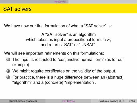
We have now our first formulation of what a “SAT solver” is:

A “SAT solver” is an algorithmwhich takes as input a propositional formula F ,

and returns “SAT” or “UNSAT”.

We will see important refinements on this formulations:1 The input is restricted to “conjunctive normal form” (as for our

example).2 We might require certificates on the validity of the output.3 For practice, there is a huge difference between an (abstract)

“algorithm” and a (concrete) “implementation”.


Introduction

Remarks on certificates

If a SAT solver returns “SAT” for input F , then usually we want to seethe satisfying assignment, a setting for the variables in F makingF = 1 true.

These satisfying assignments are the (standard) certificates forthe output “SAT”.They are short!Certificates for output “UNSAT” are also needed.They seem to be very long, and for harder examples are currentlynot feasible in practice.


Introduction

Remarks on tautology I

Since antiquity, tautologies have attracted a lot of attention.

These are boolean formulas F which are always true (i.e., 1).

For example(a ∧ (a→ b))→ b

is a tautology (the “modus ponens”).

Our example (a ∨ ¬b) ∧ (¬a ∨ c) ∧ (b ∨ ¬c) is obviously not atautology: it can be falsified by setting, e.g., a = 0 and b = 1.

Having a SAT solver, we can check for being a tautology (or not):

F is a tautology if and only if ¬F is unsatisfiable.


Introduction

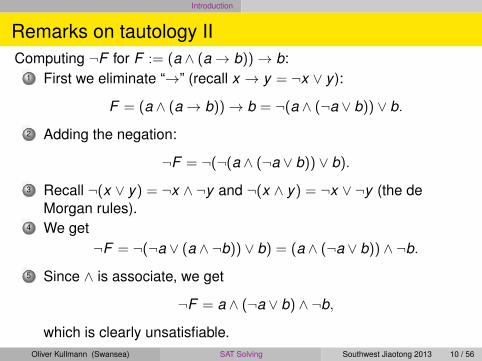
Remarks on tautology IIComputing ¬F for F := (a ∧ (a→ b))→ b:

1 First we eliminate “→” (recall x → y = ¬x ∨ y ):

F = (a ∧ (a→ b))→ b = ¬(a ∧ (¬a ∨ b)) ∨ b.

2 Adding the negation:

¬F = ¬(¬(a ∧ (¬a ∨ b)) ∨ b).

3 Recall ¬(x ∨ y) = ¬x ∧ ¬y and ¬(x ∧ y) = ¬x ∨ ¬y (the deMorgan rules).

4 We get¬F = ¬(¬a ∨ (a ∧ ¬b)) ∨ b) = (a ∧ (¬a ∨ b)) ∧ ¬b.

5 Since ∧ is associate, we get

¬F = a ∧ (¬a ∨ b) ∧ ¬b,

which is clearly unsatisfiable.Oliver Kullmann (Swansea) SAT Solving Southwest Jiaotong 2013 10 / 56

Introduction

It’s just a finite problem ...

What the fuss about a trivial problem like satisfiability – we can just tryout all of the finitely many possible solutions!

If we have n variables in F , then there are 2n assignments of 0,1to the variables.So for input F we have a trivial algorithm solving SAT, which takes

O(`(F ) · 2n(F ))

many steps (`(F ) is the length of the input).This algorithm also enumerates all possible solutions.

All problems solved?


Introduction

We can (and must) do better

A practical SAT problem has typically at least n = 1000:

21000 = 1.0715 · · · · 10301.

And many problems of industrial relevance have n ≈ 106 or evenn ≈ 109.

And we can solve (many) of these problems.


Introduction

SAT solving

SAT solving has evolved in an astounding fashion:With the development of practical SAT solving in the last decade, itgot a huge influence on verification.Especially the design of modern microchips wouldn’t be possiblewithout these algorithms.Some speak of the “SAT revolution”. (Though it’s hidden — it’stechnical, mathematical, not “glamorous”.)

See the SAT handbook Biere, Heule, van Maaren, and Walsh [1] forbasic information.

Theoretically we are much behind.However I believe a beautiful (mathematical) theory on SAT iswaiting to be discovered.That theory should also enable (still) much better SAT solving.


Introduction

Outline

1 Introduction

2 History

3 BackgroundClause-setsPartial assignments

4 Basic methodsBacktrackingForced assignmentsAutarkiesClause learning

5 Future

6 Conclusion


History

5 phases of SAT

1 Development of propositional logic, starting with the Greeks,especially the Stoics (around 300 BCE).

2 Boolean equations: starting with George Boole’s (1815-1864)book [2] from 1854.

3 Circuits: starting with Claude Shannon’s master thesis from 1937.4 NP-completeness: starting with Stephen Cook’s proof from 1971

that SAT is NP-complete [3].5 Turning NP-completeness from its head to its feet: SAT can be

used efficiently, and many other problems can be efficientlyreduced to it. This latest phase started around 2000.


http://en.wikipedia.org/wiki/Stoicism#Propositional_logic

http://en.wikipedia.org/wiki/George_Boole

http://en.wikipedia.org/wiki/Claude_Shannon#Boolean_theory_and_beyond

http://en.wikipedia.org/wiki/Stephen_Cook

History

NP-completeness

Boolean equations have the following properties:It might not be straightforward to find a solution, but to check,whether an alleged solution is really one, can be done efficiently.And if there is a solution at all, then there exists one which is (atmost) of similar size as the size of the equation itself.

This means that the (algorithmic) decision problem of deciding whethera boolean equation is solvable (satisfiable) or not is in NP.

The NP-completeness of this decision problem means,that every other problem in NP is efficiently reducible to it.


History

P versus NP

The NP-completeness of Boolean Equations (BE) means:

If we have a good solver for it, then,with some overhead, we have a good solver

for every problem in NP.

How well we can solve BE is representative for NP!The famous “P versus NP” problem is thus precisely the question,whether BE (or SAT) can be solved in polynomial time.It is considered as one of the most important open problems inmathematics, and definitely it is the main open problems incomputer science.

See 7 Millennium Problems.


http://www.claymath.org/millennium/P_vs_NP/

History

Remarks on ideology

In the 80s and 90s emerged the ideology of“efficient” or “feasible” means “poly-time”.Worst, not-poly-time means “infeasible”.Just a term was defined, “infeasible”, which could also have beencalled “Bierseidel” (according to Hilbert). But this term was notused formally, but with “deep meaning”.The disastrous consequence of that was, that the 80’s and 90’swere dominated by the rejection of SAT solving as “infeasible”,and instead probabilistic or approximative approaches weredominant (which didn’t add much to SAT solving).And mathematicians learned to abhor “combinatorial explosions”.It’s there, but you are supposed not to look at it ...

SAT is the theory of combinatorial explosion “at the edge”.


http://math.stackexchange.com/questions/56603/provenance-of-hilbert-quote-on-table-chair-beer-mug

History

Some other applications

Besides EDA (“Electronic Design Automation”) here are some otherapplications:

Verifying railway safety procedures and hardware.Computing numbers from Ramsey theory (especially van derWaerden numbers).Breaking cryptographic ciphers (cryptanalysis).Solving various (mathematical and non-mathematical) puzzles(latin squares etc.).


http://en.wikipedia.org/wiki/Electronic_design_automation

Background Clause-sets

The Conjunctive Normal Form (CNF)

We restrict our attention to the standard boolean basis ∨ , ∧ ,¬.Any formula F over this basis can be transformed into an equivalentformula which is a conjunctions of disjunctions of literals, where literalsare variables and their negations, using:

1 double negation is the identity: ¬¬F = F ;2 de Morgan rules to move the negations inwards;3 the distributive law

(a ∧ b) ∨ (c ∧ d) = (a ∨ c) ∧ (a ∨ d) ∧ (b ∨ c) ∧ (b ∨ d).To present the basics, I won’t rely on these mechanisms from logic:

I use an algebraic (not “logical”) construction of the basic objects.CNFs are treated as clause-sets, which are considered as(precise) combinatorial objects, as generalised hypergraphs.



Variables and literals I

We assume an infinite set VA of variables.We define LIT := VA× {0,1}.The elements of LIT are called literals.We identify the literals (v ,0) with the variables v .var((v , ε)) := v and sgn((v , ε)) := ε.We have a fixed-point free involution on LIT :

(v , ε) ∈ LIT 7→ (v , ε) := (v ,1− ε) ∈ LIT .

Literal x is the complement of literal x .The defining properties of complementation are

x 6= x , x = x .



Variables and literals II

For implementation purposes typically the following choice isappropriate, using N = {1,2, . . .}:

1 VA := N2 LIT := Z \ {0}.3 x ∈ LIT 7→ x := −x ∈ LIT .

Nothing is lost if you just use this model.Remarks:

In general, the structure given by variables and literals is just afree Z2-set LIT , freely generated by VA.For systematic purposes it can also be useful to allow arbitraryZ2-sets, i.e., to allow that the complementation has fixed points.Such degenerations can be useful to round off certainconstructions.



Clause-sets I

For L ⊆ LIT let L := {x : x ∈ L}.A clause is a finite and clash-free set of literals, the set of clausesis denoted by

CL := {C ⊂ LIT | C finite ∧ C ∩ C = ∅}.

The simplest clause is ⊥ := ∅ ∈ CL, the empty clause.A clause-set is a set of clauses, the set of all clause-sets isdenoted by CLS := P(CL).The simplest clause-set is > := ∅ ∈ CLS, the empty clause-set.

From now on only finite clause-sets are considered, since we areconcentrating on algorithmic issues.



Clause-sets II

For example {{a,b}, {a, c,d},⊥

}is a clause-set. When writing such examples, it is typically understoodthat, e.g., a,b, c,d are pairwise different variables.

If considering literals as integers, then:

Clauses are just finite sets C ⊂ Z \ {0} of non-zero integers, suchthat for x ∈ C we have −x /∈ C.

Clause-sets are just finite sets of such clauses.

We ask for clauses to be clash-free, since clauses containing clasheswould be tautologies. For some constructions however it can bebeneficial to allow such degenerations.



Clause-sets III

To spell out the interpretation:

F ={{a,b}, {b, c}, {a, c}

}︸︷︷︸clause-set

∼ (a ∨ b) ∧ (¬b ∨ c) ∧ (¬a ∨ ¬c)︸︷︷︸CNF

.

The interpretation of a clause-set as a CNF is the defaultinterpretation, and guides the definitions.



Variables and literals in clause-sets

For a clause C ∈ CL: var(C) := {var(x) : x ∈ C}.

For F ∈ CLS:

var(F ) :=⋃

C∈F

var(C)

lit(F ) := var(F ) ∪ var(F )

i.e.,var(F ) is the set of variables of Flit(F ) is the set of (possible) literals of F .

Note that the actually occurring literals are given by⋃

F .



Measures

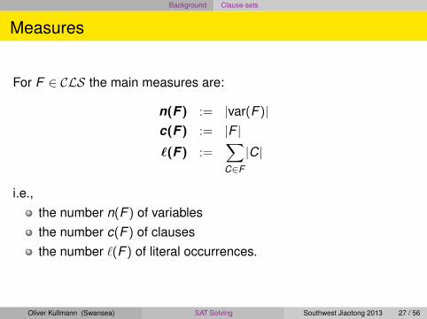
For F ∈ CLS the main measures are:

n(F ) := |var(F )|c(F ) := |F |`(F ) :=

∑C∈F

|C|

i.e.,the number n(F ) of variablesthe number c(F ) of clausesthe number `(F ) of literal occurrences.


Background Partial assignments

Partial assignments

A “partial assignment” maps some variables to {0,1} (“truthvalues”).The set of all partial assignments is PASS.The application of a partial assignment ϕ to a clause-set F isdenoted by ϕ ∗ F .

The theory of SAT can be understoodas the theory of the operation

of the monoid PASS on the set CLS.



PASS

A partial assignment is a map

ϕ : V → {0,1}

for some finite V ⊂ VA. We use var(ϕ) := V .

The set PASS of all partial assignments carries a monoid structure:1 The composition ◦ : PASS × PASS → PASS is defined forϕ,ψ ∈ PASS as follows:

1 var(ψ ◦ ϕ) = var(ψ) ∪ var(ϕ)2 for v ∈ var(ψ ◦ ϕ) the result is obtained by using ϕ(v) is possible,

and only if this is not possible then ψ(v) is used.2 ◦ is associative (and not commutative).3 The neutral element is 〈〉 := ∅ ∈ PASS.



Extending partial assignments to literals

For a variable v ∈ var(ϕ) we define

ϕ(v) := ϕ(v) := 1− ϕ(v).

Thus we have for literals x with var(x) ∈ var(ϕ):

ϕ(x) = ϕ(x).



∗ : PASS × CLS → CLS

The application of a partial assignment ϕ ∈ PASS to a clause-setF ∈ CLS is denoted by

ϕ ∗ F ∈ CLS,

and is defined as

ϕ ∗ F :={{x ∈ C : ϕ(x) 6= 0} | C ∈ F ∧ ∀ x ∈ C : ϕ(x) 6= 1

}.

That is:First all satisfied clauses are removed (i.e., clauses containing atleast one literal set to 1).From the remaining clauses all falsified literals are removed.



SAT and UNSAT

The two central definitions:

SAT := {F ∈ CLS | ∃ϕ ∈ PASS : ϕ ∗ F = >}USAT := CLS \ SAT .

The two basic examples:> ∈ SAT , since 〈〉 ∗ > = >.{⊥} ∈ USAT , since ⊥ can not be satisfied.More generally, every F with ⊥ ∈ F is unsatisfiable.



Examples

Consider F :={{a,b}, {b, c}, {a, c}

}.

〈b → 1〉 ∗ F ={{c}, {a, c}

}〈b, c → 1〉 ∗ F = >.

Thus F ∈ SAT .

〈a→ 1〉 ∗ F ={{b}, {b, c}, {c}

}〈a→ 1, c → 0〉 ∗ F =

{{b}, {b},⊥

}∈ USAT

〈a→ 1, c → 1〉 ∗ F ={{b}

}〈a→ 1, c → 1,b → 1〉 ∗ F = >



The fundamental laws

(ψ ◦ ϕ) ∗ F = ψ ∗ (ϕ ∗ F )

ϕ ∗ > = >〈〉 ∗ F = F

ϕ ∗ (F ∪G) = (ϕ ∗ F ) ∪ (ϕ ∗G).

Additionally:var(ϕ ∗ F ) ⊆ var(F ) \ var(ϕ).Thus, if var(F ) ⊆ var(ϕ), then ϕ ∗ F ∈ {>, {⊥}}.



The special interpretation

If LIT = Z \ {0}:We can identify partial assignments ϕ with finite sets of non-zerointegers, not containing x and −x at the same time.These are the literals set to true by ϕ.ϕ is a satisfying assignment for F iff ϕ has non-empty intersectionwith every element of F .


Basic methods Backtracking

Backtracking

The basic method is splitting on a variable: For F ∈ CLS andv ∈ var(F ) holds

F ∈ SAT if and only if〈v → 0〉 ∗ F ∈ SAT or 〈v → 1〉 ∗ F ∈ SAT .

Note that v /∈ 〈v → ε〉 ∗ F , and thus this procedure terminates.

Also note for the recursion basis (as already noticed):

var(F ) = ∅ ⇔ F ∈ {>, {⊥}}.


Basic methods Backtracking

The most basic SAT-algorithm

In C++ pseudo-code:

bool A0(CLS F) {i f ( { } i n F ) return fa lse ;i f (F == { } ) return true ;choose v i n var (F ) ; / / branching v a r i a b l echoose e i n { 0 , 1 } ; / / f i r s t branchi f (A0( <v −> e> ∗ F) ) return true ;else return A0( <v −> (1−e ) > ∗ F) ;

}

With a reasonable heuristics, already this algorithmcan be much faster than 2n.


Basic methods Forced assignments

Forced assignments

An assignment 〈x → 1〉 for a literal x and F ∈ CLSis called forced, if 〈x → 0〉 ∗ F ∈ USAT .

Thus 〈x → 1〉 ∗ F is sat-equivalent to F .So we can (and should!) apply the partial assignment 〈x → 1〉.The problem in general is, that detection of a forced assignment iscoNP-complete.So special cases need to be considered.

The easiest case is ⊥ ∈ F (why?).

Then comes {x} ∈ F .



Unit-clause propagation

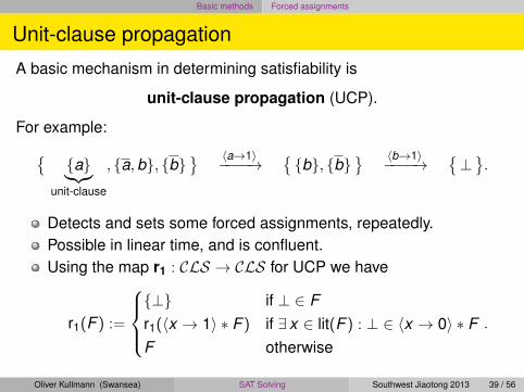
A basic mechanism in determining satisfiability is

unit-clause propagation (UCP).

For example:{{a}︸︷︷︸

unit-clause

, {a,b}, {b}} 〈a→1〉−−−−→

{{b}, {b}

} 〈b→1〉−−−−→{⊥}.

Detects and sets some forced assignments, repeatedly.Possible in linear time, and is confluent.Using the map r1 : CLS → CLS for UCP we have

r1(F ) :=

{⊥} if ⊥ ∈ Fr1(〈x → 1〉 ∗ F ) if ∃ x ∈ lit(F ) : ⊥ ∈ 〈x → 0〉 ∗ FF otherwise

.



Generalised unit-clause propagation

Kullmann [7, 8] introduced the notion of

generalised unit-clause propagationrk : CLS → CLS, k ∈ N0.

r0(F ) :=

{{⊥} if ⊥ ∈ FF otherwise

r1(F ) =

{r1(〈x → 1〉 ∗ F ) if ∃ x ∈ lit(F ) : r0(〈x → 0〉 ∗ F ) = {⊥}F otherwise

rk (F ) :=

{rk (〈x → 1〉 ∗ F ) if ∃ x ∈ lit(F ) : rk−1(〈x → 0〉 ∗ F ) = {⊥}F otherwise

.

rk (F ) can be computed in time `(F ) · n(F )2k−2.



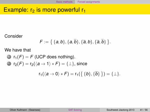
Example: r2 is more powerful r1

ConsiderF :=

{{a,b}, {a,b}, {a,b}, {a,b}

}.

We have that1 r1(F ) = F (UCP does nothing).2 r2(F ) = r2(〈a→ 1〉 ∗ F ) = {⊥}, since

r1(〈a→ 0〉 ∗ F ) = r1({{b}, {b}

}) = {⊥}.



Algorithm scheme Ak

For some fixed k ∈ N0:

bool Ak (CLS F) {F = r_k (F ) ;i f (F == { { } } ) return fa lse ;i f (F == { } ) return true ;choose v i n var (F ) ; / / branching v a r i a b l echoose e i n { 0 , 1 } ; / / f i r s t branchi f ( Ak( <v −> e> ∗ F) ) return true ;else return Ak( <v −> (1−e ) > ∗ F) ;

}

For k = 0 we get A0.For decent performance at least k = 1.k = 2,3 (typically not used completely) was restricted to“look-ahead” SAT solvers in the past (see [5, 10]), but k = 2started to become used by “conflict-driven” solvers recently.


Basic methods Autarkies

Autarkies

Dual to forced assignments (in a sense) are “autarkies”:

An autarky for a clause-set F is a partial assignment ϕ whichsatisfies every clause C ∈ F it touches (i.e., var(ϕ) ∩ var(C) 6= ∅).Again, for an autarky ϕ the result ϕ ∗ F of “autarky reduction” issat-equivalent to F (note that ϕ ∗ F ⊆ F ).Detection of autarkies is NP-complete.So, again, schemes for restricted autarkies are needed.


Basic methods Autarkies

Pure literals and beyond

The simplest case of autarkies are “pure literals”:

If for a literal x we have x /∈⋃

F ,then x is called pure for F ,

and 〈x → 1〉 is an autarky for F .

This is just the beginning, and a nice theory of autarky has emerged;see [6].


Basic methods Clause learning

Clause learning

A look-ahead solver is an extension of scheme Ak, using alsoautarkies and other reductions.

They are good for cases which are essentially hard, and sosystematic work is required.However they are typically less good for examples with a lot of“special structure”.The “SAT revolution”, which took place in the last decade, is basedon solvers capable of exploiting such structures.Since such structures are typical for practical examples.

This new type of solver is called conflict-driven (or “CDCL” –conflict-driven clause-learning); see [11].



The basic idea

A look-ahead solvers has the organisation of the search (the splitting-or backtracking-tree) externally, while a conflict-driven solverinternalises it:

If at the end of a brancha partial assignment ϕ yields ⊥ ∈ ϕ ∗ F ,

then we might “learn” the “cause” of this “conflict”.

And if the learning result is a clause, then we can add it to F .



How can this work?

What else can there be in ϕ —more than the falsified clause C ∈ F (i.e., ϕ ∗ {C} = {⊥})

(which we already have)?

The point is that ϕ does not only contain “decision variables” (thebranch variables), but also forced assignments, typically by r1.

Via this “conflict analysis”,thus we might replace assignments to variables in C

by some other assignments — we learned something!



Learning a clause

It boils down to the circumstance,

that from ⊥ ∈ ϕ ∗ F we can infer,via conflict-analysis,

ϕ′ ∗ F ∈ USAT for some ϕ′ ⊆ ϕ.

Now we can learn the negation of ϕ′. For example

ϕ′ = 〈a→ 0,b → 1〉

means “a = 0 ∧ b = 1”. Negation yields “a = 1 ∨ b = 0” — a clause!So we learn the clause Cϕ′ .Cϕ′ contains precisely the literals set to 0 by ϕ′.For the example we have Cϕ′ = {a,b}.“Learning” means F ; F ∪ {Cϕ′}.



An example

Consider

F :={{a,b, c}, {a,b, c}, {a,b, c}, {a,b, c},

{a,b, c}, {a,b, c}, {a,b, c}, {a,b, c}}.

1 We start with a→ 0 (first decision).2 r1 yields nothing.3 Then we assign b → 0 (second decision).4 Now r1 yields c → 1.5 So we have now ϕ = 〈a→ 0,b → 0, c → 1〉.6 We have ⊥ ∈ ϕ ∗ F .7 Via conflict analysis we get ϕ′ := 〈a→ 0,b → 0〉.8 So we learn Cϕ′ = {a,b}.


Future

Main challenges related to SAT solving


Future

I Develop a true hybrid solver

The 90’s were the time of look-ahead and local-search solvers.The last decade then was the time of conflict-driven solvers.It is clear, that no scheme dominates the others.A “true” combination of these three schemes is needed (not just a“hybrid” as an ad-hoc mixture).

For some first remarks, connecting look-ahead and conflict-driven, see[9].


Future

II Theory of good representations

Currently just ad-hoc methods for representing computationalproblems as SAT problems are used:

A theory is needed here.The practical applications should be developed together with newSAT solvers (which might be needed to understand betterrepresentations).

For some approaches, see [4].


Future

III Theory of heuristics

Heuristics are dominated by engineering approaches —mathematics is needed!Especially the heuristics for conflict-driven solvers are obscure.

See [10] for a foundation for look-ahead solvers.


Future

IV Understanding!

I believe it is possible to understand the fundamental patterns ofunsatisfiability.Also a much refined proof theory is needed, taking specialproblem structures into account.SAT is more complicated than UNSAT here; I believe consideringSAT as a kind of “limit” of UNSAT is the right approach.


Conclusion

Summary and outlook

I I believe most of the interesting things in SAT are still to come!II Especially theory is needed.


Conclusion

End

(references on the remaining slides).

For my papers seehttp://cs.swan.ac.uk/~csoliver/papers.html.


http://cs.swan.ac.uk/~csoliver/papers.html

Conclusion

Bibliography I

[1] Armin Biere, Marijn J.H. Heule, Hans van Maaren, and TobyWalsh, editors. Handbook of Satisfiability, volume 185 of Frontiersin Artificial Intelligence and Applications. IOS Press, February2009. ISBN 978-1-58603-929-5.

[2] George Boole. An Investigation of The Laws of Thought, on whichare founded The Mathematical Theorie of Logic and Probabilities.Dover Publication, Inc., first published in 1958. ISBN0-486-60028-9; printing of the work originally published byMacmillan in 1854, with all corrections made within the text.

[3] Stephen A. Cook. The complexity of theorem-proving procedures.In Proceedings 3rd Annual ACM Symposium on Theory ofComputing, pages 151–158, 1971.


Conclusion

Bibliography II

[4] Matthew Gwynne and Oliver Kullmann. Towards a theory of goodSAT representations. Technical Report arXiv:1302.4421v3 [cs.AI],arXiv, March 2013.

[5] Marijn J. H. Heule and Hans van Maaren. Look-ahead based SATsolvers. In Biere et al. [1], chapter 5, pages 155–184. ISBN978-1-58603-929-5.

[6] Hans Kleine Büning and Oliver Kullmann. Minimal unsatisfiabilityand autarkies. In Biere et al. [1], chapter 11, pages 339–401.ISBN 978-1-58603-929-5. doi: 10.3233/978-1-58603-929-5-339.

[7] Oliver Kullmann. Investigating a general hierarchy of polynomiallydecidable classes of CNF’s based on short tree-like resolutionproofs. Technical Report TR99-041, Electronic Colloquium onComputational Complexity (ECCC), October 1999.


Conclusion

Bibliography III

[8] Oliver Kullmann. Upper and lower bounds on the complexity ofgeneralised resolution and generalised constraint satisfactionproblems. Annals of Mathematics and Artificial Intelligence, 40(3-4):303–352, March 2004.

[9] Oliver Kullmann. Present and future of practical SAT solving. InNadia Creignou, Phokion Kolaitis, and Heribert Vollmer, editors,Complexity of Constraints: An Overview of Current ResearchThemes, volume 5250 of Lecture Notes in Computer Science(LNCS), pages 283–319. Springer, 2008. doi:10.1007/978-3-540-92800-3_11. ISBN-10 3-540-92799-9.

[10] Oliver Kullmann. Fundaments of branching heuristics. In Biereet al. [1], chapter 7, pages 205–244. ISBN 978-1-58603-929-5.doi: 10.3233/978-1-58603-929-5-205.


Conclusion

Bibliography IV

[11] Joao P. Marques-Silva, Ines Lynce, and Sharad Malik.Conflict-driven clause learning SAT solvers. In Biere et al. [1],chapter 4, pages 131–153. ISBN 978-1-58603-929-5.


sat solving: theory and practice of efficient...

Documents