sas programming dongfeng li some statistics sas programming in clinical trials ... · sas...
TRANSCRIPT

SAS Programmingin Clinical TrialsChapter 3. SAS
STAT
Dongfeng Li
Some StatisticsBackground
Descriptivestatistics: conceptsand programs
Comparing theMean
Analysis ofVariance
SAS Programming in Clinical TrialsChapter 3. SAS STAT
Dongfeng Li
Autumn 2010
SAS Programmingin Clinical TrialsChapter 3. SAS
STAT
Dongfeng Li
Some StatisticsBackground
Descriptivestatistics: conceptsand programs
Comparing theMean
Analysis ofVariance
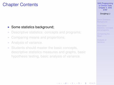
Chapter Contents
I Some statistics background;I Descriptive statistics: concepts and programs;I Comparing means and proportions;I Analysis of variance.I Students should master the basic concepts,
descriptive statistics measures and graphs, basichypothesis testing, basic analysis of variance.

SAS Programmingin Clinical TrialsChapter 3. SAS
STAT
Dongfeng Li
Some StatisticsBackground
Descriptivestatistics: conceptsand programs
Comparing theMean
Analysis ofVariance
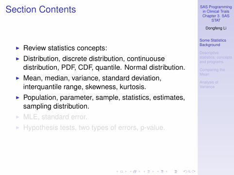
Section Contents
I Review statistics concepts:I Distribution, discrete distribution, continuouse
distribution, PDF, CDF, quantile. Normal distribution.I Mean, median, variance, standard deviation,
interquantile range, skewness, kurtosis.I Population, parameter, sample, statistics, estimates,
sampling distribution.I MLE, standard error.I Hypothesis tests, two types of errors, p-value.

SAS Programmingin Clinical TrialsChapter 3. SAS
STAT
Dongfeng Li
Some StatisticsBackground
Descriptivestatistics: conceptsand programs
Comparing theMean
Analysis ofVariance
Section Contents
I Review statistics concepts:I Distribution, discrete distribution, continuouse
distribution, PDF, CDF, quantile. Normal distribution.I Mean, median, variance, standard deviation,
interquantile range, skewness, kurtosis.I Population, parameter, sample, statistics, estimates,
sampling distribution.I MLE, standard error.I Hypothesis tests, two types of errors, p-value.

SAS Programmingin Clinical TrialsChapter 3. SAS
STAT
Dongfeng Li
Some StatisticsBackground
Descriptivestatistics: conceptsand programs
Comparing theMean
Analysis ofVariance
Distribution
I Random Variable:I Discrete, such as sex, patient/control, age group.I Continuous, such as weight, blood pressure.
I Distribution: used to describe the relative chance oftaking some value.
I For discrete variable X , use P(X = xi ), where {xi}are the value set of X . Called probability massfunction(PMF).
I For continuous variable X , use the probability densityfunction(PDF) f (x), whereP(X ∈ (x − ε, x + ε) ∝ f (x)(2ε).

SAS Programmingin Clinical TrialsChapter 3. SAS
STAT
Dongfeng Li
Some StatisticsBackground
Descriptivestatistics: conceptsand programs
Comparing theMean
Analysis ofVariance
CDF
I Cumulative distribution function(CDF) F (x):
F (x) = P(X ≤ x)
P(x ∈ (a,b]) = F (b)− F (a)
I For discrete distribution,
F (x) =∑xi≤x
P(X = xi)
I For continuous distribution,
F (x) =
∫ x
−∞f (t)dt

SAS Programmingin Clinical TrialsChapter 3. SAS
STAT
Dongfeng Li
Some StatisticsBackground
Descriptivestatistics: conceptsand programs
Comparing theMean
Analysis ofVariance
Quantile function
I Quantile function: the inverse of CDF
q(p) = F−1(p),p ∈ (0,1)
if F (x) is 1-1 mapping.I Generally, q(p) = xp where
P(X ≤ xp) ≥ p,P(X ≥ xp) ≥ 1− p
(xp can be non-unique.)
SAS Programmingin Clinical TrialsChapter 3. SAS
STAT
Dongfeng Li
Some StatisticsBackground
Descriptivestatistics: conceptsand programs
Comparing theMean
Analysis ofVariance
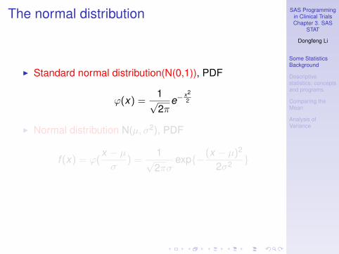
The normal distribution
I Standard normal distribution(N(0,1)), PDF
ϕ(x) =1√2π
e−x22
I Normal distribution N(µ, σ2), PDF
f (x) = ϕ(x − µσ
) =1√2πσ
exp{−(x − µ)2
2σ2 }

SAS Programmingin Clinical TrialsChapter 3. SAS
STAT
Dongfeng Li
Some StatisticsBackground
Descriptivestatistics: conceptsand programs
Comparing theMean
Analysis ofVariance
Numerical charasteristics
I PDF is a curve with infinite number of points.I We can use some numbers to describe the key part
of a distribution.I Firstly, the location measurement.
I The mean EX .I The meadian, x0.5 = q(0.5) where
P(x ≤ x0.5) ≥ 0.5,P(x ≥ x0.5) ≥ 0.5
(can be non-unique).I Variability measurement.
I The standard deviation σX =√
E(X − EX )2.I Interquantile range q(0.75)− q(0.25).

SAS Programmingin Clinical TrialsChapter 3. SAS
STAT
Dongfeng Li
Some StatisticsBackground
Descriptivestatistics: conceptsand programs
Comparing theMean
Analysis ofVariance
I Shape characteristics. Skewness
E(
X − EXσX
)3
I Symmetric, left-skewed, right-skewed density.I Shape characteristics. Kurtosis
E(
X − EXσX
)4
− 3
I Heavy tail problem.I Multimodel distribution. E.g., the weight of 10 year
old and 20 year old mixed together.

SAS Programmingin Clinical TrialsChapter 3. SAS
STAT
Dongfeng Li
Some StatisticsBackground
Descriptivestatistics: conceptsand programs
Comparing theMean
Analysis ofVariance
Population
I A population is modeled by a random variable or adistribution.
I Population parameters: unknown numbers whichcould decide the distribution. E.g., for N(µ, σ2)population, (µ, σ2) are the two unknown populationparameters.

SAS Programmingin Clinical TrialsChapter 3. SAS
STAT
Dongfeng Li
Some StatisticsBackground
Descriptivestatistics: conceptsand programs
Comparing theMean
Analysis ofVariance
Sample
I A sample(typically) is n observations drawindependently from the population, X1,X2, . . . ,Xn.
I A sample can be regarded as n numbers, or n iidrandom variables.
I Statistics: calculate some values to estimate thedistribution of the population. Can be regarded as arandom variable. Such as sample mean, samplestandard deviation. Can be used to estimateunknown population parameters, called estimates.
I Sampling distribution: The distribution of anestimator or other statistic. E.g., if X1, . . . ,Xn is asample from N(µ, σ2), then X ∼ N(µ, σ2/n).

SAS Programmingin Clinical TrialsChapter 3. SAS
STAT
Dongfeng Li
Some StatisticsBackground
Descriptivestatistics: conceptsand programs
Comparing theMean
Analysis ofVariance
MLE(Maximimum Likelihood Estimate)
I MLE is a commonly used parameter estimationmethod. For random sample X1,X2, . . . ,Xn frompopulation X , if PDF of PMF of X is f (x ;β), then
β = arg maxβ
L(β) = arg maxβ
n∏i=1
f (Xi ;β)
is called the MLE of the unknow parameter β.I Under some conditions, when the sample size
n→∞, β has a limiting(approximate) distributionN(β, σ2
β).

SAS Programmingin Clinical TrialsChapter 3. SAS
STAT
Dongfeng Li
Some StatisticsBackground
Descriptivestatistics: conceptsand programs
Comparing theMean
Analysis ofVariance
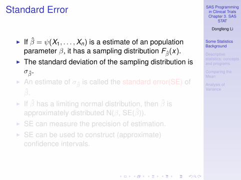
Standard Error
I If β = ψ(X1, . . . ,Xn) is a estimate of an populationparameter β, it has a sampling distribution Fβ(x).
I The standard deviation of the sampling distribution isσβ.
I An estimate of σβ is called the standard error(SE) ofβ.
I If β has a limiting normal distribution, then β isapproximately distributed N(β, SE(β)).
I SE can measure the precision of estimation.I SE can be used to construct (approximate)
confidence intervals.
SAS Programmingin Clinical TrialsChapter 3. SAS
STAT
Dongfeng Li
Some StatisticsBackground
Descriptivestatistics: conceptsand programs
Comparing theMean
Analysis ofVariance
Standard Error
I If β = ψ(X1, . . . ,Xn) is a estimate of an populationparameter β, it has a sampling distribution Fβ(x).
I The standard deviation of the sampling distribution isσβ.
I An estimate of σβ is called the standard error(SE) ofβ.
I If β has a limiting normal distribution, then β isapproximately distributed N(β, SE(β)).
I SE can measure the precision of estimation.I SE can be used to construct (approximate)
confidence intervals.

SAS Programmingin Clinical TrialsChapter 3. SAS
STAT
Dongfeng Li
Some StatisticsBackground
Descriptivestatistics: conceptsand programs
Comparing theMean
Analysis ofVariance
Hypothesis Tests
I To test the null hypothesis H0 agaist the alternativehypothesis Ha on the population;
I Given sample X1,X2, . . . ,Xn from population F (x ; θ),construct some statistic ξ, whose distribution doesnot depend on θ, but its value can indicate thepossible choice of H0 or Ha.
I Traditionally, we first choose an significance level α,then we find a rejection area W , wheresupH0
P(ξ ∈W ) ≤ α. We reject H0 when ξ ∈W .

SAS Programmingin Clinical TrialsChapter 3. SAS
STAT
Dongfeng Li
Some StatisticsBackground
Descriptivestatistics: conceptsand programs
Comparing theMean
Analysis ofVariance
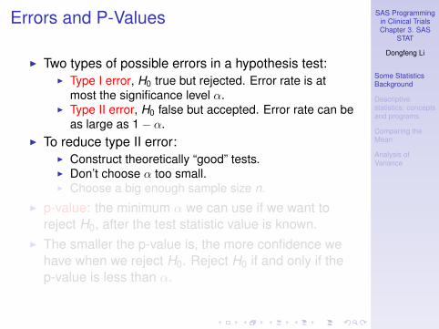
Errors and P-Values
I Two types of possible errors in a hypothesis test:I Type I error, H0 true but rejected. Error rate is at
most the significance level α.I Type II error, H0 false but accepted. Error rate can be
as large as 1− α.I To reduce type II error:
I Construct theoretically “good” tests.I Don’t choose α too small.I Choose a big enough sample size n.
I p-value: the minimum α we can use if we want toreject H0, after the test statistic value is known.
I The smaller the p-value is, the more confidence wehave when we reject H0. Reject H0 if and only if thep-value is less than α.

SAS Programmingin Clinical TrialsChapter 3. SAS
STAT
Dongfeng Li
Some StatisticsBackground
Descriptivestatistics: conceptsand programs
Comparing theMean
Analysis ofVariance
Errors and P-Values
I Two types of possible errors in a hypothesis test:I Type I error, H0 true but rejected. Error rate is at
most the significance level α.I Type II error, H0 false but accepted. Error rate can be
as large as 1− α.I To reduce type II error:
I Construct theoretically “good” tests.I Don’t choose α too small.I Choose a big enough sample size n.
I p-value: the minimum α we can use if we want toreject H0, after the test statistic value is known.
I The smaller the p-value is, the more confidence wehave when we reject H0. Reject H0 if and only if thep-value is less than α.

SAS Programmingin Clinical TrialsChapter 3. SAS
STAT
Dongfeng Li
Some StatisticsBackground
Descriptivestatistics: conceptsand programs
Comparing theMean
Analysis ofVariance
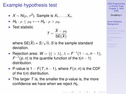
Example hypothesis test
I X ∼ N(µ, σ2). Sample is X1, . . . ,Xn.I H0 : µ ≤ µ0 ←→ Ha : µ > µ0.I Test statistic
T =X − µ0
SE(X )
where SE(X ) = S/√
n, S is the sample standarddeviation.
I Rejection area: W = {ξ > λ}, λ = F−1(1− α,n − 1),F−1(p,n) is the quantile function of the t(n − 1)distribution.
I P-value is 1− F (T ; n − 1), where F (x ; n) is the CDFof the t(n) distribution.
I The larger T is, the smaller the p-value is, the moreconfidence we have when we reject H0.

SAS Programmingin Clinical TrialsChapter 3. SAS
STAT
Dongfeng Li
Some StatisticsBackground
Descriptivestatistics: conceptsand programs
Comparing theMean
Analysis ofVariance
Example hypothesis test
I X ∼ N(µ, σ2). Sample is X1, . . . ,Xn.I H0 : µ ≤ µ0 ←→ Ha : µ > µ0.I Test statistic
T =X − µ0
SE(X )
where SE(X ) = S/√
n, S is the sample standarddeviation.
I Rejection area: W = {ξ > λ}, λ = F−1(1− α,n − 1),F−1(p,n) is the quantile function of the t(n − 1)distribution.
I P-value is 1− F (T ; n − 1), where F (x ; n) is the CDFof the t(n) distribution.
I The larger T is, the smaller the p-value is, the moreconfidence we have when we reject H0.

SAS Programmingin Clinical TrialsChapter 3. SAS
STAT
Dongfeng Li
Some StatisticsBackground
Descriptivestatistics: conceptsand programsDescriptive statistics
Summary statistics
Comparing theMean
Analysis ofVariance
Section Contents
I Measurment level of variables.I Descriptive statistics for nominal variables.I Descriptive statistics for interval variables.I Histograms, boxplots, QQ plots, probability plots,
stem-leaf plots.I Using PROC FREQ, PROC MEANS, PROC
UNIVARIATE.

SAS Programmingin Clinical TrialsChapter 3. SAS
STAT
Dongfeng Li
Some StatisticsBackground
Descriptivestatistics: conceptsand programsDescriptive statistics
Summary statistics
Comparing theMean
Analysis ofVariance
Measurement levels
I Nominal, such as sex, job type, race.I Ordinal, such as age group(child, youth, medium,
old), dose level(none, low, high).I Interval, such as weight, blood pressure, heart rate.
SAS Programmingin Clinical TrialsChapter 3. SAS
STAT
Dongfeng Li
Some StatisticsBackground
Descriptivestatistics: conceptsand programsDescriptive statistics
Summary statistics
Comparing theMean
Analysis ofVariance
Statistics for nominal variables
I The value set.I The count of each value(called frequency), and the
percentage.I Use a bar chart to show the distribution.

SAS Programmingin Clinical TrialsChapter 3. SAS
STAT
Dongfeng Li
Some StatisticsBackground
Descriptivestatistics: conceptsand programsDescriptive statistics
Summary statistics
Comparing theMean
Analysis ofVariance
Example: frequency table
Use PROC FREQ to list the value set and the frequencycounts, percents.
proc freq data=sasuser.class;tables sex;
run;
Gender
sex Frequency Percent CumulativeFrequency
CumulativePercent
F 9 47.37 9 47.37
M 10 52.63 19 100.00

SAS Programmingin Clinical TrialsChapter 3. SAS
STAT
Dongfeng Li
Some StatisticsBackground
Descriptivestatistics: conceptsand programsDescriptive statistics
Summary statistics
Comparing theMean
Analysis ofVariance
Example: bar chart
Use PROC GCHART to make a bar chart. hbar could bereplaced with vbar, hbar3d, vbar3d.
proc gchart data=sasuser.class;hbar sex;
run;

SAS Programmingin Clinical TrialsChapter 3. SAS
STAT
Dongfeng Li
Some StatisticsBackground
Descriptivestatistics: conceptsand programsDescriptive statistics
Summary statistics
Comparing theMean
Analysis ofVariance
Descriptive statistics for interval variables
I Location statistics: sample mean, sample median.I Variability statistics: sample standard deviation,
sample interquantile range, range, coefficient ofvariation.
I Sample skewness n(n−1)(n−2)
∑(yi−y
s
)3.
I Sample kurtosis n(n+1)(n−1)(n−2)(n−3)
∑(yi−y)4
s4 − 3(n−1)2
(n−2)(n−3)
I Moments, quantiles.
SAS Programmingin Clinical TrialsChapter 3. SAS
STAT
Dongfeng Li
Some StatisticsBackground
Descriptivestatistics: conceptsand programsDescriptive statistics
Summary statistics
Comparing theMean
Analysis ofVariance
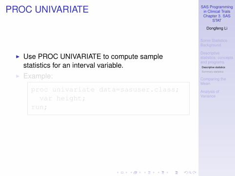
PROC UNIVARIATE
I Use PROC UNIVARIATE to compute samplestatistics for an interval variable.
I Example:
proc univariate data=sasuser.class;var height;
run;

SAS Programmingin Clinical TrialsChapter 3. SAS
STAT
Dongfeng Li
Some StatisticsBackground
Descriptivestatistics: conceptsand programsDescriptive statistics
Summary statistics
Comparing theMean
Analysis ofVariance
PROC UNIVARIATE
I Use PROC UNIVARIATE to compute samplestatistics for an interval variable.
I Example:
proc univariate data=sasuser.class;var height;
run;
SAS Programmingin Clinical TrialsChapter 3. SAS
STAT
Dongfeng Li
Some StatisticsBackground
Descriptivestatistics: conceptsand programsDescriptive statistics
Summary statistics
Comparing theMean
Analysis ofVariance
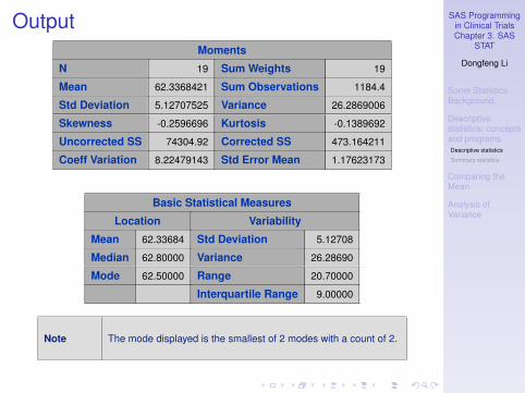
OutputMoments
N 19 Sum Weights 19
Mean 62.3368421 Sum Observations 1184.4
Std Deviation 5.12707525 Variance 26.2869006
Skewness -0.2596696 Kurtosis -0.1389692
Uncorrected SS 74304.92 Corrected SS 473.164211
Coeff Variation 8.22479143 Std Error Mean 1.17623173
Basic Statistical Measures
Location Variability
Mean 62.33684 Std Deviation 5.12708
Median 62.80000 Variance 26.28690
Mode 62.50000 Range 20.70000
Interquartile Range 9.00000
Note The mode displayed is the smallest of 2 modes with a count of 2.

SAS Programmingin Clinical TrialsChapter 3. SAS
STAT
Dongfeng Li
Some StatisticsBackground
Descriptivestatistics: conceptsand programsDescriptive statistics
Summary statistics
Comparing theMean
Analysis ofVariance
Tests for Location: Mu0=0
Test Statistic p Value
Student’s t t 52.99708 Pr > |t| <.0001
Sign M 9.5 Pr >= |M| <.0001
Signed Rank S 95 Pr >= |S| <.0001
SAS Programmingin Clinical TrialsChapter 3. SAS
STAT
Dongfeng Li
Some StatisticsBackground
Descriptivestatistics: conceptsand programsDescriptive statistics
Summary statistics
Comparing theMean
Analysis ofVariance
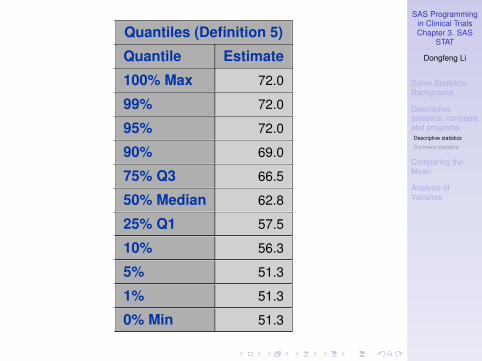
Quantiles (Definition 5)
Quantile Estimate
100% Max 72.0
99% 72.0
95% 72.0
90% 69.0
75% Q3 66.5
50% Median 62.8
25% Q1 57.5
10% 56.3
5% 51.3
1% 51.3
0% Min 51.3

SAS Programmingin Clinical TrialsChapter 3. SAS
STAT
Dongfeng Li
Some StatisticsBackground
Descriptivestatistics: conceptsand programsDescriptive statistics
Summary statistics
Comparing theMean
Analysis ofVariance
Extreme Observations
Lowest Highest
Value Obs Value Obs
51.3 7 66.5 6
56.3 4 66.5 19
56.5 1 67.0 12
57.3 13 69.0 10
57.5 18 72.0 16

SAS Programmingin Clinical TrialsChapter 3. SAS
STAT
Dongfeng Li
Some StatisticsBackground
Descriptivestatistics: conceptsand programsDescriptive statistics
Summary statistics
Comparing theMean
Analysis ofVariance
HistogramsI The histogram is a nonparametric estimate of the
population density function.I It divide the value set into intervals, and count the
percent of observations in each interval.I Example:
proc univariate data=sasuser.classnoprint;
var height; histogram;run;

SAS Programmingin Clinical TrialsChapter 3. SAS
STAT
Dongfeng Li
Some StatisticsBackground
Descriptivestatistics: conceptsand programsDescriptive statistics
Summary statistics
Comparing theMean
Analysis ofVariance
Examples of histograms
Skewness shown in histograms.

SAS Programmingin Clinical TrialsChapter 3. SAS
STAT
Dongfeng Li
Some StatisticsBackground
Descriptivestatistics: conceptsand programsDescriptive statistics
Summary statistics
Comparing theMean
Analysis ofVariance
Box plot
I Quantiles could be used to describe key distributioncharasteristics.
I The box plot shows the median, 1/4 and 3/4 quantile,and the minimum and maximum of a variable.
I The box holds the middle 50% range. Length is theIQR(inter quantile range).
I The wiskers extend to the minimum and themaximum; but the length of the wisker is not allowedto exceed 1.5 times the IQR.
I Points beyond wiskers are plotted as individualpoints. They are candidate for outliers.

SAS Programmingin Clinical TrialsChapter 3. SAS
STAT
Dongfeng Li
Some StatisticsBackground
Descriptivestatistics: conceptsand programsDescriptive statistics
Summary statistics
Comparing theMean
Analysis ofVariance
Example: boxplot of height

SAS Programmingin Clinical TrialsChapter 3. SAS
STAT
Dongfeng Li
Some StatisticsBackground
Descriptivestatistics: conceptsand programsDescriptive statistics
Summary statistics
Comparing theMean
Analysis ofVariance
proc sql;create view work._tmp_0 asselect height, 1 as _dummy_from sasuser.class;
title ;axis1 major=none value=none label=none;proc boxplot data=_tmp_0;
plot height*_dummy_ /boxstyle=skematiccboxfill=blue haxis=axis1;
run;

SAS Programmingin Clinical TrialsChapter 3. SAS
STAT
Dongfeng Li
Some StatisticsBackground
Descriptivestatistics: conceptsand programsDescriptive statistics
Summary statistics
Comparing theMean
Analysis ofVariance
Example: boxplot of GPA and CO
Skewness and possible outliers shown in boxplot.

SAS Programmingin Clinical TrialsChapter 3. SAS
STAT
Dongfeng Li
Some StatisticsBackground
Descriptivestatistics: conceptsand programsDescriptive statistics
Summary statistics
Comparing theMean
Analysis ofVariance
Grouped boxplot

SAS Programmingin Clinical TrialsChapter 3. SAS
STAT
Dongfeng Li
Some StatisticsBackground
Descriptivestatistics: conceptsand programsDescriptive statistics
Summary statistics
Comparing theMean
Analysis ofVariance
proc sort data=sasuser.gpa out=_tmp_1;by sex;
proc boxplot data=_tmp_1;plot gpa*sex /boxstyle=skematiccboxfill=blue;
run;

SAS Programmingin Clinical TrialsChapter 3. SAS
STAT
Dongfeng Li
Some StatisticsBackground
Descriptivestatistics: conceptsand programsDescriptive statistics
Summary statistics
Comparing theMean
Analysis ofVariance
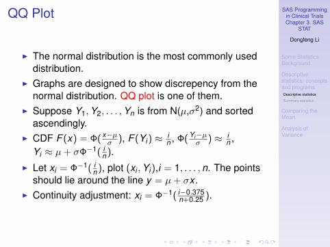
QQ Plot
I The normal distribution is the most commonly useddistribution.
I Graphs are designed to show discrepency from thenormal distribution. QQ plot is one of them.
I Suppose Y1,Y2, . . . ,Yn is from N(µ,σ2) and sortedascendingly.
I CDF F (x) = Φ(x−µσ ), F (Yi) ≈ i
n , Φ(Yi−µσ ) ≈ i
n ,Yi ≈ µ+ σΦ−1( i
n ).I Let xi = Φ−1( i
n ), plot (xi ,Yi),i = 1, . . . ,n. The pointsshould lie around the line y = µ+ σx .
I Continuity adjustment: xi = Φ−1( i−0.375n+0.25 ).

SAS Programmingin Clinical TrialsChapter 3. SAS
STAT
Dongfeng Li
Some StatisticsBackground
Descriptivestatistics: conceptsand programsDescriptive statistics
Summary statistics
Comparing theMean
Analysis ofVariance
QQ Plot
I The normal distribution is the most commonly useddistribution.
I Graphs are designed to show discrepency from thenormal distribution. QQ plot is one of them.
I Suppose Y1,Y2, . . . ,Yn is from N(µ,σ2) and sortedascendingly.
I CDF F (x) = Φ(x−µσ ), F (Yi) ≈ i
n , Φ(Yi−µσ ) ≈ i
n ,Yi ≈ µ+ σΦ−1( i
n ).I Let xi = Φ−1( i
n ), plot (xi ,Yi),i = 1, . . . ,n. The pointsshould lie around the line y = µ+ σx .
I Continuity adjustment: xi = Φ−1( i−0.375n+0.25 ).

SAS Programmingin Clinical TrialsChapter 3. SAS
STAT
Dongfeng Li
Some StatisticsBackground
Descriptivestatistics: conceptsand programsDescriptive statistics
Summary statistics
Comparing theMean
Analysis ofVariance
Example: QQ Plot of HEIGHTproc univariate
data=sasuser.class noprint;qqplot height /normal(mu=est sigma=est);
run;

SAS Programmingin Clinical TrialsChapter 3. SAS
STAT
Dongfeng Li
Some StatisticsBackground
Descriptivestatistics: conceptsand programsDescriptive statistics
Summary statistics
Comparing theMean
Analysis ofVariance
Example: Skewness in QQ Plot

SAS Programmingin Clinical TrialsChapter 3. SAS
STAT
Dongfeng Li
Some StatisticsBackground
Descriptivestatistics: conceptsand programsDescriptive statistics
Summary statistics
Comparing theMean
Analysis ofVariance
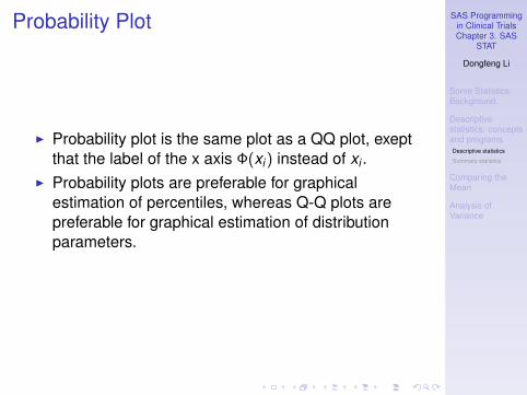
Probability Plot
I Probability plot is the same plot as a QQ plot, exeptthat the label of the x axis Φ(xi) instead of xi .
I Probability plots are preferable for graphicalestimation of percentiles, whereas Q-Q plots arepreferable for graphical estimation of distributionparameters.
SAS Programmingin Clinical TrialsChapter 3. SAS
STAT
Dongfeng Li
Some StatisticsBackground
Descriptivestatistics: conceptsand programsDescriptive statistics
Summary statistics
Comparing theMean
Analysis ofVariance
Probability Plot
I Probability plot is the same plot as a QQ plot, exeptthat the label of the x axis Φ(xi) instead of xi .
I Probability plots are preferable for graphicalestimation of percentiles, whereas Q-Q plots arepreferable for graphical estimation of distributionparameters.

SAS Programmingin Clinical TrialsChapter 3. SAS
STAT
Dongfeng Li
Some StatisticsBackground
Descriptivestatistics: conceptsand programsDescriptive statistics
Summary statistics
Comparing theMean
Analysis ofVariance
Example: Probability Plot of HEIGHTproc univariate
data=sasuser.class noprint;probplot height /normal(mu=est sigma=est);
run;

SAS Programmingin Clinical TrialsChapter 3. SAS
STAT
Dongfeng Li
Some StatisticsBackground
Descriptivestatistics: conceptsand programsDescriptive statistics
Summary statistics
Comparing theMean
Analysis ofVariance
The Stem-leaf Plot
I The stem-leaf plot is a text-based plot, which displayinformation like the histogram, but with detail on eachdata value. Each “leaf” corresponds to one datavalue.
I PROC UNIVARIATE has an option PLOT, whichgenerates text-based stem-leaf plot, boxplot and QQplot.

SAS Programmingin Clinical TrialsChapter 3. SAS
STAT
Dongfeng Li
Some StatisticsBackground
Descriptivestatistics: conceptsand programsDescriptive statistics
Summary statistics
Comparing theMean
Analysis ofVariance
proc univariate data=sasuser.classplot;
var height;run;
Stem Leaf #7 2 16 556679 66 022344 65 66789 55 1 1----+----+----+----+
Multiply Stem.Leaf by 10**+1
SAS Programmingin Clinical TrialsChapter 3. SAS
STAT
Dongfeng Li
Some StatisticsBackground
Descriptivestatistics: conceptsand programsDescriptive statistics
Summary statistics
Comparing theMean
Analysis ofVariance
PROC MEANS and PROC SUMMARY
I PROC MEANS and PROC SUMMARY are used toproduce summary statistics.
I They can display overall summary statistics andclassified summary statistics. PROC MEANSdisplays result by default; PROC SUMMARY needthe PRINT option to display result.
I They can output data sets with the summarystatistics. PROC SUMMARY is designed to do this,although PROC MEANS can do the same.
SAS Programmingin Clinical TrialsChapter 3. SAS
STAT
Dongfeng Li
Some StatisticsBackground
Descriptivestatistics: conceptsand programsDescriptive statistics
Summary statistics
Comparing theMean
Analysis ofVariance
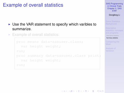
Example of overall statistics
I Use the VAR statement to specify which varibles tosummarize.
I Example of overall statistics:
proc means data=sasuser.class;var height weight;
run;proc summary data=sasuser.class print;
var height weight;run;

SAS Programmingin Clinical TrialsChapter 3. SAS
STAT
Dongfeng Li
Some StatisticsBackground
Descriptivestatistics: conceptsand programsDescriptive statistics
Summary statistics
Comparing theMean
Analysis ofVariance
Classified summary
I Use the CLASS statement to specify one or moreclass variables.
I Example:
proc means data=sasuser.class ;var height weight;class sex;
run;

SAS Programmingin Clinical TrialsChapter 3. SAS
STAT
Dongfeng Li
Some StatisticsBackground
Descriptivestatistics: conceptsand programsDescriptive statistics
Summary statistics
Comparing theMean
Analysis ofVariance
Other statistical measures
I PROC MEANS calculate summaries N, Mean,Standard Deviation, Minimum, Maximum by default.
I Use PROC MEANS options to specify otherstatistical measures.
I Example:
proc means data=sasuser.class MEAN VAR CV;var height weight;class sex;
run;

SAS Programmingin Clinical TrialsChapter 3. SAS
STAT
Dongfeng Li
Some StatisticsBackground
Descriptivestatistics: conceptsand programsDescriptive statistics
Summary statistics
Comparing theMean
Analysis ofVariance
Producing output datasets
I Use the OUTPUT statement to save the summarystatistics to an output dataset.
I Syntax:OUTPUT OUT=output-dataset keyword=
keyword= · · · / AUTONAME;I Where keyword is a name of some statistical
measure, like MEAN, STD, N, MIN, MAX, etc.I Example:
proc means data=sasuser.class MEAN VAR CV;var height weight;class sex;output out=res N= CV= / AUTONAME;
run;proc print data=res;run;

SAS Programmingin Clinical TrialsChapter 3. SAS
STAT
Dongfeng Li
Some StatisticsBackground
Descriptivestatistics: conceptsand programs
Comparing theMeanOne Sample Test of theMean
Comparing Two Groups
Paired Comparison
Comparing Proportions
Analysis ofVariance
Comparing the Mean
I One sample Z tests, t tests.I Two sample t tests.I The Wilcoxon rank sum test.I Paired t tests.I Comparing proportions: one sample and two sample.

SAS Programmingin Clinical TrialsChapter 3. SAS
STAT
Dongfeng Li
Some StatisticsBackground
Descriptivestatistics: conceptsand programs
Comparing theMeanOne Sample Test of theMean
Comparing Two Groups
Paired Comparison
Comparing Proportions
Analysis ofVariance
One Sample Z Test—Two-sided
I X ∼ N(µ, σ20), σ0 known.
I H0 : µ = µ0 ←→ Ha : µ 6= µ0
I Z = X−µ0σ0/√
nH0∼ N(0,1).
I W = {|Z | > λ}, λ = Φ−1(1− α/2).I p-value=2(1− Φ(|Z |).I Wald test: Based on the central limit theorem, to test
H0 : θ = θ0 ←→ Ha : θ 6= θ0, use W = θ−θ0SE(θ)
as thetest statistic, if W → N(0,1).

SAS Programmingin Clinical TrialsChapter 3. SAS
STAT
Dongfeng Li
Some StatisticsBackground
Descriptivestatistics: conceptsand programs
Comparing theMeanOne Sample Test of theMean
Comparing Two Groups
Paired Comparison
Comparing Proportions
Analysis ofVariance
One Sample Z Test—One-sided
I X ∼ N(µ, σ20), σ0 known.
I H0 : µ ≤ µ0 ←→ Ha : µ > µ0
I Z = X−µ0σ0/√
nµ=µ0∼ N(0,1).
I W = {Z > λ}, λ = Φ−1(1− α).I p-value=1− Φ(Z ).
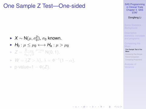
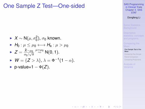

SAS Programmingin Clinical TrialsChapter 3. SAS
STAT
Dongfeng Li
Some StatisticsBackground
Descriptivestatistics: conceptsand programs
Comparing theMeanOne Sample Test of theMean
Comparing Two Groups
Paired Comparison
Comparing Proportions
Analysis ofVariance
Example: Z test
I For HEIGHT in SASUSER.CLASS, suppose σ0 = 5,µ0 = 65. One sample Z two-sided Z test:
proc means data=sasuser.classmean std n;
var height;output out=_tmp_1
mean=mu std=sigma n=n;run;

SAS Programmingin Clinical TrialsChapter 3. SAS
STAT
Dongfeng Li
Some StatisticsBackground
Descriptivestatistics: conceptsand programs
Comparing theMeanOne Sample Test of theMean
Comparing Two Groups
Paired Comparison
Comparing Proportions
Analysis ofVariance
data _null_;set _tmp_1;file print;mu0 = 65;sigma0 = 5;z = (mu - mu0)/(sigma0 / sqrt(n));pvalue = 2*(1 -
cdf(’normal’, abs(z)));put ’Z: ’ Z 12.4
’ Pr>|Z|: ’ pvalue PVALUE.;run;
Z: -2.3217 Pr>|Z|: 0.0202

SAS Programmingin Clinical TrialsChapter 3. SAS
STAT
Dongfeng Li
Some StatisticsBackground
Descriptivestatistics: conceptsand programs
Comparing theMeanOne Sample Test of theMean
Comparing Two Groups
Paired Comparison
Comparing Proportions
Analysis ofVariance
Example: Wald test
I Use the Wald test for HEIGHT mean.
data _null_;set _tmp_1;file print;mu0 = 65;sigma0 = sigma;z = (mu - mu0)/(sigma0 / sqrt(n));pvalue = 2*(1 -
cdf(’normal’, abs(z)));put ’Z: ’ Z 12.4
’ Pr>|Z|: ’ pvalue PVALUE.;run;Z: -2.2641 Pr>|Z|: 0.0236

SAS Programmingin Clinical TrialsChapter 3. SAS
STAT
Dongfeng Li
Some StatisticsBackground
Descriptivestatistics: conceptsand programs
Comparing theMeanOne Sample Test of theMean
Comparing Two Groups
Paired Comparison
Comparing Proportions
Analysis ofVariance
One-sample t Test for the Mean—Two-sided
I X ∼ N(µ, σ2), µ and σ unknown.I H0 : µ = µ0 ←→ Ha : µ 6= µ0.
I T = X−µ0S/√
nH0∼ t(n − 1).
I W = {|T | > λ}, λ = F−1t(n−1)(1− α/2).
I p-value=2(1− Ft(n−1)(|T |)).

SAS Programmingin Clinical TrialsChapter 3. SAS
STAT
Dongfeng Li
Some StatisticsBackground
Descriptivestatistics: conceptsand programs
Comparing theMeanOne Sample Test of theMean
Comparing Two Groups
Paired Comparison
Comparing Proportions
Analysis ofVariance
One-sample t Test for the Mean—One-sided
I X ∼ N(µ, σ2), µ and σ unknown.I H0 : µ ≤ µ0 ←→ Ha : µ > µ0.
I T = X−µ0S/√
nµ=µ0∼ t(n − 1).
I W = {T > λ}, λ = F−1t(n−1)(1− α).
I p-value=1− Ft(n−1)(T ).
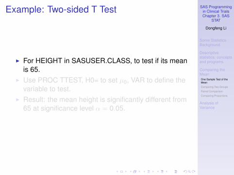
SAS Programmingin Clinical TrialsChapter 3. SAS
STAT
Dongfeng Li
Some StatisticsBackground
Descriptivestatistics: conceptsand programs
Comparing theMeanOne Sample Test of theMean
Comparing Two Groups
Paired Comparison
Comparing Proportions
Analysis ofVariance
Example: Two-sided T Test
I For HEIGHT in SASUSER.CLASS, to test if its meanis 65.
I Use PROC TTEST, H0= to set µ0, VAR to define thevariable to test.
I Result: the mean height is significantly different from65 at significance level α = 0.05.

SAS Programmingin Clinical TrialsChapter 3. SAS
STAT
Dongfeng Li
Some StatisticsBackground
Descriptivestatistics: conceptsand programs
Comparing theMeanOne Sample Test of theMean
Comparing Two Groups
Paired Comparison
Comparing Proportions
Analysis ofVariance
proc ttest data=sasuser.class H0=65;var height;
run;
Variable N Mean Std Devheight 19 62.337 5.1271
Variable DF t Value Pr > |t|height 18 -2.26 0.0362

SAS Programmingin Clinical TrialsChapter 3. SAS
STAT
Dongfeng Li
Some StatisticsBackground
Descriptivestatistics: conceptsand programs
Comparing theMeanOne Sample Test of theMean
Comparing Two Groups
Paired Comparison
Comparing Proportions
Analysis ofVariance
Example: One-sided T Test
I For the previous example, what if our question is “isthe mean height greater than 65?”
I Ha : µ > 65, which gives H0 : µ ≤ 65.I The program remains the same, but the p-value is
only for the two-sided test.I If X ≥ µ0, one sided p-value is half the two-sided
p-value.I If X < µ0, which means Ha is not sensible, we just
accept H0.I Since mean height is 62.337 < 65, Ha is not
sensible, we cannot conclude that mean height issignificantly larger than 65.
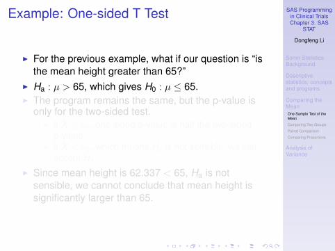

SAS Programmingin Clinical TrialsChapter 3. SAS
STAT
Dongfeng Li
Some StatisticsBackground
Descriptivestatistics: conceptsand programs
Comparing theMeanOne Sample Test of theMean
Comparing Two Groups
Paired Comparison
Comparing Proportions
Analysis ofVariance
Two Sample T-Test
I X and Y are two independent populations,X ∼ N(µ1, σ
2), Y ∼ N(µ2, σ2).
I Sample from X : X1, . . . ,Xn1 ; Sample from Y :Y1, . . . ,Yn2 .
I Two sided test: H0 : µ1 = mu2 ←→ Ha : µ1 6= µ2.I Test statistic:
S2p =
1n1 + n2 − 2
(
n1∑i=1
(Xi − X )2 +
n2∑j=1
(Yj − Y )2)
T =X − Y
Sp/√
1n1
+ 1n2
H0∼ t(n1 + n2 − 2)
I Rejection field: {|T | > λ}, λ = F−1t(n1+n2−2)(1− α/2).
I p-value: 2[1− Ft(n1+n2−2)(|T |)].
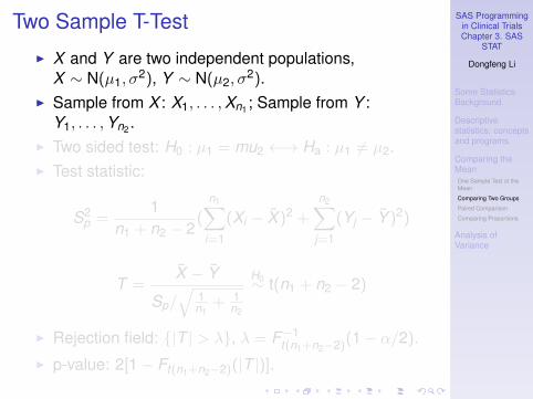
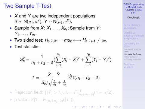

SAS Programmingin Clinical TrialsChapter 3. SAS
STAT
Dongfeng Li
Some StatisticsBackground
Descriptivestatistics: conceptsand programs
Comparing theMeanOne Sample Test of theMean
Comparing Two Groups
Paired Comparison
Comparing Proportions
Analysis ofVariance
One-sided Two-sample T-Test
I H0 : µ1 ≤ µ2 ←→ Ha : µ1 > µ2.I Rejection field: {T > λ}, λ = F−1
t(n1+n2−2)(1− α).I p-value: 1− Ft(n1+n2−2)(T ).I Prerequesits for two-sample t-test:
I Independence;I Normality.I Variance equality(homogeneity);
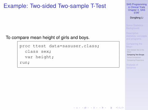
SAS Programmingin Clinical TrialsChapter 3. SAS
STAT
Dongfeng Li
Some StatisticsBackground
Descriptivestatistics: conceptsand programs
Comparing theMeanOne Sample Test of theMean
Comparing Two Groups
Paired Comparison
Comparing Proportions
Analysis ofVariance
Example: Two-sided Two-sample T-Test
To compare mean height of girls and boys.
proc ttest data=sasuser.class;class sex;var height;
run;

SAS Programmingin Clinical TrialsChapter 3. SAS
STAT
Dongfeng Li
Some StatisticsBackground
Descriptivestatistics: conceptsand programs
Comparing theMeanOne Sample Test of theMean
Comparing Two Groups
Paired Comparison
Comparing Proportions
Analysis ofVariance
Statistics
Variable sex N LowerCLMean
Mean UpperCLMean
LowerCLStdDev
Std Dev UpperCLStdDev
Std Err Min. Max.
height F 9 56.731 60.589 64.446 3.3897 5.0183 9.614 1.6728 51.3 66.5
height M 10 60.378 63.91 67.442 3.3965 4.9379 9.0147 1.5615 57.3 72
height Diff(1-2)
-8.145 -3.321 1.5025 3.7339 4.9759 7.4596 2.2863

SAS Programmingin Clinical TrialsChapter 3. SAS
STAT
Dongfeng Li
Some StatisticsBackground
Descriptivestatistics: conceptsand programs
Comparing theMeanOne Sample Test of theMean
Comparing Two Groups
Paired Comparison
Comparing Proportions
Analysis ofVariance
T-Tests
Variable Method Variances DF t Value Pr > |t|
height Pooled Equal 17 -1.45 0.1645
height Satterthwaite Unequal 16.7 -1.45 0.1652
Equality of Variances
Variable Method Num DF Den DF F Value Pr > F
height Folded F 8 9 1.03 0.9527

SAS Programmingin Clinical TrialsChapter 3. SAS
STAT
Dongfeng Li
Some StatisticsBackground
Descriptivestatistics: conceptsand programs
Comparing theMeanOne Sample Test of theMean
Comparing Two Groups
Paired Comparison
Comparing Proportions
Analysis ofVariance
I Female mean height 60.598, male mean height63.91.
I Two-sided t-test p-value=0.1652. No significantdifference between height of the two groups.
I Equal variance? There is a table for equality ofvariance test. P-value 0.9527 means that we canassume the two group have equal variance.
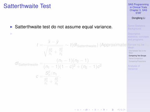
SAS Programmingin Clinical TrialsChapter 3. SAS
STAT
Dongfeng Li
Some StatisticsBackground
Descriptivestatistics: conceptsand programs
Comparing theMeanOne Sample Test of theMean
Comparing Two Groups
Paired Comparison
Comparing Proportions
Analysis ofVariance
Satterthwaite Test
I Satterthwaite test do not assume equal variance.I
t =x − y√S2
xn1
+S2
yn2
∼ t(dfSatterthwaite) (Approximately, under H0).
dfSatterthwaite =(n1 − 1)(n2 − 1)
(n1 − 1)(1− c)2 + (n2 − 1)c2
c =S2
x/n1
S2x
n1+
S2y
n2
.

SAS Programmingin Clinical TrialsChapter 3. SAS
STAT
Dongfeng Li
Some StatisticsBackground
Descriptivestatistics: conceptsand programs
Comparing theMeanOne Sample Test of theMean
Comparing Two Groups
Paired Comparison
Comparing Proportions
Analysis ofVariance
One-sided Two-sample T-test
I Ha should be sensible. If not, just accept H0.I Now that female mean height is 60.598, male mean
height 63.91, we could only test if male meanheight(denote µM) is higher than female meanheight(denote µF):
H0 : µF ≥ µM ←→ Ha : µF < µM
I P-value is half the two-sided p-value,0.1652/2 = 0.0826. Male height is not significantlyhigher than female height at significance level 0.05.

SAS Programmingin Clinical TrialsChapter 3. SAS
STAT
Dongfeng Li
Some StatisticsBackground
Descriptivestatistics: conceptsand programs
Comparing theMeanOne Sample Test of theMean
Comparing Two Groups
Paired Comparison
Comparing Proportions
Analysis ofVariance
Wilcoxon Rank Sum Test
I What if the two populations are not normal? Use thenonparametric Wilcoxon rank sum test.
I Rank: just like the ranks of grade scores, but rank 1corresponds the smallest value.
I Compare the mean rank of two independent groupsto see which group has higher value.

SAS Programmingin Clinical TrialsChapter 3. SAS
STAT
Dongfeng Li
Some StatisticsBackground
Descriptivestatistics: conceptsand programs
Comparing theMeanOne Sample Test of theMean
Comparing Two Groups
Paired Comparison
Comparing Proportions
Analysis ofVariance
Example: Two-sided Two-sample T-Test
Compare the GPA score of boys and girls.
proc npar1way data=sasuser.gpawilcoxon;
class sex;var gpa;
run;

SAS Programmingin Clinical TrialsChapter 3. SAS
STAT
Dongfeng Li
Some StatisticsBackground
Descriptivestatistics: conceptsand programs
Comparing theMeanOne Sample Test of theMean
Comparing Two Groups
Paired Comparison
Comparing Proportions
Analysis ofVariance
Wilcoxon Scores (Rank Sums) for Variable gpaClassified by Variable sex
sex N Sum ofScores
ExpectedUnderH0
Std DevUnderH0
MeanScore
female 145 16067.50 16312.50 463.429146 110.810345
male 79 9132.50 8887.50 463.429146 115.601266
Average scores were used for ties.

SAS Programmingin Clinical TrialsChapter 3. SAS
STAT
Dongfeng Li
Some StatisticsBackground
Descriptivestatistics: conceptsand programs
Comparing theMeanOne Sample Test of theMean
Comparing Two Groups
Paired Comparison
Comparing Proportions
Analysis ofVariance
Wilcoxon Two-Sample Test
Statistic 9132.5000
Normal Approximation
Z 0.5276
One-Sided Pr > Z 0.2989
Two-Sided Pr > |Z| 0.5978
t Approximation
One-Sided Pr > Z 0.2992
Two-Sided Pr > |Z| 0.5983
Z includes a continuity correction of 0.5.

SAS Programmingin Clinical TrialsChapter 3. SAS
STAT
Dongfeng Li
Some StatisticsBackground
Descriptivestatistics: conceptsand programs
Comparing theMeanOne Sample Test of theMean
Comparing Two Groups
Paired Comparison
Comparing Proportions
Analysis ofVariance
I Female mean score 110.8, male mean score 115.6,male scores better. Is it significant?
I For two-sided test, using normal approximation forthe test statistic, p-value is 0.5978, no significantdifference between the GPA scores of female andmale students.
I For one sided test, we can only test Ha : male scoresbetter. P-value is 0.2989, male is not significantlybetter than female regarding GPA scores.

SAS Programmingin Clinical TrialsChapter 3. SAS
STAT
Dongfeng Li
Some StatisticsBackground
Descriptivestatistics: conceptsand programs
Comparing theMeanOne Sample Test of theMean
Comparing Two Groups
Paired Comparison
Comparing Proportions
Analysis ofVariance
Paired Comparison
I Comparing two measurements of the same subject,instead of comparing the same measurement of twogroups of subjects, is a different problem fromtwo-sample test. It is called paired-comparison, weuse paired t-test to solve the problem.
I Example: Comparing the blood pressure of the samesubject before and after treatment by some drugs; ina fitness program, comparing the heart rate atentrance and at end of the program, etc.

SAS Programmingin Clinical TrialsChapter 3. SAS
STAT
Dongfeng Li
Some StatisticsBackground
Descriptivestatistics: conceptsand programs
Comparing theMeanOne Sample Test of theMean
Comparing Two Groups
Paired Comparison
Comparing Proportions
Analysis ofVariance
Paired T-test
I Let X be the “before” measurement, Y be the “after”measurement, both belong to the same subject, tocompare the mean of X and Y , let Z = X − Y , wesimply compare µZ with 0.
I Program solution 1: use PROC TTEST with PAIREDstatement. Need Z normal assumption.
I Program solution 2: first compute Z , then do onesample test H0 : µZ = 0←→ Ha : µZ 6= 0 usingPROC UNIVARIATE. This could also give the signedrank test and the sign test.
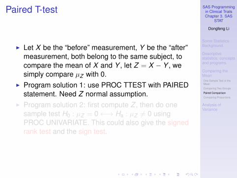

SAS Programmingin Clinical TrialsChapter 3. SAS
STAT
Dongfeng Li
Some StatisticsBackground
Descriptivestatistics: conceptsand programs
Comparing theMeanOne Sample Test of theMean
Comparing Two Groups
Paired Comparison
Comparing Proportions
Analysis ofVariance
Example: Paired T-Test Using PROC TTESTA stimulus is being examined to determine its effect onsystolic blood pressure. Twelve men participate in thestudy. Their systolic blood pressure is measured bothbefore and after the stimulus is applied. Program:
title ’Paired Comparison’;data pressure;
input SBPbefore SBPafter @@;datalines;
120 128 124 131 130 131 118 127140 132 128 125 140 141 135 137126 118 130 132 126 129 127 135;run;proc ttest;
paired SBPbefore*SBPafter;run;
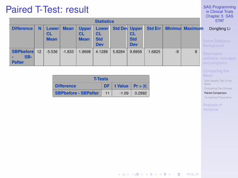
SAS Programmingin Clinical TrialsChapter 3. SAS
STAT
Dongfeng Li
Some StatisticsBackground
Descriptivestatistics: conceptsand programs
Comparing theMeanOne Sample Test of theMean
Comparing Two Groups
Paired Comparison
Comparing Proportions
Analysis ofVariance
Paired T-Test: resultStatistics
Difference N LowerCLMean
Mean UpperCLMean
LowerCLStdDev
Std Dev UpperCLStdDev
Std Err MinimumMaximum
SBPbefore- SB-Pafter
12 -5.536 -1.833 1.8698 4.1288 5.8284 9.8958 1.6825 -9 8
T-Tests
Difference DF t Value Pr > |t|
SBPbefore - SBPafter 11 -1.09 0.2992
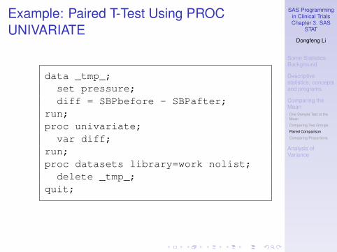
SAS Programmingin Clinical TrialsChapter 3. SAS
STAT
Dongfeng Li
Some StatisticsBackground
Descriptivestatistics: conceptsand programs
Comparing theMeanOne Sample Test of theMean
Comparing Two Groups
Paired Comparison
Comparing Proportions
Analysis ofVariance
Example: Paired T-Test Using PROCUNIVARIATE
data _tmp_;set pressure;diff = SBPbefore - SBPafter;
run;proc univariate;
var diff;run;proc datasets library=work nolist;
delete _tmp_;quit;
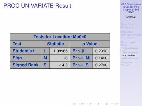
SAS Programmingin Clinical TrialsChapter 3. SAS
STAT
Dongfeng Li
Some StatisticsBackground
Descriptivestatistics: conceptsand programs
Comparing theMeanOne Sample Test of theMean
Comparing Two Groups
Paired Comparison
Comparing Proportions
Analysis ofVariance
PROC UNIVARIATE Result
Tests for Location: Mu0=0
Test Statistic p Value
Student’s t t -1.08965 Pr > |t| 0.2992
Sign M -3 Pr >= |M| 0.1460
Signed Rank S -14.5 Pr >= |S| 0.2700
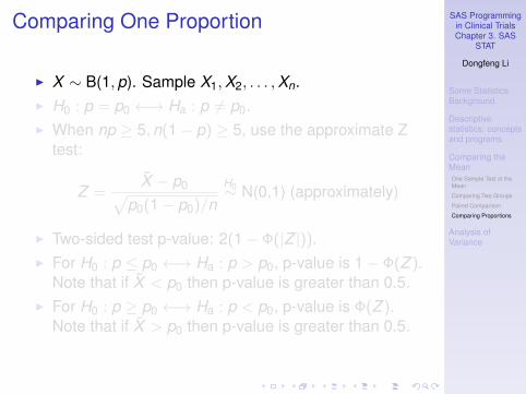
SAS Programmingin Clinical TrialsChapter 3. SAS
STAT
Dongfeng Li
Some StatisticsBackground
Descriptivestatistics: conceptsand programs
Comparing theMeanOne Sample Test of theMean
Comparing Two Groups
Paired Comparison
Comparing Proportions
Analysis ofVariance
Comparing One Proportion
I X ∼ B(1,p). Sample X1,X2, . . . ,Xn.I H0 : p = p0 ←→ Ha : p 6= p0.I When np ≥ 5,n(1− p) ≥ 5, use the approximate Z
test:
Z =X − p0√
p0(1− p0)/nH0∼ N(0,1) (approximately)
I Two-sided test p-value: 2(1− Φ(|Z |)).I For H0 : p ≤ p0 ←→ Ha : p > p0, p-value is 1− Φ(Z ).
Note that if X < p0 then p-value is greater than 0.5.I For H0 : p ≥ p0 ←→ Ha : p < p0, p-value is Φ(Z ).
Note that if X > p0 then p-value is greater than 0.5.

SAS Programmingin Clinical TrialsChapter 3. SAS
STAT
Dongfeng Li
Some StatisticsBackground
Descriptivestatistics: conceptsand programs
Comparing theMeanOne Sample Test of theMean
Comparing Two Groups
Paired Comparison
Comparing Proportions
Analysis ofVariance
Example: Heptitis B PercentI Is China’s heptitis B infected percent 8%?I A random sample of 100 persons show 5 infected with
heptitis B.
%MACRO percentzt(n,n1,p0);data _null_;
file print;p0 = &p0.; n = &n.; n1 = &n1.;xbar = n1/n;Z = (xbar - p0)/sqrt(p0 * (1-p0)/n);ptwosided = 2*(1 - probnorm(abs(Z)));prightsided = 1 - probnorm(Z);pleftsided = probnorm(Z);put ’===== Test for percent =====’;put ’n = ’ n ’ p =’ xbar;put ’p0 = ’ p0;put ’Z = ’ Z;put ’Pr > |Z|: ’ ptwosided pvalue.;put ’Pr > Z: ’ prightsided pvalue.;put ’Pr < Z: ’ pleftsided pvalue.;
run;%MEND percentzt;%percentzt(100,5,0.08);
I Conclusion: no significant difference with 8%.

SAS Programmingin Clinical TrialsChapter 3. SAS
STAT
Dongfeng Li
Some StatisticsBackground
Descriptivestatistics: conceptsand programs
Comparing theMeanOne Sample Test of theMean
Comparing Two Groups
Paired Comparison
Comparing Proportions
Analysis ofVariance
Comparing Two Propotions–Two-Sided
I X ∼ B(1,p1), Y ∼ B(1,p2), independent, testH0 : p1 = p2 ←→ Ha : p1 6= p2.
I n1 trials of X gives s1 successes, n2 trials of Y givess2 successes.
I When n1 and n2 large, let W = s1n1− s2
n2, then
SE2(W ) ≈ p(1− p)(
1n1
+ 1n2
), W/SE(W ) is
asymptotically distributed N(0,1). p = s1+s2n1+n2
.I Let Z = W/SE(W ), p-value is 2(1− Φ(|Z |)).

SAS Programmingin Clinical TrialsChapter 3. SAS
STAT
Dongfeng Li
Some StatisticsBackground
Descriptivestatistics: conceptsand programs
Comparing theMeanOne Sample Test of theMean
Comparing Two Groups
Paired Comparison
Comparing Proportions
Analysis ofVariance
Comparing Two Propotions–One-Sided
I When n1 and n2 large, let W = p1 − p2, thenSE2(W ) ≈ p1(1−p1)
n1+ p2(1−p2)
n2, W/SE(W ) is
asymptotically distributed N(0,1) when p1 = p2.p1 = s1
n1, p2 = s2
n2.
I Let Z = W/SE(W ).I For right-sided alternative, p-value is 1− Φ(Z ).I For left-sided alternative, p-value is Φ(Z ).

SAS Programmingin Clinical TrialsChapter 3. SAS
STAT
Dongfeng Li
Some StatisticsBackground
Descriptivestatistics: conceptsand programs
Comparing theMeanOne Sample Test of theMean
Comparing Two Groups
Paired Comparison
Comparing Proportions
Analysis ofVariance
Example: Heptitis B Proportions of Male andFemale
I Do male and female have the same proportion ofHepatitis B infected?
I A random sample of 100 males, 100 females show10 males infected with heptitis B, 8 females infected.
I Test result:
Pr > |Z | : 0.6212Pr > Z : 0.3105Pr < Z : 0.6895
I Conclusion: no significant difference between maleand female.
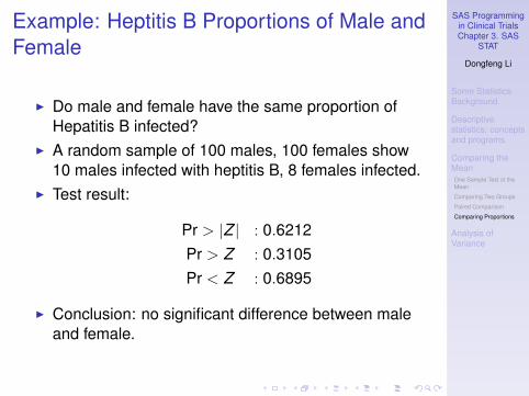

SAS Programmingin Clinical TrialsChapter 3. SAS
STAT
Dongfeng Li
Some StatisticsBackground
Descriptivestatistics: conceptsand programs
Comparing theMeanOne Sample Test of theMean
Comparing Two Groups
Paired Comparison
Comparing Proportions
Analysis ofVariance
%MACRO percent2z(n1,s1,n2,s2);data _null_;
file print;n1=&n1; s1=&s1; n2=&n2; s2=&s2;hatp = (s1+s2)/(n1+n2);hatp1 = s1/n1; hatp2 = s2/n2;Z2s = (hatp1 - hatp2) /
sqrt(hatp*(1-hatp)*(1/n1 + 1/n2));Z1s = (hatp1 - hatp2) /
sqrt(hatp1*(1-hatp1)/n1+hatp2*(1-hatp2)/n2);
ptwosided = 2*(1 - probnorm(abs(Z2s)));prightsided = 1 - probnorm(Z1s);pleftsided = probnorm(Z1s);put ’===== Test for percent =====’;put ’n1 = ’ n1 ’ s1 =’ s1 ’ p1=’ hatp1;put ’n2 = ’ n2 ’ s2 =’ s2 ’ p2=’ hatp2;put ’Pr > |Z|: ’ ptwosided pvalue.;put ’Pr > Z: ’ prightsided pvalue.;put ’Pr < Z: ’ pleftsided pvalue.;
run;%MEND percent2z;%percent2z(100,10,100,8);

SAS Programmingin Clinical TrialsChapter 3. SAS
STAT
Dongfeng Li
Some StatisticsBackground
Descriptivestatistics: conceptsand programs
Comparing theMean
Analysis ofVarianceOne-Way ANOVA
Two-Way ANOVA
Analysis of Variance
I Test for significant effect of some factors on aresponse.
I One-way ANOVA.I Nonparametric Kruskal-Wallis test.I Two-way ANOVA, additive models, interactions.

SAS Programmingin Clinical TrialsChapter 3. SAS
STAT
Dongfeng Li
Some StatisticsBackground
Descriptivestatistics: conceptsand programs
Comparing theMean
Analysis ofVarianceOne-Way ANOVA
Two-Way ANOVA
One-Way ANOVA
I Two sample t-test −→ one-way anova:I Response Y , group C(factor).I Two sample t-test: Compare the mean of Y in the
two groups of C.I One-way ANOVA: Compare the mean of Y in more
than two groups of C.I Question:
I Is there any significant difference among the meansof Y of different groups? Equvalently, does factor Chave significant effect on the mean level of Y?
I Which pair of groups have significant meandifference? This is the multiple comparison problem.
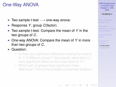

SAS Programmingin Clinical TrialsChapter 3. SAS
STAT
Dongfeng Li
Some StatisticsBackground
Descriptivestatistics: conceptsand programs
Comparing theMean
Analysis ofVarianceOne-Way ANOVA
Two-Way ANOVA
Example: The Comparison of Veneer BrandsI Compare WEAR of 5 BRANDS. Each brand has 4
samples.I Use PROC ANOVA or PROC GLM. PROC GLM
should be used for unbalanced design.I Theoretical prerequesits: Independence, normal
distribution, equal variances.I Data:
data veneer;input brand $ wear @@;datalines;
ACME 2.3 ACME 2.1 ACME 2.4 ACME 2.5CHAMP 2.2 CHAMP 2.3 CHAMP 2.4 CHAMP 2.6AJAX 2.2 AJAX 2.0 AJAX 1.9 AJAX 2.1TUFFY 2.4 TUFFY 2.7 TUFFY 2.6 TUFFY 2.7XTRA 2.3 XTRA 2.5 XTRA 2.3 XTRA 2.4;run;

SAS Programmingin Clinical TrialsChapter 3. SAS
STAT
Dongfeng Li
Some StatisticsBackground
Descriptivestatistics: conceptsand programs
Comparing theMean
Analysis ofVarianceOne-Way ANOVA
Two-Way ANOVA
I Example using PROC ANOVA:
proc anova data=veneer;class brand;model wear = brand;
quit;
I Example using PROC GLM:
proc glm data=samp.veneer;class brand;model wear = brand;
quit;
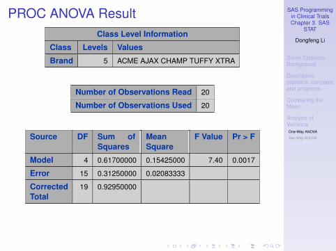
SAS Programmingin Clinical TrialsChapter 3. SAS
STAT
Dongfeng Li
Some StatisticsBackground
Descriptivestatistics: conceptsand programs
Comparing theMean
Analysis ofVarianceOne-Way ANOVA
Two-Way ANOVA
PROC ANOVA ResultClass Level Information
Class Levels Values
Brand 5 ACME AJAX CHAMP TUFFY XTRA
Number of Observations Read 20
Number of Observations Used 20
Source DF Sum ofSquares
MeanSquare
F Value Pr > F
Model 4 0.61700000 0.15425000 7.40 0.0017
Error 15 0.31250000 0.02083333
CorrectedTotal
19 0.92950000

SAS Programmingin Clinical TrialsChapter 3. SAS
STAT
Dongfeng Li
Some StatisticsBackground
Descriptivestatistics: conceptsand programs
Comparing theMean
Analysis ofVarianceOne-Way ANOVA
Two-Way ANOVA
R-Square Coeff Var Root MSE Wear Mean
0.663798 6.155120 0.144338 2.345000
Source DF Anova SS Mean Square F Value Pr > F
Brand 4 0.61700000 0.15425000 7.40 0.0017

SAS Programmingin Clinical TrialsChapter 3. SAS
STAT
Dongfeng Li
Some StatisticsBackground
Descriptivestatistics: conceptsand programs
Comparing theMean
Analysis ofVarianceOne-Way ANOVA
Two-Way ANOVA
PROC GLM ResultThe data information, model analysis of variance, model fit statistics partare very similar to PROC ANOVA results.Different results:
Source DF Type I SS Mean Square F Value Pr > F
Brand 4 0.61700000 0.15425000 7.40 0.0017
Source DF Type III SS Mean Square F Value Pr > F
Brand 4 0.61700000 0.15425000 7.40 0.0017

SAS Programmingin Clinical TrialsChapter 3. SAS
STAT
Dongfeng Li
Some StatisticsBackground
Descriptivestatistics: conceptsand programs
Comparing theMean
Analysis ofVarianceOne-Way ANOVA
Two-Way ANOVA
Multiple Comparison
I Two test which pairs have significant differences,which are not significantly different.
I For 5 groups, we have(5
2
)= 10 pairs to compare.
I Two kinds of type I errors:I Comparisonwise error rate(CER), only controls the
type I error rate of each comparison;I Experimentwise error rate(FWR, Familywide Error
Rate), controls the type I error rate of all of thecomparisons.
I Controling experimental error rate is more cautious.I Control CER to discovery more possible differences.I Control FWR to make sound inference.

SAS Programmingin Clinical TrialsChapter 3. SAS
STAT
Dongfeng Li
Some StatisticsBackground
Descriptivestatistics: conceptsand programs
Comparing theMean
Analysis ofVarianceOne-Way ANOVA
Two-Way ANOVA
Fisher’s Least Significant Difference Test
I Fisher’s LSD test controls the comparison error rate.I Like repeated two-sample tests, but use a common
SE estimate of the numerator.I Let yij be the observation of j ’th individual of the i ’th
category, j = 1, . . . , r , i = 1, . . . ,g. yi· is the samplemean of the i ’th group.
I Let
SE2(yi· − yk ·) ≡1
g(r − 1)
∑i
∑j
(yij − yi·)2
I
Tik =yi· − yk ·
SE(yi· − yk ·)
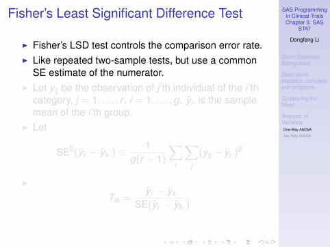

SAS Programmingin Clinical TrialsChapter 3. SAS
STAT
Dongfeng Li
Some StatisticsBackground
Descriptivestatistics: conceptsand programs
Comparing theMean
Analysis ofVarianceOne-Way ANOVA
Two-Way ANOVA
Example of Fisher’s LSD Testproc anova data=samp.veneer;
class brand;model wear = brand;means brand / t;
quit;
t Tests (LSD) for Wear
Note This test controls the Type I comparisonwise error rate, not theexperimentwise error rate.
Alpha 0.05
Error Degrees of Freedom 15
Error Mean Square 0.020833
Critical Value of t 2.13145
Least Significant Difference 0.2175
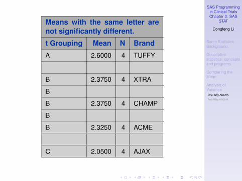
SAS Programmingin Clinical TrialsChapter 3. SAS
STAT
Dongfeng Li
Some StatisticsBackground
Descriptivestatistics: conceptsand programs
Comparing theMean
Analysis ofVarianceOne-Way ANOVA
Two-Way ANOVA
Means with the same letter arenot significantly different.
t Grouping Mean N Brand
A 2.6000 4 TUFFY
B 2.3750 4 XTRA
B
B 2.3750 4 CHAMP
B
B 2.3250 4 ACME
C 2.0500 4 AJAX

SAS Programmingin Clinical TrialsChapter 3. SAS
STAT
Dongfeng Li
Some StatisticsBackground
Descriptivestatistics: conceptsand programs
Comparing theMean
Analysis ofVarianceOne-Way ANOVA
Two-Way ANOVA
REGWQ Test
I REGWQ test is one of the multiple testing methodswhich controls the experiment wise type I error rate.
I Example:
proc anova data=samp.veneer;class brand;model wear = brand;means brand / regwq;
quit;
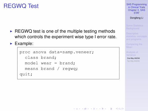
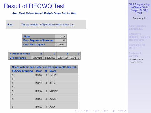
SAS Programmingin Clinical TrialsChapter 3. SAS
STAT
Dongfeng Li
Some StatisticsBackground
Descriptivestatistics: conceptsand programs
Comparing theMean
Analysis ofVarianceOne-Way ANOVA
Two-Way ANOVA
Result of REGWQ TestRyan-Einot-Gabriel-Welsch Multiple Range Test for Wear
Note This test controls the Type I experimentwise error rate.
Alpha 0.05
Error Degrees of Freedom 15
Error Mean Square 0.020833
Number of Means 2 3 4 5
Critical Range 0.264828 0.2917322 0.2941581 0.31516
Means with the same letter are not significantly different.
REGWQ Grouping Mean N Brand
A 2.6000 4 TUFFY
A
A 2.3750 4 XTRA
A
A 2.3750 4 CHAMP
A
A 2.3250 4 ACME
B 2.0500 4 AJAX

SAS Programmingin Clinical TrialsChapter 3. SAS
STAT
Dongfeng Li
Some StatisticsBackground
Descriptivestatistics: conceptsand programs
Comparing theMean
Analysis ofVarianceOne-Way ANOVA
Two-Way ANOVA
The Kruskal-Wallis Test
I What if the samples are not normally ditributed? Usethe nonparametric Kruskal-Wallis test, similar to theWilcoxon rank sum test.
I Compute ranks of Y observations. Compare themean rank of the groups.
I Use PROC NPAR1WAY with the WILCOXON option.

SAS Programmingin Clinical TrialsChapter 3. SAS
STAT
Dongfeng Li
Some StatisticsBackground
Descriptivestatistics: conceptsand programs
Comparing theMean
Analysis ofVarianceOne-Way ANOVA
Two-Way ANOVA
Example: Kruskal-Wallis Test
I Compare wear of different brands.I Code:
proc npar1way data=samp.veneer wilcoxon;class brand;var wear;

SAS Programmingin Clinical TrialsChapter 3. SAS
STAT
Dongfeng Li
Some StatisticsBackground
Descriptivestatistics: conceptsand programs
Comparing theMean
Analysis ofVarianceOne-Way ANOVA
Two-Way ANOVA
Result of Kruskal-Wallis TestWilcoxon Scores (Rank Sums) for VariableWearClassified by Variable Brand
Brand N Sum ofScores
ExpectedUnderH0
Std DevUnderH0
MeanScore
ACME 4 40.0 42.0 10.483069 10.000
CHAMP 4 44.0 42.0 10.483069 11.000
AJAX 4 12.0 42.0 10.483069 3.000
TUFFY 4 69.0 42.0 10.483069 17.250
XTRA 4 45.0 42.0 10.483069 11.250
Average scores were used for ties.
Kruskal-Wallis Test
Chi-Square 11.9824
DF 4
Pr > Chi-Square 0.0175

SAS Programmingin Clinical TrialsChapter 3. SAS
STAT
Dongfeng Li
Some StatisticsBackground
Descriptivestatistics: conceptsand programs
Comparing theMean
Analysis ofVarianceOne-Way ANOVA
Two-Way ANOVA
Two-Way ANOVA—Main Effects
I Consider the simple case of balanced completedesign of two factors, with repetition.
I Main effects model(additive model)
yijk =µ+ αi + βj + eijk
i = 1, . . . ,n, j = 1, . . . ,m, k = 1, . . . , r(r ≥ 1)
I yijk is the response of factor A at level i , factor B atlevel j , repetition k .
I µ is the over all average.I αi is the main effect of factor A at level i .
∑i αi = 0.
I βj is the main effect of factor B at level j .∑
j βj = 0.I eijk i.i.d. N(0, σ2).

SAS Programmingin Clinical TrialsChapter 3. SAS
STAT
Dongfeng Li
Some StatisticsBackground
Descriptivestatistics: conceptsand programs
Comparing theMean
Analysis ofVarianceOne-Way ANOVA
Two-Way ANOVA
Two-Way ANOVA—Interactions
I Interaction effect model
yijk =µ+ αi + βj + γi,j + eijk
i = 1, . . . ,n, j = 1, . . . ,m, k = 1, . . . , r(r ≥ 2)
I γi,j is called an interaction effect.∑i γi,j = 0,
∑j γi,j = 0.
I Use PROC ANOVA or PROC GLM. For unbalanceddesign, use PROC GLM.

SAS Programmingin Clinical TrialsChapter 3. SAS
STAT
Dongfeng Li
Some StatisticsBackground
Descriptivestatistics: conceptsand programs
Comparing theMean
Analysis ofVarianceOne-Way ANOVA
Two-Way ANOVA
Example of InteractionsI Example with only main effects: n = m = 2, r ≥ 2, µ = 10,α1 = 4, α2 = −4, β1 = 2, β2 = −2. If interaction effect doesnot exist(γi,j ≡ 0), then
Ey11k =10 + 4 + 2 = 16Ey12k =10 + 4− 2 = 12Ey21k =10− 4 + 2 = 8Ey22k =10− 4− 2 = 4
I Example with interactions: Suppose γ1,1 = 1, thenγ1,2 = −1, γ2,1 = −1, γ2,2 = 1, so
Ey11k =16 + 1 = 17Ey12k =12− 1 = 11Ey21k =8− 1 = 7Ey22k =4 + 1 = 5
the interaction increases the expectation when A and B areboth 1 or both 2, decreases the expectation other wise.

SAS Programmingin Clinical TrialsChapter 3. SAS
STAT
Dongfeng Li
Some StatisticsBackground
Descriptivestatistics: conceptsand programs
Comparing theMean
Analysis ofVarianceOne-Way ANOVA
Two-Way ANOVA
Two-way ANOVA ExampleI To study the effects of different production factors on
the strenth of some rubber product, consider 3 levelsof factor A, 4 levels of factor B, completeexperiement with 3× 4 = 12 combinations, eachrepeated 2 times, so we have n = 24 experiments.
I Data:data rubber;
do a=1 to 3; do b=1 to 4; do r=1 to 2;input stren @@;output;
end; end; end;cards;
31 33 34 36 35 36 39 3833 34 36 37 37 39 38 4135 37 37 38 39 40 42 44;run;

SAS Programmingin Clinical TrialsChapter 3. SAS
STAT
Dongfeng Li
Some StatisticsBackground
Descriptivestatistics: conceptsand programs
Comparing theMean
Analysis ofVarianceOne-Way ANOVA
Two-Way ANOVA
I Interaction model:
proc anova data=rubber;class a b;model stren = a b a*b;
run;
I Main effects(additive) model:
proc anova data=rubber;class a b;model stren = a b;
run;

SAS Programmingin Clinical TrialsChapter 3. SAS
STAT
Dongfeng Li
Some StatisticsBackground
Descriptivestatistics: conceptsand programs
Comparing theMean
Analysis ofVarianceOne-Way ANOVA
Two-Way ANOVA
Result
Class Level Information
Class Levels Values
a 3 1 2 3
b 4 1 2 3 4
Number of Observations Read 24
Number of Observations Used 24

SAS Programmingin Clinical TrialsChapter 3. SAS
STAT
Dongfeng Li
Some StatisticsBackground
Descriptivestatistics: conceptsand programs
Comparing theMean
Analysis ofVarianceOne-Way ANOVA
Two-Way ANOVA
Source DF SumofSquares
MeanSquare
F Value Pr > F
Model 11 193.4583333 17.5871212 12.06 <.0001
Error 12 17.5000000 1.4583333
CorrectedTotal
23 210.9583333
R-Square Coeff Var Root MSE stren Mean
0.917045 3.260152 1.207615 37.04167
Source DF Anova SS MeanSquare
F Value Pr > F
a 2 56.5833333 28.2916667 19.40 0.0002
b 3 132.1250000 44.0416667 30.20 <.0001
a*b 6 4.7500000 0.7916667 0.54 0.7665

SAS Programmingin Clinical TrialsChapter 3. SAS
STAT
Dongfeng Li
Some StatisticsBackground
Descriptivestatistics: conceptsand programs
Comparing theMean
Analysis ofVarianceOne-Way ANOVA
Two-Way ANOVA
Additive model result
Source DF Sum ofSquares
MeanSquare
F Value Pr > F
Model 5 188.7083333 37.7416667 30.53 <.0001
Error 18 22.2500000 1.2361111
CorrectedTotal
23 210.9583333
R-Square Coeff Var Root MSE stren Mean
0.894529 3.001499 1.111805 37.04167
Source DF Anova SS MeanSquare
F Value Pr > F
a 2 56.5833333 28.2916667 22.89 <.0001
b 3 132.1250000 44.0416667 35.63 <.0001