sanders/van stee: approximations- und online-algorithmen...
TRANSCRIPT
Sanders/van Stee: Approximations- und Online-Algorithmen 1
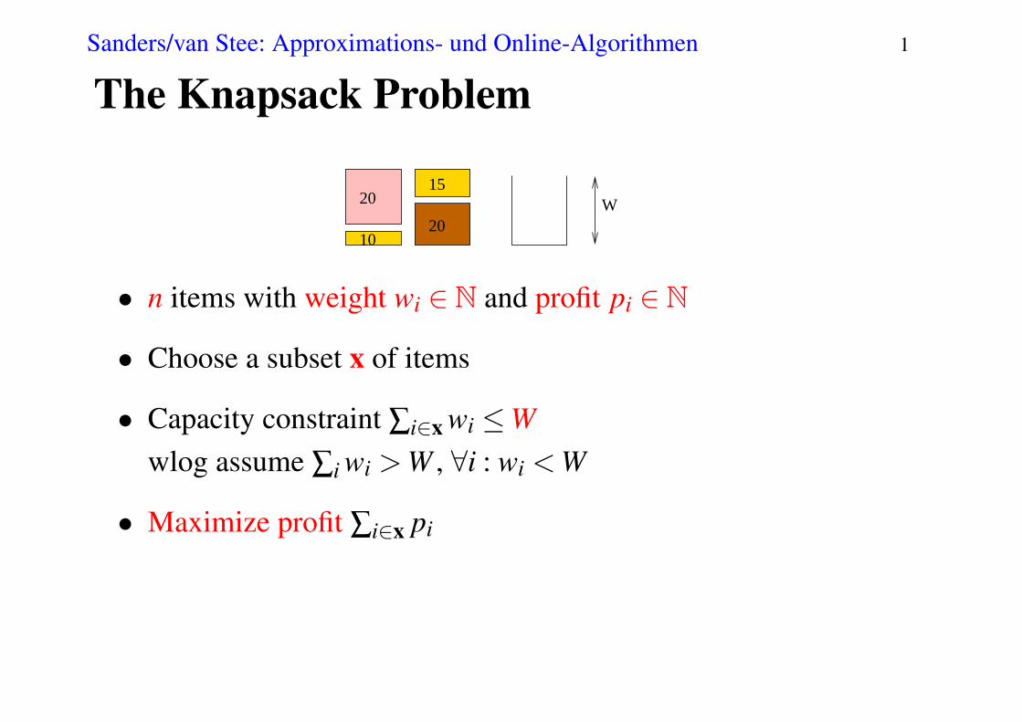
The Knapsack Problem
W20
1020
15
• n items with weight wi ∈ N and profit pi ∈ N• Choose a subset x of items
• Capacity constraint ∑i∈x wi ≤Wwlog assume ∑i wi > W , ∀i : wi < W
• Maximize profit ∑i∈x pi
Sanders/van Stee: Approximations- und Online-Algorithmen 2
Reminder?: Linear Programming
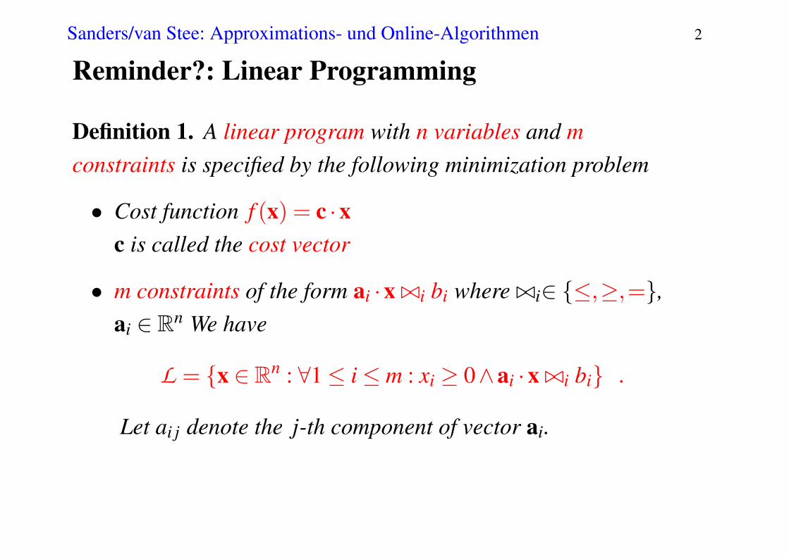
Definition 1. A linear program with n variables and mconstraints is specified by the following minimization problem
• Cost function f (x) = c ·xc is called the cost vector
• m constraints of the form ai ·x ./i bi where ./i∈ {≤,≥,=},ai ∈ Rn We have
L = {x ∈ Rn : ∀1≤ i≤ m : xi ≥ 0∧ai ·x ./i bi} .
Let ai j denote the j-th component of vector ai.
Sanders/van Stee: Approximations- und Online-Algorithmen 3
Complexity
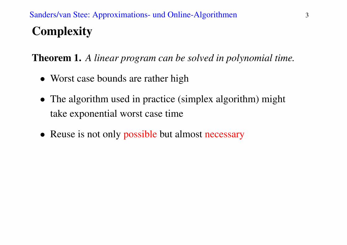
Theorem 1. A linear program can be solved in polynomial time.
• Worst case bounds are rather high
• The algorithm used in practice (simplex algorithm) mighttake exponential worst case time
• Reuse is not only possible but almost necessary

Sanders/van Stee: Approximations- und Online-Algorithmen 4
Integer Linear Programming
ILP: Integer Linear Program, A linear program with theadditional constraint that all the xi ∈ Z
Linear Relaxation: Remove the integrality constraints from anILP
Sanders/van Stee: Approximations- und Online-Algorithmen 5
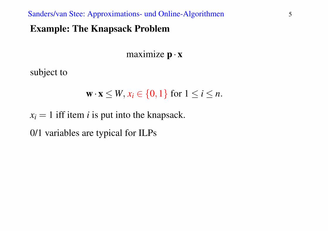
Example: The Knapsack Problem
maximize p ·xsubject to
w ·x≤W, xi ∈ {0,1} for 1≤ i≤ n.
xi = 1 iff item i is put into the knapsack.
0/1 variables are typical for ILPs

Sanders/van Stee: Approximations- und Online-Algorithmen 6
Linear relaxation for the knapsack problem
maximize p ·xsubject to
w ·x≤W, 0≤ xi ≤ 1 for 1≤ i≤ n.
We allow items to be picked “fractionally”
x1 = 1/3 means that 1/3 of item 1 is put into the knapsack
This makes the problem much easier. How would you solve it?

Sanders/van Stee: Approximations- und Online-Algorithmen 7
The Knapsack Problem
W20
1020
15
• n items with weight wi ∈ N and profit pi ∈ N• Choose a subset x of items
• Capacity constraint ∑i∈x wi ≤Wwlog assume ∑i wi > W , ∀i : wi < W
• Maximize profit ∑i∈x pi
Sanders/van Stee: Approximations- und Online-Algorithmen 8
How to Cope with ILPs
− Solving ILPs is NP-hard
+ Powerful modeling language
+ There are generic methods that sometimes work well
+ Many ways to get approximate solutions.
+ The solution of the integer relaxation helps. For examplesometimes we can simply round.

Sanders/van Stee: Approximations- und Online-Algorithmen 9
Linear Time Algorithm forLinear Relaxation of Knapsack
Classify elements by profit densitypi
wiinto B,{k},S such that
∀i ∈ B, j ∈ S :pi
wi≥ pk
wk≥ p j
w j, and,
∑i∈B
wi ≤W but wk + ∑i∈B
wi > W .
Set xi =
1 if i ∈ BW−∑i∈B wi
wkif i = k
0 if i ∈ S
1015
20
20
WB
S
k
Sanders/van Stee: Approximations- und Online-Algorithmen 10
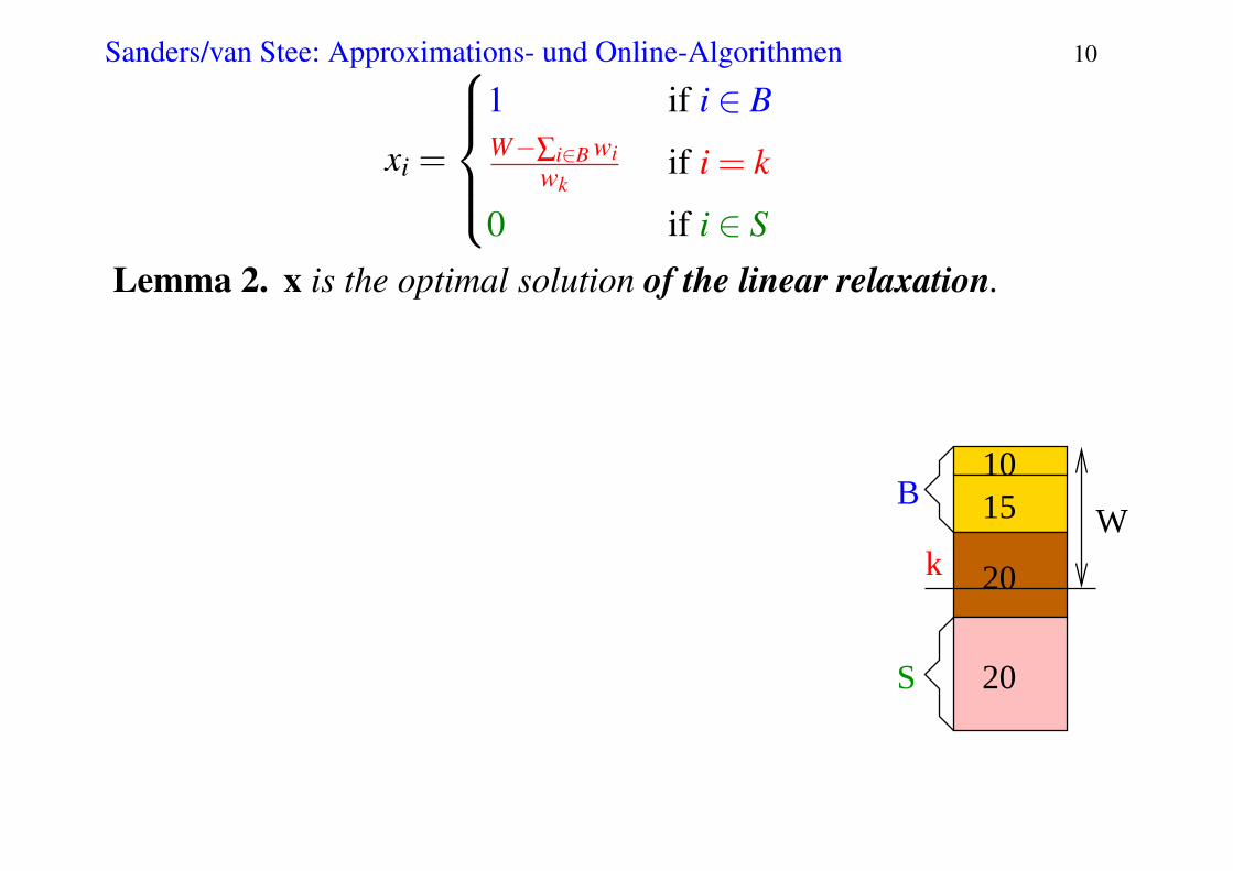
xi =
1 if i ∈ BW−∑i∈B wi
wkif i = k
0 if i ∈ S
Lemma 2. x is the optimal solution of the linear relaxation.
Proof. Let x∗ denote the optimal solution
• w ·x∗ = W otherwise increase some xi
• ∀i ∈ B : x∗i = 1 otherwiseincrease x∗i and decrease some x∗j for j ∈ {k}∪S
• ∀ j ∈ S : x∗j = 0 otherwisedecrease x∗j and increase x∗k
• This only leaves
1015
20
20
WB
S
k

Sanders/van Stee: Approximations- und Online-Algorithmen 11
xi =
1 if i ∈ BW−∑i∈B wi
wkif i = k
0 if i ∈ S
Lemma 2. x is the optimal solution of the linear relaxation.
Proof. Let x∗ denote the optimal solution
• w ·x∗ = W otherwise increase some xi
• ∀i ∈ B : x∗i = 1 otherwiseincrease x∗i and decrease some x∗j for j ∈ {k}∪S
• ∀ j ∈ S : x∗j = 0 otherwisedecrease x∗j and increase x∗k
• This only leaves
1015
20
20
WB
S
k
Sanders/van Stee: Approximations- und Online-Algorithmen 12
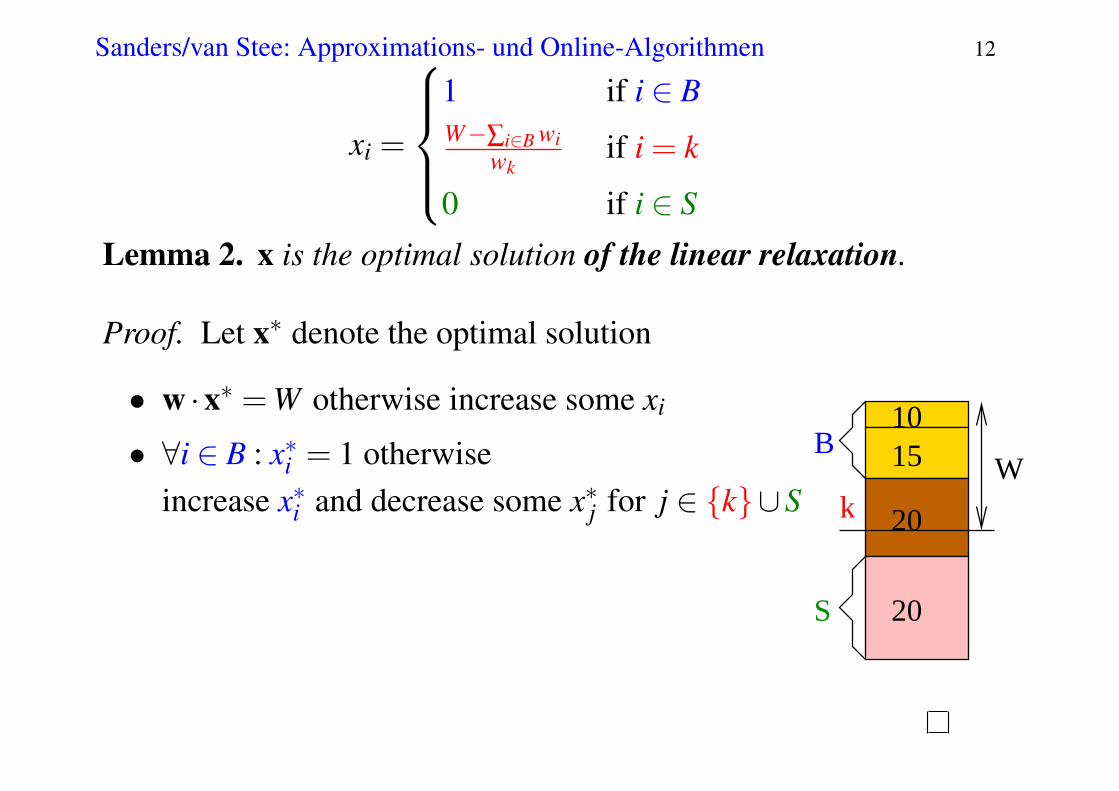
xi =
1 if i ∈ BW−∑i∈B wi
wkif i = k
0 if i ∈ S
Lemma 2. x is the optimal solution of the linear relaxation.
Proof. Let x∗ denote the optimal solution
• w ·x∗ = W otherwise increase some xi
• ∀i ∈ B : x∗i = 1 otherwiseincrease x∗i and decrease some x∗j for j ∈ {k}∪S
• ∀ j ∈ S : x∗j = 0 otherwisedecrease x∗j and increase x∗k
• This only leaves
1015
20
20
WB
S
k
Sanders/van Stee: Approximations- und Online-Algorithmen 13
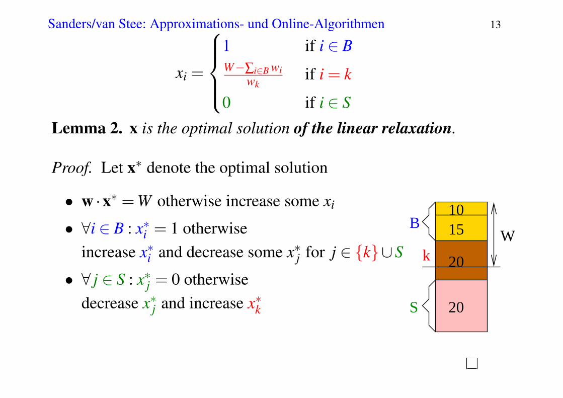
xi =
1 if i ∈ BW−∑i∈B wi
wkif i = k
0 if i ∈ S
Lemma 2. x is the optimal solution of the linear relaxation.
Proof. Let x∗ denote the optimal solution
• w ·x∗ = W otherwise increase some xi
• ∀i ∈ B : x∗i = 1 otherwiseincrease x∗i and decrease some x∗j for j ∈ {k}∪S
• ∀ j ∈ S : x∗j = 0 otherwisedecrease x∗j and increase x∗k
• This only leaves
1015
20
20
WB
S
k
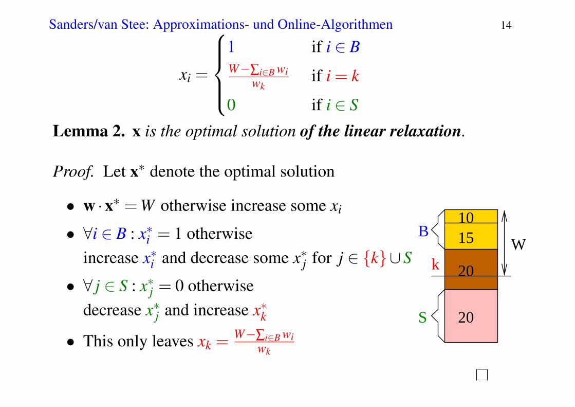
Sanders/van Stee: Approximations- und Online-Algorithmen 14
xi =
1 if i ∈ BW−∑i∈B wi
wkif i = k
0 if i ∈ S
Lemma 2. x is the optimal solution of the linear relaxation.
Proof. Let x∗ denote the optimal solution
• w ·x∗ = W otherwise increase some xi
• ∀i ∈ B : x∗i = 1 otherwiseincrease x∗i and decrease some x∗j for j ∈ {k}∪S
• ∀ j ∈ S : x∗j = 0 otherwisedecrease x∗j and increase x∗k
• This only leaves xk = W−∑i∈B wiwk
1015
20
20
WB
S
k

Sanders/van Stee: Approximations- und Online-Algorithmen 15
xi =
1 if i ∈ BW−∑i∈B wi
wkif i = k
0 if i ∈ S
Lemma 3. For the optimal solution x of the linear relaxation:
opt≤∑i
xi pi ≤ 2opt
Proof. We have∑i∈B pi ≤ opt. Furthermore, since wk < W ,pk ≤ opt.We get
opt≤∑i
xi pi ≤ ∑i∈B
pi + pk ≤ opt+opt = 2opt
1015
20
20
WB
S
k

Sanders/van Stee: Approximations- und Online-Algorithmen 16
Two-approximation of Knapsack
xi =
1 if i ∈ BW−∑i∈B wi
wkif i = k
0 if i ∈ S
Exercise: Prove that either B or {k} is a2-approximation of the (nonrelaxed) knapsack problem.
1015
20
20
WB
S
k

Sanders/van Stee: Approximations- und Online-Algorithmen 17
Dynamic Programming— Building it Piece By PiecePrinciple of Optimality
• An optimal solution can be viewed as constructed ofoptimal solutions for subproblems
• Solutions with the same objective values areinterchangeable
Example: Shortest Paths• Any subpath of a shortest path is a shortest path
• Shortest subpaths are interchangeable
s tu v

Sanders/van Stee: Approximations- und Online-Algorithmen 18
Dynamic Programming by Capacityfor the Knapsack Problem
DefineP(i,C) = optimal profit from items 1,. . . ,i using capacity ≤C.
Lemma 4.
∀1≤ i≤ n : P(i,C) = max(P(i−1,C),
P(i−1,C−wi)+ pi)

Sanders/van Stee: Approximations- und Online-Algorithmen 19
Lemma 4.∀1≤ i≤ n : P(i,C) = max(P(i−1,C), P(i−1,C−wi)+ pi)
ProofP(i,C)≥ P(i−1,C): Set xi = 0, use optimal subsolution.

Sanders/van Stee: Approximations- und Online-Algorithmen 20
Lemma 4.∀1≤ i≤ n : P(i,C) = max(P(i−1,C), P(i−1,C−wi)+ pi)
ProofP(i,C)≥ P(i−1,C): Set xi = 0, use optimal subsolution.
P(i,C)≥ P(i−1,C−wi)+ pi: Set xi = 1 . . .
Therefore P(i,C)≥max(P(i−1,C), P(i−1,C−wi)+ pi).

Sanders/van Stee: Approximations- und Online-Algorithmen 21
Lemma 4.∀1≤ i≤ n : P(i,C) = max(P(i−1,C), P(i−1,C−wi)+ pi)
ProofP(i,C)≤max(P(i−1,C),P(i−1,C−wi)+ pi).
Assume the contrary :∃x that is optimal for the subproblem such that
P(i−1,C) < p ·x ∧ P(i−1,C−wi)+ pi < p ·x

Sanders/van Stee: Approximations- und Online-Algorithmen 22
Lemma 4.∀1≤ i≤ n : P(i,C) = max(P(i−1,C), P(i−1,C−wi)+ pi)
ProofP(i,C)≤max(P(i−1,C),P(i−1,C−wi)+ pi)
Assume the contrary :∃x that is optimal for the subproblem such that
P(i−1,C) < p ·x ∧ P(i−1,C−wi)+ pi < p ·xCase xi = 0: x is also feasible for P(i−1,C). Hence,
P(i−1,C)≥ p ·x. Contradiction
Sanders/van Stee: Approximations- und Online-Algorithmen 23
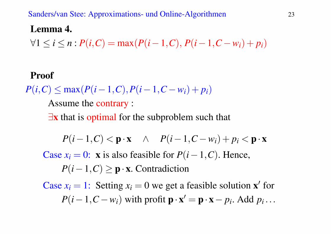
Lemma 4.∀1≤ i≤ n : P(i,C) = max(P(i−1,C), P(i−1,C−wi)+ pi)
ProofP(i,C)≤max(P(i−1,C),P(i−1,C−wi)+ pi)
Assume the contrary :∃x that is optimal for the subproblem such that
P(i−1,C) < p ·x ∧ P(i−1,C−wi)+ pi < p ·xCase xi = 0: x is also feasible for P(i−1,C). Hence,
P(i−1,C)≥ p ·x. Contradiction
Case xi = 1: Setting xi = 0 we get a feasible solution x′ forP(i−1,C−wi) with profit p ·x′ = p ·x− pi. Add pi . . .

Sanders/van Stee: Approximations- und Online-Algorithmen 24
Computing P(i,C) bottom up:
Procedure knapsack(p, c, n, W )array P[0 . . .W ] = [0, . . . ,0]bitarray decision[1 . . .n,0 . . .W ] = [(0, . . . ,0), . . . ,(0, . . . ,0)]for i := 1 to n do
// invariant: ∀C ∈ {1, . . . ,W} : P[C] = P(i−1,C)for C := W downto wi do
if P[C−wi]+ pi > P[C] thenP[C] := P[C−wi]+ pi
decision[i,C] := 1
Sanders/van Stee: Approximations- und Online-Algorithmen 25
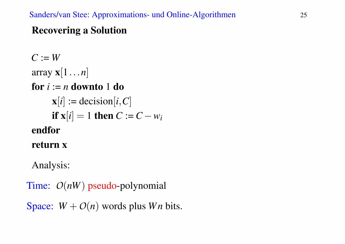
Recovering a Solution
C := Warray x[1 . . .n]for i := n downto 1 do
x[i] := decision[i,C]if x[i] = 1 then C := C−wi
endforreturn x
Analysis:
Time: O(nW ) pseudo-polynomial
Space: W +O(n) words plus Wn bits.
Sanders/van Stee: Approximations- und Online-Algorithmen 26
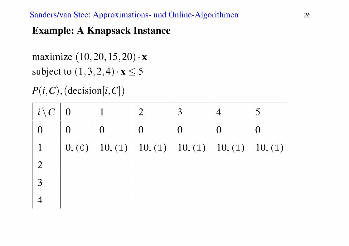
Example: A Knapsack Instance
maximize (10,20,15,20) ·xsubject to (1,3,2,4) ·x≤ 5
P(i,C),(decision[i,C])
i\C 0 1 2 3 4 5
0 0 0 0 0 0 0
1 0, (0) 10, (1) 10, (1) 10, (1) 10, (1) 10, (1)
2
3
4

Sanders/van Stee: Approximations- und Online-Algorithmen 27
Example: A Knapsack Instance
maximize (10,20,15,20) ·xsubject to (1,3,2,4) ·x≤ 5
P(i,C),(decision[i,C])
i\C 0 1 2 3 4 5
0 0 0 0 0 0 0
1 0, (0) 10, (1) 10, (1) 10, (1) 10, (1) 10, (1)
2 0, (0) 10, (0) 10, (0) 20, (1) 30, (1) 30, (1)
3
4

Sanders/van Stee: Approximations- und Online-Algorithmen 28
Example: A Knapsack Instance
maximize (10,20,15,20) ·xsubject to (1,3,2,4) ·x≤ 5
P(i,C),(decision[i,C])
i\C 0 1 2 3 4 5
0 0 0 0 0 0 0
1 0, (0) 10, (1) 10, (1) 10, (1) 10, (1) 10, (1)
2 0, (0) 10, (0) 10, (0) 20, (1) 30, (1) 30, (1)
3 0, (0) 10, (0) 15, (1) 25, (1) 30, (0) 35, (1)
4
Sanders/van Stee: Approximations- und Online-Algorithmen 29
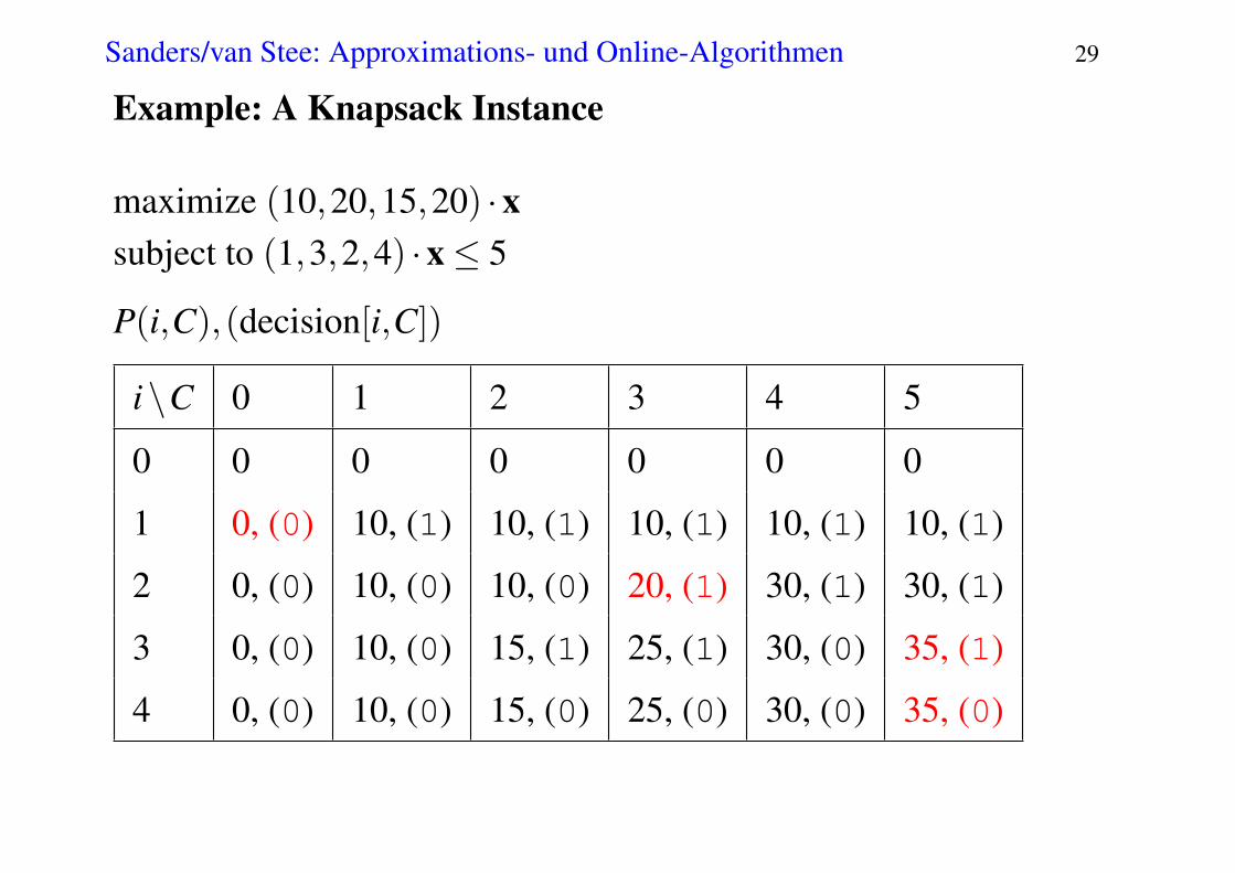
Example: A Knapsack Instance
maximize (10,20,15,20) ·xsubject to (1,3,2,4) ·x≤ 5
P(i,C),(decision[i,C])
i\C 0 1 2 3 4 5
0 0 0 0 0 0 0
1 0, (0) 10, (1) 10, (1) 10, (1) 10, (1) 10, (1)
2 0, (0) 10, (0) 10, (0) 20, (1) 30, (1) 30, (1)
3 0, (0) 10, (0) 15, (1) 25, (1) 30, (0) 35, (1)
4 0, (0) 10, (0) 15, (0) 25, (0) 30, (0) 35, (0)
Sanders/van Stee: Approximations- und Online-Algorithmen 30
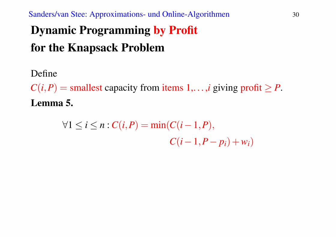
Dynamic Programming by Profitfor the Knapsack Problem
DefineC(i,P) = smallest capacity from items 1,. . . ,i giving profit ≥ P.
Lemma 5.
∀1≤ i≤ n : C(i,P) = min(C(i−1,P),
C(i−1,P− pi)+wi)

Sanders/van Stee: Approximations- und Online-Algorithmen 31
Dynamic Programming by Profit
Let P̂:= bp ·x∗c where x∗ is the optimal solution of the linearrelaxation.
Thus P̂ is the value (profit) of this solution.
Time: O(nP̂
)pseudo-polynomial
Space: P̂+O(n) words plus P̂n bits.

Sanders/van Stee: Approximations- und Online-Algorithmen 32
A Faster Algorithm
Dynamic programs are only pseudo-polynomial-time
A polynomial-time solution is not possible (unless P=NP...),because this problem is NP-hard
However, it would be possible if the numbers in the input weresmall (i.e. polynomial in n)
To get a good approximation in polynomial time, we are goingto ignore the least significant bits in the input
Sanders/van Stee: Approximations- und Online-Algorithmen 33
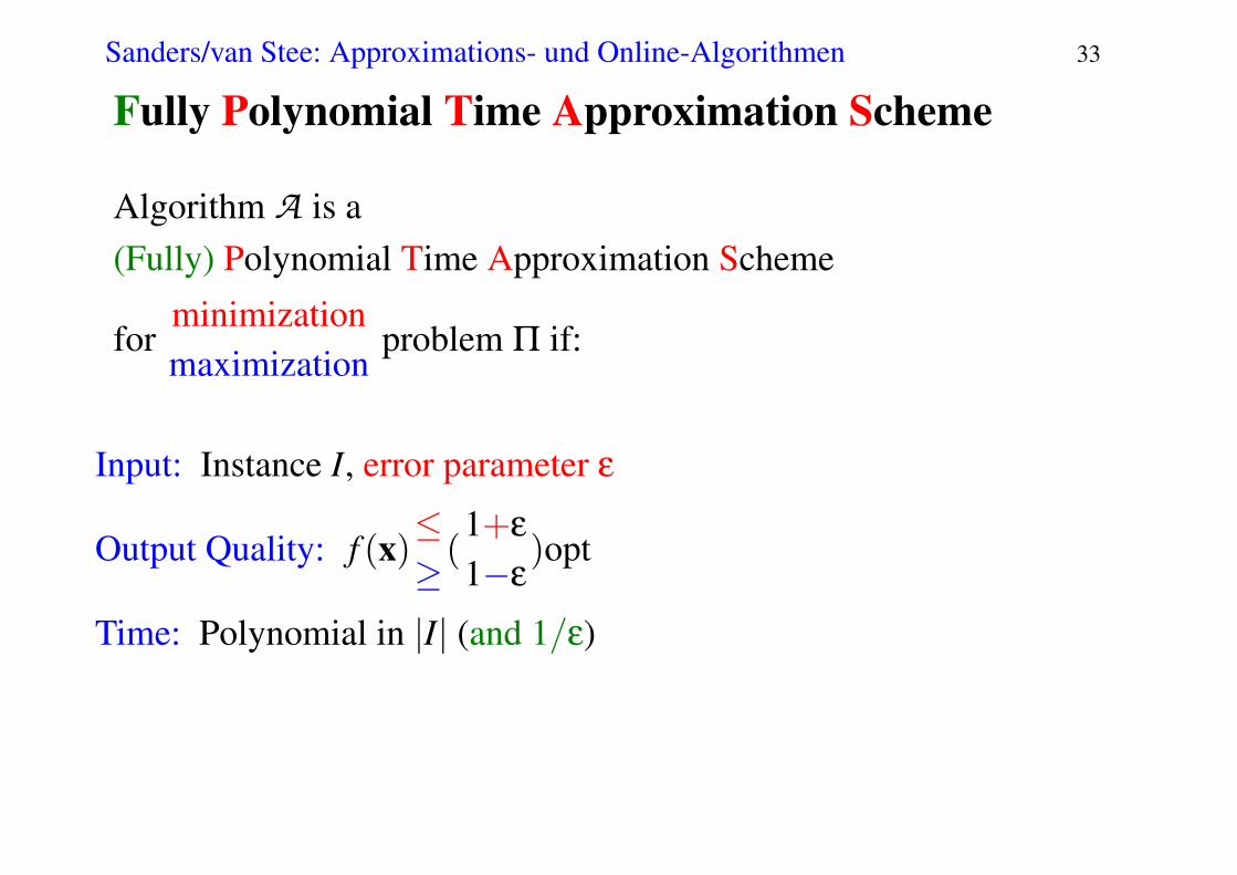
Fully Polynomial Time Approximation Scheme
Algorithm A is a(Fully) Polynomial Time Approximation Scheme
forminimizationmaximization
problem Π if:
Input: Instance I, error parameter ε
Output Quality: f (x)≤≥(
1+ε1−ε
)opt
Time: Polynomial in |I| (and 1/ε)
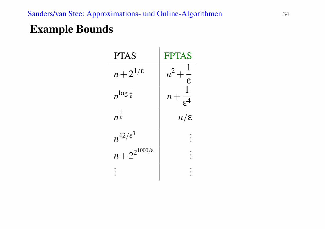
Sanders/van Stee: Approximations- und Online-Algorithmen 34
Example Bounds
PTAS FPTAS
n+21/ε n2 +1ε
nlog 1ε n+
1ε4
n1ε n/ε
n42/ε3 ...
n+221000/ε ......
...

Sanders/van Stee: Approximations- und Online-Algorithmen 35
FPTAS for Knapsack
P:= maxi pi // maximum profit
K:=εPn
// scaling factor
p′i:=⌊ pi
K
⌋// scale profits
x′:= dynamicProgrammingByProfit(p′,c,C)output x′

Sanders/van Stee: Approximations- und Online-Algorithmen 36
FPTAS for Knapsack
P:= maxi pi // maximum profit
K:=εPn
// scaling factor
p′i:=⌊ pi
K
⌋// scale profits
x′:= dynamicProgrammingByProfit(p′,c,C)output x′
Example:
ε = 1/3,n = 4,P = 20→ K = 5/3
p = (11,20,16,21)→ p′ = (6,12,9,12)
(equivalent to p′ = (2,4,3,4))
W
1121
1620

Sanders/van Stee: Approximations- und Online-Algorithmen 37
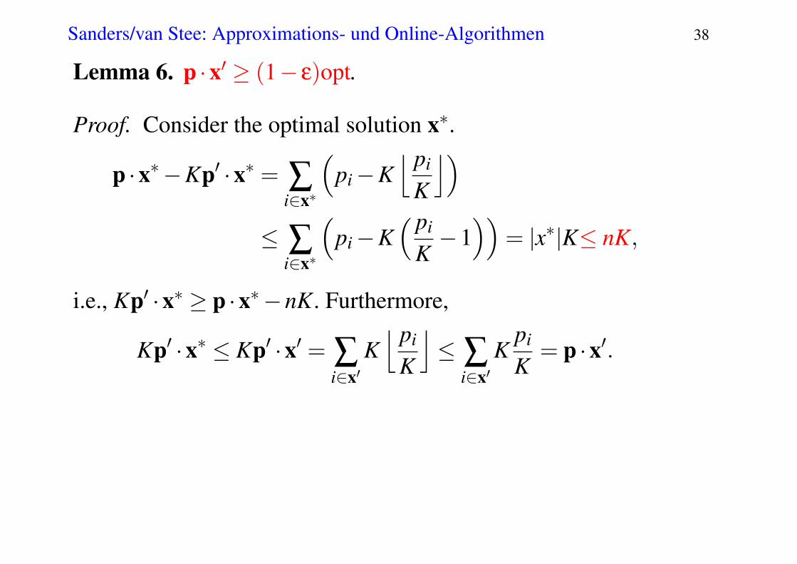
Lemma 6. p ·x′ ≥ (1− ε)opt.
Proof. Consider the optimal solution x∗.
p ·x∗−Kp′ ·x∗ = ∑i∈x∗
(pi−K
⌊ pi
K
⌋)
≤ ∑i∈x∗
(pi−K
( pi
K−1
))= |x∗|K≤ nK,
i.e., Kp′ ·x∗ ≥ p ·x∗−nK. Furthermore,
Kp′ ·x∗ ≤ Kp′ ·x′ = ∑i∈x′
K⌊ pi
K
⌋≤ ∑
i∈x′K
pi
K= p ·x′.
Hence,
p ·x′ ≥Kp′ ·x∗ ≥ p ·x∗−nK = opt− εP≥ (1− ε)opt
Sanders/van Stee: Approximations- und Online-Algorithmen 38
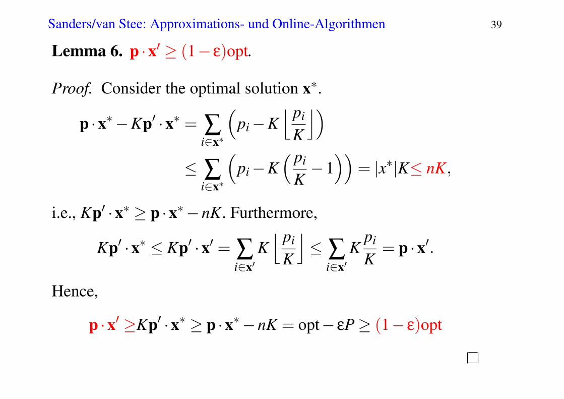
Lemma 6. p ·x′ ≥ (1− ε)opt.
Proof. Consider the optimal solution x∗.
p ·x∗−Kp′ ·x∗ = ∑i∈x∗
(pi−K
⌊ pi
K
⌋)
≤ ∑i∈x∗
(pi−K
( pi
K−1
))= |x∗|K≤ nK,
i.e., Kp′ ·x∗ ≥ p ·x∗−nK. Furthermore,
Kp′ ·x∗ ≤ Kp′ ·x′ = ∑i∈x′
K⌊ pi
K
⌋≤ ∑
i∈x′K
pi
K= p ·x′.
Hence,
p ·x′ ≥Kp′ ·x∗ ≥ p ·x∗−nK = opt− εP≥ (1− ε)opt
Sanders/van Stee: Approximations- und Online-Algorithmen 39
Lemma 6. p ·x′ ≥ (1− ε)opt.
Proof. Consider the optimal solution x∗.
p ·x∗−Kp′ ·x∗ = ∑i∈x∗
(pi−K
⌊ pi
K
⌋)
≤ ∑i∈x∗
(pi−K
( pi
K−1
))= |x∗|K≤ nK,
i.e., Kp′ ·x∗ ≥ p ·x∗−nK. Furthermore,
Kp′ ·x∗ ≤ Kp′ ·x′ = ∑i∈x′
K⌊ pi
K
⌋≤ ∑
i∈x′K
pi
K= p ·x′.
Hence,
p ·x′ ≥Kp′ ·x∗ ≥ p ·x∗−nK = opt− εP≥ (1− ε)opt

Sanders/van Stee: Approximations- und Online-Algorithmen 40
Lemma 7. Running time O(n3/ε
).
Proof. The running time of dynamic programming dominates.
Recall that this is O(
nP̂′)
where P̂′ = bp′ ·x∗c.We have
nP̂′ ≤n · (n ·max p′i) = n2⌊
PK
⌋= n2
⌊PnεP
⌋≤ n3
ε.
Sanders/van Stee: Approximations- und Online-Algorithmen 41
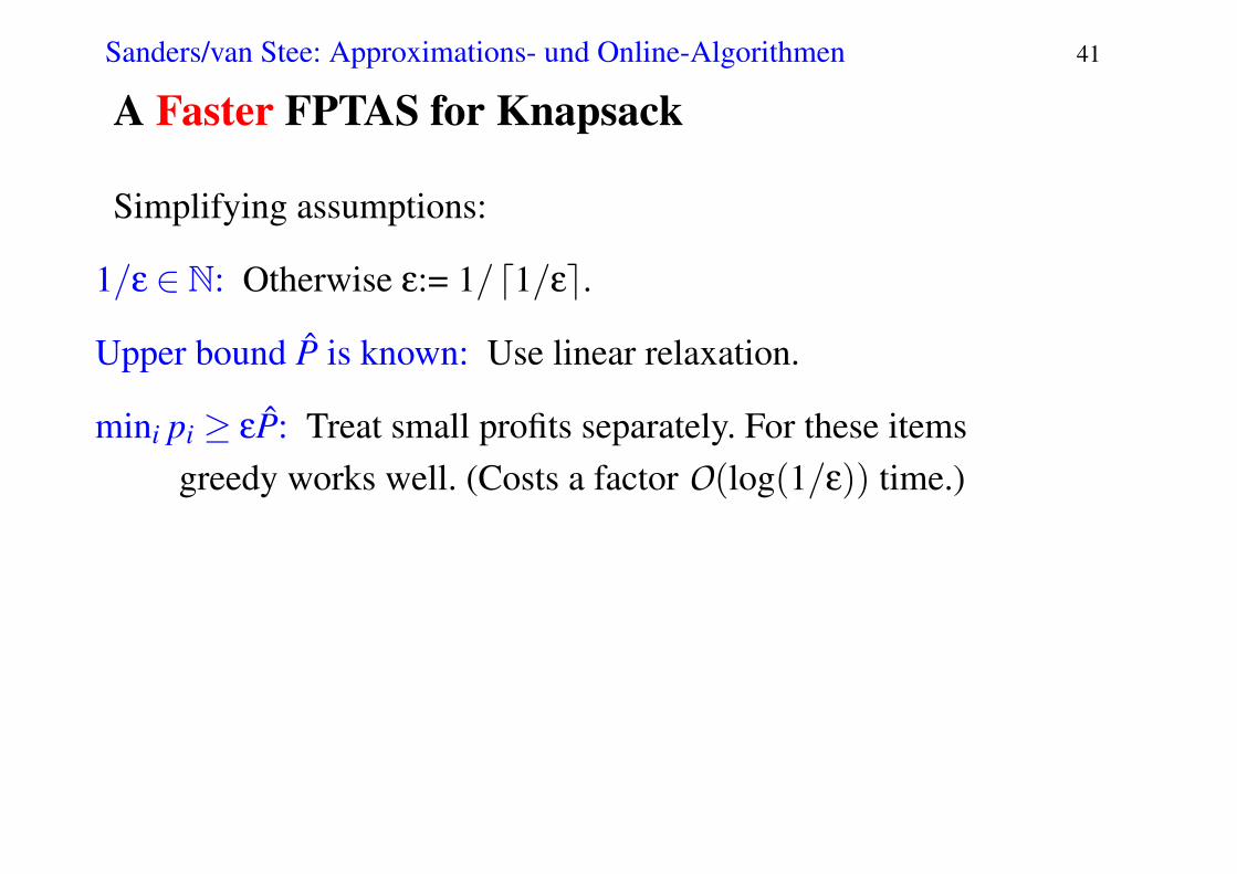
A Faster FPTAS for Knapsack
Simplifying assumptions:
1/ε ∈ N: Otherwise ε:= 1/d1/εe.Upper bound P̂ is known: Use linear relaxation.
mini pi ≥ εP̂: Treat small profits separately. For these itemsgreedy works well. (Costs a factor O(log(1/ε)) time.)

Sanders/van Stee: Approximations- und Online-Algorithmen 42
A Faster FPTAS for Knapsack
M:=1ε2 ; K:= P̂ε2 = P̂/M
p′i:=⌊ pi
K
⌋// p′i ∈
{1ε , . . . ,M
}
value of optimal solution was P̂, is now MC j:= {i ∈ 1..n : p′i = j}remove all but the
⌊Mj
⌋lightest (smallest) items from C j
do dynamic programming on the remaining items
Lemma 8. px′ ≥ (1− ε)opt.
Proof. Similar as before, note that |x| ≤ 1/ε for anysolution.

Sanders/van Stee: Approximations- und Online-Algorithmen 43
Lemma 9. Running time O(n+Poly(1/ε)).
Proof.
preprocessing time: O(n)
values: M = 1/ε2
pieces:M
∑i=1/ε
⌊Mj
⌋≤M
M
∑i=1/ε
1j≤M lnM = O
(log(1/ε)
ε2
)
time dynamic programming: O(
log(1/ε)ε4
)

Sanders/van Stee: Approximations- und Online-Algorithmen 44
The Best Known FPTAS
[Kellerer, Pferschy 04]
O
(min
{n log
1ε
+log2 1
εε3 , . . .
})
• Less buckets C j (nonuniform)
• Sophisticated dynamic programming
Sanders/van Stee: Approximations- und Online-Algorithmen 45
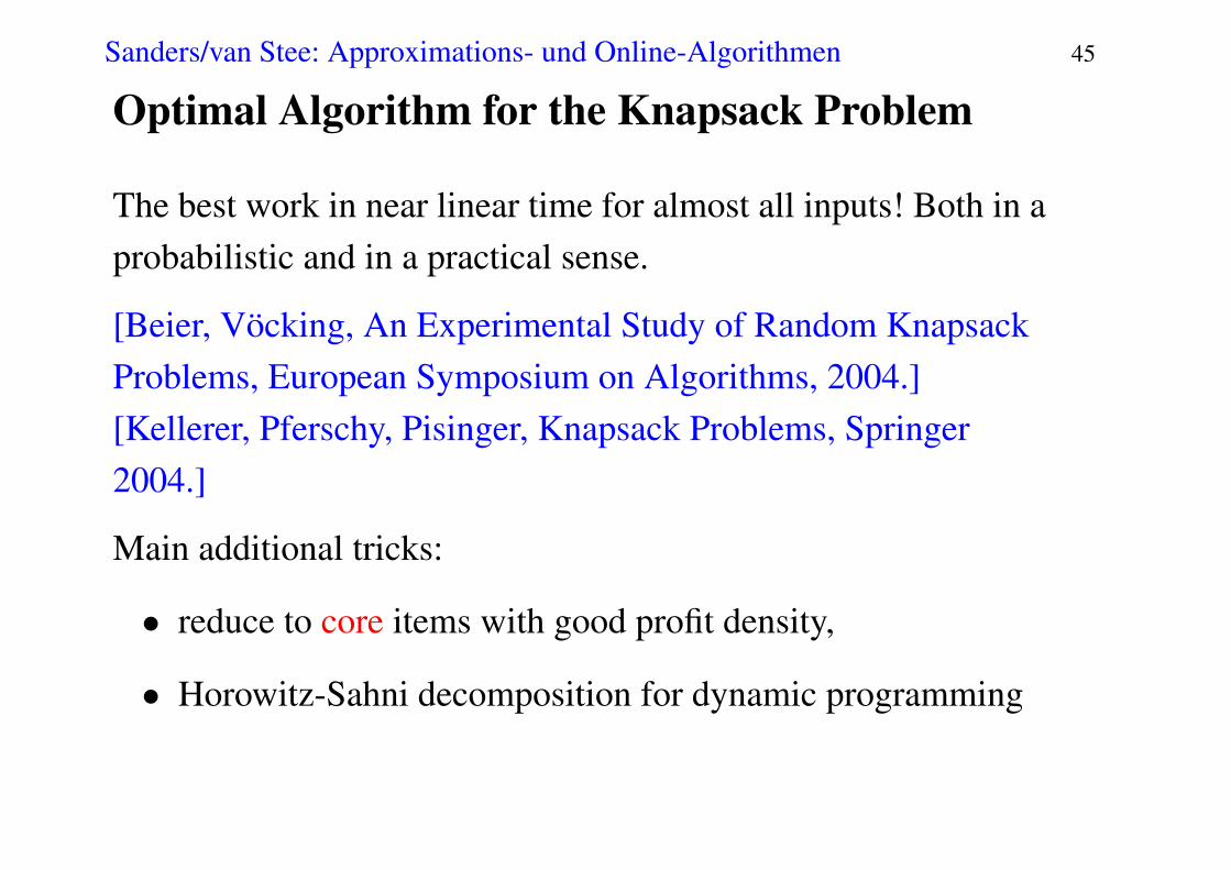
Optimal Algorithm for the Knapsack Problem
The best work in near linear time for almost all inputs! Both in aprobabilistic and in a practical sense.
[Beier, Vöcking, An Experimental Study of Random KnapsackProblems, European Symposium on Algorithms, 2004.][Kellerer, Pferschy, Pisinger, Knapsack Problems, Springer2004.]
Main additional tricks:
• reduce to core items with good profit density,
• Horowitz-Sahni decomposition for dynamic programming
Sanders/van Stee: Approximations- und Online-Algorithmen 46
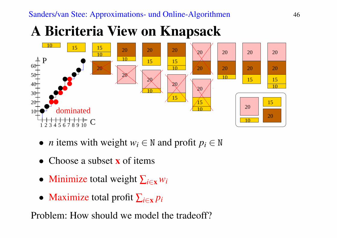
A Bicriteria View on Knapsack
dominated
10 15 1510
20
10
20
15
20
1510
20
20
10
20
20
15
20
20
1510
2020
1020
15
20
2020
20
1510 20
10
15
2010
20
30
40
50
60
1 2 3 4 5 6 7 8 9 10 C
P
• n items with weight wi ∈ N and profit pi ∈ N
• Choose a subset x of items
• Minimize total weight ∑i∈x wi
• Maximize total profit ∑i∈x pi
Problem: How should we model the tradeoff?

Sanders/van Stee: Approximations- und Online-Algorithmen 47
Pareto Optimal Solutions[Vilfredo Frederico Pareto (gebürtig Wilfried Fritz)* 15. Juli 1848 in Paris, † 19. August 1923 in Céligny]Solution x dominates solution x′ iff
p ·x≥ p ·x′∧ c ·x≤ c ·x′
and one of the inequalities is proper.
Solution x is Pareto optimal if
6 ∃x′ : x′ dominates x
Natural Question: Find all Pareto optimal solutions.

Sanders/van Stee: Approximations- und Online-Algorithmen 48
In General
• d objectives
• various problems
• various objective functions
• arbitrary mix of minimization and maximization

Sanders/van Stee: Approximations- und Online-Algorithmen 49
Enumerating only Pareto Optimal Solutions
[Nemhauser Ullmann 69]
L := 〈(0,0)〉 // invariant: L is sorted by weight and profitfor i := 1 to n do
L ′:= 〈(w+wi, p+ pi) : (w, p) ∈ L〉 // time O(|L |)L := merge(L ,L ′) // time O(|L |)scan L and eliminate dominated solutions // time O(|L |)
• Now we easily lookup optimal solutions for variousconstraints on C or P
• We can prune L if a constraint is known beforehand
Sanders/van Stee: Approximations- und Online-Algorithmen 50
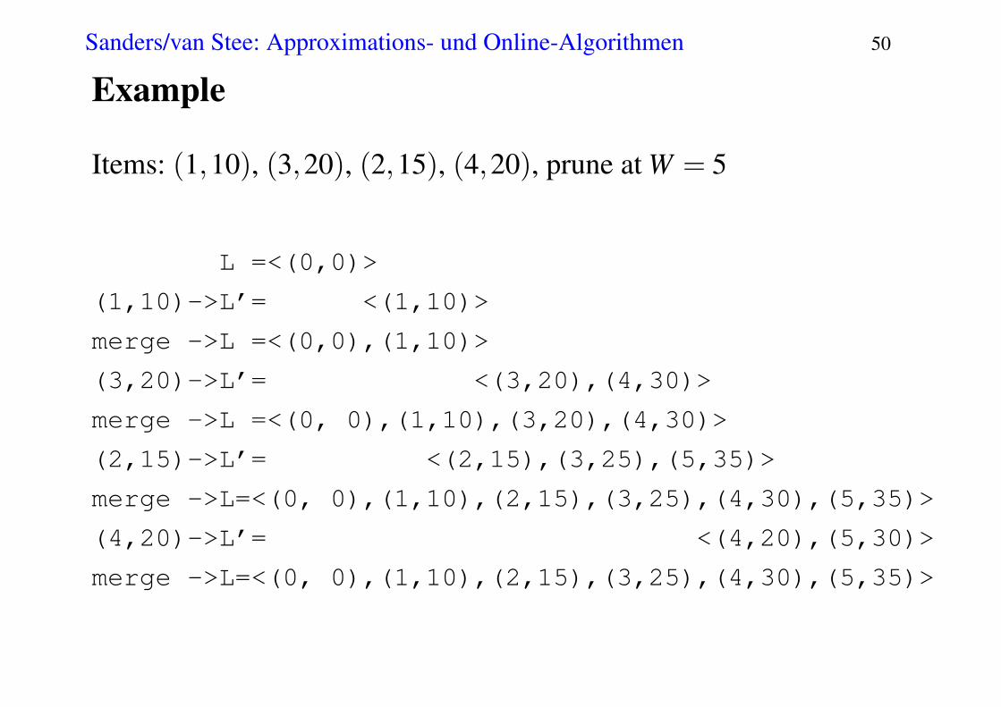
Example
Items: (1,10), (3,20), (2,15), (4,20), prune at W = 5
L =<(0,0)>
(1,10)->L’= <(1,10)>
merge ->L =<(0,0),(1,10)>
(3,20)->L’= <(3,20),(4,30)>
merge ->L =<(0, 0),(1,10),(3,20),(4,30)>
(2,15)->L’= <(2,15),(3,25),(5,35)>
merge ->L=<(0, 0),(1,10),(2,15),(3,25),(4,30),(5,35)>
(4,20)->L’= <(4,20),(5,30)>
merge ->L=<(0, 0),(1,10),(2,15),(3,25),(4,30),(5,35)>
Sanders/van Stee: Approximations- und Online-Algorithmen 51
Horowitz-Sahni Decomposition
• Partition items into two sets A, B
• Find all Pareto optimal solutions for A, LA
• Find all Pareto optimal solution for B, LB
• The overall optimum is a combination of solutions from LA
and LB. Can be found in time O(|LA|+ |LB|)• |LA| ≤ 2n/2
Question: What is the problem in generalizing to three (ormore) subsets?