Oceanside Littoral C

ell

ESCONDIDO CREEK

SAN DIEGO RIVER

OTAY RIVER

LOS PENASQUITOS CREEK

TIJUANA RIVER

LUSARDI CREEK

RIO TIJUANA

-75

-25

-50

-500

-475

-525

-450

-550

-425

-400

-575

-375

-350

-325

-300

-275

-250

-225

-600

-200

-175

-150

-100

-125

-625

-650

-675

-700

-725

-750

-775

-800

-825

-850-875 -900

-925

-950-975

-102

5

-1050-1075

-1100

-1150-1175

-1200

-1225

0

-350

-1225

-150

-400

-150

-250

-225

-900

-175

-350

-950

-125

0

-100-125

-150

-925

0 10 205 Kilometers

Mexico

La Jolla

San Diego

Pt. LomaPLOO

SBOO

Islas Coronados

9 Mile Bank

Silver Strand Cell

Mission Bay Subcell

La JollaCanyon

Loma Sea Valley

Coronado Canyon

Tijuana River

Mission Bay

SDBay

Figure 1. Map of marine shelf of San Diego County. Bathymetric units are meters. Locations of littoral cells, submarine canyons, outfalls (PLOO and SBOO), rivers, and Kelp Forests (shaded areas close to shore) are indicated.

0 6 123 Kilometers

LA-5

-50

-75

-25

-100

-125

-150

-175

-200

-225

-250

-275

-300

-325

-350-375-400

E9

E3

E7

E1

B8

E8

E5

E2

B9

B13

E21

E15

B10

E19

B11

E26

E25

E23

E17

E11

B12

E20

E14

Figure 2. Map of benthic monitoring stations offshore of Pt. Loma. Bathymetric units are meters. The location of the LA-5 dredge disposal site is also indicated.

0 6 123 Kilometers

LA-5

-50

-75

-25

-100

-125

-150

-175

-200

-225

-250

-275

-300

-325

-350

-375-400

-275

SD9 SD6

SD3

SD1

SD8

SD14

SD13

SD12

SD10

SD11

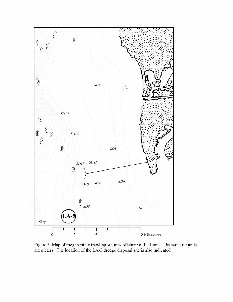
Figure 3. Map of megabenthic trawling stations offshore of Pt. Loma. Bathymetric units are meters. The location of the LA-5 dredge disposal site is also indicated.

0 6 123 Kilometers

LA-5

-50

-75

-25

-100

-125

-150

-175

-200

-225

-250

-275

-300

-325

-350

-375-400

-275

SD9

SD8

RF2

RF1

SD14

SD13

SD12

SD10

SD11

Figure 4. Map of bioaccumulation study sites offshore of Pt. Loma. Bathymetric units are meters. The location of the LA-5 dredge disposal site is also indicated.

(

(

(

(

(

(

(

(

(

(

(

(

(

(

(

(

(

(

(

(

(

(

(

(

(

LA-4

LA-5SEDsAll EventsPHImedian

1.700000 - 2.200000

2.200001 - 2.700000

2.700001 - 3.200000

3.200001 - 3.700000

3.700001 - 4.200000

Figure 5. Mean of median grain sizes (PHI) for PLOO sediment stations. Note, PHI increases with decreasing grain size.

Figure 6. Satellite imagery of Pt. Loma during the period that the outfall was ruptured in 1992. Note the spatial distribution of waters emanating from Mission and San Diego Bays, and the current reversal of plume. False color represents surface temperatures. Warmer temperatures are indicated by red.

(

(

!

!

!

!

!

!

!

!

!

!

!

!

!

!

!

!

!

!

!

!

!

!

!

LA-4

LA-5

sdbackscatterValue

High : 248.447449

Low : 99.524330

Figure 7. Spatial distribution of backscatter on the shelf off San Diego. Data are from a studyby Gardner et al. (1998).

B11

B8

E19

E7

E1

B12B9E26

E25E23

E20

E14

E17E11

E8E5

E2

B13

B10E21

E15

E9

E3

Stress: 0.02

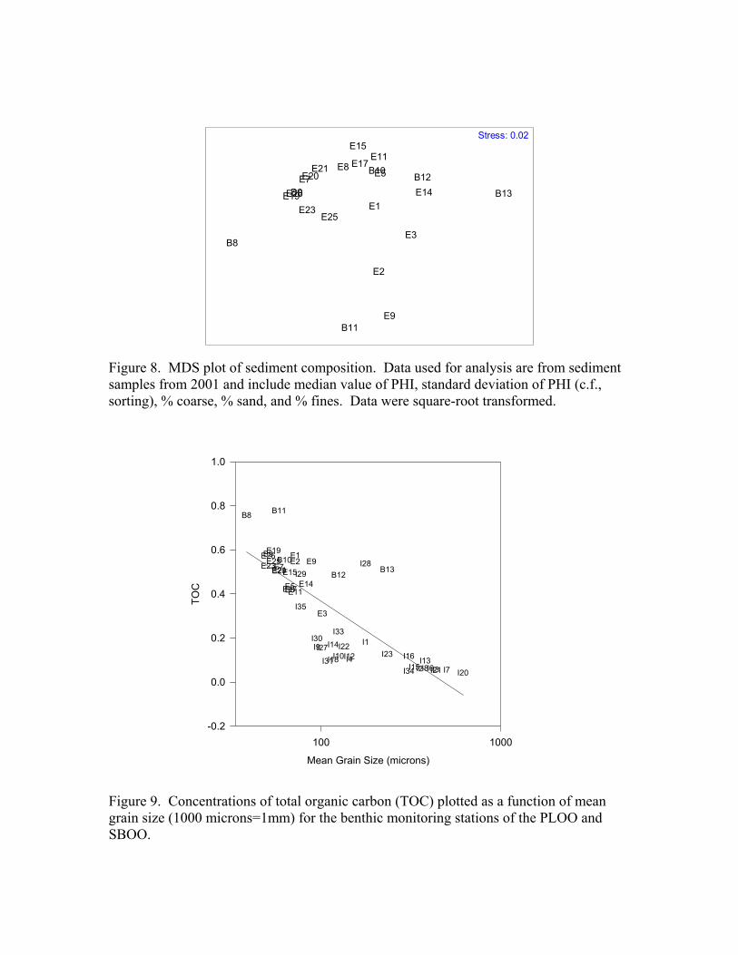
Figure 8. MDS plot of sediment composition. Data used for analysis are from sediment samples from 2001 and include median value of PHI, standard deviation of PHI (c.f., sorting), % coarse, % sand, and % fines. Data were square-root transformed.

Mean Grain Size (microns)

100 1000

TOC

-0.2

0.0

0.2

0.4

0.6

0.8

1.0

I35

I34I31

I23I18I10 I4

I33I30

I27 I22I14

I15I16I12

I9

I6I3

I29

I21I13I8I2

I28

I20I7

I1

B9

B12

E2

E5E8E11E14E17

E20E23E25E26

B8 B11

E1E7

E19B10

E3

E9E15E21 B13

Figure 9. Concentrations of total organic carbon (TOC) plotted as a function of mean grain size (1000 microns=1mm) for the benthic monitoring stations of the PLOO and SBOO.

(

(

(

(

(

(

(

(

(

(

(

(

(

(

(

(

(

(

(

(

(

(

(

(

(

_ __

_

_

_ __

_

__

___ _

_ __ _

_

_ _ _ _

__

_

LA-4

LA-5

0 9 184.5 Kilometers

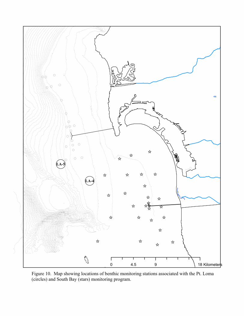
Figure 10. Map showing locations of benthic monitoring stations associated with the Pt. Loma (circles) and South Bay (stars) monitoring program.

B11

B8

E19E7

E1

B12B9

E26E25E23 E20

E14

E17E11

E8

E5

E2

B13

B10

E21E15E9

E3

Stress: 0.01

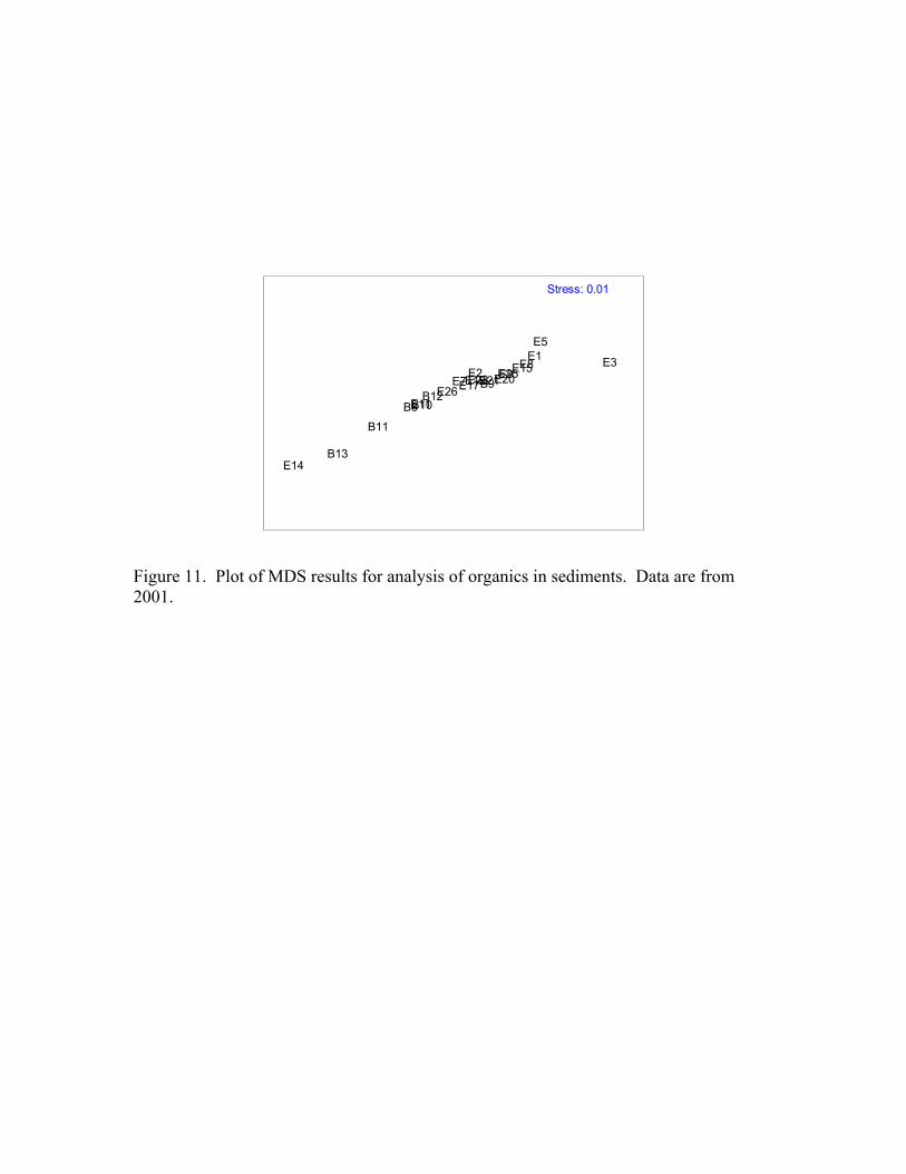
Figure 11. Plot of MDS results for analysis of organics in sediments. Data are from 2001.

Figure 12. Map indicating sediment transport in the Silver Strand Littoral Cell (from Inman, 1976). Zones of sediment accretion and erosion are indicated. Bathymetric units are feet.

(

(LA-4

LA-5

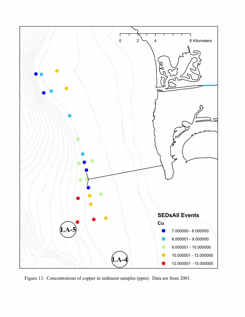
0 4 82 Kilometers

SEDsAll EventsCu

7.000000 - 8.000000

8.000001 - 9.000000

9.000001 - 10.000000

10.000001 - 12.000000

12.000001 - 15.000000

Figure 13. Concentrations of copper in sediment samples (ppm). Data are from 2001.

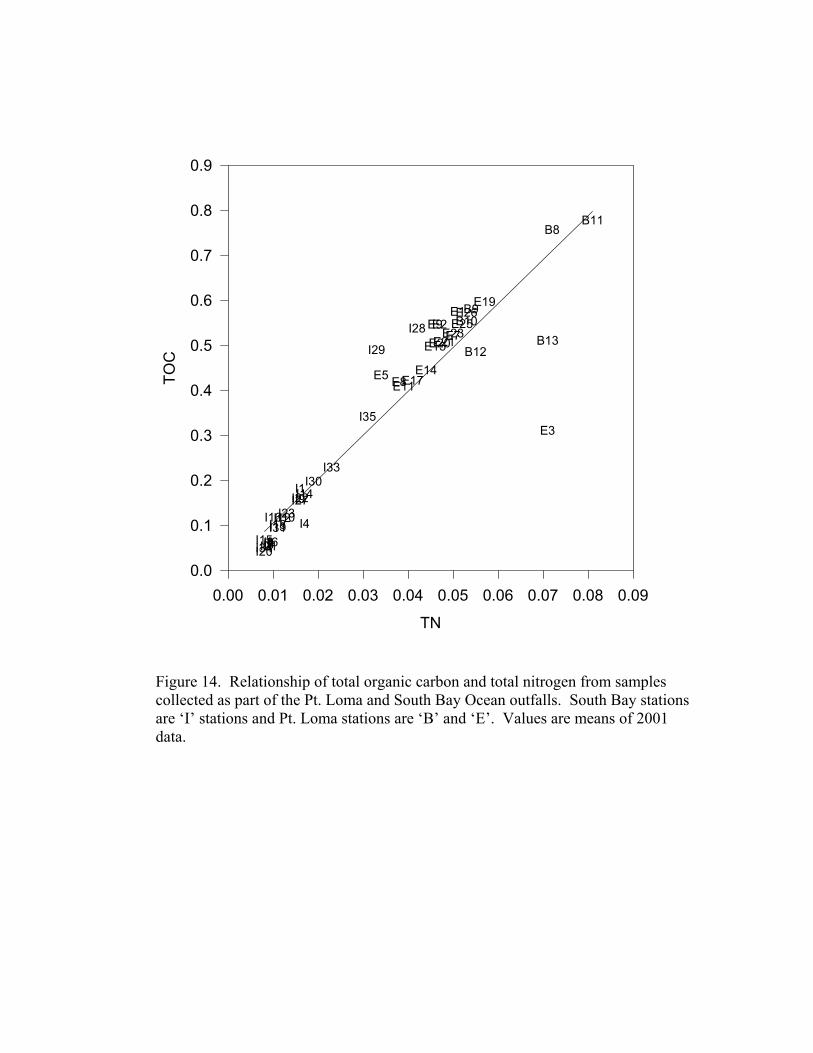
TN

0.00 0.01 0.02 0.03 0.04 0.05 0.06 0.07 0.08 0.09

TOC

0.0

0.1

0.2

0.3

0.4

0.5

0.6

0.7

0.8

0.9

I35

I34I31

I23I18I10 I4

I33I30

I27I22I14

I15

I16I12I9

I6I3

I29

I21I13

I8I2

I28

I20I7

I1

B9

B12

E2

E5 E8E11E14

E17

E20E23

E25E26

B8B11

E1

E7

E19B10

E3

E9

E15E21 B13

Figure 14. Relationship of total organic carbon and total nitrogen from samples collected as part of the Pt. Loma and South Bay Ocean outfalls. South Bay stations are ‘I’ stations and Pt. Loma stations are ‘B’ and ‘E’. Values are means of 2001 data.

Figure 15. Backscatter image showing spatial distribution of dredge disposal mounds (outlined in red). Dark circle with concentric lighter circle is the LA-5 dredge disposal site. The Pt. Loma Ocean Outfall is clearly visible. Survey from Gardner et al., 1998).

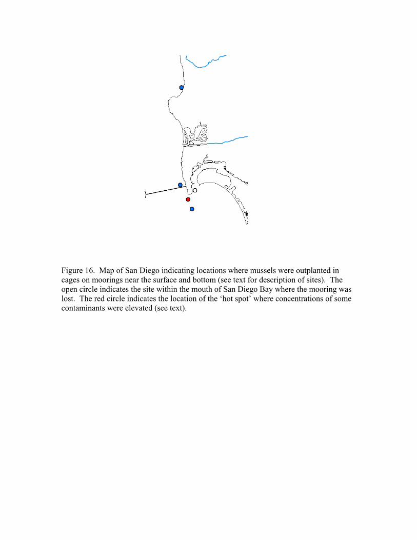
Figure 16. Map of San Diego indicating locations where mussels were outplanted in cages on moorings near the surface and bottom (see text for description of sites). The open circle indicates the site within the mouth of San Diego Bay where the mooring was lost. The red circle indicates the location of the ‘hot spot’ where concentrations of some contaminants were elevated (see text).

Figure 17. Results of MDS analysis. Analytes used in the analysis included organics, heavy metals, and PCB’s in mussel tissue. A site near the Scripps pier was used as a reference site. All samples at all depths, except for the reference spot and the bottom sample near the mouth of the San Diego Bay (indicated by red circle in Fig. 15 and by “PL2_8m” in this figure), clustered closely together. A stress level of zero indicates that the results are unambiguous.

Scripps

PL1_3mPL1_8mPL2_3m

PL2_8m

PL3_8mPL3_12m

Stress: <0.001