sampling power-law distributions - eprintseprints.soton.ac.uk/40880/1/pickeringetal.pdf ·...

E L S E V I E R Tectonophysics 248 (1995) 1-20

TECTONOPHYSICS

Sampling power-law distributions

G. Pickering *, J.M. Bull, D.J. Sanderson Department of Geology, University of Southampton, Highfield, Southampton, S017 1B J, UK

Received 30 August 1994; accepted 10 March 1995

Abstract

Power-law distributions describe many phenomena related to rock fracture. Data collected to measure the parameters of such distributions only represent samples from some underlying population. Without proper consideration of the scale and size limitations of such data, estimates of the population parameters, particularly the exponent D, are likely to be biased. A Monte Carlo simulation of the sampling and analysis process has been made, to test the accuracy of the most common methods of analysis and to quantify the confidence interval for D. The cumulative graph is almost always biased by the scale limitations of the data and can appear non-linear, even when the sample is ideally power law. An iterative correction procedure is outlined which is generally successful in giving unbiased estimates of D. A standard discrete frequency graph has been found to be highly inaccurate, and its use is not recommended. The methods normally used for earthquake magnitudes, such as a discrete frequency graph of logs of values and various maximum likelihood formulations can be used for other types of data, and with care accurate results are possible. Empirical equations are given for the confidence limits on estimates of D, as a function of sample size, the scale range of the data and the method of analysis used. The predictions of the simulations are found to match the results from real sample D-value distributions. The application of the analysis techniques is illustrated with data examples from earthquake and fault population studies.

1. Introduct ion

Many objects that occur naturally over different scales show a power-law distribution of rela- tive abundance (Schroeder, 1991). This is particularly true for phenomena related to rock fracture such as earthquakes (Gutenberg and Richter, 1954), fault displacements (Kakimi, 1980), fault and fracture trace lengths (Heifer and Bevan,

* Corresponding author

1990) and fracture apertures (Barton and Zoback, 1992). In all of these papers the data represent samples from some underlying distribution. It is the parameters describing this distribution that are required to help our theoretical understand- ing of the processes involved and enable predictions from such theory. Therefore, it is crucial to know whether the analysis of samples can give us unbiased estimates of the distribution parameters, and how precise these unbiased estimates are. This paper gives a detailed description of the common sample biases and how these affect the analysis of samples from power-law distributions. Using Monte Carlo simulation of the sampling

0040-1951/95/$09.50 © 1995 Elsevier Science B.V. All rights reserved SSDI 0040-1951(95)00030-5

2 G. Pickering et aL / Tectonophysics 248 (1995) 1-20

process, the parameters derived from samples can be tested for bias and the random error quantified. With real data there is also the problem of testing whether the power-law distribution is an appropriate model. This question is ad- dressed and the results of the simulation are illustrated using examples from earthquake and fault population studies.

2. Power-law distributions

There are three commonly used definitions of a power-law distribution. In many fault population studies the cumulative distribution Junction is used e.g., Childs et al. (1990), Walsh et al. (1991) and Jackson and Sanderson (1992):

N = a l u-b, (1)

where u is a measure of size and N is the cumulative number of values > u, a~ is a constant and b I is the exponent (Fig. la). An alternative is to define the model in terms of the discrete frequency distribution, e.g., Kakimi (1980), Heifer and Bevan (1990) and Barton and Zoback (1992):

n = a2 u - b 2 (2)

where n is the frequency of values in an interval u + 3u (Fig. lb). A third definition is to use the discrete frequency of log u:

log ntg = a 3 - b31og u (3)

where nlg is the frequency of values in an interval log u _+ 8(log u) (Fig. lc). This is most common in earthquake studies, and is probably bet ter known as the Gutenberg-Rich te r relationship (Guten- berg and Richter, 1954), where earthquake magnitude, M is substituted for log u. Note that this is not equivalent to the logarithmic of (2) as the definition of n in the two equations is different.

Any at tempt to fit data to the model given by (2) must use a finite interval size 8u. Definition (2) is an idealised form where 6u --* 0. The function for n can be derived from N assuming a

finite interval 8u and using the binomial expan- sion, neglecting all second-order terms and above:

n = ~ N = N > _ , - N ~ , , + a , , ~ = u b _ ( u +Su) -~

(4)

by assuming 8u << u, then:

n = a l b l u (t"+l)SU (5)

Consequently, any real n will depend on the interval size flu. If logs are taken of (5) the interval size becomes an additional constant, and the gradient will give - ( b 1 + 1 )= - b 2. There is an additional problem with using (2), in that it assumes that small changes in u (i.e. u + 8u) cause a change in n. This is reasonable at the small scale where the distribution is virtually con- tinuous, but will break down at the large scale as the distribution is sparse. At the large scales, the model predicts fractional values for n, whereas real values of n will be 0 or 1. This can be seen on discrete frequency graphs as will be shown later. The cumulative distribution N is independent of interval size and can describe the distribution at all scales.

Some authors (e.g., Bender, 1983) have claimed that the cumulative function cannot describe real data, as it assumes an infinite maximum value to the distribution. However, if N is restricted to integer values of 1 or more, then the maximum value will be determined by N = 1, and the distribution is bounded at the large scale. Bath (1981) has suggested that (3) is the best description of the true earthquake magnitude distribution. The cumulative distribution derived in Baths paper from (3) is non-linear, however, a linear log-interval distribution can be derived from the integer cumulative definition (1). If we take two cumulative numbers, N 2 > Nj where:

N 2 = a l u 2 bl

N 1 = a l U l bl

then:

N 2 - N l = a l (u f bl - u[ b,)

("~t b' 1 =alu2bl[1-- \U2] ]

(6)

(7)

G. Pickering et aL / Tectonophysics 248 (1995) 1-20 3

(a)

(b)

al

N

a 2

taking logs:

l og (N 2 - N1) = log a I - bllog u 2

where N 2 - N 1 is the number in the interval u~ ~ u 2. If we take constant log intervals (Slog u then:

(u -~2)=lO~(~°g") ;N2-N,=nlg (9)

If the two constant terms are combined and set equal to some value 7, then:

log nlg = Y - bllog u2 (10)

Therefore, the integer cumulative definition is consistent with a linear log-interval graph, where b 3 = b 1. The non-linearity seen in cumulative graphs, which has lead several authors to suggest alternative functions for such graphs [see Bath (1981) for a review], is due to sampling effects and will be discussed later. Given the basic com- patibility of all three distributions, the integer cumulative definition is our preferred model, as it can describe the distribution at all scales, is independent of interval choice and embodies the hierarchial nature of power-law distributions. This is used to produce all the simulated data. To main- tain a consistency of notation with Jackson and Sanderson (1992) and Pickering et al. (1994), this distribution is described with an exponent D and a constant c.

(c)

a3

%

U

3. Sampling effects

All data sets represent samples from a population of values. If this sample excludes certain types of values the sample is biased, and is not representative of the population. Most samples are limited in areal extent (and time with respect

Fig. 1. Schematic graphs of the three commonly used definitions of a power-law distribution on log axes. (a) Cumulative frequency (Eq. 1). (b) Discrete frequency (Eq. 2). (c) Discrete frequency of log (u) or log interval (Eq. 3).

4 G. Pickering et al./Tectonophysics 248 (1995) 1-20

to earthquakes), size and scale range, and are therefore biased. There are two common biases in rock fracture studies, truncation and censoring (Einstein and Baecher, 1983). In the following discussion and the remainder of the paper, scale range refers to the difference in value between the maximum and minimum of the sample, and size or size range to the number of values within the sample.

3.1. Truncation

If the scale range of a sample is less than that of the population as a whole then the sample is truncated. Most samples from geological power- law distributions are truncated. At the small scale this is known as left-hand truncation (LHT) and is usually related to the resolution of the method of measurement; earthquake magnitudes, for example, are limited by the sensitivity of the seis- mographs used. Associated with this L H T is a loss of data as the limit of sensitivity is approached. This is called the L H T "fall-off". Data within this "fall-off" axe not representative of the distribution and should be excluded from the analysis. If this is done, corrections such as that given in Barton and Zoback (1992), are unneces- sary.

Large-scale or right-hand truncation (RHT) is also common, although it is less often recognised. A hanging-wall or footwall cutoff of a large fault may not be visible or may be lost due to erosion. Earthquake data recorded over a limited time will often miss rare large events. The problem of truncation is particularly common when sampling from power-law distributions, as they often ex- tend over a large scale range, where the majority of values in the distribution may be beyond that of the scale range of observation.

3.2. Censoring

A sample is censored when some, or all, of the values within it are systematically under-or over- estimated. The classic example of censored data is in life testing, where if some test units have not failed at the end of the experiment, their true

"'life" is unknown, only that it is greater than the length of time of the experiment (Nelson and Hahn, 1972, 1973). Most fracture length statistics are affected by censoring. Three types can be defined:

Type A: As no fracture can have a measured length larger than that of the survey, the length of fractures which are longer than the maximum dimension of the survey will be underestimated.

Type B: If one end of the fracture lies beyond the boundary of the survey the measured length will underest imate the true length. This problem is more likely to occur for longer fractures but may affect fractures of any size.

Type C: If there is a restriction on the minimum displacement or width that can be observed (left-hand truncation) then the fracture tips will not be observed. Therefore, every fracture length will be underestimated.

Methods have been developed to find the true distribution from censored data [see Laslett (1982) for review]. They have mainly been concerned with log-normal or negative exponential distributions, e.g., Cruden (1977), Priest and Hudson (1981) and Einstein and Baecher (1983). For a power-law distribution of lengths, types A and B are not usually a serious problem. This is because within any given scale range, there are always more small values than large values in a power-law distribution. Short fractures cannot suffer from Type A censoring, and are less likely to suffer from Type B, and these will make up the majority of the data available. In contrast, Type C censoring is most serious for small fractures. As the truncation cutoff is similar for all fractures, a larger proportion of the length of a small fracture will have displacement /width less than the cutoff. This problem makes reliable estimation of the true distribution impossible, unless the data are corrected.

Walsh and Watterson (1988) and Heifer and Bevan (1990) suggest similar solutions, by correcting each measurement for an estimated "missing" length. This is achieved by assuming relationships between (a) d isplacement /width and radial dis- tance from the centre of the fracture and (b) the maximum displacement /width and length; details are contained in Heffer and Bevan (1990).

G. Pickering et al. / Tectonophysics 248 (1995) 1-20 5

Other sampling problems are usually specific to the sampling methods or the particular properties under examination. Examples of these include earthquake magnitude saturation, e.g., Frochlich and Davis (1993), and multi-line sampling of fault displacements (Yielding et al., 1992; Pickering et al., in press). There may also be problems of distinguishing individual fractures from close spaced sets of fractures, e.g., Barton and Zoback (1992). This leads to an overestimate of the density of large-scale fractures, which can be corrected using the method given in the paper of Barton and Zoback. Although referred to as censoring, the effect is distinctly different from the original definition of under-or overestimating individual values, and their correction cannot be used for any of the types of censoring (A, B, C) defined earlier. Such problems should be resolved before analysing the data, by either excluding the affected data from the analysis (e.g., satu- rated magnitudes) or correcting for the bias introduced.

4. Methods of analysis

If biases introduced by censoring and other sample specific effects are minimal or have been corrected, samples from power-law populations will still suffer from truncation. In this section we discuss the use of various analysis methods in the light of this truncation and other sampling effects.

4.1. Cumulat ive frequency method

A log transform of (1) gives a simple linear relationship between log N and log u. Any LHT fall-off is easily detected as it will cause a deviation at the small scale; the rest of the data should fall on a straight line. However, there is often a systematic deviation at the large scale on many cumulative graphs (Fig. 2a). This can be at- tributed to the truncation of the sample. This deviation has been called "censoring" (Jackson and Sanderson, 1992; Pickering et al., 1994), but

that term should be reserved for the problems outlined earlier and a more appropriate term is the finite-range effect.

Three idealised non-random samples derived from an integer power-law distribution with D = 1.0 and a maximum value of 10,000 are shown in Fig. 3. Sample A, of size 100, has a maximum value of 100 and a minimum at 1; it plots on the cumulative graph giving an exact fit to a line with a slope of 1. Sample B has the same RHT at 100, but a minimum at 10 and shows a deviation. Even if a line was fitted to the semi-linear part at the small scale, the slope would overestimate the distribution D-value. The difference between the two samples is the amount that the scale range and size range have been reduced in comparison to the original distribution. For sample A they have been reduced equally by 1/100. For sample B the size has been reduced by 1/1001 but the scale range has been reduced by 1/1000. Sample A is "self-similar" to the distribution whereas sample B is not. In the alternative case, where the scale range is reduced by less than the reduction in size range, the graph may underestimate the D-value. However, this case is rare with real data as it is often much easier to increase the size of the data set, rather than its scale range.

The solution to this problem is based on the observation that self-similar samples produce undistorted graphs. Consider sample C (see Fig. 3), which is sample A with the ten largest values removed, but it could equally well have been derived from the original distribution. In the self-similar Sample A, these data were assigned values of N from 11 to 100. Therefore, if for sample C we began counting from 11, the distor- tion would be removed and the graph would give a slope of 1. This "correction" can be predicted using the following derivation for a general power law.

The line of a self-similar sample from a power- law distribution on a cumulative frequency log- log plot, which shows no finite-range effect, is shown in Fig. 4. The slope of the line is -D- r. The scale range of the sub-sample taken from this is UMI N to /-/MAX- To make this sub-sample self-similar to the distribution, the counting must begin from N c, where N c is the cumulative num-

6 G. Pickering et aL / Tectonophysics 248 (1995) 1-20

1 ooo

(a) 8. i E 0

1000

t--

~r

(b) ,v ®

o

' i , !i! i : [ I

i l

10 Value 10,000

, , i~ i l laradient = -2.01 [t : ] I I

i : ! : i l : i l i

• ~ . ~ : ! , l li i i i : i " t i ~ ~ ' , !l:

. ! I 1 i i i ii I ~ ;

: i' i

~ ! ! i ~ : : ,I; !LI ~ l il!l ; i ; !~

,iil ~ i1~ i : : ! [ ! I "k" I ~ - - ~ ! i:~ t i i : i ! \ l i l i i : i i

10 Value 10,000

10,000

1 ~ % : I ii 1 VALUE 10,000

Fig, 3. Log-log graphs of cumulative number against value tor three idealised data sets, taken from a power-law population. The population has 10,000 values and a D-value of 1.0. Samples A and B contain 100 values, with scale ranges of two and one order of magnitude, respectively. Sample C contains 90 values, and is equivalent to Sample A with the largest ten values removed. The deviation from linearity shown by samples B and C is due to the finite-range effect (see text).

bet assigned to UMA X in the original self-similar sample.

From Fig. 4:

log N T - log N c - - - D x ( l o g UMI N -- log UMAX)

(11)

1000

¢-

(c) .=_ i m ®

E Z

! ' !~i!!

• i ~ . I i111!

i i~I1

10

!.. i:~::,1 ! ~ i [ i ! [Gradient = -1.0()-~

i i ! IIIIL ~i

V a l u e

!!i i

i!=i! t 10,000

Fig. 2. Graphs of the same idealised data set from a power-law population with a D-value of 1.0. There is no truncation fall-off. (a) Cumulative frequency graph, with a line fitted to all the data using the L1 (Norm) algorithm (see section 5.1). The slope is slightly higher than 1 due to the finite-range effect, which also causes the apparent deviation at the large scale (A). (b) Discrete frequency graph showing two deviations from the expected linear relationship. At the small scale (B) this is due to the truncation of the data falling within an interval, which is therefore only partially filled. The deviation at the large scale (C) is caused by a breakdown in the assumptions on which the graph was based (see text). The line shown was fitted with weighted least squares to all frequency values > 1, excluding the edge intervals. A slope of 2.01 gives a D-value of 1.0l. (c) A log-interval graph, with partially filled edge intervals shown at (D) and (E). These are excluded from the weighted least-squares line fit which gave a slope of 1.0.


logN T

" m _

Z ~0 _o

logNc x

1OgUM~N log U 1OgUMAx

Fig. 4. Log-log cumulative graph of a self-similar sample from a power-law population with exponent D T. U is in arbitrary units and N is cumulative number. If a sub-sample from UMm to UMA x is taken then N must take values from N c to N T, but in practice data will be plotted from 1 to N r - N c. The geometry of the plot may be used to estimate N c - s e e text.

inaccurate as N E and D E become poor estimates of N T and D-r, respectively. An iterative approach can be used, where the D-value from a graph corrected using the first estimate of N c (Nc ~1) is substituted for D E and N E + ( N c ~l - 1)

is substituted for N E. This approach is shown for sample C, previously displayed in Fig. 3, in Fig. 5, where the first uncorrected estimate of D (1.31) is biased. As N has been defined as an integer function, N c can only take integer values. So, once the majority of the bias is removed, a small change in D-value will lead to the same value of N c and therefore no further change in D will occur. In this case, after six iterations, the method converges on a D-value of 1.05 which is still slightly biased but is much closer to the true value.

where N T is the sample size plus the correction ( N c - 1). Therefore:

log N c = log N T - D T ( I O g UMA x -- log UMIN) (12)

For the examples given in Fig. 3, the value of D x is 1, and the size and scale range had to be equal to preserve self-similarity. In the general case the two will scale differently, hence the D-r term in (12). In the case of D- r = 0.5, for example, the size of the sample must be reduced by two orders of magnitude for every one order of magnitude reduction in scale range.

With real data only UMAX, UMIN and NE, the sample size, are known. The slope of the dis- torted graph, DE, can be used to estimate DT, and if we assume that N c << N- r then:

N E = N x - ( N c - 1) =N- r (13)

or:

log N E = log N T ( 1 4 )

substituting into (13) gives:

log N c = log N E - - D E ( l O g UMA x -- log UMIN) (15)

N c can now be estimated and used to correct the bias in the log-log cumulative plots. As the distribution D-value is not known, the correction is approximate, and will become increasingly more

4.2. Discrete frequency method

To produce the discrete frequency graph the data are binned into intervals of equal size on a linear scale, and the number in each interval is plotted against the interval midpoint using log scales. Note that this graph will give a slope of D + 1 compared to the other methods (see eq. 5).

100

LU _>

D

o ] : 0=1.19

I II x"~ 1 , ~ DISPLACEMENT 100

Fig. 5. A series of plots of sample C from Fig. 2, illustrating the finite-range correction procedure. Plot # 0 is the uncorrected data which gives a D-value of 1.31, compared to the original population D-value of 1.0. After two iterations (#2) D = 1.19. At five iterations (#5) no further correction is predicted giving a final result of 1.05.

8 G. Pickering et al. / Tectonophysics 248 (1995) 1-20

The intervals which cover the LHT fall-off can again be recognised by a deviation from the linear trend at the small scale. As the number in each interval is independent of any other interval, there is no finite-range effect. Those intervals which include the LHT and RHT may partially cover ranges where there has been no data recorded and should be ignored when analysing the graph (Fig. 2b). The model often predicts fractional values for the number in each interval at the large scale. This results in a series of intervals containing either one or no values (Fig. 2b). These intervals cannot be used to define D. Although a large number of intervals can be chosen to make the graph, most of these intervals will lie at the large scale end. As only a small number of points on the graph can be used to define D, the results are often inaccurate. This point will be returned to in the discussion of the results from the simulation later in the paper.

4.3. Log-interval method

This method is similar to the discrete frequency method, except that the intervals are chosen to be of equal size on a log scale rather than a linear scale. This means that the data are spread more evenly among the intervals (Fig. 2c). Data points from the intervals at the large scale can deviate from the trend due to a breakdown in the assumption that the interval boundaries correspond to values in the distribution (see eq. 6). As the intervals become comparable to the gaps in the distribution this is not true, and such intervals cannot be used to define D. This problem only tends to occur for a small proportion of the intervals (cf. discrete frequency model) and, if the data set is large (200 + ) and only covers a limited scale range (two orders of magnitude or less), it does not occur at all. The method is unaffected by the finite-range effect, but those intervals covering the truncations may be only partially filled and should be excluded, along with those covering any LHT fall-off.

4.4. Non-graphical methods

There are three maximum likelihood formulations for finding the exponent from power-law

data. All of them were developed for earthquake data and are therefore given in terms of magnitude M and exponent b. For a general power law, log u should be substituted for M and D for exponent b. As the formulae will give inaccurate results if the data are affected by any sampling problems other than a simple LHT and RHT, the data must first be graphed to identify and remove any LHT fall-off.

The simplest method was derived by Utsu (1965) and Aki (1965):

0.4343

/9 - ( / ~ _ Mmin ) (16)

where M is the average magnitude of a set of earthquakes and Mmi n is the minimum magnitude in the set. The derivation of this formula assumes an infinite maximum magnitude. This is a reasonable approximation as long as the maximum magnitude in the sample is at least two magnitude units larger than the minimum. Page (1968) derived a formula for data that are bounded by two limits Mmi . and Mmax:

logloe [ / ~ _ Mmin_ Mmaxe_b,(Mm _Mmin ) ] - 1 b

t 1 - e -b'(Mmax-M~n) ]

(17)

where b ' = b/0.4343. This equation requires numerical solution (e.g., bracketing and bisection - -Press et al., 1986, p. 243). This formula is suitable for all samples, as it allows for data with LHT and RHT. Bender (1983) refined this formula for use with earthquake data that are grouped into magnitude intervals. For data that have been grouped into magnitude intervals of 0.1 (i.e. most modern data), the difference in the results compared to Page's formulation is small. However, if the intervals are larger, for example the typical 0.6 magnitude intervals used for magnitude data derived from historical intensity data, then Bender's formula should be used:

q nq" @ ( i - 1)k i (18)

1 - q 1 _ q n N i=1

where q = exp ( - /3AM) , fl = ln(10)b, k s = number of earthquakes in the ith magnitude in-

G. Pickering et al. / Tectonophysics 248 (1995) 1-20 9

terval (AM) and N = total number of earthquakes measured.

5. Simulations

5.1. Methodology

To test and evaluate the performance of the methods and correction procedures, a Monte Carlo computer simulation of the sampling and analysis process was carried out. For each population of known D-value, repeated sampling at different sample sizes and ranges allows estimation of the average bias and confidence intervals of the derived D-values. There are essentially two parts to the program: (1) producing samples from a power-law population; and (2) applying the analysis method.

Sampling the population The original power-law population is defined

using (see equation 1), in terms of the cumulative number N and exponent D. A maximum value U determines the constant of proportionality, and the population has a minimum at zero corresponding to N = oo. Given that any real data set is truncated, the simulation is made with truncated samples. These are produced by defining maximum (Urea x) and minimum (Umin) "measurable" values and picking values at random between the two. Samples with a size magnitude significantly less than this measurable range, i.e., a sample of 100 (two orders) picked from three orders of magnitude of scale range, may have a sample scale range which is less than this measurable range. The samples are produced using the In- verse Transform Method (Rubinstein, 1981). The two values of N that correspond to Uma x and Umi n are calculated using (1). A random number gen- erator then selects values of N between these two, which are used to calculate values u. These are added to the sample until the sample has reached the size required for that particular simulation. The sample is then analysed, the results recorded and the process is repeated for all the samples required for that run.

Analysing the sample The specific implementation of each method

will be discussed along with the results, but some general points on line fitting can be made. The most commonly used algorithm is the standard least-squares formulation (L2 Norm). This can be used for cumulative graphs, but for the discrete graphs (both linear and log-interval), those intervals containing more data will give points less affected by noise and should be given more weight. Therefore, a weighted least-squares method is used for the discrete graphs, with a weighting proportional to the square root of the number in each interval. An alternative option to the least-squares method is to minimise the abso- lute deviation (L1 Norm). Although a more com- plex formulation, requiring numerical solution (Press et al., 1986), it has the advantage that it gives low weight to outliers. Outliers are points that do not lie on the linear trend, due to measurement or other errors. This method should be used in implementing the finite-range correction, which will be discussed later.

5.2. Results

The quality of each power-law analysis method can be measured by two factors: (1) the bias in the estimated mean D-value compared with the known population value; and (2) the spread of estimated D-values which indicates the precision. The spread is measured using 68 and 95% confidence limits, derived by finding the values of D which bound the inner 68 and 95% of the D-value distribution. The distributions were found to be approximately normal, therefore these limits correspond to +o- and +2tr, where or is the standard deviation. The results of two sets of simulations, made using the log-interval method and Page's maximum likelihood formulation (see eq. 17), are shown in Fig. 6.

There are two ways to consider the bias of the mean D-value. The first is whether it is statisti- cally significant. As the sample D-value distribution is approximately normal, the 95% confidence limits of the mean are ~ + 2o~/~/n, where n is the total number of sample D-values. At each size, 1000 samples where taken; therefore; if the

10 G. Pickering et al. / Tectonophysics 248 (1995) 1 20

. . . . . . . . . . . . . . . . . . = 1.4 ,

1,3 L =

1.2 ~

..... ..... ,

6 1

~ 0.9

O9 o.a

0.7

o.B

0 loo 200 300 4o0 500 6o0 700 800 90o 1000

Sample s ize

(a)

1.3

8 > £3

E O9

1.2

1.1

1

0.9

0.8

0.7

0 . 6 i . :

0 100 200 300 400 500 600 700 800 900 1000

Sample size

Co) Fig. 6. Results from the Monte-Carlo simulation of two of the power-law analysis methods: (a) log-interval and (b) Page's maximum likelihood. At every 25 increments of sample size between 25 and 1000, 1000 samples were taken from a measurable range of 0.02 to 2. The original population has D - 1.0 and a maximum value of 100. These samples were then analysed to produce a D-value distribution at each sample size. The means (#) and standard deviations (~r) of these distributions are shown plotted against sample size. The accuracy of the distribution is measured by the bias ira # and the precision by ~r. The 68 and 95% confidence limits on /z are shown as cr and 2or (see text) based on these distributions.

bias is 6% of or, it is significant at 95%. With this consideration, the log-interval method (Fig. 6a) only gives unbiased results with sample of 400 or more, and the maximum likelihood method (Fig. 6b) is often biased downwards with marginal significance. In (a) the bias is clearly quite large for a sample size of less than 200, but for (b) even at 100 the bias is relatively low. Therefore, a more

useful measure is to consider the bias as a frac- tion of the original population D-value. A cutoff of 5% for example, would pass the log-interval method for sample sizes _> 200, and the maximum likelihood method for all sample sizes >_ 100. In the following section any method which gives a bias of more than 5% for most data, will bc rejected as too inaccurate.

From a synthesis of all the results of the simulation a simple, if approximate, relationship was found linking the standard deviation of the sample D-value distribution with sample size and population D-value, i.e:

V/ 1 (19a) D >_ 1" cr= kD sample size

~/ (19b) D

D < I " c r = k sample size

[N.B. for Utsu's maximum likelihood method (19a) holds for all D-values]

Some examples of this relationship, with similar values of k for all methods except the discrete frequency graph, are shown in Fig. 7a; Fig. 7b shows how the value of k can vary for different measurable ranges, given the same method. For each method, the appropriate value of k for the scale range of the data provides an estimate of or, which is equal to the 68% confidence limit. Al- though each value of k is based on ten runs of 1000 samples and is theoretically known to a high precision, the relationship is approximate and values of k are only given to one or two decimal places.

Cumulati~,e J?equency graph The only choice that is required with this graph

is which line-fitting routine to use. If the graph does not require finite-range correction or the correction is small, then standard least squares is sufficient. If a finite-range correction is necessary then the L1 Norm should be used. This formulation is least affected by the deviation at the large scale, because although the points are not strictly outliers, the routine fits to the majority trend at the small scale, giving the points in the deviation less weight (e.g., Fig. 2a). This improves the ini-

G. Picketing et al. / Tectonophysics 248 (1995) 1-20 11

(a)

10

0.1

0.01

: i i : t i - t ii i i 1 t : 1 _ . Oom.,,=iveFreqoe, i t

-,.. i / I _ o s e.

, , ; . . . . . . . i : :

10 1 O0 1000 10000

Sample size

_ ,.r Or e. I I - - Two Orders

c . : ~ ! ' ~ -, " , . I (b) 0.1 ....... "%

0.01

10 100 1000 10000

Sample size

Fig. 7. Graphs of s tandard deviation (tr) of the sample D-value distributions plotted against sample size. Each value of t7 is derived from a set of 1000 samples. The data are plotted on log scales to show how well the results fit the empirical relationship given by Eq. (19). Graph (a) is based on samples from a measurable range of two orders of magnitude, analysed as shown. The values of k are all close to 1.2 (see Table 1) except for the discrete-frequency graph, where the relationship is only very approximate, giving k ~ 3.5. Graph (b) shows the results of applying Page 's maximum likelihood method on samples derived from different measurable ranges. The relationship for ~r holds well for all ranges, with increasing values of k as the measurable range is reduced. In the case of one order of magni tude the k-value is particularly large due to a large spread in the D-value distribution. This is due to the limited control on D that such samples offer.

tial correction estimate and reduces the number of iterations required. If the scale range is narrow (one order of magnitude) and the sample size is small ( < 100), the finite-range correction can fail to converge. For such data sets an alternative method is advisable. As long as the finite-range

correction was successful, all of the scale ranges and sample sizes tested showed a mean bias of less than 5%. The values of k are comparable to the best of the other methods and are shown in Table 1.

Discrete frequency graph Various interval sizes were tested, and some

differences in both bias and k were found. How- ever, these differences were small compared to the values of the bias and k. The best results were obtained by using a weighted least-squares line fitting, excluding the edge intervals and all intervals with less than two data points. Even with these provisions, the method gave poor re- suits, with a bias usually greater than 5%. The relationship given by (19) is only very approximate, giving k values significantly larger than those for the other methods (see Table 1). There is a systematic decrease in k with sample size (Fig. 7a), but all the results are poor. Unlike the other methods, an increase in the scale range of the samples reduced the confidence in the D- value (i.e. increased k). This is because more of the data fall in the range where the model breaks down, effectively reducing the useful sample size. As the log-interval method gives much better results, the discrete frequency method is not recommended.

Log-interval graph There are several options when using this

method, for example choice of interval, smoothing algorithm and line-fitting routine. Of the available line-fitting routines, a weighted least squares gave the best results. Smoothing the

Table 1 Comparative values of k in Eq. (19) for different analysis methods

One Two Three order orders orders

Cumulative frequency 1.9 (finite range corrected) Discrete frequency 3.2 Log interval (interval size = 0.1) 2.0 Maximum likelihood (Page, 1968) 1.7

1.2 1.1

3.5 4.1 1.2 1.2 1.1 1.0


Table 2 Resu l t s f rom the s imula t ion of the log- interval me thod using

we igh ted leas t -squares l ine fi t t ing, scale r anges as shown, a

D-value of 1.0 and a U of 100

Scale r ange Graph k %, bias at % bias at

(o rder of mag.) interval sample sample

size 100 size 500

One 0.05 1.9 - 10 [)

One 0.1 2.0 0 I) One 0.2 2.7 0 I)

Two 0.05 1.1 - 20 - 2 Two 0.1 1.2 - 10 0

Two 0.2 1.5 - 2 0

Three 0.05 1.2 - 3(1 10

Three 0. l 1.2 - 15 5

Three 0.2 1.3 - 5 0

Table 3

Resul t s from a s imula t ion of Utsu ' s max imum l ike l ihood

method , with scale ranges as shown, a D-value of 1.0 and a U

of 100

Scale range k % bias at sample % bias at sample

size 100 size 500

One o rde r 1.1 35 30

Two orders 1.1 1() 5

Three orders 1.0 2 0

formulation. In all other cases Page's method is required. This method gives values of k similar to those given by the cumulative and log-interval method (see Table 1) but provides greater accuracy at smaller sample sizes.

graphs made little difference to the spread of the sample D-value distribution, but does reduce the tendency of the graph to under-estimate D. A simple three-point running average, using the rule (a + 2b + c ) /4 is suitable (e.g., Bath, 1981). The edge intervals should be excluded, otherwise there is an increased chance of underestimating D. The choice of interval is a trade-off between accuracy and precision. Reducing the size of the intervals reduces the spread, but also increases the bias, particularly at the smaller sample sizes (see Table 2). Given that the improvement in precision for intervals smaller than 0.1 is marginal compared to the increase in bias, an interval size of 0.1 or more is recommended. The bias and values of k also depend on the scale range of the data (see Table 2). A good "rule of thumb" is to divide the data between ten and twenty intervals, and therefore as the scale range increases, so should the interval size.

Choosing an analys& method Of the methods tested, the discrete frequency

method can be rejected as far too inaccurate. Choosing between the other three is more sample specific. For the graphical methods, sample size and scale range are the determining factor. For small samples ( < 200) over narrow scale ranges (less than two orders of magnitude) the log-interval method is best, with an interval of 0.1. If the sample is small, but covers a wider scale range, then the cumulative frequency graph is a better choice. For larger sample sizes the choice of method is less important as the differences in k become less significant and the chance of bias is reduced (assuming the cumulative graph is corrected). The log-interval method has the advantage of not requiring correction, but care should be taken to choose the best interval size. The maximum likelihood formulations offer the best, and if Utsu's method is suitable, the easiest meth-

Maximum likelihood methods The main advantage of Utsu's approximate

method is that it is simple to calculate, whereas Page's equation requires a numerical solution. Therefore, the approximate method should be used in preference where possible. The approximate method is only suitable for data with a wide scale range a n d / o r a high D-value (see Tables 3 and 4). In these cases the values of k are better than any of the other methods including Page's

Table 4

Resu l t s from a s imula t ion of Utsu ' s m a x i m u m l ike l ihood me thod showing the bias of the mean sample D-value, with a scale range of two orders of magn i tude , D-values as shown a n d a U o f 100

D % bias at sample % bias at s ample size 100 size 500

0.5 30 30 1.0 10 5 2.0 0 0

(a)

:~ 4 (b )

G. Pickering et aL / Tectonophysics 248 (1995) 1-20

100 ,000 , : i i i i i i i i i I ! ! ! i i i ~ i i i i i i : i i I I

I ! ! i ii!iii~i i i~i~iii i~ii~iiii i i

........ Ii D = 0 . 9 4 I I ~ ; [ J t l I I

._ . I I 1;1,3.._ ~ ~ . . . . , , , ,I,,,"=.., !'"Nil ', I ! i ! ; : [ [ ! r , ,

:; . . . . =1 "%t ,,=l

4

iJ J]l : 1 ; p

i r

: 1

! i

I i - 7

!!! ...... ,!,J lEitl

5 6 7 8 9

Magni tude

0

0.5 0.7 0.9 1.1 1.3 1.5

Sample D-values

Fig. 8. (a) Log-interval graph of the Harvard C M T catalogue for the years 1977-1991. The magni tudes used are moment magni tudes M w calculated from the scalar moment (see text). The data between M w = 5.5 and 7.5 fit a power-law model with D = 0.94. (b) Histogram of the sample D-value distribution produced by taking 53 independent samples of size 100 from the 5386 events with magni tudes lying in the range 5.5-7.5 from the Harvard C M T catalogue as shown in Fig. 8a. The best-fitting normal distribution has a mean of 0.92 and a s tandard deviation of 0.12.

13

6. Sample D-value distributions

To confirm the results from the simulations two large data sets (---populations) were sub- sampled. Both can be shown to be power-law distributed, with a high degree of confidence.

6.1. The Harvard centroid-moment tensor catalogue

This catalogue holds records of 9749 earthquakes recorded from 1977 to 1991. The scalar moment and CMT are given for each event, with an almost complete catalogue for events with magnitudes of 5.5 or more. The scalar moments (M o) were converted to moment magnitudes M w using (Frochlich and Davis, 1993):

M w = ~lOgl0M o - 10.7 (20)

The complete catalogue is shown in Fig. 8a. The fall-off at 5.5 occurs where the catalogue ceases to be complete. The data from 5.5 to 7.5 fit a power law with D = 0.94 + 0.01. At the largest scales the earthquakes are likely to follow a dif-

c r

tL

ods for simply truncated data. However, they will be inaccurate if there are any other residual sampling problems. As the data will usually need to be graphed in order to identify and remove such effects, these methods are probably best used as a check on a D-value derived from a graph.

0.6 0.7 0.8 0.9 1 1.1 1.2

Sample D-value

Fig. 9. Histogram of 29 sample D-values found by analysing sets of fault throws on seismic sections from SSL-MF89 survey over the Inner Moray Firth basin, UKCS. The best-fitting normal distribution is shown for comparison, which has a mean of 0.85 and a s tandard deviation of 0.11.


ferent power law, as the dimension of the events becomes comparable to the down-dip width of the seismogenic layer (Pacheco et al., 1992). The log-interval graph shows this change in scaling very clearly (Fig. 8a). As this graph is not affected by the finite-range effect the change can be recognised as real. We took only the 5386 events with magnitudes between 5.5 and 7.5 and sampled them at random, producing 53 independent data sets of 100 values. These were analysed using Page's method, and the resulting distribution of calculated D-values is shown in Fig. 8b. The best-fitting normal distribution is also shown. The mean is 0.92 _+ 0.04, which is within the error margin of the population mean 0.94, and the standard deviation is 0.12. For a sample size of 100 and a D-value of 0.94, (19) would predict a standard deviation of 0.11, which is very close to the measured value.

6.2. The Moray Firth fault data

In a previous paper (Pickering et al., 1994) the authors established that the fault displacement population within the Inner Moray Firth basin was power law. Measurements of fault throw on the Top Triassic horizon on seismic sections over the basin gave a D-value of ~ 0.8. Similarly, outcrop fault throw data from the Permo-Triassic Hopeman Sandstone gave a D-value of ~ 0.8. A combined graph, normalised to section length. showed that these two sets were from the same power law, with a best-fit D-value of 0.84. Ap- proximately thirty of the lines from this seismic survey transect sufficient faults (30-40) to give reasonable control on the D-value. By treating each line as a separate sample, a distribution of sample D-values was found, using cumulative frequency graphs. This distribution is shown in Fig. 9, the best-fitting normal distribution is also shown. The mean of 0.85 closely matches the D-value derived for the basin population in Pick- ering et al. (1994). The standard deviation ~r is 0.11, which is lower than the 0.15 predicted by (19) for sample sizes averaging 35, however, the match is reasonable given the small number of samples on which the measured o- is based.

7. Data examples

7.1. Is the power-law model appropriate?

Any real data comprise a sample from some unknown population. In choosing a model to fit these data a prediction of the nature of the population is made. If the data fit the model then the prediction is supported. If the data do not fit, then either the model is wrong, or the sample is biased. It is good practice to try several models, but a decision on which is best has to consider the possibility of sample bias. Consider Fig. 10a, the cumulative frequency graph shows a large deviation from a power-law model at the small scale. If the population is power law then this would be due to truncation fall-off. However, as the data fit the log-normal model quite well (Fig. 10b), it might be concluded that they are an unbiased sample from a log-normal distribution. The data in Fig. 10 are earthquakes measured in Sweden from 1967 to 1976, taken from Bath (1979). Given the well established Gutenberg - Richter relationship the data are almost certainly taken from a power-law population, and there is a truncation fall-off due to the sensitivity limits of the seismometer network (Bath, 1979).

This example illustrates that the nature of the population cannot always be determined from the data alone. In some cases the fit to a power law is so good that there is little doubt that it is the correct model. In others the fit will be bad, and if there is no reason for sample bias, another distribution will bet ter describe the population. How- ever, with data where sample bias is possible, a conclusion must be based on additional consider- ations. For example, many distributions predict low probabilities away from a narrow range around the mean. Even if there are no data available, if it is believed that there is a significant number of values outside the range of the truncated sample, then such distributions are in- appropriate for the population as a whole. For data such as earthquake magnitudes, there may also be an established power-law model for the population, which gives more weight to a biased sample argument. If no such precedent has been developed, and there is no information on scale

(a)

1000 . . . . . . .

c r

"5 E ¢.)

1

1

9 9

v

G. Pickering et al. / Tectonophysics 248 (1995) 1-20

iiltllll,',;°Tii 7 7e' II

Magnitude 4

¢-I

(b)

E

0

1 1 Magnitude 4

Fig. 10. Graphs of earthquakes recorded in Sweden from 1967 to 1976 taken from Bath (1979). (a) Cumulative frequency graph plotted on log axes, where a straight line would indicate a good fit to a power-law model. (b) The data plotted on a log-normal probability plot, where a straight line would show a good fit to a log-normal model.

ranges outside the data available, then a firm conclusion will be difficult. However, it is important to remember that the best-fitting model to the data may not be the best model for the population, if the sample is biased (Einstein and Baecher, 1983).

15

7.2. Example data sets

In the following examples: (1) weighted least- squares line fitting is used for the log-interval graph, and the L1 Norm is used for the cumulative graphs, which are finite-range corrected where necessary (unless otherwise noted); and (2) all error estimates are +or based on (19), the 68% confidence limits.

7.3. Swedish earthquakes 1967-1976

The Swedish ear thquake data shown in Fig. 10 can be used as an example of a typical medium- sized sample from a power-law population. The graphical analysis is shown in Fig. 11 and the calculated D-values in Table 5. The log-interval graph (Fig. l l a ) shows a clear truncation fall-off at magnitudes < 2.2 which is related to the sensitivity of the seismometer network (Bath, 1979). The remaining data give a good fit to a power-law with a D-value of 0.83 _+ 0.1, which is a similar value to that derived by Bath using the same type of graph but with standard least squares. Note that the common practice of only quoting magnitudes to one decimal place, means that the data are already sorted into intervals of log size 0.1 and therefore a discrete frequency graph would give the same result as the log-interval graph (with interval size 0.1). The uncorrected cumulative graph (Fig. l lb) , even without the truncation fall-off, is non-linear. These data were used to illustrate Bath's theory on the non-linearity of the cumulative model (Bath, 1981). However, if we apply the finite-range correction (Fig. l lc) , the data fit a straight line with a D-value similar to that given by the log-interval graph. The D-value found using Page's formula is significantly higher than the results from the two graphs, and may indicate that they are underestimating D. As the scale range of the data is ~ 1.5 orders of magnitude, the log-interval graph may underest imate the population value, but only by 10% or less, and the cumulative graph should be unbiased. Therefore, a D-value of ~ 0.9 would be consistent with all the analyses.


a)

1000

~~ I ttt Jtl ~;~ ~ D = ° 8 a ~ I ' ~ ~~ ~

....... .: i z

1 1 Magnitude 4

b)

1000

E

0"

._>

E 0

Magnitude 4

1000

t - Q~ -I O"

c) = , m

E O

1 M a g n i t u d e 4

Fig. 11. Graphs of earthquakes recorded in Sweden from 1967 to 1976, as shown in Fig. 10. (a) Log-interval graph. (b) Uncorrected cumulative graph with the truncation "fall-off" excluded. (c) Corrected cumulative graph (N c = 5).

7.4. St. Bees head faul t data

T h e s e d a t a w e r e m e a s u r e d on n o r m a l faul ts in

the Tr i a s s i c St. B e e s s a n d s t o n e at St. B e e s H e a d ,

C u m b r i a U K (D.C .P . P e a c o c k , unpub l , da t a ) and

a re shown in Fig. 12. T h e exce l l en t fit to t he

p o w e r - l a w m o d e l o v e r t h r e e o r d e r s o f m a g n i t u d e

on b o t h g raphs , shows tha t this is c lear ly a s a m p l e

f r o m a p o w e r - l a w p o p u l a t i o n . T h e a p p a r e n t t run-

100,000

.¢:

(a) ~ . O

E z

1 Throw (mm) 100,000

100,000 i I I

!! i j D=0.52 '= " t ii i $ ! t iJ :!

,il,rl ,ll:,II ~1,frl E

o , l lI~ll I , 1 :~,/ !l .... ~ i !

1 : iH

1 Throw (mm) 100,000

Fig. 12. Graphs of fault throw data from sections made at St. Bees Head (grid references NX948128 to NX954117), Cum- bria, UK. The measurements represent a 1D sample from the population, as each measurement is the throw of the fault at the intersection with a section line (Marrett and All- mendinger, 1991). This line was perpendicular to the average strike of the faults. (a) Log-interval graph. (b) Cumulative frequency graph.

G. Pickering et al. / Tectonophysics 248 (1995) 1-20

cat ion fal l-off begins at 10 mm, ano may oe flue to the diff icul ty in ident i fy ing faul ts with very low d i sp l acemen t s a t ou tc rop . However , this fal l -off could r e p r e s e n t a " f rac ta l l imi t" whe re the popula t ion ceases to be power law. The sands tone does have an i nhe ren t scale at the o r d e r of the gra in size; t he re fo re , the scale invar iance of the faul t ing is l ikely to b r e a k d o w n at scales w h e r e the g ranu la r na tu r e of the rock becomes impor tan t . The D-va lues found a re shown in Tab le 5. T h e s e a re all in good a g r e e m e n t re f lec t ing the excel lent fit o f the model .

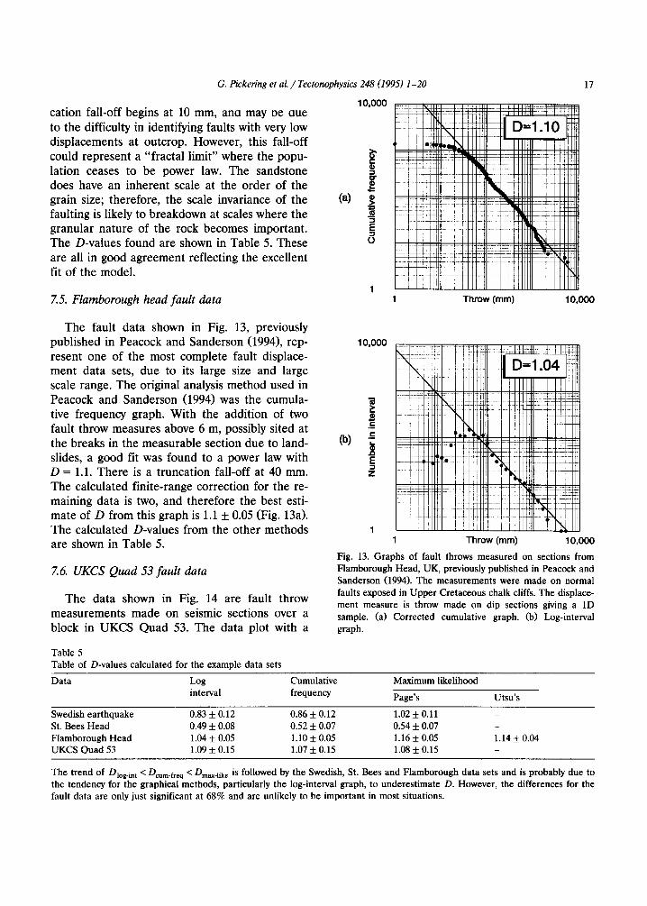
7.5. Flamborough head fault data

1 0 , 0 0 0

e -

- t

(a)

"5 E O

17

I ~ : ~ L : , ~ : I - ~ I 3 ~ F + ~ . . . . . . . . . . ,---T ....... l ' l l l l l l , , [ ' , I I ' , I I 7 , , ', ' , l ' , ' , l l i , - - - ,

- i i l l l l l =

IIIIII I ' l l l t l t l t i I l'll]ll

1 Throw (mm) 10,000

T h e faul t d a t a shown in Fig. 13, previous ly pub l i shed in Peacock and Sande r son (1994), rep- r esen t one of the most c o m p l e t e faul t d isplace- m e n t d a t a sets, due to its large size and large scale range . The or ig ina l analysis m e t h o d used in Peacock and S a n d e r s o n (1994) was the cumula - tive f requency graph. W i t h the add i t i on of two faul t th row m e a s u r e s above 6 m, possibly s i ted at the b reaks in the m e a s u r a b l e sec t ion due to land- slides, a good fit was found to a power law with D = 1.1. T h e r e is a t runca t ion fal l-off at 40 mm. The ca l cu la t ed f in i te - range co r rec t ion for the re- ma in ing da t a is two, and the re fo re the bes t estima te of D f rom this g raph is 1.1 + 0.05 (Fig. 13a). T h e ca l cu la t ed D-va lues f rom the o t h e r m e t h o d s are shown in Tab le 5.

7.6. UKCS Quad 53 fault data

T h e da t a shown in Fig. 14 a re faul t th row m e a s u r e m e n t s m a d e on seismic sect ions over a b lock in U K C S Q u a d 53. The da t a p lo t with a

1 0 , 0 0 0

I- li"il ' ili i l D=1.04 HWI I I il i 11111 1 !lllllll I I!l/iit

(b) "E

z

1 Throw (mm) 10,000

Fig. 13. Graphs of fault throws measured on sections from Flamborough Head, UK, previously published in Peacock and Sanderson (1994). The measurements were made on normal faults exposed in Upper Cretaceous chalk cliffs. The displacement measure is throw made on dip sections giving a 1D sample. (a) Corrected cumulative graph. (b) Log-interval graph.

Table 5 Table of D-values calculated for the example data sets

Data Log Cumulative Maximum likelihood interval frequency Page's Utsu's

Swedish earthquake 0.83 + 0.12 0.86 + 0.12 1.02 + 0.11 - St. Bees Head 0.49 + 0.08 0.52 + 0.07 0.54 + 0.07 - Flamborough Head 1.04 + 0.05 1.10 + 0.05 1.16 + 0.05 1.14 + 0.04 UKCS Quad 53 1.09 + 0.15 1.07 + 0.15 1.08 + 0.15

The trend of Dlog.ln t < Dcum.freq < Dmax_like is followed by the Swedish, St. Bees and Flamborough data sets and is probably due to the tendency for the graphical methods, particularly the log-interval graph, to underestimate D. However, the differences for the fault data are only just significant at 68% and are unlikely to be important in most situations.


distinct curve on the uncorrected cumulative graph (Fig. 14a), which would be expected given a truncation fall-off as the seismic resolution is approached and a significant finite-range effect. However, the data also fit the log-normal model (Fig. 14b). As the scale range of the data is so narrow, the decision on the most appropriate model must be based on additional criteria. There are two good reasons for fitting to a power-law model. Firstly, it is quite clear from the examples shown earlier and many other published data (e.g., Kakimi, 1980; Childs et al., 1990; Walsh et al., 1991, 1994; Jackson and Sanderson, 1992; Pickering et al., 1994) that fault populations in

many different areas are power-law distributed. Secondly, the fit to the log normal is only good if there is no increase in fault density below the scale range of the data. Faulting occurs on scales at least down to millimetres and there is good evidence that this faulting may be of sufficient density to follow the same power law as the large-scale data (Walsh et al., 1991; Jackson and Sanderson, 1992; Marrett and Allmendinger, 1992; Pickering et al., 1994). The fit to the log- normal model is almost certainly caused by the truncations of the data and the power-law model is a better for the population as a whole. The calculated D-values from the corrected cumula-

(a)

1 0 0 0

o>, - - ~ _ _ _ ~ _ _ ~ L _ * i

i l

~r I i ̧ ' ' i ,I

E

1 0.001

i J , ,

Throw (s) 1

(b)

99

95

68

s o ® .-> 32

E (9

5

1

0 . 0 0 1

i ~ = i i ! l l i

i i i i ~ ~ ! i ! !MII

Throw (s) 1

(c)

1000 - - - ~ i ' '

! ! i i l ]

:°°2 =, E :

0

1 0.001 Throw (s) 1

1 0 0 0 . . . . . . . . . . ~ i ' :

~ ~ 1 D = 1 . 0 7 ~ k ! i!

"~\ i i I : ! i l i j

* i ~ j i JO i j ~ [ I ~ ' , I E ~--~ : i i r N I il2!il

~ i I I ' '

: i , , i!i 1 ' , ~,ii:! i :l i

0.001 Th row (s) 1

Fig. 14. Graphs of fault throw data derived from UKCS Quad 53. The measurements were made at the Base Zechstein horizon in the Permian, picked on migrated sections of good quality. The sections were all dip lines giving a 1D sample. (a) Uncorrec ted cumulative frequency. (b) Log-normal probability plot (see Fig. 10b). (c) Corrected cumulative frequency graph. (d) Log-interval graph.


tive graph (Fig. 14c), the log-interval graph (Fig. 14d) and Page's maximum likelihood method are shown in Table 5. The narrow scale range reduces the chance of bias, but leads to an increase in uncertainty, reflected in the wide confidence interval.

8. Conclusions

(1) The three commonly used definitions of the power-law distribution are compatible but not equivalent. The cumulative frequency definition is preferred as it is consistent with the two alternative definitions and embodies the hierarchial nature of the power law.

(2) All data held to be power-law distributed represent samples from some underlying population. As these samples often cover a narrower scale range than that of the population as a whole they are truncated, and any analysis must recog- nise and allow for this.

(3) In some cases the samples may be censored, have a truncation "fall-off" or contain other additional sources of bias, that must be resolved before the data are analysed.

(4)Truncated data can be analysed by several methods: (a) cumulative frequency graphs; (b) discrete frequency graphs; (c) log-interval discrete frequency graph; and (d) maximum likelihood formulations. All of the methods are in some degree affected by the truncation of the data. The cumulative graph often gives biased D-values and appears to show deviations from a power-law distribution solely due to the scale range limitations of the data. This "finite-range" effect can be corrected and a procedure is outlined which is generally effective. The discrete frequency graph and log-interval graph are not affected by this bias and can be used as long as those intervals which straddle the truncation are ignored. Of the two commonly used maximum likelihood formulations, Utsu's approximate form is only suitable for data with a wide scale range ( > two orders of magnitude). Page's formulation, which was developed for truncated data, can be applied in all cases.

(5) These methods were tested by making a

Monte Carlo simulation of the sampling and analysis process. The results of the simulations gave an empirical relationship between the confidence intervals, sample size and D-value, with a constant term (k) controlled by the scale range of the sample and the method of analysis.

(6) The corrected cumulative graph, log-interval graph and Page's maximum likelihood method gave minimal bias and similar values for k. The discrete graph was rejected as it produced biased results with values of k two or three times those given by the other methods.

(7) Sub-samples from large earthquake magnitude and fault throw data sets showed sample D-value distributions equivalent to the simulated distributions, giving added confidence in the re- suits of the simulations.

(8) The proper consideration of sampling effects and selection of analysis methods can give consistent results, as illustrated by analysing several published and unpublished data sets.

Acknowledgements

The authors wish to thank David Peacock for access to the fault data from St. Bees Head and Flamborough Head, and his help with the Har- vard CMT catalogue. The authors also wish to thank Seismograph Service Ltd. and SHELF for permission to use the SSL-MF89 survey. Con- structive reviews by Patience Cowie, Michael Gross and Chris Scholz helped to improve the final version. This research is funded by a stu- dentship from Mobil North Sea Ltd.

References

Aki, K., 1965. Maximum likelihood estimate of b in the formula log N = a - brn and its confidence limits. Bull. Earthquake Res. Inst., Tokyo Univ., 43: 237-239.

Barton, C.A. and Zoback, M.D., 1992. Self similar distribution and properties of macroscopic fractures at depth in crys- talline rock in the Cajon Pass Scientific borehole. J. Geo- phys. Res., 97: 5181-5200.

Bath, M., 1979. Earthquakes in Sweden 1951-1976. Swed. Geol. Surv. NTIS, C 750.

Bath, M., 1981. Earthquake magnitude --recent research and current trends. Earth-Sci. Rev., 17: 315-398.


Bender, B., 1983. Maximum likelihood estimation of b values for magnitude grouped data. Bull. Seismol. Soc. Am., 73: 831-85 i.

Childs, C., Walsh, J.J. and Watterson, J., 1990. A method for estimation of the density of fault displacements below the limits of seismic resolution in reservoir formations. In: A.T. Buller (Editor), North Sea Oil and Gas Reservoirs II. Graham and Trotman, London, pp. 309-318.

Cruden, D.M., 1977. Describing the size of discontinuities. Int. J. Rock Mech. Min. Sci. Geomech. Abstr., 14: 133-137.

Einstein, H.H. and Baecher, G.B., 1983. Probabilistic and statistical methods in engineering geology, specific methods and examples Part I: Exploration. Rock Mech. Rock Eng., 16: 39-72.

Frochlich, C. and Davis, S.D., 1993. Teleseismic b values: or much ado about 1.0. J. Geophys. Res., 98: 631-644.

Gutenberg, B. and Richter, C.F., 1954. Seismicity of the Earth and Associated Phenomena (2nd ed.). Princetown Univ. Press, Princetown, NJ.

Heifer, K. and Bevan, T., 1990. Scaling relationships in natu- ral fractures-data, theory and applications. Proc. Eur. Petrol. Conf., 2:367-376 (SPE Pap. 20981).

Jackson, P. and Sanderson, D.J., 1992. Scaling of fault displacements from the Badajoz Cordoba shear zone, SW Spain. Tectonophysics, 210: 179-190.

Kakimi, T., 1980. Magnitude frequency relation for displacement of minor faults and its significance in crustal defor- mation. Bull. Geol. Soc. Jpn., 31: 467-487.

Laslett, G.M., 1982. Censoring and edge effects in areal and line transect sampling of rock joint traces. Math. Geol.. 14: 125-140.

Marrett, R. and Allmendinger, R.W., 1991. Estimates of strain due to brittle faulting: sampling of fault populations. J. Struct. Geol., 13: 735-738.

Marrett, R. and Allmendinger, R.W., 1992. Amount of extension on "small" faults: An example from the Viking graben. Geology, 20: 47-50.

Nelson, W. and Hahn, G.J., 1972. Linear estimation of a regression relationship from censored data - -Part I. Sim- ple methods and their application. Technometrics, 14: 247-269.

Nelson, W. and Hahn, G.J., 1973. Linear estimation of a regression relationship from censored data - -Part I1. Best linear unbiased estimation and theory. Technometrics, 15: 133-150.

Pacheco, J.F., Scholz, C.H. and Sykes, L.R., 1992. Changes in

frequency-size relationship from small to large earthquakes. Nature, 355: 71-73.

Page, R., 1968. Aftershocks and microaftershocks of the Great Alaska earthquake of 1964. Bull. Seismol. Soc. Am., 58: 1131-1168.

Peacock, D.C.P. and Sanderson, D.J., 1994. Strain and scaling of faults in the chalk at Flamborough Head, U.K.J. Struct. Geol., 16: 97-107.

Pickering, G., Bull, J.M., Sanderson, D.J. and Harrison, P.V., 1994. Fractal fault displacements: A case study from the Moray Firth, Scotland. In: J.H. Kruhl (Editor), Fractals and Dynamic Systems in Geosciences. Springer-Verlag, Berlin, pp. 105-120.

Pickering, G., Bull, J.M. and Sanderson, D.J., in press. Scaling of fault displacements and implications for the estimation of sub-seismic strain. In: P. Buchanan and D.A. Nieuw- land (Editors), Modern Developments in Structural Inter- pretation. Spec. Publ. Geol. Soc. London.

Press, W.H., Flannery, B.P., Teukolsky, S.A. and Vetterling, W.T., 1986. Numerical Recipes: The Art of Scientific Computing. Cambridge Univ. Press, Cambridge.

Priest, S.D. and Hudson, J.A., 1981. Estimation of discontinu- ity spacing and trace length using scanline surveys. Int. J. Rock Mech. Min. Sci. Geomech. Abstr., 18: 183-197.

Rubinstein, R.Y., 1981. Simulation and the Monte Carlo Method. Wiley, New York, NY.

Schroeder, M., 1991. Fractals, Chaos, Power-laws: Minutes from a Infinite Paradise. Freeman, New York.

Utsu, T., 1965. A method for determining the value of b in a formula log n = a - bM showing the magnitude-frequency relation for earthquakes. Geophys. Bull. Hokkaido Univ., 13: 99-103.

Walsh, J.J. and Watterson, J., 1988. Analysis of the relationship between displacements and dimensions of faults. J. Struct. Geol., 10: 239-247.

Walsh, J.J., Watterson, J. and Yielding, G., 1991. The impor- tance of small scale faulting in regional extension. Nature, 351: 391-393.

Walsh, J.J., Watterson, J. and Yielding, G., 1994. Determina- tion and interpretation of fault size populations: procedures and problems. In: North Sea Oil and Gas Reservoirs --III . Norw. Inst. Technol., pp. 141-155.

Yielding, G., Walsh, J.J. and Watterson, J., 1992. The prediction of small-scale faulting in reservoirs. First Break, 10: 449-460.

sampling power-law distributions - eprintseprints.soton.ac.uk/40880/1/pickeringetal.pdf ·...

Documents