sampling method for 2d/3d building plans derived from 3d

1

Evaluation of an Acceptance Sampling Method for 2D/3D Building Plans Derived from 3D Imaging Data

Geraldine Cheok1, Marek Franaszek1, and James Filliben1

Abstract

An acceptance sampling method, based on obtaining physical measurements, for accepting 2D building plans generated from 3D imaging data is evaluated and demonstrated using an actual GSA (General Services Administration) facility. The objective of the effort was to determine practical/feasible limits for the tolerances (T), sample size (n), and the maximum percent of the population (P) out‐of‐spec that is acceptable for GSA. A total of 285 measurements were obtained from a GSA 3D imaging project site by the National Institute of Standards and Technology (NIST) and Carnegie Mellon University (CMU). These measurements were then compared to corresponding measurements extracted from 2D plans or 3D models. Several thousands of simulations were run for different combinations of samples (i.e., to randomize the data sampling) for a given set of n, P, and T. The data collection, data analysis, and findings are presented in this paper. Keywords: 3D imaging; acceptance sampling; 2D building plans; 3D model; quality assurance.

1 Introduction

The use of and applications for 3D imaging systems (e.g., laser scanners) have grown tremendously in the past decade. With this growth, there has been an increasing number of studies to evaluate the performance of and to calibrate these systems (e.g., [1‐6]). To a lesser extent, there have been efforts to develop best practices to minimize the sensor errors [1, 7] and to evaluate the end products derived from 3D imaging data such as 2D building plans or 3D models [8]. These efforts provide important information on the sensor performance and are required to enable propagation of the sensor errors and to enable development of standards for 3D imaging systems. Currently, there no standards or guidelines for 3D imaging systems although there are on‐going efforts (e.g., ASTM E57 – 3D Imaging Systems, VDI/VDE2) to do so. However, in the interim, users of 3D imaging technology have been developing their own procedures. One such user is the U.S. General Services Administration (GSA).

Specifically, GSA is investigating the use of 3D imaging technologies to capture existing conditions of government facilities. GSA has been involved in developing guidance for their project managers to assess the application of 3D imaging in GSA projects. As a part of this effort, GSA contracted the National Institute of Standards and Technology (NIST) to contribute to the development of the guidance documents. This collaboration resulted in the publication of:

1 National Institute of Standards and Technology, 100 Bureau Drive, MS 8611, Gaithersburg, MD, 20899‐8611. [email protected] (corresponding author), marek. [email protected], [email protected].

2 German committee: VDI/VDE – Society Measurement and Automation

2

• Phase I and II ‐ “BIM Guide for 3D Imaging” [9]. This document provides a general introduction to and guidance for 3D imaging to GSA project managers.

• Phase II ‐ “Guidelines for Accepting 2D Building Plans” [10]. The objective of this document is to aid GSA in the objective assessment of the deliverables from 3D imaging data – in particular, 2D building plans. The guideline provides a systematic answer to the question:

Are the dimensional deviations from the derived 2D plans within the specifications stated in the contract?

This method utilizes Acceptance Sampling to either accept or reject a 2D building plan. The method involves several steps as briefly described below:

1. Determine measurement type that is important (e.g., room dimensions, pipe diameters) 2. Specify how the measurements are to be made 3. Specify criteria for conformity of measurement ‐ when the measurement is “in‐spec” or “out‐

of‐spec”. 4. Define tolerance, T, maximum tolerable percent of the population out‐of‐spec, P, and

sample size, n 5. Determine which measurements to be obtained 6. Obtain measurements 7. Analyze the data – determine number of defects or out‐of‐spec 8. Accept/Reject 2D building plan using “Upper Limit Table on % Defective in Population.”

In Phase III, the focus is on evaluating and demonstrating the acceptance sampling procedure developed from Phase II using an actual GSA facility. In particular, the objective is to determine practical/feasible limits for T, n, and P where:

• T, tolerance, is the maximum deviation that a measurement could have before the measurement is declared to be "out‐of‐spec". Deviation = |2D/3D measurement – reference value|.

• P is the maximum percent of the population that is out‐of‐spec that is acceptable to the facility owner.

• n is the number of measurements that will be made by an inspector; statistically, n is referred to as the "sample size". This number will depend largely on time and cost expended to perform the quality check.

To accomplish the objective, it was necessary to obtain field measurements from a facility and then comparing these measurements to corresponding measurements extracted from 2D plans or 3D models. Several thousands of simulations were run for different combinations of samples (i.e., to randomize the data sampling) for a given set of n, P, and T. A summary of the data collection, data analysis, and findings are presented in this paper (see [11] for details).

At this time, there is no guidance on what are appropriate values for T, n, P, i.e., what is feasible or practical. The effort described in this paper will provide initial guidance to the questions: 1) How many

3

measurements are needed? 2) What is an acceptable percent of out‐of‐spec? 3) What is a practical tolerance?

2 Data Collection

2.1 Facility Description

A GSA 3D imaging project was used to help evaluate practical/feasible values for T, P, and n. The facility is a utility plant which provides electricity and hot water for several buildings. The rooms in the facility could be categorized as either offices or mechanical equipment rooms.

One of the objectives of the GSA 3D imaging project was to obtain a record of existing building conditions. The primary use of the data is for verification and comparison of the spatial data and area measurements. The GSA specified tolerance for the deliverables from the service provider for all of the measurements that will be used in this report is 25.4 mm.

2.2 Manual Data Collection

The measurements of interest to GSA were interior room dimensions. GSA was also interested, to a lesser extent, in pipe dimensions, equipment dimensions, and exterior dimensions.

2.2.1 1st Data Collection

In February, 2009, NIST researchers collected the data to be compared with the measurements from the 2D plans or 3D model (2D/3D measurements will be used henceforth) at the same time that the service provider was scanning the facility. A team of researchers from Carnegie Mellon University (CMU) was also at the site collecting measurements for a related GSA project. The types of measurements obtained were: room dimensions (width and height), window widths and heights, distance between objects (e.g., columns, equipment and wall), pipe diameters, and pipe circumferences. Two hundred and forty‐two (242) measurements were obtained from the interior and exterior of the building and on the roof.

For the majority of the 242 measurements, the measurement was repeated where the number of repeats varied from two to eight. To clarify, a measurement is the average of the repeated measurements of the dimension of interest. For example, if the dimension of interest was a door width, the door width was measured three times: near the top of the door, middle of the door, close to the bottom of the door. The average of these three measurements was used to represent the NIST/CMU measurement for that door width; this constitutes one of the 242 measurements – NOT three of the 242 measurements.

2.2.1.1 Comparison of Manual Measurements

The CMU data were made available to NIST and vice versa. Of the 242 NIST measurements, there were a total of 15 corresponding measurements in the CMU data set, i.e, NIST and CMU obtained 15 measurements of the same dimension.

The differences for 14 of the 15 measurements were less than 6 mm. The average of the absolute values of the differences (without the outlier) was 3.2 mm with a standard deviation of 1.9 mm. There

4

were 29 other measurements from CMU that did not duplicate any of the NIST measurements, and these 29 measurements were combined with the NIST measurements.

2.2.2 2nd Data Collection

After an initial analysis of the data, there were 30 measurements where the difference between the NIST or CMU measurements and the extracted measurements from the 2D plans or 3D model was more than 50.8 mm. To verify the manual measurement values, NIST re‐visited the site in October, 2009 and re‐measured the 30 dimensions. Five of the 30 measurements could not be obtained.

Of the 25 measurements that were repeated, 23 were essentially the same as the data collected in the 1st data collection. In addition to obtaining the 25 repeated measurements, 31 additional measurements were made to augment the number of measurements obtained in the 1st data collection.

2.2.3 Data Description

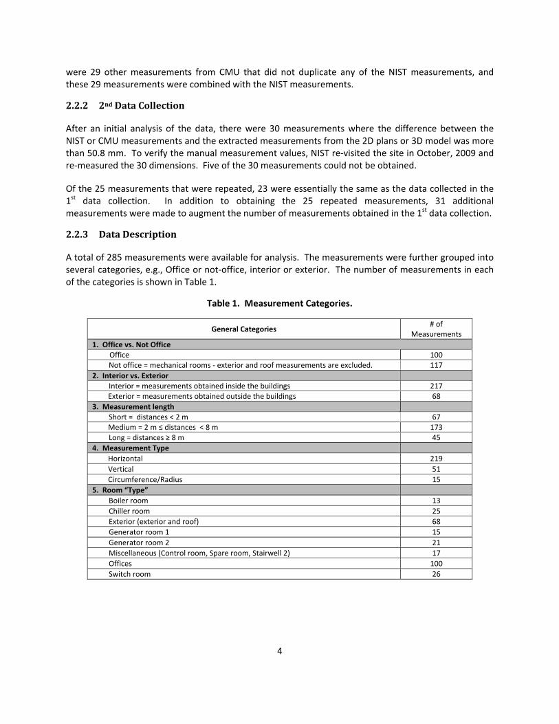
A total of 285 measurements were available for analysis. The measurements were further grouped into several categories, e.g., Office or not‐office, interior or exterior. The number of measurements in each of the categories is shown in Table 1.

Table 1. Measurement Categories.

General Categories # of

Measurements 1. Office vs. Not Office Office 100

Not office = mechanical rooms ‐ exterior and roof measurements are excluded. 117 2. Interior vs. Exterior Interior = measurements obtained inside the buildings 217 Exterior = measurements obtained outside the buildings 68 3. Measurement length Short = distances < 2 m 67 Medium = 2 m ≤ distances < 8 m 173 Long = distances ≥ 8 m 45 4. Measurement Type Horizontal 219 Vertical 51 Circumference/Radius 15 5. Room “Type” Boiler room 13 Chiller room 25 Exterior (exterior and roof) 68 Generator room 1 15 Generator room 2 21 Miscellaneous (Control room, Spare room, Stairwell 2) 17 Offices 100 Switch room 26

5

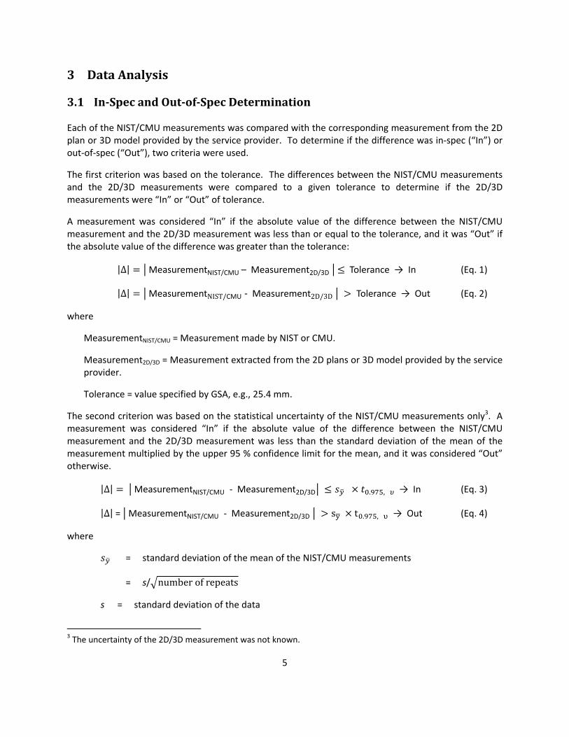
3 Data Analysis 3.1 InSpec and OutofSpec Determination Each of the NIST/CMU measurements was compared with the corresponding measurement from the 2D plan or 3D model provided by the service provider. To determine if the difference was in‐spec (“In”) or out‐of‐spec (“Out”), two criteria were used.

The first criterion was based on the tolerance. The differences between the NIST/CMU measurements and the 2D/3D measurements were compared to a given tolerance to determine if the 2D/3D measurements were “In” or “Out” of tolerance.

A measurement was considered “In” if the absolute value of the difference between the NIST/CMU measurement and the 2D/3D measurement was less than or equal to the tolerance, and it was “Out” if the absolute value of the difference was greater than the tolerance:

|Δ| MeasurementNIST/CMU – Measurement2D/3D Tolerance → In (Eq. 1)

|Δ| MeasurementNIST/CMU ‐ Measurement2D/3D Tolerance → Out (Eq. 2)

where

MeasurementNIST/CMU = Measurement made by NIST or CMU.

Measurement2D/3D = Measurement extracted from the 2D plans or 3D model provided by the service provider.

Tolerance = value specified by GSA, e.g., 25.4 mm.

The second criterion was based on the statistical uncertainty of the NIST/CMU measurements only3. A measurement was considered “In” if the absolute value of the difference between the NIST/CMU measurement and the 2D/3D measurement was less than the standard deviation of the mean of the measurement multiplied by the upper 95 % confidence limit for the mean, and it was considered “Out” otherwise.

|Δ| MeasurementNIST/CMU ‐ Measurement2D/3D . , → In (Eq. 3)

|Δ| = MeasurementNIST/CMU ‐ Measurement2D/3D s t . , → Out (Eq. 4)

where

= standard deviation of the mean of the NIST/CMU measurements

= s/ number of repeats

s = standard deviation of the data

3 The uncertainty of the 2D/3D measurement was not known.

6

= mean of the data

. , = 97.5 % percentile of a two‐sided t‐distribution with υ degrees of freedom.

υ = number of repeats – 1

If the decision is “In” based on one criteria and “Out” based on the other criteria, the final decision is “In”. Therefore, the only time when the final decision is to Reject is when the decision is Reject for both criteria.

3.2 Influence of n, T, P, and Sampling Strategy on the Decision

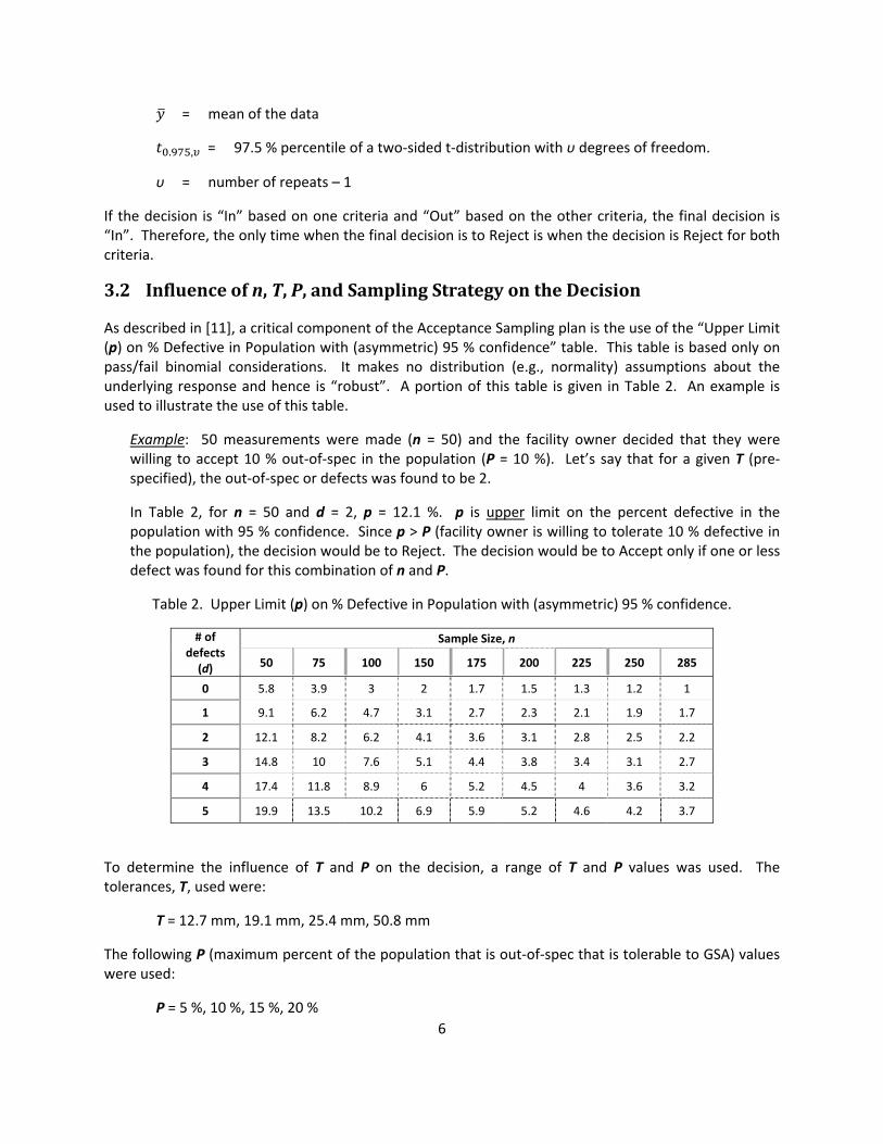
As described in [11], a critical component of the Acceptance Sampling plan is the use of the “Upper Limit (p) on % Defective in Population with (asymmetric) 95 % confidence” table. This table is based only on pass/fail binomial considerations. It makes no distribution (e.g., normality) assumptions about the underlying response and hence is “robust”. A portion of this table is given in Table 2. An example is used to illustrate the use of this table.

Example: 50 measurements were made (n = 50) and the facility owner decided that they were willing to accept 10 % out‐of‐spec in the population (P = 10 %). Let’s say that for a given T (pre‐specified), the out‐of‐spec or defects was found to be 2.

In Table 2, for n = 50 and d = 2, p = 12.1 %. p is upper limit on the percent defective in the population with 95 % confidence. Since p > P (facility owner is willing to tolerate 10 % defective in the population), the decision would be to Reject. The decision would be to Accept only if one or less defect was found for this combination of n and P.

Table 2. Upper Limit (p) on % Defective in Population with (asymmetric) 95 % confidence.

# of defects (d)

Sample Size, n

50 75 100 150 175 200 225 250 285

0 5.8 3.9 3 2 1.7 1.5 1.3 1.2 1

1 9.1 6.2 4.7 3.1 2.7 2.3 2.1 1.9 1.7

2 12.1 8.2 6.2 4.1 3.6 3.1 2.8 2.5 2.2

3 14.8 10 7.6 5.1 4.4 3.8 3.4 3.1 2.7

4 17.4 11.8 8.9 6 5.2 4.5 4 3.6 3.2

5 19.9 13.5 10.2 6.9 5.9 5.2 4.6 4.2 3.7

To determine the influence of T and P on the decision, a range of T and P values was used. The tolerances, T, used were:

T = 12.7 mm, 19.1 mm, 25.4 mm, 50.8 mm

The following P (maximum percent of the population that is out‐of‐spec that is tolerable to GSA) values were used:

P = 5 %, 10 %, 15 %, 20 %

7

For given combinations of T and P, eight sampling strategies were implemented to evaluate the effect of sample size, n. Since only “one” large sample set (N = 285) was obtained in the field, the effect of varying the sample size was simulated by sub‐sampling from the “one” large sample set. The sub‐sampling (taking n measurements from N where n < N) enables the randomization of the selection of the measurements. For a sub‐sample size of n, the number of all possible combinations out of N samples is:

!

! ! (Eq. 5)

The eight sampling strategies are described below.

1. All measurements (M=285 measurements available)

This sampling method is the Randomized Acceptance Sampling method where all the measurements are selected randomly. Sample sizes used: n = 50, 75, 100, 125, 150, 175, 200, 225, 250, 285.

2. All Offices only (M=100 measurements available)

This sampling method is the Randomized Acceptance Sampling method for offices only. This strategy allows for the simulation of projects where the building(s) consisted of office spaces only. Sample sizes used: n = 50, 75, 100.

3. All Not Offices only (M=117 measurements available)

This sampling method is the Randomized Acceptance Sampling method for not offices only. This strategy allows for the simulation of projects where the buildings did not contain office spaces and where the environment was less structured. Sample sizes used: n = 50, 75, 100, 117.

4. Equal number of measurements for each room type (Table 1, General Category 5)

This sampling method is the Stratified Randomized Acceptance Sampling. The stratification is based on room type. Eight room types used were: Boiler room, Chiller room, Exterior, Generator room 1, Generator room 2, Miscellaneous, Office, Switch room.

Sample sizes used: n = 8*k = 8*6 = 48 (for k = 6 measurements/ room type), 64 (for k =8), 80 (for k = 10), 104 (for k = 13). Randomly select k measurements within a room type 200 times for each n.

5. Offices or Not Offices (Table 1, General Category 1, M=217)

This sampling method is the Stratified Randomized Acceptance Sampling. The stratification is based on whether the measurement was from an Office space (more structured environment) or Not Office space (less structured environment). Sample sizes used: n = 50, 75, 100, 125, 150, 175, 200, 217. The ratio of office to not office measurements was kept constant when selecting the n samples.

6. Interior or Exterior (Table 1, General Category 2, M=285)

8

This sampling method is the Stratified Randomized Acceptance Sampling. The stratification is based on whether the measurement was an Interior or Exterior measurement. Sample sizes used: n = 50, 75, 100, 125, 150, 175, 200, 225, 250, 285. The ratio of interior to exterior measurements was kept constant when selecting the n samples.

7. Measurement length (Table 1, General Category 3, M= 285)

This sampling method is the Stratified Randomized Acceptance Sampling. The stratification is based on measurement length (short, medium, long). Sample sizes used: n = 50, 75, 100, 125, 150, 175, 200, 225, 250, 285. The relative proportions of the three categories were kept constant when selecting the n samples.

8. Measurement Type (Table 1, General Category 4,M=270)

This sampling method is the Stratified Randomized Acceptance Sampling. The stratification is based on measurement type – horizontal vs. vertical. Sample sizes used: n = 50, 75, 100, 125, 150, 175, 200, 225, 250, 270. The ratio of horizontal to vertical measurements was kept constant when selecting the n samples.

Except for Strategy 4, for each n (except for n = M), randomly select measurements 400 times out of the M available measurements. Comparisons of Strategy 1 with Strategies 4 to 8 will allow for the comparison of randomized sampling versus stratified randomized acceptance sampling described in [11].

4 Results and Discussion During the study, two sources that potentially contributed to the out‐of‐spec measurements were identified. One source was the way that the data was collected which affected the measurements of the floor to ceiling distances in the “Not Office” areas. There were eight such measurements. All floor‐to‐ceiling measurements (“Not Office” and “Office”) were obtained from three locations around the room, and the average of the measurements at the three locations was used to compare with the 2D/3D measurement. The ceilings in the “Not Office” areas were sloped, and this slope may have caused some of the floor‐to‐ceiling measurements in the “Not Office” areas to be out‐of‐spec. Of the eight measurements, there were five instances when the floor‐to‐ceiling measurements in the “Not Office” areas were out‐of‐spec.

The other source was the simplification used when creating the 2D/3D model. This affected measurements of windows where the window had different interior and exterior faces but the model did not. There were 14 such measurements. The 3D model was generated using the points for the exterior face of the window. Two of the 14 measurements were in‐spec for T ≥ 12.7 mm. For six of 14 measurements, the corresponding measurements from the point cloud (i.e., not from the model) were obtained from the service provider. Using the point cloud measurements, four of the six measurements would be in‐spec for T = 12.7 mm and all six would be in‐spec for T = 50.8 mm. However, to be consistent with the other extracted measurements, the 14 measurements extracted from the 2D/3D model were used in the analyses. That is, the measurements as extracted from the point clouds (obtained from the service provider) were not used.

9

4.1 General Findings

Table 3 categorizes the measurements based on the magnitude of the differences between the NIST/CMU measurements and the 2D/3D measurements.

Table 3. Magnitude of Differences between the Manual and 2D/3D Measurements.

Difference, D (mm)

# of Measurements

% of Measurements

D ≤ 12.7 193 68

12.7 < D ≤ 19.1 31 11

19.1 < D ≤ 25.4 20 7

25.4 < D ≤ 50.8 22 8

50.8 < D ≤ 76.2 7 2

76.2 < D ≤ 101.6 3 1

101.6 < D ≤ 127.0 3 1

D > 127.0 6 2

As shown in Table 3, the difference between the NIST/CMU and the 2D/3D plans for 68 % of the measurements was less than or equal to 12.7 mm and for 86 % of the measurements, the difference was 25.4 mm or less.

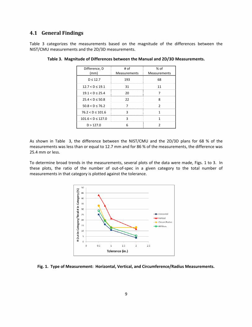
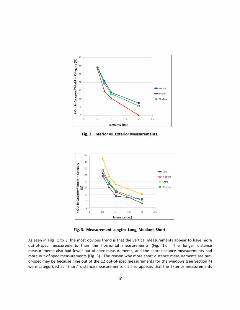
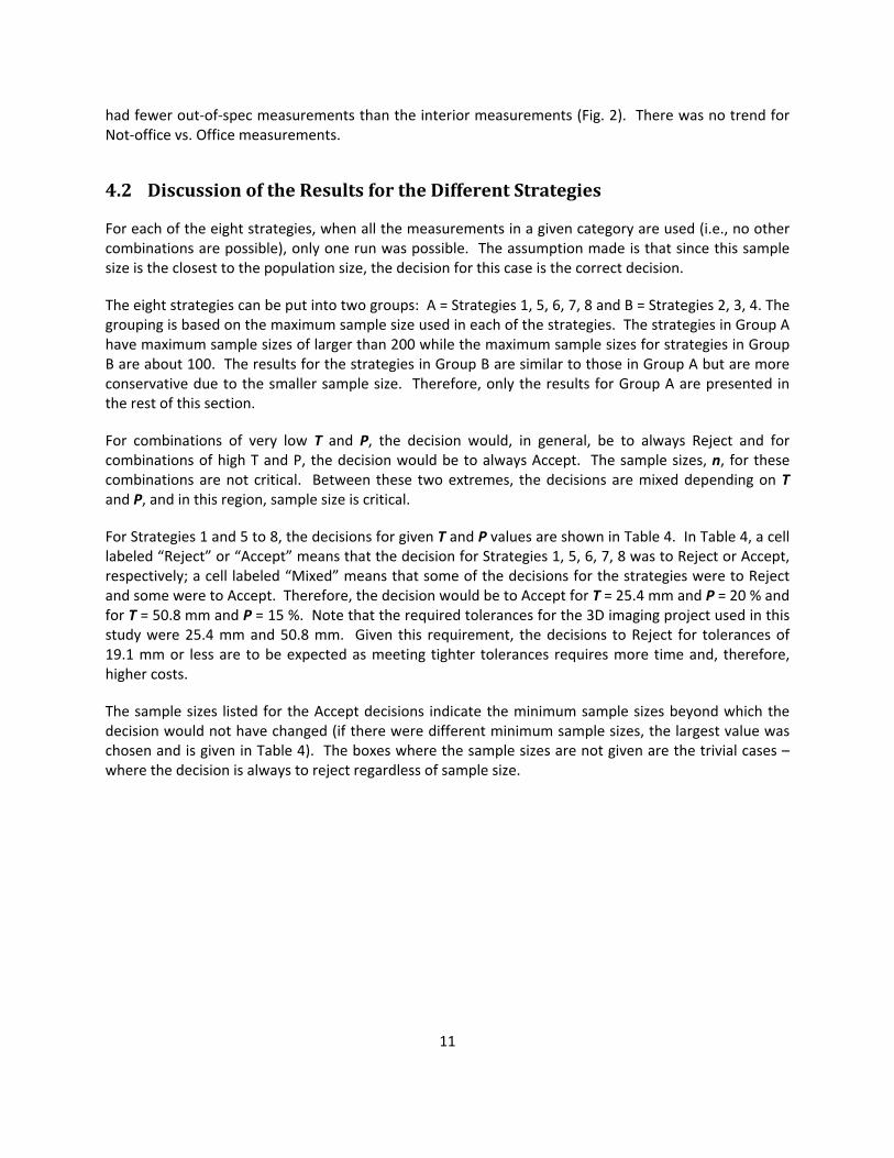
To determine broad trends in the measurements, several plots of the data were made, Figs. 1 to 3. In these plots, the ratio of the number of out‐of‐spec in a given category to the total number of measurements in that category is plotted against the tolerance.

Fig. 1. Type of Measurement: Horizontal, Vertical, and Circumference/Radius Measurements.

10

Fig. 2. Interior vs. Exterior Measurements.

Fig. 3. Measurement Length: Long, Medium, Short. As seen in Figs. 1 to 3, the most obvious trend is that the vertical measurements appear to have more out‐of‐spec measurements than the horizontal measurements (Fig. 1). The longer distance measurements also had fewer out‐of‐spec measurements, and the short distance measurements had more out‐of‐spec measurements (Fig. 3). The reason why more short distance measurements are out‐of‐spec may be because nine out of the 12 out‐of‐spec measurements for the windows (see Section 4) were categorized as “Short” distance measurements. It also appears that the Exterior measurements

11

had fewer out‐of‐spec measurements than the interior measurements (Fig. 2). There was no trend for Not‐office vs. Office measurements.

4.2 Discussion of the Results for the Different Strategies

For each of the eight strategies, when all the measurements in a given category are used (i.e., no other combinations are possible), only one run was possible. The assumption made is that since this sample size is the closest to the population size, the decision for this case is the correct decision.

The eight strategies can be put into two groups: A = Strategies 1, 5, 6, 7, 8 and B = Strategies 2, 3, 4. The grouping is based on the maximum sample size used in each of the strategies. The strategies in Group A have maximum sample sizes of larger than 200 while the maximum sample sizes for strategies in Group B are about 100. The results for the strategies in Group B are similar to those in Group A but are more conservative due to the smaller sample size. Therefore, only the results for Group A are presented in the rest of this section.

For combinations of very low T and P, the decision would, in general, be to always Reject and for combinations of high T and P, the decision would be to always Accept. The sample sizes, n, for these combinations are not critical. Between these two extremes, the decisions are mixed depending on T and P, and in this region, sample size is critical.

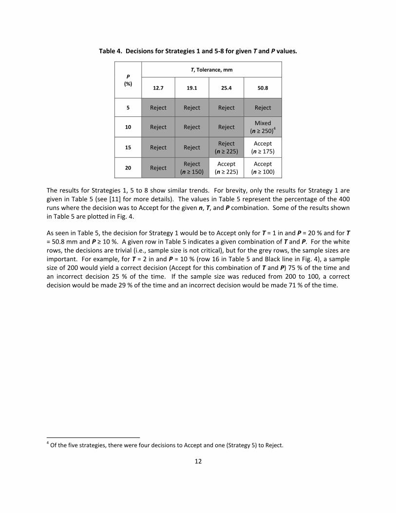
For Strategies 1 and 5 to 8, the decisions for given T and P values are shown in Table 4. In Table 4, a cell labeled “Reject” or “Accept” means that the decision for Strategies 1, 5, 6, 7, 8 was to Reject or Accept, respectively; a cell labeled “Mixed” means that some of the decisions for the strategies were to Reject and some were to Accept. Therefore, the decision would be to Accept for T = 25.4 mm and P = 20 % and for T = 50.8 mm and P = 15 %. Note that the required tolerances for the 3D imaging project used in this study were 25.4 mm and 50.8 mm. Given this requirement, the decisions to Reject for tolerances of 19.1 mm or less are to be expected as meeting tighter tolerances requires more time and, therefore, higher costs.

The sample sizes listed for the Accept decisions indicate the minimum sample sizes beyond which the decision would not have changed (if there were different minimum sample sizes, the largest value was chosen and is given in Table 4). The boxes where the sample sizes are not given are the trivial cases – where the decision is always to reject regardless of sample size.

12

Table 4. Decisions for Strategies 1 and 5‐8 for given T and P values.

P (%)

T, Tolerance, mm

12.7 19.1 25.4 50.8

5 Reject Reject Reject Reject

10 Reject Reject Reject Mixed

(n ≥ 250)4

15 Reject Reject Reject

(n ≥ 225) Accept (n ≥ 175)

20 Reject Reject

(n ≥ 150) Accept (n ≥ 225)

Accept (n ≥ 100)

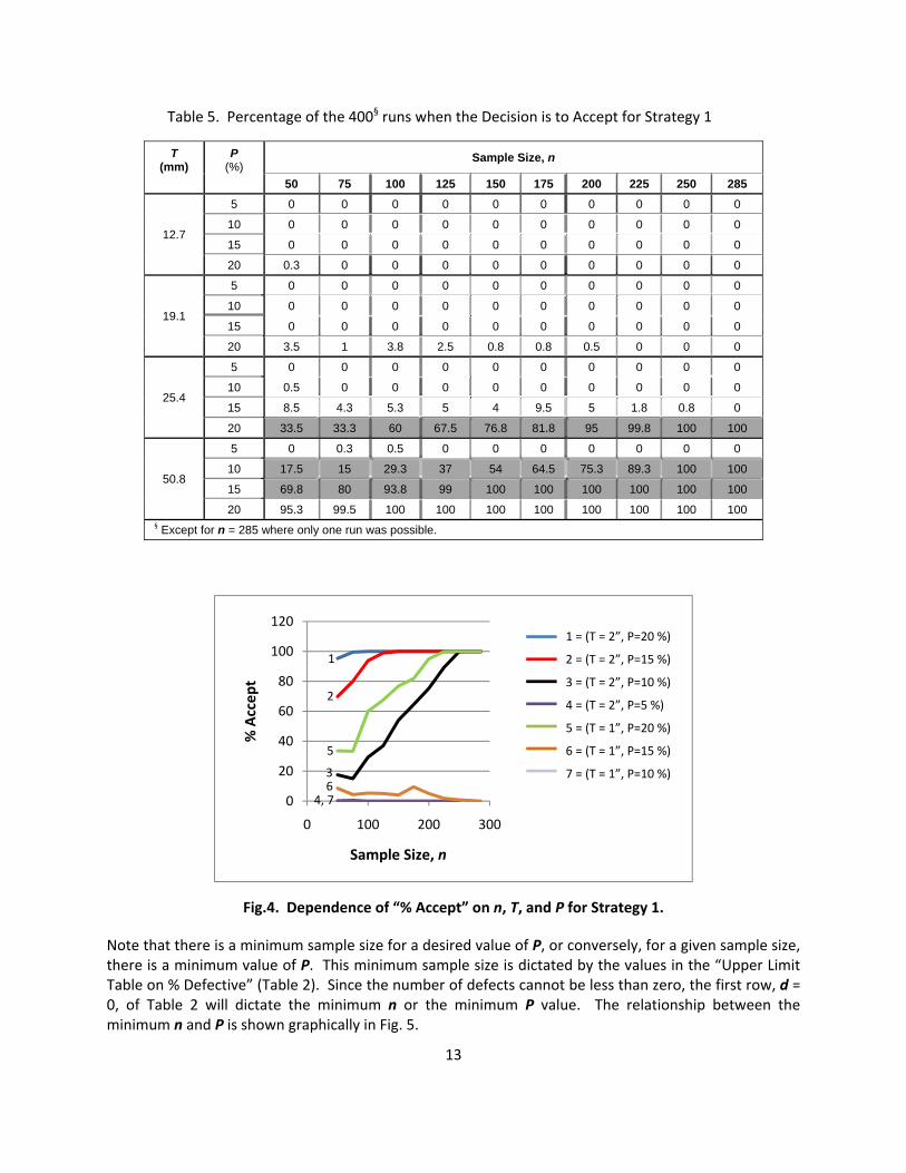
The results for Strategies 1, 5 to 8 show similar trends. For brevity, only the results for Strategy 1 are given in Table 5 (see [11] for more details). The values in Table 5 represent the percentage of the 400 runs where the decision was to Accept for the given n, T, and P combination. Some of the results shown in Table 5 are plotted in Fig. 4.

As seen in Table 5, the decision for Strategy 1 would be to Accept only for T = 1 in and P = 20 % and for T = 50.8 mm and P ≥ 10 %. A given row in Table 5 indicates a given combination of T and P. For the white rows, the decisions are trivial (i.e., sample size is not critical), but for the grey rows, the sample sizes are important. For example, for T = 2 in and P = 10 % (row 16 in Table 5 and Black line in Fig. 4), a sample size of 200 would yield a correct decision (Accept for this combination of T and P) 75 % of the time and an incorrect decision 25 % of the time. If the sample size was reduced from 200 to 100, a correct decision would be made 29 % of the time and an incorrect decision would be made 71 % of the time.

4 Of the five strategies, there were four decisions to Accept and one (Strategy 5) to Reject.

13

Table 5. Percentage of the 400§ runs when the Decision is to Accept for Strategy 1

T (mm)

P (%)

Sample Size, n

50 75 100 125 150 175 200 225 250 285

12.7

5 0 0 0 0 0 0 0 0 0 0

10 0 0 0 0 0 0 0 0 0 0

15 0 0 0 0 0 0 0 0 0 0

20 0.3 0 0 0 0 0 0 0 0 0

19.1

5 0 0 0 0 0 0 0 0 0 0

10 0 0 0 0 0 0 0 0 0 0

15 0 0 0 0 0 0 0 0 0 0

20 3.5 1 3.8 2.5 0.8 0.8 0.5 0 0 0

25.4

5 0 0 0 0 0 0 0 0 0 0

10 0.5 0 0 0 0 0 0 0 0 0

15 8.5 4.3 5.3 5 4 9.5 5 1.8 0.8 0

20 33.5 33.3 60 67.5 76.8 81.8 95 99.8 100 100

50.8

5 0 0.3 0.5 0 0 0 0 0 0 0

10 17.5 15 29.3 37 54 64.5 75.3 89.3 100 100

15 69.8 80 93.8 99 100 100 100 100 100 100

20 95.3 99.5 100 100 100 100 100 100 100 100 § Except for n = 285 where only one run was possible.

Fig.4. Dependence of “% Accept” on n, T, and P for Strategy 1.

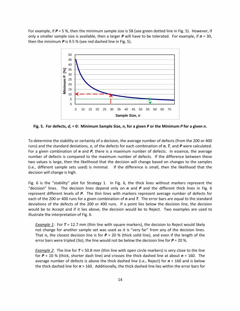
Note that there is a minimum sample size for a desired value of P, or conversely, for a given sample size, there is a minimum value of P. This minimum sample size is dictated by the values in the “Upper Limit Table on % Defective” (Table 2). Since the number of defects cannot be less than zero, the first row, d = 0, of Table 2 will dictate the minimum n or the minimum P value. The relationship between the minimum n and P is shown graphically in Fig. 5.

0

20

40

60

80

100

120

0 100 200 300

% Accep

t

Sample Size, n

1

2

5

3

1 = (T = 2”, P=20 %)

2 = (T = 2”, P=15 %)

3 = (T = 2”, P=10 %)

4 = (T = 2”, P=5 %)

5 = (T = 1”, P=20 %)

6 = (T = 1”, P=15 %)

7 = (T = 1”, P=10 %) 6

4, 7

14

For example, if P = 5 %, then the minimum sample size is 58 (see green dotted line in Fig. 5). However, if only a smaller sample size is available, then a larger P will have to be tolerated. For example, if n = 30, then the minimum P is 9.5 % (see red dashed line in Fig. 5).

Fig. 5. For defects, d, = 0: Minimum Sample Size, n, for a given P or the Minimum P for a given n.

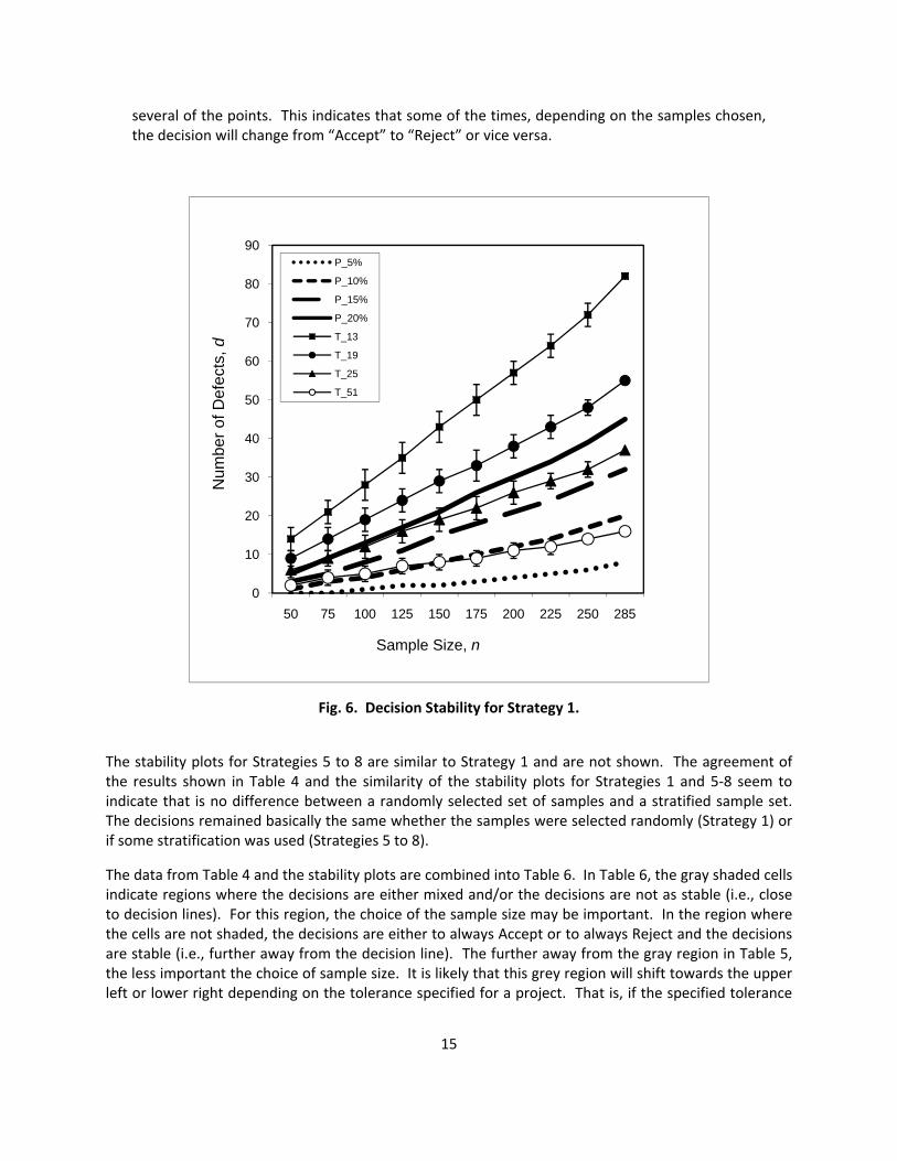
To determine the stability or certainty of a decision, the average number of defects (from the 200 or 400 runs) and the standard deviations, σ, of the defects for each combination of n, T, and P were calculated. For a given combination of n and P, there is a maximum number of defects. In essence, the average number of defects is compared to the maximum number of defects. If the difference between these two values is large, then the likelihood that the decision will change based on changes to the samples (i.e., different sample sets used) is minimal. If the difference is small, then the likelihood that the decision will change is high. Fig. 6 is the “stability” plot for Strategy 1. In Fig. 6, the thick lines without markers represent the “decision” lines. The decision lines depend only on n and P and the different thick lines in Fig. 6 represent different levels of P. The thin lines with markers represent average number of defects for each of the 200 or 400 runs for a given combination of n and T. The error bars are equal to the standard deviations of the defects of the 200 or 400 runs. If a point lies below the decision line, the decision would be to Accept and if it lies above, the decision would be to Reject. Two examples are used to illustrate the interpretation of Fig. 6.

Example 1: For T = 12.7 mm (thin line with square markers), the decision to Reject would likely not change for another sample set was used as it is “very far” from any of the decision lines. That is, the closest decision line is for P = 20 % (thick solid line), and even if the length of the error bars were tripled (3σ), the line would not be below the decision line for P = 20 %.

Example 2: The line for T = 50.8 mm (thin line with open circle markers) is very close to the line for P = 10 % (thick, shorter dash line) and crosses the thick dashed line at about n = 160. The average number of defects is above the thick dashed line (i.e., Reject) for n < 160 and is below the thick dashed line for n > 160. Additionally, the thick dashed line lies within the error bars for

05

101520253035404550

5 10 15 20 25 30 35 40 45 50 55 60 65 70

Min

imum

P [

%]

Sample Size, n

15

several of the points. This indicates that some of the times, depending on the samples chosen, the decision will change from “Accept” to “Reject” or vice versa.

Fig. 6. Decision Stability for Strategy 1.

The stability plots for Strategies 5 to 8 are similar to Strategy 1 and are not shown. The agreement of the results shown in Table 4 and the similarity of the stability plots for Strategies 1 and 5‐8 seem to indicate that is no difference between a randomly selected set of samples and a stratified sample set. The decisions remained basically the same whether the samples were selected randomly (Strategy 1) or if some stratification was used (Strategies 5 to 8).

The data from Table 4 and the stability plots are combined into Table 6. In Table 6, the gray shaded cells indicate regions where the decisions are either mixed and/or the decisions are not as stable (i.e., close to decision lines). For this region, the choice of the sample size may be important. In the region where the cells are not shaded, the decisions are either to always Accept or to always Reject and the decisions are stable (i.e., further away from the decision line). The further away from the gray region in Table 5, the less important the choice of sample size. It is likely that this grey region will shift towards the upper left or lower right depending on the tolerance specified for a project. That is, if the specified tolerance

0

10

20

30

40

50

60

70

80

90

50 75 100 125 150 175 200 225 250 285

Num

ber o

f Def

ects

, d

Sample Size, n

P_5%

P_10%

P_15%

P_20%

T_13

T_19

T_25

T_51

16

for a 3D imaging project is 19.1 mm, the service provider will try to meet this specification and the grey region will shift towards the upper left.

Table 6. Strategies 1 and 5‐8: General Trend for the Importance of Sample Size.

P (%)

T, Tolerance, mm

12.7 19.1 25.4 50.8

5 n not as critical

n not as critical

n not as critical

n not as critical

10 n not as critical

n not as critical

n not as critical

n important


n not as critical

n important

n important


n important

n important

n not as critical

5 Summary

A method using acceptance sampling to Accept or Reject 2D building plans/3D models was demonstrated using an actual 3D imaging project. The focus of this effort was to determine practical/feasible limits for the tolerances (T), sample size (n), and the maximum percent of the population (P) out‐of‐spec that is acceptable to a facility owner.

A total of 285 measurements were obtained from a GSA 3D imaging project site by NIST and CMU. Different types of measurements were made: horizontal, vertical, and non‐linear (e.g., circumference of pipes). These measurements were then compared to corresponding measurements extracted from 2D plans or 3D models.

Some possible sources of discrepancy between the manual and extracted 2D/3D measurements include:

1. Manual measurements a. Extraction of the incorrect dimension from 2D/3D model b. Incorrect measurement

2. 3D imaging instrument error 3. Survey control issues 4. Post‐processing

a. Registration (even if the control points were correct, registration introduces some error) b. Simplified model fitted to point cloud data, e.g.,

i. planes rectified to be perpendicular ii. fitting to exterior points instead of interior points – this simplification may be a

result of the GSA project requirement c. Modeling error

17

For given combinations of T and P, eight different strategies were used to determine the influence of sample size, n. To determine how n, T, and P affect the decision, runs with different combinations and levels of these three variables were made. Summary of the findings:

• Accept the deliverable for T = 25.4 mm and P = 20 %, and T = 50.8 mm and P ≥ 15 %. Since the required tolerance for the measurements of interest in the GSA 3D imaging project was 25.4 mm, the decisions to Reject for tolerances of 19.1 mm or less is to be expected.

• The decision does not seem to be affected by the how the samples were selected – randomly vs. stratified. However, it is recommended that some judgment still be used when deciding where to take the sample measurements. For example, if the building has three floors, it is not recommended that samples be taken from only one floor or from only two floors.

• Vertical measurements have more out‐of‐spec measurements than do horizontal measurements.

Based on this one study, the answers to the questions about n, T and P are:

1. How many measurements are needed? The sample sizes are highly dependent on the T and P. For the instances where the decision was to Accept, the minimum sample size varied from 100 and 225. No further specificity on the sample size is possible at this stage due to the limited scope of the work (one project and one service provider).

2. What is a practical tolerance? For this study, a 25.4 mm tolerance is feasible. Again, the required tolerance for the dimensions of interest in the 3D imaging project was 25.4 mm.

3. What is an acceptable percent of out‐of‐spec? For this study, P is 20 % for T = 25.4 mm or P = 15 % for T = 50.8 mm.

With regard to Questions 2 and 3 above, although P and T are independent parameters, their selection should be such that the decision is not trivially pre‐determined, i.e., not always Reject or not always Accept. Also, the choice of P and T is based on the project or the facility owner’s requirements.

5.1 Future Work The work in Phase III constitutes a pilot study, and the findings from this study are based on one project and one service provider. As such, the findings from Phase III provide a first realistic indication of practical/feasible limits for n, T, and P. To verify whether these findings/trends are observed in other types of projects (e.g., different building types, different project requirements) and/or service providers, a more in‐depth study needs to be conducted. Additional guidance is also needed to determine the types of measurements that are more problematic. This would enable better selection of the types of measurements to make which would result in a smaller sample size without impacting the confidence‐level of the decision.

18

Acknowledgements The authors would like to express their thanks to GSA for their sponsorship of this work, in particular, to Dr. Peggy Yee for her help and support. The authors are grateful to the CMU researchers, especially Dr. Pingbo Tang (currently with Western Michigan University), for making their data available to us.

References

[1] J. Hiremagalur, K. S. Yen, K. Akin, T. Bui, T. A. Lasky, and B. Ravani, Creating Standards and Specifications for the Use of Laser Scanning in CALTRANS Projects, AHMCT Research Report, UCD‐ARR‐07‐06‐3‐01, University of California at Davis, June 30, 2007.

[2] J.‐A. Beraldin, M. Rioux, L. Cournoyer, F. Blais, M. Picard, J. Pekelsky, “Traceable 3D Imaging Metrology,” In: Symposium: Annual IS&T/SPIE on Electronic Imaging, Videometrics IX, January 28‐February 1, 2007, San Jose, CA, 2007.

[3] D. D. Lichti and M. G. Licht, “Experiences with Terrestrial Laser Scanner Modelling and Accuracy Assessment,” In: IAPRS Volume XXXVI, Part 5, Dresden, Germany, 2006.

[4] W. Boehler, V. Bordas, A. Marbs, “Investigating Laser Scanner Accuracy,” In: IAPRS, Proc. In the CIPA 2003 XVIII International Symposium, Vol. XXXIV (5/C15), Antalya, Turkey, 2003, pp. 696‐701.

[5] Y. Reshetyuk, “Investigation and Calibration of Pulsed Time‐of‐Flight Terrestrial Laser Scanners,” Thesis, Royal Institute of Technology, Department of Transport and Economics, Division of Geodesy, Stockholm, October, 2006

[6] P. Salo, O. Jokinen, and A. Kukko, “On the Calibration of the Distance Measuring Component of a Terrestrial Laser Scanner,” in the International Archives of the Photogrammetry, Remote Sensing and Spatial Information Sciences, Vol. XXXVII, Beijing, 2008, pp. 1067‐1071.

[7] An Addendum to the Metric Survey Specifications for English Heritage – The Collection and Archiving of Point Cloud Data Obtained by Terrestrial Laser Scanning or Other Methods, Version – 06/11/2006, Heritage3D, www.heritage3d.org

[8] D. Huber and B. Akinci, Quality Assessment of As‐Built Building Information Models Using Deviation Analysis, GSA Report, Carnegie Mellon University, 2009.

[9] G. S. Cheok and A. M. Lytle, BIM Guide for 3D Imaging, GSA BIM Guide Series 03, Version 1, Gaithersburg, MD, National Institue of Standards and Technology, 2009.

[10] G. S. Cheok, J. J. Filliben, and A. M. Lytle, Guidelines for Accepting 2D Building Plans, NISTIR 7638, Gaithersburg, MD, National Institue of Standards and Technology, December, 2008.

[11] G. S. Cheok and M. Franaszek, Phase III: Evaluation of an Acceptance Sampling Method for 2D/3D Building Plans, NISTIR 7659, Gaithersburg, MD, National Institute of Standards and Technology, December, 2009.

sampling method for 2d/3d building plans derived from 3d

Documents