sampling dynamic ocean fields - uc3magolaya/download/papers/joe-12.pdf · sampling dynamic ocean...

1

An On-line Utility based Approach for

Sampling Dynamic Ocean Fields

Angel Garcıa-Olaya, Frederic Py, Jnaneshwar Das, Kanna Rajan

Abstract

The coastal ocean is a dynamic and complex environment due to the confluence of atmospheric,

oceanographic, estuarine/riverine, and land-sea interactions. Yet it continues to be under-sampled result-

ing in poor understanding of dynamic, episodic and complex phenomena such as harmful algal blooms,

anoxic zones, coastal plumes, thin layers and frontal zones. Often these phenomena have no viable

biological or computational models which can provide guidance for sampling. Returning targeted water

samples for analysis, becomes critical for biologists to assimilate data for model synthesis. In our work,

Garcıa-Olaya’s work was partially funded by the Spanish Government (MICIIN) under project TIN2008-06701-C03-03. The

work of J. Das was supported in part by the National Oceanic and Atmospheric Administration (NOAA) Monitoring and Event

Response for Harmful Algal Blooms (MERHAB) program under Grant NA05NOS4781228, by the National Science Foundation

(NSF) as part of the Center for Embedded Networked Sensing (CENS) under Grant CCR-0120778, by the NSF under Grants

CNS-0520305 and CNS-0540420, by the Ofce of Naval Research (ONR) Multidisciplinary University Research Initiative (MURI)

program under Grants N00014-09-1-1031 and N00014-08-1-0693. Py and Rajan are funded by a block grant from the Packard

Foundation to MBARI.

A. Garcıa-Olaya is with the Department of Computer Science, Universidad Carlos III de Madrid, Leganes 28911 Spain (email:

[email protected])

F. Py and K. Rajan are with the Monterey Bay Aquarium Research Institute, Moss Landing, CA 95039 USA (email: {fpy,

kanna.rajan}@mbari.org)

J. Das is with the Dept. of Computer Science, Univ. of Southern California, Los Angeles, CA 90089 USA

(email:[email protected])

August 23, 2012 DRAFT

2the scientific emphasis on building a species distribution model necessitates spatially distributed sample

collection from within hot-spots in a large volume of a dynamic field of interest. To do so, we propose

an autonomous approach to sample acquisition based on an on-line calculation of sample utility. A series

of reward functions provide a balance between temporal and spatial scales of oceanographic sampling

and does so in such a way that science preferences or evolving knowledge about the feature of interest

can be incorporated in the decision process. This utility calculation is undertaken onboard a powered

autonomous underwater vehicle (AUV) with specialized water samplers for the upper water-column. For

validation, we provide experimental results using archival AUV data along with an at-sea demonstration

in Monterey Bay, California.

Index Terms

Sampling, Autonomy, Autonomous Underwater Vehicles.

I. INTRODUCTION

Many of the complex multi-disciplinary phenomena in the ocean that scientists seek to un-

derstand, such as algal or phytoplankton blooms, sediment transport processes and riverine and

estuarine plumes, have uncertain spatial and temporal expressions. Recently, novel approaches to

sampling have explored using cost-effective and capable robotic platforms such as autonomous

underwater vehicles (AUVs) [41]. These vehicles can support a diverse array of sensors to resolve

interacting physical, chemical and biological phenomena. To get an informed view of this world,

scientists need to obtain water samples from within targeted features of interest for shore-side

analysis. Traditionally this has been undertaken using ship-based approaches. At the Monterey

Bay Aquarium Research Institute (MBARI) our Dorado AUV platform has been outfitted with

a number of water samplers [5] (Fig. 1), with each canister used at most once during the course

of a mission. While this has provided the required capability to return water samples, it poses

the additional challenge of ensuring that water samples returned are taken within these features


3

Fig. 1: MBARIs Dorado AUV (left) with its Gulper water samplers (right)

of interest. Doing so enables biologists to construct species distribution models where potential

genetic variations can be captured.

The challenge we address in this paper is to return water samples effectively from locations

near the centroid or boundary of the feature, or control samples from the ambient environment.

And to do so with a limited number of samplers while respecting spatial sampling constraints.

The scientific intent of such sample return is to build models for microorganism species distri-

bution and abundance. Returning water samples provides the necessary molecular methods with

appropriate data. This is the first of many stages in understanding the distribution, community

structure and the phylogenesis of marine phyto and zoo plankton, which are often at the bottom

of the food chain [42], [14], [44]. The technical challenge is further amplified by the fact that

we have no a priori models to guide our robotic sampling, in missions that last hours and cover

several km2.

The field to be sampled is dynamic and unknown a priori and the need to balance competing

demands of maximizing science return with sampling constraints often forms the core of how one

measures utility in this domain. For instance, triggering a water sampler early in the mission might

have less utility given the future promise of a stronger feature signal. Conversely, attempting to

postpone sample acquisition towards the end of the mission might result in over-sampling or


4alternatively returning with unused samplers; spatially distributed samples are therefore highly

desirable. Often these sampling goals are soft constraints [2], [6] reflecting an ’intent’ rather

than a hard requirement; for example oceanographers would prefer that samples be returned even

when sensors detect a weak feature signal over the course of the mission.

The novelty of our work, is in providing a framework based on the calculation of sample utility

by capturing preferences and constraints, which provide a balance between temporal and spatial

scales of oceanographic sampling. Our approach integrates available information a priori and does

so in such a way that science preferences or evolving knowledge about the feature of interest can

be incorporated easily. The resulting techniques can be applied to any sequential sampling schema

with any level of information about the feature; from having substantial information in real-time,

to having only an approximate model description, allowing an oceanographer to choose from a

variety of utility functions depending on scientific needs and expected oceanographic conditions.

The chosen functions are then installed into our onboard deliberative control system T-REX [31],

[30], [36] to make effective use of AUV sampling missions. Details of the T-REX system and its

interface to the utility functions are outside the scope of this paper. Utility impacts deliberation

and not vice-versa.

Our paper is structured in the following manner. Section II presents the specific scientific

problem we are addressing and the challenges it poses. Section III lays out the problem descrip-

tion. Section IV highlights related work and places our work in the context of past efforts in the

fields of Robotics and Artificial Intelligence. Section V describes metrics for sampling quality

that we use to show the impact of using this approach. The core of the paper in Section VI deals

with the overall techniques. Section VII describes the experimental results in simulation using

historical AUV field data as well as at sea. We conclude with Section VIII.


5II. KEY CHALLENGES

Intermediate nepheloid layers (INLs) are fluid sheets of suspended particulate matter that

originate from the sea floor [32]. They develop episodically from transport of the turbid bottom

boundary layer [43], [44] and have a potentially significant role in the population connectivity of

benthic species having pelagic larval stages. In doing so, INLs potentially play an important role

in our understanding of the hydrodynamic and biological processes affecting the connectivity

of natural populations. They impact not only our scientific understanding of coastal community

structure, but challenge policy making for coastal ocean management, marine protected areas

and sustainable fisheries regulation [27]. INLs are characterized by high optical backscattering

and low chlorophyll fluorescence.

Predicting when and where key oceanic processes that impact INLs will be encountered is

problematic in dynamic coastal waters where diverse physical, chemical and biological factors

interact in varied and rapidly changing ways. Wind and buoyancy driven forcing, flushing due

to land drainage, bathymetric variations, presence of fronts and large tidal variations together

combine to drive variability in this coastal domain. Pilot surveys and returning to sample dense

feature signals previously observed are usually not viable in such an environment. Additionally,

operational and scientific constraints driven by the need to make the most of stored energy on

AUVs and to obtain coverage in this dynamic environment define the problem domain in which

we are to sample.

Further, with no a priori bio-geochemical model defining these processes, it is often a pre-

requisite in coastal ocean studies to sample water masses efficiently with prompt sample return

for analyses. Ship-based sampling methods with periodic deployments of water samplers require

fewer restrictions on number of samples. However, sampling is less precise, more taxing on the

vessel and crew with repeated stops potentially in adverse weather conditions and is ultimately


6not cost-effective in comparison to deployments with robotic platforms.

Sampling with robots such as AUVs comes with its own challenges. In trying to solve a slice

of the adaptive sampling problem for robotic sample acquisition in our problem domain, we

encounter the following difficulties:

• The primary scientific drivers for our surveys are biologists who are interested in con-

structing species abundance and distribution models. Shore side analysis of captured micro-

organisms using molecular probes and sandwich-hybridization assays [45], [17], [16] allows

detection of crustaceans, polychaetes and mollusks. Scientific constraints driven by the need

to understand genetic variability and community structure in these micro-organisms forces

spatial constraints between individual sampling locations. Consequently, returned water

samples which provide sufficient sampling coverage of the targeted volume are desirable.

• With no a priori model of a feature, our primary challenge is to fly ’blind’, detect the

feature of interest (INLs are the focus of this paper) and appropriately trigger our water

samplers. Feature recognition based on unsupervised clustering approaches [12] and Hidden

Markov Models using semi-supervised approaches [21] have shown to be viable. In this

paper our emphasis is on showing how a utility based multi-criteria technique can provide

a more refined use of limited water samplers. Sample acquisition is at local environmental

hot-spots, where a measurement exceeds a pre-defined threshold [33], [25], characterizing

dense feature signals in the upper water column.

• Our sampling approach is constrained operationally; the feature must be sampled in one

volume survey with the primary objective of taking water samples at hot-spots. Battery

limitations together with high temporal variability of the studied feature phenomena prohibits

the robot to perform a pilot survey as in [40], [39] or constrained local exploration [11]

within the confines of a volume. No synoptic views are available a priori.


7• Onboard the robot, we have a limited energy source restricting missions to a maximum of

18 hours and with 10 gulper water samplers (Fig. 1), with each sampler to be used once

during the mission to avoid contamination.

To overcome these constraints, we propose an approach to autonomous sample acquisition

based on an on-line calculation of sample utility. A series of reward functions provide a balance

between temporal and spatial scales of oceanographic sampling and we do so in a way that

science preferences or evolving knowledge about the feature of interest can be incorporated in

the decision process.

III. PROBLEM DESCRIPTION

The problem we address is in effectively returning water samples with an AUV, while re-

specting spatial and resource constraints. We are constrained to following a lawn-mower pattern

within a predefined volume since it provides biologists a simple way in which to reconstruct

the transects of the AUV. This provides the basis for understanding how to visualize the spatial

structure of the INL and the context of where the water samples have been acquired. The objective

is to take water samples within local maxima of the feature of interest, usually near hot-spots.

These hot-spots are often patchy with a significant spatial extent horizontally (in kilometers) and

with small vertical scales (in meters) [32]. Fig. 2 shows an example of an INL reconstructed

based on a traditional AUV survey. As noted in Section II, spatial constraints between samples

to be acquired are imposed (e.g ≥ 500m, often with a limit of two samples per transect) to

ensure biological diversity of the specimens collected within the volume sampled.

We call the volumetric distribution of a certain oceanic phenomena a Field of Interest (FOI).

Let Z ′ : R3 → R represent a scalar FOI such that y = Z ′(v), is the value of the FOI at a

geographic location v ∈ R3. In our experiments, the FOI is an INL. We obtain the value of


8

Fig. 2: An Intermediate Nepheloid Layer (INL) detected by an AUV mission in the Monterey Bay in August 2005,

showing the location of the AUV transect in the bay (left) and optical backscatter image at the 420 Nm frequency

showing the INLs patchy nature (right). Courtesy: John Ryan/MBARI

Z ′ for the current traversed point by means of a mapping from multivariate measurements, like

optical backscattering and fluorescence, described in our earlier work in [12] and [29]. For a

location vi, we obtain a value Z ′(vi) = yvi in the interval [0, 1] indicative of the strength of the

INL at that point. During a mission, the robot’s goal is to decide autonomously whether to take

a water sample at a location. At the end of the mission a number of samples would have been

taken, represented by the vector:

G ={< v1, yv1 >, ..., < vg, yvg >

}(1)

where vj represents the location where the sample is taken and yvj represents the value for

the FOI at that location. g represents the index of samples and M defines the total number of

available water samplers (10) on the robot, with g ≤M.

We define Q as a post-facto quality metric computed after all samples Gj =< vj, yvj > have

been collected and one that provides us with a qualitative score for the set G taken sequentially

as the robot moves through the water-column.


9We consider three sampling strategies driven by available information, that are a combination

of on-line and a priori approaches.

• Weakly Informed strategies use reactive near term values, including current and past values

of the FOI, sampling locations thus far in the mission, the number of samples taken and

mission elapsed time. In other words, they do not rely on spatially or temporally contextual

data available beyond AUV sensor data.

• Mission Aware strategies are more cognizant with additional knowledge such as the total

estimated survey time and, in the case of AUV surveys, survey geometry including the

number of AUV transects and/or the spatial resolution (or width) of the transects.

• Feature Aware strategies can be used when substantial information is available a priori. For

instance, if the volumetric distribution of a FOI is known, it could potentially lead to a

sample acquisition strategy with additional contextual information, such as a synoptic view

which can aid in the sampling decision. Ways in which such information would be available

include past missions data, theoretical or synthetic ocean models of feature distribution,

satellite imagery, data from a recent low (spatial) resolution survey or extrapolated real-

time data from moorings and drifters.

In this paper, we focus on Weakly Informed and Mission Aware strategies and the description

of:

1) a quality metric Q to evaluate the resulting samples G taken by a robot (Eqn. 1). The

metric targets spatial coverage, patchiness and feature intensity; and

2) a framework to integrate the available information, scientific and operational preferences

to decide whether to take a water sample at a given location.


10IV. RELATED WORK

Work on sampling design to monitor spatial phenomena spans the fields of Ecology, Earth

Science, Statistics, Diagnosis and Robotics. In Ecology and Earth Science the general aim is

to determine the minimum set of sampling locations to characterize certain phenomenon (e.g

concentration of pollutants or spatial distribution of a biological species). Most of these efforts

either have a priori knowledge of the FOI or can make assumptions about feature strength; our

work however, is driven by discovery of this field as the mission progresses with no quantitative

expectation of the FOI.

In the simplest cases random or geometrical sampling designs are sufficient to specify the

places where samples have to be taken to reconstruct Z ′(v). Usually tools from environmental

or spatial statistics are used to choose the spatial sampling design. The FOI to characterize can

be static or dynamic (characterized by Z ′(v, t)); most literature, such as [20], assumes a static

field.

Sampling strategies can be model-based or model-free. Many assume a spatial model of the

phenomena being observed. Often Z ′ can be modeled as a random process with a joint Gaussian

probability distribution over the measurable locations as in [20], [22], [10]. In other cases,

sampling design is based on descriptive statistics of the field being observed; for example, in

[37], observed variance of the field within gridded regions is used to adapt sampling criteria.

Given the existence of a probabilistic model for Z ′, most efforts derive a priori selection of

sampling points, based for example on the maximization of Shannon Entropy [55], of mutual

information among samples [20], [4] or on spatial patterns [8]. Once selected, samples are used

to improve the model of Z ′. In cases where the parameters of the random variable are not

fully known or have a high degree of uncertainty, refinement of parameter estimation occurs as

samples are taken [18]; past samples are therefore taken into account to decide future sampling


11locations. This is often known in the literature as adaptive sampling.

Adaptive Sampling has been widely explored in the robotics literature. Approaches have

targeted applications such as static sensor placement [3], [19], [13], [53] and path-planning

for mobile sampling platforms [4], [52], [26]. Usually the sampling approach is targeted at field

reconstruction, where the goal is to be able to estimate the field at unobserved locations over a

wide area. But it can also be focused on observing hot-spots of Z ′[54], or on following a given

spatial pattern [26], [47]. In [37], model-free approaches were used to guide a cable-guided

robot to sample environmental fields. In [52], a pilot experiment with static nodes provided a

sparse sample of an environmental field, from which a non-parametric spatial model of the field

was computed. The task is then formulated as an orienteering problem and the solution path

results in maximum reduction in reconstruction error with a bound on the energy consumption

of the robot. In [20], given an initial sparse sample of a scalar field, a Gaussian Process model

is computed and a mutual information criterion is used to compute optimal sensor locations. In

[4], the mutual information criteria is used to obtain informative paths for AUVs.

Most related work, as above, focuses on field reconstruction leveraging oceanographic or

statistical models. Using these models, the trajectories of AUVs or gliders can be planned, often

on-line [11], [15], [23], [51], to improve the quality of the estimates. The metric used is the

field reconstruction error for the estimated field. However, many scientific applications require

retrieval of samples from the field for lab analysis. [12] and [29] use an unsupervised clustering

approach for sampling the water column. Learning data are unlabeled and the identification

outcome ignores signal history so that it depends only on the data sensed at an instant. [21]

extends this work to include a temporal component using Hidden Markov Models. In [54] special

characteristics of the feature to be sampled, in this case horizontal distribution of an oceanic

feature, are used to predict close future values for water sample acquisition. While looking at


12peak chlorophyll values, thin layer structure decisively drives the sampling methodology which is

distinctly constrained by vertical structure. This is not only unlike the features we discuss in our

work, spatial coverage for them, is tangential to their approach. In [53], Empirical Orthogonal

Function (EOF) analysis is performed on historical data and sensors are placed such that the EOFs

show large magnitudes at sensor locations and cross-product between EOFs is small between

selected locations.

Previous efforts like [23], [24], [48], [39] reduce model uncertainty via assimilation of newly

acquired data into an a priori model. Given the background covariance function learned from

past data, new data obtained from vehicle deployment estimate the field at unobserved locations

using methods similar to Gaussian Process Regression (GPR) and Kriging [28], [38]. As in

Kriging and GPR, the uncertainty estimate of prediction is dependent only on the location and

time and not on the actual field value. Hence a priori design is possible. Additionally in [23],

[24], using an a posteriori error, near optimal glider trajectories are computed. The existence of

a prior and field reconstruction needs, distinctively diverge from the drivers of our efforts.

In the Diagnosis community the placement of sensors has been explored widely as a means

to drive the minimal set of probes for fault detection and isolation [34], [7]. The key idea is to

find a minimum number of probes and yet be able to reasonably identify anomalies in systems,

including networked traffic and electronic chips, being monitored. These probes are used to

discriminate a discrete and finite set of signals quite unlike the continuous and complex fields

in the coastal ocean.


13V. QUALITY METRICS

A. Background and Previous Work

To measure the effectiveness of a survey, the objective and the metric that is designed need

to be well coupled [50]. In our previous work ([12] and [29]), we measured the effectiveness

of a survey by querying the scientist for post-facto selection of sample locations in the field.

The selected sample locations constituted what we could consider the optimal samples set, G∗.

Once a set G∗ was selected, any other sample set, G, could be compared by using a geometrical

distance metric between points in both sets. Manually marking points after a mission is onerous

however, therefore we would like to have a metric that:

• does not require an optimal set G∗ to be defined by hand, and

• balances sampling hot-spots with coverage, adapting to scientific preferences.

In the adaptive sampling community the sampling goal is usually to reduce the uncertainty

in Z ′(v),∀v /∈ G ([15], [23], [35], [48], [50]). Doing so allows the few samples taken to be

representative of those not part of the sampling pool. Thus, when the goal is field reconstruction,

sampling strategies are evaluated by a measure of how much information about the field the

samples capture. Some of the metrics used are field entropy [26], or field reconstruction error

measured as squared error between estimated field and true field [23], [35], [48], [50], [52].

However, these metrics are not applicable to our problem since our objective is not field

reconstruction.

A general methodology to define a quality metric that compares different sampling designs is

to assume that, for a given sampling goal, there is an optimal sample set G∗ [23]. The objective

of a quality metric then, is to characterize the performance of a certain sample set G when

compared with G∗. For example, a metric can be designed that assigns a normalized score of 1


14

Easting

Nor

thin

g

597 598 599 600 601

4075

4075.5

4076

4076.5

4077

4077.5

4078

4078.5

0

0.1

0.2

0.3

0.4

0.5

0.6

0.7

Fig. 3: An example of an INL. Figure shows a horizontal interpolated slice of the intensity at 55 meters depth of

the INL detected on June 26th, 2008. Dark red regions show high concentration of hot-spots; the color bar shows

the estimated INL intensity in the range [0, 1], of being within an INL, with 0 implying no INL detected. White

circles show samples distributed uniformly in space; squares show an ideal sample set that is aimed at hot-spot

coverage. X and Y axis are easting and northing (in km) respectively.

to the optimum sample set G∗. A certain choice of sampling points will produce a sample set

G with score s ≤ 1. We can now use this score to compare how different sampling strategies

perform. Alternatively a distance measure can be designed to rank any G. The closer to G∗

a certain G is, the better. It is also possible to design a metric that does not need an optimal

solution G∗ to be set a priori. In those approaches, a metric is not calculated as a distance to a

certain optimal solution, but is intrinsic to each solution.

Consider a 2D field depicting a horizontal1 slice of an INL as shown in Fig. 3 from an AUV

survey on June 26th, 2008 (mission 2008-06-26). Suppose that our goal is to retrieve water

1In our experiments at sea, the AUV saw-tooth yo-yo patterns were up to a maximum depth of 200 meters, with a maximum

depth-envelope of 150m. The horizontal scales of sampling were on the order of kilometers. Hence, from a spatial sampling

and coverage perspective, the z component is negligible.


15samples from within patches of high intensity signal. A baseline case is where we perform

uniform sampling, i.e., spread over all discrete samples in space resulting in a sample set marked

by circles in the figure. The squares on the other hand, would represent what would ideally rate

as a ”good” sample set given the scientific intent of sampling in hot-spots while maintaining

spatial coverage. The question to be posed then is, what metric would rate the uniform sample

set low, and the selective sample high, given field Z ′ as shown in the figure. If we use a metric

based on finding an optimal sample set, G∗ could be defined as the set of the n points with

higher yvi . This set would be given a metric value of 1 corresponding to dense points around

“good” samples (or squares in the above figure). For any other G the metric value could then

be∑Gi∈G

yvi∑Gj∈G∗

yvj. Alternatively if we do not want to explicitly define the optimal set G*, we could

use as a metric the mean value of yvi ,∀vi ∈ G. Given two sample sets, G1 and G2, G1 would

be better than G2 if the mean value of the FOI for samples in G1 is higher than the mean value

for G2. A similar approach is taken in [54], where the goal is to take samples in fluorescence

hot-spots and the metrics are based on the difference between the actual fluorescence peak level

and the fluorescence level at the trigger point. However, defining G∗ in any such manner could

result in poor spatial coverage with the consequence, that samples would end up being taken in

close proximity. Usually the two goals, sampling hot-spots and maintaining spatial coverage, are

conflicting, especially for oceanographic biological features that are patchy and concentrated.

B. Voronoi Partitions

To take into account spatial sample distribution, we derive a metric from Voronoi partitions

[1]. These take a volume V and a discrete set of points P within this volume, partitioned into

regions, one for each pi ∈ P , such that any point in a region is closer to a point pi than to any

other point pj ∈ P . The set of points is the set of samples G. So the studied field is divided


16into regions according to the sampling point Gi closest to each location.

We have designed three different metrics leveraging Voronoi partitions, each focusing on one

aspect of the hot-spot versus coverage trade-off. For each, the closer to a zero value they are for a

given sample set, qualitatively better the set is. The first, cvA, is centered on spatial coverage and

measures how the samples taken cover the survey area (with z abstracted out). A drawback of

this metric is that dense areas can be under-sampled. The second metric, cvΣ, is biased towards

hot-spot rich areas. As a result, partitioning is done in such a way that areas with lower FOI

intensity are larger than dense FOI areas. This could lead to poor spatial coverage, having, for

example, large areas represented by one sample. Consequently, the third metric, cvµ, balances

both. Selection of the metric criteria then depends on mission needs and scientific intent. The

definitions of the three metrics follow:

• cvA: is the coefficient of variation (standard deviation divided by the mean) of the area of

the Voronoi regions. Only the size of the regions is taken into account; a low cvA implies

the Voronoi areas are similar and therefore the degree of spatial coverage of the individual

samples is high.

• cvΣ: accounts for the variations in the accumulated signal value of the feature between

regions. For each Voronoi region∑

Z ′(v) is computed and the coefficient of variation of

the resulting values is calculated. In other words, cvΣ accounts for the similarities of the

accumulated value of Z ′(v) in each region; a low cvΣ therefore indicates that all the Voronoi

regions are qualitatively similar in feature distribution. Regions with high variability in size

can encapsulate the same feature coverage. Ideally, accumulated values would be the same

for all the regions, with the intuition that samples have been taken representing regions that

capture the same signal intensity.

• cvµ: is the coefficient of variation of the mean value of Z ′(v) for each Voronoi region. This


17measure balances the two metrics above: like cvΣ it accounts for the values of the feature

within each region, but unlike it, the size of the regions matters. For example, two regions,

one large with low feature strength and one small with high feature strength will yield a

low value for cvΣ, a high value for cvA and an intermediate value for cvµ. If all the regions

were equal in area, cvµ = cvΣ; if all encapsulated the same feature signal, cvµ = cvA.

The best theoretical value for cvA is obtained when all the areas of the Voronoi partitions are

equal, so cvA = 0 and the selected sampling points partition the survey area in equal sub-areas.

The worst case is when all the sub-areas are zero except one, which occupies all the survey. In

that case, the standard deviation is a/√n, where a is the total survey area and n the number of

samples. As the mean area of the Voronoi partitions is always a/n, the worst case value for cvA

is√n. Consequently, the range for cvA is cvA → [0,

√n ]. The same applies for cvΣ; in theory

the worst case is when one of the partitions has all the concentrated FOI while other partitions

have none, so cvΣ → [0,√n ] also. It is not difficult to calculate that cvµ → [0,

√n ]. These

ranges are an upper-bound, depending on the spatial distribution of hot-spots.

Fig. 4 and Fig. 5, graphically show maximum and minimum values for each of the metrics

for the 2008-06-26 and 2009-11-09 AUV missions. In each, in subfigures a), c), e), sampling is

marked at hot-spots maximizing the metric (i.e., lower values), given the hot-spots detected and

the survey geometry. The squares represent where the samples are taken, the triangles represent

all the possible hot-spots for that mission. In subfigures b), d), f), the worst case values for the

metric, and the hot-spots yielding this value are shown. In both figures the Voronoi partitions

resulting from sampling at these hot-spots are also shown. Note that all the six sample sets

shown in each figure address our primary scientific goal: returning water samples from hot-spots

of an FOI, an INL. The difference lies in how obtaining samples at those locations partitions

the survey area, which is our secondary goal.


18

596.5 597 597.5 598 598.5 599 599.5 600 600.5 601

4075

4075.5

4076

4076.5

4077

4077.5

4078

4078.5

cvA: 0.01

Nor

thin

g

Easting

(a) Best possible value for cvA

596.5 597 597.5 598 598.5 599 599.5 600 600.5 601

4075

4075.5

4076

4076.5

4077

4077.5

4078

4078.5

cvA: 2

Nor

thin

g

Easting

(b) Worse possible value for cvA

596.5 597 597.5 598 598.5 599 599.5 600 600.5 601

4075

4075.5

4076

4076.5

4077

4077.5

4078

4078.5

cvΣ: 0.0057

Nor

thin

g

Easting

(c) Best possible value for cvΣ

596.5 597 597.5 598 598.5 599 599.5 600 600.5 601

4075

4075.5

4076

4076.5

4077

4077.5

4078

4078.5

cvΣ: 2

Nor

thin

g

Easting

(d) Worse possible value for cvΣ

596.5 597 597.5 598 598.5 599 599.5 600 600.5 601

4075

4075.5

4076

4076.5

4077

4077.5

4078

4078.5

cvµ: 0.068

Nor

thin

g

Easting

(e) Best possible value for cvµ

596.5 597 597.5 598 598.5 599 599.5 600 600.5 601

4075

4075.5

4076

4076.5

4077

4077.5

4078

4078.5

cvµ: 0.86

Nor

thin

g

Easting

(f) Worse possible value for cvµ

Fig. 4: Best and worst case values for each of the three metrics, for an AUV mission on June 26th 2008. On theleft, samples have been taken at hot-spots maximizing the metric; for those hot-spots the metric value is as low(better) as it can be for that mission. The squares represent where the samples are acquired, the triangles representall the other possible hot-spots for that mission. On the right panel, the worst case values for the metric and thehot-spots yielding this value, are shown. The Voronoi partitions resulting from sampling at these hot-spots are alsorepresented. Y and X axis are northing and easting (in km).

Evaluating these metrics on-line effectively is challenging. Not only is computing Voronoi

partitions computationally intensive, but knowledge of all sample location points a priori, is

necessary. As a result, we focus on locally available information in situ, augmented by science-


19

592 592.5 593 593.5 594 594.5 595 595.5 596 596.5

4069

4069.5

4070

4070.5

4071

4071.5

4072

4072.5

cvA: 0.069

Nor

thin

g

Easting

(a) Best possible value for cvA

592 592.5 593 593.5 594 594.5 595 595.5 596 596.5

4069

4069.5

4070

4070.5

4071

4071.5

4072

4072.5

cvA: 1.4

Nor

thin

g

Easting

(b) Worse possible value for cvA

592 592.5 593 593.5 594 594.5 595 595.5 596 596.5

4069

4069.5

4070

4070.5

4071

4071.5

4072

4072.5

cvΣ: 0.036

Nor

thin

g

Easting

(c) Best possible value for cvΣ

592 592.5 593 593.5 594 594.5 595 595.5 596 596.5

4069

4069.5

4070

4070.5

4071

4071.5

4072

4072.5

cvΣ: 1.6

Nor

thin

g

Easting

(d) Worse possible value for cvΣ

592 592.5 593 593.5 594 594.5 595 595.5 596 596.5

4069

4069.5

4070

4070.5

4071

4071.5

4072

4072.5

cvµ: 0.12

Nor

thin

g

Easting

(e) Best possible value for cvµ

592 592.5 593 593.5 594 594.5 595 595.5 596 596.5

4069

4069.5

4070

4070.5

4071

4071.5

4072

4072.5

cvµ: 0.45

Nor

thin

g

Easting

(f) Worse possible value for cvµ

Fig. 5: Best and worst case values for each of the three metrics, for an AUV mission on November 9th, 2009.On the left, samples have been taken at hot-spots maximizing the metric; for those hot-spots the metric valueis as low (better) as it can be for that mission. The squares represent where samples are acquired, the trianglesrepresent all the other possible hot-spots for that mission. On the right, the worst case values for the metric, andthe hot-spots yielding this value, are shown. The Voronoi partitions resulting from sampling at these hot-spots arealso represented. Y and X axis are northing and easting (in km).

driven intent and FOI estimates to drive our sampling. In Section VII, we compare the above

metrics.


20VI. TECHNICAL APPROACH

A. Previous work

Our previous efforts in sample acquisition ([12], [29]) used an a priori triggering threshold,

Tf ∈ (0, 1), based on the estimated value of the FOI Z ′(v). Consequently, this method was

reactive with no means to balance the competing needs of coverage with either Weakly Informed

or Mission Aware methods. The threshold was chosen by a scientist for each mission based on

seasonal variation and oceanography, taking into account his expectation about a FOI strength

high enough to be of interest for sample acquisition. A hot-spot was defined as any local

maximum with value equaling or exceeding the threshold. To detect peaks a classical gradient

tracking mechanism [49] was used: a maximum being the point where the slope of the FOI

value flipped from positive to negative. The first sampler was triggered as soon as a peak was

detected and yv ≥ Tf , so a water sample was always taken at the first detected hot-spot. The

procedure we used in this work can be formalized as follows: as the robot traversed the water

column we continuously evaluated a function u at 1 Hz, representing the potential utility of a

sample taken by a robot at location v:

u(v) : R3 → [0, 1] ⊂ R (2)

This utility is an on-line estimation of how sampling at v alters the quality Q of the sample set.

In other words, if G ={< v1, yv1 >, ..., < vg, yvg >

}, g ≤ M is the vector of samples already

acquired, the utility estimates the quality of the set with the addition of < vg+1, yvg+1 >. If the

utility was higher than the triggering threshold a sample was acquired. Since the acquisition

policy was to acquire samples at local maxima and to detect a maximum we used a gradient

tracking mechanism, this threshold based approach can be defined as:


21

F = {uv ≥ Tf ∧ uv < uv−1} (3)

where F depicts whether a sample should be acquired, Tf ∈ (0, 1) is the trigger threshold and

uv−1 is the utility at the previous location. Science needs also dictated a minimum separation

distance between samples, dmin; so given a possible sample location v and the set of previous

samples acquired G, the utility was given by:

u(v,G) =

0 ∃ i ∈ {1..g} : dist(v, vi) ≤ dmin

yv otherwise

(4)

where g is the number of samples already acquired, vi is the location of the sample Gi =<

vi, yvi >, and dist(v, vi) is the Euclidean distance between locations v and vi.

This approach has the following drawbacks:

• The sampling policy is myopic [18]. For patchy fields where hot-spots are distributed

spatially, the policy results in greedy sample acquisition as long as the minimum separation

constraint dmin is satisfied. This can potentially result in all samples being acquired early

in a mission.

• The spatial constraint dmin is a hard constraint. Not only is it enforced irrespective of signal

strength, it is also challenging to find a “good” value in the first place. What is desirable

instead is the expression of scientific “intent” such that the constraint can be relaxed in cases

where potential samples with high information gain can be closer than a dmin specified for

the mission.

• Finally, such a policy is also constrained by the threshold Tf chosen a priori. This is a

significant drawback in situations where acquiring a sample with low utility is considerably


22better than no acquisition. And this is especially true if towards the end of a mission samplers

are still available.

To address these drawbacks we show a general framework with the goal of integrating science

preferences with information about the FOI to calculate utility during the course of a mission.

By doing so we add contextual information to the policy presented in [12] and [29]. Sample

utility is now a function of time and space, in addition to being dependent on the signal strength.

B. Utility Calculation in Sequential Sampling

Generalizing our previous work we define a sampling utility function u as:

u : R3 → [0, 1] ⊂ R = fgoal × f2 × ...fn (5)

where, fi is a reward function representing a specific constraint or ’behavior’ that should affect

the total sample utility while targeting desired properties of the sampling policy. fgoal represents

the key science goal of acquiring samples at hot-spots; for our application fgoal(v) = yv.

Using this framework, new parameters or ’behaviors’ can be included in the utility calculation,

making it configurable and adaptable to changing scientific goals. The multiplicative utility has

the effect of allowing any of the objective functions to act as hard constraints. Additionally,

since each reward function addresses a different property or requirement for the overall sampling

task, they can be decoupled and modeled in isolation one from another allowing for a flexible

experiment design.

We focus on Weakly Informed and Mission Aware strategies where u is only known for

present and past locations, using:

• Weakly Informed rewards

– distance to previous samples (fdist)


23– number of samplers used (fsamplers)

• Mission Aware rewards

– remaining time and number of remaining transects in a volume survey (fratio)

Scientists can decide whether to include a reward function when the corresponding behavior

is desired in the sampling strategy. In our current implementation utility is defined as:

u(v,G, t) = yv × fdist × fsamplers × fratio (6)

A suitable function profile encapsulating science preferences has to be designed for each

of the reward functions above. Each reward function has a series of parameters in order to

fine tune the desired behavior. For example, fdist is the reward function bringing in spatial

constraints between samples into the utility calculation. Its parameters allow these constraints to

be more relaxed or strict depending on science needs. To ease the scientist’s effort, a series of

predefined, ready to use, function profiles have been generated. These profiles are combinations

of function parameters that encapsulate typical cases the scientist would be interested in, with

new profiles synthesized as needed. Fig. 6 shows the six predefined profiles implemented for

fdist → [0, 1] ⊂ R. This reward function modifies the utility taking into account the distance

to the nearest previous sample. If this distance is more than a certain dmin, the utility is not

modified (i.e the reward is equal to 1). If it is lower, a reward ∈ [0, 1) is returned. Doing so,

it dynamically reduces the utility of taking a water sample at a location when it is closer than

dmin to any previous sample.

Formally, fdist evaluated at location v is:


24

fdist(v) =

0 d ≤ dstrict

g(d) dstrict < d < dmin

1 d ≥ dmin

(7)

where d = min(dist(v, vi))∀Gi ∈ G, where Gi is a previous sample with location vi, dstrict is

the Euclidean distance constraint to be enforced between samples, and g(d) is a monotonically

increasing function of the distance, such as g(d) ≤ 1, if dstrict < d < dmin. fdist is fully specified

with parameters dmin, dstrict and g(d). The minimum distance dmin is usually selected taking

into account the total spatial area covered by the survey, while dstrict is a percentage of dmin; the

lower its value, the more relaxed the spatial constrains are. The vertical axis in Fig. 6 shows the

reward and the horizontal axis shows the distance to the nearest sample, expressed in percentage

of dmin (100% implies that the distance = dmin). In all the cases the reward grows as the distance

increases, and equals at most 1 when the distance is equal or larger than the minimum distance

threshold. As an example, for profile #2, dstrict = 0 and g(d) = d/dmin, while for profile #3

dstrict = dmin/2 and g(d) = d/dmin.

Also, this formulation can encapsulate the approach in [12] and [29] expressed in equations (3)

and (4) if we define u(v) = yv × fdist(v) where dstrict = dmin and g(d) = 0, which corresponds

to profile #1 in Fig. 6.

Fig. 7 shows the pool of predefined profiles designed for fsamplers → [0, 1] ⊂ R, which

takes into account the number of samplers. As the number of samplers available decreases

monotonically during the course of the mission, fsamplers raises the cost of sample acquisition.

This can be seen as a kind of threshold adaptation mechanism [11], [51], [54], since increasing

the cost of acquiring samples using this reward function is equivalent to increasing the triggering

threshold Tf . The only difference is that fsamplers monotonically increases the threshold. The


25formal specification of this function is:

fsamplers(g) =

1 g < gmin

1− k × g/M g ≥ gmin

(8)

with g being the number of samples already acquired, M the total number of onboard samplers,

gmin the number of samples taken before the threshold is increased, and k ∈ (0, 1] the rate of

change of the increase. Higher the k, the more the threshold is increased from one sample to

the next. For example in Fig. 7, for profile #7 gmin = 1 and k = 0.2, while for profile #10

gmin = M/2 and k = 0.2.

Mission Aware utility functions integrate knowledge about the specific mission. In the context

of AUVs, remaining time and number of pending transects are taken into account to define a

reward function, fratio. Usually both parameters are balanced, allowing a mission to be completed

in the available time. Coastal conditions, especially currents, can make AUV speed and routing

unpredictable. In addition, the onboard planning module adapts the sampling area resolution

dynamically, increasing it in areas with high FOI signature and vice-versa in areas of low

signature [30]. With the onset of mission end, fratio has the effect of increasing the utility

of sample acquisition and is complementary to fsamplers; the first ensures balance in acquiring

too many samples early in the mission, while the latter reduces the threshold of the signal

strength required towards mission end for acquisition. Formally:

fratio(Q,R) =

R/Q R > Q ∧R ≥ at ∧Q > 0

1 otherwise

(9)

where Q = g/M, R = max(ti/ttotal, d/e), ttotal is the maximum mission time, ti the current

time, d the distance already traveled, e the total estimated distance to be traveled, g the number

of samplers used and M the total number of samplers. at is the activation threshold and is the


26

0 20 40 60 80 1000

0.2

0.4

0.6

0.8

1

% of dmin

rew

ard

(a) Profile #1

0 20 40 60 80 1000

0.2

0.4

0.6

0.8

1

% of dmin

rew

ard

(b) Profile #2

0 20 40 60 80 1000

0.2

0.4

0.6

0.8

1

% of dmin

rew

ard

(c) Profile #3

0 20 40 60 80 1000

0.2

0.4

0.6

0.8

1

% of dmin

rew

ard

(d) Profile #4

0 20 40 60 80 1000

0.2

0.4

0.6

0.8

1

% of dmin

rew

ard

(e) Profile #5

0 20 40 60 80 1000

0.2

0.4

0.6

0.8

1

% of dmin

rew

ard

(f) Profile #6

Fig. 6: Implemented ready-to-use function profiles

for fdist. The vertical axis is the reward. The hori-

zontal axis is the ratio (expressed as a percentage)

between the distance to the nearest previous sample

and dmin.

0 1 2 3 4 5 6 7 8 9 100

0.2

0.4

0.6

0.8

1

# of used gulpers

rew

ard

(a) Profile #7

0 1 2 3 4 5 6 7 8 9 100

0.2

0.4

0.6

0.8

1

# of used gulpers

rew

ard

(b) Profile #8

0 1 2 3 4 5 6 7 8 9 100

0.2

0.4

0.6

0.8

1

# of used gulpers

rew

ard

(c) Profile #9

0 1 2 3 4 5 6 7 8 9 100

0.2

0.4

0.6

0.8

1

# of used gulpers

rew

ard

(d) Profile #10

0 1 2 3 4 5 6 7 8 9 100

0.2

0.4

0.6

0.8

1

# of used gulpers

rew

ard

(e) Profile #11

0 1 2 3 4 5 6 7 8 9 100

0.2

0.4

0.6

0.8

1

# of used gulpers

rew

ard

(f) Profile #12

Fig. 7: Implemented ready-to-use function profiles

for fsamplers. The vertical axis is the reward. The

horizontal axis represents the number of water sam-

ples already acquired. The total number of samplers

is ten.

only parameter of this function; fratio is not activated until at is reached. For example, in our

current implementation fratio is 1 until at least 40% of the mission is covered (at = 0.4) and

the first sample has been acquired (Q > 0). R balances competing terminating conditions due to


27distance covered or time expended. The percentage of mission completed, in terms of time and

distance, is calculated and compared to the percentage of samplers used thus far. If the former

is larger it increases acquisition likelihood by increasing utility. The aim of this reward function

is to force all the samplers to be activated by the end of the mission even if the FOI intensity

is low. Both fdist and fsamplers quantitatively reduce utility, as their range is [0, 1]. In contrast,

fratio → [1, 10)2(when using fratio results in u > 1, u is truncated to 1) making the overall

utility more permissive as we get closer to mission end.

The rationale for how these functions were designed is based on a mix of our knowledge of

FOIs and operational and scientific constraints in our domain of operating the AUV. However the

methodology of their use is general (in Section VIII we cover a number of ways to synthesize

these functions, some automatically to overcome some limitations). fdist originated from the

need to relax the hard distance constraints in [29] (Eqn 4). fsamplers resulted from the need to

conserve samplers: the more samples one had acquired during the course of the mission, the

larger the FOI value of Z ′ was needed to acquire the next set of samples. This could lead to

some samplers not being used and is compensated by fratio, which modifies the utility so lower

values of Z ′ are appropriate when closer to mission end. Both fratio and fsamplers play the role

of threshold adaptation, the former decreases it at the end of the mission while the later increases

it each time a sample is taken. They could be combined in a single function, similar to that of

[54], but we have opted to decouple them, allowing a scientist to make the selection.

An Illustrative Example: Suppose we want to adapt the threshold so each time

a sample is taken, the threshold is increased. For such a case the utility would be

u(v,G) = yv × fsamplers, to take into account the remaining samplers. One can use

2To calculate the range of fratio the maximum value of R/Q has to be calculated. Note that R → [0, 1) and the minimum

value of Q is 1/M, when only one sample has been taken. In our case M = 10, so the range of the function is [1, 10).


28profile #7 from Fig. 7 to evaluate on-line a discrete function of the form f(g) = 1−0.2×

g/M, where M = 10 and g is the number of samples previously acquired. This ensures

that towards the end of the mission, Z ′ has to be substantially over the trigger threshold

Tf for sample acquisition. For instance, if Tf is set to 0.5 and for the current location

the FOI yv is 0.51, then for the first sampler to be triggered fsamplers(0) = 1 and

u = 0.51. Subsequently in the mission, if yv continues to be 0.51, with only 9 samplers

remaining, fsamplers(1) = 0.98 and u = 0.4998 with no samples being acquired. To

trigger a second sampler, a stronger signal with yv > 0.50/0.98 = 0.5102 will need

to be observed. Therefore, for the 10th sampler to be triggered, fsamplers(9) = 0.82 so

yv > 0.50/0.82 = 0.61. One challenge of using this reward function is in determining

the choice of k; a high k will make it difficult to acquire samples late in the mission,

while a low value will have almost no impact.

C. Discussion

Given lack of a priori information about the FOI, the use of reward functions allows incor-

poration of user preferences (as in the case of fdist) or available knowledge about the mission,

for sample acquisition. The knowledge can be gathered on-line (as in fsamplers), a priori, or as

a mixture of both (as in fratio). In our case, survey geometry and total mission time, already

embedded in fratio are the only pieces of information available prior to an AUV mission.

The primary advantage of our approach is that it can be easily adapted to available knowledge

or a scientist’s preferences. Further, it allows activating or deactivating specific rewards according

to the mission at hand. If in the example above, the scientist would also like to enforce spatial

constraints or to decrease the threshold toward the end, it can be implemented by activating

fdist and fratio respectively. Or if a model of the feature were available, a reward function


29encapsulating this model could be added.

We face two primary challenges in our approach: the a priori definition of the triggering

threshold for hot-spot detection and the function profile selection. Variance in the threshold

value will result in premature use or empty sampler return. However, we overcome this potential

short-coming by using the threshold adaptation mechanisms implemented by fsamplers and fratio.

And to understand this variation and its impact, we undertake threshold sensitivity analysis in

Section VII-B. To aid the selection of reward functions, in Section VII we compare performance

of different parameterizations with the metrics defined in Section V, in addition to comparing

with our previous work in [12] and [29]. We also show whether different parameterizations for

the same function behave differently and which parameters are better suited for a given mission

or family of missions.

VII. EXPERIMENTAL RESULTS

Using previous AUV data from missions in the Monterey Bay, we provide a comparison

between samples taken by means of a nominal non-utility based approach, and those taken

using utilities computed out of a set of reward functions. And we show the results of applying

our methodology [44] in a single field trial onboard MBARI’s Dorado AUV, carried out in July

2010 and applied to the science goal of sampling INLs.

Table I is a qualitative synopsis of missions used for this analysis. All but July 2010 (2010-07-

01) are based on the approach shown in [12] and [29]. The table includes the triggering threshold

selected by an oceanographer, the number of hot-spots found given that threshold, the number

of water samples taken, the duration of the mission, the absolute distance constraint imposed

between samples, as well as a brief description of the FOI and the spatial distribution of the

samples. For each mission, the threshold was chosen by a scientist according to expectations


30about FOI strength based on prior experience. A sensitivity analysis on the impact of this

threshold in the number of hot-spots is presented in Section VII-B. In all missions except that

of July 2010, each sample involved the triggering of two samplers simultaneously to satisfy

the need for the sample volume required for lab analysis. Hence, for these missions, 5 samples

depict triggering of all 10 samplers onboard the AUV.

Our historical data analysis involves simulating the AUV using past runs and following the

same mission structure deterministically with identical sensor inputs for the FOI. Instead of

triggering sample acquisition using the technique in [29], we use reward functions. Since there

are 6 different predefined distance profiles, 7 sampler profiles and an on/off for fratio, a total of

84 different sampling profiles, including the nominal approach, were generated for each mission.

These 84 profiles are compared in terms of the three defined metrics cvA, cvΣ and cvµ.

A. Analysis of results

Table II shows the quality metrics for each non-utility based approach cited in [29]. For

comparative analysis, experiments were run with a set of parameters highlighting a set of

predefined reward function profiles for the same data set. For each metric, the best values are

highlighted in bold. Lower cvΣ, cvA and cvµ (Section V) imply the sampling policy is capturing

both hotspotedness [26] and spatial coverage of the FOI Z ′. In some missions (e.g 2009-11-04),

a combination of reward function profiles exists which gives better values than the non-utility

version for all three metrics.

From the above experiments and as shown in Table II, we determined empirically that for

fdist profiles #2 and #3 generated almost identical results. Also performance of profiles #1 and

#5 is almost equal, and the same applies for #4 and #6. This is true for all 10 missions for

profiles #2 and #3, for 8 out of 10 for profiles #1 and #5, and for 9 out of 10 for #4 and


31Mission Trigger # of # of Mission Distance FOI Description Sample

threshold hot-spots samples Duration constraint Distribution2008-05-12 0.52 26 5/5 5h 19min 1000 m feature intensive, many peaks

above threshold

within 2/3

of mission2008-06-26 0.52 54 5/5 4h 35min 1000 m feature intensive, two high

peaks along with others slightly

above the threshold

within 1/2

of mission

2008-11-10 0.45 39 5/5 6h 40min 700 m feature intensive, concentrated

within first 2/3 of mission

within 1/3

of mission2009-11-04 0.45 6 2/5 7h 00min 1000 m poor INL, concentrated within

first 1/5 of mission

within 1/7

of the mis-

sion2009-11-09 0.45 14 5/5 5h 17min 1000 m feature intensive, several peaks

slightly above threshold and

homogeneously distributed

homogeneous

2009-11-10 0.45 13 3/5 1h 57min 1000 m feature intensive, several peaks

slightly above threshold and

homogeneously distributed

homogeneous

2009-11-13 0.68 13 5/5 7h 11min 1000 m feature intensive, one peak at

the beginning, most peaks at

the end, small peaks in the mid-

dle

homogeneous

2009-12-08 0.45 12 3/5 2h 36min 1000 m poor, peaks slightly above the

threshold within first 1/2

within 1/2

of mission2010-03-23 0.45 3 2/5 6h 43min 1000 m poor, only one peak at the

beginning with another toward

the end

at the be-

ginning and

the end2010-07-01 0.21 1 2/10 6h 02min 2500 m poor, none to weak feature sig-

nal except for two peaks to-

wards the end

—

TABLE I: Sampling parameters and qualitative description of AUV missions in the Monterey Bay. Sample

distribution is based on using [12] and [29], except for 2010-07-01, where the utility based approach was used.

#6. Profile #2 when used in near proximity with a previously sampled location generates an

absolute utility which is not substantially different had #3 being used, irrespective of signal

strength. Similarly for #1; unless the threshold is equal or lower than 0.5, it resolves identically

to #5 again irrespective of signal strength. As most of the missions have a threshold of at least

0.45, #5 resolves identically to #1 except for peaks where Z ′(v) > 0.9 which appear rarely in

our experiments. The conclusion then, has been to merge some of these profiles keeping only

#1, #2 and #4 and thus reducing the burden of choice for the scientist before planning a mission.


32Mission Criterion samples fdist fsamplers fratio cvΣ cvA cvµ

2008-05-12

historical data 5 – – – 0.73 0.50 0.43cvΣ 5 2,3,4,6 8 on/off 0.38 0.54 0.31cvA 5 1,4,5,6 none on/off 0.73 0.50 0.43cvµ 5 1,5 8 on/off 0.61 0.54 0.27

2008-06-26

historical data 5 – – – 0.59 0.70 0.47cvΣ 5 1,5 7 on/off 0.50 0.89 0.52cvA 5 1,5 none on/off 0.59 0.70 0.47cvµ 5 1,5 8 on/off 0.54 0.91 0.41

2008-11-10

historical data 5 – – – 0.93 0.97 0.30cvΣ 5 2,3 none on/off 0.91 0.85 0.41cvA 5 2,3 none on/off 0.91 0.85 0.41cvµ 5 1,4,5,6 none on/off 0.93 0.97 0.30

2009-11-04historical data 2 – – – 1.78 2.03 1.49all 3 2,3 none,10,11,12 on/off 1.62 1.90 1.05

2009-11-09historical data 5 – – – 0.45 0.59 0.23all 5 1,5 8 on 0.37 0.19 0.19

2009-11-10historical data 3 – – – 0.94 1.04 0.92all 4 2,3,4,6 none,10,11 on 0.72 0.76 0.64

2009-11-13

historical data 5 – – – 0.48 0.37 0.49cvΣ 5 4,6 8,11 on 0.20 0.27 0.60cvA 5 1,5 8,11 on 0.20 0.24 0.54cvµ 5 2,3,4,6 8 off 0.49 0.45 0.35

2009-12-08

historical data 3 – – – 1.04 0.98 0.94cvΣ 4 1 none on 0.64 0.66 0.59cvA 4 1 none on 0.64 0.66 0.59cvµ 4 2,3,4,6 none on/off 0.75 0.67 0.57

2010-03-23historical data 2 – – – 1.38 1.45 1.37all 4 1,2,3,4,5,6 none on 0.58 0.65 0.56

2010-07-01 all 2 2,3,4,5,6 any on 2.52 2.73 2.11

TABLE II: Comparative values of quality metrics for non-utility and utility based approaches for AUV missions

in the Monterey Bay, CA. For each mission, the first row shows the values of the nominal, non utility based

approach. The next rows show the best possible values for each metric using reward functions and which functions

combination produces it. Best values for each metric and mission are highlighted in bold.

For fsamplers, #9 does not appear in experiments in Table II. Our intuition is that it is too

aggressive, requiring a strong signal to take the last sample (it multiplies the value of yv by 0.5).

A less aggressive equivalent, #12, appears in one result in the table; this appears only because

it starts reducing the utility after at least half of the samplers have been used; thus its value is

always 1 in this mission, as less than half of the samplers were used. So except for missions

with a very low threshold, our results do not support the use of those two profiles for fsamplers


33and therefore have been removed from the list of predefined parameterizations.

From all the missions in Table I, we consider two with different FOI characteristics to highlight

our approach. Fig. 8 shows the samples taken during mission 2008-06-26 using the predefined

reward functions fdist #1 and fsamplers #8 from Fig. 6 and Fig. 7. It also depicts the total utility

based on function choices and FOI values. As shown in the figure, the AUV encountered a feature

intensive FOI, with a total of 54 hot-spots, leading to the use of almost all samplers early within

the first 30% of the mission. This however resulted in missing a more promising sampling location

(with feature signature in excess of 0.9) towards the middle of the mission. Analysis with utility

function combinations shows no choice of functions could obtain quantitatively better values than

the mission as sampled originally for all the three metrics (cvΣ, cvA and cvµ) simultaneously;

24 reward function profiles combinations improve cvΣ and 12 cvµ. None improves cvA but four

combinations improve the other two metrics. In this context, the use of fratio has no impact.

Fig. 9 shows utilities based on fdist #1 and fsamplers #8 for mission 2009-11-09, where all

the samplers were utilized. The feature was homogeneously distributed, with 14 hot-spots that

were only slightly above the triggering threshold. Therefore, the use in isolation of any fsamplers

reward function results in less than 5 samples taken. But if we use fsamplers in combination

with fratio we are able to take 5 samples in hot-spots where all the metrics largely improve the

non-utility original mission ones.

Table II shows absolute values for various metrics. However, these provide only a facet of

how well a certain combination of reward functions perform for a given mission. First, as noted

in Section V, the [min,max] range of a metric depends on the actual spatial distribution of

hot-spots within the field. Second, metric values within the [min,max] interval are not equally

distributed as shown in Fig. 10 and also depend on the spatial spread of hot-spots.

Some measure of an a posteriori comparison gives us an idea of how well our metrics behave.


34

Start

End

Fig. 8: A consolidated plot of INL value, threshold, and normalized utility values using fdist = #1 and fsamplers =

#8 for the experiment on 2008-06-26. Dots represent where samples were taken in the non-utility based historical

mission. Squares show where samples would have been taken using reward functions. The value of the reward

functions is also shown. Value for fratio is not shown as it is always one for this mission. Distance to closest

sample is expressed in km. The inset shows the transect and where the samples were taken.

Let H be the set of all the hot-spots found in a given mission, M the number of samplers and

C the set containing all the combinations of M elements of H . C represents all the possible

sample sets. Let Ci ∈ C be a member of C and cv(Ci) the value of one of the metrics for the

sample set Ci. Similarly, if G ∈ C is the set of M samples taken using a certain reward function

selection, cv(G) will be its metric value. One way to assess how cv(G) performs as against any

other cv(Ci) is by the use of a percentile analysis for cv values. This tells us how many Ci have

worse metric value than G.

As an example, Fig. 10 represents all possible values for cvΣ associated with all combinations

of samples that can be formed with the 54 hot-spots found in mission 2008-06-26. Similarly,

Fig. 11 shows all cvA values for the 14 hot-spots detected in mission 2009-11-09. Vertical lines

show where the non-utility and reward function values lie. In both figures, the distribution is


35

Start

End

Fig. 9: A consolidated plot of INL value, threshold, and normalized utility values using fdist = #1 and fsamplers =

#8 for the experiment on 2009-11-09. Dots represent where samples were taken in the non-utility based historical

mission. Squares show where samples would have been taken using reward functions. The value of the reward

functions is also shown. Distance to closest sample is expressed in km. The inset shows the transect and where the

samples were taken.

biased towards a qualitatively better metric to the left of the lines.

Table III shows the percentile (the larger the better) for both the nominal and the utility based

approach for all the three metrics. For example, the value of 13 for cvΣ for the original non-

utility based approach in mission 2008-05-12 implies that cvΣ(G) is better than only 13% of the

possible cv(Ci) values, where G is the set of samples taken by the nominal, non-utility based,

approach. Conversely, the utility based approach yields better values for cvΣ(G) than 71% of all

possible sample sets.

As the table shows, in many cases the reward functions exceed the nominal approach per-

formance and also get good percentile values. No values are given for the last two missions as

there were less than 5 hot-spots in the field. In 4 missions the results of both approaches are

unsatisfactory. In 3 missions not all the samplers were triggered, even if there were more than


36

0 0.2 0.4 0.6 0.8 1 1.2 1.4 1.6 1.8 20

2000

4000

6000

8000

10000

12000

← previous work

← reward functions

num

ber

of v

alue

s

cvΣ

Fig. 10: A histogram showing the distribution of cvΣ values for all the possible five-sample sets in mission 2008-06-

26. To build the histogram, 1,000 equally spaced categories have been created in the interval (min(cvΣ),max(cvΣ)),

represented by X axis. Y axis shows the number of sample sets in each category. Vertical lines represent where

the original non-utility and the utility based approaches lie. The more the area of the figure on the right of these

lines, the more sample sets have worse cvΣ value than the set resulting from our previous work or the utility based

approach, respectively.

5 hot-spots. Two of these missions were cut short due to technical problems with the AUV and

since a premature end cannot be predicted by fratio it is not able to reduce the threshold to

exhaust all the samplers. In the case of 2009-11-04, the FOI was poor and concentrated within

the first 1/5th of the field. A maximum of three samples can be taken in this volume given spatial

constraints. Note however, no INL was found in the remaining 4/5th of the mission, so despite

the reward functions used, the AUV returned with 2 unused samplers. In the case of mission

2008-11-10, there was a high number of hot-spots, but their magnitude was only slightly above


37

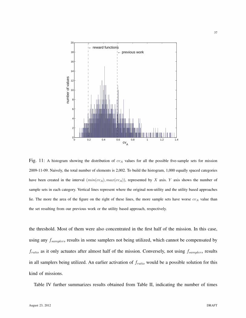
0 0.2 0.4 0.6 0.8 1 1.2 1.40

2

4

6

8

10

12

14

16

18

20

← previous work← reward functions

num

ber

of v

alue

s

cvA

Fig. 11: A histogram showing the distribution of cvA values for all the possible five-sample sets for mission

2009-11-09. Naively, the total number of elements is 2,002. To build the histogram, 1,000 equally spaced categories

have been created in the interval (min(cvA),max(cvA)), represented by X axis. Y axis shows the number of

sample sets in each category. Vertical lines represent where the original non-utility and the utility based approaches

lie. The more the area of the figure on the right of these lines, the more sample sets have worse cvA value than

the set resulting from our previous work or the utility based approach, respectively.

the threshold. Most of them were also concentrated in the first half of the mission. In this case,

using any fsamplers results in some samplers not being utilized, which cannot be compensated by

fratio as it only actuates after almost half of the mission. Conversely, not using fsamplers results

in all samplers being utilized. An earlier activation of fratio would be a possible solution for this

kind of missions.

Table IV further summarizes results obtained from Table II, indicating the number of times


38# of # of Percentile

Mission hot- sample Metric Previous Rewardspots sets Approach Function

2008-05-12 26 65,780cvΣ 13 71cvA 68 68cvµ 25 82

2008-06-26 54 3,162,510cvΣ 42 59cvA 43 43cvµ 26 52

2008-11-10 39 575,757cvΣ 6 7cvA 12 23cvµ 19 19

2009-11-04 6 6cvΣ 0 0cvA 0 0cvµ 0 0

2009-11-09 14 2,002cvΣ 50 68cvA 27 95cvµ 48 81

2009-11-10 13 1,287cvΣ 1 10cvA 1 14cvµ 0 1

2009-11-13 13 1,287cvΣ 75 99cvA 95 99cvµ 41 84

2009-12-08 12 792cvΣ 2 29cvA 5 28cvµ 0 1

2010-03-23 3 1cvΣ – –cvA – –cvµ – –

2010-07-011

1cvΣ – –cvA – –cvµ – –

TABLE III: Previous work [12], [29] and best reward function percentiles for each of the three metrics with

respect to all the possible sample sets. Values for the two last missions are omitted as they have less than 5 hot-spots.

using a given profile results in the best value of the metric. While the data sets are not statistically

expansive, we do have some preliminary lessons learned from these experiments. As the table

shows, #2 gives the best results overall for two of the three metrics; therefore if no Feature

Aware strategies are implemented it should be the default choice. Performance for #4 is quite

close to that of #2, so it is also a good choice. #4 is slightly more restrictive than #2, so it should

be used when there is a strong indication of dispersed hot-spots. In addition, #4, prevents taking

samples unless at least half of the imposed distance constraint is met, so it is especially useful


39fdistance fsamplers

Metric #1 #2 #4 #7 #8 #10 #11 nonecvΣ 4 6 5 1 3 2 3 4cvA 6 5 4 0 2 2 3 7cvµ 5 6 6 0 4 2 2 5

TABLE IV: Summary of Table II indicating the number of times using a utility function profile results in the

best combination also highlighted in bold in that table.

when the field is rich and hot-spots are quite close to one another. #1 performs better than #2

when spatial coverage (cvA) is a factor, but for the remainder two metrics their use does not

yield appreciably better results. Therefore #1 is relevant when spatial coverage is to be factored.

In the case of sampler functions, not using any appears appropriate. This is specially true in

missions with low feature signal or with high triggering threshold. In feature rich situations, #8

performs quite well.

Except for cvµ in 2009-11-13, using fratio gives better or equivalent results for all the metrics

than not using it. In that mission, except for a peak at the beginning, the feature is concentrated

towards the end of the mission. Use of fratio produces a sample to be taken in a small peak in

the middle of the mission, wasting one sampler that could have been more useful towards the

end. Therefore unless the feature is expected to be concentrated at the end and spatial coverage

is not the primary concern, use of fratio is recommended.

In addition to testing our utility based approach on past missions, we ran an at-sea experiment

on July 1st, 2010. A low FOI was expected, so the triggering threshold was set at 0.21. To avoid

exhausting samples early in the mission, the spatial sampling constraint was set for a distance

of 2.5 km and fdist was set to #4, to ensure that at least half of this distance constraint would be

enforced between two samples. Further, to acquire some samples at the beginning of the mission

to counteract the expected weak FOI, fsamplers #10 was chosen. The aim was not to increase


40the threshold until at least half of the samples were taken. At sea, not only was the FOI low

with 99% of the time under a threshold of 0.1, post-mission analysis indicated that the feature

characteristics were unusual and not foreseen by the model in [29], which was used to obtain the

Z ′(v) FOI estimate. Despite this, the utility based approach was able to trigger two samplers, at

the only two hot-spots detected, whereas the nominal non-utility approach would have triggered

only one, while missing the second peak, which was less than 2.5 km away from the first.

B. Triggering Threshold Sensitivity Analysis

One short-coming of our approach is the need to establish a triggering threshold before the

mission. The lower the threshold, the more local maxima will be considered as hot-spots, thereby

increasing possible locations for sampling.

Fig. 12 shows the variations in the number of hot-spots for all the 10 missions when the

threshold is increased by 0.01 steps in the interval [0.01, 0.99]. In all cases, hot-spots found

within a 60 second temporal window are grouped together and considered to represent the same

hot-spot (the AUV ground speed is about 1.36 m/s, the distance is less than 90 meters and

therefore not significant for capturing biological diversity). As the figure shows, number of hot-

spots increases almost exponentially as the threshold is lowered. Even a small reduction on the

triggering threshold increases the number of hot-spots in almost all missions.

From the figure, one can distinguish two types of missions; those where the number of hot-

spots vary smoothly and those which are piecewise linear. If we compare Fig. 12 with tables II

and III, we can see that our approach behaves better in missions where the number of hot-spots

varies without many granular steps. This is also the case for missions where the threshold is not

set high; so not only are several hot-spots found, but a small threshold increase assures a wide

range of locations to sample, leaving the combined work of fsamplers and fratio to provide for


41

0 0.2 0.4 0.6 0.8 10

50

100

150

200

Sampling Threshold

Num

ber

of h

ot−

spot

s de

tect

ed

(a) 2008-05-12

0 0.2 0.4 0.6 0.8 10

50

100

150

200

Sampling Threshold

Num

ber

of h

ot−

spot

s de

tect

ed

(b) 2008-06-26

0 0.2 0.4 0.6 0.8 10

50

100

150

200

Sampling Threshold

Num

ber

of h

ot−

spot

s de

tect

ed

(c) 2008-11-10

0 0.2 0.4 0.6 0.8 10

50

100

150

200

Sampling Threshold

Num

ber

of h

ot−

spot

s de

tect

ed

(d) 2009-11-04

0 0.2 0.4 0.6 0.8 10

50

100

150

200

Sampling Threshold

Num

ber

of h

ot−

spot

s de

tect

ed

(e) 2009-11-09

0 0.2 0.4 0.6 0.8 10

20

40

60

80

100

Sampling Threshold

Num

ber

of h

ot−

spot

s de

tect

ed

(f) 2009-11-10

0 0.2 0.4 0.6 0.8 10

50

100

150

200

Sampling Threshold

Num

ber

of h

ot−

spot

s de

tect

ed

(g) 2009-11-13

0 0.2 0.4 0.6 0.8 10

20

40

60

80

100

Sampling Threshold

Num

ber

of h

ot−

spot

s de

tect

ed

(h) 2009-12-08

0 0.2 0.4 0.6 0.8 10

50

100

150

200

Sampling Threshold

Num

ber

of h

ot−

spot

s de

tect

ed

(i) 2010-03-23

0 0.2 0.4 0.6 0.8 10

0.5

1

1.5

2

2.5

3

3.5

4

Sampling Threshold

Num

ber

of h

ot−

spot

s de

tect

ed

(j) 2010-07-01

Fig. 12: Variation of the number of found hot-spots with respect to the sampling threshold Tf , for the 10 missions.The vertical line represents the actual threshold chosen for each mission.

desired spatial coverage.

To evaluate the robustness of our approach we have repeated the calculations shown in Table

III for 10 different thresholds, resulting from altering the original threshold in steps of 5% in


42the interval [-25%,25%]. Reductions over 25% are known to generate hot-spots with a very low

value of yv. In reality, for 7 out of the 10 missions a 10% increase yields no hot-spots. As an

example, Fig. 13 shows the variations of percentiles for the three metrics for mission 2009-11-

09. cvµ percentiles are the most stable, with little dependence on the threshold. Conversely, the

values for cvA change substantially as the threshold is reduced. There are two reasons for this;

for low thresholds the poor spatial coverage is due to an early utilization of samplers, which

cannot be compensated by fsamplers. A more steep profile, as in #9, would probably improve the

performance. For thresholds closer to the original, most hot-spots discovered have values only

slightly higher than the threshold. As noted previously for 2008-11-10, not using fsamplers quickly

uses up the samplers, while using it results in empty samplers returned. An earlier activation of

fratio, for example automatically driven by the values of the hot-spots found, would solve the

problem.

VIII. CONCLUSION

We present a utility based technique for discrete adaptive sampling. The principal aim is to

integrate available information including science and operational constraints to decide where a

set of samples can be taken. To do so, a utility is computed based on a priori knowledge and

presumed scientific intent; our current work deals with Weakly Informed and Mission Aware

strategies with the expectation of inclusion of feature aware strategies in the future using the

existing framework. The utility based approach is especially useful in sequential sampling; new

information obtained with previous samples can be integrated to acquire further samples. We

show how the approach compares against a previously published technique using historical AUV

data. The target application is in sampling Intermediate Nepheloid Layers (INL); however the

techniques are general and can be applied to sample most oceanic scalar fields when no a priori


43

−25 −20 −15 −10 −5 010

20

30

40

50

60

70

80

90

100

Percentage of threshold variation

Per

cent

ile

cvΣcv

Acvµ

Fig. 13: Variation of the reward function percentiles for the three metrics when the threshold is reduced down by25% in steps of 5%, for November 9th, 2009 mission. No hot-spots are found when the threshold is increased. Xaxis represents the threshold changes in percentage. Y axis shows the percentiles. Values for x = 0 are those oftable III.

model of the feature is available.

We also provide guidance on the appropriate choice of optimization metrics depending on sci-

entific preference for spatial coverage, hot-spot capture or a mix between the two. Experimental

results have shown that, even with Weakly Informed utility functions, our approach performs

better using all the three metrics in comparison to the approach suggested in [29].

This initial effort in sampling has been promising and is likely to lead our work in a number

of different directions. First, we plan to investigate the synthesis of utility functions applying

Machine Learning techniques to historical data; using clustering techniques for mission clas-

sification as a means to learn suitable utilities as reward functions is one approach. The idea

behind this is to explore whether there are ’typical’ mission types: with the FOI concentrated


44at the beginning/end, patchy, with many/few hot-spots, etc. The scientist could have a general

idea of what kind of feature distribution to expect, so the parameterization of functions could

be automated. This will require more historical data than what is currently available, both for

clustering and for the automatic selection of parameters for each cluster.

The long term goal is to experiment with Feature Aware strategies where some a priori

knowledge of the field is available. We plan to build a probabilistic model of the feature of

interest as the AUV makes in situ measurements. One approach is by using Gaussian Process

Regression [18] or Kriging as used in spatial statistics. This allows us to estimate the signal and

its uncertainty at unobserved points, and the utility can be altered depending on their proximity

to high-value sample points. Such a model could also be used to predict peaks of the feature of

interest [8]. Given the temporal variability of oceanic features even in very short time periods,

the accuracy of such models for oceanographic phenomena needs study, especially for those

learned offline. Also, using such models, de-correlation scales of features of interest from past

data can be learned. From the models we can obtain a kernel function or variogram that defines

the spatial variability of the data. This can directly be used as an utility function.

A model of the field can also potentially be available using synthetic ocean models such

as [46]; however the inclusion of dynamic features to be modeled within such systems is still

tentative since there is poor to little understanding of such coastal features. Limited skill at the

meso-scale in of itself poses a substantial challenge in the use of such techniques.

A more empirical approach to incorporate feature awareness is to potentially observe the

survey area rapidly with the AUV and in the process build an approximate “map” of the field.

This allows in situ inference to determine the overall characteristics of the survey area and have

the vehicle revisit the vicinity of those locations that have FOI peaks. Having a map of the feature

of interest will allow planning ahead for possible observations with better information. However,


45this approach is strongly dependent on the rates of feature evolution and the survey volume. In

a large survey, returning back to location(s) of potential interest which may be impacted by

tides, might not be scientifically interesting. Surveys could also be augmented with shore-side

support from a skilled oceanographer guiding the AUV with targeted commands with support

from remote-sensing data or other synoptic views of the coastal ocean. Our efforts to date are

focused more on the latter as a means to augment on-board situational awareness on the AUV

[9]. Finally, having an a priori estimation of a FOI by any of the former techniques will also

allow in situ estimation of the quality metrics to be included in utility calculations.

IX. ACKNOWLEDGMENT

We thank our colleagues Thom Maughan, Tom O’Reilly, John Ryan, Julio Harvey, Hans

Thomas, Bob Vrijenhoek and the crew of the R/V Zephyr for their valuable support. We thank

Timothy Chung of NPS and Rishi Graham of MBARI for their valuable comments on an early

draft of this paper. Finally, we wish to thank the three anonymous reviewers for their helpful

suggestions in revising the manuscript.

REFERENCES

[1] AURENHAMMER, F. Voronoi diagrams - a survey of a fundamental geometric data structure. ACM Comput. Surv. 23, 3

(1991), 345–405.

[2] BARTAK, R. Modelling soft constraints: a survey. Neural Network World 12, 5 (2002), 421–431.

[3] BARTH, N., AND WUNSCH, C. Oceanographic experiment design by Simulated Annealing. Journal of Physical

Oceanography 20, 9 (1990), 1249–1263.

[4] BINNEY, J., KRAUSE, A., AND SUKHATME, G. S. Informative path planning for an autonomous underwater vehicle. In

Intnl. Conf. on Robotics & Automation (2010).

[5] BIRD, L., SHERMAN, A., AND RYAN, J. P. Development of an active, large volume, discrete seawater sampler for

autonomous underwater vehicles. In Proc Oceans MTS/IEEE Conference (Vancouver, Canada, 2007).


46[6] BISTARELLI, S., MONTANARI, U., ROSSI, F., SCHIEX, T., VERFAILLIE, G., AND FARGIER, H. Semiring-based csps and

valued csps: Frameworks, properties, and comparison. Constraints 4 (1999), 199–240.

[7] BRODIE, M., RISH, I., AND MA, S. Optimizing probe selection for fault localization. 12th Intnl. Workshop on Distributed

Systems Operation and Maintenance (DSOM) (October 2001).

[8] COX, D., COX, L. H., AND ENSOR, K. B. Spatial sampling and the environment: some issues and directions. Environmental

and Ecological Statistics 4 (1997), 219–233.

[9] DAS, J., MAUGHAN, T., MCCANN, M., GODIN, M., O’REILLY, T., MESSIE, M., BAHR, F., GOMES, K., PY, F.,

BELLINGHAM, J., SUKHATME, G., AND RAJAN, K. Towards mixed-initiative, multi-robot field experiments: Design,

deployment, and lessons learned. In Proc. Intelligent Robots and Systems (IROS) (San Francisco, California, 2011).

[10] DESHPANDE, A., GUESTRIN, C., MADDEN, S., HELLERSTEIN, J., AND HONG, W. Model-driven data acquisition in

sensor networks. In International Conference on Very Large Data Bases (2004), pp. 588–599.

[11] FERRI, G., JAKUBA, M., AND YOERGER, D. A novel method for hydrothermal vents prospecting using an autonomous

underwater robot. In IEEE International Conference on Robotics and Automation (may 2008), pp. 1055–1060.

[12] FOX, M., LONG, D., PY, F., RAJAN, K., AND RYAN, J. P. In situ analysis for intelligent control. In Proc. of IEEE/OES

OCEANS Conference (2007), IEEE.

[13] FROLOV, S., BAPTISTA, A., AND WILKIN, M. Optimizing fixed observational assets in a coastal observatory. Continental

Shelf Research 28, 19 (2008), 2644 – 2658.

[14] HARVEY, J. B. J., AND GOFF, L. J. A reassessment of species boundaries in cystoseira and halidrys (fucales, phaeophyceae)

along the north american west coast. Journal of Phycology 42 (2006), 707–720.

[15] INCZE, M. L. Optimized deployment of autonomous underwater vehicles for characterization of coastal waters. Journal

of Marine Systems 78, Supplement 1 (2009), S415 – S424. Coastal Processes: Challenges for Monitoring and Prediction.

[16] JONES, W. J., PRESTON, C. M., III, R. M., SCHOLIN, C. A., AND VRIJENHOEK, R. C. A robotic molecular method for

in situ detection of marine invertebrate larvae. Molecular Ecology Resources 8 (2008), 540–550.

[17] K., G. S., JONES, W. J., SCHOLIN, C. A., MARIN, R., AND VRIJENHOEK, R. C. Molecular detection of marine

invertebrate larvae. Marine Biotechnology 8 (2006), 149–160.

[18] KRAUSE, A., AND GUESTRIN, C. Nonmyopic active learning of Gaussian Processes: an exploration-exploitation approach.

In Intnl. Conf. on Machine Learning (New York, NY, USA, 2007), ACM, pp. 449–456.

[19] KRAUSE, A., LESKOVEC, J., GUESTRIN, C., VANBRIESEN, J., AND FALOUTSOS, C. Efficient sensor placement

optimization for securing large water distribution networks. Journal of Water Resources Planning and Management 134,

6 (2008), 516–526.

[20] KRAUSE, A., SINGH, A., AND GUESTRIN, C. Near-Optimal sensor placements in Gaussian Processes: Theory, efficient


47algorithms and empirical studies. J. Mach. Learn. Res. 9 (2008), 235–284.

[21] KUMAR, S., CELORRIO, S., PY, F., KHEMANI, D., AND RAJAN, K. Optimizing Hidden Markov Models for Ocean Feature

Detection. In Proceedings 24th Intnl. Florida AI Research Society (FLAIRS) (Palm Beach, FL, 2011), pp. 39–44.

[22] LEGENDRE, P., DALE, M., FORTIN, M., GUREVITCH, J., AND HOHN, M. The consequences of spatial structure for the

design and analysis of ecological field surveys. Ecography 25 (2002), 601–615.

[23] LEONARD, N., PALEY, D., LEKIEN, F., SEPULCHRE, R., FRATANTONI, D., AND DAVIS, R. Collective motion, sensor

networks, and ocean sampling. Proceedings of the IEEE 95, 1 (January 2007), 48–74.

[24] LEONARD, N. E., PALEY, D. A., DAVIS, R. E., FRATANTONI, D. M., LEKIEN, F., AND ZHANG, F. Coordinated control

of an underwater glider fleet in an adaptive ocean sampling field experiment in monterey bay. Journal of Field Robotics

27, 6 (2010), 718–740.

[25] LONG, E., AND WILSON, C. On the identification of toxic hot spots using measures of sediment quality triad. Marine

Pollution Bulletin 34 (1997), 373–374.

[26] LOW, K. H. Multi-Robot Adaptive Exploration and Mapping for Environmental Sensing Applications. PhD thesis, Carnegie

Institute of Technology, Carnegie Melon University, 2009.

[27] MARINONE, S. G., ULLOA, M. J., PARES-SIERRA, A., LAVIN, M. F., AND CUDNEY-BUENO, R. Connectivity in the

northern gulf of california from particle tracking in a three-dimensional numerical model. Journal of Marine Systems 71

(2008), 149–158.

[28] MATHERON, G. Principles of geostatistics. Economic Geology 58 (1963), 1246–1266.

[29] MCGANN, C., PY, F., RAJAN, K., RYAN, J., THOMAS, H., HENTHORN, R., AND MCEWEN, R. Preliminary results for

model-based adaptive control of an autonomous underwater vehicle. In Experimental Robotics, O. Khatib, V. Kumar, and

G. Pappas, Eds., vol. 54 of Springer Tracts in Advanced Robotics. Springer Berlin / Heidelberg, 2009, pp. 395–405.

[30] MCGANN, C., PY, F., RAJAN, K., RYAN, J. P., AND HENTHORN, R. Adaptive control for autonomous underwater vehicles.

In Assoc. for the Advancement of Artificial Intelligence (AAAI) (Chicago, IL, 2008), vol. 3, pp. 1319–1324.

[31] MCGANN, C., PY, F., RAJAN, K., THOMAS, H., HENTHORN, R., AND MCEWEN, R. A Deliberative Architecture for

AUV Control. In Intnl. Conf. on Robotics and Automation (ICRA) (Pasadena, May 2008).

[32] MCPHEE-SHAW, E. Boundary-interior exchange. reviewing the idea that internal-wave mixing enhances lateral dispersal

near continental margins. Deep-Sea Research II 53 (Jan 2006), 45–49.

[33] OLIVEIRA, V. D., AND ECKER, M. D. Bayesian hot spot detection in the presence of a spatial trend: application to total

nitrogen concentration in Chesapeake Bay. Environmetrics 13 (2002), 85–101.

[34] OZMUTLU, H., GAUTAM, N., AND BARTON, R. Managing end-to-end network performance via optimized monitoring

strategies. Journal of Network and Systems Management 10 (2002).


48[35] POPA, D., SANDERSON, A., HOMBAL, V., KOMERSKA, R., MUPPARAPU, S., BLIDBERG, R., AND CHAPPEL, S. Optimal

sampling using singular value decomposition of the parameter variance space. In Intelligent Robots and Systems, 2005.

(IROS 2005). 2005 IEEE/RSJ International Conference on (August 2005), pp. 3131 – 3136.

[36] PY, F., RAJAN, K., AND MCGANN, C. A Systematic agent framework for situated autonomous systems. In 9th

International Conf. on Autonomous Agents and Multiagent Systems (Toronto, Canada, May 2010), International Foundation

for Autonomous Agents and Multiagent Systems, pp. 583–590.

[37] RAHIMI, M., PON, R., KAISER, W. J., SUKHATME, G. S., ESTRIN, D., AND SRIVASTAVA, M. Adaptive sampling for

environmental robotics. In IEEE International Conference on Robotics and Automation (2003), pp. 3537–3544.

[38] RASMUSSEN, C. E., AND WILLIAMS, C. Gaussian processes for machine learning. MIT Press, Cambridge, 2006.

[39] RIGBY, P., PIZARRO, O., AND WILLIAMS, S. B. Toward adaptive benthic habitat mapping using gaussian process

classification. Journal of Field Robotics (2010), 741–758.

[40] RIGBY, P., WILLIAMS, S. B., PIZARRO, O., AND COLQUHOUN, J. Effective benthic surveying with autonomous

underwater vehicles. In MTS/IEEE Oceans (Vancouver, Canada, september 2007).

[41] RUDNICK, D., AND PERRY, M. ALPS: Autonomous and Lagrangian Platforms and Sensors, Workshop Report. Tech. rep.,

www.geo-prose.com/ALPS, 2003.

[42] RYAN, J., YODER, J., AND TOWNSEND, D. Influence of a gulf stream warm-core ring on water mass and chlorophyll

distributions along the southern flank of georges bank. Deep-Sea Research II 48 (2001), 159–178.

[43] RYAN, J. P., CHAVEZ, F. P., AND BELLINGHAM, J. G. Physical-biological coupling in monterey bay, california:

Topographic influences on phytoplankton ecology. Marine Ecology Progress Series 287 (2005), 23–32.

[44] RYAN, J. P., JOHNSON, S., SHERMAN, A., RAJAN, K., PY, F., THOMAS, H., HARVEY, J., BIRD, L., PADUAN, J.,

AND VRIJENHOEK, R. Mobile autonomous process sampling within coastal ocean observing systems. Limnology &

Oceanograhy: Methods 8 (2010), 394–402.

[45] SCHOLIN, C. A., MARIN, R., MILLER, P. E., DOUCETTE, G., POWELL, C., HOWARD, J., HAYDOCK, P., AND RAY, J.

Application of dna probes and a receptor binding assay for detection of pseudo-nitzschia (bacillariophyceae) species and

domoic acid activity in cultured and natural samples. Journal of Phycology 35 (1999), 1356–1367.

[46] SHCHEPETKIN, A. F., AND MCWILLIAMS, J. C. The regional oceanic modeling system (ROMS): a split-

explicit, free-surface, topography-following-coordinate oceanic model. Ocean Modeling 9 (2005), 347–404.

doi:10.1016/j.ocemod.2004.08.002.

[47] SINGH, A., BATALIN, M., STEALEY, M., CHEN, V., HANSEN, M., HARMON, T., SUKHATME, G., AND KAISER, W.

Mobile robot sensing for environmental applications. In Field and Service Robotics, C. Laugier and R. Siegwart, Eds.,

vol. 42 of Springer Tracts in Advanced Robotics. Springer Berlin / Heidelberg, 2008, pp. 125–135.


49[48] SUN, F., XU, W., JIN, L., AND LI, J. Path planning of autonomous underwater vehicles for optimal environmental

sampling. In OCEANS 2010 IEEE - Sydney (may 2010), pp. 1–4.

[49] VIV-TRUYOLS, G., TORRES-LAPASI, J., VAN NEDERKASSEL, A., HEYDEN, Y. V., AND MASSART, D. Automatic

program for peak detection and deconvolution of multi-overlapped chromatographic signals: Part i: Peak detection. Journal

of Chromatography A 1096, 1-2 (2005), 133 – 145. Chemical Separations and Chemometrics.

[50] WILLCOX, J. S., BELLINGHAM, J. G., ZHANG, Y., AND BAGGEROER, A. B. Performance metrics for oceanographic

surveys with autonomous underwater vehicles. IEEE J. Oceanic Engineering 26 (2001), 711–725.

[51] YOERGER, D. R., JAKUBA, M., BRADLEY, A. M., AND BINGHAM, B. Techniques for deep sea near bottom survey using

an autonomous underwater vehicle. The International Journal of Robotics Research 26, 1 (January 2007), 41–54.

[52] ZHANG, B. Adaptive Sampling with a Robotic Sensor Network. PhD thesis, University of Southern California, 2008.

[53] ZHANG, Y., AND BELLINGHAM, J. G. An efficient method of selecting ocean observing locations for capturing the leading

modes and reconstructing the full field. Journal of Geophysical Research 113 (2008).

[54] ZHANG, Y., MCEWEN, R., RYAN, J., AND BELLINGHAM, J. Design and tests of an adaptive triggering method for

capturing peak samples in a thin phytoplankton layer by an autonomous underwater vehicle. IEEE Journal of Oceanic

Engineering 35, 4 (Oct 2010), 785–796.

[55] ZHU, Z., AND STEIN, M. Spatial sampling design for prediction with estimated parameters. Journal of Agricultural,

Biological, and Environmental Statistics 11, 1 (March 2006), 24–44.


sampling dynamic ocean fields - uc3magolaya/download/papers/joe-12.pdf · sampling dynamic ocean...

Documents