sample size determination for step-down multiple test procedures

Journal of Statistical Planning and Inference 27 (1991) 271-290

North-Holland

271

Sample size determination for step-down multiple test procedures: Orthogonal contrasts and comparisons with a control

Anthony J. Hayter

Department of Mathematics, University of Bath, Bath BA2 7A Y, U.K.

Ajit C. Tamhane

Department of Statistics, Northwestern University, Evanston, IL 60208, U.S.A.

Received 1 June 1989; revised manuscript received 18 January 1990

Recommended by S. Panchapakesan

Abstrucr; We address the problem of sample size determination for step-down multiple comparison

procedures (MCP’s) for two nonhierarchical families - orthogonal contrasts and comparisons with a

control, in order to guarantee a specified requirement on their power. The results for the corresponding

single-step MCP’s are obtained as special cases.

Numerical calculations of the sample sizes to guarantee a specified power requirement are carried out

for the one-sided comparisons with a control problem in selected cases. These calculations show that for

the cases considered, about 10% to 20% savings can be achieved in the total sample size by using the

step-down MCP of Miller (1966, pp. 85-86) instead of the single-step MCP of Dunnett (1955). The

percentage savings increase, as expected, with the number of treatments being compared with the control.

In the process of determining the smallest total sample size for each MCP to guarantee the specified

power requirement, we also determine the optimum allocation of this sample size among the treatments

and the control. We find that the square root allocation rule recommended by Dunnett (1955) provides

a reasonable approximation to the optimum allocation for both the MCP’s.

AMS Subject Classification: Primary 62515; secondary 62K99.

Key words and phrases: Multiple comparisons; single-step procedures; step-down procedures; power;

sample size determination; orthogonal contrasts; comparisons with a control; multivariate t-distribution;

normal distribution.

1. Introduction

It is well-known that step-down multiple comparison procedures (MCP’s) are

more powerful than their single-step counterparts for simultaneous testing prob-

0378-3758/91/$03.50 0 1991-Elsevier Science Publishers B.V. (North-Holland)

212 A. J. Hayter, A.C. Tamhane / Sample size for multiple test procedures

lems. (For the terminology used in this article we refer the reader to Hochberg and

Tamhane (1987).) Although step-down MCP’s have been used for this reason for

a long time, the important design problem of sample size determination to guarantee

a specified power requirement has not been yet addressed for these procedures. The

sample size determination problem for single-step MCP’s is considered in Chapter

6 of Hochberg and Tamhane (1987) and more recently in Hsu (1988).

In the present article we solve the sample size determination problem for step-

down and single-step MCP’s for the families of orthogonal contrasts and com-

parisons with a control under the normality setup. This enables us to make a quan-

titative assessment of the savings in the total sample size achieved by step-down

MCP’s relative to their single-step counterparts. We have carried out these com-

putations for the family of one-sided comparisons with a control, where Dunnett’s

(1955) single-step MCP is compared with the step-down MCP originally proposed

by Miller (1966, pp. 85-86). The same step-down MCP was independently proposed

by Naik (1975) and was shown to satisfy the type I familywise error rate requirement

by Marcus, Peritz and Gabriel (1976).

The following is the outline of the present article: Section 2 gives the

preliminaries. These include the distributional setup assumed, the hypotheses and

the associated probability requirements (type I familywise error rate and power),

and the descriptions of the single-step and step-down MCP’s under consideration.

Two families of multiple comparisons of particular interest to us, namely, the

families of orthogonal contrasts and comparisons with a control are also described.

Section 3 states the principal theoretical results concerning the least favorable con-

figurations of the MCP’s; the proofs of these results are postponed to the Appendix.

Section 4 applies these results to the problem of one-sided comparisons with a con-

trol, and gives tables of the ‘optimal’ sample sizes that must be taken on each one

of the treatments and the control to guarantee the specified power requirement.

These sample sizes are tabulated both for the single-step MCP of Dunnett (1955)

and the step-down MCP of Miller (1966), and they are used to make assessments

of the relative savings achieved by the latter MCP. Finally some concluding remarks

are given in Section 5.

2. Preliminaries

2. I. Distributional setup

Consider the standard linear model setting and let e= (8,, . . . , ok) be the best

linear unbiased estimator of the unknown parameter vector of interest 0=

(0 I, . . . , 0,). We assume that the gj are jointly normally distributed with means Bi,

a common variance 02u and a common correlation Q= corr(8,, 4). (1 si#j<k)

where v>O and 05~ < 1 are known constants and 02>0 is an unknown scalar. We

further assume that an unbiased estimator S* of o2 is available based on v degrees

A. J. Hayter, A. C. Tamhane / Sample size for multiple test procedures 273

of freedom (d.f.) which is distributed independently of 0 as a a2xz/v random

variable (T.v.). Two examples of this distributional setup which are of particular in-

terest to us are given in Section 2.4.

2.2. Hypotheses and probability requirements

We consider the following two families of hypotheses testing problems:

(I) One-sided: Hb’,‘: BilO VS. Hi:‘: B;>O (1 5il:k). (2.1)

(II) Two-sided: H$‘: 8,=0 vs. Hi;‘: 8;#0 (1 lirk). (2.2)

In the case of (2.2), it is often desired to make a directional decision (i.e., decide

that Bj> 0 or < 0) for any Hg) that is rejected (1 I is k). For each testing problem we want the MCP that we use to satisfy the following

type I familywise error rate (FWE) requirement:

PO{any true H$) is rejected (1 Siz%k)] S(Y for all 8 (j= 1,2), (2.3)

where 0 < o < 1 is specified. In addition, for design purposes we postulate the follow-

ing power requirements for (2.1) and (2.2); in these requirements 6>0 and

0 < p < 1-o are specified constants.

(I) One-sided tests :

P,{all false Hi\’ with Oj>& are rejected} 2 1 -p for all 8.

(IIa) Two-sided tests (without directional decisions):

P,(all false HgJ with 119; 1 Z&T are rejected} 2 1-p for all 8.

(IIb) Two-sided tests (with directional decisions):

Ps { all false HE) with 18; 1 2 60 are rejected with correct

directional decisions} L 1 -p for all 8.

2.3. Procedures

(2.4)

(2.5)

(2.6)

The common step-down and single-step MCP’s (which can be shown to have cer-

tain optimality properties) for the testing problems (2.1) and (2.2) are based on the

test statistics

(2.7)

Under the configuration 8, = ... =e,=O (lsmlk), the r.v.‘s T,,T, ,..., T, have a

joint m-variate central t-distribution with v d.f. and common associated correlation

e (see Hochberg and Tamhane (1987, Appendix 3) for a definition of this distribu-

tion); for m = 1, this of course reduces to the univariate Student’s t-distribution. We

denote the upper (r point of maxlcjcm T by tg,)v,e (for m = 1 simply by t$@) and

214 A.J. Hayter, A.C. Tamhane / Sample size for multiple test procedures

that of maxl,ism ITi\ by IfI~!Y,e t(a)

(which equals tf’2) for m = 1). The critical points

m,v,e and lfl%.e have been tabulated by Bechhofer and Dunnett (1988) for

selected values of a, m, v and Q.

The single-step MCP for the one-sided testing problem (2.1) rejects any Hrj in

favor of H’*.’ if 11

T> fg’,,,@ (1 sisk). (2.8)

We shall refer to this MCP as SSl. Similarly the single-step MCP for the two-sided

testing problem (2.2) rejects any HE’ in favor of Hz’ if

[7;[> it\ge (lsirk). (2.9)

Rejection of any HE’ can be accompanied by a directional decision that Bi>O if

q>O and 0i<O if T,<O (lsisk). We shall refer to this MCP as SS2.

It can be shown that both SSl and SS2 satisfy the FWE requirement (2.3) (see

Hochberg and Tamhane (1987, Ch. 3, Sec. 2)).

The step-down MCP for the one-sided testing problem (2.1) begins by ordering

the statistics (2.7) as T(i)5 Tc2)z? ... 5 Ttk,. Let Hb’(‘,,, H$,, . . . . H& be the corre-

sponding hypotheses. At step 1, H$, is tested by comparing T,,, with tg),,@. If

T(k, 5 $:., then all Hi) are retained (i.e., not rejected) without further tests.

If Tck)> tj& then H& is rejected and Ht)k_,, is tested next by comparing Tck_Ij with tp!,,,,,. In general, H&, is tested and rejected iff T(,)> $,$ for

l=k,k- l,...,m; if H,(,) (I) is tested and not rejected because T(,)s tz,)v,Q then the (1) hypotheses H$,, . . . , He,, _ i) are retained without actually testing them. We shall

refer to this MCP as SDl.

The step-down MCP for the two-sided testing problem (2.2) operates exactly in

the same manner as above except now the ordered absolute values of the statistics

(2.7), viz., ITI& /77~2,5--5 ITi( are used and the critical constants tg!,,e are

replaced by 1 t ( g!v,e (15 m 5 k). Rejection of any Hgj can be accompanied by a

directional decision in the usual manner. We shall refer to this MCP as SD2.

It can be shown that both SD1 and SD2 satisfy the FWE requirement (2.3) (see

Hochberg and Tamhane (1987), Ch. 3, Sec. 4.2)). Also note that since tt),,,,> t$,,, and similarly 1t\tt,,> Itl$!v,e for m= 1, . . . . k- 1 and for any a, v and Q, the step-

down MCP’s SD1 and SD2 are more powerful than the respective single-step MCP’s

SSl and SS2.

Remark 1. If type III errors associated with directional decisions are included in the

definition of the FWE then it is not known whether or not SD2 satisfies (2.3) in all

cases (see, e.g., Shaffer (1980)) although SS2 clearly does so (see Hochberg and

Tamhane (1987, Ch. 2, Sec. 2.3.2)). However, type III errors are considered as part

of the power requirement (2.6) and not as part of the FWE requirement in the pre-

sent formulation. This seems to us a more natural way of treating type III errors.


2.4. Examples

Example 1 (Orthogonal contrasts). Consider a completely randomized experiment

with pz2 factorial treatment combinations having cell means pj (1 ~jlp), a com-

mon error variance a* and n 2 2 replications per cell. Let

where the coefficients Cij satisfy

jcr cg = 0, jgr ci = 1 and i CijCI,j = 0 (1 <i + i/Sk). j=l

Thus the Bi are normalized orthogonal contrasts. Let

Si= i CijXj (Isilk) j=l

where the Xj are the cell sample means, and let S2 be the usual analysis of variance

(ANOVA) mean square error. Then the 6; are independent normal (i.e., the com-

mon correlation e=O) with means Bi and a common variance a2/n, and S2 is

distributed as a2xz/v independent of the e;‘s with v=p(n- 1) d.f.

The critical points fg,)v,o and iflE,),,e needed to apply the MCP’s of the previous

section in this case are referred to as Studentized maximum and Studentized max-

imum modulus critical points, respectively. These critical points are also tabulated

in Bechhofer and Dunnett (1988).

Example 2 (Comparisons with a control). Suppose that there are kr2 treatment

groups labelled 1,2, . . . , k which are to be compared with a control group labelled

0. The observations from the i-th group are assumed to be independent and iden-

tically distributed (i.i.d.) N(pi, a2) r.v.‘s where the ,u; are unknown group means

and o2 is a common unknown error variance. A random sample of size n is drawn

from each one of the treatment groups and another random sample of size no from

the control group.

The parameters of interest are 19; =,u; - ,uo whose best linear unbiased estimators

are Qi=Xj-Xo (1 silk) where & is the sample mean for the i-th group (O~ilk). Here the S;. are correlated normals with means dj =p, -po, a common variance

02(1/n + l/n,) and a common correlation ,Q = n/(n + no). The ANOVA mean

square error s2 is distributed as 02xt/v with v = N- (k + 1) d.f. where N = no + kn is the total sample size.

3. Least favorable configuration results

Our next task is to determine for each MCP described in Section 2.3 the LFC of


the 19,‘s at which the power (as defined by the 1.h.s. of (2.4) for the one-sided

testing problem and the 1.h.s. of (2.5) or (2.6) for the two-sided testing problem)

of that MCP is minimized. For the given design one can then find the smallest total

sample size N, which makes this minimum greater than or equal to the specified

lower bound 1 -P, thus guaranteeing the appropriate power requirement.

Note that for given k and specified (Y and 6, the minimum power at the LFC is

a function of u, Q and v, which in turn are functions of N depending on the design

employed. By varying some of the design parameters it is sometimes possible to

maximize this minimum for given N. This evaluation of the max-min power enables

us to obtain the smallest N to guarantee a specified power requirement. For exam-

ple, in the comparisons with a control problem described in Example 2, if we let

r=nO/n and N=n,+kn then ~={(r+k)(r+l)/rN}“~, ~=l/(l+r) and

v = N- (k + 1). Thus v and Q depend on the design parameter r, which can be chosen

to maximize the minimum power for given N. We shall do this in the computation

of the tables of N for this problem in Section 4.

We now state the result for the one-sided testing problem (2.1). Proofs of all the

results are given in the Appendix.

Theorem 1. For the step-down MCP SDl, the minimum over 8 of

P,{reject Ht/, . . . , H~,~,jO;z6a (lsism), 0,<6a (m+lsi<k)} (3.1)

for fixed m (1 s m i k) is attained when 0; = 60 for 1s is m and 0; = - 03 for m + 1 5 is k. Denoting this minimum by P,,,(SDl), the overall minimum of the 1.h.s. of (2.4) for SD1 is given by min,cm5k P,,(SDl).

Corollary 1. Theorem 1 also holds for the single-step MCP SSl. Moreover, if P,(SSl) denotes the associated minimum value of (3.1) (1 srnc k) then min15m.k Pm(SS1)=Pk(SS1), i.e., for SSl the overall minimum of the 1.h.s. of (2.4) is attained when 9; = 60 for i = 1, . . . , k.

We next state the result for the two-sided testing problem (2.2).

Theorem 2. If Q = 0 then for the step-down MCP SD2, the minimum over 0 of

Pe { reject Hb2,) ,...,HfA) /BJZ6O (llilm), IB;/<Jo (m+l<isk)}

(3.2)

for fixed m (llmsk) is attained when /t9I=&s for l<i<rn and lBi/=O for m + 1 <is k. Denoting this minimum by P,,,(SD2), the overall minimum of the

. 1.h.s. of (2.5) IS given by mmlcmsk P,,,(SD2).

Corollary 2. Theorem 2 also holds for the single-step MCP SS2. Moreover, if P,(SS2) denotes the associated minimum value of (3.2) then mint 5m5k P,,,(SS2) =

A. J. Hayter, A.C. Tamhane / Sample size for multiple test procedures 217

P,(SS2), i.e., for SS2 the overall minimum of the I.h.s. of (2.5) is attained when /Oil =& for i=l,...,k.

Corollary 3. Theorem 2 and Corollary 2 also hold if (3.2) is replaced with

Ps (reject Hi;‘, . . . , HEi, with correct directional decisions )

jO,l2&7 (llilm), /8;l <da (m+ 1 lisk)}. (3.3)

Denoting by P,,,(SD2) and P,(SS2) the associated minimum values of (3.3) we obtain that for SD2 the overall minimum of the t.h.s. of (2.6) is given by mm,cm5k P,(SD2) while that for SS2 is given by mint,,,,, P,(SS2)= P,(SS2),

i.e., for SS2 the overah minimum of the 1.h.s. of (2.6) is attained when JtI,) = 60 .for i= 1, . . . . k.

Remark 2. Theorem 2 does not hold when e>O. In this case the LFC is not simple

and must be numerically determined. It is worth noting, however, that there are ex-

amples where two-sided multiple tests on independent estimates are of interest. One

such example is provided by multiple regression model building where the model is

parametrized so that the effects are orthogonal, e.g., in orthogonal polynomial

regression. Here often no directional decisions are required.

4. Tables of sample sizes for one-sided comparisons with a control

In this section we determine the smallest N= n, + kn and the associated optimal

allocation of the sample sizes, (n,,n), required by SD1 and SSl for guaranteeing

the power requirement (2.4) for selected values of k, a, 6 and 1 -p. Toward this

end we first derive expressions for P,(SDl) (1 <rn<k) and P,(SSl).

4.1. Expressions for minimum powers P,,,

For convenience of notation henceforth we shall use ci to denote t~~~,e (15 is k); here v=N- (k+ 1) and ~=n/(n+n,). To evaluate P,,(SDl) we can take p,=O,

~,=6o (1 (isrn) and p,= -w (m+ 1 <is k). In that case we can represent the

statistics 7; as

T, = zjI/l’e+s~m-zo~ (1 &<m)

I u (4.1)

and T,, , = ..’ = T, = --03 with probability 1. Here the Z, are i.i.d. N(0, 1) r.v.‘s in-

dependent of U, which is distributed as a (x:/v)“* r.v. Using the notation (in-

troduced in the Appendix) (xi, . . . , xp) >*( y,, . . . , y,) to mean x(;, > yy) for i = 1, . . . , p, where the .a+;, and y(,, are the ordered xi’s and y;‘s, respectively, we can write

P,(SDl) = P{(T,, . . ..T.)>*(c,_,+i, . . ..c.)}


=P{(Z,,...,Z,)>*(D,_,+,,...,Dk)} where

Dj = c;U+Z&-6~qiq (k-m+ 1 <is/k).

(4.2)

By conditioning on U = u and Z, = z. and thus on D; = di = ci u + zofi - Sic?, we can write (4.2) as

ICC ‘ca

i ! pcv,, a.., Z,)>*(cLm+,, . . . . 4)1@ (zo)fJ4 dzo du (4.3)

..o I-00

where @(. ) is the standard normal density function and f,( .) is the density func-

tion of a (x;/v)1’2 r.v.

We still need a computable expression for the probability term in the integrand

of (4.3). This is obtained in a recursive form in the following lemma.

Lemma. Form=l,P{Z,>d,}=l-@(dk)andform>l,

P{(Z,, 1.. 9 T,d>*(d,-,+,~...~dd~

= {~(dk~m+2)-~(dk-m+l))P{(Z,,...,Z,~,)>*(dk-,+2,...,dk)}

+ {W-m+j)- @(dkpm+z)IP{(Z1, . . ..Z.p,)

>*(dk-m+,,dk-m+3,...,dk)}

+...+{l-~(d~)}P{(Z,,...,Z,-,)>*(d,-,+,,...,d~~,)} (4.4)

where @(. ) is the standard normal distribution function.

Proof. Condition on Z, to lie in successive intervals: (dk_m+l,dk_,~+21, . . ..(dk. m) which leads to (4.4). Note that we do not condition on Z, to lie in the interval

(-m>dk-,+, ] because in that case HtA cannot be rejected. q

By combining (4.3) with (4.4) a feasible algorithm can be developed to compute

P,(SDl) (1 smsk). Next consider

P,(SSl)= P{T,>ck,...,Tk>ck)

= P(Z,>Dk,...,Zk>Dk}

‘cc ‘Cc =

! i [I- @(&)lk@(zo)f&4 dzo du

<O r-a

where d,+ = cku + zofi - ad-.

(4.5)

Remark 3. For the problem of orthogonal contrasts, we put Q = 0 in (4.3) and (4.5)

and see that they reduce to one-dimensional integrals since the d;= cju - Sfi (15 is k) become free of zo. The expressions for P,(SD2) and pk(SS2) when @ = 0

A.J. Hayter, A.C. Tamhane / Sample size for multiple test procedures 219

can also be readily obtained both when type III errors are ignored (see (3.2)) and

when they are not ignored (see (3.3)).

4.2. Tables

Tables 1, 2 and 3 give the smallest N and the associated optimal allocation (no, n)

required to satisfy the power requirement (2.4) using SD1 and SSl for k=2, 3 and

4, respectively. The calculations are done for o = 0.05, 1 -/I = 0.70, 0.80, 0.90, 0.95,

0.99 and 6=0.5, 1.0. These tables also give the critical constants ci= ti$e required

to implement SD1 and the critical constant ck = tel,, required to implement SSl.

The last column in each table gives the percentage relative saving (RS) in the total

sample size N achieved by SD1 over SSl which is given by

RS = N(SSl) -N(SDl) x 100.

N(SS1)

For given k, a, 6 and (no, n), the power of SD1 under the LFC was computed by

evaluating P,(SDl) (1 smsk) using (4.3) and (4.4) and then taking their

minimum, that for SSl was computed using (4.5). For each given total sample size

N, the maximum of this minimum power over all allocations (nc,n) subject to

N= no+ kn was found for SD1 and SSl. The smallest N for which this max-min

power 2 1 -p and the associated optimal allocation (no, n) were then determined

for these MCP’s. The critical constants ci= t~~~,e (1 I is k) required in this com-

putation were obtained as follows: For i= 1, the corresponding critical point is the

univariate Student’s t critical point, which was obtained using a NAG subroutine.

For i> 1, the desired critical points were obtained by interpolating in the tables of

Bechhofer and Dunnett (1988). As suggested by these authors, interpolation with

Table 1

Optimal sample sizes and critical constants required by SD1 and SSl to guarantee the power requirement

(2.4) (k=2, a=0.05)

6 1-P Step-down procedure SD1 Single-step procedure SSl RS (%)

N n no c2 Cl N n no cz

1 .o 0.70 40 12 16 1.985 1.687 49 15 19 1.972 18.4

0.80 49 15 19 1.972 1.679 59 18 23 1.963 16.9

0.90 64 19 26 1.962 1.670 74 22 30 1.957 13.5

0.95 77 23 31 1.955 1.666 89 27 35 1.950 13.5

0.99 108 32 44 1.947 1.659 120 36 48 1.944 10.0

0.5 0.70 155 47 61 1.939 1.655 187 58 71 1.935 17.1

0.80 191 58 75 1.936 1.653 228 70 88 1.935 16.2

0.90 248 74 100 I.937 1.651 291 88 115 1.936 14.8

0.95 302 89 124 1.938 1.650 350 105 140 1.937 13.7

0.99 426 126 174 1.938 1.648 474 141 192 1.937 10.1

280 A. J. Hayter, A. C. Tamhane / Sample size for multiple test procedures

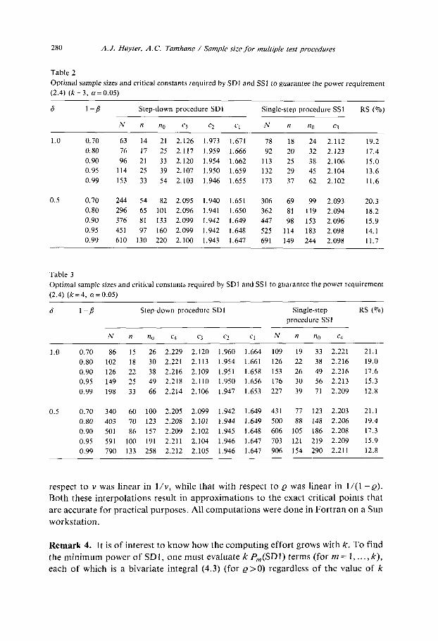
Table 2

Optimal sample sizes and critical constants required by SD1 and SSI to guarantee the power requirement

(2.4) (k=3, cr=O.O5)

6 1-P Step-down procedure SD1 Single-step procedure SSl RS (o/o)

N n n,, c3 c2 Cl N n no c3

1.0 0.70 63 14 21 2.126 1.973 1.671 78 18 24 2.112 19.2

0.80 76 17 25 2.117 1.959 1.666 92 20 32 2.123 17.4

0.90 96 21 33 2.120 1.954 1.662 113 25 38 2.106 15.0

0.95 114 25 39 2.107 1.950 1.659 132 29 45 2.104 13.6

0.99 153 33 54 2.103 1.946 1.655 173 37 62 2.102 11.6

0.5 0.70 244 54 82 2.095 1.940 1.651 306 69 99 2.093 20.3 0.80 296 65 101 2.096 1.941 1.650 362 81 119 2.094 18.2 0.90 376 81 133 2.099 1.942 1.649 447 98 153 2.096 15.9 0.95 451 97 160 2.099 1.942 1.648 525 114 183 2.098 14.1 0.99 610 130 220 2.100 1.943 1.647 691 149 244 2.098 11.7

Table 3

Optimal sample sizes and critical constants required by SD1 and SSl to guarantee the power requirement

(2.4) (k= 4, (Y = 0.05)

6 l-P Step-down procedure SD1 Single-step RS (oio)

procedure SSI

N n no c4 c3 c2 Cl N n no c4

1.0 0.70 86 15 26 2.229 2.120 1.960 1.664 109 19 33 2.221 21.1

0.80 102 18 30 2.221 2.113 1.954 1.661 126 22 38 2.216 19.0

0.90 126 22 38 2.216 2.109 1.951 1.658 153 26 49 2.216 17.6

0.95 149 25 49 2.218 2.110 1.950 1.656 176 30 56 2.213 15.3

0.99 198 33 66 2.214 2.106 1.947 1.653 227 39 71 2.209 12.8

0.5 0.70 340 60 100 2.205 2.099 1.942 1.649 431 77 123 2.203 21.1

0.80 403 70 123 2.208 2.101 1.944 1.649 500 88 148 2.206 19.4

0.90 501 86 157 2.209 2.102 1.945 1.648 606 105 186 2.208 17.3

0.95 591 100 191 2.211 2.104 1.946 1.647 703 121 219 2.209 15.9

0.99 790 133 258 2.212 2.105 1.946 1.647 906 154 290 2.211 12.8

respect to v was linear in I/v, while that with respect to Q was linear in l/(1 -Q).

Both these interpolations result in approximations to the exact critical points that

are accurate for practical purposes. All computations were done in Fortran on a Sun

workstation.

Remark 4. It is of interest to know how the computing effort grows with k. To find

the minimum power of SDl, one must evaluate k P,(SDl) terms (for m = 1, . . . , k), each of which is a bivariate integral (4.3) (for e>O) regardless of the value of k


(assuming @( .) is computed without resorting integration, many such algorithms

being available). For each m, the integrand of the bivariate integral is computed

recursively using (4.4) which involves N, calculations of terms of the form

{@Vi) - @(c$)) w h ere N,=m(l +N,+,) and Nr= 1; thus N,=4, Ns= 15, N4=64,

etc. Although N, increases rapidly with m, these calculations are straightforward

and not time-consuming, once all the @(d,) are computed and stored. (It is worth

noting that the programming of the expression is simplified by the fact that the N,

terms constituting expression (4.4) need not be explicitly written out; rather they are

recursively generated by the algorithm.) Therefore the total computing effort for

evaluating the minimum power grows only somewhat faster than linearly with k.

Computations for determining the smallest total sample size to guarantee given

power are, however, further complicated by the necessity to vary N and the ratio

n,/n because this changes the k critical constants c;, which must be obtained by in-

terpolation in the Bechhofer-Dunnett tables as explained above. If the tabled values

are stored in the memory then interpolation poses no problem. In conclusion, com-

putations are easily feasible for k not too large, say, about 10.

Remark 5. We should like to point out that which one of the k P,(SDl) terms

yields the minimum cannot be determined analytically - only numerically, although

in our computations we did observe that, as a function of m, P,(SDl) is unimodal,

first decreasing and then increasing with m. Moreover, the index m * corresponding

to the smallest P,(SDl) is a function of N among other things. As an example, for

k = 4, 6 = 1 .O, (Y = 0.05 and no = 2n we found that m * = 3 for 305 Ni 120, while

m * = 2 for 1805 NI 200. (We did not attempt to determine the exact N-value at

which m* changes from 3 to 2 which will be some number between 120 and 180.)

This pattern of m * jumping to the next lower integer as N is increased was observed

in all of our calculations.

4.3. Discussion

First note that for the cases considered, the relative saving due to SD1 ranges be-

tween 10% to 20% with high values achieved at low powers 1 -p and vice-versa.

The relative saving is roughly constant with respect to the choice of 6 but, as ex-

pected, increases with k. Thus very substantial savings in N are possible even for

modest values of k if we use a step-down MCP instead of a single-step MCP.

Next consider the behavior of the optimal allocation (no,n) both for SD1 and

SSl . Table 4 gives the values of the ratio Y = no/n for these MCP’s computed from

the entries in Tables l-3. We see that both for 6= 1.0 and 0.5, the r-values are quite

close to and in all cases except one (when it is equal) less than fi. Thus the square

root allocation rule of Dunnett (1955) appears to work reasonably well both for SD1

and SSl . For 6 = 0.5, the r-values seem to approach fi from below as 1 - fi in-

creases; the lack of monotone behavior of r for 6= 1.0 may be explained by the

discreteness effects associated with small sample sizes. Note also that the r-values


Table 4

Values of r = no/n

6

1.0

1-P

0.70

0.80

0.90

0.95

0.99

Step-down procedure SD1 Single-step procedure SSl

k=2 k=3 k==4 k=2 k=3 k=4

1.333 1.500 1.733 1.267 1.333 1 .I31

1.267 1.471 1.661 1.278 1.600 1.727

1.368 1.571 1 .I21 1.364 1.520 1.885

1.348 1.560 1.960 1.296 1.552 1.867

1.375 1.636 2.000 1.333 1.616 1.821

0.5 0.70 1.298 1.519 1.667 1.224 1.435 1.597

0.80 1.293 1.554 1.757 1.257 1.469 1.682

0.90 1.351 1.642 1.826 1.307 1.561 1.771

0.95 1.393 1.649 1.910 1.333 1.605 1.810

0.99 1.381 1.692 1.940 1.362 1.638 1.883

for SD1 are almost always higher than the corresponding r-values for SSl, and are

thus closer to fi.

One other matter deserving comment is that in a number of cases, Ci = tjy,f, for

i> 1 increases as 1 --/I (and hence N and v = N- (k + 1)) increases. This apparently

anomalous behavior is explained by the fact that Q = l/(1 + r) decreases (since r in-

creases) as 1-p increases, and it is well-known that fade,, increases as Q decreases

(Slepian (1962)). Thus the effect of decreasing Q dominates that of increasing v

especially when v is large.

Finally we remark that the tables of sample sizes given here are not intended to

be exhaustive. For practical application it would perhaps be more convenient to plot

graphs of the max-min power versus 6 for different values of N for given k and a.

These graphs can be supplemented by some simple rules for choosing nearly op-

timum r = no/n.

5. Concluding remarks

This article gives for the first time a method for determining the sample sizes to

guarantee a specified power requirement for step-down MCP’s and a quantitative

assessment of their power advantage over the corresponding single-step MCP’s. The

numerical results demonstrate that quite substantial savings in the sample sizes can

be achieved by using step-down MCP’s and hence they are recommended when the

problem is one of simultaneous testing.

Recently Bofinger (1987) and Stefansson, Kim and Hsu (1988) have shown how

SD1 can be inverted to obtain lOO(1 - a)Vo lower one-sided simultaneous confidence

limits on the Bi. These limits have the form 8,>0 for the rejected Hr: and


8,> e; - $$$ for the accepted Hb’i) where p< k is the number of accepted H61i).

Comparing these confidence limits with those obtained by inverting SSl, viz.,

di> f$ - t(fL,,sfi for 1 I is k, we see that the SD1 limits are at least as sharp (strict-

ly sharper when p< k) for the accepted Ht). However, in practice one would

typically want sharp and informative confidence limits on the 8; for the rejected H$). Unfortunately, the SD1 limits fail this test; on the other hand, the SSl limits

on the 0; are strictly positive in this case, and hence are sharper and informative.

Analogous problems arise when SD2 is inverted to yield two-sided confidence limits;

see Bofinger (1987). Therefore use of step-down MCP’s for simultaneous con-

fidence estimation is not recommended at this time.

In this article we have restricted to the so-called balanced experiments satisfying

the conditions that the var(6;) are equal and the corr(d;, 8,) are also equal. There

can arise situations in practice where the experiment is unbalanced and one wishes

to assess the guaranteed minimum power. The unbalance may result either because

the experiment is not a designed one, or even if it is designed to be balanced, unfore-

seen losses of data can occur in practice making it unbalanced. The LFC results can

be extended to the case of unequal var(6;) in a straightforward manner but unequal

corr(8,, ej) introduce difficulties, which cannot be handled with the current

methods of proof. Furthermore, evaluation of the exact critical points poses com-

putational difficulties if the correlations are arbitrary. For a step-down MCP such

critical points need to be calculated repeatedly which makes its application difficult.

A solution to this problem is provided by the sequentially rejective Bonferroni pro-

cedure of Holm (1979). This is a step-down MCP, which uses conservative critical

constants ci = t(,a”) and ci= t(,a’*‘) (1 I is k) for the one-sided and two-sided testing

problems, respectively. Use of these conservative critical points diminishes its power

advantage over the competing single-step MCP. However, if the corr(8,, 6j) are all

of the form yi vj for some yi 2 0 (which holds true in the comparisons with the con-

trol problem with unequal number of observations on the treatments), then a

multivariate t integral can be reduced to a bivariate integral simplifying the com-

putational problem tremendously; see Hochberg and Tamhane (1987, Ch. 5,

Sec. 2.1.1). Dunnett and Tamhane (1991) have provided an exact method for carry-

ing out SD1 and SD2 in this case.

Although numerical results have been obtained only for the problem of one-sided

comparisons with a control, we expect qualitatively similar conclusions for one-

sided and two-sided tests on orthogonal contrasts. Computations for the orthogonal

case are simpler because (1) the integrals (4.3) and (4.5) become univariate when

Q = 0, and (2) the critical constants ti$o and 1 t Ii:,& are found directly from existing

tables, there being no need for interpolation with respect to e. Also there is no

search required to find the optimal allocation of the samples among the treatments.

However, computations for the two-sided case are complicated by the fact that

P,(SD2) is evaluated under the least favorable configuration 10; 1 = 60 for 1 ~izzrn and (8; ( = 0 for m + 1 I is k; see Theorem 2. Therefore the statistics T, + ,, . . . , T,

do not drop out from the probability calculation as they do in the one-sided case.

284 A. J. Hayter, A.C. size for test procedures

Therefore the integral (4.3) is replaced by an expression, which is much harder to

write down and compute. This problem is under study at present.

In the power requirements (2.4)-(2.6) the quantity 6a is in the units of unknown

cr. If this quantity were to be specified in absolute units, as some practitioners might

prefer, then the given power requirements cannot be guaranteed using single-stage

MCP’s. Two-stage or more generally sequential sampling schemes must then be

employed; see Hochberg and Tamhane (1987, Ch. 6, Sec. 2).

Finally we note that step-down MCP’s such as those of Duncan (1955) and of

Newman (1939) and Keuls (1952) are widely used in practice for testing pairwise

homogeneity hypotheses and more generally for testing subset homogeneity

hypotheses. (As is well-known, these step-down MCP’s in their classical form do not

satisfy the type I FWE requirement and need to be modified so that they do; see

Hochberg and Tamhane (1987, Ch. 2, Sec. 4.3.3.3).) The problems of power evalua-

tion and sample size determination are also important for these MCP’s. Here the

competing single-step MCP’s are those of Tukey (1953) and Scheffe (1953). The

proofs of the LFC’s in the present article do not readily extend to these MCP’s

because the subset homogeneity hypotheses bear implication relations with each

other. Such a family of hypotheses is referred to as a hierarchical family, while the

two families considered in the present article are nonhierarchical. Sample size deter-

mination for step-down MCP’s in the case of hierarchical families remains a prob-

lem for future research.

Appendix

Before stating the proofs of the theorems, we shall make some simplifications.

First we may assume, without loss of generality, that cr2 is known. This will

eliminate the need for first conditioning on S2 and then unconditioning on it. (In

the final expressions for power used for computational purposes this operation in-

volving one additional integration must, of course, be done as in (4.3) and (4.5).)

Thus the Ti defined in (2.7) can be regarded as equicorrelated N@;, 1) r.v.‘s with

common correlation Q where pi= 8;/ofi (15 is k). We denote the critical con-

stants used in SD1 and SD2 generically by ck 2 ck ,L ... 2 cl. The critical constants

used in SSl and SS2 are then generically denoted by ck. We also use the following

notation:

(x 1, ..4,vYY,, . . . ..Yp>

means that ~~~)>y~~) for i= 1, . . ..a where x(~,z...>x~~, and y~,,?.*.>y(,, are the

ordered xi’s and y;‘s, respectively.

Proof of Theorem 1. We first prove the result for Q = 0 in which case the 7; are in-

dependent N(A;, 1) r.v.‘s (1 I is k). Consider a parameter configuration of the 6;‘s

A.J. Hayter, A.C. Tamhane / Sample size for multiple test procedures 285

or equivalently that of t&i Ai’s, which for fixed m (1 I m I k) satisfies Ai ?d = S/fi

(llilm), ljrO (m+lIilk). We can write

P,{reject Hi,,‘, . . ..HtA}

> I =

i I ... A(A ,,..., A,; fin+] ,..., t/J fi @;(t;)dt;. (A.1)

I < i=m+l

Here I; is the density function of a N(A;, 1) r.v. (1 <isk) and

A@ 1,...,&;t,rr+,, . . . . fk)=P~{(Tl,...,T,,)~(dl,...,d,)} 64.2)

where (d,, . . . . d,) is some subset of the critical constants (c,, . . . , ck) depending on

the conditioned values t m+l,...,tk. Forinstance, supposek=2andm=l. Ift,<c,

then in order to reject Ht, using SD1 we must have T, > c2, i.e., d, = c2. On the

other hand, if t,>c, then we only need TI > cl, i.e., d, = cl.

Now PA{U’,, . . . . T,)>*(d,, . . ..&I) is decreasing in each dj (15 is m). Hence

(A.l) is minimized when (d,, . . . . d,,)=(~~_~+,, . . . . ck) which leads to the inequality

PA{ reject Ht/ ,...,H~~)~PA{(T,,...,T,)>*(c~~,+, ,... ,c,)] (A.3)

with equality holding iff A,+ 1 = ... = A, = -a.

Next we wish to find the minimum of the r.h.s. of (A.3) subject to 1, ?d

(1 sism). If m= 1 then the r.h.s. of (A.3) equals PA,{TI>ck) which is minimized

subject to A, 2 d when A, = d because of the stochastically increasing property of

T, in A,. (This is the only property of the normal distribution needed in this proof.)

If m> 1 then fixj (1 sjsm), say j= 1. The r.h.s. of (A.3) can be written as

1 I ...

(/ 1 B(A,; t2, . . ..t.) fi @;(t;) dt;

<’ i=2

where B(A,; t2, . . . . t,,,)=OorPA,{Tl>dl} forsomed,E{ckP,+,,...,ck}, theactual

value of d, being a function of the conditioned values tz, . . . , t, . For instance, for

m = 3 we have B = 0 if max(f2, f3) 5 ck _ , or if min(t,, tj) I ck _ 2. Now suppose that

max(fZ,t3)>ck_, and min(t2,f3)>ckm2. In that case if max(t2, t3)5ck then

B = P,, {TI > dI ] with d, = c,; on the other hand, if max(tz, t3) > ck and min(tz, t3) I

c&l then B=P&{T,>d,} with d,=ck_,; finally if max(t2, t,)>ck and

min(t2, f3) > ck 1 then B = PA, {T, > dl } with d, = ck _ 2. Now by the same argument

as before it follows that B and hence the r.h.s. of (A.3) is minimized with respect

to A, when A, = A. By repeating this argument for the other A;‘s (2 5 is m) it

follows that for fixed m (1 sm I k), the LFC of the Aj’s occurs when A,=d for

1 sism and Ai= --03 for m-t l<i<k, i.e., when 8;=6a for 1 cism and B;= --m

for m-t 1 sisk.

Next consider the case O< ,Q< 1. As in (4.1) we can express

7;=Z;l/l-e-Z,fi (lsi<k) (A.4)


wheretheZjareindependentN(~i,1)r.v.’swith~,=Oand~i=~i/l/l-e(lIilk).

Note that finding the LFC of the 0;‘s or of the A;‘s is equivalent to finding the LFC

of the &‘s since the 8;‘s, ,I;‘s and &‘s are common known multiples of each other.

Now (A.]) changes to

Py{reject H$),...,HiA}

I I

=

d ! ... A(5,,...,5m;zm+,,..., z/c) fi @;(Zi) dzi @o(ZOO) dzo (A.9

i=m+ 1

and (A.2) changes to

A(( I,...,rm;Z,+l,...,Zk)

= Py((Z1, . . . . Z,)>*(d,+zo~,...,~m+Zo~)} (A-6)

where @;(zi) is the density function of Zj (O~ilk) and (c/r, . . . , d,) has the same

meaning as in the case of e=O.

To find the LFC of the &‘s over &rn/fi (1 sism) and &SO (m+ 1 silk) for fixed m (1 ~msk), we can consider z. fixed. This takes us back to the setup

for Q =O, and hence the LFC result for Q>O follows. 0

Proof of Corollary 1. For SSl the above proof of the LFC of the 0,‘s for fixed m (1 I m s k) works since SSl is a special case of SD1 with c, = c2 = 3.. = c,. Further-

more, it is also clear that under any LFC 0 such that Bi=6o for 1 I is m and

ej= --oo for m+ llisk,

P,(SSl) = Pe{T,>ck,...,T,>ck}

is minimum when m = k. 0

Proof of Theorem 2. We are assuming Q = 0 in which case the 7; are independent

N(Ai, 1) r.v.‘s (1 sis k). Consider a parameter configuration of the Bj’s or equiva-

lently that of the Ai’s, which for fixed m (1 <rns k) satisfies

IIJrd =+ (lsism), /A;/<d (m+lsisk).

We can write

PA{ reject H$‘, . . . , HfA}

= s .I’

... C(Ar,***,A,; Itm+rl,*..,lfkl) fi Qi(ti)dti, (A.7) i=m+l

where

C(l I,...,&; I~,+,I,...,I~~I)=P~((IT,I,...,IT,l)>*(~~,...,~,)), (A4


and as before, (d,, . . . , d,) is some subset of the critical constants (c,, . . . , ck)

depending on the conditioned values ) t, + , , . . . , 1 Itkj. Now the r.h.s. of (A.8) can be

written as

I i 1.. D(A,; It,i,..., It,]) fi @;(t;)dt; (A.9)

< L i=2

where, as in the definition of B, D(A,; (I,(,..., (t,j)=O or Pi,{ iT,l>e,) for some

el E (4, . . . , d,}, the actual value of e, being a function of the conditioned values

It&., I&,1. Now J?,,II~l>ei1 is increasing in (A1 / because the distribution of T,

is unimodal and symmetric about /I,. (This is the only property of the normal

distribution needed in the proof.) Therefore it follows that (A.9) is minimized over

/Arj rd when Id,) =d. By repeating this argument for the other 1;‘s (2rirm) it

follows that at the LFC we have /A11 =.a.= I&J =d.

We next address the problem of minimization of (A.7) with respect to

A m+ I, . . . . &. Toward this end, fix )A,/, . . . . I&?/ (say, equal to their least favorable

value 0) and It m + ,I, . . . , 1 t,_ 1 1, and regard C defined by (A.8) as a function of / tk I

only, denoting it by F( 1 t, 1). To study the behavior of F( 1 tk I), first suppose 1 tk 1 = 0.

Since )tm+ll,..., It,-,1 are fixed, this fixes a particular choice of the critical con-

stants d,, d,, . . . , d, in (A.8), say, d:, dc, . . . , d,* (recall that (d:, . . . , d,*) C {c,, . . . , ck 1) where, without loss of generality, we can take d: I d,* I ... 1d2. Thus

F(O)=P~{(IT,j,JT2/,...,IT,J)>*(dl*,d2*,...,d~)}

= G(d:, d;, . . . , d,) (say). (A.lO)

In fact, for OS/ tkl Ed:, we see that

F(ltkl) = G(d:,d,* ,..., d,*).

As soon as Itkj exceeds d: with Itm+, ,..., ) / tk_ 1) remaining fixed, the choice of

(d,,4,...r d,) changes to (d,*, d:, . . . , d$ where do* 5 d:. This choice remains un-

changed until ) tk / exceeds d: when it changes to (d,*, d:, d:, . . . , dz). Continuing in

this manner, we obtain

F, = G(dl”, d;, . . . , d;)

F, = G(d,*,d;, . . . , d,*)

for 05 It,\ rd;“,

for d;“< jtkl sd;,

F(ltk/) =

G(d,*, d:, d;, . . . , d,*) for d:< ltkl Id:, (A.ll)

F,_, = G(d,*,d,*, . . . . d,*_2,d,*) for d,*_l< Itkl Id;,

F, = G(d,*,d:, . . . . d,_,) for (t,l >d,*.

For instance, suppose k=4 and m=3. If It41<c2 then we have (d,,d,,dj)=

(dl”, d,*,d,*)= (c,, c3, cd) and F(lt4/) = G(c2, c3, cd). If c2< It41 5c3 then (d,,d2,d3) =

(d;, d;, d;“) = (c,, c3, cd) and F(l t4J) = G(c,, c3, cd), and so on.

It is easy to see that

F,sF,I...IF, (A. 12)


since F,, , is obtained from Fj by replacing dj:, by d;” in the argument of

G(., .,..., .) (O~j~rn- l), and d;“rdj*,, while G(e, e,..., .) is decreasing in

each one of its arguments. Now (A.7) can be written as

k- 1 F(l fk bk&k) dt, ,&I+, @i(ti) dfi

1 k-l

II @i(t;)dti i=m+l

(A. 13)

where PO(&) = PA, ( I Tk I 5 d:),

and Prn(Ak) = PA, { / Tk 1 > d;} . Note that each Pj(Ak) =pj(-A,) and cj”=, f?j(nk) = 1.

We can minimize (A. 13) with respect to Ak (where we may take Ak 2 0 without loss

of generality) by minimizing ~~=“=, F, pj(Ak). Now for OSAL <A, we have

Therefore

for 1 slsm. (A. 14)

5 Fo+ E (F,-F,_,) : p,(Ak) (using (A.12) and (A.14)) I= 1 j=l

= j~o~~j(Ak). (A. 15)

Therefore EYE0 Fj Pj(~k) is minimized with respect kk> 0 when Ak = 0. By repeating

this argument for i=m+l,..., k- 1 we obtain that the LFC of the ~i’s occurs

when Ilzii=n for lsiim and Ai=0 for m+lsisk, i.e., when IBij=60 for

llrism and Bi=O for mtlsisk. 0

Proof of Corollary 2. Analogous to the proof of the corollary to Theorem 1. 0

Proof of Corollary 3. In this case we must make a correct directional decision for

every Bi with / 0; 1 L da. Because of the symmetry of the distribution of the Ti in the

Ai and hence in the ei, without loss of generality, we can take all such ei’s to be

positive. Hence (A.8) changes to

G(A I,...,&; It,+l(,...,ItkI)=P,((T,,...,T,)~(d,,...,d,)}.

The proof then carries through essentially as before with only the obvious modifica-

tions necessary to take into account one-sided decisions for the Bi’s with

Bi?So. q

A. J. Hayter, A.C. Tamhane / Sample size for multiple test procedures 289

For O< Q < 1 it can be shown for fixed m (15 m 5 k) that the LFC will have

) 8, ) = 60 (15 is m) but it will not in general be true that / 8, / = 0 (m + 15 irk). The

values of the 8; (m + 1 sisk) at the LFC depend in a complicated way on the

critical constants c, and e. To see this, suppose we use the transformation (A.4) to

reduce the problem to the independence case. Then It,1 in (A.1 1) is replaced by

Izkfi--zOfi). For fixed zO#O, the intervals of +-values over which Fo, F,, . . . . F,

are defined in (A. 11) are not symmetric around zero. Therefore the inequalities

(A.14) and (A.15) do not hold. Another way to see this is the following: Suppose

we do not reduce the problem to the independence case. Then in (A.8) the distribu-

tion of (ir,l,..., 1 T, I) depends on the conditioned values / fm+, /, . . . , 1 tk 1. As a

result, the Fj defined in (A. 11) are functions of 1 t,l, and hence the ordering given

in (A.12) does not in general hold.

Acknowledgement

This work was carried out when the second author was visiting the University of

Bath in the summer of 1988 with support from a Visiting Research Fellowship

awarded by the Science and Engineering Research Council of U.K. The authors

thank the referee for some useful suggestions.

References

Bechhofer, R.E. and C.W. Dunnett (1988). Tables of percentage points of multivariate Student t distributions. Selected Tables in Mathematical Statistics, Vol. 11. Amer. Math. Sot., Providence, RI.

Bofinger, E. (1987). Step-down procedures for comparison with a control. Austral. J. Statist. 29,

348-364.

Duncan, D.B. (1955). Multiple range and multiple F tests. Biometrics 11, l-42.

Dunnett, C.W. (1955). A multiple comparison procedure for comparing several treatments with a con-

trol. J. Amer. Statist. Assoc. 50, 1096-1121.

Dunnett, C.W. and A.C. Tamhane (1991). Step-down multiple tests for comparing treatments with a

control in unbalanced one-way layouts. Statist. in Medicine, to appear.

Hochberg, Y. and A.C. Tamhane (1987). Multiple Comparison Procedures. John Wiley, New York.

Holm, S. (1979). A simple sequentially rejective multiple test procedure. Stand. J. Statist. 6, 65-70.

Hsu, J.C. (1988). Sample size computation for designing multiple comparison experiments. Comput.

Statist. Data Anal. 7, 79-91.

Keuls, M. (1952). The use of the ‘Studentized range’ in connection with an analysis of variance.

Euphytica 1, 112-122.

Marcus, R., E. Peritz and K.R. Gabriel (1976). On closed testing procedures with special reference to

ordered analysis of variance. Biometrika 63, 655-660.

Miller, R.G., Jr. (1966). Simultaneous Stafistical Inference. McGraw Hill, New York.

Naik, U.D. (1975). Some selection rules for comparing p processes with a standard. Commun. Starist.

Ser. A 4, 519-535.

Newman, D. (1939). The distribution of the range in samples from a normal population, expressed in

terms of an independent estimate of standard deviation. Biometrika 31, 20-30.


Schefft, H. (1953). A method for judging all contrasts in the analysis of variance. Biometrika 40, 87-104.

Shaffer, J.P. (1980). Control of directional errors with stagewise multiple test procedures. Ann. Statist. 8, 1342-1348.

Slepian, D. (1962). The one-sided barrier problem for Gaussian noise. Bell Cyst. Tech. J. 41, 463-501.

StefBnsson, G., W. Kim and J.C. Hsu (1988). Confidence sets in multiple comparisons. In: S.S. Gupta

and J.O. Berger, Eds., Statistical Decision Theory and Related Topics, IV, Vol. 2, 89-104.

Tukey, J.W. (1953). The Problem of Multiple Comparisons. Mimeographed monograph, Princeton

University.

sample size determination for step-down multiple test procedures

Documents