sample size and non-normality effects on goodness … papers/jst vol. 25 (2) apr. 2017...under...

Pertanika J. Sci. & Technol. 25 (2): 575 - 586 (2017)

SCIENCE & TECHNOLOGYJournal homepage: http://www.pertanika.upm.edu.my/

ISSN: 0128-7680 © 2017 Universiti Putra Malaysia Press.

Article history:Received: 27 May 2016Accepted: 14 November 2016

E-mail addresses: [email protected] (Ainur, A. K.),[email protected] (Sayang, M. D.),[email protected] (Jannoo, Z.),[email protected] (Yap, B. W.)*Corresponding Author

Sample Size and Non-Normality Effects on Goodness of Fit Measures in Structural Equation Models

Ainur, A. K.1*, Sayang, M. D.1, Jannoo, Z.2 and Yap, B. W. 1

1Faculty of Computer and Mathematical Sciences, Universiti Teknologi MARA, 40450 UiTM, Shah Alam, Selangor, Malaysia

2 Faculty of Social Studies and Humanities, University of Mauritius, Reduit 80837 Mauritius

ABSTRACT

A Structural Equation Model (SEM) is often used to test whether a hypothesised theoretical model agrees with data by examining the model fit. This study investigates the effect of sample size and distribution of data (normal and non-normal) on goodness of fit measures in structural equation model. Simulation results confirm that the GoF measures are affected by sample size, whereas they are quite robust when data are not normal. Absolute measures (GFI, AGFI, RMSEA) are more affected by sample size while incremental fit measures such as TLI and CFI are less affected by sample size and non-normality.

Keywords: Structural equation model, goodness-of-fit, non-normality, simulation

INTRODUCTION

Structural equation model, also known as simultaneous equation model, is one of the advanced multivariate regression models. Structural equation modeling (SEM) is a statistical technique that combines elements in traditional multivariate models, such as regression analysis, factor analysis, and simultaneous equation modeling. In contrast with the more traditional multivariate linear model, in SEM, the response variable in one regression equation can appear as a predictor in another regression equation. The variables in SEM may influence other variables either directly or through other variables as intermediaries (Fox, 2002). The aim of SEM is to test whether the hypothesised

theoretical model is consistent with the data in reflecting the theory by examining the model fit (Hair Jr, Black, Babin, & Anderson, 2010). The model fits the data when the covariance matrix is equal or approaches the sample covariance matrix (Lei & Wu, 2007).

The most common softwares used for modeling data are LISREL, AMOS, EQS and MPLUS. The Maximum Likelihood

Ainur, A. K., Sayang, M. D., Jannoo, Z. and Yap, B. W.

576 Pertanika J. Sci. & Technol. 25 (2): 575 - 586 (2017)

(ML) is the default parameter estimation method, while other estimation methods include the Generalized Least Square (GLS), Weighted Least Square (WLS) and Asymptotically Distribution Free (ADF). SEM is widely used in many fields such as business research (Lei & Wu, 2007; Hooper, Coughlan, & Mullen, 2008), psychology (Mulaik et al., 1989; Curran et al., 1996; Bandalos, 2002; Schermelleh-engel, Moosbrugger, & Müller, 2003) and marketing (Bearden, Sharma, & Teel, 1982).

In SEM, the measurement model and the structural model need to be tested. The Goodness of Fit (GoF) measures commonly used to confirm if the model fit the data are Chi-Square ( )2χ , Root Mean Square Error of Approximation (RMSEA), Goodness-of-Fit Index (GFI), Adjusted Goodness-of-Fit Index (AGFI), Comparative Fit Index (CFI), Normed Fit Index (NFI), and Non-Normed Fit Index (NNFI) or also known as Tucker- Lewis Index (TLI). Some GoF measures are affected by the sample size (Marsh, Balla, & McDonald, 1988; Rocha & Chelladurai, 2012), as well as the distribution of data (Schermelleh-engel et al., 2003; Sharma, Mukherjee, Kumar, & Dillon, 2005).

Computer-intensive procedures are used in simulation study to generate random data that closely represent the real-world data. Monte Carlo simulation is one of the techniques applied for generating data using random sampling from probability distribution of interest in order to fit the model in SEM.

Bearden et al., (1982) performed simulation to examine the effect of sample size on the Chi-Square statistic, NFI, Normalized Residual Index and on the construct shared variance as well as reliability estimators. The simulation study was conducted using two-construct and four-construct models which consist of three indicators for each construct. The simulation was conducted for sample sizes of 25, 50, 75, 100, 500, 1,000, 2,500, 5,000 and 10,000. It was found that the overall fit statistic provided by LISREL is accurate for large sample sizes under simple model and the interpretation of Chi-Square can be affected by the sample size and model complexity. However, this study was limited to two causal models and used the assumption of multivariate normality assumption. Hence, recommendations for future research include assessing the effects of the violation of normality assumption and conducting studies on more complex models by varying the number of constructs and indicators.

The number of indicators per factor can affect the fit measures in structural equation modeling. A simulation study (Ding, Velicer, & Harlow, 1995) using the EQS computer program was conducted by including five different numbers of indicators (2, 3, 4, 5, and 6), three levels of factor loading size (0.5, 0.7 and 0.9), four levels of sample size (50,100, 200 and 500), and two estimation methods (ML and WLS). The fit measures considered in the study were Chi-Square per degree of freedom ratio , NFI, NNFI, Centrality m Index, RNI, and CFI. It was found that GLS produced more improper solutions than ML, while the GoF was less affected by the improper solutions except for NFI; NNFI was found to be unaffected by the estimation method. Improper solution (zero or negative error variances) occurs when a combination of the number of indicators per factor is less than three, the sample size is small and the factor loading is low.

A study by Sharma et al. (2005) applied simulation analysis to investigate the effect of sample size, number of indicators, factor loading sizes and factor correlation sizes on the mean value and percentage of models acceptance when pre-specified cutoff values were compared

Sample Size and Non-Normality Effects on Goodness of Fit Measures

577Pertanika J. Sci. & Technol. 25 (2): 575 - 586 (2017)

for Normed Version (NNCP), Relative Non-Centrality Index (RNI), TLI, RMSEA and GFI. Correct and misspecified models of correlated two-factor, four-factor, six-factor and eight-factor confirmatory factor models with four indicators for each factor were considered. Data was generated using GGNSM procedure in Fortran programming involving 100, 200, 400 and 800 sample sizes with 100 replications for each sample size. Three factor loadings (0.3, 0.5 and 0.7) and three correlations among the factors (0.3, 0.5 and 0.7) were employed. This study found that GFI, NNCP, RNI and TLI were sensitive to sample sizes corresponding with the number of indicators, while RMSEA was dependent on sample size but independent of number of indicators. Based on the performance and sensitivity of misspecification, RNI and TLI were found to be better than NNCP, followed by RMSEA and GFI. These findings suggest that GFI should not be used to evaluate model fit. RNI and TLI are recommended for factor loading of 0.5 and above while NNCP are recommended to be used in conjunction with RNI and TLI. Additionally, RMSEA is recommended to be used in conjunction with NNCP, TLI and RNI.

A simulation study was conducted to test the effect of sample size on certain fit measures such as Chi-Square, Standardized Root Mean Square (SRMR) and CFI by Iacobucci (2010). The study consisted of six different sample sizes (30, 50, 100, 200, 500 and 1000) with 2000 replications for each sample size. It was reported that size of the sample should be more than 50 since the GoF measures improve when sample size increases. The ideal number of indicators for each construct was three and Maximum Likelihood estimation performed better because it was relatively robust to the multivariate normality assumption.

A Monte Carlo simulation procedure to compare the performance of Covariance-Based SEM (CB-SEM) and Partial Least Square SEM (PLS-SEM) under normality and non-normality conditions was carried out by Jannoo, Yap, Auchoybur, & Lazim (2014). Under the normality condition, data was generated from a normal distribution for the latent constructs and residual. The model consisted of one endogenous and four exogenous constructs with three indicators for each. Under the non-normality condition, data was generated from Chi-Square distribution for the indicators with 2 degrees of freedom. The skewness as reported at 1.983 while kurtosis was at 4.375. The sample sizes generated for both data sets were 20, 40, 90, 150 and 200 and replication was done for 500 times for both CB-SEM and PLS-SEM by using R programming language procedure. Their results revealed that when condition is normal and sample size is small, CB-SEM becomes inaccurate while PLS-SEM estimates are closer to the true parameter value. On the other hand, when the sample is large, CB-SEM is better than PLS-SEM due to its lower variability. Under non-normality condition, when the sample is small, CB-SEM is inaccurate, but has better accuracy compared with PLS-SEM when sample size is large.

Previous simulation studies involved different sample sizes and GoF measures. However, these studies could not provide a comprehensive and conclusive findings on six common GoF measures.

Thus, this study examined the effect of different sample sizes and distributions on GoF measures in the structural equation model. The objectives of this study were:

(a) to identify the effect of different sample sizes on GoF measures

(b) to identify the effect of different distributions on GoF measures



METHODS

Various types of model fit measures reported by Hair Jr et al. (2010) can be applied to examine the model. There are three GoF categories: absolute fit measures, incremental fit measures and parsimony fit measures.

The first category, absolute fit measures, determine how well a priori model fits the sample data and demonstrates which proposed model has the most superior fit. The methods used in this category are Chi-Square test ( )2χ , RMSEA, Root Mean Square Residual (RMR), SRMR and GFI. The second category is incremental fit measures or known as comparative fit measures. These GoF measures compare the values to a baseline model. They include NFI, TLI and CFI. The third category is parsimony fit measures which includes AGFI, Parsimony Goodness-of-Fit Index (PGFI) and Parsimonious Normed Fit Index (PNFI). Parsimony fit measures adjusts the number of parameters in the estimated model. However, this study only covered six common GoF measures which are GFI, AGFI, RMSEA, NFI, TLI and CFI.

Maximum Likelihood (ML) is the method of parameter estimation most commonly used and had been set as a default parameter estimation technique in most of the statistical software. It is obtained by comparing the actual covariance matrices representing the relationship between variables with the estimated covariance matrices of the best fitted model. The minimum fit function is:

(1)

where, is the minimum value of the fit function, is the estimated covariance matrix, S is the sample covariance matrix, is the trace of a matrix and p is the number of observed variables.

The RMSEA is based on the difference between the S and to indicate the equivalence between the structural equation model and empirical data. RMSEA ( )aε̂ is the square root of the estimated discrepancy due to the approximation over the degree of freedom (Schermelleh-engel et al., 2003), as shown in the equation below:

(2)

where, is the number of degree of freedom and N is the sample size.

The GFI and AGFI are comparison measures where the model of interest is compared with a baseline model. The baseline model is the null model in which all measured variables are unrelated to each other. The GFI and AGFI are obtained using the following equations (Schermelleh-engel et al., 2003) [8] :

2

2

11n

t

n

t

FFGFI

χχ

−=−= (3)



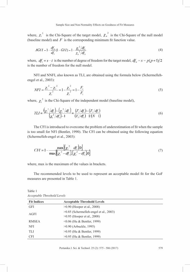
where, 2tχ is the Chi-Square of the target model,

2nχ is the Chi-Square of the null model

(baseline model) and F is the corresponding minimum fit function value.

(4)

where, is the number of degree of freedom for the target model, is the number of freedom for the null model.

NFI and NNFI, also known as TLI, are obtained using the formula below (Schermelleh-engel et al., 2003):

i

t

i

t

i

ti

FFNFI −=−=

−= 11 2

2

2

22

χχ

χχχ (5)

where, 2iχ is the Chi-Square of the independent model (baseline model),

(6)

The CFI is introduced to overcome the problem of underestimation of fit when the sample is too small for NFI (Bentler, 1990). The CFI can be obtained using the following equation (Schermelleh-engel et al., 2003):

(7)

where, max is the maximum of the values in brackets.

The recommended levels to be used to represent an acceptable model fit for the GoF measures are presented in Table 1.

Table 1Acceptable Threshold Levels

Fit Indices Acceptable Threshold LevelsGFI >0.90 (Hooper et al., 2008)

AGFI>0.85 (Schermelleh-engel et al., 2003)>0.95 (Hooper et al., 2008)

RMSEA <0.06 (Hu & Bentler, 1999)NFI >0.90 (Arbuckle, 1995)TLI >0.95 (Hu & Bentler, 1999)CFI >0.95 (Hu & Bentler, 1999)



SIMULATION DESIGN

This study investigated the performance of GoF measures under normal and non-normal conditions in SEM. Data were generated using a specified model given by Goodhue, Lewis, & Thompson (2012). The model included five constructs (one endogenous variable and four exogenous variables) with three indicators for each constructs. For each of the three indicators, standardised loading was fixed at 0.70, 0.80 and 0.90 respectively. Data was generated from Normal distribution N(0,1), and non-normal distributions which are Chi-Square distribution with 2 degrees of freedom, ( )22χ and Chi-Square distribution with 0.5 degrees of freedom,

( )5.02χ . The distribution of N(0,1) is a symmetric normal distribution, while ( )22χ and ( )5.02χ are skewed distribution with skewness of 2 and 4, respectively.For each data set, various sample sizes were considered to investigate their effect on GoF

measures, such as n= 100, 150, 200, 250, 300, 500, 1000, 1500 and 2000. The simulation involved 500 replications for each sample size and condition by using R, open source programming language. The minimum sample size of 100 was suggested by Hair Jr et al. (2010) for model containing constructs of less than six with indicators of more than three for each construct and possessing high item communalities (≥0.6). The theoretical model used in this study is shown in Figure 1.

Figure 1. Theoretical model - (Source: Goodhue, 2012)

RESULTS AND DISCUSSIONS

This section reports the results of GoF measures under normal and non-normal distributions. Box-plots were drawn to represent the GoF measures for various sample sizes under normal and non-normal conditions.

The performance of GoF measures for various sample sizes under normal and non-normal conditions are shown in Table 2. The GoF measures improved as the sample size



increased for all distributions. The TLI and CFI showed better fit compared with GFI and AGFI for all sample sizes. Thus, incremental fit measures were found to be less affected by sample sizes.

Table 2Mean of GoF measures

n GFI AGFI RMSEA NFI TLI CFI

a 100b100c100

0.9040.9020.903

0.8560.8530.855

0.0230.0280.026

0.8970.8960.898

0.9910.9860.990

0.9890.9860.986

a 150b150c150

0.9330.9320.933

0.9000.8990.900

0.0180.0200.019

0.9290.9280.930

0.9950.9940.995

0.9930.9920.992

a 200b200c200

0.9490.9490.949

0.9230.9230.924

0.0150.0150.015

0.9460.9460.947

0.9970.9960.997

0.9950.9950.994

a 250b250c250

0.9590.9590.959

0.9390.9390.938

0.0120.0130.013

0.9570.9570.957

0.9990.9980.998

0.9970.9960.996

a 300b300c300

0.9660.9650.966

0.9480.9480.948

0.0110.0110.011

0.9640.9640.964

0.9990.9990.999

0.9970.9970.997

a 500b500c500

0.9790.9790.979

0.9680.9680.969

0.0080.0080.008

0.9780.9780.978

0.9990.9991.000

0.9980.9980.998

a1000b1000c1000

0.9890.9890.989

0.9840.9840.984

0.0050.0060.006

0.9890.9890.989

1.0001.0001.000

0.9990.9990.999

a1500b1500c1500

0.9930.9930.993

0.9890.9890.989

0.0040.0040.004

0.9930.9930.993

1.0001.0001.000

0.9990.9990.999

a2000b2000c2000

0.9950.9950.995

0.9920.9920.992

0.0040.0040.004

0.9940.9940.994

1.0001.0001.000

1.0001.0001.000

Note: aNormal N(0,1) bChi-Square (2) cChi-Square (0.5)



The results in Table 2 were represented in box-plots as shown in Figure 2 for comparison purpose. Only the box-plot for GFI, RMSEA, TLI and CFI measures were presented because the pattern for AGFI and NFI measures were found to be similar with GFI.

Results show that GFI and AGFI are affected by sample size. These results contradicted the findings of Joreskog & Sorbom (1982) and Bagozzi & Yi (1988) who reported that GFI and AGFI are independent of sample size. However, our results confirm the findings of Fan, Thompson, & Wang (1999) who reported that GFI and AGFI are overly affected by sample size. GFI and AGFI are found to be robust against non-normality and these results are consistent with the findings by Joreskog & Sorbom (1982) and Bagozzi & Yi (1988). The behaviour of NFI is similar to GFI and AGFI.

Figure 2(a). Boxplots for GFI

Figure 2(b) and Figure 2(c) show the results of RMSEA and TLI for various sample sizes under normal and non-normal conditions. The boxplot (Figure 2(b)) shows that RMSEA is affected by sample size and less affected by non-normality when sample size is large. Figure 2(c) shows that TLI is less affected by sample size and this result supports the findings of Fan et al. (1999). However, TLI is not affected by distribution of data. According to Bentler (1990), TLI is difficult to interpret since the value can exceed the range (0-1).

Figure 2(b). Boxplots for RMSEA



Figure 2(c). Boxplots for TLI

Figure 2(d) displays the performance of CFI for various sample sizes under normal and non-normal conditions. The boxplot show that CFI is less affected by sample size and this result supports the findings of Fan et al. (1999). CFI is also less affected by distribution of data.

Figure 2(d). Boxplots for CFI

These boxplots show that GoF measures improved with the increase in sample size as expected. However, the simulation results indicated that GoF measures are not severely affected if distributions are non-normal.

CONCLUSIONS

This simulation study compared the effect of sample size and distribution of data on GoF measures for SEM. We found that the incremental fit measures are less affected by sample size and when distribution of data is not normal. However, severe non-normality due to the presence of outliers might affect GoF for SEM. Future simulation study can investigate the GoF measures in the presence of outliers and when data is non-normal with high multivariate skewness and kurtosis.



REFERENCESArbuckle, J. L. (1995). Amos 17 User ’ s Guide (pp. 1995-2005). Chicago, IL: SmallWaters Corporation.

Bagozzi, R. R., & Yi, Y. (1988). On the Evaluation of Structural Equation Models. Journal of the Academy of Marketing Science, 16(1), 74–94.

Bandalos, D. L. (2002). The Effects of Item Parceling on Goodness-of-Fit and Parameter Estimate Bias in Structural Equation Modeling. Structural Equation Modeling, 9(1), 78–102.

Bearden, W. O., Sharma, S., & Teel, J. E. (1982). Sample Size Effects on Chi Square and Other Statistics Used in Evaluating Causal Models. Journal of Marketing Research, 19(4), 425–430.

Bentler, P. M. (1990). Comparative Fit Indexes in Structural Models. Psychological Bulletin, 107(2), 238–246.

Curran, P. J., West, S. G., Finch, J. F., Aiken, L., Bentler, P., & Kaplan, D. (1996). The Robustness of Test Statistics to Nonnormality and Specification Error in Confirmatory Factor Analysis. Psychological Methods, 1(l), 16–29.

Ding, L., Velicer, W. F., & Harlow, L. L. (1995). Effects of Estimation Methods, Number of Indicators per Factor, and Improper Solutions on Structural Equation Modeling Fit Indices. Structural Equation Modeling, 2(2), 119–144.

Fan, X., Thompson, B., & Wang, L. (1999). Effects of sample size, estimation methods, and model specification on structural equation modeling fit indexes. Structural Equation Modeling, 6(1), 56–83. doi:10.1080/10705519909540119

Fox, J. (2002). Structural Equation Models. Appendix to An R and S-PLUS Companion to Applied Regression, 1–20.

Goodhue, D. L., Lewis, W., & Thompson, R. (2012). Does PLS Have Advantages for Small Sample Size or Non-Normal Data? MIS Quarterly, 36(3), 981–A16.

Hair JR, J. F., Black, W. C., Babin, B. J., & Anderson, R. E. (2010). Multivariate Data Analysis (7th Ed.). Upper Saddle River, NJ: Pearson Prentice Hall.

Hooper, D., Coughlan, J., & Mullen, M. R. (2008). Structural Equation Modelling : Guidelines for Determining Model Fit. The Electronic Journal of Business Research Methods, 6(1), 53–60.

Hu, L., & Bentler, P. M. (1999). Cutoff criteria for fit indexes in covariance structure analysis: Conventional criteria versus new alternatives. Structural Equation Modeling: A Multidisciplinary Journal, 6(1), 1–55. doi:10.1080/10705519909540118

Iacobucci, D. (2010). Structural equations modeling: Fit Indices, sample size, and advanced topics. Journal of Consumer Psychology, 20(2010), 90–98. doi:10.1016/j.jcps.2009.09.003

Jannoo, Z., Yap, B. W., Auchoybur, N., & Lazim, M. A. (2014). The Effect of Nonnormality on CB-SEM and PLS-SEM Path Estimates. International Journal of Mathematical, Computational, Physical and Quantum Engineering, 8(2), 285–291.

Joreskog, K. G., & Sorbom, D. (1982). Recent developments in structural equation modeling. Journal of Marketing Research, 19(4), 404–416.

Lei, P. W., & Wu, Q. (2007). Introduction to structural equation modeling: Issues and practical considerations. Educational Measurement: issues and practice, 26(3), 33-43.



Marsh, H. W., Balla, J. R., & McDonald, R. P. (1988). Goodness-of-Fit Indexes in Confirmatory Factor Analysis: The Effect of Sample Size. Psychological Bulletin, 103(3), 391–410. doi:10.1037//0033-2909.103.3.391

Mulaik, S. A., James, L. R., Alstine, J. Van, Bennett, N., Lind, S., & Stilwell, C. D. (1989). Evaluation of Goodness-of-Fit Indices for Structural Equation Models. Psychological Bulletin, 105(3), 430–445.

Rocha, C. M., & Chelladurai, P. (2012). Item Parcels in Structural Equation Modeling: an Applied Study in Sport Management. International Journal of Psychology and Behavioral Sciences, 2(1), 46–53. doi:10.5923/j.ijpbs.20120201.07

Schermelleh-engel, K., Moosbrugger, H., & Müller, H. (2003). Evaluating the Fit of Structural Equation Models : Tests of Significance and Descriptive Goodness-of-Fit Measures. Methods of Psychological Research Online, 8(2), 23–74.

Sharma, S., Mukherjee, S., Kumar, A., & Dillon, W. R. (2005). A simulation study to investigate the use of cutoff values for assessing model fit in covariance structure models. Journal of Business Research, 58(7), 935-943.

sample size and non-normality effects on goodness … papers/jst vol. 25 (2) apr. 2017...under...

Documents