sample papers and commentary

Nonlinear Casual Nexus between Stock Prices and Real Activity: Evidence from the Developed

Countries

Shyh-Wei Chena, Hsu-Wen Chenb

a Department of International Business, Center for Applied Economic Modeling,

Chung Yuan Christian University b Teaching and Learning Center, National Taipei University of Technology

___________________________________________________________________ Abstract: We examine the nexus of stock price changes and real economic activity for seven developed countries by using the vector error correction model, the bounds testing methodology, and linear and non-linear Granger causality methods. The empirical results substantiate that a long-run level equilibrium relationship exists among real activity and stock prices only for four of ten countries. The results from the linear Granger causality test indicate significant short-run and long-run causal relations between the stock price changes and real activity. In the results of the non-linear Granger causality, there are unidirectional and bidirectional non-linear causal relations between stock price changes and real output growth among these developed countries. Failure to allow for this non-linear property would lead to a misspecification of the relationship between real output growth and stock returns. JEL Classification: G1, O47, C32 Keywords: real activity, stock price, causality, non-linear, cointegration ___________________________________________________________________

1. Introduction

The relationship between stock price changes (or stock returns) and real economic activity is an important and interesting issue in the financial literature and has long been of interest to the public sector and academic circles alike. The interactions between the two sectors were first underlined by the q-theory of investment proposed by Brainard and Tobin (1968). They showed that capital

Vol 3, No.4, Winter 2011 Pages 93~121

IRABF 2011 Volume 3, Number 4

94

formation is triggered when the market value of new capital is higher than its replacement cost. Thus, there is a close link between output and asset markets.

According to the discounted-cash-flow valuation model, on the one hand, stock prices are essentially discounted expected future cash flows or earnings to be received by firms. Since firms’ earnings tend to be highly correlated with real income or real gross domestic product (GDP), it is believed that stock prices should reflect investors’ expectations about future real economic variables such as corporate earnings, or its aggregate proxy, real GDP. If these expectations are correct on average, lagged stock returns should be correlated with the contemporaneous growth rate of real GDP. That is, real stock price changes or returns should provide information about the future evolution of real GDP. Blanchard (1981) presented a standard IS-LM model that studies the effects of monetary and fiscal shocks on output, the stock market, and the term structure with gradual adjustment of output supply to demand shifts. In this framework, asset prices will tend to predict future output, but are not the cause of such changes, because both variables will tend to respond to changes in the economic environment. Empirically, if there is an unidirectional causality from stock price changes or returns to real activity, then we label it the stock returns-led real activity (SLA) hypothesis..

On the other hand, changes in real economic activity may also be useful to predict the evoluation of the stock market. For example, an exogenous rise in output or capital efficiency prompts a rise in private wealth and the value of equities leading to common movements in stock markets. Balvers et al. (1990) found that although lagged real stock returns significantly affect current real activity, current real activity, in turn, helps explain subsequent real stock returns. Empirically, unidirectional causality runs from real activity to stock price changes or returns and we label it the real activity-led stock returns (ALS) hypothesis.1

The third possible relationship between stock price changes and real economic activity is that there is bidirectional causal (feedback) between the two sectors. For example, Hassapis and Kalyvitis (2002a) develop a simple growth model that illustrates the relationship between stock price changes and output growth. They

1 Mrock et al. (1990) and Mauro (2003) review five existing theories of stock returns-real activity nexus in this literature. The theories may be grouped into those according to which stock price movements not reflecting changes in future “fundamentals” cannot predict changes in output (the “passive informant” hypothesis and the “accurate active informant” hypothesis), and those according to which they can (the “faulty active informant”, the “financing” hypothesis, and the “stock market pressure on managers” hypothesis). Readers are referred to their papers for detail.

Nonlinear Casual Nexus between Stock Prices and Real Activity: Evidence from the Developed Countries

95

show that in the context of this growth model there exists a positive relationship between stock prices and future growth (the SLA hypothesis hold). In addition, the model shows that there is a negative relationship between output growth and future stock returns (the ALS hypothesis hold).

Finally, as for the finding of no causality in either direction, this, the so-called neutral relationship, would signify that stock returns do not affect real activity and vice versa. A possible explanation of the omission of the relation of the stock market and real activity is the deviation of stock prices from fundamental values due to irrational exuberance or the emergence of speculative bubbles (Shiller, 2000).

On the empirical front, a substantial volume of studies have examined the stock prices or stock returns-real activity linkages, especially in the developed countries. Goldsmith (1969) was the first one who assessed the positive relationship between stock returns and economic growth. Subsequent work by Fama (1981, 1990), Schwert (1990), Barro (1990), Lee (1992) Gallinger (1994), Binswanger (2000), Gallegati (2008) confirmed that real stock returns are highly correlated with future real activity in the USA. These results hold for all data frequencies covering very long periods and are robust to alternative definitions of the data series. Also, a myriad of studies has investigated the stock returns-real activity relationship for other international markets (G-7, European countries and emerging markets). See, for example, Canova and Nicolo (1995), Peiro (1996), Cheung and Ng (1998), Kwon and Shin (1999), Choi et al. (1999), Aylward and Glen (2000), Hassapis and Kalyvitis (2002a,b), Mauro (2003), Chaudhuri and Smiles (2004), Binswanger (2004), Huang and Yang (2004), Silverstovs and Duong (2006) and Merikas and Merika (2006), Shen and Lin (2006), Shen and Lin (2009) and Shen et al. (2010).

But, unfortunately, studies such as these have borne the brunt of a great deal of criticism for three reasons. First, the findings from many previous studies have been mixed and, for the most part, do not reach a consensus as to the causal relationship between stock returns and real activity. Second, the causal models in these studies may very well have been misspecified on account of the fact that the traditional Granger (1969) causality F-test in a regression context may not be valid if the variables in the system are integrated, since the test statistic does not have a standard distribution (Toda and Phillips, 1995). Third, the majority overlooks the non-linear property inherent in goods market (e.g, expansion and contraction of the business cycle) and stock market (e.g., leverage effect and bull and bear markets) but only apply the traditional method in testing for the Granger causality of stock prices and


96

real GDP. Therefore, recent studies such as Domian and Louton (1997), Silvapulle, Silvapulle and Tan (1999), Alyward and Glen (2000), Sarantis (2001), Hassapis (2003), Henry, Olekalns and Thong (2004) and Chen, Lee and Wong (2006) allow for the possible non-linear relationship between stock returns and real activity.

In keeping with previous literature, the aim of this paper is to determine whether there is a non-linear causal relation in stock prices-real activity nexus for seven developed countries. The methodology used in this study differs from that in earlier studies in three ways.

First, by it very nature, the stock prices-real activity nexus is a long-run behavior relationship whose analysis requires methodologies appropriate for estimating long-run equilibrium. Therefore, we apply more advanced unit root and cointegration techniques, which account for a structural break, to avoid the potential estimation bias. We model the long-run relationship based on Pesaran's et al. (PSS, 2001) bounds test approach, and we extract critical values from Narayan (2005) and Turner (2006) specific to small samples. The advantages of the bounds test for cointegration are that (i) it can be applied to models consisting of variables with order of integration less or equal to one, and (ii) it can distinguish dependent from independent variables.

Second, we adopt Gregory and Hansen's (GH, 1996) residual-based test for cointegration with regime shifts. GH's (1996) method is unique in the sense that it allows practitioners to conduct a test for cointegration among variables in the presence of structural shifts.

Third, we do not assume that the nexus between output growth and stock return is linear since the non-linear property inherent in goods market (e.g, expansion and contraction of the business cycle) and stock market (e.g., leverage effect and bull and bear markets) could result in a nonlinear relationship between the two sectors. In order to characterize this feature, in addition to the linear Granger causality (GC) test, we employ Hiemstra and Jones' (HJ, 1994) non-linear method and Diks and Panchenko's (DP, 2006) modified non-parametric method which enables us to test for non-linear Granger causality, and at the same time avoid making spurious inferences. The empirical investigation also enables us to identify which hypothesis is most applicable to these developed countries. The evidence gained from the empirical work on the lead-lag relation helps us determine the suitability of the theoretical explanation.


97

The organization of the paper is as follows. Section 2 introduces the econometric methodology that we employ. We describe the data and discuss the empirical test results as well as compare results with previous findings in Section 3. Section 4 discusses the conclusions and implications that we draw from this research.

2. Methodology

2.1 Bounds Test Approach

Pesaran et al. (2001) developed the bounds test procedure based on the AutoRegressive Distributed Lag (ARDL) model, and in the case of small samples, its performance is superior to that of other estimators (see Pesaran and Shin, 1995). More specifically, when written in the Error Correction model (ECM) form, the ARDL model is much less vulnerable to spurious regression (Pesaran and Smith, 1998). All of the variables used are in natural logarithms.

Pesaran et al. (2001) considered five models to conduct the bounds test. Let ' '( , )t t tz y x , where ty is dependent variable and tx is a vetor of independent

variables.

Case I (no intercept and no trend)

Case II (restricted intercept and no trend)

Case III (unrestricted intercept and no trend)

Case IV (unrestricted intercept and restricted trend)

Case V (unrestricted intercept and unrestricted trend)

'1 . 1

1 0

p q

t yy t yx x t i t i t j t yti j

y y x y x

'1 . 1

1 0

( )p q

t yy t y yx x t i t i t j t yti j

y y x y x

'0 1 . 1

1 0

p q


y y x y x

'0 1 . 1

1 0

( ) ( )p q

t yy t y yx x t x i t i t j t yti j

y y t x t y x


98

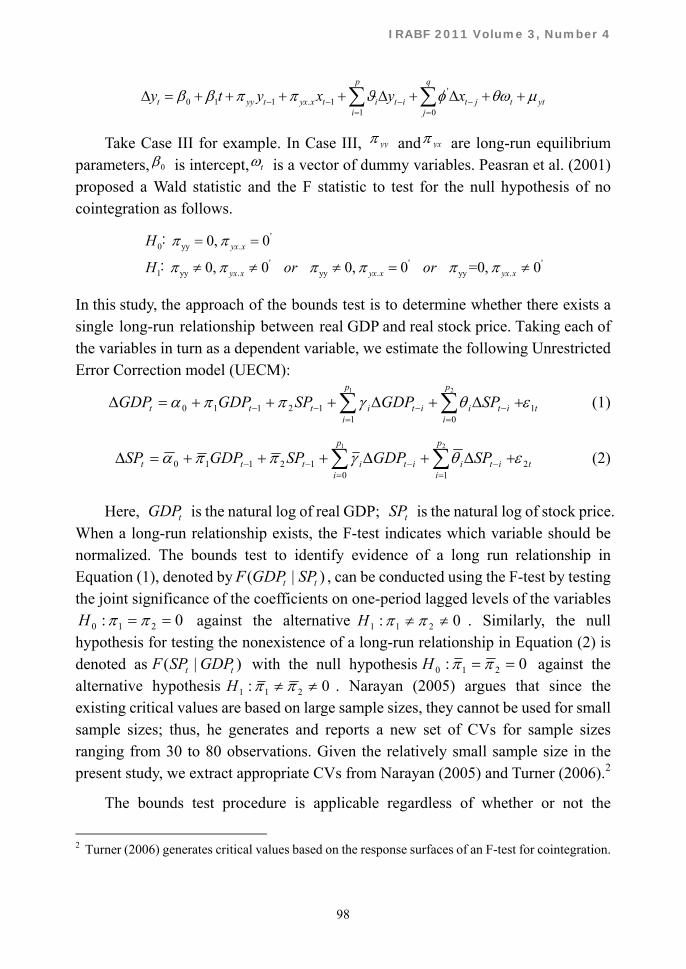
Take Case III for example. In Case III, yy and yx are long-run equilibrium parameters, 0 is intercept, t is a vector of dummy variables. Peasran et al. (2001) proposed a Wald statistic and the F statistic to test for the null hypothesis of no cointegration as follows.

In this study, the approach of the bounds test is to determine whether there exists a single long-run relationship between real GDP and real stock price. Taking each of the variables in turn as a dependent variable, we estimate the following Unrestricted Error Correction model (UECM):

t

p

i

p

iitiitittt SPGDPSPGDPGDP 1

1 012110

1 2

(1)

t

p

i

p

iitiitittt SPGDPSPGDPSP 2

0 112110

1 2

(2)

Here, tGDP is the natural log of real GDP; tSP is the natural log of stock price. When a long-run relationship exists, the F-test indicates which variable should be normalized. The bounds test to identify evidence of a long run relationship in Equation (1), denoted by )|( tt SPGDPF , can be conducted using the F-test by testing the joint significance of the coefficients on one-period lagged levels of the variables

0: 210 H against the alternative 0: 211 H . Similarly, the null hypothesis for testing the nonexistence of a long-run relationship in Equation (2) is denoted as )|( tt GDPSPF with the null hypothesis 0: 210 H against the alternative hypothesis 0: 211 H . Narayan (2005) argues that since the existing critical values are based on large sample sizes, they cannot be used for small sample sizes; thus, he generates and reports a new set of CVs for sample sizes ranging from 30 to 80 observations. Given the relatively small sample size in the present study, we extract appropriate CVs from Narayan (2005) and Turner (2006).2

The bounds test procedure is applicable regardless of whether or not the

2 Turner (2006) generates critical values based on the response surfaces of an F-test for cointegration.

'0 1 1 . 1

1 0

p q


y t y x y x

'0 .

' ' '1 . . .

0, 0

0, 0 0, 0 =0, 0

yx x

yx x yx x yx x

H

H or or

yy

yy yy yy

：

：


99

underlying regressors are integrated on the order of one or zero, or are mutually cointegrated. The ARDL regression, on the other hand, yields a test statistic which can be compared to two asymptotic critical values. When the test statistic is greater than a certain upper critical value, the null hypothesis of a no long-run relationship must be rejected whether or not the underlying orders of integration of the regressors are zero or one. Alternatively, when the test statistic is less than a certain lower critical value, the null hypothesis of a no long-run relationship between the regressors cannot be rejected. If the test statistic falls between these two bounds, the results are deemed unknown.

2.2 Gregory and Hansen's (1996) Tests for Cointegration

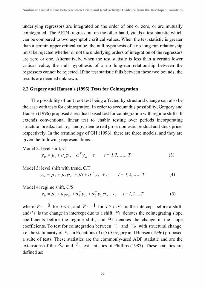
The possibility of unit root test being affected by structural change can also be the case with tests for cointegration. In order to account this possibility, Gregory and Hansen (1996) proposed a residual-based test for cointegration with regime shifts. It extends conventional linear test to enable testing over periods incorporating structural breaks. Let ty1 and ty2 denote real gross domestic product and stock price, respectively. In the terminology of GH (1996), there are three models, and they are given the following representations:

Model 2: level shift, C

ttT

tt eyy 2211 t = 1,2,……,T (3)

Model 3: level shift with trend, C/T tt

Ttt eyty 2211 t = 1,2,……,T (4)

Model 4: regime shift, C/S

tttT

tT

tt eyyy 2221211 t =1,2,...,T (5)

where 0t for t , and 1t for t . 1 is the intercept before a shift, and 2 is the change in intercept due to a shift. 1 denotes the cointegrating slope coefficients before the regime shift, and 2 denotes the change in the slope coefficients. To test for cointegration between ty1 and ty2 with structural change, i.e. the stationarity of te in Equations (3)-(5). Gregory and Hansen (1996) proposed a suite of tests. These statistics are the commonly-used ADF statistic and are the extensions of the Z and tZ test statistics of Phillips (1987). These statistics are defined as:


100

)(inf* ZZ

)(inf* tt ZZ

)(inf* ADFADF

If the break point is unknown a priori, the model is estimated recursively allowing the break point to vary such that |0.15T| |0.85T|, where T is the sample size. The statistics of interest are the smallest values of all of the above statistics across all values of T. We examine the smallest values since the smallest values of the test statistics constitute evidence against the null hypothesis.

2.3 Granger Causality Test

In order to determine the causal relationships, in the presence of cointegration, Granger causality requires the inclusion of an error correction term in the stationary model to capture the short-run deviations of the series from their long-run equilibrium path. The ECM-VAR model, that is, when the error correction term is added to Eqs. (1)-(2), is estimated, and the Granger causality test is employed. The equations are written as follows:

t

k

it

k

iitiitit ECTSPGDPGDP 1

111

10

(3)

t

k

i

k

ititiitit ECTSPGDPSP 2

1 1120

(4)

All variables are as previously defined. t1 and t2 are error terms that are assumed to be white noise with zero mean, constant variance and no autocorrelation. In Equation (3), for example, the SLA hypothesis is confirmed either if the short-term causality, i.e., tSP does not ‘Granger-cause’ tGDP if and only if

ii 0 , or if the long-run non-causality, through the lagged error correction term, i.e., 01 , is rejected at the 5% level. Likewise, the ALS hypothesis is confirmed either if the short-term causality, i.e., tGDP does not ‘Granger-cause’ tSP if and only if ii 0 , or if the long-run non-causality, through the lagged error correction term, i.e., 02 , is rejected at the 5% level.


101

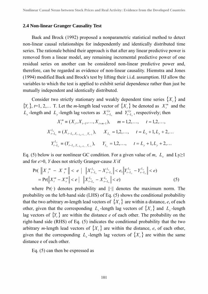
2.4 Non-linear Granger Causality Test

Baek and Brock (1992) proposed a nonparametric statistical method to detect non-linear causal relationships for independently and identically distributed time series. The rationale behind their approach is that after any linear predictive power is removed from a linear model, any remaining incremental predictive power of one residual series on another can be considered non-linear predictive power and, therefore, can be regarded as evidence of non-linear causality. Hiemstra and Jones (1994) modified Baek and Brock's test by lifting their i.i.d. assumption. HJ allow the variables to which the test is applied to exhibit serial dependence rather than just be mutually independent and identically distributed.

Consider two strictly stationary and weakly dependent time series tX and tY , t=1, 2,… T. Let the m-length lead vector of tX be denoted as m

tX and the

xL -length and yL -length lag vectors as LxLt x

X and LyLt y

Y , respectively; then

mtX ),,,,( 11 mttt XXX ,,2,1 m ,,2,1 t

x

x

LLtX ),(

1,,1, txLtx XXLtX

,,2,1 xLX ,2,1 xx LLt

y

y

L

LtY ),(1,,1, txLty YYLtY

,,2,1

yLY ,2,1 yy LLt

Eq. (5) below is our nonlinear GC condition. For a given value of m, xL and Ly≥1 and for e>0, Y does not strictly Granger-cause X if

eXX ms

mt Pr( ), eYYeXX y

y

y

y

x

x

x

x

L

Ls

L

LtL

LsL

Lt

eXX ms

mt Pr( )eXX x

x

x

x

LLs

LLt (5)

where Pr(·) denotes probability and ||·|| denotes the maximum norm. The probability on the left-hand side (LHS) of Eq. (5) shows the conditional probability that the two arbitrary m-length lead vectors of tX are within a distance, e, of each other, given that the corresponding xL -length lag vectors of tX and yL -length lag vectors of tY are within the distance e of each other. The probability on the right-hand side (RHS) of Eq. (5) indicates the conditional probability that the two arbitrary m-length lead vectors of tX are within the distance, e, of each other, given that the corresponding xL -length lag vectors of tX are within the same distance e of each other.

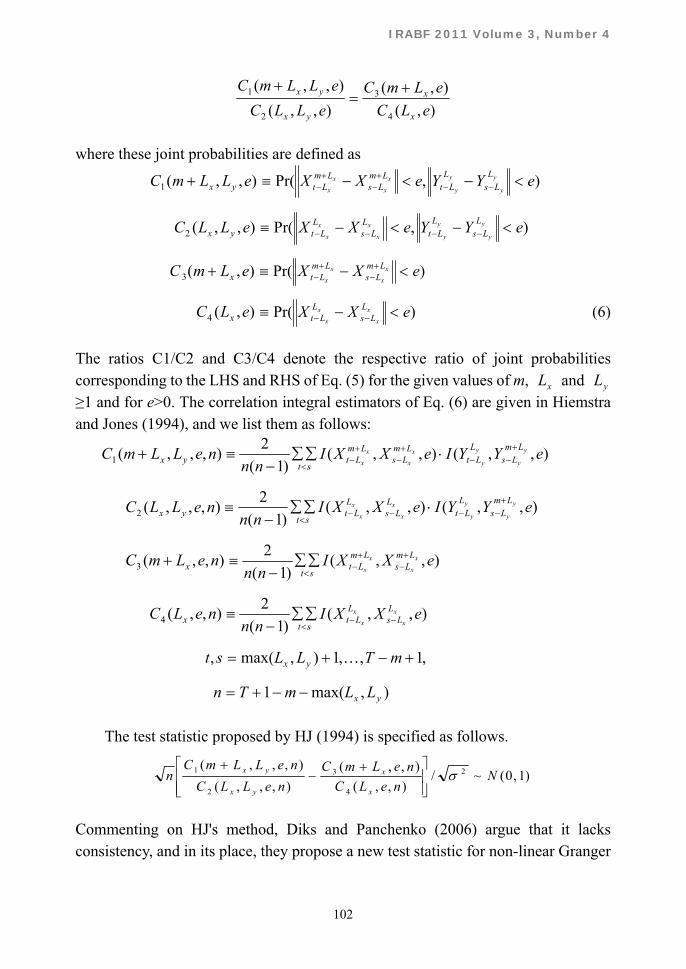
Eq. (5) can then be expressed as


102

),(

),(

),,(

),,(

4

3

2

1

eLC

eLmC

eLLC

eLLmC

x

x

yx

yx

where these joint probabilities are defined as

),,(1 eLLmC yx ),Pr( eYYeXX y

y

y

y

x

x

x

x

L

Ls

L

LtLm

LsLm

Lt

),,(2 eLLC yx ),Pr( eYYeXX y

y

y

y

x

x

x

x

L

Ls

L

LtL

LsL

Lt

),(3 eLmC x )Pr( eXX x

x

x

x

LmLs

LmLt

),(4 eLC x )Pr( eXX x

x

x

x

LLs

LLt (6)

The ratios C1/C2 and C3/C4 denote the respective ratio of joint probabilities corresponding to the LHS and RHS of Eq. (5) for the given values of m, xL and yL≥1 and for e>0. The correlation integral estimators of Eq. (6) are given in Hiemstra and Jones (1994), and we list them as follows:

),,,(1 neLLmC yx ),,(),,()1(

2eYYIeXXI

nny

y

y

y

x

x

x

x

Lm

Ls

L

LtLm

LsLm

Ltst

),,,(2 neLLC yx ),,(),,()1(

2eYYIeXXI

nny

y

y

y

x

x

x

x

LmLs

LLt

LLs

LLt

st

),,(3 neLmC x ),,()1(

2eXXI

nnx

x

x

x

LmLs

LmLt

st

),,(4 neLC x ),,()1(

2eXXI

nnx

x

x

x

LLs

LLt

st

st, ,1,,1),max( mTLL yx

n ),max(1 yx LLmT

The test statistic proposed by HJ (1994) is specified as follows.

)1 ,0(~/),,(

),,(

),,,(

),,,(2

4

3

2

1 NneLC

neLmC

neLLC

neLLmCn

x

x

yx

yx

Commenting on HJ's method, Diks and Panchenko (2006) argue that it lacks consistency, and in its place, they propose a new test statistic for non-linear Granger


103

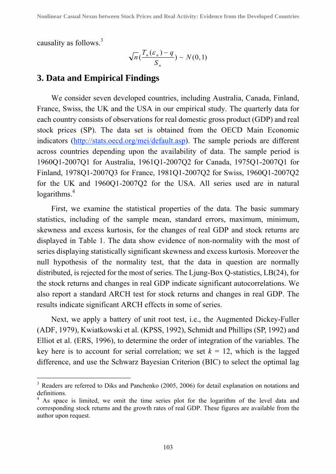
causality as follows.3

)1 ,0(~))(

( NS

qTn

n

nn

3. Data and Empirical Findings

We consider seven developed countries, including Australia, Canada, Finland, France, Swiss, the UK and the USA in our empirical study. The quarterly data for each country consists of observations for real domestic gross product (GDP) and real stock prices (SP). The data set is obtained from the OECD Main Economic indicators (http://stats.oecd.org/mei/default.asp). The sample periods are different across countries depending upon the availability of data. The sample period is 1960Q1-2007Q1 for Australia, 1961Q1-2007Q2 for Canada, 1975Q1-2007Q1 for Finland, 1978Q1-2007Q3 for France, 1981Q1-2007Q2 for Swiss, 1960Q1-2007Q2 for the UK and 1960Q1-2007Q2 for the USA. All series used are in natural logarithms.4

First, we examine the statistical properties of the data. The basic summary statistics, including of the sample mean, standard errors, maximum, minimum, skewness and excess kurtosis, for the changes of real GDP and stock returns are displayed in Table 1. The data show evidence of non-normality with the most of series displaying statistically significant skewness and excess kurtosis. Moreover the null hypothesis of the normality test, that the data in question are normally distributed, is rejected for the most of series. The Ljung-Box Q-statistics, LB(24), for the stock returns and changes in real GDP indicate significant autocorrelations. We also report a standard ARCH test for stock returns and changes in real GDP. The results indicate significant ARCH effects in some of series.

Next, we apply a battery of unit root test, i.e., the Augmented Dickey-Fuller (ADF, 1979), Kwiatkowski et al. (KPSS, 1992), Schmidt and Phillips (SP, 1992) and Elliot et al. (ERS, 1996), to determine the order of integration of the variables. The key here is to account for serial correlation; we set k = 12, which is the lagged difference, and use the Schwarz Bayesian Criterion (BIC) to select the optimal lag

3 Readers are referred to Diks and Panchenko (2005, 2006) for detail explanation on notations and definitions. 4 As space is limited, we omit the time series plot for the logarithm of the level data and corresponding stock returns and the growth rates of real GDP. These figures are available from the author upon request.


104

length. In general, we find strong evidence in favor of the unit root hypothesis based on test results in their respective level data with minority is not. When we apply the unit root test to the first difference of these series, again, we are able to reject the null hypothesis of a unit root at the 5% level or better.5

Table 1 Descriptive Statistics

Country Variable Statistic

Mean S.D SK EK Max Min JB LB(24) ARCH(4)

Australia DGDP 0.009 0.012 0.141 0.957 0.045 -0.031 7.805** 52.887*** 2.538** DSP 0.018 0.082 -1.692 8.766 0.196 -0.489 691.657** 35.543 0.920

Canada DGDP 0.009 0.009 0.164 0.168 0.031 -0.016 1.038 63.185*** 2.993* DSP 0.017 0.070 -0.760 1.785 0.186 -0.264 42.130** 46.448*** 0.794

Finland DGDP 0.007 0.011 -0.013 2.169 0.049 -0.028 25.093*** 91.950*** 1.118 DSP 0.029 0.117 -0.157 0.910 0.417 -0.329 4.942 65.113*** 4.981***

France DGDP 0.005 0.005 0.245 -0.091 0.019 -0.007 1.224 71.099*** 3.833*** DSP 0.028 0.087 -0.776 2.061 0.227 -0.325 32.725** 47.128*** 0.048

Swiss DGDP 0.004 0.007 -0.043 -0.206 0.023 -0.010 0.218 39.552** 1.411 DSP 0.023 0.075 -1.391 4.557 0.161 -0.338 124.722*** 43.407*** 0.144

UK DGDP 0.006 0.010 0.759 4.939 0.056 -0.028 210.204*** 40.593** 0.927 DSP 0.019 0.079 -0.176 3.436 0.352 -0.271 93.947*** 42.791** 18.299***

USA DGDP 0.008 0.008 -0.121 1.046 0.039 -0.020 9.374*** 55.321*** 1.471 DSP 0.018 0.058 -0.629 2.101 0.187 -0.224 47.241** 53.329** 1.437

(1)*, ** and *** denote significant at the 10%, 5% and 1% levels, respectively (2) Mean and S.D. refer to the mean and standard deviation of the returns on each market, Max is the largest observation, and Min is the smallest observation.

(3) SK is the skewness coefficient. (4) EK is the excess kurtosis coefficient. (5) JB is the Jarque-Bera statistic. (6) LB(24) is the Ljung-Box Q statistic, calculated with 24 lags, for raw returns. (7) ARCH(4) is the ARCH test, calculated with 4 lags, for residuals from an AR(4) regression on raw returns. (8) DGDP and DSP denote the changes of real GDP and stock return, respectively.

Perron (1989) pointed out, in the presence of a structural break, the power to reject a unit root decreases if the stationary alternative is true and the structural break is ignored. To address this, we use of Zivot and Andrews’ (ZA, 1992) sequential trend break models to investigate the order of the empirical variables. The results suggest that stock prices are non-stationary in their respective levels. 6 These

5 The results of unit root tests for the level data and first-differenced data are omitted due to space constraint and they are available from the author upon request. 6 ZA (1992) warned that with small sample sizes, the distribution of the test statistic can deviate substantially from those with asymptotic distribution. In general, the critical values for small samples are smaller (more negative) than those with asymptotic distribution. Because our test results are larger than the asymptotic critical values, we believe that our conclusions are unchanged if we use the small sample critical values.


105

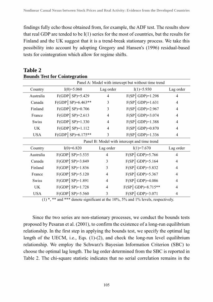
findings fully echo those obtained from, for example, the ADF test. The results show that real GDP are tended to be I(1) series for the most of countries, but the results for Finland and the UK suggest that it is a trend-break stationary process. We take this possibility into account by adopting Gregory and Hansen's (1996) residual-based tests for cointegration which allow for regime shifts.

Table 2 Bounds Test for Cointegration

Panel A: Model with intercept but without time trend

Country I(0)=5.060 Lag order I(1)=5.930 Lag order

Australia F(GDP│SP)=5.429 4 F(SP│GDP)=1.298 4

Canada F(GDP│SP)=6.463** 3 F(SP│GDP)=1.631 4

Finland F(GDP│SP)=0.706 3 F(SP│GDP)=2.967 4

France F(GDP│SP)=2.613 4 F(SP│GDP)=3.074 4

Swiss F(GDP│SP)=1.330 4 F(SP│GDP)=1.388 4

UK F(GDP│SP)=1.112 4 F(SP│GDP)=0.870 4

USA F(GDP│SP)=6.175** 3 F(SP│GDP)=1.336 4

Panel B: Model with intercept and time trend

Country I(0)=6.820 Lag order I(1)=7.670 Lag order

Australia F(GDP│SP)=3.535 4 F(SP│GDP)=5.766 4

Canada F(GDP│SP)=3.849 3 F(SP│GDP)=5.164 4

Finland F(GDP│SP)=1.836 3 F(SP│GDP)=5.832 4

France F(GDP│SP)=5.120 4 F(SP│GDP)=5.367 4

Swiss F(GDP│SP)=1.891 4 F(SP│GDP)=4.086 4

UK F(GDP│SP)=1.728 4 F(SP│GDP)=8.715** 4

USA F(GDP│SP)=5.560 3 F(SP│GDP)=3.071 4

(1) *, ** and *** denote significant at the 10%, 5% and 1% levels, respectively.

Since the two series are non-stationary processes, we conduct the bounds tests proposed by Pesaran et al. (2001), to confirm the existence of a long-run equilibrium relationship. In the first step in applying the bounds test, we specify the optimal lag length of the UECM, i.e., Eqs. (1)-(2), and check the long-run level equilibrium relationship. We employ the Schwarz's Bayesian Information Criterion (SBC) to choose the optimal lag length. The lag order determined from the SBC is reported in Table 2. The chi-square statistic indicates that no serial correlation remains in the


106

residual when the lag length is chosen.7 Here, we conduct the bounds tests (without and with trend) to confirm the existence of a long-run equilibrium relationship among stock prices and real GDP, and we report the results in Table 2. Worth noting is that due to the relatively mediate sample size in the present study, we extract the critical values from Narayan (2005).

3.1 Estimation results of long-run equilibrium

The bounds test procedure is applicable irrespective of whether the underlying regressors are integrated on the order of one or zero, or are mutually cointegrated. By contrast, the ARDL regression yields a test statistic which can be compared to two asymptotic critical values. If the test statistic is above a certain upper critical value, the null hypothesis of a no long-run relationship must be rejected regardless of whether the underlying orders of integration of the regressors are zero or one. Alternatively, if the test statistic falls below a certain lower critical value, the null hypothesis of a no long-run relationship between the regressors cannot be rejected. If the test statistic falls between these two bounds, the results are, in a word, inconclusive.

It is clear that, in the case of Canada, if the GDP is used as the dependent variable, then the computed F-statistic (without trend, 463.6)( SPGDPF ) exceeds the upper critical value (I(1)=5.930). If stock price is used as the dependent variable, then the computed F-statistic ( )( GDPSPF =1.631) is smaller than the lower critical value (I(0)=5.060) and it is insignificant at the 5% level. This substantiates that the null hypothesis of no level long-run relationship must be rejected and, moreover, the dependent variable should be real GDP. But this does not rule out a short-run relationship between real GDP and stock prices.

We reach a same conclusion for the USA, that is, there is a long-run level equilibrium relationship between stock prices and real GDP and dependent variable is real GDP. However, we cannot find the long-run level relationships between stock prices and real GDP for Australia, Finland, France, Swiss and the UK.

With a time trend model, the F test suggests that the null hypothesis of no

7 As noted by PSS (2001, p312), “in testing the null hypothesis of the absence of the level long-run relationship in Eq. (1)-(2), it is important that the coefficients of the lagged change remain unrestricted; otherwise, these tests could be subject to a pre-testing problem. However, for the subsequent estimations of the level effects and short-run dynamics of the adjustments, the use of more parsimonious specifications seems advisable.”


107

long-run relationship between the real GDP and stock prices cannot be rejected at the 5% significant level for all countries except the UK. Because the bounds test with a time trend does not change the main results of the bounds test without a time trend, therefore we proceed to conduct the Granger causality test without a time trend. Moreover, the robustness of the ARDL model with respective to the Johansen and Juselius (1990) method is also checked and the estimated results from the two methods are quite alike, therefore, we omit the detail.8

Table 3 Results from the Gregory and Hansen Cointegration test (GDP is dependent variable)

Country Model Statistic

ADF* Tb Z*t Tb

*Z Tb

Australia

C -3.806 1968Q1 -3.640 1971Q4 -22.378 1971Q4

C/T -3.661 1967Q1 -3.612 1967Q4 -24.203 1967Q4

C/S -4.239 1972Q1 -3.842 1971Q4 -26.175 1972Q1

Canada

C -4.644** 1971Q2 -4.170 1970Q1 -30.361 1970Q1

C/T -4.083 1991Q1 -4.240 1991Q1 -26.569 1991Q1

C/S -5.620** 1975Q1 -5.158** 1974Q4 -48.439** 1974Q4

Finland

C -4.278 2002Q2 -3.175 2001Q4 -17.108 2001Q4

C/T -4.990** 1991Q2 -4.985 1991Q2 -40.236 1991Q2

C/S -4.287 2002Q1 -3.358 2001Q4 -18.644 2001Q4

France

C -3.559 2001Q4 -3.318 2001Q4 -20.498 2001Q3

C/T -3.303 1986Q2 -2.544 1989Q1 -12.501 1987Q1

C/S -3.482 2001Q4 -3.291 2001Q4 -20.131 2001Q4

Swiss

C -2.210 1995Q1 -2.109 2003Q2 -8.103 2003Q2

C/T -3.695 1986Q1 -2.928 1994Q2 16.497 1994Q2

C/S -2.181 1993Q4 -2.087 2003Q2 -7.905 2003Q2

UK

C -3.078 1983Q1 -2.957 2000Q2 -14.646 1983Q1

C/T -4.561 1978Q1 -3.649 1979Q3 -24.505 1979Q3

C/S -3.284 1981Q1 -2.993 1981Q2 -17.021 1981Q2

USA

C -4.535 1971Q3 -3.772 1970Q4 -25.426 1970Q4

C/T -4.950 1967Q3 -3.663 1966Q4 -25.848 1996Q4

C/S -5.845** 1973Q3 -5.095** 1974Q3 -47.461** 1974Q3


8 As space is limited, we do not show the Johansen’s test results. The table is available from the author upon request.


108

Table 4 Results from the Gregory and Hansen Cointegration test (SP is dependent variable)

Country Model Statistic

ADF* Tb Z*t Tb

*Z Tb

Australia C -3.813 1969Q2 -3.425 1971Q4 -23.263 1984Q2

C/T -4.446 1972Q3 -3.803 1972Q2 -27.131 1972Q2 C/S -4.941 1981Q3 -4.407 1984Q1 -31.240 1984Q1

Canada C -4.393 1971Q2 -3.906 1970Q4 -27.406 1970Q2

C/T -4.644 1972Q2 -4.103 1990Q4 -32.464 1990Q4 C/S -5.438** 1979Q1 -4.934 1979Q1 -46.073 1979Q1

Finland C -4.055 2002Q2 -2.941 2001Q4 -15.375 2001Q4

C/T -4.281 2002Q2 -3.075 2001Q4 -16.166 2001Q4 C/S -4.518 1997Q4 -3.112 1998Q2 -17.945 1998Q1

France C -3.951 1984Q3 -3.607 1984Q3 -23.717 1984Q3

C/T -3.972 1984Q3 -6.588 1984Q3 -23.582 1984Q3 C/S -3.863 1984Q3 -3.449 2001Q4 -21.772 1984Q2

Swiss C -3.376 1995Q1 -2.894 1994Q3 -16.231 1994Q3

C/T -3.350 2001Q4 -3.154 2001Q4 -18.343 2001Q4 C/S -3.429 1995Q1 -2.976 1996Q2 -17.316 1996Q2

UK C -3.743 1983Q1 -3.541 1983Q2 -23.632 1983Q2

C/T -4.398 1984Q4 -3.850 1985Q2 -27.786 1985Q2 C/S -3.750 1981Q3 -3.527 1981Q3 -24.299 1981Q3

USA C -4.192 1971Q3 -3.529 1970Q3 -22.754 1970Q4

C/T -4.396 1971Q3 -3.807 1972Q3 -26.860 1972Q2 C/S -4.858 1974Q4 -4.352 1974Q4 -35.663 1974Q4


The Gregory and Hansen test results for cointegration in models with regime shift are presented in Table 3 (using real GDP as dependent variable) and 4 (using stock price as dependent variable). The GH test is a residual-based test, which test the null hypothesis of no cointegration against the alternative of cointegration in the presence of a possible regime shift. The test results suggest that the null hypothesis of no cointegration is rejected for the case of Canada, Finland and the USA. The test results, in general, corroborate those from the bounds testing approach. Thus, there is compelling evidence of cointegration between the real GDP and stock prices both with and without regime change in Canada, Finland and the USA.

3.2 Results of lnear Granger causality

To check the causal relationship, we estimate a vector autoregressive (VAR) model for the Australia, France, Swiss and the UK because the null hypothesis of no cointegration is not rejected from the results of the ARDL, Johansen and GH tests. But we estimate an error correction model for Canada, Finland and the USA because there is a long-run relationship between stock prices and real GDP based on the


109

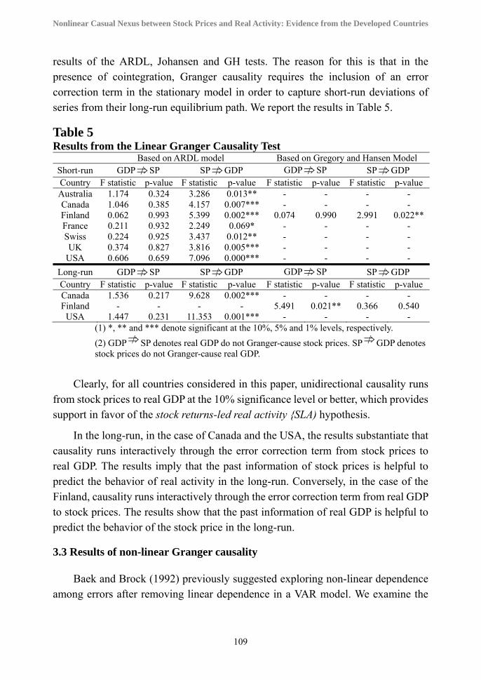
results of the ARDL, Johansen and GH tests. The reason for this is that in the presence of cointegration, Granger causality requires the inclusion of an error correction term in the stationary model in order to capture short-run deviations of series from their long-run equilibrium path. We report the results in Table 5.

Table 5 Results from the Linear Granger Causality Test

Based on ARDL model Based on Gregory and Hansen Model Short-run GDP SP SP GDP GDP SP SP GDP Country F statistic p-value F statistic p-value F statistic p-value F statistic p-value Australia 1.174 0.324 3.286 0.013** - - - - Canada 1.046 0.385 4.157 0.007*** - - - - Finland 0.062 0.993 5.399 0.002*** 0.074 0.990 2.991 0.022** France 0.211 0.932 2.249 0.069* - - - - Swiss 0.224 0.925 3.437 0.012** - - - - UK 0.374 0.827 3.816 0.005*** - - - -

USA 0.606 0.659 7.096 0.000*** - - - -

Long-run GDP SP SP GDP GDP SP SP GDP Country F statistic p-value F statistic p-value F statistic p-value F statistic p-value Canada 1.536 0.217 9.628 0.002*** - - - - Finland - - - - 5.491 0.021** 0.366 0.540

USA 1.447 0.231 11.353 0.001*** - - - - (1) *, ** and *** denote significant at the 10%, 5% and 1% levels, respectively.

(2) GDP SP denotes real GDP do not Granger-cause stock prices. SP GDP denotes stock prices do not Granger-cause real GDP.

Clearly, for all countries considered in this paper, unidirectional causality runs from stock prices to real GDP at the 10% significance level or better, which provides support in favor of the stock returns-led real activity {SLA) hypothesis.

In the long-run, in the case of Canada and the USA, the results substantiate that causality runs interactively through the error correction term from stock prices to real GDP. The results imply that the past information of stock prices is helpful to predict the behavior of real activity in the long-run. Conversely, in the case of the Finland, causality runs interactively through the error correction term from real GDP to stock prices. The results show that the past information of real GDP is helpful to predict the behavior of the stock price in the long-run.

3.3 Results of non-linear Granger causality

Baek and Brock (1992) previously suggested exploring non-linear dependence among errors after removing linear dependence in a VAR model. We examine the


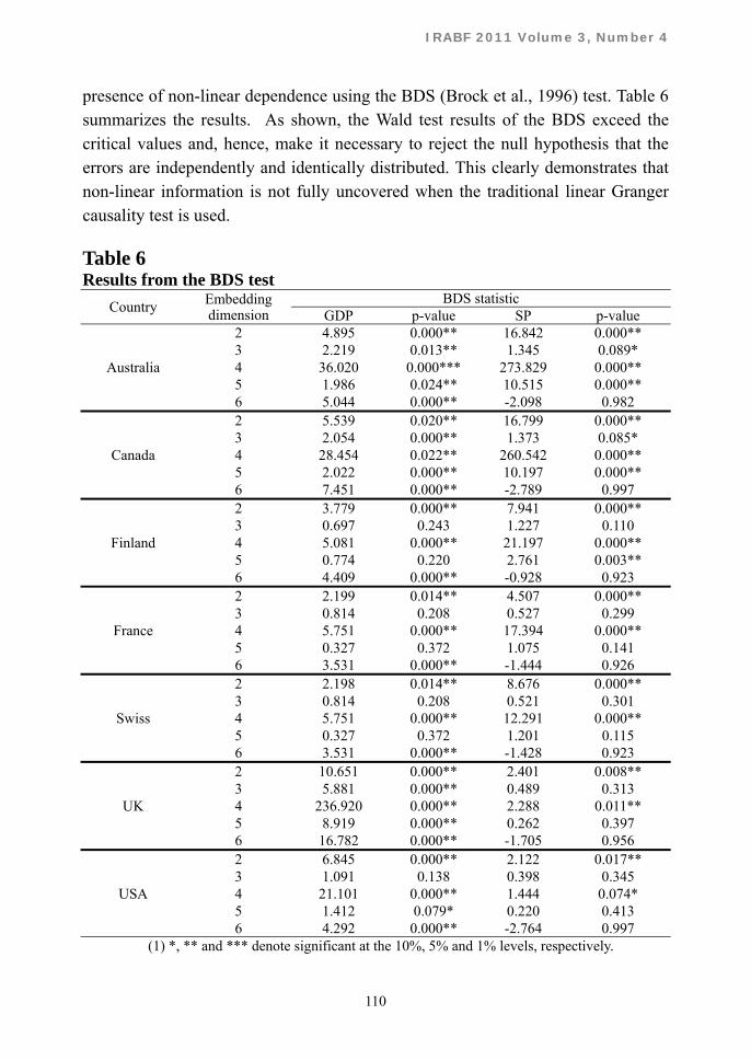
110

presence of non-linear dependence using the BDS (Brock et al., 1996) test. Table 6 summarizes the results. As shown, the Wald test results of the BDS exceed the critical values and, hence, make it necessary to reject the null hypothesis that the errors are independently and identically distributed. This clearly demonstrates that non-linear information is not fully uncovered when the traditional linear Granger causality test is used.

Table 6 Results from the BDS test

Country Embedding dimension

BDS statistic GDP p-value SP p-value

Australia

2 4.895 0.000** 16.842 0.000** 3 2.219 0.013** 1.345 0.089* 4 36.020 0.000*** 273.829 0.000** 5 1.986 0.024** 10.515 0.000** 6 5.044 0.000** -2.098 0.982

Canada

2 5.539 0.020** 16.799 0.000** 3 2.054 0.000** 1.373 0.085* 4 28.454 0.022** 260.542 0.000** 5 2.022 0.000** 10.197 0.000** 6 7.451 0.000** -2.789 0.997

Finland

2 3.779 0.000** 7.941 0.000** 3 0.697 0.243 1.227 0.110 4 5.081 0.000** 21.197 0.000** 5 0.774 0.220 2.761 0.003** 6 4.409 0.000** -0.928 0.923

France

2 2.199 0.014** 4.507 0.000** 3 0.814 0.208 0.527 0.299 4 5.751 0.000** 17.394 0.000** 5 0.327 0.372 1.075 0.141 6 3.531 0.000** -1.444 0.926

Swiss

2 2.198 0.014** 8.676 0.000** 3 0.814 0.208 0.521 0.301 4 5.751 0.000** 12.291 0.000** 5 0.327 0.372 1.201 0.115 6 3.531 0.000** -1.428 0.923

UK

2 10.651 0.000** 2.401 0.008** 3 5.881 0.000** 0.489 0.313 4 236.920 0.000** 2.288 0.011** 5 8.919 0.000** 0.262 0.397 6 16.782 0.000** -1.705 0.956

USA

2 6.845 0.000** 2.122 0.017** 3 1.091 0.138 0.398 0.345 4 21.101 0.000** 1.444 0.074* 5 1.412 0.079* 0.220 0.413 6 4.292 0.000** -2.764 0.997



111

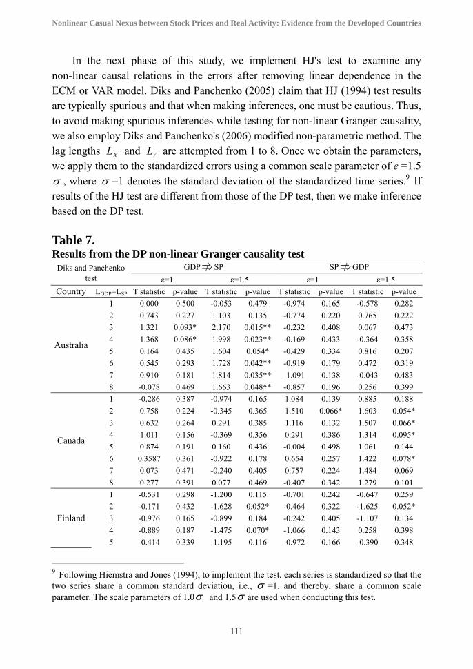
In the next phase of this study, we implement HJ's test to examine any non-linear causal relations in the errors after removing linear dependence in the ECM or VAR model. Diks and Panchenko (2005) claim that HJ (1994) test results are typically spurious and that when making inferences, one must be cautious. Thus, to avoid making spurious inferences while testing for non-linear Granger causality, we also employ Diks and Panchenko's (2006) modified non-parametric method. The lag lengths XL and YL are attempted from 1 to 8. Once we obtain the parameters, we apply them to the standardized errors using a common scale parameter of e =1.5 , where =1 denotes the standard deviation of the standardized time series.9 If results of the HJ test are different from those of the DP test, then we make inference based on the DP test. Table 7. Results from the DP non-linear Granger causality test

Diks and Panchenko test

GDP SP SP GDP

ε=1 ε=1.5 ε=1 ε=1.5

Country LGDP=LSP T statistic p-value T statistic p-value T statistic p-value T statistic p-value

Australia

1 0.000 0.500 -0.053 0.479 -0.974 0.165 -0.578 0.282

2 0.743 0.227 1.103 0.135 -0.774 0.220 0.765 0.222

3 1.321 0.093* 2.170 0.015** -0.232 0.408 0.067 0.473

4 1.368 0.086* 1.998 0.023** -0.169 0.433 -0.364 0.358

5 0.164 0.435 1.604 0.054* -0.429 0.334 0.816 0.207

6 0.545 0.293 1.728 0.042** -0.919 0.179 0.472 0.319

7 0.910 0.181 1.814 0.035** -1.091 0.138 -0.043 0.483

8 -0.078 0.469 1.663 0.048** -0.857 0.196 0.256 0.399

Canada

1 -0.286 0.387 -0.974 0.165 1.084 0.139 0.885 0.188

2 0.758 0.224 -0.345 0.365 1.510 0.066* 1.603 0.054*

3 0.632 0.264 0.291 0.385 1.116 0.132 1.507 0.066*

4 1.011 0.156 -0.369 0.356 0.291 0.386 1.314 0.095*

5 0.874 0.191 0.160 0.436 -0.004 0.498 1.061 0.144

6 0.3587 0.361 -0.922 0.178 0.654 0.257 1.422 0.078*

7 0.073 0.471 -0.240 0.405 0.757 0.224 1.484 0.069

8 0.277 0.391 0.077 0.469 -0.407 0.342 1.279 0.101

Finland

1 -0.531 0.298 -1.200 0.115 -0.701 0.242 -0.647 0.259

2 -0.171 0.432 -1.628 0.052* -0.464 0.322 -1.625 0.052*

3 -0.976 0.165 -0.899 0.184 -0.242 0.405 -1.107 0.134

4 -0.889 0.187 -1.475 0.070* -1.066 0.143 0.258 0.398

5 -0.414 0.339 -1.195 0.116 -0.972 0.166 -0.390 0.348

9 Following Hiemstra and Jones (1994), to implement the test, each series is standardized so that the two series share a common standard deviation, i.e., =1, and thereby, share a common scale parameter. The scale parameters of 1.0 and 1.5 are used when conducting this test.


112

6 0.964 0.168 -0.561 0.288 -0.948 0.172 0.287 0.387

7 0.656 0.256 0.036 0.486 -0.596 0.276 -0.734 0.232

8 NA NA -0.469 0.320 NA NA 0.370 0.356

France

1 -0.026 0.490 -0.402 0.344 0.169 0.433 -0.212 0.416

2 0.943 0.173 0.104 0.459 0.016 0.494 1.269 0.102

3 0.398 0.345 -0.311 0.378 0.329 0.371 1.791 0.037**

4 1.042 0.149 0.795 0.214 0.480 0.316 0.942 0.173

5 -0.088 0.465 0.680 0.248 0.759 0.224 1.091 0.138

6 -0.303 0.381 1.154 0.124 0.514 0.304 0.664 0.253

7 -0.789 0.215 0.920 0.179 0.557 0.289 1.076 0.141

8 0.000 0.500 0.594 0.276 0.742 0.229 0.910 0.182

Swiss

1 -1.281 0.100 -0.246 0.403 0.785 0.216 0.707 0.240

2 -0.780 0.218 -0.414 0.339 0.867 0.193 1.118 0.312

3 -1.381 0.084* -0.483 0.315 0.400 0.345 1.316 0.094*

4 -1.175 0.120 -0.178 0.429 -0.366 0.357 1.193 0.116

5 -0.373 0.355 -0.510 0.305 0.341 0.367 1.096 0.137

6 0.420 0.337 0.226 0.411 -0.502 0.308 1.146 0.126

7 0.555 0.290 0.352 0.362 0.181 0.428 1.302 0.097*

8 0.517 0.303 0.783 0.217 -0.505 0.307 1.185 0.118

UK

1 1.087 0.138 1.862 0.031** 0.122 0.451 -0.180 0.429

2 1.322 0.093* 1.511 0.065* 0.389 0.349 -0.699 0.242

3 1.305 0.096* 1.204 0.114 1.863 0.031** 0.675 0.250

4 0.951 0.171 1.039 0.149 1.868 0.031** 0.939 0.174

5 0.861 0.195 1.357 0.087* 1.548 0.061* 0.557 0.289

6 0.829 0.204 1.178 0.119 1.620 0.053** 1.334 0.090*

7 0.595 0.276 1.297 0.097* 1.429 0.077* 1.669 0.048**

8 0.200 0.421 1.289 0.099* 1.417 0.078* 1.269 0.102

USA

1 0.276 0.391 0.346 0.365 1.479 0.070* 0.713 0.283

2 0.767 0.221 0.174 0.431 -0.186 0.426 1.047 0.148

3 1.071 0.142 0.968 0.176 -0.230 0.409 1.048 0.147

4 1.154 0.124 1.404 0.080* -0.074 0.471 0.606 0.272

5 0.288 0.378 1.270 0.102 -0.011 0.496 0.385 0.350

6 0.437 0.331 1.739 0.041** 0.588 0.278 0.699 0.242

7 -0.131 0.448 0.578 0.282 0.339 0.367 0.435 0.322

8 0.790 0.215 1.158 0.123 -0.413 0.340 0.449 0.327


(2) GDP SP denotes real GDP do not Granger-cause stock prices. SP GDP denotes stock prices do not Granger-cause real GDP.

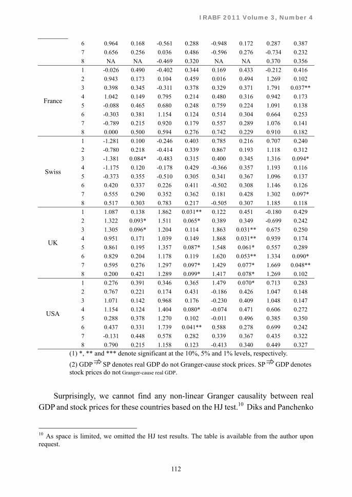
Surprisingly, we cannot find any non-linear Granger causality between real GDP and stock prices for these countries based on the HJ test.10 Diks and Panchenko

10 As space is limited, we omitted the HJ test results. The table is available from the author upon request.


113

(2006) argue that HJ’s method lacks consistency, and in its place, they propose a new test statistic for non-linear Granger causality. The DP non-linear Granger causal test results are summarized in Table 7. At the 10% significance level or better, there is a unidirectional causality running from real GDP to stock prices for Australia. Conversely, there is a unidirectional causality running from stock prices to real GDP for Canada. However, there is a bidirectional non-linear causal relation between stock prices and real GDP for the case of the Finland, Swiss, the UK and the USA at the 10% significance level or better. Therefore, the causal nexus between stock price changes and real activity is not only linear but also non-linear.

3.4 Comparisons with Previous Findings

We compare our findings with those obtained by selected researchers. Peiro (1996) investigated the relationships between stock returns, changes in production, and changes in interest rates in three European countries: France, Germany, and the United Kingdom. He found significant unidirectional causality from stock price changes to real activity only in the case of France, but not in the case of Germany and the UK. Aylward and Glen (2000) conducted an analysis using annual average data on 23 markets: the G-7 countries, plus Australia and 15 emerging market countries over a sample period from 1951–1993. Estimation results were mixed, with only 6 countries having significant coefficients on lagged stock price variables when the OLS estimation technique was used. Using the SUR estimation technique, 12 of the 23 countries in the sample were found to have significant and positive coefficients on lagged stock price variables. Mauro (2003) conducted a similar analysis on a mix of 17 developed and 8 emerging countries. Results showed positive and significant relationships for 5 out of 8 emerging markets and 10 out of 17 advanced countries. Panel estimation showed that lagged stock returns were significantly and positively associated with output growth in both advanced and emerging countries.

The different results among the studies reported could be attributed to different data samples or to different methodology. However, these studies are all based on time series linear causality tests. The short span of the data used and consequently the low statistical power of the country-by-country tests are likely to have contributed further to the conflicting results. Moreover, previous studies overlook the non-linear Granger causality while our empirical results complement these omissions. Thus, all these findings should be viewed with caution because the exclusion of non-linear property and the singular focus of many past studies on the


114

linear causality may be misleading or at best incomplete. Our analysis, by using the ARDL bounds test with good test power in small sample and incorporating non-linearity in the model, is expected to produce thus more reliable results.

4. Discussions and Concluding Remarks

This paper contributes to this literature by using multivariate cointegrated VAR methods to investigate the nexus between stock prices and real activity in seven developed countries. Two hypotheses, i.e., the stock returns-led real activity hypothesis and real activity-led stock returns hypothesis, are examined in this paper. The methodology we use has only recently been developed by Pesaran et al. (2001) and is based on the estimation of the UECM and the bounds test. The advantage of the PSS approach is that policy-makers can determine which variable is statistically endogenous and which is exogenous and distinguish between short-term and long-term Granger causality. We examine not only linear Granger causality but also non-linear Granger causality by using the nonparametric Hiemstra and Jones (1994) and Diks and Panchenko (2005, 2006) methods. This allows us to explore the links between these variables and assess the robustness of results obtained with parametric techniques.

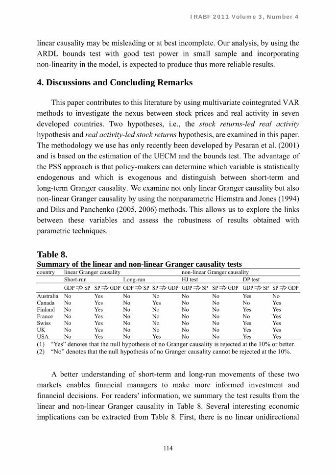
Table 8. Summary of the linear and non-linear Granger causality tests country linear Granger causality non-linear Granger causality Short-run Long-run HJ test DP test GDP SP SP GDP GDP SP SP GDP GDP SP SP GDP GDP SP SP GDP

Australia No Yes No No No No Yes No Canada No Yes No Yes No No No Yes Finland No Yes No No No No Yes Yes France No Yes No No No No No Yes Swiss No Yes No No No No Yes Yes UK No Yes No No No No Yes Yes USA No Yes No Yes No No Yes Yes (1) “Yes” denotes that the null hypothesis of no Granger causality is rejected at the 10% or better. (2) “No” denotes that the null hypothesis of no Granger causality cannot be rejected at the 10%.

A better understanding of short-term and long-run movements of these two markets enables financial managers to make more informed investment and financial decisions. For readers’ information, we summary the test results from the linear and non-linear Granger causality in Table 8. Several interesting economic implications can be extracted from Table 8. First, there is no linear unidirectional


115

causality runs from the real activity to stock price changes neither in the short-run nor in the long-run for all countries, indicating that the real activity-led stock returns (ALS) hypothesis is not favorable. The fact that real output growth does not lead stock returns implies that stock price is unpredictable by using the information contained in the real activity. The results are in favor of the efficient market hypothesis, in which asserts that past prices, volume, and other market statistics provide no information that can be used to predict future stock prices. The Granger causality test results show that the efficient market hypothesis is sustainable for these countries in the linear from.

Second, it is shown that, for all countries, the lagged stock price changes are helpful to predicting the evolution of real activity in the near future or in the short-run. In the long-run, in the case of Canada and the USA, there is a long-run caual effect runs from stock returns to real output. The results are in favor of the stock return-led real activity (SLA) hypothesis. In other words, the stock prices play the role of the leading index in forcasting the real output. So, policymakers should continuously pay attention to developments in stock market.

There are several theoretical channels to favor the SLA hypothesis. For example, optimistic expectations of future profits may cause a rise in stock prices, which is an increase in wealth, which has the likely effect of an increase in demand for consumption and investment goods, and therefore real output. The literature also identifies several channels via which movements in the stock market prices exert their influence on the real economy. The first one constitutes the consumption channel via the conventional wealth effect (Poterba, 2000). The second one relates to investment channel (Tobin, 1969), and the third one is related to the balance-sheet effect (Bernanke et al., 1998).

Third, in spite of the linear Granger causal relations, we also find evidence of the non-linear causal relations between stock returns and real outputs. It points out an important issue that we should not overlook the non-linear property in extracting the nexus between stock returns and real activity. The evidence of non-linear causality might come from the fact that consumers generally make an attempt to optimize their behavior even when faced with unpredicted changes in stock prices. For example, in stock market, the ‘bad’ news or shocks have more profound effect than the ‘good’ news. This is the well-known ‘leverage effect’. The implication of our empirical evidence is that, as opposed to focusing on changes in real activity, the authorities in these developed countries are well advised to be more mindful of changes in stock


116

prices.

Fourth, as outlined in Barro (1990) and Fama (1990), stock returns and production growth rates may also be both affected by other variables such as interest rates, inflation rates and not all changes in stock returns are caused by information on future cash flows in production. Therefore, the existence of ‘causality’ can be affected by adding more variables.11 This question deserves to be studied in the future.

Finally, this paper only examines the in-sample relations (cointegration and causality) between real output growths and stock returns using several different time series methodologies. An in-sample correlation, however, is an ex post property of the data. An alternative analysis can focus on the out-of-sample predictive power of time series models and thus provide an ex ante view of the causal relation between real output growths and stock returns. For example, Choi et al. (1999) examine the out-of-sample forecast-evaluation of the real output growths and stock returns for G7 based on procedure of Ashley et al. (1980). We leave this as an open question for interested readers.

References

Ashely, R., C. W. J. Granger and R. Schmalensee (1980), Advertising and aggregate consumption: An analysis of causality, Econometrica, 48, 1149-1167.

Aylward, A. and J. Glen (2000), Some International Evidence on Stock Prices as Leading of Economic Activity, Applied Financial Economics, 10, 1-14.

Baek, E. and W. Brock (1992), A General Test for Nonlinear Granger Causality:

11 To the authors’ best knowledge, the difference between the two-variable specification and multivariate specification when discussing ‘causality’ is on direct and indirect causal relations. When we review previous studies on the relationship between stock price and real activity, we find that a large body of studies (e.g., Gallinger, 1994; Choi et al., 1999; Hassapis and Kalyvitis, 2002a; Hassapis, 2003; Mauro, 2003; Binswanger, 2000, 2004; Henry et al., 2004; Gallegati, 2008) consider only on the two-variable specification. In other words, these studies (and our paper) emphasize on the direct causal relations between stock price and real GDP. Some authors (e.g., Cheung and Ng, 1998; Haung and Yang, 2004) think that the causal relations may well be hidden and indirect. In order to verify the indirect causality, they consider multivariate specification. This paper is intended as an investigation of the direct linear (and nonlinear) causal relations between stock price and real activity. Therefore, in line with previous researches, we focus only on a specification which consists of two variables. But, again, we cannot exclude the possibility that we may find different results when adding other variables in the system.


117

Bivariate Model, Working Paper, Iowa State University and University of Wisconsin-Madison.

Balvers, R. J., T. F. Cosimano and B. McDonlad (1990), Predicting Stock Returns in an Efficient Market, Journal of Finance, 45, 1109-1128.

Barro, R. (1990), The stock market and investment, Review of Financial Studies, 3, 115-131.

Bernanke, B. S., M. Gertler, and S. Gilchrist (1998), The Financial Accelerator in a Quantitative Business Cycle Framework. NBER Working Paper 6455.

Binswanger, M. (2000), Stock Returns and Activity: Is there Still Connection？Applied Financial Economics, 10, 379-387.

Binswanger, M. (2004), Stock Returns and Real Activity in G-7 Counties：Did the Relationship Change During the 1980s? The Quarterly Review of Economics and Finance, 44, 237-252.

Blanchard, O. (1981). Output, the Stock Market and Interest Rates, American Economic Review, 71, 132–143.

Brainard, W. and J. Tobin (1968), Pitfalls in Financial Model Building, American Economic Review, 58, 99-122.

Brock, W. A., W. Dechert, J. Scheinkman and B. LeBaron (1996), A Test for Independence Based on the Correlation Dimension, Econometric Reviews, 15, 197-235.

Canova, F and G. D. Nicolo' (1995), Stock Returns and Real Activity: A Structural Approach, European Economic Review, 39, 981-1015.

Chaudhuri I. K and S. Smilies (2004), Stock Market and Aggregate Economic Activity: Evidence from Australia, Applied Financial Economics, 14, 12-129.

Chen, P. F., C. C. Lee and S. Y. Wong (2006), Is Rate of Stock Returns a Leading Indicator of Output Growth？In the Case of Four East Asian Countries, 5th International Conference on Computational Intelligence in Economics and Finance, 1-5.

Choi, J. J., S. Hauser and K. J. Kopecky (1999), Does the Stock Market Predict Real Activity？Time Series Evidence from the G-7 Countries, Journal of Banking and Finance, 23, 1771-1792.

Dickey, D. A. and W. A. Fuller (1979), Distribution of Estimation for Autoregressive Time Series with a Unit Root, Journal of American Statistical Association, 74, 427-431.

Diks, C. and V. Panchenko (2005), A Note on the Hiemstra-Jones Test for Granger Non-Causality, studies in non-linear Dynamics and Econometrics, 9(2), article


118

4.

Diks, C. and V. Panchenko (2006), A new Statistic and Practical Guidelines for Non-Parametric Granger Causality testing, Journal of Economics Dynamics and Control, 30, 1647-1669.

Domian, D. L. and A. Louton (1997), A Threshold Autoregressive Analysis of Stock Returns and Real Economic Activity, International Review of Economics and Finance, 6, 167-197.

Elliott, G., J. T. Rothenberg and J. Stock (1996), Efficient Tests for an Autoregressive Unit Root, Econometrica, 64, 813-836.

Fama, E. F. (1981), Stock Returns, Real Activity, Inflation, and Money, American Economic Review, 71, 545-565.

Fama, E. F. (1990), Stock Returns, Expected Returns, and Real Activity, The Journal of Finance, 45, 1089-1108.

Gallegati, M. (2008), Wavelet Analysis of Stock Returns and Aggregate Economic Activity, Computational Statistics and Data Analysis, 52, 3061-3074.

Gallinger, G. W. (1994), Causality Tests of The Real Stock Return-Real Activity Hypothesis, The Journal of Financial Research, 17, 2, 271-288.

Goldsmith, R. (1969), Financial Structure and Development, New Haven, Yale University Press.

Granger, C. W. J. (1969), Investigating Causal Relations by Econometric Models and Cross-Spectral Methods, Econometrica, 37, 424-438.

Granger, C. W. J. and P. Newbold (1974), Spurious Regression in Economics, Journal of Econometrics, 12, 1045-1066.

Gregory, A. W., Bruce E. H (1996), Residual-based Tests for Cointegration in Models with Regime Shifts, Journal of Econometrics , 70, 99-126

Hassapis, C. (2003), Financial Variables and Real Activity in Canada, Canadian Journal of Economics, 36, No. 2, 422-442.

Hassapis, C. and S. Kalyvitis (2002a), Investigating the Links between Growth and Real Stock Price Changes with Empirical Evidence From the G-7 economies, Quarterly Review of Economics and Finance, 42, 543-575.

Hassapis, C. and S. Kalyvitis (2002b), On the Propagation of the Fluctuations of Stock Returns on Growth: IS the Global Effect Important? Journal of Policy Modeling, 24, 487-502.

Henry, O. T., Olekalns, N. and J. Thong, (2004), Do Stock Market Returns Predict Changes to Output? Evidence from a Nonlinear Panel Data Model, Empirical Economics, 29, 527-540.


119

Hiemstra, C. and J. D. Jones (1994), Testing for Linear and Non-linear Granger Causality in the Stock Price-volume Relation, Journal of Finance, 49, 1639-1664

Huang, B.N. and C.W Yang, (2004), Industrial Output and Stock Price Revisited: An Application of the Multivariate Indirect Causality Model, The Manchester School, 72, 3, 347-362.

Johansen, S. (1988), Statistical Analysis of Cointegration Vectors, Journal of Economic Dynamic and Control, 12, 231-254.

Johansen, S. and K. Juselius (1990), Maximum Likelihood Estimation and Inference on Cointegration with Application to the Demand for Money, Oxford Bulletin of Economics and Statistics, 52, 161-210.

Kwiatkowski, D., P. Phillips, P. Schmidt and Y. Shin (1992), Testing the Null Hypothesis of Stationary Against the Alternative of a Unit Root: How Sure Are We That Economic Time Series Have A Unit Root Journal of Econometrics, 54, 159-178.

Kwon, C. S. and T. S. Shin (1999), Cointegeration and Causality between Macroeconomic Variables and Stock Market Returns, Global Finance Journal, 10, 71-81.

Lee, B. S. (1992), Causal Relations Among Stock Returns, Interest Rates, Real Activity, and Inflation, The Journal of Finance, 47, 4, 1591-1603.

Mauro, P. (2003), Stock Returns and Output Growth in Emerging and Advanced Economies, Journal of Development Economics, 71, 129-153.

Merikas, A. G. and A. A. Merika (2006), Stock Prices Response to Real Economic Variable: The Case of Germany. Managerial Finance, 32, 5, 44-450.

Morck, R., A. Shleifer and R. W. Vishny (1990), The Stock Market and Investment: Is the Market a Sideshow? Bookings Papers on Economics Activity, 2, 157-202.

Narayan, P. K. (2005), The Saving and Investment Nexus for China: Evidence from Cointegration Tests, Applied Economics, 37, 1979-1990.

Peiro, A. (1996), Stock Price, Production and Interest Rates: Comparison of Three European Countries with the USA, Empirical Economics, 21, 221-234.

Perron, P. (1989), The Great Crash, the Oil Price Shock and the Unit Root Hypothesis, Econometrica, 57, 1361-1401.

Pesaran M. H., Shin Y. (1995), An autoregressive distributed lag modelling approach to cointegrated analysis, Discussion Paper 95-14, Department of Applied Economics, University of Cambridge.

Pesaran, M. H., Shin, Y. (1998), Structural analysis of cointegrating VARs, Journal


120

of Economic Survey, 12, 471-505.

Pesaran, M. H., Y. Shin and R. J. Smith (2001), Bounds Testing Approaches to the Analysis of Level Relationships, Journal of Applied Econometrics, 16, 289-326.

Phillips, P.C.B. (1987), Time Series Regression with a Unit Root, Econometrica, 55, 277-301.

Poterba, J. M. (2000), Stock Market Wealth and Consumption, Journal of Economic Perspectives 14 (2), 99-118.

Sarantis, C. (2001), Nonlinearities, Cyclical Behavior and Predictability in Stock Market: International Evidence, International Journal of Forecasting, 17, 459-478.

Schmidt. P. and C. B Phillips (1992), LM Test for a Unit Root in the Presence id Deterministic Trends, Oxford Bulletin of Economics and Statistic, 54, 3, 257-276.

Schwert, G. W. (1990), Stock Returns and Real Activity: A Century of Evidence, The Journal of Finance, 45, 4, 1237-1257.

Shen, C.-H. and C. C. Lee (2006), Same Financial Development Yet Different Economic Growth－Why？Journal of Money, Credit, and Banking , 38(7), 1907-1944.

Shen, C.-H. and C. P. Lin (2009), Financial Development and Economic Growth: Dynamic panel Threshold Model, Taipei Economic Inquiry, 45(2), 43-188.

Shen, C.-H., C.-C. Lee, S.-W. Chen and Z. Xie (2011), Roles Played by Financial Development in Economic Growth: Application of the Flexible Regression Model, Empirical Economics, 41(1), 103-135.

Shiller, R. (2000). Irrational Exuberance, Princeton University Press.

Siliverstovs, B. and M. H. Duong (2006), On the Role of Stock Market for Real Economic Activity: Evidence for Europe, DIW Berlin Discussion Paper, 599, 1-17.

Silvapulle, P. and M. Silvapulle (1999), Testing for Asymmetry in the Relationship between the Malaysian Business Cycle and the Stock and the Stock Market, Quarterly Journal of Business and Economics, 38, 16-25.

Stock, J. H. and M. V. Watson (1990), Business Cycle Properties of Selected U.S. Economic Time Series, 1959-1988, NBER Working Paper, No. 3376, National Bureau of Economic Research, Cambridge, Massachusetts.

Toda, H. Y. and T. Yamamoto (1995), Statistical Inference in Vector Autoregressions with Possibly Integrated Processes, Journal of Econometrics, 66, 225-250.


121

Tobin, J. (1969), A General Equilibrium Approach to Monetary Theory, Journal of Money, Credit and Banking 1, 15-29.

Toda, H. Y. and P. C. B. Phillips (1993), Vector Autoregressions and Causality, Econometrica, 58, 113-144.

Turner, P. (2006), Response surfaces for an F-test for cointegration, Applied Economics Letters, 13, 479-482.

Zivot, E. and W. K. D. Andrews (1992), Further Evidence on the Great Crash, the Oil-Price Shock, and the Unit-Root Hypothesis, Journal of Business and Economics Statistics, 10, 3, 251-270.

sample papers and commentary

Documents