sample-optimal density estimation in nearly-linear time
TRANSCRIPT

Sample-Optimal Density Estimation in Nearly-Linear Time
Jayadev Acharya∗EECS, MIT
Ilias Diakonikolas†Informatics, U. of Edinburgh
Jerry Li‡EECS, MIT
Ludwig Schmidt§EECS, MIT
June 27, 2015
Abstract
We design a new, fast algorithm for agnostically learning univariate probability distributionswhose densities are well approximated by piecewise polynomial functions. Let f be the densityfunction of an arbitrary univariate distribution, and suppose that f is OPT close in L1-distanceto an unknown piecewise polynomial function with t interval pieces and degree d. Our algorithmdraws n = O(t(d+ 1)/ε2) samples from f , runs in time O(n · poly(d)), and with probability atleast 9/10 outputs an O(t)-piecewise degree-d hypothesis h that is 4 ·OPT + ε close to f .
Our general algorithm yields (nearly) sample-optimal and nearly-linear time estimators fora wide range of structured distribution families over both continuous and discrete domains ina unified way. For most of our applications, these are the first sample-optimal and nearly-linear time estimators in the literature. As a consequence, our work resolves the sample andcomputational complexities of a broad class of inference tasks via a single “meta-algorithm”.Moreover, we experimentally demonstrate that our algorithm performs very well in practice.
Our algorithm consists of three “levels”: (i) At the top level, we employ an iterative greedyalgorithm for finding a good partition of the real line into the pieces of a piecewise polynomial.(ii) For each piece, we show that the sub-problem of finding a good polynomial fit on the currentinterval can be solved efficiently with a separation oracle method. (iii) We reduce the task offinding a separating hyperplane to a combinatorial problem and give an efficient algorithm forthis problem. Combining these three procedures gives a density estimation algorithm with theclaimed guarantees.
∗Supported by a grant from the MIT-Shell Energy Initiative.†Supported by a Marie Curie CIG, EPSRC grant EP/L021749/1 and a SICSA grant.‡Supported by NSF grant CCF-1217921 and DOE grant DE-SC0008923.§Supported by MADALGO and a grant from the MIT-Shell Energy Initiative.

Contents
1 Introduction 11.1 Our results and techniques . . . . . . . . . . . . . . . . . . . . . . . . . . . . . . . . . 21.2 Related work . . . . . . . . . . . . . . . . . . . . . . . . . . . . . . . . . . . . . . . . 6
2 Preliminaries 7
3 Paper outline 8
4 Iterative merging algorithm 104.1 The histogram merging algorithm . . . . . . . . . . . . . . . . . . . . . . . . . . . . . 104.2 The general merging algorithm . . . . . . . . . . . . . . . . . . . . . . . . . . . . . . 174.3 Putting everything together . . . . . . . . . . . . . . . . . . . . . . . . . . . . . . . . 19
5 A fast Ak-projection oracle for polynomials 205.1 The set of feasible polynomials . . . . . . . . . . . . . . . . . . . . . . . . . . . . . . 215.2 Separation oracles and approximately feasible polynomials . . . . . . . . . . . . . . . 235.3 Bounds on the radii of enclosing and enclosed balls . . . . . . . . . . . . . . . . . . . 245.4 Finding the best polynomial . . . . . . . . . . . . . . . . . . . . . . . . . . . . . . . . 26
6 The separation oracle and the Ak-computation oracle 296.1 Overview of ApproxSepOracle . . . . . . . . . . . . . . . . . . . . . . . . . . . . . 296.2 Testing non-negativity and boundedness . . . . . . . . . . . . . . . . . . . . . . . . . 306.3 An Ak-computation oracle . . . . . . . . . . . . . . . . . . . . . . . . . . . . . . . . . 31
7 Applications 407.1 Mixture of log-concave distributions . . . . . . . . . . . . . . . . . . . . . . . . . . . 407.2 Mixture of Gaussians . . . . . . . . . . . . . . . . . . . . . . . . . . . . . . . . . . . . 417.3 Densities in Besov spaces . . . . . . . . . . . . . . . . . . . . . . . . . . . . . . . . . 417.4 Mixtures of t-monotone distributions . . . . . . . . . . . . . . . . . . . . . . . . . . . 427.5 Mixtures of discrete distributions . . . . . . . . . . . . . . . . . . . . . . . . . . . . . 43
8 Experimental Evaluation 438.1 Histogram hypotheses . . . . . . . . . . . . . . . . . . . . . . . . . . . . . . . . . . . 448.2 Piecewise linear hypotheses . . . . . . . . . . . . . . . . . . . . . . . . . . . . . . . . 45
A Analysis of the General Merging Algorithm: Proof of Theorem 17 53
B Additional Omitted Proofs 57B.1 Proof of Fact 26 . . . . . . . . . . . . . . . . . . . . . . . . . . . . . . . . . . . . . . . 57B.2 Proof of Lemma 34 . . . . . . . . . . . . . . . . . . . . . . . . . . . . . . . . . . . . . 59
C Learning discrete piecewise polynomials 61C.1 Problem statement in the discrete setting . . . . . . . . . . . . . . . . . . . . . . . . 62C.2 The algorithm in the discrete setting . . . . . . . . . . . . . . . . . . . . . . . . . . . 62
1 Introduction
Estimating an unknown probability density function based on observed data is a classical problemin statistics that has been studied since the late nineteenth century, starting with the pioneeringwork of Karl Pearson [Pea95]. Distribution estimation has become a paradigmatic and fundamentalunsupervised learning problem with a rich history and extensive literature (see e.g., [BBBB72,DG85, Sil86, Sco92, DL01]). A number of general methods for estimating distributions have beenproposed in the mathematical statistics literature, including histograms, kernels, nearest neighborestimators, orthogonal series estimators, maximum likelihood, and more. We refer the reader to[Ize91] for a survey of these techniques. During the past few decades, there has been a large body ofwork on this topic in computer science with a focus on computational efficiency [KMR+94, FM99,FOS05, BS10, KMV10, MV10, KSV08, VW02, DDS12a, DDS12b, DDO+13, CDSS14a].
Suppose that we are given a number of samples from an unknown distribution that belongs to(or is well-approximated by) a given family of distributions C, e.g., it is a mixture of a small numberof Gaussians. Our goal is to estimate the unknown distribution in a precise, well-defined way. Inthis work, we focus on the problem of density estimation (non-proper learning), where the goal is tooutput an approximation of the unknown density without any constraints on its representation. Thatis, the output hypothesis is not necessarily a member of the family C. The “gold standard” in thissetting is to design learning algorithms that are both statistically and computationally efficient. Morespecifically, the ultimate goal is to obtain estimators whose sample size is information–theoreticallyoptimal, and whose running time is (nearly) linear in their sample size. An important additionalrequirement is that our learning algorithms are agnostic or robust under model misspecification,i.e., they succeed even if the target distribution does not belong to the given family C but is merelywell-approximated by a distribution in C.
We study the problem of density estimation for univariate distributions, i.e., distributions with adensity f : Ω→ R+, where the sample space Ω is a subset of the real line. While density estimationfor families of univariate distributions has been studied for several decades, both the sample andtime complexity were not yet well understood before this work, even for surprisingly simple classes ofdistributions, such as mixtures of Binomials and mixtures of Gaussians. Our main result is a generallearning algorithm that can be used to estimate a wide variety of structured distribution families.For each such family, our general algorithm simultaneously satisfies all three of the aforementionedcriteria, i.e., it is agnostic, (nearly) sample optimal, and runs in nearly-linear time.
Our algorithm is based on learning a piecewise polynomial function that approximates theunknown density. The approach of using piecewise polynomial approximation has been employedin this context before — our main contribution is to improve the computational complexity of thismethod and to make it nearly-optimal for a wide range of distribution families. The key idea of usingpiecewise polynomials for learning is that the existence of good piecewise polynomial approximationsfor a family C of distributions can be leveraged for the design of efficient learning algorithms for thefamily C. The main algorithmic ingredient that makes this method possible is an efficient procedurefor agnostically learning piecewise polynomial density functions. In prior work, Chan, Diakonikolas,Servedio, and Sun [CDSS14a] obtained a nearly-sample optimal and polynomial time algorithm forthis learning problem. Unfortunately, however, the polynomial exponent in their running time isquite high, which makes their algorithm prohibitively slow for most applications.
In this paper, we design a new, fast algorithm for agnostically learning piecewise polynomialdistributions, which in turn yields sample-optimal and nearly-linear time estimators for a wide rangeof structured distribution families over both continuous and discrete domains. For most of our
1

applications, these are the first sample-optimal and nearly-linear time estimators in the literature.As a consequence, our work resolves the sample and computational complexity of a broad class ofinference tasks via a single “meta-algorithm”. Moreover, we experimentally demonstrate that ouralgorithm performs very well in practice. We stress that a significant number of new algorithmicand technical ideas are needed for our main result, as we explain next.
1.1 Our results and techniques
In this section, we describe our results in detail, compare them to prior work, and give an overviewof our new algorithmic ideas.
Preliminaries. We consider univariate probability density functions (pdf’s) defined over a knownfinite interval I ⊆ R. (We remark that this assumption is without loss of generality and our resultseasily apply to densities defined over the entire real line.)
We focus on a standard notion of learning an unknown probability distribution from sam-ples [KMR+94], which is a natural analogue of Valiant’s well-known PAC model for learning Booleanfunctions [Val84] to the unsupervised setting of learning an unknown probability distribution. (Weremark that our definition is essentially equivalent to the notion of the L1 minimax rate of conver-gence in statistics [DL01].) A distribution learning problem is defined by a class C of probabilitydistributions over a domain Ω. Given ε > 0 and sample access to an unknown distribution with den-sity f , the goal of an agnostic learning algorithm for C is to compute a hypothesis h such that, withprobability at least 9/10, it holds ‖h− f‖1 ≤ C ·OPTC(f) + ε, where OPTC(f) := infq∈C ‖q − f‖1,i.e., OPTC(f) is the L1-distance between the unknown density f and the closest distribution to itin C, and C ≥ 1 is a universal constant.
We say that a function f over an interval I is a t-piecewise degree-d polynomial if there is apartition of I into t disjoint intervals I1, . . . , It such that f(x) = fj(x) for all x ∈ Ij , where each off1, . . . , ft is a polynomial of degree at most d. Let Pt,d(I) denote the class of all t-piecewise degree-dpolynomials over the interval I.
Our Results. Our main algorithmic result is the following:
Theorem 1 (Main). Let f : I → R+ be the density of an unknown distribution over I, where Iis either an interval or the discrete set [N ]. There is an algorithm with the following performanceguarantee: Given parameters t, d ∈ Z+, an error tolerance ε > 0, and any γ > 0, the algorithm drawsn = Oγ(t(d + 1)/ε2) samples from the unknown distribution, runs in time O(n · poly(d + 1)), andwith probability at least 9/10 outputs an O(t)-piecewise degree-d hypothesis h such that ‖f − h‖1 ≤(3 + γ)OPTt,d(f) + ε, where OPTt,d(f) := infr∈Pt,d(I) ‖f − r‖1 is the error of the best t-piecewisedegree-d approximation to f .
In prior work, [CDSS14a] gave a learning algorithm for this problem that uses O(t(d + 1)/ε2)samples and runs in poly(t, d + 1, 1/ε) time. We stress that the algorithm of [CDSS14a] is pro-hibitively slow. In particular, the running time of their approach is Ω(t3 · (d3.5/ε3.5 + d6.5/ε2.5)),which renders their result more of a “proof of principle” than a computationally efficient algorithm.
This prompts the following question: Is such a high running time necessary to achieve thislevel of sample efficiency? Ideally, one would like a sample-optimal algorithm with a low-orderpolynomial running time (ideally, linear).
Our main result shows that this is indeed possible in a very strong sense. The running time of ouralgorithm is linear in t/ε2 (up to a log(1/ε) factor), which is essentially the best possible; the polyno-mial dependence on d is O(d3+ω), where ω is the matrix multiplication exponent. This substantially
2

improved running time is of critical importance for the applications of Theorem 1. Moreover, thesample complexity of our algorithm removes the extraneous logarithmic factors present in the sam-ple complexity of [CDSS14a] and matches the information-theoretic lower bound up to a constantfactor. As we explain below, Theorem 1 leads to (nearly) sample-optimal and nearly-linear timeestimators for a wide range of natural and well-studied families. For most of these applications,ours is the first estimator with simultaneously nearly optimal sample and time complexity.
Our new algorithm is clean and modular. As a result, Theorem 1 also applies to discretedistributions over an ordered domain (e.g., [N ]). The approach of [CDSS14a] does not extend topolynomial approximation over discrete domains, and designing such an algorithm was left as anopen problem in their work. As a consequence, we obtain several new applications to learningmixtures of discrete distributions. In particular, we obtain the first nearly sample optimal andnearly-linear time estimators for mixtures of Binomial and Poisson distributions. To the best ofour knowledge, no polynomial time algorithm with nearly optimal sample complexity was knownfor these basic learning problems prior to this work.
Applications. We now explain how to use Theorem 1 in order to agnostically learn structureddistribution families. Given a class C that we want to learn, we proceed as follows: (i) Provethat any distribution in C is ε/2-close in L1-distance to a t-piecewise degree-d polynomial, forappropriate values of t and d. (ii) Use Theorem 1 for these values of t and d to agnostically learnthe target distribution up to error ε/2. Note that t and d will depend on the desired error ε and theunderlying class C. We emphasize that there are many combinations of t and d that guarantee anε/2-approximation of C in Step (i). To minimize the sample complexity of our learning algorithmin Step (ii), we would like to determine the values of t and d that minimize the product t(d + 1).This is, of course, an approximation theory problem that depends on the structure of the family C.
For example, if C is the family of log-concave distributions, the optimal t-histogram approxima-tion with accuracy ε requires Θ(1/ε) intervals. This leads to an algorithm with sample complexityΘ(1/ε3). On the other hand, it can be shown that any log-concave distribution has a piecewise linearε-approximation with Θ(1/ε1/2) intervals [CDSS14a, DK15], which yields an algorithm with samplecomplexity Θ(1/ε5/2). Perhaps surprisingly, this sample bound cannot be improved using higherdegree piecewise polynomials; one can show an information-theoretic lower bound of Ω(1/ε5/2) forlearning log-concave densities [DL01]. Hence, Theorem 1 gives a sample-optimal and nearly-lineartime agnostic learning algorithm for this fundamental problem. We remark that piecewise polyno-mial approximations are “closed” under taking mixtures. As a corollary, Theorem 1 also yields anO(k/ε5/2) sample and nearly-linear time algorithm for learning an arbitrary mixture of k log-concavedistributions. Again, there exists a matching information-theoretic lower bound of Ω(k/ε5/2).
As a second example, let C be the class of mixtures of k Gaussians in one dimension. Itis not difficult to show that learning such a mixture of Gaussians up to L1-distance ε requiresΩ(k/ε2) samples. By approximating the corresponding probability density functions with piecewisepolynomials of degree O(log(1/ε)), we obtain an agnostic learning algorithm for this class that usesn = O(k/ε2) samples and runs in time O(n). Similar bounds can be obtained for several othernatural parametric mixture families.
Note that for a wide range of structured families,1 the optimal choice of the degree d (i.e., thechoice minimizing t(d+1) among all ε/2-approximations) will be at most poly-logarithmic in 1/ε. For
1This includes all structured families considered in [CDSS14a] and several previously-studied distributions notcovered by [CDSS14a].
3

several classes (such as unimodal, monotone hazard rate, and log-concave distributions), the degreed is even a constant. As a consequence, Theorem 1 yields (nearly) sample optimal and nearly-lineartime estimators for all these families in a unified way. In particular, we obtain sample optimal (ornearly sample optimal) and nearly-linear time estimators for a wide range of structured distributionfamilies, including arbitrary mixtures of natural distributions such as multi-modal, concave, convex,log-concave, monotone hazard rate, Gaussian, Poisson, Binomial, functions in Besov spaces, andothers.
See Table 1 for a summary of these applications. For each distribution family in the table, weprovide a comparison to the best previous result. Note that we do not aim to exhaustively cover allpossible applications of Theorem 1, but rather to give some selected applications that are indicativeof the generality and power of our method.
Moreover, our non-proper learning algorithm is also useful for proper learning. Indeed, Theo-rem 1 has recently been used [LS15] as a crucial component to obtain the fastest known agnosticalgorithm for properly learning a mixture of univariate Gaussian distributions. Note that non-properlearning and proper learning for a family C are equivalent in terms of sample complexity: given any(non-proper) hypothesis, we can perform a brute-force search to find its closest approximation inthe class C. The challenging part is to perform this computation efficiently. Roughly speaking, givena piecewise polynomial hypothesis, [LS15] design an efficient algorithm to find the closest mixtureof k Gaussians.
Our Techniques. We now provide a brief overview of our new algorithm and techniques in parallelwith a comparison to the previous algorithm of [CDSS14a]. We require the following definition.For any k ≥ 1 and an interval I ⊆ R, define the Ak-norm of a function g : I → R to be
‖g‖Akdef= sup
I1,...,Ik
k∑i=1
|g(Ii)| ,
where the supremum is over all sets of k disjoint intervals I1, . . . , Ik in I, and g(J)def=∫J g(x) dx for
any measurable set J ⊆ I. Our main probabilistic tool is the following well-known version of theVC inequality:
Theorem 2 (VC Inequality [VC71, DL01]). Let f : I → R+ be an arbitrary pdf over I, and let fbe the empirical pdf obtained after taking n i.i.d. samples from f . Then
E[‖f − f‖Ak ] ≤ O
(√k
n
).
Given this theorem, it is not difficult to show that the following two-step procedure is an agnosticlearning algorithm for Pt,d:
(1) Draw a set of n = Θ(t(d+ 1)/ε2) samples from f ;
(2) Output the piecewise-polynomial hypothesis h ∈ Pt,d that minimizes the quantity ‖h− f‖Akup to an additive error of O(ε), where k = O(t(d+ 1)).
We remark that the optimization problem in Step (2) is non-convex. However, it has sufficientstructure so that it can be solved in polynomial time. Intuitively, an algorithm for Step (2) involvestwo main ingredients:
4

Class of distributions Samplecomplexity
Timecomplexity Reference Optimality
t-histograms O( tε2
) O( tε2
) [CDSS14b]
O( tε2
) O( tε2
log(1/ε)) Theorem 10 SO, T OSt-piecewise
degree-d polynomialsO( t·d
ε2) O
(t3 · (d3.5
ε3.5+ d6.5
ε2.5))
[CDSS14a]
O( t·dε2
) O( t·dω+3
ε2) Theorem 1 NSO
k-mixture of log-concave O( kε5/2
) O(k3
ε5) [CDSS14a]
O( kε5/2
) O( kε5/2
) Theorem 42 SO, NT Ok-mixture of Gaussians O( k
ε2) O( k3
ε3.5) [CDSS14a]
O(k log(1/ε)ε2
) O( kε2
) Theorem 43 NSO, NT OBesov space Bα
q (Lp([0, 1])) Oα
(log2(1/ε)
ε2+1/α
)Oα
(1
ε6+3/α
)[WN07]
Oα
(1
ε2+1/α
)Oα
(1
ε2+1/α
)Theorem 44 SO, NT O
k-mixture of t-monotone O( t·kε2+1/t ) O( k3
ε3/t· ( t3.5ε3.5
+ t6.5
ε2.5)) [CDSS14a]
O( t·kε2+1/t ) O(k·t
2+ω
ε2+1/t ) Theorem 45 SO,NT Ofor t = 1, 2
k-mixture of t-modal O( t·k log(N)ε3
) O( t·k log(N)ε3
) [CDSS14b]
O( t·k log(N)ε3
) O( t·k log(N)ε3
log(1/ε)) Theorem 46 SO, T OSk-mixture of MHR O(k log(N/ε)
ε3)) O(k log(N/ε)
ε3)) [CDSS14b]
O(k log(N/ε)ε3
) O(k log(N/ε)ε3
log(1/ε)) Theorem 47 SO, T OSk-mixture of
Binomial, Poisson O( kε3
) O( kε3
) [CDSS14b]
O(k log(1/ε)ε2
) O( kε2
) Theorem 48 NSO, NT O
SO : Sample complexity is optimal up to a constant factor.NSO : Sample complexity is optimal up to a poly-logarithmic factor.T OS : Time complexity is optimal (up to sorting the samples).NT O : Time complexity is optimal up to a poly-logarithmic factor.
Table 1: A list of applications to agnostically learning specific families of distributions. For eachclass, the first row is the best known previous result and the second row is our result. Note that formost of the examples, our algorithm runs in time that is nearly-linear in the information-theoreticallyoptimal sample complexity. The last three classes are over discrete sets, and N denotes the size ofthe support.
(2.1) An efficient procedure to find a good set t intervals.
(2.2) An efficient procedure to agnostically learn a degree-d polynomial in a given sub-interval ofthe domain.
We remark that the procedure for (2.1) will use the procedure for (2.2) multiple times as a subroutine.[CDSS14a] solve an appropriately relaxed version of Step (2) by a combination of linear pro-
5

gramming and dynamic programming. Roughly speaking, they formulate a polynomial size linearprogram to agnostically learn a degree-d polynomial in a given interval, and use a dynamic pro-gram in order to discover the correct t intervals. It should be emphasized that the algorithmof [CDSS14a] is theoretically efficient (polynomial time), but prohibitively slow for real applica-tions with large data sets. In particular, the linear program of [CDSS14a] has Ω(d/ε) variables andΩ(d2/ε2 + d5/ε) constraints. Hence, the running time of their algorithm using the fastest knownLP solver for their instance [LS14] is at least Ω(d3.5/ε3.5 + d6.5/ε2.5). Moreover, the dynamic pro-gram to implement (2) has running time at least Ω(t3). This leads to an overall running time ofΩ(t3 · (d3.5/ε3.5 + d6.5/ε2.5)
), which quickly becomes unrealistic even for modest values of ε, t, and
d.We now provide a sketch of our new algorithm. At a high-level, we implement procedure (2.1)
above using an iterative greedy algorithm. Our algorithm circumvents the need for a dynamicprogramming approach as follows: The main idea is to iteratively merge pairs of intervals by callingan oracle for procedure (2.2) in every step until the number of intervals becomes O(t). Our iterativealgorithm and its subtle analysis are directly inspired by the VC inequality. Roughly speaking, ineach iteration the algorithm estimates the contribution to an appropriate notion of error when twoconsecutive intervals are merged, and it merges pairs of intervals with small error. This procedureensures that the number of intervals in our partition decreases geometrically with the number ofiterations.
Our algorithm for procedure (2.2) is based on convex programming and runs in time poly(d +1)/ε2 (note that the dependence on ε is optimal). To achieve this significant running time improve-ment, we use a novel approach that is quite different from that of [CDSS14a]. Roughly speaking,we are able to exploit the problem structure inherent in the Ak optimization problem in order toseparate the problem dimension d from the problem dimension 1/ε, and only solve a convex programof dimension d (as opposed to dimension poly(d/ε) in [CDSS14a]). More specifically, we considerthe convex set of non-negative polynomials with Ad+1 distance at most τ from the empirical distri-bution. While this set is defined through a large number of constraints, we show that it is possibleto design a separation oracle that runs in time nearly linear in both the number of samples and thedegree d. Combined with tools from convex optimization such as the Ellipsoid method or Vaidya’salgorithm, this gives an efficient algorithm for procedure (2.2).
1.2 Related work
There is a long history of research in statistics on estimating structured families of distributions.For distributions over continuous domains, a very natural type of structure to consider is some sortof “shape constraint” on the probability density function (pdf) defining the distribution. Statisticalresearch in this area started in the 1950’s, and the reader is referred to the book [BBBB72] for a sum-mary of the early work. Most of the literature in shape-constrained density estimation has focusedon one-dimensional distributions, with a few exceptions during the past decade. Various structuralrestrictions have been studied over the years, starting from monotonicity, unimodality, convexity,and concavity [Gre56, Bru58, Rao69, Weg70, HP76, Gro85, Bir87a, Bir87b, Fou97, CT04, JW09],and more recently focusing on structural restrictions such as log-concavity and k-monotonicity[BW07, DR09, BRW09, GW09, BW10, KM10, Wal09, DW13, CS13, KS14, BD14, HW15]. Thereader is referred to [GJ14] for a recent book on the subject. Mixtures of structured distributionshave received much attention in statistics [Lin95, RW84, TSM85, LB99] and, more recently, intheoretical computer science [Das99, DS00, AK01, VW02, FOS05, AM05, MV10].
6

The most common method used in statistics to address shape-constrained inference problems isthe Maximum Likelihood Estimator (MLE) and its variants. While the MLE is very popular andquite natural, we note that it is not agnostic, and it may in general require solving an intractableoptimization problem (e.g., for the case of mixture models.)
Piecewise polynomials (splines) have been extensively used as tools for inference tasks, includingdensity estimation, see, e.g., [WW83, WN07, Sto94, SHKT97]. We remark that splines in thestatistics literature have been used in the context of the MLE, which is very different than ourapproach. Moreover, the degree of the splines used is typically bounded by a small constant andthe underlying algorithms are heuristic in most cases. A related line of work in mathematicalstatistics [KP92, DJKP95, KPT96, DJKP96, DJ98] uses non-linear estimators based on wavelettechniques to learn continuous distributions whose densities satisfy various smoothness constraints,such as Triebel and Besov-type smoothness. We remark that the focus of these works is usually onthe statistical efficiency of the proposed estimators.
For the problem of learning piecewise constant distributions with t unknown interval pieces,[CDSS14b] recently gave an n = O(t/ε2) sample and O(n) time algorithm. However, their approachdoes not seem to generalize to higher degrees. Moreover, recall that Theorem 1 removes all loga-rithmic factors from the sample complexity. Furthermore, our algorithm runs in time proportionalto the time required to sort the samples, while their algorithm has additional logarithmic factors inthe running time (see Table 1).
Our iterative merging idea is quite robust: together with Hegde, the authors of the currentpaper have shown that an analogous approach yields sample optimal and efficient algorithms foragnostically learning discrete distributions with piecewise constant functions under the `2-distancemetric [ADH+15]. We emphasize that learning under the `2-distance is easier than under the L1-distance, and that the analysis of [ADH+15] is significantly simpler than the analysis in the currentpaper. Moreover, the algorithmic subroutine of finding a good polynomial fit on a fixed intervalrequired by the `2 algorithm is substantially simpler than the subroutine we require here. Indeed, inour case, the associated optimization problem has exponentially many linear constraints, and thuscannot be fully described, even in polynomial time.
Paper Structure. After some preliminaries in Section 2, we give an outline of our algorithmin Section 3. Sections 4 – 6 contain the various components of our algorithm. Section 7 gives adetailed description of our applications to learning structured distribution families, and we concludein Section 8 with our experimental evaluation.
2 Preliminaries
We consider univariate probability density functions (pdf’s) defined over a known finite intervalI ⊆ R. For an interval J ⊆ I and a positive integer k, we will denote by IkJ the family of all sets of kdisjoint intervals I1, . . . , Ik where each Ii ⊆ J . For a measurable function g : I → R and a measurableset S, let g(S)
def=∫S g. The L1-norm of g over a subinterval J ⊆ I is defined as ‖g‖1,J
def=∫J |g(x)|dx.
More generally, for any set of disjoint intervals J ∈ IkI , we define ‖g‖1,J =∑
J∈J ‖g‖1,J .We now define a norm which induces a corresponding distance metric that will be crucial for
this paper:
Definition 3 (Ak-norm). Let k be a positive integer and let g : I → R be measurable. For any
7

subinterval J ⊆ I, the Ak-norm of g on J is defined as
‖g‖Ak,Jdef= supI∈IkJ
∑M∈I|g(M)| .
When J = I, we omit the second subscript and simply write ‖g‖Ak .More generally, for any set of disjoint intervals J = J1, . . . , J` where each Ji ⊆ I, we define
‖g‖Ak,J = supI
∑J∈I|g(J)|
where the supremum is taken over all I ∈ IkJ such that for all J ∈ I there is a Ji ∈ J with J ⊆ Ji.
We note that the definition of the Ak-norm in this work is slightly different than that in [DL01,CDSS14a] but is easily seen to be essentially equivalent. The VC inequality (Theorem 2) along withuniform convergence bounds (see, e.g., Theorem 2.2. in [CDSS13] or p. 17 in [DL01]), yields thefollowing:
Corollary 4. Fix 0 < ε and δ < 1. Let f : I → R+ be an arbitrary pdf over I, and let f bethe empirical pdf obtained after taking n = Θ((k + log 1/δ)/ε2) i.i.d. samples from f . Then withprobability at least 1− δ,
‖f − f‖Ak ≤ ε .
Definition 5. Let g : I → R. We say that g has at most k sign changes if there exists a partitionof I into intervals I1, . . . , Ik+1 such that for all i ∈ [k+ 1] either g(x) ≥ 0 for all x ∈ Ii or g(x) ≤ 0for all x ∈ Ii.
We will need the following elementary facts about the Ak-norm.
Fact 6. Let J ⊆ I be an arbitrary interval or a finite set of intervals. Let g : I → R be a measurablefunction.
(a) If g has at most k − 1 sign changes in J , then ‖g‖1,J = ‖g‖Ak,J .
(b) For all k ≥ 1, we have ‖g‖Ak,J ≤ ‖g‖1,J .
(c) Let α be a positive integer. Then, ‖g‖Aα·k,I ≤ α · ‖g‖Ak,I .
(d) Let f : I → R+ be a pdf over I, and let J1, . . . ,J` be finite sets of disjoint subintervals ofI, such that for all i, i′ and for all I ∈ Ji and I ′ ∈ Ji′, I and I ′ are disjoint. Then, for allpositive integers m1, . . . ,m`,
∑`i=1‖f‖Ami ,Ji ≤ ‖f‖AM , where M =
∑`i=1mi.
3 Paper outline
In this section, we give a high-level description of our algorithm for learning t-piecewise degree-dpolyonomials. Our algorithm can be divided into three layers.
8

Level 1: General merging (Section 4). At the top level, we design an iterative mergingalgorithm for finding the closest piecewise polynomial approximation to the unknown target density.Our merging algorithm applies more generally to broad classes of piecewise hypotheses. Let D bea class of hypotheses satisfying the following: (i) The number of intersections between any twohypotheses in D is bounded. (ii) Given an interval J and an empirical distribution f , we canefficiently find the best fit to f from functions in D with respect to the Ak-distance. (iii) We canefficiently compute the Ak-distance between the empirical distribution and any hypothesis in D.Under these assumptions, our merging algorithm agnostically learns piecewise hypotheses whereeach piece is in the class D.
In Section 4.1, we start by presenting our merging algorithm for the case of piecewise constanthypotheses. This interesting special case captures many of the ideas of the general case. In Section4.2, we proceed to present our general merging algorithm that applies all classes of distributionssatisfying properties (i)-(iii).
When we adapt the general merging algorithm to a new class of piecewise hypotheses, the mainalgorithmic challenge is constructing a procedure for property (ii). More formally, we require aprocedure with the following guarantee.
Definition 7. Fix η > 0. An algorithm Op(f , J, η) is an η-approximate Ak-projection oracle forD if it takes as input an interval J and f , and returns a hypothesis h ∈ D such that
‖h− f‖Ak ≤ infh′∈D‖h′ − f‖Ak,J + η .
One of our main contributions is an efficient Ak-projection oracle for the class of degree-dpolynomials, which we describe next.
Level 2: Ak-projection for polynomials (Section 5). Our Ak-projection oracle computes thecoefficients c ∈ Rd+1 of a degree-d polynomial pc that approximately minimizes the Ak-distanceto the empirical distribution f in the given interval J . Moreover, our oracle ensures that pc isnon-negative on J .
At a high-level, we formulate the Ak-projection as a convex optimization problem. A key insightis that we can construct an efficient, approximate separation oracle for the set of polynomials thathave an Ak-distance of at most τ to the empirical distribution f . Combining this separation oraclewith existing convex optimization algorithms allows us to solve the feasibility problem of checkingwhether we can achieve a given Ak-distance τ . We then convert the feasibility problem to theoptimization variant via a binary search over τ .
Note that the set of non-negative polynomials is a spectrahedron (the feasible set of a semidefiniteprogram). After restricting the set of coefficients to non-negative polynomials, we can simplify thedefinition of the Ak-distance: it suffices to consider sets of intervals with endpoints at the locationsof samples. Hence, we can replace the supremum in the definition of the Ak-distance by a maximumover a finite set, which shows that the set of polynomials that are both non-negative and τ -closeto f in Ak-distance is also a spectrahedron. This suggests that the Ak-projection problem couldbe solved by a black-box application of an SDP solver. However, this would lead to a running timethat is exponential in k because there are more than
(s
2k
)possible sets of intervals, where s is the
number of sample points in the current interval J .2
2While the authors of [CDSS14a] introduce an encoding of the Ak-constraint with fewer linear inequalities, their
9

Instead of using black-box SDP or LP solvers, we construct an algorithm that exploits additionalstructure in the Ak-projection problem. Most importantly, our algorithm separates the dimensionof the desired degree-d polynomial from the number of samples (or equivalently, the error parameterε). This allows us to achieve a running time that is nearly-linear for a wide range of distributions.Interestingly, we can solve our SDP significantly faster than the LP which has been proposed in[CDSS14a] for the same problem. We achieve this by combining Vaidya’s cutting plane method[Vai96] with an efficient separation oracle that leverages the structure of the Ak-distance. Thisseparation oracle is the third level of our algorithm, which we describe next.
Level 3: Ak-separation oracle for polynomials (Section 6). Our separation oracle efficientlytests two properties for a given polynomial pc with coefficients c ∈ Rd+1: (i) Is the polynomialpc non-negative on the given interval J? (ii) Is the Ak-distance between pc and the empiricaldistribution f at most τ? We implement Test (i) by using known algorithms for finding roots ofreal polynomials efficiently [Pan01]. Note, however, that root-finding algorithms cannot be exactfor degrees larger than 4. Hence, we can only approximately Test (i), which necessarily leads toan approximate separation oracle. Nevertheless, we show that such an approximate oracle is stillsufficient for solving the convex program outlined above.
At a high level, our algorithm proceeds as follows. We first verify that our current candidatepolynomial pc is “nearly” non-negative at every point in J . Assuming that pc passes this test,we then focus on the problem of computing the Ak-distance between pc and f . We reduce thisproblem to a discrete variant by showing that the endpoints of intervals jointly maximizing theAk-distance are guaranteed to coincide with sample points of the empirical distribution (assumingpc is nearly non-negative on the current interval). Our discrete variant of this problem is relatedto a previously studied question in computational biology, namely finding maximum-scoring DNAsegment sets [Csu04]. We exploit this connection and give a combinatorial algorithm for this discretevariant that runs in time nearly-linear in the number of sample points in J and the degree d. Oncewe have found a set of intervals maximizing the Ak-distance, we can convert it to a separatinghyperplane for the polynomial coefficients c and the set of non-negative polynomials with Ak-distance at most τ to f .
Combining these ingredients yields our general algorithm with the performance guarantees statedin Theorem 1.
4 Iterative merging algorithm
In this section, we describe and analyze our iterative merging algorithm. We start with the case ofhistograms and then provide the generalization to piecewise polynomials.
4.1 The histogram merging algorithm
A t-histogram is a function h : I → R that is piecewise constant with at most t interval pieces,i.e., there is a partition of I into intervals I1, . . . , It′ with t′ ≤ t such that h is constant on eachIi. Given sample access to an arbitrary pdf f over I and a positive integer t, we would like to
approach increases the number of variables in the optimization problem to depend polynomially on 1/ε, which leadsto an Ω(poly(d+ 1)/ε3.5) running time. In contrast, our approach achieves a nearly optimal dependence on ε that isO(poly(d+ 1)/ε2).
10

efficiently compute a good t-histogram approximation to f . Namely, if Ht = Ht(I) denotes the setof t-histogram probability density functions over I and OPTt = infg∈Ht ‖g − f‖1, our goal is tooutput an O(t)-histogram h : I → R that satisfies ‖h−f‖1 ≤ C ·OPTt+O(ε) with high probabilityover the samples, where C is a universal constant.
The following notion of flattening a function over an interval will be crucial for our algorithm:
Definition 8. For a function g : I → R and an interval J = [u, v] ⊆ I, we define the flattening ofg over J , denoted gJ , to be the constant function defined on J as
gJ(x)def=
g(J)
v − ufor all x ∈ J.
For a set I of disjoint intervals in I, we define the flattening of g over I to be the function gI on∪J∈IJ which for each J ∈ I satisfies gI(x) = gJ(x) for all x ∈ J .
We start by providing an intuitive explanation of our algorithm followed by a proof of correctness.The algorithm draws n = Θ((t + log 1/δ)/ε2) samples x1 ≤ x2 ≤ . . . ≤ xn from f . We start withthe following partition of I = [a, b]:
I0 = [a, x1), [x1, x1], (x1, x2), [x2, x2], . . . , (xn−1, xn), [xn, xn], (xn, b]. (1)
This is the partition where each interval is either a single sample point or the interval between twoconsecutive samples. Starting from this partition, our algorithm greedily merges pairs of consecutiveintervals in a sequence of iterations. When deciding which interval pairs to merge, the followingnotion of approximation error will be crucial:
Definition 9. For a function g : I → R and an interval J ⊆ I, define e(g, J) = ‖g − gJ‖A1,J. We
call this quantity the A1-error of g on J .
In the j-th iteration, given the current interval partition Ij , we greedily merge pairs of consecu-tive intervals to form the new partition Ij+1. Let sj be the number of intervals in Ij . In particular,given Ij = I1,j , . . . , Isj ,j, we consider the intervals
I ′`,j+1 = I2`−1,j ∪ I2`,j
for all 1 ≤ ` ≤ sj/2.3 We first iterate through 1 ≤ ` ≤ sj/2 and calculate the quantities
e`,j = e(f , I ′`,j+1) ,
i.e., the A1-errors of the empirical distribution on the candidate intervals.To construct Ij+1, the algorithm keeps track of the largest O(t) errors e`,j . For each ` with e`,j
being one of the O(t) largest errors, we do not merge the corresponding intervals I2`−1,j and I2`,j .That is, we include I2`−1,j and I2`,j in the new partition Ij+1. Otherwise, we include their unionI ′`,j+1 in Ij+1. We perform this procedure O(log 1
ε ) times and arrive at some final partition I. Ouroutput hypothesis is the flattening of f with respect to I.
For a formal description of our algorithm, see the pseudocode given in Algorithm 1 below.In addition to the parameter t, the algorithm has a parameter α ≥ 1 that controls the trade-offbetween the approximation ratio C achieved by the algorithm and the number of pieces in theoutput histogram.
The following theorem characterizes the performance of Algorithm 1, establishing the specialcase of Theorem 1 corresponding to d = 0.
3We assume sj is even for simplicity.
11
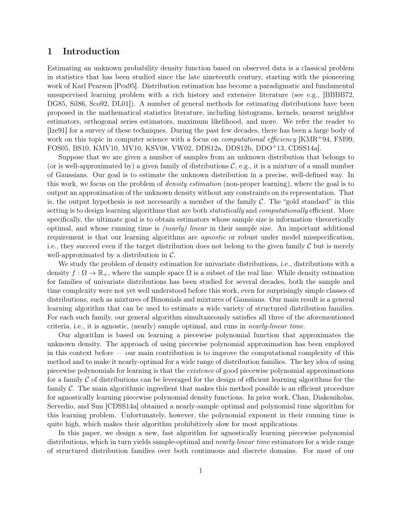
Algorithm 1 Approximating with histograms by merging.1: function ConstructHistogram(f, t, α, ε, δ)2: Draw n = Θ((αt+ log 1/δ)/ε2) samples x1 ≤ x2 ≤ . . . ≤ xn.3: Form the empirical distribution f from these samples.4: Let I0 ← [a, x1), [x1, x1], (x1, x2), . . . , (xn−1, xn), [xn, xn], (xn, b] be the initial partition.5: j ← 06: while |Ij | > 2α · t do7: Let Ij = I1,j , I2,j , . . . , Isj−1,j , Isj ,j8: for ` ∈ 1, 2, . . . , sj2 do9: I ′`,j+1 ← I2`−1,j ∪ I2`,j
10: e`,j ← e(f , I ′`,j+1)11: end for12: Let L be the set of ` ∈ 1, 2, . . . , sj2 with the αt largest errors e`,j .13: Let M be the complement of L.14: Ij+1 ←
⋃`∈LI2`−1,j , I2`,j
15: Ij+1 ← Ij+1 ∪ I ′`,j+1 | ` ∈M16: j ← j + 117: end while18: return I = Ij and the flattening fI19: end function
Theorem 10. Algorithm ConstructHistogram(f, t, α, ε, δ) draws n = O((αt+log 1/δ)/ε2) sam-ples from f , runs in time O(n (log(1/ε) + log log(1/δ))), and outputs a hypothesis h and a corre-sponding partition I of size |I| ≤ 2α · t such that with probability at least 1− δ we have
‖h− f‖1 ≤ 2 ·OPTt +4 ·OPTt + 4ε
α− 1+ ε . (2)
Proof. We start by analyzing the running time. To this end, we show that the number of intervalsdecreases exponentially with the number of iterations. In the j-th iteration, we merge all but αtintervals. Therefore,
sj+1 = αt+sj − αt
2=
3sj4
+2αt− sj
4.
Note that the algorithm enters the while loop when sj > 2αt, implying that
sj+1 <3sj4.
By construction, the number of intervals is at least αt when the algorithm exits the while loop.Therefore, the number of iterations of the while loop is at most
O(
logn
αt
)= O (log(1/ε) + log log(1/δ)) ,
which follows by substituting the value of n from the statement of the theorem. We now show thateach iteration takes time O(n). Without loss of generality, assume that we compute the A1-distanceonly over intervals ending at a data sample. For an interval J = [c, d] containing m sample points,
12

x1, . . . , xm, let Cj =(xj−x1)jn − (d−c)
n . The A1-error of f on J is given by maxCj − minCj andcan therefore be computed in time proportional to the number of sample points in the interval.Therefore, the total time of the algorithm is O(n(log(1/ε) + log log(1/δ))), as claimed.
We now proceed to bound the learning error. Let I = I1, . . . , It′ be the partition of I returnedby ConstructHistogram. The desired bound on |I| follows immediately because the algorithmterminates only when |I| ≤ 2αt. The rest of the proof is dedicated to Equation (2).
Fix h∗ ∈ Ht such that ‖h∗ − f‖1 = OPTt. Let I∗ = I∗1 , . . . , I∗t be the partition induced bythe discontinuities of h∗. Call a point at a boundary of any I∗j a jump of h∗. For any intervalJ ⊆ I, we define Γ(J) to be the number of jumps of h∗ in the interior of J . Since we drawn = Ω((αt+ log 1/δ)/ε2) samples, Corollary 4 implies that with probability at least 1− δ, we have
‖f − f‖A(2α+1)t≤ ε .
We condition on this event throughout the analysis.We split the total error into three terms based on the final partition I:
Case 1: Let F be the set of intervals in I with zero jumps in h∗, i.e., F = J ∈ I |Γ(J) = 0.
Case 2a: Let J0 be the set of intervals in I that were created in the initial partitioning step of thealgorithm and which contain a jump of h∗, i.e., J0 = J ∈ I | Γ(J) > 0 and J ∈ I0.
Case 2b: Let J1 be the set of intervals in I that contain at least one jump and were created bymerging two other intervals, i.e., J1 = J ∈ I | Γ(J) > 0 and J /∈ I0.
Notice that F , J0, and J1 form a partition of I, and thus
‖h− f‖1 = ‖h− f‖1,F + ‖h− f‖1,J0 + ‖h− f‖1,J1 .
We will bound these three terms separately. In particular, we will show:
‖h− f‖1,F ≤ 2 · ‖f − h∗‖1,F + ‖f − f‖A|F|,F , (3)
‖h− f‖1,J0 ≤ ‖f − f‖A|J0|,J0 , (4)
‖h− f‖1,J1 ≤4 ·OPTt + 4ε
α− 1+ 2 · ‖f − h∗‖1,J1 + ‖f − f‖A|J1|+t,J1 . (5)
Using these results along with the fact that ‖f − h∗‖1,F + ‖f − h∗‖1,J1 ≤ OPTt, we have
‖h− f‖1 ≤ 2 ·OPTt +4 ·OPTt + 4ε
α− 1+ ‖f − f‖A|F|,F + ‖f − f‖A|J0|,J0 + ‖f − f‖A|J1|+t,J1
(a)
≤ 2 ·OPTt +4 ·OPTt + 4ε
α− 1+ ‖f − f‖A(2α+1)t
(b)
≤ 2 ·OPTt +4 ·OPTt + 4ε
α− 1+ ε ,
where inequality (a) follows from Fact 6(d) and inequality (b) follows from the VC inequality. Thus,it suffices to prove Equations (3)–(5).
13
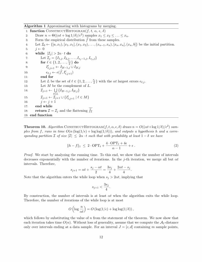
Case 1. We first consider the interval F . By the triangle inequality, we have
‖h− f‖1,F ≤ ‖f − h∗‖1,F + ‖h− h∗‖1,F .
Thus to show (3), it suffices to show that
‖h− h∗‖1,F ≤ ‖f − h∗‖1,F + ‖f − f‖A|F|,F . (6)
We prove a slightly more general version of (6) that holds over all finite sets of intervals notcontaining any jump of h∗. We will use this general version also later in our proof.
Lemma 11. Let J ∈ I`I so that Γ(J) = 0 for all J ∈ J . Let h = fJ denote the flattening of f onJ . Then
‖h− h∗‖1,J ≤ ‖f − h∗‖1,J + ‖f − f‖A`,J .
Note that this is indeed a generalization of (6) since for any point x in any interval of F , wehave h(x) = fF (x).
Proof of Lemma 11. In any interval J ∈ J with Γ(J) = 0, we have
‖h− h∗‖1,J(a)= |h(J)− h∗(J)| (b)
= |f(J)− h∗(J)|,
where (a) follows from the fact that h and h∗ are constant in J , and (b) follows from the definitionof h. Thus, we get
‖h− h∗‖1,J =∑J∈J‖h− h∗‖1,J
=∑J∈J|f(J)− h∗(J)|
(c)
≤∑J∈J|f(J)− f(J)|+
∑J∈J|f(J)− h∗(J)|
(d)
≤ ‖f − f‖A|J |,J + ‖f − h∗‖1,J
where (c) uses the triangle inequality, and (d) follows from the definition of Ak-distance.
Case 2a. Next, we analyze the error for the intervals in J0. The set I0 contains only singletonsand intervals with no sample points. By definition, only the intervals in I0 that contain no samplesmay contain a jump of h∗. The singleton intervals containing the sample points do not includejumps and are hence covered by Case 1. Since the intervals in J0 do not contain any samples, ouralgorithm assigns
h(J) = f(J) = 0
for any J ∈ J0. Hence,‖h− f‖1,J0
= ‖f‖1,J0.
14

We thus have the following sequence of (in)equalities:
‖h− f‖1,J0= ‖f‖1,J0
=∑J∈J0
|f(J)|
=∑J∈J0
|f(J)− f(J)|
≤ ‖f − f‖A|J0|,J0,
where the last step uses the definition of the Ak-norm.
Case 2b. Finally, we bound the error for intervals in J1, i.e., intervals that were created bymerging in some iteration of our algorithm and also contain jumps. As before, our first step is thefollowing triangle inequality:
‖h− f‖1,J1 ≤ ‖h− h∗‖1,J1 + ‖h∗ − f‖1,J1 .
Consider an interval J ∈ J1. Since h is constant in J and h∗ has Γ(J) jumps in J , h − h∗ hasat most Γ(J) sign changes in J . Therefore,
‖h− h∗‖1,J(a)= ‖h− h∗‖AΓ(J)+1,J
(b)
≤ ‖h− f‖AΓ(J)+1,J + ‖f − f‖AΓ(J)+1,J + ‖f − h∗‖AΓ(J)+1,J
(c)
≤ (Γ(J) + 1)‖h− f‖A1,J + ‖f − f‖AΓ(J)+1,J + ‖f − h∗‖1,J , (7)
where equality (a) follows from Fact 6(a), inequality (b) is the triangle inequality, and inequality(c) uses Fact 6(c). Finally, we bound the A1-distance in the first term above.
Lemma 12. For any J ∈ J1, we have
‖h− f‖A1,J ≤2OPTt + 2ε
(α− 1)t. (8)
Before proving the lemma, we show how to use it to complete Case 2b. Since h is the flatteningof f over J , we have that ‖h− f‖A1,J = e(f , J). Applying (7) gives:
‖h− h∗‖1,J1 =∑J∈J1
‖h− h∗‖1,J
≤∑J∈J1
((Γ(J) + 1)‖h− f‖A1,J + ‖f − f‖AΓ(J)+1,J + ‖f − h∗‖1,J
)
≤ 2 ·OPTt + 2ε
(α− 1)t·
∑J∈J1
(Γ(J) + 1)
+∑J∈J1
‖f − f‖AΓ(J)+1,J + ‖f − h∗‖1,J1
(a)
≤ 4 ·OPTt + 4ε
(α− 1)+ ‖f − f‖At+|J1|,J1 + ‖f − h∗‖1,J1
15

where inequality (a) uses the fact that Γ(J) ≥ 1 for these intervals and hence∑J∈J1
(Γ(J) + 1) ≤ 2∑J∈J1
Γ(J) ≤ 2t .
We now complete the final step by proving Lemma 12.
Proof of Lemma 12. Recall that in each iteration of our algorithm, we merge all pairs of intervalsexcept those with the αt largest errors. Therefore, if two intervals were merged, there were at leastαt other pairs of intervals with larger error. We will use this fact to bound the error on the intervalsin J1.
Consider any interval J ∈ J1, and suppose it was created in the jth iteration of the while loop ofour algorithm, i.e., J = I ′i,j+1 = I2i−1,j∪I2i,j for some i ∈ 1, . . . , sj/2. Note that this interval is notmerged again in the remainder of the algorithm. Recall that the intervals I ′i,j+1, for i ∈ 1, . . . , sj/2,are the possible candidates for merging at iteration j. Let h′ = fI′j+1
be the distribution obtainedby flattening the empirical distribution over these candidate intervals I ′j+1 = I ′1,j+1, . . . , I
′sj/2,j+1.
Note that h′(x) = h(x) for x ∈ J because J was created in this iteration.Let L be the set of candidate intervals I ′i,j+1 in the set I ′j+1 with the largest α·t errors e(f , I ′i,j+1).
Let L0 be the intervals in L that do not contain any jumps of h∗. Since h∗ has at most t jumps,|L0| ≥ (α− 1)t. Moreover, for any I ′ ∈ L0, by the triangle inequality
e(f , I ′) = ‖h′ − f‖A1,I′
≤ ‖h′ − h∗‖A1,I′ + ‖f − h∗‖A1,I′ + ‖f − f‖A1,I′
≤ ‖h′ − h∗‖A1,I′ + ‖f − h∗‖1,I′ + ‖f − f‖A1,I′ .
Summing over the intervals in L0,∑I′∈L0
e(f , I ′) ≤∑I′∈L0
(‖h′ − h∗‖A1,I′ + ‖f − h∗‖1,I′ + ‖f − f‖A1,I′
)
≤
∑I′∈L0
‖h′ − h∗‖A1,I′
+ ‖f − h∗‖1,L0 + ‖f − f‖A2αt,L0
≤
∑I′∈L0
‖h′ − h∗‖A1,I′
+ OPTt + ε , (9)
where recall that we had conditioned on the last term being at most ε throughout the analysis.Since both h and h∗ are flat on each interval I ′ ∈ L0, Lemma 11 gives∑
I′∈L0
‖h′ − h∗‖A1,I′≤ ‖f − h∗‖1,L0 + ‖f − f‖A|L0|,L0 ≤ OPTt + ε .
Plugging this into (9) gives ∑I′∈L0
e(f , I ′) ≤ 2 ·OPTt + 2ε .
16

Since J was created by merging in this iteration, we have that e(f , J) is no larger than e(f , I ′) forany of the intervals I ′ ∈ L0 (see lines 12 - 15 of Algorithm 1), and therefore e(f , J) is not largerthan their average. Recalling that |L0| ≥ (α− 1)t, we obtain
e(f , J) = ‖h′ − f‖A1,J= ‖h− f‖A1,J
≤∑
I′∈L0e(f , I ′)
(α− 1)t≤ 2OPTt + 2ε
(α− 1)t,
completing the proof of the lemma.
4.2 The general merging algorithm
We are now ready to present our general merging algorithm, which is a generalized version of thehistogram merging algorithm introduced in Section 4.1. The histogram algorithm only uses threemain properties of histogram hypotheses: (i) The number of intersections between two t-histogramhypotheses is bounded by O(t). (ii) Given an interval J and an empirical distribution f , we canefficiently find a good histogram fit to f on this interval. (iii) We can efficiently compute theA1-errors of candidate intervals.
Note that property (i) bounds the complexity of the hypothesis class and leads to a tight samplecomplexity bound while properties (ii) and (iii) are algorithmic ingredients. We can generalize thesethree notions to arbitrary classes of piecewise hypotheses as follows. Let D be a class of hypotheses.Then the generalized variants of properties (i) to (iii) are: (i) The number of intersections betweenany two hypotheses in D is bounded. (ii) Given an interval J and an empirical distribution f ,we can efficiently find the best fit to f from functions in D with respect to the Ak-distance. (iii)We can efficiently compute the Ak-distance between the empirical distribution and any hypothesisin D. Using these generalized properties, the histogram merging algorithm naturally extends toagnostically learning piecewise hypotheses where each piece is in the class D.The following definitions formally describe the aforementioned framework. We first require a mildcondition on the underlying distribution family:
Definition 13. Let D be a family of measurable functions defined over subsets of I. D is said tobe full if for each J ⊆ I, there exists a function g in D whose domain is J . Let DJ be the elementsof D whose domain is J .
Our next definition formalizes the notion of piecewise hypothesis whose components come fromD:
Definition 14. A function h : I → R is a t-piece D-function if there exists a partition of I intointervals I1, . . . , It′ with t′ ≤ t, such that for every i, 1 ≤ i ≤ t′, there exists hi ∈ DIi satisfying thath = hi on Ii. Let Dt denote the set of all t-piece D-functions.
The main property we require from our full function class D is that any two functions in Dintersect a bounded number of times. This is formalized in the definition below:
Definition 15. Let D be a full family over I and J ⊆ I. Suppose h ∈ DJ and h′ ∈ Dk for somek ≥ 1. Let h′ = h′Ii , 1 ≤ i ≤ k, for some interval partition I1, . . . , Ik of I and h′Ii ∈ DIi . Let sdenote the number of endpoints of the Ii’s contained in J . We say that D is d-sign restricted if thefunction h− h′ has at most (s+ 1)d sign changes on J , for any h and h′.
17
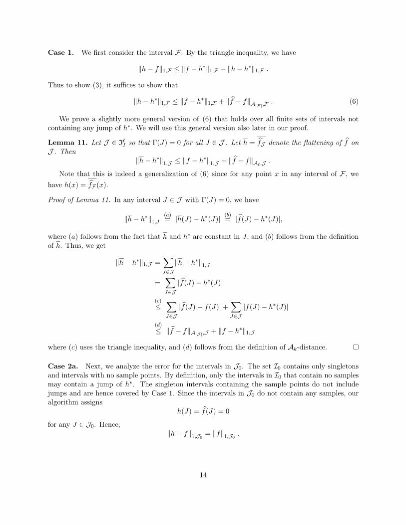
The following simple examples illustrate that histograms and more generally piecewise polyno-mial functions fall into this framework.
Example 1. Let HJ be the set of constant functions defined on J . Then if H = ∪J⊆IHJ , the set Htof t-piece H-functions is the set of piecewise constant functions on I with at most t interval pieces.(Note that this class is the set of t-histograms.)
Example 2. For J ⊆ I, we define PJ,d to be set of degree-d nonnegative polynomials on J , and
Pddef= ∪JPJ,d. Since the degree d will be fixed throughout this paper, we sometimes simply denote
this set by P. The set Pt,d of t-piece P-functions is the set of t-piecewise degree-d non-negativepolynomials. It is easy to see that this class is full over I. Since any two polynomials of degree dintersect at most d times, it is easy to see that Pd forms a d-sign restricted class.
We are now ready to formally define our general learning problem. Fix positive integers t, d anda full d-sign restricted class of functions D. Given sample access to any pdf f : I → R+, we want tocompute a good Dt approximation to f . We define OPTD,t
def= infg∈Dt ‖g− f‖1 . Our goal is to find
an O(t)-piece D-function h : I → R such that ‖h− f‖1 ≤ C ·OPTD,t +O(ε), with high probabilityover the samples, where C is a universal constant.
Our iterative merging algorithm takes as input samples from an arbitrary distribution, andoutputs an O(t)-piecewise D hypothesis satisfying the above agnostic guarantee. Our algorithmassumes the existence of two subroutines, which we call Ak-projection and Ak-computation oracles.The Ak-projection oracle was defined in Definition 7 and is restated below along with the definitionof the Ak-computation oracle (Definition 16).
Definition 7. Fix η > 0. An algorithm Op(f , J, η) is an η-approximate Ak-projection oracle forD if it takes as input an interval J and f , and returns a hypothesis h ∈ D such that
‖h− f‖Ak ≤ infh′∈D‖h′ − f‖Ak,J + η .
Definition 16. Fix η > 0. An algorithm Oc(f , hJ , J, η) is an η-approximate Ak-computation oraclefor D if it takes as input f , a subinterval J ⊆ I, and a function hJ ∈ DJ , and returns a value ξsuch that ∣∣∣‖hJ − f‖Ak,J − ξ∣∣∣ ≤ η .
We consider a d-sign restricted full family D, and a fixed η > 0. Let Rp(I) = Rp(I, f ,Op)and Rc(I) = Rc(I, f ,Oc) be the time used by the oracle Op and Oc, respectively. With a slightabuse of notation, for a collection of at most 2n intervals containing n points in the support of theempirical distribution, we also define Rp(n) and Rc(n) to be the maximum time taken by Op andOc, respectively.
We are now ready to state the main theorem of this section:
Theorem 17. Let Op and Oc be η-approximate Ak-projection and Ak-computation oracles forD. Algorithm General-Merging(f, t, α, ε, δ) draws n = O((αdt + log 1/δ)/ε2) samples, runs intime O
((Rp(n) +Rc(n)) log n
αt
), and outputs a hypothesis h and an interval partition I such that
|I| ≤ 2α · t and with probability at least 1− δ, we have
‖h− f‖1 ≤ 3 ·OPTD,t +OPTD,t + ε
α− 1+ 2ε+ η . (10)
18

In the remainder of this section, we provide an intuitive explanation of our general mergingalgorithm followed by a detailed pseudocode.
The algorithm General-Merging and its analysis is a generalization of the ConstructHis-togram algorithm from the previous subsection. More formally, the algorithm proceeds greedily,as before. We take n = O((αdt + log 1/δ)/ε2) samples x1 ≤ . . . ≤ xn. We construct I0 as in (1).In the j-th iteration, given the current partition Ij = I1,j , . . . , Isj ,j with sj intervals, consider theintervals
I ′`,j+1 = I2`−1,j ∪ I2`,j
for ` ≤ sj/2. As for histograms, we want to compute the errors in each of the new intervalscreated. To do this, we first call the Ak–projection oracle with k = d + 1 on this interval to findthe approximately best fit in D for f over these new intervals, namely:
h′`,j = Op(f , I ′`,j+1,
η
O(t)
).
To compute the error, we call the Ak–computation oracle with k = d+ 1, i.e.:
e`,j = Oc(f , h′`,j , I
′`,j+1,
η
O(t)
).
As in ConstructHistogram, we keep the intervals with the largest O(αt) errors intact andmerge the remaining pairs of intervals. We perform this procedure O(log n
αt) times and arrive atsome final partition I with O(αt) pieces. Our output hypothesis is the output of Op(f , I) over eachof the final intervals I.
The formal pseudocode for our algorithm is given in Algorithm 2. We assume that D and d areknown and fixed and are not mentioned explicitly as an input to the algorithm. Note that we runthe algorithm with η = ε so that Theorem 17 has an additional O(ε) error. The proof of Theorem 17is very similar to that of the histogram merging algorithm and is deferred to Appendix A.
4.3 Putting everything together
In Sections 5 and 6.3, we present an efficient approximateAk-projection oracle and anAk-computationoracle for Pd, respectively. We show that:
Theorem 18. Fix J ⊆ [−1, 1] and η > 0. For all k ≤ d, there is an η-approximate Ak-projectionoracle for Pd which runs in time
O
((d3 log log 1/η + sd2 + dω+2
)log2 1
η
).
where s is the number of samples in the interval J .
Theorem 19. There is an η-approximate Ak-computation oracle for Pd which runs in time O((s+d) log2(s+ d)) where s is the number of samples in the interval J .
The algorithm GeneralMerging, when used in conjunction with the oracles Op and Oc givenin Theorems 18 and 19 (for η = ε), yields Theorem 1. For this choice of oracles we have thatRp(n) +Rc(n) = O(ndω+2 log3 1/ε). This completes the proof.
19

Algorithm 2 Approximating with general hypotheses by merging.1: function General-Merging(f, d, t, α, ε, δ)2: Draw n = Θ((αdt+ log 1/δ)/ε2) samples x1 ≤ x2 ≤ . . . ≤ xn.3: Form the empirical distribution f from these samples.4: Let I0 ← [a, x1), [x1, x1], (x1, x2), . . . , (xn−1, xn), [xn, xn], (xn, b] be the initial partition.5: j ← 06: while |Ij | > 2α · t do7: Let Ij = I1,j , I2,j , . . . , Isj−1,j , Isj ,j8: for ` ∈ 1, 2, . . . , sj2 do9: I ′`,j+1 ← I2`−1,j ∪ I2`,j
10: h′`,j ← Op(f , I ′`,j+1,ε
2αt)
11: e`,j ← Oc(f , h′`,j , I ′`,j+1,ε
2αt)12: end for13: Let L be the set of ` ∈ 1, 2, . . . , sj2 with the αt largest errors e`,j .14: Let M be the complement of L.15: Ij+1 ←
⋃`∈LI2`−1,j , I2`,j
16: Ij+1 ← Ij+1 ∪ I ′`,j+1 | ` ∈M17: j ← j + 118: end while19: return I = Ij and the functions Op(f , J, ε
2αt) for J ∈ I20: end function
5 A fast Ak-projection oracle for polynomials
We now turn our attention to the Ak-projection problem, which appears as the main subroutine inthe general merging algorithm (see Section 4.2). In this section, we let E ⊂ J be the set of samplesdrawn from the unknown distribution. To emphasize the dependence of the empirical distributionon E, we denote the empirical distribution by fE in this section. Given an interval J = [a, b] anda set of samples E ⊂ J , the goal of the Ak-projection oracle is to find a hypothesis h ∈ D suchthat the Ak-distance between the empirical distribution fE and the hypothesis h is minimized. Incontrast to the merging algorithm, the Ak-projection oracle depends on the underlying hypothesisclass D, and here we present an efficient oracle for non-negative polynomials with fixed degree d. Inparticular, our Ak-projection oracle computes the coefficients c ∈ Rd+1 of a degree-d polynomial pcthat approximately minimizes the Ak-distance to the given empirical distribution fE in the intervalJ . Moreover, our oracle ensures that pc is non-negative for all x ∈ J .
At a high-level, we formulate the Ak-projection as a convex optimization problem. A key insightis that we can construct an efficient, approximate separation oracle for the set of polynomials thathave an Ak-distance of at most τ to the empirical distribution fE . Combining this separation oraclewith existing convex optimization algorithms allows us to solve the feasibility problem of checkingwhether we can achieve a given Ak-distance τ . We then convert the feasibility problem to theoptimization variant via a binary search over τ .
In order to simplify notation, we assume that the interval J is [−1, 1] and that the mass of theempirical distribution fE is 1. Note that the general Ak-projection problem can easily be convertedto this special case by shifting and scaling the sample locations and weights before passing them to
20
the Ak-projection subroutine. Similarly, the resulting polynomial can be transformed to the originalinterval and mass of the empirical distribution on this interval.4
5.1 The set of feasible polynomials
For the feasibility problem, we are interested in the set of degree-d polynomials that have an Ak-distance of at most τ to the empirical distribution fE on the interval J = [−1, 1] and are alsonon-negative on J . More formally, we study the following set.
Definition 20 (Feasible polynomials). Let E ⊂ J be the samples of an empirical distribution withfE(J) = 1. Then the set of (τ, d, k, E)-feasible polynomials is
Cτ,d,k,E :=c ∈ Rd+1 | ‖pc − fE‖Ak,J ≤ τ and pc(x) ≥ 0 for all x ∈ J
.
When d, k, and E are clear from the context, we write only Cτ for the set of τ -feasible polynomials.
Considering the original Ak-projection problem, we want to find an element c∗ ∈ Cτ∗ , whereτ∗ is the smallest value for which Cτ∗ is non-empty. We solve a slightly relaxed version of thisproblem, i.e., we find an element c for which the Ak-constraint and the non-negativity constraintare satisfied up to small additive constants. We then post-process the polynomial pc to make ittruly non-negative while only increasing the Ak-distance by a small amount.
Note that we can “unwrap” the definition of the Ak-distance and write C as an intersectionof sets in which each set enforces the constraint
∑ki=1|pc(Ii) − fE(Ii)| ≤ τ for one collection of
k disjoint intervals I1, . . . , Ik. For a fixed collection of intervals, we can then write each Ak-constraint as the intersection of linear constraints in the space of polynomials. Similarly, we canwrite the non-negativity constraint as an intersection of pointwise non-negativity constraints, whichare again linear constraints in the space of polynomials. This leads us to the following key lemma.Note that convexity of Cτ could be established more directly5, but considering Cτ as an intersectionof halfspaces illustrates the further development of our algorithm (see also the comments after thelemma).
Lemma 21 (Convexity). The set of τ -feasible polynomials is convex.4Technically, this step is actually necessary in order to avoid a running time that depends on the shape of the
unknown pdf f . Since the pdf f could be supported on a very small interval only, the corresponding polynomialapproximation could require arbitrarily large coefficients (the empirical distribution would have all samples in a verysmall interval). In that case, operations such as root-finding with good precision could take an arbitrary amountof time. In order to circumvent this issue, we make use of the real-RAM model to rescale our samples to [−1, 1]before processing them further. Combined with the assumption of unit probability mass, this allows us to bound thecoefficients of candidate polynomials in the current interval.
5Norms give rise to convex sets and the set of non-negative polynomials is also convex.
21

Proof. From the definitions of Cτ and the Ak-distance, we have
Cτ = c ∈ Rd+1 | ‖pc − fE‖Ak,J ≤ τ and pc(x) ≥ 0 for all x ∈ J
= c ∈ Rd+1 | supI∈IkJ
∑I∈I|pc(I)− fE(I)| ≤ τ ∩ c ∈ Rd+1 | pc(x) ≥ 0 for all x ∈ J
=⋂I∈IkJ
c ∈ Rd+1 |∑I∈I|pc(I)− fE(I)| ≤ τ ∩
⋂x∈Jc ∈ Rd+1 | pc(x) ≥ 0
=⋂I∈IkJ
⋂ξ∈−1,1k
c ∈ Rd+1 |k∑i=1
ξi(pc(Ii)− fE(Ii)) ≤ τ ∩⋂x∈Jc ∈ Rd+1 | pc(x) ≥ 0 .
In the last line, we used the notation I = I1, . . . , Ik. Since the intersection of a family of convexsets is convex, it remains to show that the individual Ak-distance sets and non-negativity sets areconvex. Let
M =⋂I∈IkJ
⋂ξ∈−1,1k
c ∈ Rd+1 |k∑i=1
ξi(pc(Ii)− fE(Ii)) ≤ τ
N =⋂x∈Jc ∈ Rd+1 | pc(x) ≥ 0 .
We start with the non-negativity constraints encoding the set N . For a fixed x ∈ J , we canexpand the constraint pc(x) ≥ 0 as
d∑i=0
ci · xi ≥ 0 ,
which is clearly a linear constraint on the ci. Hence, the set c ∈ Rd+1 | pc(x) ≥ 0 is a halfspacefor a fixed x and thus also convex.
Next, we consider the Ak-constraints∑k
i=1 ξi(pc(Ii) − fE(Ii)) ≤ τ for the set M. Since theintervals I1, . . . , Ik are now fixed, so is fE(Ii). Let αi and βi be the endpoints of the interval Ii, i.e.,Ii = [αi, βi]. Then we have
pc(Ii) =
∫ βi
αi
pc(x) dx = Pc(βi)− Pc(αi) ,
where Pc(x) is the indefinite integral of Pc(x), i.e.,
Pc(x) =d∑i=0
ci ·xi+1
i+ 1.
So for a fixed x, Pc(x) is a linear combination of the ci. Consequently∑k
i=1 ξipc(Ii) is also a linearcombination of the ci, and hence each set in the intersection definingM is a halfspace. This showsthat Cτ is a convex set.
It is worth noting that the set N is a spectrahedron (the feasible set of a semidefinite program)because it encodes non-negativity of a univariate polynomial over a fixed interval. After restricting
22

the set of coefficients to non-negative polynomials, we can simplify the definition of the Ak-distance:it suffices to consider sets of intervals with endpoints at the locations of samples (see Lemma 37).Hence, we can replace the supremum in the definition ofM by a maximum over a finite set, whichshows that Cτ is also a spectrahedron. This suggests that the Ak-projection problem could be solvedby a black-box application of an SDP solver. However, this would lead to a running time that isexponential in k because there are more than
(|E|2k
)possible sets of intervals. While the authors of
[CDSS14] introduce an encoding of the Ak-constraint with fewer linear inequalities, their approachincreases the number of variables in the optimization problem to depend polynomially on 1
ε , whichleads to a super-linear running time.
Instead of using black-box SDP or LP solvers, we construct an algorithm that exploits additionalstructure in the Ak-projection problem. Most importantly, our algorithm separates the dimensionof the desired degree-d polynomial from the number of samples (or equivalently, the error parameterε). This allows us to achieve a running time that is nearly-linear for a wide range of distributions.Interestingly, we can solve our SDP significantly faster than the LP which has been proposed in[CDSS14] for the same problem.
5.2 Separation oracles and approximately feasible polynomials
In order to work with the large number of Ak-constraints efficiently, we “hide” this complexity fromthe convex optimization procedure by providing access to the constraints only through a separationoracle. As we will see in Section 6, we can utilize the structure of the Ak-norm and implement sucha separation oracle for the Ak-constraints in nearly-linear time. Before we give the details of ourseparation oracle, we first show how we can solve the Ak-projection problem assuming that we havesuch an oracle. We start by formally defining our notions of separation oracles.
Definition 22 (Separation oracle). A separation oracle O for the convex set Cτ is a function thattakes as input a coefficient vector c ∈ Rd+1 and returns one of the following two results:
1. “yes” if c ∈ Cτ .
2. a separating hyperplane y ∈ Rd+1. The hyperplane y must satisfy yT c′ ≤ yT c for all c′ ∈ Cτ .
For general polynomials, it is not possible to perform basic operations such as root finding exactly,and hence we have to resort to approximate methods. This motivates the following definition of anapproximate separation oracle. While an approximate separation oracle might accept a point c thatis not in the set Cτ , the point c is then guaranteed to be close to Cτ .
Definition 23 (Approximate separation oracle). A µ-approximate separation oracle O for the setCτ = Cτ,d,k,E is a function that takes as input a coefficient vector c ∈ Rd+1 and returns one of thefollowing two results, either “yes” or a hyperplane y ∈ Rd+1.
1. If O returns “yes”, then ‖pc − fE‖Ak,J ≤ τ + 2µ and pc(x) ≥ −µ for all x ∈ J .
2. If O returns a hyperplane, then y is a separating hyperplane; i.e. the hyperplane y must satisfyyT c′ ≤ yT c for all c′ ∈ Cτ .
In the first case, we say that pc is a 2µ-approximately feasible polynomial.
23

Note that in our definition, separating hyperplanes must still be exact for the set Cτ . Althoughour membership test is only approximate, the exact hyperplanes allow us to employ several existingseparation oracle methods for convex optimization. We now formally show that many existingmethods still provide approximation guarantees when used with our approximate separation oracle.
Definition 24 (Separation Oracle Method). A separation oracle method (SOM) is an algorithmwith the following guarantee: let C be a convex set that is contained in a ball of radius 2L. Moreover,let O be a separation oracle for the set C. Then SOM(O, L) returns one of the following two results:
1. a point x ∈ C.
2. “no” if C does not contain a ball of radius 2−L.
We say that an SOM is canonical if it interacts with the separation oracle in the following way:the first time the separation oracle returns “yes” for the current query point x, the SOM returns thepoint x as its final answer.
There are several algorithms satisfying this definition of a separation oracle method, e.g., theclassical Ellipsoid method [Kha79] and Vaidya’s cutting plane method [Vai89]. Moreover, all ofthese algorithms also satisfy our notion of a canonical separation oracle method. We require thistechnical condition in order to prove that our approximate separation oracles suffice. In particular,by a straightforward simulation argument, we have the following:
Theorem 25. Let M be a canonical separation oracle method, and let O be a µ-approximateseparation oracle for the set Cτ = Cτ,d,k,E. Moreover, let L be such that Cτ is contained in a ball ofradius 2L. ThenM(O, L) returns one of the following two results:
1. a coefficient vector c ∈ Rd+1 such that ‖pc − fE‖Ak,J ≤ τ + 2µ and pc(x) ≥ −µ for all x ∈ J .
2. “no” if C does not contain a ball of radius 2−L.
5.3 Bounds on the radii of enclosing and enclosed balls
In order to bound the running time of the separation oracle method, we establish bounds on theball radii used in Theorem 25.
Upper bound When we initialize the separation oracle method, we need a ball of radius 2L
that contains the set Cτ . For this, we require bounds on the coefficients of polynomials which arebounded in L1 norm. Bounds of this form were first established by Markov [Mar92].
Lemma 26. Let pc be a degree-d polynomial with coefficients c ∈ Rd+1 such that p(x) ≥ 0 forx ∈ [−1, 1] and
∫ 1−1 p(x) dx ≤ α, where α > 0. Then we have
|ci| ≤ α · (d+ 1)2 · (√
2 + 1)d for all i = 0, . . . , d .
This lemma is well-known, but for completeness, we include a proof in Appendix B. Using thislemma, we obtain:
24

Theorem 27 (Upper radius bound). Let τ ≤ 1 and let A be the (d+1)-ball of radius r = 2Lu where
Lu = d log(√
2 + 1) +3
2log d+ 2 .
Then Cτ,d,k,E ⊆ A.
Proof. Let c ∈ Cτ,d,k,E . From basic properties of the L1- and Ak-norms, we have∫ 1
−1pc dx = ‖pc‖1,J = ‖pc‖Ak,J ≤ ‖fE‖Ak,J + ‖pc − fE‖Ak,J ≤ 1 + τ ≤ 2 .
Since pc is also non-negative on J , we can apply Lemma 26 and get
|ci| ≤ 2 · (d+ 1) · (√
2 + 1)d for all i = 0, . . . , d .
Note that the above constraints define a hypercube B with side length s = 4 · (d+ 1) · (√
2 + 1)d.The ball A contains the hypercube B because r =
√d+ 1 · s is the length of the longest diagonal
of B. This implies that Cτ,d,k,E ⊆ B ⊆ A.
Lower bound Separation oracle methods typically cannot directly certify that a convex set isempty. Instead, they reduce the volume of a set enclosing the feasible region until it reaches acertain threshold. We now establish a lower bound on volumes of sets Cτ+η that are feasible by atleast a margin η in the Ak-distance. If the separation oracle method cannot find a small ball inCτ+η, we can conclude that achieving an Ak-distance of τ is infeasible.
Theorem 28 (Lower radius bound). Let η > 0 and let τ be such that Cτ = Cτ,d,k,E is non-empty.Then Cτ+η contains a ball of radius r = 2−L` , where
L` = log4(d+ 1)
η.
Proof. Let c∗ be the coefficients of a feasible polynomial, i.e., c∗ ∈ Cτ . Moreover, let c be such that
ci =
c∗0 + η
4 if i = 0
c∗i otherwise.
Since pc∗ is non-negative on J , we also have pc(x) ≥ η4 for all x ∈ J . Moreover, it is easy to see that
shifting the polynomial pc∗ by η4 changes the Ak-distance to fE by at most η
2 because the intervalJ has length 2. Hence, ‖pc − fE‖Ak,J ≤ τ + η
2 and so c ∈ Cτ+η. We now show that we can perturbthe coefficients of c slightly and still stay in the set of feasible polynomials Cτ+η.
Let ν = η4(d+1) and consider the hypercube
B = c′ ∈ Rd+1 | c′i ∈ [ci − ν, ci + ν] for all i .
25

Note that B contains a ball of radius ν = 2−L` . First, we show that pc′(x) ≥ 0 for all x ∈ J andc′ ∈ B. We have
pc′(x) =d∑i=0
c′ixi
=d∑i=0
cixi +
d∑i=0
(c′i − ci)xi
≥ pc(x)−d∑i=0
ν|xi|
≥ η
4− (d+ 1) · ν
≥ 0 .
Next, we turn our attention to the Ak-distance constraint. In order to show that pc′ also achievesa good Ak-distance, we bound the L1-distance to pc.
‖pc(x)− pc′(x)‖1,J =
∫ 1
−1|pc(x)− pc′(x)|dx
≤∫ 1
−1
d∑i=0
ν · |xi|dx
≤∫ 1
−1(d+ 1)ν dx
= 2(d+ 1)ν
≤ η
2.
Therefore, we get
‖pc′ − fE‖Ak,J ≤ ‖pc′ − pc‖Ak,J + ‖pc − fE‖Ak,J≤ ‖pc′ − pc‖1,J + τ +
η
2≤ τ + η .
This proves that c′ ∈ Cτ+η and hence B ⊆ Cτ+η.
5.4 Finding the best polynomial
We now relate the feasibility problem to our original optimization problem of finding a non-negativepolynomial with minimal Ak-distance. For this, we perform a binary search over the Ak-distanceand choose our error parameters carefully in order to achieve the desired approximation guarantee.See Algorithm 3 for the corresponding pseudocode.
The main result for our Ak-oracle is the following:
Theorem 29. Let η > 0 and let τ∗ be the smallest Ak-distance to the empirical distribution fEachievable with a non-negative degree-d polynomial on the interval J , i.e., τ∗ = minh∈PJ,d‖h −
26

Algorithm 3 Finding polynomials with small Ak-distance.1: function FindPolynomial(d, k, E, η)2: . Initial definitions3: Let η′ = η
15 .4: Let Lu = d log(
√2 + 1) + 3
2 log d+ 2.5: Let L` = log 4(d+1)
2η′ .6: Let L = max(Lu, L`).7: LetM be a canonical separation oracle method.8: Let Oτ be an η′-approximate separation oracle
for the set of (τ, d, k, E)-feasible polynomials.
9: τ` ← 010: τu ← 111: while τu − τ` ≥ η′ do12: τm ← τ`+τu
213: τ ′m ← τm + 2η′
14: if M(Oτ ′m , L) returned a point then15: τu ← τm16: else17: τ` ← τm . Cτm′ does not contain a ball of radius 2−L and hence Cτm is empty.18: end if19: end while20: c′ ←M(Oτu+10η′ , L) . Find final coefficients.21: c0 ← c′0 + η′ and ci ← c′i for i 6= 0 . Ensure non-negativity.22: return c23: end function
27

fE‖Ak,J . Then FindPolynomial returns a coefficient vector c ∈ Rd+1 such that pc(x) ≥ 0 for allx ∈ J and ‖pc − fE‖Ak,J ≤ τ
∗ + η.
Proof. We use the definitions in Algorithm 3. Note that τ∗ is the smallest value for which Cτ∗ =Cτ∗,d,k,E is non-empty. First, we show that the binary search maintains the following invariants:τ` ≤ τ∗ and there exists a 4η′-approximately τu-feasible polynomial. This is clearly true at thebeginning of the algorithm: (i) Trivially, τ∗ ≥ 0 = τ`. (ii) For c = (0, 0, · · · , 0)T , we have ‖pc −fE‖Ak,J ≤ 1 = τu and pc(x) ≥ 0, so pc is τu-feasible (and hence also approximately τu-feasible).
Next, we consider the two cases in the while-loop:
1. If the separation oracle method returns a coefficient vector c such that the polynomial pc is 2η′-approximately τ ′m-feasible, then pc is also 4η′-approximately τm-feasible because τ ′m = τm+2η′.Hence, the update of τu preserves the loop invariant.
2. If the separation oracle method returns that Cτ ′m does not contain a ball of radius 2−L, thenτm must be empty (by the contrapositive of Theorem 28). Hence, we have τ∗ ≥ τm and theupdate of τ` preserves the loop invariant.
We now analyze the final stage of FindPolynomial after the while-loop. First, we show thatCτu+8η′ is non-empty by identifying a point in the set. From the loop invariant, we know that thereis a coefficient vector v′ such that pv′ is a 4η′-approximately τu-feasible polynomial. Consider v withv0 := v′0 + 2η′ and vi := v′i for i 6= 0. Then we have
‖pv − pv′‖1,J =
∫ 1
−1|pv(x)− pv′(x)| dx =
∫ 1
−12η′ dx = 4η′ .
Hence, we also get
‖pv − fE‖Ak,J(a)
≤ ‖pv − pv′‖Ak,J + ‖pv′ − fE‖Ak,J(b)
≤ ‖pv − pv′‖1,J + τu + 4η′ ≤ τu + 8η′ .
We used the triangle inequality in (a) and the fact that pv′ is 4η′-approximately τu-feasible in (b).Moreover, we have pv′(x) ≥ −2η′ for all x ∈ J and thus pv(x) ≥ 0 for all x ∈ J . This shows thatCτu+8η′ is non-empty because v ∈ Cτu+8η′ .
Finally, consider the last run of the separation oracle method in line 20 of Algorithm 3. SinceCτu+8η′ is non-empty, Theorem 28 shows that Cτu+10η′ contains a ball of radius 2−L. Hence, the sep-aration oracle method must return a coefficient vector c′ ∈ Rd+1 such that pc′ is 2η′-approximatelyτu + 10η′-feasible. Using a similar argument as for v, we can make pc′ non-negative while increasingits Ak-distance to fE by only 2η′, i.e., we can show that pc(x) ≥ 0 for all x ∈ J and that
‖pc − fE‖Ak,J ≤ τu + 14η′ .
Since τu − τ` ≤ η′ and τ` ≤ τ∗, we have τu ≤ τ∗ + η′. Therefore, τu + 14η′ ≤ τ∗ + 15η′ = τ∗ + η,which gives the desired bound on ‖pc − fE‖Ak,J .
In order to state a concrete running time, we instantiate our algorithm FindPolynomial withVaidya’s cutting plane method as the separation oracle method. In particular, Vaidya’s algorithmruns in time O(TdL+ dω+1L) for a feasibility problem in dimension d and ball radii bounds of 2L
and 2−L, respectively. T is the cost of a single call to the separation oracle and ω is the matrix-multiplication constant. Then we get:
28

Theorem 30. Let O be an η14 -approximate separation oracle that runs in time T . Then Find-
Polynomial has time complexity O((Td2 + dω+2) log2 1η ).
Proof. The running time of FindPolynomial is dominated by the binary search. It is easy tosee that the binary search performs O(log 1
η ) iterations, in which the main operation is the callto the separation oracle method. Our bounds on the ball radii in Theorems 27 and 28 implyL = O(d + log 1
η ). Combining this with the running time bound for Vaidya’s algorithm gives thetime complexity stated in the theorem.
In Section 6 we describe a µ-approximate separation oracle that runs in time O(dk+d log log 1/µ+s), where s is the number of samples in the empirical distribution on the interval J . Plugging thisoracle directly into our algorithm FindPolynomial gives an η-approximate Ak-projection oraclewhich runs in time O((d3k + d3 log log 1/η + sd2 + dω+2) log2 1
η ). This algorithm is the algorithmpromised in Theorem 18.
6 The separation oracle and the Ak-computation oracle
In this section, we construct an efficient approximate separation oracle (see Definition 23) for theset Cτ over the interval J = [−1, 1]. We denote our algorithm by ApproxSepOracle. Let A bethe ball defined in Lemma 27. We will show:
Theorem 31. For all µ > 0, ApproxSepOracle(c, µ) is a µ-approximate separation oracle forCτ that runs in time O(dk + d log log 1
µ + s), where s the number of samples in J , assuming allqueries are contained in the ball A.
Along the way we also develop an approximate Ak-computation oracle ComputeAk.
6.1 Overview of ApproxSepOracle
ApproxSepOracle consists of two parts, TestNonnegBounded and AkSeparator. We show:
Lemma 32. For any τ ≤ 2, given a set polynomial coefficients c ∈ A ⊂ Rd+1, the algorithmTestNonnegBounded(c, µ) runs in time O(d log2 d(log2 d+log log 1/µ)) and outputs a separatinghyperplane for Cτ or “yes”. Moreover, if there exists a point x ∈ [−1, 1] such that pc(x) < −µ, theoutput is always a separating hyperplane.
We show in the next section that whenever c /∈ Cτ the output is “yes”.
Theorem 33. Given a set of polynomial coefficients c ∈ A ⊂ Rd+1 such that pc(x) ≥ −µ for allx ∈ [−1, 1], there is an algorithm AkSeparator(c, µ) that runs in time O(dk+ (s+ d) log2(s+ d))and either outputs a separating hyperplane for c from Cτ or returns “yes”. Moreover, if ‖pc−fE‖Ak >τ + 2µ, the output is always a separating hyperplane.
29

ApproxSepOracle given TestNonnegBounded and AkSeparator Given Test-NonnegBounded and AkSeparator, it is straightforward to design ApproxSepOracle.
We first run TestNonnegBounded(c, µ). If it outputs a separating hyperplane, we returnthe hyperplane. Otherwise, we run AkSeparator(c, µ), and again if it outputs a separatinghyperplane, we return it. If none of these happen, we return “yes”. Lemma 32 and Theorem 33imply that ApproxSepOracle is correct and runs in the claimed time:
O(d log2 d(log2 d+ log log 1/µ)) + O(dk + (s+ d) log2(s+ d)) = O(dk + d log log 1/µ+ s) .
In the following sections, we prove Lemma 32 and Theorem 33. In Section 6.2 we describeTestNonnegBounded and prove Lemma 32, and in Section 6.3 we describe AkSeparator andprove Theorem 33.
6.2 Testing non-negativity and boundedness
Formally, the problem we solve here is the following testing problem:
Definition 34 (Approximate non-negativity test). An approximate non-negativity tester is an al-gorithm satisfying the following guarantee. Given a polynomial p =
∑di=0 cix
i with maxi|ci| ≤ αand a parameter µ > 0, return one of two results:
• a point x ∈ [−1, 1] at which p(x) < −µ/2.
• “OK”.
Moreover, it must return the first if there exists a point x′ ∈ [−1, 1] so that p(x′) < −µ.
Building upon the classical polynomial root-finding results of [Pan01], we show:
Theorem 35. Consider p and µ from Definition 34. Then there exists an algorithm TestNonneg(p, µ)that is an approximate non-negativity tester and runs in time
O(d log2 d · (log2 d+ log logα+ log log(1/µ))) ,
where α is a bound on the coefficients of p.
This theorem is proved in Section B.2.We have a bound on the coefficients c since we may assume that c ∈ A, and so we can use this
algorithm to efficiently test non-negativity as we require. Our algorithm TestNonnegBoundedsimply runs TestNonneg(pc, µ). If this returns ”yes”, then TestNonnegBounded outputs ”yes”.Otherwise, TestNonneg(pc, µ) outputs a point x ∈ [−1, 1] such that pc(x) ≤ −µ/2. In that case,TestNonnegBounded returns the hyperplane defined by y = −(1, x, x2, . . . , xd)T , i.e., pc(x) =−yT c. Note that for all c′ ∈ Cτ we have pc′(y) ≥ 0 and hence yT c′ ≤ 0. This shows that
yT c′ ≤ 0 <µ
2≤ −pc(x) = yT c
as desired.
30
Proof of Lemma 32. The correctness of this algorithm follows from the correctness of TestNonneg.We therefore only bound the running time. The worst-case runtime of this algorithm is exactly theruntime of TestNonneg(pc, µ) for any c ∈ A. Since we run TestNonneg(pc, µ) only whenmaxi∈[d] |ci| ≤ 2Lu = 2O(d) (see Theorem 27) , the runtime of TestNonneg(pc, µ) is
O(d log2 d(log2 d+ log log 1/µ)),
as claimed.
6.3 An Ak-computation oracle
We now consider the Ak-distance computation between two functions, one of which is a polynomialand the other an empirical distribution. In this subsection, we describe an algorithm ComputeAk,and show:
Theorem 36. Given a polynomial p such that p(x) ≥ −µ for all x ∈ [−1, 1] and an empiricaldistribution f supported on s points, for any k ≤ d, ComputeAk(p, f , k) runs in time O((s +d) log2(s+ d)), and computes a value v ∈ R+ such that |v − ‖p− f‖Ak | ≤ 2µ and a set of intervalsI1, . . . , Ik so that
k∑i=1
∣∣∣p(Ii)− f(Ii)∣∣∣ = v .
Note that this theorem immediately implies Theorem 19.
AkSeparator given ComputeAk: Before describing ComputeAk, we show how to designAkSeparator satisfying Theorem 33 given such a subroutine ComputeAk.
The algorithm AkSeparator is as follows: we run ComputeAk(pc, f , k), let v be its estimatefor ‖pc − f‖Ak , and let I1, . . . , Ik be the intervals it produces. If v ≤ τ , we output “yes”.
Otherwise, suppose
v =
k∑i=1
|pc(Ii)− f(Ii)| > τ .
Note that if ‖pc − f‖Ak > τ + 2µ, this is guaranteed to happen since v differs from ‖pc − f‖Ak byat most 2µ. Let σi = sign(pc(Ii)− f(Ii)). Let Ii = [ai, bi]. Then
k∑i=1
|pc(Ii)− f(Ii)| =k∑i=1
σi
(∫ bi
ai
pc(x) dx− f(Ii)
)
=k∑i=1
σi
d∑j=0
1
j + 1
(bj+1i − aj+1
i
)cj − f(Ii)
,
and therefore,k∑i=1
σi
d∑j=0
1
j + 1
(bj+1i − aj+1
i
)cj > τ +
k∑i=1
σif(Ii) . (11)
Note that the left hand side is linear in c when we fix σi, and this is the separating hyperplaneAkSeparator returns in this case.
31

Proof of Theorem 33 given Theorem 36. We first argue about the correctness of the algorithm. If‖pc − f‖Ak ≥ τ + 2µ, then ComputeAk guarantees that
v =i∑i=1
|pc(Ii)− f(Ii)| > τ .
Consider the hyperplane constructed in (11). For any c′ ∈ Cτ
k∑i=1
σi
d∑j=0
1
j + 1
(bj+1i − aj+1
i
)c′j − f(Ii)
≤ k∑i=1
∣∣∣∣∣∣d∑j=0
1
j + 1
(bj+1i − aj+1
i
)c′j − f(Ii)
∣∣∣∣∣∣=
d∑j=0
∣∣∣pc′(Ij)− f(Ii)∣∣∣
≤ |pc′ − f‖Ak ≤ τ ,
where the last inequality is from the definition of Cτ . Therefore this is indeed a separating hyperplanefor c and Cτ . Moreover, given I1, . . . , Ik and v, this separating hyperplane can be computed in timeO(dk). Thus the entire algorithm runs in time O(dk + (s+ d) log2(s+ d) as claimed.
6.3.1 A Reduction from Continuous to Discrete
We first show that our Ak–computation problem reduces to the following discrete problem: For asequence of real numbers c1, . . . , cr and an interval I = [a, b] in [r], let w(I) =
∑a≤i≤b ci. We show
that our problem reduces to the problem DiscreteAk, defined below.DiscreteAk: Given a sequence of r real numbers ciri=1 and a number k, find a set of k
disjoint intervals I1, . . . , Ik that maximizes
k∑i=1
|w(Ii)| .
We will denote the maximum value obtainable ‖ci‖Ak , i.e.,
‖ci‖Ak = maxI
∑I∈I|w(I)| ,
where the I is taken over all collections of k disjoint intervals.We will show that it is possible to reduce the continuous problem of approximately computing
the Ak distance between p and f to solving DiscreteAk for a suitably chosen sequence of lengthO(d). Suppose the empirical distribution f is supported at s points a < x1 ≤ . . . ≤ xs ≤ b in thisinterval. Let X be the support of f . Let p[α, β] =
∫ βα p(x)dx. Consider the following sequences of
length 2s+ 1:
E(i) =
1/n if i is even,
0 if i is odd., Pdisc(i) =
p[x`, x`+1] if i = 2`+ 1,
0 if i is even.,
where for simplicity we let s0 = a and ss+1 = b. The two sequences are displayed in Table 2.Then we have the following lemma:
32

i 1 2 3 4 . . . 2s 2s+ 1
E(i) 0 1n 0 1
n . . . 1n 0
Pdisc(i) p[a, x1] 0 p[x1, x2] 0 . . . 0 p[xs, b]
Table 2: The sequences E(i) and Pdisc(i).
Lemma 37. For any polynomial p so that p(x) ≥ −µ on [−1, 1]∣∣∣‖p− f‖Ak − ‖Pdisc − E‖Ak∣∣∣ < 2µ .
Moreover, given k intervals I1, . . . , Ik maximizing ‖Pdisc − E‖Ak , one can compute k intervalsJ1, . . . , Jk so that ∣∣∣∣∣
k∑i=1
∣∣∣p(Ji)− f(Ji)∣∣∣− ‖Pdisc − E‖Ak
∣∣∣∣∣ < 2µ
in time O(k).
Proof. We first show that‖p− f‖Ak ≥ ‖Pdisc − E‖Ak .
Let I1, . . . , Ik be a set of disjoint intervals in [2d+ 1] achieving the maximum on the RHS. Then itsuffices to demonstrate a set of k disjoint intervals J1, . . . , Jk in I satisfying
k∑i=1
∣∣∣p(Ji)− f(Ji)∣∣∣ ≥ k∑
i=1
|Pdisc(Ii)− E(Ii)| . (12)
We construct the Ji as follows. Fix i, and let Ii = [ai, bi]. Define Ji to be the interval fromai to bi. If ai is even (i.e., if Pdisc(ai) − E(i) has only a contribution from −E(ai)), include theleft endpoint of this interval from Ji, otherwise (i.e., if Pdisc(ai) − E(i) has only a contributionfrom Pdisc(ai)), exclude it, and similarly for the right endpoint. Then, by observation, we havePdisc(Ii)− E(Ii) = p(Ji)− f(Ji), and thus this choice of Ji satisfies (12), as claimed.
Now we show the other direction, i.e., that
‖p− f‖Ak ≤ ‖Pdisc − E‖Ak + 2µ .
Let I1, . . . , Ik denote a set of disjoint intervals in I achieving the maximum value on the LHS.It suffices to demonstrate a set of k disjoint intervals J1, . . . , Jk in I satisfying
k∑i=1
∣∣∣p(Ii)− f(Ii)∣∣∣ ≤ k∑
i=1
|Pdisc(Ji)− E(Ji)|+ 2µ . (13)
We first claim that we may assume that the endpoints of each Ii are at a point in the supportof the empirical. Let ai and bi be the left and right endpoints of Ii, respectively. Cluster theintervals Ii into groups, as follows: cluster any set of consecutive intervals Ij , . . . , Ij′ if it is thecase that p(I`) − f(I`) ≥ 0 for ` = j, . . . , j′, and [b`, a`+1] contains no points of the empirical, for
33

` = j, . . . , j′−1. Put all other intervals not clustered this way in their own group. That is, cluster aset of consecutive intervals if and only if on all of them the contribution to the LHS is non-negative,and there are no points of the empirical between them. Let the clustering be I1, . . . , Ik′ , and let Jibe the smallest interval containing all the intervals in Ij . Let ci and di denote the left and rightendpoints of Ji, respectively. Associate to each cluster a sign σi ∈ −1, 1 which is the (unique)sign of p(I) − f(I) for all I ∈ Ij . Since p(i) ≥ −µ, this clustering has the property that for anycluster Ii, we have ∣∣∣∣∣∣
∑I∈Ii
p(I)− f(I)
− (p(Ji)− f(Ji))
∣∣∣∣∣∣ ≤ µ · |Ji −⋃I∈Ij
I| .
Then, for all i, if σi = 1, take the interval I ′i = (xj , x`) where xj is the largest point in X sothat xj ≤ ci, and where x` is the smallest point in X so that x` ≥ di. Then since p ≥ µ on [−1, 1]
and the new interval contains no points in the support of f which are not in ∪I∈IjI or Ji, we have
p(I ′i)− f(I ′i) ≥ p(Ji)− f(I ′i)− µ∣∣I ′i − Ji∣∣ ≥
∑I∈Ii
p(I)− f(I)
− µ|Ji − ∪I∈IjI| − µ ∣∣I ′i − Ji∣∣ .Alternatively, if σi < 0, take the interval I ′i = [xj , x`] where xj is the smallest point in X so thatxj ≥ ci and x` is the largest point in X so that x` ≤ di. By the analogous reasoning as before wehave that p(I ′i)− f(I ′i) ≤ p(Ji)− f(Ji) +µ|Ji|,6 and therefore |p(I ′i)− f(I ′i)|+µ|Ii| ≥ |p(Ji)− f(Ji)|.Thus,
k∑i=1
∣∣∣p(Ii)− f(Ii)∣∣∣ ≤ k′∑
i=1
(|p(I ′i)− f(I ′i)|+ µ|Ji − ∪I∈IjI|+ µ
∣∣I ′i − Ji∣∣)
≤k′∑i=1
∣∣∣p(I ′i)− f(I ′i)∣∣∣+ 2µ .
since∑k′
i=1
(|Ji − ∪I∈IjI + µ |I ′i − Ji|
)≤ 2 as the intervals in the sum are disjoint subintervals in
[−1, 1].Now it is straightforward to define the Ji. Namely, for each Ii with endpoints xi1 ≤ xi2 so that
xi1 , xi2 ∈ X , define
Ji =
[i1, i2] if xi1 , xi2 ∈ X ;
[i1 + 1, i2] if xi1 6∈ X and xi2 ∈ X ;
[i1, i2 − 1] if xi1 ∈ X and xi2 6∈ X ;
[i1 + 1, i2 − 1] if xi1 , xi2 6∈ X .
One can check that with this definition of the Ji, we have p(Ii)− f(Ii) = Pdisc(Ji)−E(Ji); moreover,all the Ji are discrete and thus this choice of Ji satisfies (6.3.1).
Moreover, the transformation claimed in the lemma is the transformation provided in the firstpart of the argument. It is clear that this transformation is computable in a single pass throughthe intervals I1, . . . , Ik. This completes the proof.
6Since each cluster with negative sign has exactly a single interval in the original partition, notationally we willnot distinguish between Ji and the one interval in the original partition in Ii, when σi = −1.
34

6.3.2 Description of ComputeDiscreteAk
For the rest of this section we focus on solving DiscreteAk. A very similar problem was consideredin [Csu04] who showed an algorithm for the problem of computing the set of k disjoint intervalsI1, . . . , Ik maximizing ∣∣∣∣∣
k∑i=1
w(Ii)
∣∣∣∣∣which runs in time O(d ·minlog d, k) time. We require a modified version of this algorithm whichwe present and analyze below. We call our variant ComputeDiscreteAk.
Here is an informal description of ComputeDiscreteAk. First, we may assume the originalsequence is alternating in sign, as otherwise we may merge two consecutive numbers without con-sequence. We start with the set of intervals I0 = I0,1 ≤ . . . ≤ I0,r, where I0,i = [ci, ci] contains onlythe point ci. We first compute J0 and m0, where J0 is the set of k intervals I in I0 with largest|w(I)|, and m0 =
∑I∈J0
|w(I)|. Iteratively, after constructing Ii = Ii,1, . . . , Ii,r, we constructIi+1 by finding the set Ii,j with minimal |w(Ii,j)| amongst all intervals in Ii, and merging it withboth of its neighbors (if it is the first or last interval and so only has one neighbor, instead discardit), that is,
Ii+1 = Ii,1, . . . , Ii,j−2, Ii,j−1 ∪ Ii,j ∪ Ii,j+1, Ii,j+2, . . . , Ii,ri .
We then compute Ji+1 and mi+1 where Ji+1 is the set of k intervals I in Ii+1 with largest |w(I)|,and mi+1 =
∑I∈Ji+1
|w(I)|. To perform these operations efficiently, we store the weights of theintervals we create in priority queues. We repeat this process until the collection of intervals I`has ≤ k intervals. We output Ji and wi, where wi is the largest amongst all wi′ computed in anyiteration. An example of an iteration of the algorithm is given in Figure 1, and the formal definitionof the algorithm is in Algorithm 4.
Iteration i :0.8 −0.5 0.4 −0.1 0.3−0.4 0.5
Iteration i+ 1 :0.8 −0.5 0.6 −0.4 0.5
Figure 1: An iteration of ComputeDiscreteAk. The numbers denote the weight of each interval.The interval with smallest weight (in absolute value) is chosen and merged with adjacent intervals.Note that if weights are of alternating signs at the start, then they are of alternating signs at eachiteration.
The following runtime bound can be easily verified:
Theorem 38. Given ciri=1, ComputeDiscreteAk(ciri=1, k) runs in time O(r ·minlog r, k).
The nontrivial part of the analysis is correctness.
Theorem 39. Given ciri=1 and k, the set of intervals returned by the algorithm Compute-DiscreteAk(ciri=1, k) solves the problem DiscreteAk.
35

Algorithm 4 Computing the discrete Ak norm of a sequence.1: function ComputeDiscreteAk(ciri=1, k)2: Let I0 ← [c1, c1], [c2, c2], . . . , [cr, cr] be the initial set of intervals.3: Let Q be an empty priority queue.4: for I ∈ I0 do5: Q.push(I, w(I))6: end for7: i← 08: while |Ii| > k do9: Let I ← Q.deleteMin().
10: if I is not the leftmost or rightmost interval then11: Let Ileft and Iright be its left and right neighbors, respectively.12: Q.remove(Ileft)13: Q.remove(Iright)14: Let I ′ = Ileft ∪ I ∪ Iright15: Q.push(I ′, w(I ′))16: end if17: i← i+ 118: Let Ii be the elements of Q19: Let Ji be the k intervals in Ii with maximum weight20: Let wi =
∑I∈Ji w(I)
21: end while22: return wj and Jj where wj satisfies wj ≥ wi for all i.23: end function
Proof. Our analysis follows the analysis in [Csu04]. We call any I∗ which attains the maximumfor the DiscreteAk problem a maximal subset, or maximal for short. For any two collections ofdisjoint intervals I ′, I ′′ in [r], we say that I ′ is contained in I ′′ if all the boundary points of intervalsin I ′ are also boundary points of intervals in I ′′. Figure 2 shows an example of two collections ofintervals, one contained in the other. If there is a maximal I∗ that is contained in I we say thatI contains a maximal subset. We say that I ′ is atomic with respect to I ′′ if every interval in I ′ isalso in I ′′. Figure 3 gives an example of two collections of intervals, one atomic with respect to theother. If there is a maximal I∗ that is atomic with respect to I then we say that the maximum isatomic with respect to I.
I ′ :
I ′′ :
Figure 2: I ′ is contained in I ′′ since each boundary point of all intervals in I ′ are boundary pointsof some interval in I ′′.
We will prove the following invariant of our algorithm:
36

I ′ :
I ′′ :
Figure 3: I ′ is atomic with respect to I ′′, since each interval in I ′ is also an interval in I ′′.
Lemma 40. For any i ≥ 0, if Ii contains a maximal subset, then either the maximum is atomicwith respect to Ii or Ii+1 contains a maximal subset.
Before we prove this lemma, let us see how it suffices to prove Theorem 39. Now the set I0
contains a maximal subset. By induction and Lemma 40, for all i, as long as the maximum is notatomic with respect to Ii, Ii+1 contains a maximal subset. ComputeDiscreteAk stops iteratingat iteration if if Iif has at most k intervals. At this point either the maximum was atomic withrespect to some Ii, or Iif contains a maximal subset. Let I∗ be any maximal subset it contains.We observe that ∑
I∈I∗|w(I)| ≤
∑I∈Iif
|w(I)| ,
and moreover, Iif has k pieces, so Iif is itself maximal, and is atomic with respect to itself.Thus, there is some i so that Ii contains a maximal subset that is atomic with respect to Ii.
Call this maximal subset I∗. But then since it is atomic with respect to Ii, we have that∑I∈I∗|w(I)| ≤
∑I∈Ji
|w(I)| = mi ,
since Ji is chosen to maximize the sum over all sets of k intervals which are atomic with respect toIi. Since I∗ achieves the maximum for DiscreteAk, we conclude that mi is indeed the maximum.Thus whatevermi′ we output is also the maximum, and its Ji′ attains the maximum. This completesthe proof of Theorem 39 assuming Lemma 40.
We now prove Lemma 40.
Proof of Lemma 40. It suffices to show that if Ii contains a maximal subset, but the maximum isnot atomic with respect to Ii, then Ii+1 also contains a maximal subset. Thus, let I∗ be such that
1. I∗ is maximal
2. I∗ is contained in Ii, and
3. there is no I∗1 6= I∗ satisfying conditions (1) and (2) so that every interval in I∗1 is containedin some interval in I∗.
Such an I∗ clearly exists by the assumption on Ii. Note that I∗ cannot be atomic with respect toIi. By observation we may assume that no interval I ′ in a maximal subset will ever end on a pointa so that w(I ′) and ca have different signs, since otherwise we can easily modify the partition tohave this property while still maintaining properties (1)-(3). More generally, we may assume theredoes not exist an interval I ′′ contained in I ′ with right endpoint equal to I ′’s right endpoint (resp.left endpoint equal to I ′’s left endpoint) so that w(I ′) and w(I ′′) have different signs.
37

Let Ij = [β2, β3] be the interval in Ii with minimal |w(I)| amongst all I ∈ Ii. WLOG assumethat it is not the leftmost or rightmost interval (the analysis for these cases is almost identical andso we omit it). Let β1 be the left endpoint of Ij−1 and β4 be the right endpoint of Ij+1. WLOGassume that w(Ij) < 0.
The initial partition I0 had the property that the signs of the values w(I) for I ∈ I0 alternated,and through a simple inductive argument it follows that for all Ii, the signs of the values w(I)for I ∈ Ii still alternate. Thus, we have w(Ij−1), w(Ij+1) ≥ 0. Since I∗ is not atomic, thereis some Ia ∈ I∗ which contains at least two intervals I1, I2 of Ii. Moreover, since the signs ofthe w(I) of the intervals in Ii alternate, we may assume that w(I1) and w(I2) have differentsigns. Thus, by observation, we may in fact assume that Ia contains three consecutive intervalsI1 < I2 < I3, and that w(Ia), w(I1), w(I3) have the same sign, and w(I2) has a different sign.Moreover, |w(Ij)| ≤ minw(I1), w(I2), w(I3). Moreover, define I1
a to be the interval which sharesa left endpoint with Ia, and which has right endpoint the right endpoint of I1, and I2
a to be theinterval which shares a right endpoint with Ia, and which has left endpoint the left endpoint of I3
(See Figure 4).
. . . . . .
. . . . . .
I∗ :
Ii :
Ia
. . .. . .I3I1 I2
I1a I2
a
Figure 4: The interval Ia, and the intervals I1, I2, and I3.
We must have that w(I1a), w(I2
a) are the same sign as w(Ia) as otherwise, say if w(I1a)’s sign was
different from w(Ia)’s sign, we would have |w(Ia)| ≤ |w(I2a)| and so the existence of the collection
of intervals I ′ = (I∗ \ Ia) ∪ I2a violates condition (3), since it is contained in Ii, and∑
I∈I′|w(I)| =
∑I∈I∗|w(I)| − |w(Ia)|+ |w(I2
a)| ≥∑I∈I∗|w(I)| ,
so it is maximal.Since I∗ is contained in Ii, the only boundary points that intervals in Ii can have in the interval
[β1, β4] are at the points βi for i ∈ 1, 2, 3, 4. There are a few cases.
Case 1 If no interval in I∗ has any boundary point at β2 or β3, then it is still contained in Ii+1,by the definition of Ii+1.
Case 2 If [β2, β3] ∈ I∗, define I ′ = (I∗ \ [β2, β3], Ia) ∪ I1a , I
2a. Then∑
I∈I′|w(I)| =
∑I∈I∗|w(I)| − |w(Ij)|+ |w(I2)| ≥
∑I∈I∗|w(I)|
by the choice of Ij , so I ′ is maximal, contained in Ii, and thus its existence violates condition (3),so this case is impossible. This is illustrated in Figure 5, where for simplicity Ia contains preciselythree intervals.
38

I∗ : . . . . . .
. . . . . .
Ia
Ii :Ijβ2 β3I1
a I2 I2a
Figure 5: When Ij is an element of I∗, we can drop it and add the intervals I1a and I2
a achieving alarger weight.
Case 3 If β3 is the right endpoint of some interval I ∈ I∗, then by the same reasoning as before,we may assume that w(I) < 0. Then, let I ′ be the interval with the same left endpoint as I but withright endpoint β1. Since then w(I ′) = w(I)−w(Ij−1)−w(Ij) ≤ w(I), the partition I ′ = I∗ \ I ∪ I ′is maximal, contained in Ii, and its existence again violates condition (3), so this case is impossible.An illustration is given in Figure 6.
I∗ : . . . . . .
. . . . . .
I
Ii :
β1
IjI ′
β3
Ij−1
β2
Figure 6: I∗ can drop I and instead take I ′ to get a larger weight.
Case 4 If β2 is the left endpoint of some interval I ∈ I∗, then analogous reasoning to that in Case3 results in a contradiction, so this case is also impossible.
Case 5a If β2 is the right endpoint of some interval I ∈ I∗, and no interval in I∗ contains Ij+1,then we know that w(I) ≥ 0. Let I ′ be the interval I ∪ Ij ∪ Ij+1. Then, the partition I ′ = I∗ \ I ∪ I ′is maximal by the same kind of reasoning as before, and I ′ is contained in Ij+1. Thus, this case ispossible and consistent with the Lemma.
Case 5b If β2 is the right endpoint of some interval I ∈ I∗ and β3 is the left endpoint ofsome interval I ′ ∈ I∗, then we know that w(I), w(I ′) ≥ 0. Let I ′′ = I ∪ Ij ∪ I ′. Define I ′ =(I∗ \ I, I ′, Ia) ∪ I ′′, I1
a , I2a. Then,∑
I∈I′|w(I)| =
∑I∈I∗|w(I)| − |w(Ij)|+ |w(I2)| ≥
∑I∈I∗|w(I)| ,
so again this is a maximal subset which is now contained in Ij+1.
Case 6 If β3 is the left endpoint of some interval in I∗, by analogous reasoning to that in Cases5a and 5b, we may conclude that in this case, the Lemma holds.
These cases encompass all possible cases, and thus we conclude that the Lemma holds, asclaimed.
39

6.3.3 Description of ComputeAk
Our algorithm ComputeAk uses Fact 41 below, produces the sequence Pdisc(i)−E(i), and computes‖Pdisc − E‖Ak using ComputeDiscreteAk.
It thus suffices to show that we can construct this sequence Pdisc(i) − E(i) efficiently when weare given the empirical distribution and the polynomial p. The only difficulty lies in efficientlycomputing the p[xi, xi+1]. This problem is equivalent to efficiently evaluating the integral of p atall the points in X , which is in turn equivalent to efficiently evaluating a degree d + 1 polynomialat s points. To do so, we use the following well-known fact:
Fact 41 ([VZGG13], p. 299 and p. 245). Let x1, . . . , xs be a set of s real numbers and let p be apolynomial of degree at most s. Then there is an algorithm that computes p(x1), . . . , p(xs) in timeO(s log2 s).
After solving the discretized version of the problem, the algorithm outputs the estimate thatComputeDiscreteAk computed and the processed version of the intervals, where the processingis the one described in Lemma 37. Thus, we have:
Proof of Theorem 36. The correctness of the algorithm follows from Lemma 37 and the argumentsgiven above. Thus it suffices to bound the running time. The time required to produce the sequencePdisc(i)−E(i) is bounded by computing the p[xi, xi+1], which can be done in time O((s+d) log2(s+d)) by Fact 41. Moreover, the running time of ComputeDiscreteAk on the sequence Pdisc(i)−E(i)is O(s log s). Hence, the running time of the overall algorithm is O((s+d) log2(s+d)), as claimed.
7 Applications
In this section, we apply our main result to obtain near optimal estimators for various classes ofstructured distributions. As described in Table 1, we consider arbitrary mixtures of well-studied dis-tribution families, including log-concave distributions, normal distributions, densities with boundednumber of modes, and density functions in Besov spaces. We also consider mixtures of discrete struc-tured distributions over an ordered domain, such as multi-modal distributions, monotone hazardrate distributions, Poisson, and Binomial distributions. For all these classes, our sample complexityand running time match the information-theoretic optimum, up to at most logarithmic factors.
We note that even though our algorithm is stated for distributions over a known finite interval,they are also applicable to distributions over the entire real line, such as (mixtures of) Gaussians orPoisson distributions. This follows from the following fact: let xmin and xmax be the smallest andlargest elements among log(1/δ)
ε2draws from any distribution. Then with probability at least 1− δ,
the distribution assigns probability mass at least 1− ε to the interval [xmin, xmax]. Thus, at a cost oflog(1/δ)
ε2samples, we may truncate the distribution and thereafter only consider this finite interval.
7.1 Mixture of log-concave distributions
For an interval I ⊆ R, a function g : I → R is called concave if for any x, y ∈ I and λ ∈ [0, 1]it holds g (λx+ (1− λ)y) ≥ λg(x) + (1 − λ)g(y). A function h : I → R+ is called log-concave ifh(x) = exp (g(x)), where g : I → R is concave. A density f is a k-mixture of log-concave densityfunctions if there exist w1, . . . , wk ≥ 0,
∑iwi = 1 and log-concave density functions f1, . . . , fk
such that f =∑wifi. The class of log concave distributions is very broad and contains the
40

class of Gaussians, uniform, exponential, Gamma, Beta, and Weibull distributions. Log-concavedistributions have received significant interest in economics and statistics [BB05, CSS10, DR09,DW13, CS13, KS14, BD14, HW15].
It was shown in [CDSS14a] that a k-mixture of log-concave density functions can be ε-approximatedin L1-norm by a t-piecewise linear density, for t = O(k/
√ε). Using this structural result, [CDSS14a]
gave a polynomial time algorithm with sample complexity O(t/ε2) = O(k/ε5/2) to agnostically learna k-mixture of log-concave distributions. This sample bound is nearly optimal, as Ω(k/ε5/2) samplesare necessary for this learning problem.
Our main result yields a sample optimal and nearly-linear time algorithm for this problem. Inparticular, this follows from a combination of Theorem 1 and a recently obtained tight structuralresult that removes the logarithmic factors from the previous construction of [CDSS14a]. In partic-ular, it is shown in [DK15] that a k-mixture of log-concave density functions can be ε-approximatedin L1-norm by a t-piecewise linear density, for t = O(k/
√ε). As a corollary, we obtain the following:
Theorem 42. There is an agnostic learning algorithm for the class of k-mixtures of log-concavedistributions over the real line that uses O(k/ε5/2) samples and runs in time O((k/ε5/2)).
7.2 Mixture of Gaussians
LetN(µ, σ2) denote the normal distribution with mean µ and variance σ2. A density f : R→ R+ is ak-mixture of Gaussians if there exist w1, . . . , wk ≥ 0,
∑iwi = 1, µ1, . . . , µk ∈ R, and σ1, . . . , σk ∈ R+
such that f =∑k
i=1wiN(µi, σ2i ).
In the theoretical computer science community, the problem of parameter estimation for Gaus-sian mixtures was initiated by [Das99]. Recent work has obtained polynomial sample and timealgorithms for this problem under the conditions of identifiability [MV10, BS10]. We remark thatlearning the parameters of a mixture of k univariate Gaussians to accuracy ε requires Ω((1/ε)6k−2)samples [HP15] .
The problem of proper learning for Gaussian mixtures has also been recently studied in [DK14,SOAJ14] who obtain algorithms that draw O(k/ε2) samples and run in time O((1/ε)3k−1). Anotherapproach, due to [BSZ15], outputs a mixture of O(k/ε3) Gaussians in time and sample complexityof O(k/ε6).
It is well-known (see, e.g., [Tim63, Section 7.21] or [CDSS14a]) that a normal distribution isε-close to a 3-piecewise polynomial of degree O(log(1/ε)). Using this structural result, [CDSS14a]obtain a nearly sample optimal and polynomial time agnostic learning algorithm for this problem.
As a corollary of Theorem 1, we obtain a nearly sample optimal and nearly-linear time algorithm.(The sample complexity of our algorithm is better than that of [CDSS14a] by logarithmic factors.)In particular:
Theorem 43. There is an agnostic learning algorithm for k-mixtures of univariate Gaussians thatdraws O((k/ε2) log(1/ε)) samples and runs in time O(k/ε2).
7.3 Densities in Besov spaces
Densities in Besov spaces constitute a broad family of distributions, including piecewise polynomialsand the exponential family. Density estimation for functions in Besov spaces has received consid-erable attention in the statistics and information theory literature. A lot of the early work on the
41

topic relied on wavelet techniques, based on the fact that functions in Besov spaces are amenableto multiscale decompositions [DeV98, DJKP96, DJ98].
A piecewise smooth density function f has the following decomposition,
f(x) =∑k
cj0,kφj0,k(x) +
∞∑j=j0
∑k
dj0,kψj0,k(x)
where the φ’s are scaling functions and the ψ’s are wavelet functions. The Besov space Bαq (Lp([0, 1]))
is the following subset of such density functions
Bαq (Lp([0, 1]))
def=
f : ‖cj0,k‖`p +
∞∑j=j0
(2αjp
∑k
|dj,k|p)q/p1/q
<∞
,
for parameters α > 1p > 0 and q > 0, where cj0,k and dj,k are the scaling and wavelet coefficients
in the wavelet expansion of f .Nowak and Willett [WN07] showed that any density f in Bα
q (Lp([0, 1])) for 0 < q ≤ p, with1p = α + 1
2 , can be approximated up to L1 error ε with n = Oα
(log2(1/ε)
εα+1/2
)samples. They also
propose an algorithm for this problem with running time Ω(n3).As a corollary of our main result, we obtain a sample optimal and nearly-linear time agnostic
algorithm for this problem. A result in [DeV98] implies that under the above assumptions onα, p, q, any function in Bα
q (Lp([0, 1])) can be ε-approximated in L1-norm by an Oα(ε−1/α)-piecedegree-O(dαe) polynomial. Combined with our main result, we obtain an algorithm with samplecomplexity Oα
(1
ε2+1/α
), which is optimal up to constant factors [WN07]. Moreover, the running
time of our algorithm is nearly-linear in the number of samples. In particular:
Theorem 44. There is an agnostic learning algorithm for Bαq (Lp([0, 1])), with 0 < q < p, 1/p =
α+ 1/2 with sample complexity Oα(
1ε2+1/α
)and running time Oα
(1
ε2+1/α
).
7.4 Mixtures of t-monotone distributions
A density f : R→ R+ is 1-monotone if it is non-increasing. It is 2-monotone if it is non-increasingand convex, and t-monotone for t ≥ 3 if (−1)jf (j) is non-negative, non-increasing, and convex forj = 0, . . . , t−2. A number of recent works in statistics studied the problem of estimating t-monotonedensity functions in the context of the MLE [BW07, GW09, BW10].
Implicit in [KL04, KL07] is the fact that any t-monotone bounded density function over [0, 1]can be approximated with an O(1/ε1/t) piecewise degree t − 1 polynomial. Using this along withour main result yields the following guarantee on learning t-monotone distributions.
Theorem 45. There exists an agnostic learning algorithm for k-mixtures of t-monotone distribu-tions that uses O(tk/ε2+1/t) samples and runs in time O(kt2+ω/ε2+1/t).
The above is a significant improvement in the running time compared to [CDSS14a]. Note thatfor t = 1, 2, the sample complexity of our algorithm is optimal. This follows from known lowerbounds of Ω(1/ε3) for t = 1 [Bir87a] and of Ω(1/ε5/2) for t = 2 [DL01].
42

7.5 Mixtures of discrete distributions
Our main result applies to the discrete setting as well, leading to fast algorithms for learning mixturesof discrete distributions that can be well-approximated by piecewise polynomials.
Mixtures of t-modal discrete distributions and MHR distributions. A distribution over[N ] is unimodal if there is a j ∈ [N ] such that the pmf is non-decreasing up to j, and non-increasingafter j. A distribution is t-modal if there is a partition of [N ] into at most t intervals over whichthe conditional pmf is unimodal. It follows from [Bir87b, CDSS13] that any mixture of k t-modaldistributions is ε-close to a (kt/ε) log(N/kt)-histogram. [CDSS14b] implies an algorithm for thisproblem that uses n = O(kt log(N)/ε3) samples and runs in time O(n). As a corollary of our mainresult, we obtain the first sample optimal (up to constant factors) and nearly-linear time algorithm:
Theorem 46. There is an agnostic learning algorithm for k-mixtures of t-modal distributions over[N ] that draws O(kt log(N/kt)
ε3) samples and runs in time O(kt log(N/kt)
ε3log(1/ε)).
We similarly obtain a sample optimal and near-linear time algorithm for learning mixtures ofMHR distributions.
For a distribution p on [N ], the function H(i)def= p(i)∑
j≥i p(j)is called the hazard rate function of
p. The distribution p is a monotone hazard distribution (MHR) if H(i) is non-decreasing. [CDSS13]shows that a mixture of k MHR distributions over [N ] can be approximated up to distance εusing an O(k log(N/ε)/ε)-histogram. Using this, [CDSS14b] yields a O(k log(N/ε)/ε3) sample,O(k log(N/ε)/ε3) time algorithm to estimate mixtures of MHR distributions. We obtain
Theorem 47. There is an agnostic learning algorithm for k-mixtures of MHR distributions over[N ] that draws O(k log(N/ε)/ε3) samples and runs in time O(k log(N/ε)
ε3log(1/ε)).
Mixtures of Binomial and Poisson distributions. We consider mixtures of k Binomial andPoisson distributions. For these distribution families, the best sample complexity attainable usingthe techniques of [CDSS14a, CDSS14b] is O(k/ε3). This follows from the fact that approximating ak-mixture of Binomial or Poisson distributions by piecewise constant distributions requires Θ(k/ε)pieces.
A recent result of [DDS15] shows that any Binomial or Poisson distribution can be approximatedto L1 distance ε using t-piecewise degree-d polynomials for t = O(1) and d = O(log(1/ε)). Therefore,a Binomial or Poisson k-mixture can be approximated with O(k)-piecewise, degree-O(log(1/ε))polynomials. Since our main result applies to discrete piecewise polynomials as well, we obtain thefollowing:
Theorem 48. There is an agnostic learning algorithm for k-mixtures of Binomial or Poisson dis-tributions that uses O( k
ε2log(1/ε)) samples and runs in time O(k/ε2).
8 Experimental Evaluation
In addition to the strong theoretical guarantees proved in the previous sections, our algorithm alsodemonstrates very good performance in practice. In order to evaluate the empirical performance ofour algorithm, we conduct several experiments on synthetic data. We remark that the evaluationhere is preliminary, and we postpone a more detailed experimental study, including a comparison
43

with related algorithms, to future work. Nevertheless, our results here show that both the empiricalsample and time complexity are nearly optimal in a strong sense. For example, no histogramlearning algorithm that requires sorted samples can outperform the running time of our method bymore than 30%. Similarly, our learning algorithm for piecewise linear hypotheses only adds a factorof 2− 3× overhead to the time needed to sort the samples. Moreover, the sample complexity of ouralgorithm matches the quantity t · (d+ 1)/ε2 up to a small constant between 1 and 2.
All experiments in this section were conducted on a laptop computer from 2010, using an IntelCore i7 CPU with 2.66 GHz clock frequency, 4 MB of cache, and 8 GB of RAM. We used Mac OS X10.9 as operating system and g++ 4.8 as compiler with the -O3 flag (we implemented our algorithmsin C++). All reported running times and learning errors are averaged over 100 independent trials.As an illustrative baseline, sorting 106 double-precision floating point numbers with the std::sortalgorithm from the C++ STL takes about 100 ms on the above machine.
Figure 7 shows the three distributions we used in our experiments: a mixture of two Gaussians,a mixture of two Beta distributions, and a mixture of two Gamma distributions. The three distri-butions have different shapes (e.g., different numbers of modes), and the support size considered forthese distributions differs.
−1 −0.5 0 0.5 10
0.5
1
1.5
Gaussian mixture density0.2 0.4 0.6 0.8 1
0
2
4
Beta mixture density0 5 10 15 20
0
0.05
0.1
0.15
Gamma mixture density
Figure 7: The three test distributions.
8.1 Histogram hypotheses
In order to evaluate our histogram learning algorithm (see Section 4.1), we use the following testsetup. For a given unknown distribution with pdf f , we draw n i.i.d. samples from the unknowndistribution. We then give the sorted samples as input to our algorithm, which produces a histogramhypothesis h. We set the parameters of our algorithm so that the resulting histogram contains 80constant pieces. As performance measures, we record the running time of our algorithm (excludingsorting) and the L1-learning error achieved, i.e., ‖f − h‖1.
Figure 8 contains the running time results, both on a linear scale and on a logarithmic scale. Theresults indicate three important points: (i) The running time of our algorithm scales nearly-linearlywith the input size, i.e., the number of samples n. (ii) The constant hidden in the big-O notationof our analysis is very small. In particular, the algorithm runs in less than 35 milliseconds for 106
samples. Note that this is three times faster than sorting the samples. (iii) The running time of ouralgorithm essentially does not depend on the unknown distribution. Such robustness guarantees arevery desirable for reliable performance in practice.
The L1-learning error results are displayed in Figure 9. The results show that the best learning
44

error achievable with 80-piece histograms depends on the shape of the underlying distribution: 2-GMMs are harder to approximate than the Beta and Gamma mixtures. This shows that for largenumber of samples, it is beneficial to use richer hypotheses classes such as piecewise linear functions(see the next subsection). Nevertheless, our algorithm exhibits a good decay of the learning errorbefore the regime where OPT80 dominates.
0 2·105 4·105 6·105 8·105 1·106
0.01
0.02
0.03
Number of samples
Run
ning
time(secon
ds) GMM
BetaGamma
103 104 105 10610−5
10−4
10−3
10−2
10−1
Number of samplesRun
ning
time(secon
ds) GMM
BetaGamma
Figure 8: Running times for density estimation with histogram hypotheses. The left plot shows theresults on a linear scale, the right plot on a logarithmic scale. As predicted by our analysis, therunning time of our algorithm scales nearly-linearly with the input size n. Moreover, the constantin the big-O is very small: for n = 106, our algorithm takes less than 35 milliseconds, which is aboutthree times faster than sorting the samples. The running time performance of our algorithm is alsoessentially independent of the unknown distribution.
8.2 Piecewise linear hypotheses
Next, we turn our attention to the more challenging case of agnostically learning piecewise lineardensities. This is an interesting case because, in contrast to the histogram algorithm, the piecewiselinear algorithm requires our full set of tools developed in Sections 3 – 6. For the case of piecewiselinear functions, the structure of the feasible set is still somewhat simpler than for general degree-dpolynomials because the non-negativity constraint on a given interval can be encoded with twolinear inequalities, i.e., the feasible set is a polytope instead of a spectrahedron. We use thisadditional structure in our piecewise linear algorithm. However, we did not implement furtherpotential optimizations and resorted to an off-the-shelf linear program (LP) solver (GLPK, theGNU Linear Programming Kit) instead of a customized LP solver. We believe that the runningtime of our algorithm can be improved further by implementing a custom LP solver that betterutilizes the structure and small size of our LPs (and also takes into account that we solve manysuch small LPs).
We repeat the same experimental procedure as for piecewise histogram hypotheses, but use 40linear pieces this time. Figure 10 contains the running time results of our algorithm. Again, theresults show three important points: (i) As predicted, the running time scales nearly-linearly withn. (ii) In spite of using an off-the-shelf LP solver, the constant factor in our running time is still
45
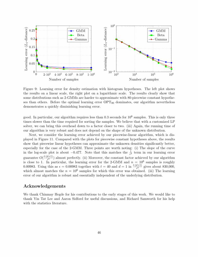
0 2·105 4·105 6·105 8·105 1·1060
0.05
0.1
0.15
0.2
0.25
Number of samples
Learning
error(L
1-distanc
e) GMMBeta
Gamma
103 104 105 10610−2
10−1
100
Number of samples
Learning
error(L
1-distanc
e) GMMBeta
Gamma
Figure 9: Learning error for density estimation with histogram hypotheses. The left plot showsthe results on a linear scale, the right plot on a logarithmic scale. The results clearly show thatsome distributions such as 2-GMMs are harder to approximate with 80-piecewise constant hypothe-ses than others. Before the optimal learning error OPT80 dominates, our algorithm neverthelessdemonstrates a quickly diminishing learning error.
good. In particular, our algorithm requires less than 0.3 seconds for 106 samples. This is only threetimes slower than the time required for sorting the samples. We believe that with a customized LPsolver, we can bring this overhead down to a factor closer to two. (iii) Again, the running time ofour algorithm is very robust and does not depend on the shape of the unknown distribution.
Next, we consider the learning error achieved by our piecewise-linear algorithm, which is dis-played in Figure 11. Compared with the plots for piecewise constant hypotheses above, the resultsshow that piecewise linear hypotheses can approximate the unknown densities significantly better,especially for the case of the 2-GMM. Three points are worth noting: (i) The slope of the curvein the log-scale plot is about −0.477. Note that this matches the 1
ε2term in our learning error
guarantee O( t·(d+1)ε2
) almost perfectly. (ii) Moreover, the constant factor achieved by our algorithmis close to 1. In particular, the learning error for the 2-GMM and n = 106 samples is roughly0.00983. Using this as ε = 0.00983 together with t = 40 and d = 1 in t·(d+1)
ε2gives about 830,000,
which almost matches the n = 106 samples for which this error was obtained. (iii) The learningerror of our algorithm is robust and essentially independent of the underlying distribution.
Acknowledgements
We thank Chinmay Hegde for his contributions to the early stages of this work. We would like tothank Yin Tat Lee and Aaron Sidford for useful discussions, and Richard Samworth for his helpwith the statistics literature.
46

0 2·105 4·105 6·105 8·105 1·106
0.05
0.1
0.15
0.2
0.25
Number of samples
Run
ning
time(secon
ds) GMM
BetaGamma
103 104 105 10610−2
10−1
100
Number of samples
Run
ning
time(secon
ds) GMM
BetaGamma
Figure 10: Running times for density estimation with piecewise-linear hypotheses. The left plotshows the results on a linear scale, the right plot on a logarithmic scale. As predicted by ouranalysis, the running time of our algorithm scales nearly-linearly with the input size n. Moreover,the constant in the big-O is quite small: for n = 106, our algorithm takes less than 0.3 seconds,which is only three times slower than sorting the samples. Note that this means that no algorithmthat relies on sorting the samples can be more than 4 times faster than our algorithm when thetotal running time with sorting is taken into account. As before, the running time of our algorithmis also essentially independent of the unknown distribution.
References
[ADH+15] J. Acharya, I. Diakonikolas, C. Hegde, J. Li, and L. Schmidt. Fast and Near-OptimalAlgorithms for Approximating Distributions by Histograms. In PODS, 2015.
[AK01] S. Arora and R. Kannan. Learning mixtures of arbitrary Gaussians. In STOC, pages247–257, 2001.
[AM05] D. Achlioptas and F. McSherry. On spectral learning of mixtures of distributions. InCOLT, pages 458–469, 2005.
[BB05] M. Bagnoli and T. Bergstrom. Log-concave probability and its applications. Economictheory, 26(2):445–469, 2005.
[BBBB72] R. E. Barlow, D. J. Bartholomew, J. M. Bremner, and H. D. Brunk. Statistical Inferenceunder Order Restrictions. Wiley, New York, 1972.
[BD14] F. Balabdaoui and C. R. Doss. Inference for a Mixture of Symmetric Distributionsunder Log-Concavity. Available at http://arxiv.org/abs/1411.4708, 2014.
[Bir87a] L. Birgé. Estimating a density under order restrictions: Nonasymptotic minimax risk.Annals of Statistics, 15(3):995–1012, 1987.
[Bir87b] L. Birgé. On the risk of histograms for estimating decreasing densities. Annals ofStatistics, 15(3):1013–1022, 1987.
47

0 2·105 4·105 6·105 8·105 1·1060
0.05
0.1
0.15
0.2
0.25
Number of samples
Learning
error(L
1-distance) GMM
BetaGamma
103 104 105 106
10−2
10−1
100
Number of samples
Learning
error(L
1-distanc
e) GMMBeta
Gamma
Figure 11: Learning error for density estimation with piecewise-linear hypotheses. The left plotshows the results on a linear scale, the right plot on a logarithmic scale. The slope of the curvein the log-scale plot is roughly −.477, which almost exactly matches the asymptotic guarantee forour algorithm. Moreover, the average learning error for 2-GMMs with n = 106 samples is about0.00983. Substituting this into the theoretical guarantee t·(d+1)
ε2gives a sample requirement of
roughly 830,000, i.e., very close to the 106 samples our algorithm required to achieve this error.Similar to the running time, the learning error is also robust and essentially independent of theunderlying distribution.
[Bru58] H. D. Brunk. On the estimation of parameters restricted by inequalities. The Annalsof Mathematical Statistics, 29(2):pp. 437–454, 1958.
[BRW09] F. Balabdaoui, K. Rufibach, and J. A. Wellner. Limit distribution theory for maximumlikelihood estimation of a log-concave density. The Annals of Statistics, 37(3):pp. 1299–1331, 2009.
[BS10] M. Belkin and K. Sinha. Polynomial learning of distribution families. In FOCS, pages103–112, 2010.
[BSZ15] A. Bhaskara, A. T. Suresh, and M. Zaghimoghaddam. Sparse Solutions to NonegativeLinear Systems and Applications. In AISTATS, 2015.
[BW07] F. Balabdaoui and J. A. Wellner. Estimation of a k-monotone density: Limit distributiontheory and the spline connection. The Annals of Statistics, 35(6):pp. 2536–2564, 2007.
[BW10] F. Balabdaoui and J. A. Wellner. Estimation of a k-monotone density: characterizations,consistency and minimax lower bounds. Statistica Neerlandica, 64(1):45–70, 2010.
[CDSS13] S. Chan, I. Diakonikolas, R. Servedio, and X. Sun. Learning mixtures of structureddistributions over discrete domains. In SODA, pages 1380–1394, 2013.
[CDSS14a] S. Chan, I. Diakonikolas, R. Servedio, and X. Sun. Efficient density estimation viapiecewise polynomial approximation. In STOC, pages 604–613, 2014.
48

[CDSS14b] S. Chan, I. Diakonikolas, R. Servedio, and X. Sun. Near-optimal density estimation innear-linear time using variable-width histograms. In NIPS, pages 1844–1852, 2014.
[Che82] E. W. Cheney. Introduction to Approximation Theory: Second Edition. AMS ChelseaPublishing, 1982.
[CS13] Y. Chen and R. J. Samworth. Smoothed log-concave maximum likelihood estimationwith applications. Statist. Sinica, 23:1373–1398, 2013.
[CSS10] M. Cule, R. Samworth, and M Stewart. Maximum likelihood estimation of a multi-dimensional log-concave density. Journal of the Royal Statistical Society: Series B(Statistical Methodology), 72:545–607, 2010.
[Csu04] M. Csuros. Maximum-scoring segment sets. IEEE/ACM Trans. Comput. Biol. Bioin-formatics, 1(4):139–150, October 2004.
[CT04] K. S. Chan and H. Tong. Testing for multimodality with dependent data. Biometrika,91(1):113–123, 2004.
[Das99] S. Dasgupta. Learning mixtures of Gaussians. In FOCS, pages 634–644, 1999.
[DDO+13] C. Daskalakis, I. Diakonikolas, R. O’Donnell, R.A. Servedio, and L. Tan. Learning Sumsof Independent Integer Random Variables. In FOCS, pages 217–226, 2013.
[DDS12a] C. Daskalakis, I. Diakonikolas, and R.A. Servedio. Learning k-modal distributions viatesting. In SODA, pages 1371–1385, 2012.
[DDS12b] C. Daskalakis, I. Diakonikolas, and R.A. Servedio. Learning Poisson Binomial Distribu-tions. In STOC, pages 709–728, 2012.
[DDS15] C. Daskalakis, I. Diakonikolas, and A. Stewart. Personal communication, 2015.
[DeV98] R. A. DeVore. Nonlinear approximation. ACTA NUMERICA, 7:51–150, 1998.
[DG85] L. Devroye and L. Györfi. Nonparametric Density Estimation: The L1 View. JohnWiley & Sons, 1985.
[DJ98] D. L. Donoho and I. M. Johnstone. Minimax estimation via wavelet shrinkage. Annalsof Statistics, 26(3):879–921, 1998.
[DJKP95] D. L. Donoho, I. M. Johnstone, G. Kerkyacharian, and D. Picard. Wavelet shrinkage:asymptopia. Journal of the Royal Statistical Society, Ser. B, pages 371–394, 1995.
[DJKP96] D. L. Donoho, I. M. Johnstone, G. Kerkyacharian, and D. Picard. Density estimationby wavelet thresholding. Annals of Statistics, 24(2):508–539, 1996.
[DK14] C. Daskalakis and G. Kamath. Faster and sample near-optimal algorithms for properlearning mixtures of gaussians. In COLT, pages 1183–1213, 2014.
[DK15] I. Diakonikolas and D. Kane. Personal communication, 2015.
49
[DL01] L. Devroye and G. Lugosi. Combinatorial methods in density estimation. Springer Seriesin Statistics, Springer, 2001.
[DR09] L. Dumbgen and K. Rufibach. Maximum likelihood estimation of a log-concave densityand its distribution function: Basic properties and uniform consistency. Bernoulli,15(1):40–68, 2009.
[DS00] S. Dasgupta and L. Schulman. A two-round variant of EM for Gaussian mixtures. InUAI, pages 143–151, 2000.
[DW13] C. R. Doss and J. A. Wellner. Global Rates of Convergence of the MLEs of Log-concaveand s-concave Densities. Available at http://arxiv.org/abs/1306.1438, 2013.
[FM99] Y. Freund and Y. Mansour. Estimating a mixture of two product distributions. InCOLT, pages 183–192, 1999.
[FOS05] J. Feldman, R. O’Donnell, and R. Servedio. Learning mixtures of product distributionsover discrete domains. In FOCS, pages 501–510, 2005.
[Fou97] A.-L. Fougères. Estimation de densités unimodales. Canadian Journal of Statistics,25:375–387, 1997.
[GJ14] P. Groeneboom and G. Jongbloed. Nonparametric Estimation under Shape Constraints:Estimators, Algorithms and Asymptotics. Cambridge University Press, 2014.
[Gre56] U. Grenander. On the theory of mortality measurement. Skandinavisk Aktuarietidskrift,39:125–153, 1956.
[Gro85] P. Groeneboom. Estimating a monotone density. In Proc. of the Berkeley Conferencein Honor of Jerzy Neyman and Jack Kiefer, pages 539–555, 1985.
[GW09] F. Gao and J. A. Wellner. On the rate of convergence of the maximum likelihoodestimator of a k-monotone density. Science in China Series A: Mathematics, 52:1525–1538, 2009.
[Hen88] P. Henrici. Applied and Computational Complex Analysis, Power Series IntegrationConformal Mapping Location of Zero. Applied and Computational Complex Analysis.Wiley, 1988.
[HP76] D. L. Hanson and G. Pledger. Consistency in concave regression. The Annals of Statis-tics, 4(6):pp. 1038–1050, 1976.
[HP15] M. Hardt and E. Price. Sharp bounds for learning a mixture of two gaussians. In STOC,2015.
[HW15] Q. Han and J. A. Wellner. Approximation and Estimation of s-Concave Densities viaRenyi Divergences. Available at http://arxiv.org/abs/1505.00379, 2015.
[Ize91] A. J. Izenman. Recent developments in nonparametric density estimation. Journal ofthe American Statistical Association, 86(413):205–224, 1991.
50
[JW09] H. K. Jankowski and J. A. Wellner. Estimation of a discrete monotone density. ElectronicJournal of Statistics, 3:1567–1605, 2009.
[Kha79] L. Khachiyan. A polynomial algorithm in linear programming. Soviet Math. Dokl,20:1093–1096, 1979.
[KL04] V. N. Konovalov and D. Leviatan. Free-knot splines approximation of s-monotonefunctions. Advances in Computational Mathematics, 20(4):347–366, 2004.
[KL07] V. N. Konovalov and D. Leviatan. Freeknot splines approximation of sobolev-typeclasses of s -monotone functions. Adv. Comput. Math., 27(2):211–236, 2007.
[KM10] R. Koenker and I. Mizera. Quasi-concave density estimation. Annals of Statistics,38(5):2998–3027, 2010.
[KMR+94] M. Kearns, Y. Mansour, D. Ron, R. Rubinfeld, R. Schapire, and L. Sellie. On thelearnability of discrete distributions. In STOC, pages 273–282, 1994.
[KMV10] A. T. Kalai, A. Moitra, and G. Valiant. Efficiently learning mixtures of two Gaussians.In STOC, pages 553–562, 2010.
[KP92] G. Kerkyacharian and D. Picard. Density estimation in Besov spaces. Statistics &Probability Letters, 13(1):15–24, 1992.
[KPT96] G. Kerkyacharian, D. Picard, and K. Tribouley. Lp adaptive density estimation.Bernoulli, 2(3):pp. 229–247, 1996.
[KS14] A. K. H. Kim and R. J. Samworth. Global rates of convergence in log-concave densityestimation. Available at http://arxiv.org/abs/1404.2298, 2014.
[KSV08] R. Kannan, H. Salmasian, and S. Vempala. The spectral method for general mixturemodels. SIAM J. Comput., 38(3):1141–1156, 2008.
[Las01] J. B. Lasserre. Global optimization with polynomials and the problem of moments.SIAM Journal on Optimization, 11(3):796–817, 2001.
[LB99] J. Q. Li and A. R. Barron. Mixture density estimation. In NIPS, pages 279–285, 1999.
[Lin95] B. Lindsay. Mixture models: theory, geometry and applications. Institute for Mathe-matical Statistics, 1995.
[LS14] Y. T. Lee and A. Sidford. Path finding methods for linear programming: Solving linearprograms in O
√rank iterations and faster algorithms for maximum flow. In FOCS,
pages 424–433, 2014.
[LS15] J. Li and L. Schmidt. A Nearly Optimal and Agnostic Algorithm for Properly Learninga Mixture of k Gaussians, for any Constant k. Manuscript, available on arxiv., 2015.
[Mar92] VA Markov. On functions deviating least from zero in a given interval. Izdat. Imp.Akad. Nauk, St. Petersburg, pages 218–258, 1892.
51

[MV10] A. Moitra and G. Valiant. Settling the polynomial learnability of mixtures of Gaussians.In FOCS, pages 93–102, 2010.
[Pan01] V. Y. Pan. Univariate polynomials: nearly optimal algorithms for factorization androotfinding. In ISSAC, pages 253–267. ACM, 2001.
[Par03] P. A. Parrilo. Semidefinite programming relaxations for semialgebraic problems. Math-ematical programming, 96(2):293–320, 2003.
[Pea95] K. Pearson. Contributions to the mathematical theory of evolution. ii. skew variation inhomogeneous material. Philosophical Trans. of the Royal Society of London, 186:343–414, 1895.
[Rao69] B. L. S. Prakasa Rao. Estimation of a unimodal density. Sankhya A, 31:23–36, 1969.
[RW84] R. A. Redner and H. F. Walker. Mixture densities, maximum likelihood and the EMalgorithm. SIAM Review, 26:195–202, 1984.
[Sco92] D. W. Scott. Multivariate Density Estimation: Theory, Practice and Visualization.Wiley, New York, 1992.
[SHKT97] C. J. Stone, M. H. Hansen, C. Kooperberg, and Y. K. Truong. Polynomial splines andtheir tensor products in extended linear modeling: 1994 wald memorial lecture. Annalsof Statistics, 25(4):1371–1470, 1997.
[Sho87] N. Z. Shor. Class of global minimum bounds of polynomial functions. Cybernetics andSystems Analysis, 23(6):731–734, 1987.
[Sil86] B. W. Silverman. Density Estimation. Chapman and Hall, London, 1986.
[SOAJ14] A. T. Suresh, A. Orlitsky, J. Acharya, and A. Jafarpour. Near-optimal-sample estimatorsfor spherical gaussian mixtures. In NIPS, pages 1395–1403, 2014.
[Sto94] C. J. Stone. The use of polynomial splines and their tensor products in multivariatefunction estimation. Annals of Statistics, 22(1):pp. 118–171, 1994.
[Tim63] A. F. Timan. Theory of approximation of functions of a real variable, volume 34. CourierCorporation, 1963.
[TSM85] D. M. Titterington, A. F. M. Smith, and U. E. Makov. Statistical analysis of finitemixture distributions. Wiley & Sons, 1985.
[Vai89] P. Vaidya. A new algorithm for minimizing convex functions over convex sets. In FOCS,pages 338–343, 1989.
[Vai96] P. M. Vaidya. A new algorithm for minimizing convex functions over convex sets.Mathematical Programming, 73(3):291–341, 1996.
[Val84] L. G. Valiant. A theory of the learnable. In STOC, pages 436–445. ACM Press, 1984.
52

[VC71] V. Vapnik and A. Chervonenkis. On the uniform convergence of relative frequenciesof events to their probabilities. Theory of Probability and Its Applications, 16:264–280,1971.
[VW02] S. Vempala and G. Wang. A spectral algorithm for learning mixtures of distributions.In FOCS, pages 113–122, 2002.
[VZGG13] J. Von Zur Gathen and J. Gerhard. Modern computer algebra. Cambridge universitypress, 2013.
[Wal09] G. Walther. Inference and modeling with log-concave distributions. Statistical Science,24(3):319–327, 2009.
[Weg70] E. J. Wegman. Maximum likelihood estimation of a unimodal density. I. and II. Annalsof Mathematical Statistics, 41:457–471, 2169–2174, 1970.
[WN07] R. Willett and R. D. Nowak. Multiscale poisson intensity and density estimation. IEEETransactions on Information Theory, 53(9):3171–3187, 2007.
[WW83] E. J. Wegman and I. W. Wright. Splines in statistics. Journal of the American StatisticalAssociation, 78(382):pp. 351–365, 1983.
Appendix
A Analysis of the General Merging Algorithm: Proof of Theo-rem 17
This section is dedicated to the proof of Theorem 17. The proof is a generalization of that ofTheorem 10. Recall the statement of Theorem 17:
Theorem 17. Let Op and Oc be η-approximate Ak-projection and Ak-computation oracles forD. Algorithm General-Merging(f, t, α, ε, δ) draws n = O((αdt + log 1/δ)/ε2) samples, runs intime O
((Rp(n) +Rc(n)) log n
αt
), and outputs a hypothesis h and an interval partition I such that
|I| ≤ 2α · t and with probability at least 1− δ, we have
‖h− f‖1 ≤ 3 ·OPTD,t +OPTD,t + ε
α− 1+ 2ε+ η . (10)
Proof. We first bound the running time. The number of iterations of the algorithm is O(log(n/αt))by the same argument as for histograms, since the number of intervals reduces by a factor of 3/4 ineach iteration. In each iteration, we compute the closest function in D and the corresponding Ad+1
distance, hence the runtime per iteration is bounded by Rp(n) +Rc(n), by definition.We now prove the error guarantee. Let I = I1, . . . , It′ be the partition of I returned by
General-Merging, and let h be the function returned. The desired bound on t′ is immediatesince the algorithm terminates only when t′ ≤ 2αt. We now prove (10).
Let h∗ ∈ Dt be such that ‖h∗ − f‖1 = OPTD,t. Let I∗ = I∗1 , . . . , I∗t be a partition withat most t pieces such that h∗ ∈ DI∗i for all i. Call the end-points of I∗j ’s as jumps of h∗. For
53

any interval J ⊆ I let Γ(J) be the number of jumps of h∗ in the interior of J . Since we drawn = Ω((αdt+ log 1/δ)/ε2) samples, Corollary 4 implies that with probability at least 1− δ,
‖f − f‖A(2α+1)(d+1)t≤ ε .
We condition on this event throughout the analysis.We split the total error into three terms based on the final partition I:
Case 1: Let F be the set of intervals in I with no jumps in h∗, i.e., F = J ∈ I |Γ(J) = 0.
Case 2a: Let J0 be the set of intervals in I that were created in the initial partitioning step of thealgorithm and contain a jump of h∗, i.e., J0 = J ∈ I | Γ(J) > 0 and J ∈ I0.
Case 2b: Let J1 be the set of intervals in I that contain at least one jump, and were created bymerging two other intervals, i.e., J1 = J ∈ I | Γ(J) > 0 and J /∈ I0.
Notice that F ,J0,J1 form a partition of I, and thus
‖h− f‖1 = ‖h− f‖1,F + ‖h− f‖1,J0 + ‖h− f‖1,J1 .
We bound the error from above in the three cases separately. In particular, we will show:
‖h− f‖1,F ≤ 3 · ‖f − h∗‖1,F + 2 · ‖f − f‖A|F|·(d+1),F +η
2αt|F| , (14)
‖h− f‖1,J0 ≤ ‖f − f‖A|J0|·(m+1),J0 , (15)
‖h− f‖1,J1 ≤OPTD,t + ε
(α− 1)+ ‖f − f‖Ad·t+|J1|,J1 + ‖f − h∗‖1,J1 +
η
2(α− 1). (16)
Using these results along with the fact that ‖f − h∗‖1,F + ‖f − h∗‖1,J1 ≤ OPTD,t and α > 2, wehave
‖h− f‖1 ≤ 3 ·OPTD,t +OPTD,t + ε
α− 1+ 2‖f − f‖A|F|(d+1)
+ ‖f − f‖A|J0|d
+ ‖f − f‖A(|J1|+t)d+
η
2αt(|F|+ J1)
(a)
≤ 3 ·OPTD,t +OPTD,t + ε
α− 1+ 2‖f − f‖A2αt(d+1)
+ η
(b)
≤ 3 ·OPTD,t +OPTD,t + ε
α− 1+ 2ε+ η ,
where (a) follows from Fact 6(d) and since (|F| + |J1| + |J0|) ≤ 2αt, and (b) follows from the VCinequality. Thus, it suffices to prove Equations (14)–(16).
Case 1. We first consider the set of intervals in F . By the triangle inequality we have
‖h− f‖1,F ≤ ‖f − h∗‖1,F + ‖h− h∗‖1,F .
For any interval J ∈ F , since h and h∗ are both in D, they have at most d sign changes, and
‖h− h∗‖1,J = ‖h− h∗‖Ad+1,J ≤ ‖h− f‖Ad+1,J + ‖f − h∗‖Ad+1,J .
54

By the definition of h and the projection oracle,
‖h− f‖Ad+1,J ≤ minh′∈DJ
‖h′ − f‖Ad+1,J +η
2αt≤ ‖h∗ − f‖Ad+1,J +
η
2αt.
Therefore,‖h− h∗‖1,J ≤ 2 · ‖h∗ − f‖Ad+1,J +
η
2αt.
Again by the triangle inequality,
‖h∗ − f‖Ad+1,J ≤ ‖h∗ − f‖Ad+1,J + ‖f − f‖Ad+1,J .
Summing over the intervals in F ,∑J∈F‖h∗ − f‖Ad+1,J ≤
∑J∈F‖h∗ − f‖Ad+1,J +
∑J∈F‖f − f‖Ad+1,J
≤ ‖h∗ − f‖1,F + ‖f − f‖A|F|(d+1),F
Combining these, we obtain,
‖h− f‖1,F ≤ 3 · ‖f − h∗‖1,F + 2 · ‖f − f‖A|F|(d+1),F +η
2αt|F| ,
which is precisely (14).
Case 2a. We now analyze the error for the intervals J0. The set I0 contains only singletons andintervals with no sample points. By definition, with probability 1, only the intervals in I0 thatcontain no samples may contain a jump of h∗. The singleton intervals containing the sample pointsdo not include jumps, and are hence covered by Case 1. Since J0 does not contain any samples, ouralgorithm assigns
h(J) = f(J) = 0
for any J ∈ J0. Hence,‖h− f‖1,J0
= ‖f‖1,J0,
and
‖h− f‖1,J0= ‖f‖1,J0
=∑J∈J0
|f(J)|
=∑J∈J0
|f(J)− f(J)|
≤ ‖f − f‖A|J0|(d+1),J0,
where the last step simply follows from non-negativity of f − f over J0.
55

Case 2b. We finally consider J1, the set of intervals created by merging in some iteration of ouralgorithm that also contain jumps. As before, our first step is the following triangle inequality:
‖h− f‖1,J1 ≤ ‖h− h∗‖1,J1 + ‖h∗ − f‖1,J1 .
Consider an interval J ∈ J1 with Γ(J) ≥ 1 jumps of h∗. Since h ∈ DJ , h − h∗ has at mostd · Γ(J) sign changes in J . Therefore,
‖h− h∗‖1,J(a)= ‖h− h∗‖Ad·Γ(J)+1,J
(b)
≤ ‖h− f‖Ad·Γ(J)+1,J + ‖f − f‖Ad·Γ(J)+1,J + ‖f − h∗‖Ad·Γ(J)+1,J
(c)
≤ Γ(J)‖h− f‖Ad+1,J + ‖f − f‖Ad·Γ(J)+1,J + ‖f − h∗‖1,J , (17)
where (a) follows from Fact 6(a), (b) is the triangle inequality, and inequality (c) uses Fact 6(c)along with the fact that Γ(J) ≥ 1 and d ≥ 1. We start by bounding the Ad+1 distance in the firstterm above.
Lemma 49. For any J ∈ J1, we have
‖h− f‖Ad+1,J ≤OPTD,t + ε
(α− 1)t+
η
2(α− 1)t. (18)
Before proving this lemma, we use it to complete Case 2b. Summing (7) over J ∈ J1 andplugging in the lemma,
‖h− h∗‖1,J1 ≤
∑J∈J1
(Γ(J)
· (OPTD,t + ε
(α− 1)t+
η
2(α− 1)t
)+∑J∈J1
‖f − f‖Ad·Γ(J)+1,J + ‖f − h∗‖1,J1
(a)
≤OPTD,t + ε
(α− 1)+
η
2(α− 1)+ ‖f − f‖Ad·t+|J1|,J1 + ‖f − h∗‖1,J1
where the first term in (a) uses the fact that∑
J∈J1Γ(J) ≤ t and the second term uses this in
conjunction with Fact 6(d).We now prove Lemma 49.
Proof of Lemma 49. Each iteration of our algorithm merges pairs of intervals except those with theαt largest errors. Therefore, if two intervals were merged, there were at least αt other interval pairswith larger error. We will use this fact to bound the error on the intervals in J1.
Suppose an interval J ∈ J1 was created in the jth iteration of the while loop of our algorithm,i.e., J = I ′i,j+1 = I2i−1,j ∪ I2i,j for some i ∈ 1, . . . , sj/2. Recall that the intervals I ′i,j+1, fori ∈ 1, . . . , sj/2, are the candidates for merging at iteration j. Let h′ be the distribution givenby applying the projection oracle to the empirical distribution over each candidate interval I ′j+1 =I ′1,j+1, . . . , I
′sj/2,j+1. Note that h′(x) = h(x) for x ∈ J since J remains intact through the
remainder of the algorithm.As with the histogram estimation, for a class D with at most d sign changes, let ed(g, J) =
ming′∈DJ ‖g− g′‖Ad+1. Let L be the set of candidate intervals I ′i,j+1 in the set I ′j+1 with the largest
α · t errors ‖h′ − f‖Ad+1. By the guarantee of projection oracle,
‖h′ − f‖Ad+1,I′i,j+1≤ ed(f , I ′i,j+1) +
η
2αt.
56

Let L0 be the intervals in L that do not contain any jumps of h∗. Since h∗ has at most t jumps,|L0| ≥ (α− 1)t.
Therefore, ∑I′∈L0
‖h′ − f‖Ad+1,I′ ≤∑I′∈L0
(ed(f , I
′) +η
2αt
)≤∑I′∈L0
(‖h∗ − f‖Ad+1,I′ +
η
2αt
)≤ ‖f − h∗‖1,L0 + ‖f − f‖A(d+1)αt,L0 + η/2
≤ OPTD,t + ε+ η/2.
Since h′ is h on the interval J , combining with |L0| ≥ (α− 1)t, we obtain
‖h′ − f‖Ad+1,J= ‖h− f‖Ad+1,J
≤OPTD,t + 2ε
(α− 1)t+
η
2(α− 1)t,
completing the proof of the lemma.
B Additional Omitted Proofs
B.1 Proof of Fact 26
We first require the following classical lemma, first proved by Markov [Mar92]. For completeness,we include an elegant proof by the mathoverflow user fedja7. We remark that the bounds in thefollowing fact are essentially tight.
Fact 50 ([Mar92]). Let p(x) =∑d
j=0 cjxj be a degree-d polynomial so that |p(x)| ≤ 1 for all
x ∈ [−1, 1]. Then maxj |cj | ≤ (√
2 + 1)d for all j = 0, . . . , d.
Proof. We first claim that |cj | ≤ maxz∈D |p(z)| where D is the unit complex disc. To see this, wenotice that by Cauchy’s integral formula,
cj =1
j!p(j)(0) =
1
2πi
∫|ζ|=1
p(ζ)
ζj+1dζ ,
where we also changed the order of differentiation and integration and used
d
dxjp(ζ)
ζ − x=
j! · p(ζ)
(ζ − x)j+1.
7See http://mathoverflow.net/questions/97769/approximation-theory-reference-for-a-bounded-polynomial-having-bounded-coefficie
57
Therefore, we get
|cj | =1
2π
∣∣∣∣∣∫|ζ|=1
p(ζ)
ζj+1dζ
∣∣∣∣∣≤ 1
2π
∫|ζ|=1
∣∣∣∣ p(ζ)
ζj+1
∣∣∣∣ dζ≤ max|ζ|=1
|p(z)| .
Consider the function
F (z) = z−mp
(z + z−1
2
).
On the domain z : |z| ≥ 1, this function is analytic. So by the maximum modulus principle, it isbounded by its value on the unit circle. Since for all z ∈ D, (z + z−1)/2 = <(z), we conclude that|F (z)| ≤ maxx∈[−1,1] p(x) ≤ 1 by assumption. Thus we have that
p
(z + z−1
2
)≤ zd
for all |z| > 1. Fix any w ∈ D. It is straightforward to see that w = (z+z−1)/2 for some z ∈ C\0;by symmetry of z and z−1 we conclude that this also holds for some z with |z| ≥ 1. For each w,arbitrarily choose such a z and denote it zw. Moreover, for all |z| > (
√2 + 1), we have∣∣∣∣z + z−1
2
∣∣∣∣ ≥ |z| − |z−1|2
>
√2 + 1− 1√
2+1
2≥ 1
and thus we conclude that for all w ∈ D we have that its corresponding zw satisfies |zw| ≤√
2 + 1and therefore |p(w)| = |p((zw + z−1
w )/2)| ≤ zdw ≤ (√
2 + 1)d, as claimed.
The above statement is for polynomials that are uniformly bounded on [−1, 1]. We will beinterested in bounds for polynomials that integrate to a fixed constant. In order to relate thesebounds, we use the following classical result.
Fact 51 (Bernstein’s Inequality [Che82]). Let p be a degree-d polynomial and let p′ be its derivative.Then
maxx∈[−1,1]
|p′(x)| ≤ d2 · maxx∈[−1,1]
|p(x)| .
With these results, we are now ready to prove Lemma 26.
Proof of Lemma 26. Consider the degree-(d + 1) polynomial P such that P (−1) = 0 and P ′ = p.This implies that P (x) =
∫ x−1 p(y) dy. Since p is non-negative on [−1, 1], the bound on
∫ 1−1 p(y) dy
then givesmax
x∈[−1,1]|P (x)| ≤ α · (
√2 + 1)d .
Using Bernstein’s Inequality (Fact 51), we can convert this bound into a bound on P ′ = p, i.e., weget that |p(x)| ≤ t · (d + 1) for all x ∈ [−1, 1]. Combining this uniform bound on p with Fact 50gives the desired bound on the coefficients of p.
58

B.2 Proof of Lemma 34
Our approach to proving Lemma 34 is relatively straightforward. Assume we had an algorithm Athat finds the roots of p exactly. Then one could perform a non-negativity test by running A to findthe roots of p′, which correspond to the extrema of p. Given the extrema of p, it suffices to checkwhether p is non-negative at those points and the endpoints of the interval.
However, such an exact root-finding algorithm A does not exist in general. Nevertheless, thereare efficient algorithms for finding the approximate roots of p in certain regimes. We leverage theseresults to construct an efficient non-negativity test. Before we proceed, we remark briefly thatwe could also utilize the univariate SOS algorithm [Sho87, Las01, Par03], which is arguably moreelementary than our approach here, but slower.
Formally, we build on the following result.
Fact 52 ([Pan01], Part II, Theorem 1.1). Let D denote the complex unit disc. For all ν > 0,there exists an algorithm FindRoots(q, β) satisfying the following guarantee: given any degree-dpolynomial q(z) : C → C with roots z1 . . . , zd such that zi ∈ D for all i and β ≥ d log d, returnsz∗1 , . . . , z
∗d so that |z∗j − zj | ≤ 22−β/d for all j. Moreover, FindRoots runs in time O(d log2 d ·
(log2 d+ log β)).
Our polynomials do not necessarily have all roots within the complex unit disc. Moreover, we areonly interested in real roots. However, it is not too hard to solve our problems with the algorithmfrom Fact 52. We require the following structural result:
Fact 53 ([Hen88], Sect. 6.4). Let q(x) = xd + cd−1xd−1 + . . .+ c1x+ c0 be a monic polynomial of
degree d (i.e., the leading coefficient is 1). Let ρ(q) denote the norm of the largest zero of q. Then
ρ(q) ≤ 2 max1≤i≤d
|cd−i|1/i .
In order to use the result above, we process our polynomial p so that it becomes monic and stillhas bounded coefficients. We achieve this by removing the leading terms of p with small coefficients.This then allows us to divide by the leading coefficient while increasing the other coefficients by acontrolled amount only. Formally, we require the following definitions.
Definition 54 (Truncated polynomials). For any degree-d polynomial p =∑d
i=0 cixi and ν > 0 let
∆ = ∆(p, ν) = maxi : |ci| ≥
ν
2d
,
and let Π = Πν be the operator defined by
(Πp)(x) =
∆(p,ν)∑i=0
cixi.
Formally, Π acts on the formal coefficient representation of p as q =∑cix
i. It then returns aformal representation
∑∆(p,ν)i=0 cix
i. In a slight abuse of notation, we do not distinguish between theformal coefficient representation of p and the polynomial itself. Then Facts 52 and 53 give us thefollowing:
59

Lemma 55. There exists an algorithm FastApproxRoots(p, ν, µ) with the following guarantee.Let p be a polynomial as in Definition 34, and let ν, µ > 0 such that ν ≤ 1
2αd (where α and d are asin Def. 34). Then FastApproxRoots returns approximate roots x∗1, . . . , x
∗∆(p,ν) ∈ R so that for
all real roots y of Πνp, there is some j so that |y − x∗j | ≤ µ. Moreover, FastApproxRoots runsin time O(d log2 d · (log2 d+ log logα+ log log(1/ν) + log log(1/µ))).
Proof. FastApproxRoots(p, ν, µ) proceeds as follows. We find ∆ = ∆(p, ν) and Πp = Πνp intime O(d) by a single scan through the coefficients ci of p. Let q1(x) = 1
c∆(Πp)(x). Note that the
roots of q1 are exactly the roots of Πp. Then, by Theorem 53, we have that
Adef= 2 max
1≤i≤∆
∣∣∣∣c∆−ic∆
∣∣∣∣1/i ≥ ρ(q1) .
The quantity A is also simple to compute in a single scan of the ci. Notice that we have
A ≤ max
(2 max
1≤i≤∆
∣∣∣∣c∆−ic∆
∣∣∣∣ , 1) ≤ 2αd
ν︸︷︷︸B
by the definition of ∆ and the assumption that the ci are bounded by α (Definition 34). Let Bdenote the right hand side of the expression above. If we let q(x) = q1(Ax), we have that the rootsof q all lie within the complex unit disc. Let z1, . . . , z∆ be the roots of Πp. Then the roots of q areexactly z1/A, . . . , z∆/A. Run FindRoots(q, 2d + d logB + d log(1/µ)), which gives us z∗1 , . . . , z∗∆so that for all i, we have |z∗i − zi/A| < µ/B. Thus, for all i, we have
|Az∗i − z| ≤ Aµ
B≤ µ .
FastApproxRoots(p, ν, µ) returns the numbers x∗i = <(Az∗i ). For any real root x of Πp, thereis some z∗i so that |Az∗i − x| < µ, and thus |x∗i − x| < µ as well. Thus, we output numbers whichsatisfy the conditions of the Lemma. Moreover, the runtime of the algorithm is dominated by theruntime of FindRoots(q, 2d+ d logB + d log(1/µ)), which runs in time
O(d log2 d · (log2 d+ log(d logB + d log(1/µ)))) =
O(d log2 d · (log2 d+ log logα+ log log(1/ν) + log log(1/µ)))
This completes the proof.
Proof of Lemma 34. Let ν = µ2 , and let ν ′ = µ
4αd(d+1) . Set
r = (Πνp)(x) =
∆(p,ν)∑i=1
cixi .
We can compute the coefficients of r in time O(d). Moreover, Π(r′(x)) = r′(x). Let x1, . . . , xd′ ,where d′ ≤ ∆, be the roots of r′(x) in [−1, 1]. These points are exactly the local extrema of r on[−1, 1]. Our algorithm TestNonneg(p, µ) then is simple:
1. Run FastApproxRoots(r, ν ′, µ) and let x∗1, . . . , x∗∆ be its output.
60

2. Let J = i : x∗i ∈ [−1, 1] and construct the set S = −1, 1 ∪ xi : i ∈ J.
3. Denote the points in S by x0 = −1 ≤ x1 ≤ . . . ≤ xd′−1 ≤ xd′ = 1, where d′ ≤ ∆ + 1.
4. Evaluate the polynomial p at the points in S using the fast algorithm from Fact 41.
5. If at any of these points the polynomial evaluates to a negative number, return that point.Otherwise, return “OK”.
The running time is dominated by the call to FastApproxRoots. By Lemma 55, this algorithmruns in time O(d log2 d · (log2 d+ log logα+ log log(1/µ))) as claimed.
It suffices to prove the correctness of our algorithm. Clearly, if p is nonnegative on [−1, 1], itwill always return “OK”. Suppose there exists a point y ∈ I so that p(y) < −µ.
For a function f , and an interval I = [a, b], let |f |∞,I = supx∈I ‖f(x)‖. Then,
‖p− r‖∞,[−1,1] ≤ supx∈[−1,1]
∣∣∣∣∣d∑
i=∆+1
cixi
∣∣∣∣∣ (a)
≤ (d−∆) · µ4d≤ µ/4 , (19)
where the inequality (a) follows from the choice of ∆. Thus r(y) < −3µ/4. Since the pointsx0, x1, . . . , xd′ are extremal for r on I, there exists a 0 ≤ j ≤ d′ so that r(xj) < −3ν/4. If j = 0(resp. j = m′), so if r(−1) < −3µ/4 (resp. r(1) < −3µ/4), then by Equation (19), we havep(−1) < µ/2 (resp. p(1) < −µ/2). Thus our algorithm correctly detects this, and the polynomialfails the non-negativity test as intended.
Thus assume j ∈ 1, . . . ,∆. By Lemma 55, we know that there is a x∗` so that |x∗` − xj | < ν ′.Since xj ∈ I, either ` ∈ J or |xj + 1| < ν ′ or |xj − 1| < ν ′, so in particular, there is a point s ∈ S sothat |xj − s| < ν ′. Since for all x ∈ [−1, 1], we have
|p′(x)| ≤d∑i=1
∣∣icixi∣∣ ≤ αd(d+ 1)
by the bound on the coefficients of p (see Definition 34). By a first order approximation, we havethat
|p(xj)− p(s)| ≤ αd(d+ 1)|xj − s| ≤ µ/4
where the last inequality follows by the definition of ν ′. Thus, we have that p(s) < −µ/2, and wewill either return s or some other point in s′ ∈ S with p(s′) ≤ p(s). Thus our algorithm satisfiesthe conditions on the theorem.
C Learning discrete piecewise polynomials
Throughout this paper we focused on the case that the unknown distribution has a density fsupported on [−1, 1], and that the error metric is the L1-distance with respect to the Lebesguemeasure on the real line. We now show that our algorithm and analysis naturally generalize to thecase of discrete distributions.
In the discrete setting, the unknown distribution is supported on the set [N ]def= 1, . . . , N, and
the goal is to minimize the `1-distance between the corresponding probability mass functions. The
61
`1-norm of a function f : [N ]→ R is defined to be ‖f‖1 =∑N
i=1 |f(i)| and the `1-distance betweenf, g : [N ]→ R is ‖f − g‖1.
In the following subsections, we argue that our algorithm also applies to the discrete settingwith only minor adaptations. That is, we can agnostically learn discrete piecewise polynomialdistributions with the same sample complexity and running time as in the continuous setting.
C.1 Problem statement in the discrete setting
Fix an interval I ⊆ [N ]. We say that a function p : I → R is a degree-d polynomial if there is adegree-d real polynomial q : R → R such that p(i) = q(i) for all i ∈ I. We say that h : [N ] → R isa t-piecewise degree-d polynomial if there exists a partition of [N ] into t intervals so that on eachinterval, h is a degree-d polynomial. Let Pdisc
t,d be the set of t-piecewise degree-d polynomials on [N ]which are nonnegative at every point in [N ]. Fix a distribution (with probability mass function)f : [N ] → R. As in the continuous setting, define OPTdisc
t,ddef= ming∈Pdisc
t,d‖g − f‖1 . As before, our
goal is the following: given access to n i.i.d. samples from f , to compute a hypothesis h so thatprobability at least 9/10 over the samples, we have ‖h− f‖1 ≤ C ·OPTdisc
t,d + ε , for some universalconstant C. As before, we let f denote the empirical after taking n samples.
Our algorithms for the continuous setting also work for discrete distributions, albeit with slightmodifications. For the case of histogram approximation, the algorithm and its analysis hold verbatimfor the discrete setting. The only difference is in the definition of flattening; Definition 8 applies tocontinuous functions. For a function f : [N ]→ R and an interval J ⊆ [n] the flattening of f on J isnow defined to be the constant function on J which divides the total `1 mass of the function withinJ uniformly among all the points in J . Formally, if J = a, . . . , b, we define the flattening of f onJ to be the constant function fJ(x) =
∑i∈I f(i)
b−a+1 .
C.2 The algorithm in the discrete setting
Our algorithm in the discrete setting is nearly identical to the algorithm in the continuous setting,and the analysis is very similar as well. Here, we only present the high-level ideas of the dis-crete algorithm and highlight the modifications necessary to move from a continuous to a discretedistribution.
C.2.1 The Ak-norm and general merging in the discrete setting
We start by noting that the notion of the Ak-norm and the VC inequality also hold in the discretesetting. In particular, the Ak-norm of a function f : [N ]→ R is defined as
‖f‖Ak = maxI1,...,Ik
k∑i=1
|f(Ii)| ,
where the maximum ranges over all I1, . . . , Ik which are disjoint sub-intervals of [N ].The basic properties of the Ak-norm (i.e., those in Lemma 6) still hold true. Moreover, it is
well-known that the VC inequality (Theorem 2) still holds in this setting. These properties of theAk-norm are the only ones that we use in the analysis of GeneralMerging. Therefore, it is readilyverified that the same algorithm is still correct, and has the same guarantees in the discrete setting,assuming appropriate approximate Ak-projection and Ak-computation oracles for polynomials ona fixed subinterval of [N ].
62

C.2.2 Efficient Ak-projection and computation oracles for polynomials
We argue that, as in the continuous setting, we can give efficient Ak-projection and computationoracles for non-negative polynomials of degree d on a discrete interval I, using an O(d)-dimensionalconvex program. By appropriately shifting the interval, we may assume without loss of generalitythat the interval is of the form [m] = 1, . . . ,m for some m ≤ N .
The Convex Program As in the continuous case, it can be shown that the set of non-negativepolynomials p on [m] satisfying ‖p− f‖Ak ≤ τ is convex (as in Lemma 21), for any fixed τ > 0 (since‖ · ‖Ak is a norm). Moreover, using explicit interpolation formulas for polynomials on [m], it is easyto show that every polynomial in this feasible region has a representation with bounded coefficients(the analogue of Theorem 27), and that the feasible region is robust to small perturbations in thecoefficients (the analogue of Theorem 28). Thus, it suffices to give an efficient separation oracle forthe feasible set.
The Separation Oracle Recall that the separation oracle in the continuous case consisted of twocomponents: (i) a non-negativity checker (Subsection 6.2), and (ii) a fast Ak-computation oracle(Subsection 6.3). We still use the same approach for the discrete setting.
To check that a polynomial p : I → R with bounded coefficients is non-negative on the points inI, we proceed as follows: we use Fast-Approx-Roots to find all the real roots of p up to precision1/4, then evaluate p on all the points in I which have constant distance to any approximate root ofp. Since p cannot change sign in an interval without roots, this is guaranteed to find a point in Iat which p is negative, if one exists. Moreover, since p has at most d roots, we evaluate p at O(d)points; using Fact 41, this can be done in time O(d log d log log d).
Finally, to compute the Ak-distance between p =∑d
j=0 cjxj and f on an interval I, we use the
same reduction as in Section 6.3 with minor modifications. The main difference is that between twopoints xi, xi+1 in the support of the empirical distribution, the quantity p[xi, xi+1] (see section 6.3)is now defined to be
p[xi, xi+1] =
xi+1−1∑`=xi+1
p(`)
=
xi+1−1∑`=xi+1
d∑j=0
cj`j
=d∑j=0
cj
xi+1−1∑`=xi+1
`j
.
Notice that the above is still a linear expression in the cj , and there are simple closed-form expres-sions for
(∑β`=α `
j)for all integers α, β and for all 0 ≤ j ≤ d. Following the arguments in Section
6.3 with this substituted quantity, one can show that the quantity returned by ApproxSepOraclein the discrete setting is still a separating hyperplane for p and the current feasible set. Moreover,ApproxSepOracle still runs in time O(d).
63