1

Discovering the defects in paintings using non-destructive testing (NDT) techniques and passing through measurements of deformation

S. Sfarra1a, C. Ibarra-Castanedob, D. Ambrosinia, D. Paolettia, A. Bendadab, X. Maldagueb

aLas.E.R. Laboratory, University of L’Aquila, Department of Industrial and Information Engineering and Economics (DIIIE), Piazzale E. Pontieri 1, Loc. Monteluco di Roio, Roio Poggio, L’Aquila

(AQ), Italy I-67100; bComputer Vision and Systems Laboratory, Laval University, Department of Electrical and Computer Engineering, 1065 av. de la Médecine, Quebec City, Québec (QC), Canada,

G1V 0A6

ABSTRACT

The present study is focused on two topics. The former is a mathematical model useful to understand the deformation of paintings, which uses straining devices, adjustable and micrometrically controlled through a pin implanted in a hollow cylinder. Strains were analyzed by holographic interferometry (HI) technique using an appropriate frame. The latter concerns the need to improve the conservator’s knowledge about the defect’s detection and defect’s propagation in acrylic painting characterized by underdrawings and pentimenti. To accomplish this task, a sample was manufactured to clarify the several uncertainties inherent the influence of external factors on their conservation. Subsurface anomalies were also retrieved by near-infrared reflectography (NIRR) and transmittography (NIRT) techniques, using LED lamps and several narrow-band filters mounted on a CMOS camera, working at different wavelengths and in combination with UV imaging. In addition, a sponge glued on the rear side of the canvas was impregnated with a precise amount of water by means of a syringe to verify the stretcher effect by digital speckle photography (DSP) technique (using MatPIV). The same effect also affects the sharp transition of the canvas at the stretcher’s edge. In this case, the direct mechanical contact between stretcher and canvas was investigated by HI technique. Finally, advanced algorithms were successfully applied to the square pulse thermography (SPT) data to detect three Mylar® inserts simulating different types of defects. These fabricated defects were also identified by optical techniques: DSP and laser speckle imaging (LSI). Keywords: square pulse thermography; holographic interferometry; digital speckle photography; paintings; defects; deformations

1. INTRODUCTION In the last thirty years, specific attention has been reserved to the preservation of canvas paintings. Great progress in understanding how a canvas painting is manufactured and how it responds to its environment and strain’s actions have been made. Conservators began to understand that not only the canvas and sizing but also the paint could respond to moisture very significantly. Moreover, the moisture content influences the mechanical properties of the paint, making it more susceptible to the effects of heat and pressure [1]. Degradation process in art objects is usually slow and gradual. Although this situation is preferable from a curator’s point of view, it represent a problem for conservation scientists who would like to clarify the mechanism responsible for these degradation process. In the absence of direct information on the behaviour over time, local spatial differences in the condition of a material within a single object can provide important clues to factors that enhance or reduce degradation. These local differences are therefore of special interest in the conservation science. In the field of the conservation of canvas paintings, an example of such local difference is the variation between the condition of the paint layer and that of the canvas in the regions directly over the stretcher, strainer or cross bars and the condition of the painting in the other regions behind which no wood is present. The term stretcher is used to indicate any part of the wooden support of the canvas, and refers to the local, sharp transition in the condition of the painted canvas. It is known as stretcher effect. Although this effect is well-known to paintings conservators, the explanations of why it happens is a matter of current research. The most popular explanation

1 stefano.sfarra@univaq.it; phone ++39 (0) 862 434362; fax ++39 (0) 862 431233.

2

for this effect is that the presence of the stretcher induces a local deviation of the relative humidity behind the canvas, which controls the moisture content of the canvas, ground, and paint layers [2]. This local deviation of the moisture content leads to a locally distinct swelling of the layers in the painting at the stretcher area in comparison to the area where no stretcher is present. Over time this might lead to the stretcher effect [3]. Paintings elaborated with acrylic artist paints seem indestructible even to the latter effect, compared to many more delicate painting mediums such as gouache, watercolor, encaustics and tempera, or drawing mediums such as pastels or charcoal. Under several environmental conditions, acrylic paintings are very flexible, and this dramatically reduces the potential of cracking in most situations. The price paid for this flexibility is a softer film; one that can be scratched, scuffed and marred easily. Another property of this flexible paint surface is the relative permeable nature of the waterborne acrylic. This property allows to the dirt or pollutants to become embedded (especially in a fresher film). Finally, the most significant property of the acrylic film (again especially representative of fresh films) is the potential tackiness of the surface. With this information it is possible to say that canvas is the core of a painting, since it is strictly linked to mechanical stress induced by environmental local variations [4]. Lining canvas is a complex material and to perform a decent selection process it might be important to know its map of deformations and the stress-distribution under several boundary conditions and different loads, as well as its dynamic response in ambient drift. At present, it is not possible to study in laboratory all the parameters at the same time; the mechanical response of a sample subject to a particular kind of loading ought to be performed in a controlled environment. The first topic of this work explores the possibility of applying a displacement derivative measurement utilizing the double-exposure (DE) holographic interferometry (HI) for the inspection of a canvas model treated with glue, under different condition of load, in order to determine the strain-stress distribution; these parameters are of interest since they affect the lifetime of the structure [5]. The second topic is focused on the painted sample, which represents a detail of La crocifissione di San Sepolcro (beginning of XVI century), by Luca Signorelli, i.e., the part where an author’s pentimento was detected. Also the underdrawings were reproduced as showed in the real case and inspected by near-infrared reflectography (NIRR) and transmittography (NIRT) techniques [6], as well as by UV imaging [7]. A CMOS camera (Canon 40DH 22.2 x 14.8 mm – 10 megapixel 0.38-1.0 μm) and narrow-band filters were used for the acquisition of the UV, NIR reflectography/transmittography, and DE-HI data. In addition, three defects in Mylar® with different thickness were inserted at different depths. The canvas affected by biological attack was also repaired in several parts to simulate previous restorations. Since this type of artworks show a great sensibility to humidity changes, which cause deformations due to shrinkage and swelling, a sponge fixed on the rear side of the canvas was impregnated with water and inspected during the drying process using digital speckle photography (DSP) technique (MatPIV manual) [8].Visual inspection was the only technique capable of retrieving the positions of fungal attack affecting the canvas on the rear side. According to a previous experiment, which used the TV-Holography technique, the real-time deformations occurred during the humidity changes may be caused by the ground layer movements, while the upper colour layer(s) is relatively unchangeable [9]. In addition, the real behaviour of paintings where the stretcher is at close contact with the canvas, and where the latter provides direct mechanical support, was studied by HI technique [5]. The Mylar® inserts, simulating occurring detachments between the canvas and the paint layers, and/or inclusions of foreign materials inside the canvas layer, were analyzed by square pulse thermography (SPT) and detected applying advanced algorithms to the infrared thermography data [10], as well as to the optical techniques (DSP and LSI). Finally, the Kubelka-Munk theory explains why the author’s pentimento and his signature are not identifiable and why this is not happening in the real case [11].

2. NON-DESTRUCTIVE TESTING (NDT) METHODSIn this chapter, the paper is organized into 6 sections (from 2.1. to 2.6.) to provide the Readers with a relevant theoretical background about the sensing techniques used. The data processing techniques used for each of these methods are also described into 5 subsections (2.1.1.; 2.2.1.; 2.3.1.; 2.6.1.; 2.6.2). In addition, in Table 1 are reported all the fundamental technical information, as well as the pros and cons of the various NDT methods used in this work.

NDTmethods

Holographic Interferometry

Speckle Digital reflected-ultraviolet imaging

Near-InfraRed Reflectography and Transmittography

Infrared Thermography

Processing Laser Speckle Pulsed Phase

3

technique or mode of image

acquisition

Double-Exposure Imaging UV band-pass filter: 360 nm

IR band-pass filter: 680 nm

ThermographyParticle Image Velocimetry

Principal Component

ThermographyType of the

methodOptical Thermal

Type of the stress applied

Blow dryer Halogen lamp: 250 W

UV illuminator: 360 nm

Halogen lamp: 250 W

IR lamps: 125 WLEDs lamp: 940 nm

[working without the IR BP filter]

Detector array number of elements

>3000 lines/mm [holographic plate]

3888 x 2592 pixels [camera]

3888 x 2592 pixels [camera]

3888 x 2592 pixels [camera]

320 x 240 pixels[camera]

3888 x 2592 pixels [camera]

Cost of the equipment

Medium-High Medium-High Medium Medium Medium-High

In-situ operation Very poor Good Very good Very good GoodSensitivity High Medium High High Medium-High

Main advantages Different types of defects can be detected; shallow defects can be easily detected

This method allows the conservator to

examine the condition of the

varnish layer and may also detect fungal growth

The details hidden to the direct sight, gives

precious indications both on

the realization technique and on

the state of conservation of the

artwork to restorers and art historians and, in some cases, it can help of the artwork

authenticity

Large surface areas of materials can be inspected rapidly and at low cost in

term of implementation of the measurements; part with complex

geometry are routinely inspected

Main disadvantages

The detection of deeper defects depends on the material under inspection

Very old over-paintings or retouching

executed in the past and examined with the UV light can be

difficult to distinguish as they tend to fluoresce

after hundred years.

Some types of paints can mask

subsurface defects

The processing of a large amount of data can be time

consuming

Tab. 1 Fundamental technical information (yellow background with dotted lines), advantage and disadvantage (green background with solid lines) of the NDT methods used

2.1 Holographic Interferometry (HI)

Holographic interferometry (HI) is a non-destructive full-field technique that measures small static or sinusoidal deformations occurring in a object, based upon standard holographic principles [12]. Holography is a method for recording three-dimensional information on a two-dimensional recording medium (photographic emulsion, thermoplastics, etc.). Unlike a photograph, the hologram (“Holo” – whole, “Gram” – message) contains all the information about the surface of the object and the effects of parallax. The hologram is an interference pattern of coherent wavefronts scattered from the object and recorded by the medium. To create a hologram, a coherent light source is split into an object beam and a reference beam. The object beam illuminates the object and then is reflected onto the holographic recording medium.

4

The reference beam follows a path that is nominally identical in length to the object beam, but illuminates the medium directly. Any difference in path length that occurs between the two beams is due to the surface contours of the object. Therefore, the incident light on the medium from the two beams is out of phase. This phase difference creates an interference pattern that can be recorded. In the case of photographic emulsion on a glass plate as the medium, re-illumination of the processed plate with a replica of the reference beam causes the interference pattern to be reconstructed. An apparent complete reproduction of the object is then visible through the holographic plate [13]. In conventional interferometry, an object wavefront is combined with a reference wavefront to create an interference pattern at the detector which allows for an understanding of the variations in the object wavefront. Combining conventional interferometry with holography, it is possible produce three-dimensional interferograms images of diffusively-reflecting, three dimensional objects that are overlaid with interference fringes indicating areas of deformation or displacement in the object. Similarly, transparent objects will be overlaid with fringes indicating a change in refractive index of the material as due to a structural deformity or change in thickness. Such interferometry is possible because the light field scattered from an object may be first holographically recorded, then holographically reconstructed and compared to another light field scattered from the same object under different conditions, all with interferometric precision. In this type of interferometry, called HI, at least one of the waves is holographically reconstructed. The combination of two or more waves (of which one is a hologram) is referred to as a holographic interferogram (whereas a simple interference pattern recorded on a flat screen in intensity – as by the eye – is referred to simply as an interferogram, no modifier).There are several flavors of holographic interferometry, but most rely on a similar basic principle: the combination of (1) a reference hologram recorded while the object is in neutral equilibrium, with no stress applied, and (2) a second image or holographic image created while the captured is being subjected to some form of stress, i.e., mechanical, thermal, vibrational, etc [14]. In some cases, even a single hologram may be sufficient for the purposes of holographically interferometry. In addition to the advantages of the full-field nature of the measurement and the high sensitivity, the method does not require any special surface preparation, so that it can be applied to any structural surface, even to non-optical surfaces, such as those of composite materials [15]. In displacement measurements by holographic interferometry, the commonly used technique is DE-HI.

2.1.1 Double-Exposure (DE) Holographic Interferometry (HI) technique

In DE-HI, both the reference hologram and subject hologram are recorded in the same photographic plate. Upon development, the plate will then be illuminated using the reference beam, and the resulting hologram observed will consist of a three-dimensional image of the original object, overlaid with a pattern of interference fringes. Notably, the arrangement of the fringes will change as the viewing angle shifts, in similar fashion to the viewing of a single hologram. To understand the origin of the fringes, the two fields that are recreated using the double-exposure hologram are subsequently written. The first field – the field of the object captured in the reference hologram – is written as:

U0 (x , y )=a ( x , y )exp [− jφ ( x , y ) ] (1)

The second field – that of the stressed object captured in the subject hologram – is affected primarily by a phase change due to the deformation:

U'0 (x , y )=a ( x , y )exp {− j [φ ( x , y )+Δφ ( x , y ) ] } (2)

The observed intensity of the reconstructed wave is given by:

I ( x , y )=|U0 (x , y )+U0' ( x , y )|2=|a ( x , y ) exp [− jφ (x , y ) ]+a ( x , y ) exp {− j [φ ( x , y )+ Δφ ( x , y ) ] }|2

=

¿2 a2 ( x , y ) {1+cos [ Δφ ( x , y ) ]}(3)

The fact that the fields (and not intensities) of the two object waves add is the crux of the holographic interferometry, it is what makes interferometry by holography superior to classical interferometry, particularly when investigating three dimensional effects.It is the linearity of the holographic process that gives rise to the phenomenon of field addition. As Eq. 3 shows, the observed intensity will consist of the intensity of the original object modulated by the fringe pattern {1+cos[Δϕ(x,y)]}. Dark fringes indicate the specific positions where the subject hologram and reference hologram are perfectly out of phase (that is, Δϕ is an odd-integer multiple of π), and light fringes are the positions where the subject and reference

5

holograms constructively interfere (Δϕ is an even-integer multiple of π). Moving from one fringe to another corresponds to an out-of-plane displacement of the object that is equal to half the wavelength of the illuminating light. The location and density of these fringes may be easily related to physical qualities of the object under study.It is clear that the mentioned method is useful for the inspection of artworks if the subsurface anomalies induce detectable perturbations in the deformation of the surface. Usually, the stressing technique is chosen empirically with guidance provided by simple analysis of the anticipated deformation and by previous results obtained from programmed models. However, the presence of a temperature gradient between the layers of the sample linked to a difference in thermal conductivity of the various materials used for their fabrication is sufficient to create an appreciable local deformation in the anomaly area [16]. Usually, the thermal drift, i.e., heating the upper layer of a sample by using a stream of moderately warm air (with surface temperature rising up of maximum 3 °C in respect to the ambient temperature), and the ambient drift, i.e., working under room parameters variation, are the main stressing techniques exploited during an HI inspection [17].

2.2 Physics of speckles

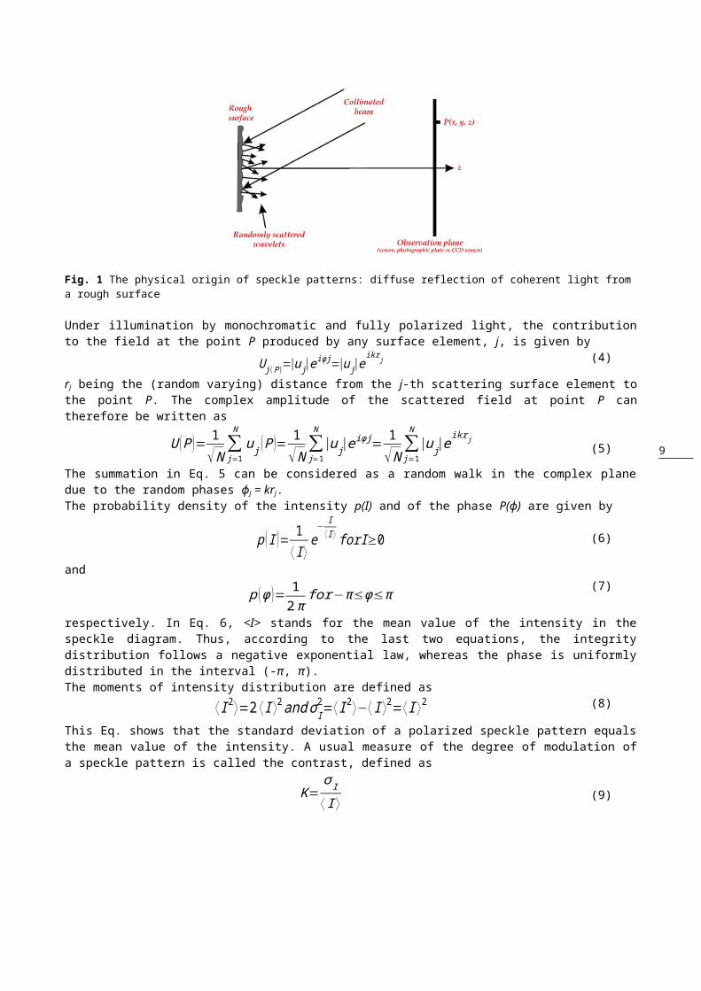
When an image obtained starting from a rough surface illuminated by a coherent light (e.g. a laser beam), a speckle pattern is observed in the image plane; this is called “subjective speckle pattern”, or simply “image speckle”. It is called “subjective” because the detailed structure of the speckle pattern depends on the viewing system parameters; for instance, if the size of the lens aperture changes, the size of the speckles change. If the position of the imaging system is altered, the pattern will gradually change and will eventually be unrelated to the original speckle pattern.When laser light which has been scattered off a rough surface falls on another surface, it forms an “objective speckle pattern”. If a photographic plate or another 2-D optical sensor is located within the scattered light field without a lens, a speckle pattern is obtained whose characteristics depend on the geometry of the system and the wavelength of the laser. Objective speckles are usually obtained in the far-field and called “far field speckles”. Speckles can be observed also close to the scattering object, in the near field. This kind of speckles are called “near field speckles”. Rigorously, a speckle pattern is a random intensity pattern produced by the mutual interference of a set of wavefronts. In optics and physics, a wavefront is the locus (a line, or, in a wave propagating in three dimensions, a surface) of points having the same phase. Thus the phenomenon can be observed with different media such as radio waves, or coherent light as in lasers.Assuming ideal conditions for producing a speckle pattern – single-frequency laser light and a perfectly diffusing surface with a Gaussian distribution of surface height fluctuations – it can be shown that the standard deviation of the intensity variations in the speckle pattern is equal to the mean intensity. In practice, speckle patterns often have a standard deviation that is less than the mean intensity, and this is observed as a reduction in the contrast of the speckle pattern. Indeed, it is usual to define the speckle contrast as the ratio of the standard deviation to the mean intensity.No matter which picture is assumed, it is easily realized that the light field at a specific point P(x,y,z) in a speckle pattern must be the sum of a large number N of components representing the contribution from all points on the scattering surface (Figure 1) [18-20].

Fig. 1 The physical origin of speckle patterns: diffuse reflection of coherent light from a rough surface

6

Under illumination by monochromatic and fully polarized light, the contribution to the field at the point P produced by any surface element, j, is given by

U j(P )=|u j|eiφj=|u j|e

ikr j (4)

rj being the (random varying) distance from the j-th scattering surface element to the point P. The complex amplitude of the scattered field at point P can therefore be written as

U ( P )= 1√N ∑

j=1

N

u j ( P )= 1√N ∑

j=1

N

|u j|eiφj= 1

√ N ∑j=1

N

|u j|eikr j (5)

The summation in Eq. 5 can be considered as a random walk in the complex plane due to the random phases ϕj = krj.The probability density of the intensity p(I) and of the phase P(ϕ) are given by

p ( I )= 1⟨ I ⟩

e−

I⟨ I ⟩ forI≥0 (6)

and

p (φ )= 12 π

for−π≤φ≤π(7)

respectively. In Eq. 6, <I> stands for the mean value of the intensity in the speckle diagram. Thus, according to the last two equations, the integrity distribution follows a negative exponential law, whereas the phase is uniformly distributed in the interval (-π, π).The moments of intensity distribution are defined as

⟨ I 2 ⟩=2⟨ I ⟩2 and σ I2=⟨ I 2⟩−⟨ I ⟩2=⟨ I ⟩2 (8)

This Eq. shows that the standard deviation of a polarized speckle pattern equals the mean value of the intensity. A usual measure of the degree of modulation of a speckle pattern is called the contrast, defined as

K=σ I

⟨ I ⟩(9)

This information, together with the result in Eq. 8 means that the contrast of a polarized speckle pattern is always unity, and the speckle pattern is said to be fully developed. In practice, the pattern is not fully developed and

K=σI

⟨ I ⟩≤1 (10)

2.2.1 Laser Speckle Imaging (LSI) technique

Figure 2 shows a diagram of the experimental setup.

Fig. 2 Schematic diagram of LSI experimental setup

7

A He-Ne laser (CRISEL INSTRUMENT S.r.l.) provided polarized, coherent light at 532 nm wavelength. The laser outputs a maximal power of 250 mW as measured with a power meter equipped with an integrating sphere detector. Rotating a linear polarized in the laser path provided control over beam intensity. The laser beam size was expanded to illuminate a 15 cm painting area at 45° incidence. In order to compare laser speckle image with incoherent imaging, a 250 W lamp was used to provide a uniform diffuse light. Painting was placed on the flat surface of an optical table. Light returning from the target was captured at normal incidence by a CMOS camera (EOS 40DH, CANON). A fixed aperture of f/11 was used throughout the experiment. Within a lens assembly a 532 nm filter was used to reject ambient light and assure comparison of equivalent wavelengths when the broadband incoherent light source was used. A sequence of images was acquired with fixed exposure time and interval (one image each five seconds). The images were digitized and processed by a computer.Because the LSI technique can be considered as an innovative approach in the cultural heritage field, below are reported the main points that characterize the method.The temporal speckle contrast image was constructed by calculating the ratio of standard deviation and mean value of each image pixel in the time sequence. The value of pixel (i, j) in the speckle contrast image was calculated as:

C i , j=√ 1

N−1 ∑t=t0

T

( X i , jt −X̄ i , j)

2

X̄ i , j

(11)

where the numerator is the standard deviation of the sequence and the denominator is the mean value of the sequence. Xt

i,j is the (i, j) pixel of the image acquired at time t; N is the total number of images acquired in the sequence; t0 is the time that the first image in the sequence was acquired; and T is the time that the last image in the sequence was acquired.

The time interval ΔT between two consecutive images was fixed in the experiments. X̄ i , j is the mean value of pixel (I,

j) in the time image averaged speckle image:

X̄ i , j=1N ∑

t=t0

T

X i , jt (12)

The temporal speckle statistics in the form of Eq. 11 is analogous to the classical concept of speckle contrast, which is defined in spatial domain and applied to calculate the spatial characteristics of a speckle pattern [21].In practice, by adjusting the capture parameters (e.g., exposure time, incident power, and time interval between subsequent capture), LSI is able to reveal structures that are hidden under the surface. Surface and subsurface lack of homogeneities depend differently on these capture parameters, so by tuning the capture parameters, the image contrast values of the surface and subsurface targets can be changed. When the contrast of the surface lack of homogeneity is within the noise level of the background image, the surface effect is essentially removed from the image [22-25].

2.3 Digital Speckle Photography (DSP)

Speckle photography is based on recording of objective or subjective speckle patterns, before and after the object is subjected to load. This is one of the simplest method in which a laser-lit diffuse surface is recorded at two different states of stress [26]. Speckle photography allows to measure in-plane displacements and derivatives of deformation. Speckle photography is exploited for metrology by using either a photographic plate or a CCD detector as the recording medium. In this case, it is called digital speckle photography (DSP).An expanded laser beam illuminates the object that scatters light. This technique starts with a picture before loading (reference image) and then a series of pictures are taken during the deformation process (deformed images). All the deformed images show a different random dot pattern relative to the initial non-deformed reference image. With computer software these differences between patterns can be calculated by correlating all the pixels of the reference image and any deformed image, and a strain distribution map can be created (Figure 3). In the present case, the particle image velocimetry (PIV) technique linked to MatPIV manual software was used [27].

8

Fig. 3 The image before deformation shows four dots of different shapes of gray that represents four different pixels. The image after deformation shows the same four dots, but now representing other four pixels. The computer software calculates the difference between dots location (pixels) of the different images and correlates them to determine the deformation

2.3.1 Particle Image Velocimetry (PIV) technique

The PIV technique is a correlation method. Correlation of two functions f(x) and g(x) is defined as the integral of the product of f*(x) with g(x), the latter shifter over some distance Δx

f⋅g=C fg ( Δx )=∫−∞

+∞

f ¿ (x ) g ( x+ Δx ) dx (13)

The superscript asterisk means that the complex conjugated value is taken. As we are dealing with real signals, the asterisk is irrelevant here. So far each shift Δx the correlation is calculated. This means that if a structure moves as a whole, besides random and offset correlations, a correlation maximum will be found at the shift corresponding to the translation. For example, two delta functions are reported

f ( x )=δ (x−x f ) ,g ( x )=δ ( x−xg ).

(14)

Then the correlation isC fg ( Δx )=δ ( x−x fg ) (15)

withx fg=xg−x f (16)

The correlation shows a peak at xfg. It is zero elsewhere. This situation is illustrated in Figure 4.

Fig. 4 Example of cross-correlation with two Dirac-functions

Suppose that the correlation of two discretized functions must be calculated and the number of points of each function is equal to N. Then the value of the correlation involves N2 operations. If this is performed in a two-dimensional plane of

9

two N x N collocation points, then the number of operations increases to N4. This number of operations easily becomes very large. This is the reason why Fourier theory is employed to evaluate correlations [28].In cross-correlation mode each particle is illuminated only once in each sample. Therefore, a pair of successive images is required in order to evaluate the cross-correlation. There is no self-correlation and since the order of the images is known there is no directional ambiguity. The disadvantage of cross-correlation is the necessity to acquire two images in a very short time interval. With the presently available lasers and CCD cameras this is no problem anymore. Furthermore, the spatial resolution is higher if compared to the auto-correlation mode. This is due to the larger information contents of an image pair, in contrast to a single image.

2.4 Digital reflected-ultraviolet (UV) imaging

UV radiation has shorter wavelengths than visible light. The natural source of UV radiation is the sun but it can also be emitted by specially designed fluorescent lamps, mercury vapour lamps and light-emitting diodes. All these artificial ultraviolet sources emit the UV radiation at different wavelength. The most useful UV band in the examination of artworks is 360 nm (near UV). Today almost any painting analysis begin with UV examination because it is a very quick and inexpensive test that can provide very useful information and help to determine what would be the next approximate analysis technique or conservation approach.Digital reflected-ultraviolet imaging has been for a long time a specialized area of imaging technology that has only found its way into a rather limited number of applications, in spite of the fact that film-based reflected-UV photography has been around for over a century. This is due in part to the characteristics of electronic imaging devices: CCDs and CMOS arrays generally have a greatly reduced sensitivity to UV light relative to visible and near-infrared. It is critical that these undesirable wavebands be removed to get pure reflected-UV images, while still preserving the UV sensitivity of the system. There is also a great deal of confusion about the difference between reflected-UV imaging and UV-fluorescence imaging. Many people think that the term “UV imaging” refers to the latter. Instead, reflected-UV and UV-fluorescence imaging are different techniques that see different things in a scene.UV-fluorescence imaging starts with a UV excitation source that stimulates fluorescence of a material, that is, the re-emission of light at a longer wavelength. The fluorescence signal is often visible light that can be imaged with a conventional camera.In contrast, reflected-UV imaging begins with a UV light source, and ends with the imaging of reflected UV light at the same wavelength by a special UV camera. In the past, this type of photography was done with standard black-and-white film, which sees UV light quite well. Unfortunately, this method suffers from serious limitations related to composition, exposure control and focus. These limitations stem from the visible-light opacity of the UV pass filter combined with the inability of the eye to see UV light through the viewfinder, as well as the fact that light meters (whether external or in cameras) are not designed to measure UV light levels. These difficulties, combined with a dearth of widely-available information about the proper techniques, have prevented film-based UV imaging from becoming as widespread as it might have otherwise.Digital reflected-UV imaging overcomes all of the limitations of film (albeit with a lower resolution for the time being).The UV spectrum is divided into various sub-bands, with the most common convention dividing the region of the spectrum between 250 and 400 nm (the near-UV band) into the A, B and C bands. In this convention, the A band is between 360 and 400 nm, the B between 320 and 360 nm, and the C between 250 and 320 nm. UV below 250 nm is sometimes called the deep-UV band. Below 100 nm, UV light is heavily absorbed by air, and experiments done in this band must be conducted in vacuo.As interest in digital reflected-UV imaging has grown, a small number of camera manufacturers and lens designers have specifically addressed the demands of this market and have produced off-the-shelf UV cameras based on silicon CCDs. UV sensitivity is often overlooked by CCD and CMOS camera manufacturers, who usually publish spectral response curves for their sensors that stop short at 400 nm, the edge of human vision and the beginning of the near-UV region of the spectrum. Most of the emerging breed of UV-specific cameras are based on thinned CCD arrays. The thinning process removes silicon material that prevents UV radiation from reaching the active layer in the detectors. This thinning process shortens the cut-on wavelength of the sensor down as low as ~200 nm.UV illumination is often quite weak in indoor situations, requiring that active illumination to be used. Traditional UV sources include both high and low pressure mercury discharge lamps which generate UV light at 365 nm and 254 nm respectively. These UV light sources are not pure ultraviolet in nature, since the lamp’s spectrum is broadband, and the colored-glass filters used to reduce visible and infrared light tend to leak red light, to which silicon detectors are quite

10

sensitive. A number of manufacturers are producing LEDs in the 365-400 nm waveband. These LEDs are typically very spectrally pure, with FWHM values of ~10 nm and have power levels up to 100 mW.In practice, in reflected UV photography the surface of the painting layer is illuminated directly by UV emitting lamps (radiation sources). The radiation is partly absorbed and reflected by the painting layer. A UV transmitting, visible light blocking filter is placed on the camera lens that allows only reflected ultraviolet to pass. The filter absorbs all visible light (Figure 5) [29-31].

Fig. 5 Schematic diagram of reflected UV photography experimental setup

2.5 Near-infrared reflectography (NIRR) and transmittography (NIRT)

Van Asperen de Boer first developed infrared reflectography in the 1960's using a lead-sulfide detector, which had a peak response of 2 microns. Although van Asperen de Boer initially used a Barnes T-4 infrared camera in his research, he soon switched to an infrared vidicon television system as soon as they became available. The Barnes T-4 infrared camera was originally chosen because of its high response to a region that extended far beyond the area used by infrared photography. Although satisfactory results were achieved, the Barnes camera also offered several disadvantages, including difficult mirror optics design, heavy and cumbersome instruments, difficulties in analyzing large paintings, and a high cost. The infrared vidicon television system helped to solve these problems [11].Infrared reflectography using a vidicon tube system soon became the preferred method to perform infrared analysis. Vidicon systems typically have a sensitivity that reaches about 2.0 mm. It was determined that the 1.5 - 2.0 mm region best reveals underdrawings done in chalk, charcoal, metals and inks [32]. In a vidicon tube system, a television camera is fitted with a vidicon tube, which is sensitive to infrared radiation. This is directly connected to a digital image processing system and the resultant image is displayed on a monitor. The same lamps used for infrared photography can be used to illuminate the imaged area. Filters can be placed in front of the imaged area to remove the visible radiation in order to reduce the resolution of the vidicon tube system [33]. The use of a filter becomes necessary as the thickness of a paint layer increases [34]. However, problems existed with the infrared vidicon television system. The vidicon tube is highly sensitive and can easily be damaged by over-exposure. Also, as the tube causes thermal noise as it heats up, and the system can only be operated for periods of about an hour at a time [34].An infrared reflectography system using a silicon CCD camera was first developed in the 1990's and is still currently used. Solid state CCD systems can range in sensitivity (typically anywhere in the range of 0.6 to 5.7 mm). A solid state CCD system are better than the vidicon tube system in terms of geometric distortion, signal stability, linearity and MTF. All of these characteristics improve the overall image quality [35]. Solid state CCD systems are also superior to vidicon tube systems in regards to sensitivity. This is most likely due to a CCD's high light sensitivity, low noise and high contrast that exists at any resolution [36]. Since a video system is restricted to 640x480 pixels, sampling areas of the painting and piecing them together into a "mosaic" will obtain the best results. Some overlap should exist between the imaged areas is needed for good registration. Twenty percent has proved to be a sufficient amount of overlap to recognize similar features while still keeping the number of images to a minimum [35]. Unfortunately, this need for a "mosaic of images" created difficulties. Because edges can appear within the result, there is a need for near-uniform illumination of the image space.To eliminate the need for a "mosaic", Bertani's research modified the infrared reflectography technique by making use of a scanning method. The infrared detector used in Bertani's procedure was a simple optical head placed at the center of

11

the image. A pinhole with a diameter of 0.4 mm was then placed in front of the detector so an object area of 0.2 mm could be sampled when the optical magnification was 2:1. A translation system was then used to move the optical head and a small illuminator along the X-Y plane. A personal computer made use of a 12-bit analog-to-digital converter to sample and digitize the output signal of the detector. An image-processing board then displayed the final result [37]. The use of a scanner removed the need for a "mosaic" and the result was a smoother image that requires less manipulation. It was also found that the image exhibited greater definition and legibility by using the infrared scanning method [37]. Infrared reflectography is able to solve some of the problems found in infrared photography. The greatest advantage is the increased sensitivity of infrared reflectography systems over infrared photography systems. Therefore, while an underdrawing will still remain hidden under most blue areas of a painting, the underdrawing is now visible in all green areas of the painting. Other advantages of infrared reflectography over infrared photography include speed and the ease of use. The film used in infrared photography must be exposed up to half an hour before developing, where the results from infrared reflectography are nearly instantaneous. Another drawback to infrared photography is photographs and film will deteriorate with age. However, the final result in infrared reflectography is digital, and as a result images captured using this method will not degrade over time. Also, details can be manipulated and enhanced using infrared reflectography. Overall, an infrared reflectography system is less expensive than one for infrared photography [34]. Despite improvements have been occurred, there are still limitations to the infrared reflectography method. The most difficult of these problems is that this method is still unable to penetrate blue areas of the painting. A related problem is that this method is unable to expose parts of an underdrawing covered by a medium that absorbs and reflects infrared radiation. The use of filters requires the illumination level of the imaged area to be increased. It is necessary for the X-Y translation of the object on a plane that is perpendicular to the camera. Images can still appear grayish and may therefore have poor contrast. Optical and geometrical distortions can be caused by the camera and must therefore be taken into account by the software when analyzing the data. However, the interpolation utilized by the software to correct these problems can also create errors and artifacts in the resulting image [37]. An understanding of the optical theory of Kubelka-Munk is necessary to determine the interaction of paint with light, or more specifically for this case the differences between the interaction of paint with visible radiation versus the interaction of paint with infrared radiation. The light flux incident on a paint layer is partly absorbed and partly scattered. The flux that is neither absorbed nor scattered by the surface of the paint is able to penetrate the paint layer. Diffusion of the light is created by the initial scattering and the re-scattering of the penetrating flux [11]. Internal reflectance exists when the diffuse flux is reflected by the ground and then by the under-side of the paint layer (Figure 6) [34].

Fig. 6 Interaction of light with paint layer and ground

The exact fractions of the light that are scattered and absorbed are defined by the coefficients S and K, respectively. Both of these coefficients are directly dependent on the thickness of the paint layer, which is defined by the variable X. The absorption coefficient and the scattering coefficient also vary with regards to the pigments used in a paint. The difference between the absorption coefficient and the scattering coefficient can be found by the equation

12

KS

=(1−R0 )2

2⋅R0

(17)

If a paint layer has a black background, it can be considered to be perfectly absorbing. Therefore, the reflectance of this layer of paint with a finite thickness is found to be a function of the scattering coefficient

S⋅X=b−1⋅coth( 1−a⋅R0

b⋅R0) (18)

where a and b are defined by the equations [38]

a=12⋅( R0

−1+R0)

b=12⋅( R0

−1−R0)(19)

Unfortunately, this ideally simplified equation does not usually exist for most situations. However, by using Kubelka's work varying absorption can be considered when determining the reflectance of a uniform paint layer (R) of a certain thickness (X) through the use of the following formula

R=1−RG⋅[a−b⋅coth (b⋅S⋅X ) ]

a−RG+b⋅coth (b⋅S⋅X )(20)

where a and b are defined by the equations

a=S+ KS

b=√a2−1(21)

Where RG is the ground reflectance, S is the scattering coefficient of the paint layer and K is the absorption coefficient [34]. Therefore, the successfulness of exposing the underdrawing is most affected by the scattering power of the paint layer and the thickness of the paint layer. The ability to extract the underdrawing is also affected by the contrast of both layers. As the wavelength of the radiation increases, the scattering by the particles is reduced. Therefore, at a longer wavelength, the radiation is able to pass through the layers of paint to be reflected or absorbed by the underdrawing, and the infrared radiation is capable of passing through the paint layer while visible radiation is reflected by it. The limitations of wavelength exist in the thermal IR, at about 5.0 mm [32]. There are some limitations that exist in the Kubelka-Munk theory. Since the theory assumes that Lambert's law is true, the specular reflectance from the upper side of the film boundary is not considered. This in turn means that the theory would be applicable only if the pigments are contained in a medium with the same index of refraction as the surrounding medium [11]. However, since it is only necessary to find an approximation of the relationship of the paint layer thickness to the radiation wavelength, Lambert's law is unimportant [39]. Another assumption is that there is uniformity of the scattering and absorption coefficients throughout the paint layer, which rarely occurs in older paintings. The absorption coefficient and scattering coefficient are both related to the pigment/medium ratio, or pigment volume concentration. For many paintings, pigments were hand ground and were therefore not uniform in size [11]. Again, however, various influences such as the refractive indices of the media and the need for uniformity of particle size can be disregarded because the relationship between thickness and wavelength must only be approximated [39], [40]. Another limitation of the Kubelka-Munk theory is that its parameters are dependent on wavelength [11].When an underdrawing exists, the background of a paint layer will have two distinctly different reflectances, RB

(background reflectance of the underdrawing) and RW (background reflectance of the ground). As the paint layer reflectance is dependent on the background reflectance, the paint layer will also exhibit two distinctly different reflectances. The contrast-ratio between these two paint layer reflectances is therefore found to be

13

k=RpB

R pG

(22)

Where RpB is the paint layer reflectance of the underdrawing and RpG is the paint layer reflectance of the ground. To obtain a certain contrast-ratio the layer thickness must equal the value XD. The contrast-ratio can then be found using the equation

k=RpB

R pG=

1−RB⋅[a−b⋅coth (b⋅S⋅X D ) ]1−RG⋅[a−b⋅coth (b⋅S⋅XD )]

⋅a−RG+b⋅coth (b⋅S⋅XD )a−RB+b⋅coth (b⋅S⋅X D )

(23)

The value XD is known as the hiding thickness. Therefore, an imaging system is able to differentiate between the background reflectance of the underdrawing and the background reflectance of the ground when the paint layer thickness is less than the hiding thickness [11]. To obtain a representation of the underdrawing of a painting, the above equation must be taken into consideration for the background reflectance of the underdrawing (RB). On the other hand, the image coming from the NIRT technique is collected by illuminating the back of the canvas with an incandescent lamp and capturing the transmitted radiation with a camera only sensitive to infrared wavelengths. Low energy NIRT photons transmit through many materials, but not through paints containing carbonaceous pigments, like charcoal or graphite. This imaging technique is often utilized to look through painted layers to identify the cartoon or sketch done by the artist prior to applying paints. These underdrawing, which were used to plan out the composition, were often executed in charcoal or pencil and hence show up in dark contrast on the NIRT image. Infrared imaging can also reveal abandoned or overpainted pictures that have used black pigments [41].

2.6 Infrared thermography (IRT)

A general definition of infrared thermography is: a diagnostic technique in which an infrared camera is used to measure temperature variations on the surface of the body, producing images that reveal sites of abnormal tissue growth; while, a technical definition suitable in the present case is: a non-destructive imaging technique that allows the inspection of different materials based on their surface temperatures. Within an appropriate thermal analysis, moisture and other structural damages can be detected [42].In this study, the specimen surface is stimulated with a heat square pulse (SP) and the cooling down process is recorded with an infrared camera for several minutes. The acquired data is then processed to improve defect contrast and signal-to-noise ratio. The method is called square pulse thermography (SPT) [43]. Several processing techniques exist, from a basic cold image subtraction to more advance techniques such as principal components or higher order statistics. The more relevant to the present study are described below.

2.6.1 Pulse Phase Thermography (PPT) technique

In the PPT method, an individual rectangular heat pulse is used and the characteristic thermal response of the object to this pulse is analyzed. The heat response signal can be presented as a superimposition of the number of waves, each having different frequency, amplitude and phase delay. It is done by the use of the Fourier transform algorithm. The continuous Fourier transform is expressed by the infinite integral of exponential functions

F ( ν )=∫−∞

∞f (t ) e (− j2 πν t )dt (24)

where j2 = 1. In the case of sampled (discrete) signals, a faster and more effective discrete Fourier transform is used. When a finite series of signal samples (T0, T1, T2, ..., TN-1) is analyzed, it can be transformed into a harmonic series (F0, F1, F2, ..., FN-1) by using the following formula

Fn=∑k=0

N−1T k e (− j2 π nk /N )=Ren+ Imn (25)

Where Re, Im are the real and imaginary parts of the transform, respectively, j is an imaginary unit, n is the number of harmonic components (n = 0, 1, ..., N), k is the value of the signal sample [44]. In PPT, the so-called algorithms of fast Fourier transform can be used, e.g. the Cooley-Tukey algorithm.The real and imaginary parts of Fourier transform are used to calculate the amplitude and the phase

An=√Ren2+Imn

2

14

φn= tan−1 (Imn

Ren)

(26)

In the sequence of N thermograms of the studied surface, there are N/2 useful frequency components. The other half contains interference information which can be safely rejected. In this study, the number of image of each sequence was chosen in such a way that the value of painting temperature at the end of each sequence was close to the ambient temperature. The amplitude and phase analysis of thermograms enable important information to be obtained about the process of heat penetration within the studied objects, the depth and size of subsurface defects and the thermal properties of the object. However, to perform this analysis in a proper way, certain conditions should be fulfilled. Special attention must be paid to establish how fast and how long the continuous temporal signal of the surface response to the heating pulse needs to be sampled. The frame rate and the acquisition time are limited by the maximum storage capacity of the infrared system. Furthermore, the choice of the frame rate strongly depends on the thermal properties of the specimen (high conductivity materials require a faster frame rate). The choice of registration time significantly influences the phase characteristics of thermograms. The best way not to lose important phase information from thermograms is to use long times of registration of thermal response of the object to the pulse in order to let the surface temperature return to its initial value, corresponding to the moment before the pulse application [45].

2.6.2 Principal Component Thermography (PCT) technique

Principal Component Analysis (PCA) is a statistical analysis tool used for identifying patterns through data and expressing the data to highlight the similarities and differences in the patterns. The pattern matching of the data becomes very difficult when the data dimension is very high. In such situations PCA comes in handy for analyzing and graphically representing of such data. Once the patterns in the data are found, the data is compressed by reducing the data dimensions without too much loss of information.In the statistical analysis of IR thermographic sequences by PCT provided by Parvataneni [46], thermal imaging cameras are used to capture the infrared image sequences from the test sample. The image data captured by the IR cameras consist of undesirable signals and noise along with the IR image data. These image sequences are to be processed to eliminate the undesirable signals and enhance the useful IR information. The PCT is applied to the sequence of images to extract features and reduce undesirable signals by projecting original data onto a system of orthogonal components. The PCT used for processing IR sequences is mainly based on thermal contrast evaluation in time. The spatial evaluation of the IR sequences is rarely used. The PCT analysis is mainly based on the second order statistics of IR image data.The SVD computation technique is used in place of actual PCT to reduce the amount of computation that is needed. The use of SVD helps to increase the computation speed and the hardware requirements needed to do large computations as in the PCT. The results obtained from SVD have the same dimension as the inputted image used for processing. In this technique a matrix called scatter matrix is created on which the SVD is applied. The scatter matrix is a matrix of lower dimension which is obtained by projecting the original image sequence matrix into a new set of principal axis. Two processing techniques are applied on scatter matrix for processing using the PCT [47]. The first one requires to subtract the mean image from each image to reduce the uneven heating and absorption distribution of the sample. The second image is chosen instead of the first image available after the pulse, so that it is possible reduce the effect of reflection coming from the heat source. The second technique requires to subtract the mean temporal profile instead of the mean image. Once the processing is done, the temporal and spatial profiles are plotted. The first three components show the maximum variance of the data. In both the cases the SNR are proved to be similar. The variance is now 68% compared to 95% in the first technique.In PCA the data is projected from its original space to its eigenspace to increase the variance and to reduce the covariance so as to identify patterns in data. In the PCA, the first step is to collect the data set to be analyzed. The mean value for the data set is calculated. The calculated mean value is subtracted from the data set to normalize the data. The covariance matrix is calculated for the normalized data matrix.From the covariance matrix, the eigenvalues and the corresponding eigenvectors is calculated. The eigenvectors are arranged in the descending order of magnitude in the eigenvector matrix. The eigenvector with the highest eigenvector is the principal component of the data set. In most cases more than 95% of variance is contained in the first three to five components. Using the principal components it is possible to rebuild the data which highlighting the similarities and dissimilarities.

15

The Principal Component Analysis applied to thermography is well known as Principal Component Thermography (PCT) [48]. The image sequence containing the information about the sample is captured using a thermal imaging camera. The thermal image sequence is similar to the sequence of images shown in Fig. 7. It is a 3D matrix consisting of Nt number of image frames with each image frame consists of Nx horizontal elements and Ny vertical elements. To apply PCT on the thermal image sequence a matrix operation discussed below is applied to convert the 3D image matrix into a 2D image matrix.

Fig. 7 Sequence of Nt image frames each with Nx and Ny elements

Each image frame of size Nx by Ny can be represented as an NxNy dimensional vector XX=(x1 x2 x3 .. .. . .. .. xN x N y ) (27)

where the rows of pixels in the image are placed one after the other to form a one dimensional image. The first N x

elements in the dimensional vector will be the first row of the image, the next N x elements are the next row of the image and so on. The values in the vector are the intensity values of the image. Similarly, the same procedure is performed for all the Nt images in the captured image sequence. The 2D image matrix is generated with each row containing the information about each frame of the image sequence and the column containing the N t number of image vectors. This matrix is also known as raster-like matrix. Once the 2D matrix of the infrared image sequence has built, the mean of the data is calculated. The calculated mean value is subtracted from the data set to normalize the data. The normalized data is used to calculate the covariance matrix. The covariance matrix can be calculated using Eq. 28

C= 1N

XXT (28)

Where X is the matrix obtained after normalization and C is the covariance matrix. Since the data is NxNy dimensional, the covariance matrix of size NxNy x NxNy dimension is obtained. The eigenvalues and eigenvectors can be found using matrix diagonalization according to Eq. 29

CD=P−1 CP (29)

where C is the covariance matrix, CD is the diagonalized matrix with eigenvalues on the diagonal, P is the matrix with eigenvectors as its columns. Since the data is NxNy dimensional, (NxNy x NxNy) dimension covariance matrix and NxNy

eigenvectors are obtained. The matrix CD is reorder to make the eigenvalues in a descending order and also reorder the matrix P in the similar order. To reduce the dimension of the original matrix, reserve the first K columns in matrix P to form matrix PK. The original matrix is converted to the new basis using Eq. 30.

CP=PKT C (30)

The result image is reconstructed using the dimensionally reduced raster-like matrix CP. The choice of K is based on the desired amount of the variance proportion retained in the first K eigenvalues according to Eq. 31

CP=PKT C (31)

The result image is reconstructed using the dimensionally reduced raster-like matrix CP.The choice of K is based on the desired amount of the variance proportion retained in the first K eigenvalues according to Eq. 32

16

r=∑i=1

Ke i

∑i=1

Me i

(32)

where ei is the ith eigenvalue of the diagonal matrix CD. The limitations of PCT are: a) the PCT processing of infrared image sequences can be used when the raster matrix size is limited to 104, b) the size of covariance matrix becomes very huge when the raster matrix size exceeds 10 4, c) the calculation of the diagonal matrix and eigenvalues for the 2D matrix is computation intense, d) the hardware requirement for processing such data is very high. To overcome the problem of huge matrix computation, it is needed to use a technique which does the same operation but with less computation requirements and ease of processing the input data. In fact, singular value decomposition (SVD) based on PCT is used to overcome the limitations of the PCT. The 3D image matrix is converted to 2D matrix using the similar PCA method to build the raster like matrix A. The raster matrix A consists of Nt as matrix rows, and NxNy as matrix columns. Once the raster like matrix A is built, the mean from each data point is subtracted to create zero-centered data. Each column of the raster matrix has all pixel values of an image frame. The mean image is the mean of the values of each column. Once the zero centered data is calculated, the SVD transformation is applied to find the eigenvalues and eigenvectors using Eq. 33

A=USV T (33)

Once the three matrices U, S, and VT are obtained, using the first few columns of matrix U which are the empirical orthogonal functions (EOFs) give the coordinated of matrix A in the space of principal components. The resulting image constructed using the EOFs from matrix U shows good contrast difference between the defect and non defect area along with reducing the redundant data from the original matrix A.In short, EOF analysis provides a framework for constructing a set of orthogonal statistical modes that furnish a complete description of the variability in a set of observations. The analysis involves the calculation of a covariance matrix or, alternatively, the application of a singular value decomposition. The latter is computationally more efficient. When applied to thermographic data, this analysis produces a remarkably compact description of the salient spatial and temporal signal variations relating to the contrasts associated with underlying structural defects. In many cases, a richly informative description of these contrasts is furnished in a single spatial mode and its complimentary characteristic time vector, known as the principal component [47].

3. THEORETICAL AND PRACTICAL BACKGROUND

3.1 Structure of a painting on canvas

In engineering, a painting on canvas is a multilayer polymer composite as shown in Fig. 8. A typical painting on canvas is made up of the following components: a) canvas: polymer fibres made of flax or cotton, b) size: a water-based polymer glue, usually derived from hide glue, c) ground: thin layer of paint, usually white pigment in an oil or acrylic medium, d) paint: polymer layer of oil or acrylic based pigment, e) varnish: top layer of clear polymer, f) stretcher: wooden support frame, cellulose polymer, on which canvas is stretched. In the present case, a charcoal drawing with the artist’s signature are placed between c) and d). The exact composition, thickness and viscosity of each layer will vary from painting to painting. But, in general, painting on canvas can be classed into traditions of painting technique, which helps to classify the component layers [49].

Fig. 8 Structure of a painting on canvas

17

Canvas, is often used as the generic term for all fabric painting supports. The painting conservators recommend that the ideal painting support requires a high stiffness, resistance to stress relaxation and creep and, that it should exhibit isotropic behaviour. The most commonly used canvas paintings supports, linen and cotton, meet none of these criteria [50].Kevlar, glass fibre, polypropylene, acrylic and polyester fabrics have all been investigated as an alternative to traditional woven fabrics [2]. In addition, a non-woven polyester fabric (Polytoil) has been developed for artists. It should have the added benefit of exhibiting a higher degree of isotropy.The fabric construction is described by its pattern, warp and weft yarn type, weight and spacing. The yarns are the individual fabric strands. Yarns are characterized by mass per unit length. Spacing is characterized by yarns per unit length. The warps of a woven fabric are the yarns that lie in the machine direction; they are the yarns which are taut on the loom. The weft yarns are interlaced in and out of the warps. The strength and texture of the fabric is altered by varying the yarns thickness, density, twist and weave pattern.For paintings on canvas the most common weave patterns are plain weave and twill (Fig. 9) although, other types of weave are in use by artists.

Fig. 9 Weave patterns

Plain weave fabrics constructed with orthogonal yarns are the most stable and resist distortion. The yarns are not always orthogonal, these skewed yarns deform the fabric reducing its strength in the material principal axes [51]. Canvas is usually woven from a duck cotton or linen yarns. Duck cotton is obtained from the fibrous fruit of the cotton plant, while linen is obtained from the woven fibres of the flax plant. The two forms of fibre curvature introduced in the manufacture are: a) twist and 2) crimp. Twist is a rotation around the major axis of the yarn. Crimp is curvature arising when yarns pass over and under one another.The role of the stretcher is to keep the painting taut. Conventionally, a stretcher has “keys”, which are small wedges that fit into the inside corners of the mortise and tenon joints as shown in Fig. 10. As the painting slackens the keys are gently driven into the corners to separate out the four stretcher bars, thus pulling the painting taut. Conversely, the stretcher also restrains the painting from contracting due to the painting elasticity or environmental conditions. Conservators believe that the process of “keying out” can cause serious damage, due to the high levels of stress that it is thought to induce in the corners, especially at sharp edges. However, keying the stretcher out is just a part of the procedure. In fact, the tightened canvas is then covered with a compound called size (Figure 8), which tightens the canvas while drying.

18

Fig. 10 A modality for keying out the stretcher

According to the standard practice, when a painting is permanently slack on its stretcher, some form of lining is added or, alternatively, the painting is re-stretched. Apart from the active intervention of keying out, the stretcher itself will move and deform. This may add additional stress to the support, because of the interactive process between stretcher and canvas support. Deformation of the stretcher originates in two ways: a) environmental factors: relative humidity and temperature effecting the wood directly [52]. Even the biological damages due to woodworm can reduce the strength of the stretcher, b) the canvas support: if the support contracts extensively, large compressive stresses are placed on the stretcher as it prevents the contraction. This can lead to warping of the stretcher. When subsequently the canvas expands or stress relaxes, a new stress state will be set up due to the change in the stretcher shape.The mechanism of the straining devices inherent our case is presented in the next sections.

3.2 Samples preparation

The canvas used during the mechanical experiment was manufactured by Istituto Centrale del Restauro (ICR) – Rome (Italy). After the ordinary treatment with glues, the canvas was fixed on a 15 x 20 [cm] wooden frame. In Figure 11 is shown the rear side of the frame that highlights the straining device. The canvas was realized using the linen fiber.

Fig. 11 Rear side of the frame and straining device

Subsequently, the canvas has been used in order to explore the potentiality of the different NDT techniques explained in chapter 2 and their potential correlation.A crayon drawing was realized on the canvas (Fig. 12a) and it was covered by the typical layers described in section 3.1. The same thing can be said for the signature of the author who reproduced the artwork. The crayon drawing resembles a real pentimento of the author (Fig. 12b). The NIRR image permits to detect between the face and the first cross on the left a not visible underdrawing. Readers can compare Fig. 12b with Fig. 12e. Four simulated defects were inserted at different depths; three of these (A, B, C) are made by Mylar®, while the last one (D) is a sponge (thickness: 1 cm) glued on the rear side of the canvas. In particular: defect A (4.5 x 1 cm) is constitute of two superimposed layers (Fig. 12c), defect B (4 x 1 cm) is only one layer (Fig. 12c), defect C (3 x 1 cm) is a single layer of Mylar® (Fig. 12d); finally, defect D (Fig. 12d) has a size of 3.5 x 4 cm. The first and second defects were fixed between the size and ground layers, while the third one was put inside the canvas. Then, the canvas was sewed up and other repairs were realized using a crochet-hook (Figs. 12c,d). The ancient canvas was affected by a fungus attack on the rear side (Fig. 12d). The sponge insert has been moistened with water using a syringe in order to study the stretcher’s effect described above. The main information inherent the manufacture of the sample are summarized in Fig. 12: Readers can also compare the real artwork (Fig. 12e) with its reproduction (Fig. 12f).

19

(a) (b) (c)

(d) (e) (f)Fig. 12 (a) Sketch of the author’s pentimento and signature of the author who reproduced the artworks, (b) the real pentimento detected by NIRR technique, (c) position of the A and B defects (front side of the canvas) covered by the size layer. A repair is surrounded by a dotted circle, (d) position of the C and D defects (rear side of the canvas). The fungus attack is surrounded by a dotted oval, (e) a detail of the La crocifissione di San Sepolcro painting (beginning of XVI century), by Luca Signorelli [53], (f) the reproduction of the real artwork (i.e., the sample used in this work)

Other repairs, similar to a embroidery, were realized using a crochet-hook and are only visible seeing the rear side of the canvas. These repairs are fully described in chapter 4 and identifiable in the visible spectrum thanks to a magnification of a part of the rear side of the canvas.

3.3 Mathematical model of the canvas

Considering a rectangular canvas of side a and b, fixed along the perimeter and choosing the x and y axis as reported in Figure 4a, the normal deformation point by point of the canvas follows the differential equation (Eq. 34) in the case of uniform strain:

∇2u=−p ( x , y )

τ (34)

where ∇2

is the Laplace operator (∇2= ∂2

∂ x2 + ∂2

∂ y2 ), p(x, y) is the function linked to the distribution of the normal

load to the xy plane and τ is the pre-straining of the canvas. In our case, the boundary condition to be imposed to the solution is the nullification of u(x, y) along the perimeter of the rectangle. Although this assumption of uniformity is a simplified case of a stretcher canvas, it appears adequate for the present study. In addition to the case of the uniform strain, it is interesting to examine the case in which the strain τ1 along the x axis is different to the strain τ2 along the y axis. In this case, the Eq. 34 is replaced to the Eq. 35:

τ1∂2 u∂ x2 + τ2

∂2 u∂ y2=− p ( x , y ) (35)

with the same boundary condition.In order to solve the problem is needed to specify the type of stress acting on the canvas. For a straining of general type, to solve the Eq. 35 is very complicated. However, it is possible to solve the problem using the Green’s function, i.e. finding the solution in the case of a stress point (mathematically represented by a Dirac’s function δ) and after this step, focus the attention on the general case considering a distributed stress as overlapping of points stress and adding the correspondent solution.

A

B

C

D

20

(a) (b)

(c) (d)Fig. 13 (a) Rectangular canvas with two sides (lengths: a and b) supported to the coordinate (x, y) axes, (b) curves of isodeformation of a rectangular canvas evenly strained, and median profiles of deformation along the lines (c) ξ = 0.5 and (d) η = 0.5

The normalized coordinates are:

ξ= xa

;η= yb (36)

and the equivalent lengths:

ae=aγ

;be=γb (37)

with:

γ2=√ τ1

τ2; τe=√τ 1τ2

(38)

at this point, Eq. 35 becomes:

1a

e2

∂2 u∂ξ2 + 1

b22

∂2 u∂ η2=−

∂ ( ξ−ξ0 , η−η0)τ e

(39)

where ξ0 and η0 are the normalized coordinates of the point in which the stress is applied.Eq. 39 describes a canvas of ae and be sides stressed by an uniform strain τe. The solution u(ξ, η) is a Fourier double sine series of the type:

u (ξ ,η )=4 a

e2

π 2τe∑n=1

∞

∑m=1

∞ sin (n πξ ) sin (m πη ) sin (nπξ0 )sin (m πη0 )n2+R2 m2

(40)

where:

R=a

e2

be2

=τ2

τ1⋅a2

b2(41)

21

Eq. 40 shows that the solution is linked only to the R parameter, neglecting the factor of proportionality. In the case in which the stress acts to the center of the canvas (ξ0 = η0 = ½), Eq. 40 changes as subsequently explained:

u (ξ ,η )=4 a

e2

π 2τ e∑k=0

∞

∑h=0

∞(−1 )h+k sin [ (2 k+1 ) πξ ]sin [ (2 h+1 ) πη ]

(2k+1 )2+R (2 h+1 )2(42)

The solution of Eq. 42 is provided by normalized coordinates ξ and η; in this way, per each length of the rectangular where the canvas is fixed and per each ratio of the strains along the two sides, the domain of variability of ξ and η is the square of side one leaning to the ξ and η axes. Inside this square, the solution depends only on the R parameter: u(ξ, η, R).From Eq. 42, changing ξ with η and R with 1/R, Eq. 43 is derived:

u(η ,ξ , 1R )=Ru (ξ , η , R )

(43)

i.e., apart from a proportionality factor, the change of the value of the R parameter in its inverse is equivalent to a rotation of π/2 of the coordinates axes. In particular, for R = 1 the u function is invariant with respect to the change between ξ and η, according to reasons of symmetry. A schematic representation of the u function is derived drawing the curves u = constant in the variability domain of ξ and η; since the interesting case for our work is a rectangular canvas in which the ratio a/b of the sides is 4/3, is more convenient drawing these curves using a non-monometric system of ξ, η axis, in which the unity on the ξ axis is 4/3 of the unit on the η axis. In Fig. 13b is reported the trend of the curve u = constant per R = (4/3)2 ≈ 1.78 (uniform strain along the entire perimeter of the constraint). The curves show in Fig. 13b only for a quarter of the rectangular surface are repeated symmetrically in the remaining area. In Figs. 13c and 13d are reported the profiles of the function u(ξ, η, R) along the median lines ξ = 0.5 and η = 0.5, i.e. the function u(0.5, η, R) and u(ξ, 0.5, R), per R = (4/3)2 ≈ 1.78, R = (2 x 4/3)2 ≈ 7.11 and R = (0.5 x 4/3)2 ≈ 0.44. The comparison between the three curves in Figs. 13c and 13d is based imposing a same displacement in correspondence of η = 0.45 (Fig. 13c) and ξ = 0.45 (Fig. 13d). Bearing in mind that these curves are represented for a quarter of the rectangular surface because of symmetry, the expected behavior is observed; u=0 at the origin and u=0 at the ξ=1 and η=1. Furthermore, the derivative of the displacement in the middle of the modeled canvas is zero because the displacement has a maximum.A holographic setup suitable to reveal deformations into a planar object (in our case a canvas) acting in a orthogonal direction to the object itself is shown in Fig. 14.

Fig. 14 Holographic setup for the study of small deformations

The object placed in a xy plane is illuminated by a spherical wave centered in a point named S0 and having (L, 0) coordinates respect to a xy axes system lying in a plane at a distance D from the xy plane. In the same xy plane is also placed a holographic plate. The reference beam is omitted in Fig. 14, while the dashed line represents the deformed object. The field that the object spreads toward the hologram before the deformation has, on the plane z = 0 (xy plane), the distribution:

A( x , y )exp( ikr ) (44)

It is possible to assume that the object undergoes a deformation which shifts its surface on the surface z = z (x, y); the deformation must be small enough to consider A (x, y) as diffusion function (the generic point of the object with x and y coordinates, before deformation, only changes its share from z = 0 to z = z (x, y). The scattered field towards the hologram has now, on the surface z = z (x, y), the distribution:

22

A( x , y )exp( ikr ' ) (45)

This distribution can be thought as arising from the z = 0 plane, and its name is B(x, y). It is obviously determined by the condition that, in the spread from z = 0 to z = z(x, y), B(x, y) is transformed in the A(x, y)exp(ikr’) distribution. For a sufficiently small z(x, y) displacement, it is possible to think that the change undergone by B(x, y) during the spread described, it is reduced to the pure phase variation exp(ikz). Therefore, B(x, y) is determined by the condition:

B( x , y )exp (ikz )=A ( x , y )exp( ikr ' ) (46)

and then:B( x , y )=A ( x , y )exp {ik [r '−z ( x , y ) ] } (47)

If subsequently to the holographic recording of the diffused fields, before and after the deformation, the z = 0 plane is rebuilt, an interference figure is obtained; the term of modulation will be proportional to:

|A|2cosk [r−r ' +z ( x , y ) ] (48)

Developing r and r’ in terms of x and y, will be obtained:

r=D √1+( x−L )2+ y2

D2 ;r '=D √(1− zD )

2+

( x−L )2+ y2

D2(49)

If now r’ is developed in series of powers of z/D and the attention is focused on the first term, Eq. 17 is obtained:

r '≃D [√1+( x−L )2+ y2

D2 −

zD

√1+( x−L )2+ y2

D2] (50)

Using this Eq., the interference term reported in Eq. 48, will be:

|A|2cos {kz (x , y ) [1+ 1

√1+( ρD )

2 ]} (51)

where ρ indicates the distance of the generic object point from the base of the perpendicular, traced from the source of the spherical wave to the object. Eq. 51 shows that, on the image of the reconstructed object from the hologram, a system of interference fringes appear. By these fringes it is possible to determine, point by point, the displacement of the object.

3.4 Description of the experimental setup and the sample used for the holographic interferometry tests

For the optical deformation measurements, a He-Ne laser (λ = 0.6328 μ) with power from 1 to 5 mW was used. These type of laser have a coherence wavelength of a few tens of centimeters. The experimental setup was built maintaining the differences in the optical path between the reference beam and the reference object, below this limit. The experimental setup is shown in Fig. 15.

23

Fig. 15 Experimental setup used for the holographic interferometry tests

The wave front that illuminates the object and that comes from the spatial filter O’ is spherical; it is possible to observe that, if the distance D, i.e. between O’ and the object plane, tend to infinity using a planar wave front, the factor that determines the value of the argument of the modulation term (Eq. 51), multiplied by z(x, y), becomes independent from x and y.By doing this, it is possible to eliminate the necessary correction operators to take account of the x and y dependence as will be subsequently explained. A planar wave requires the use of a collimator telescope whose output lens must have an area able to covering the entire object; this is practically impossible for an object with dimensions similar to the canvas studied herein. The distance D of the experimental setup was chosen thinking to a compromise between the need to maintain it larger than the size of the object; this, to reduce the correction operators mentioned above and the need to keep it low enough in order to have, on the canvas, an illumination intensity which allows low exposure times.The load applied at the center of the canvas has been realized by micrometrics displacement of a pin located inside a cylindrical seat. The double-exposure hologram is recorded in the following way: the pin has a normal displacement to the plane of the canvas and it is placed in contact with the canvas itself; between the two exposures, a micrometric displacement of few microns is induced by the pin. While the frame holds the edge of the canvas, the remaining surface suffers a displacement; the force increases approaching to the point where the strain is applied. The diffused fields from the canvas to the hologram in two exposures are represented by Eq. 45 and Eq. 46, respectively; the interference fringes described by Eq. 51 appear localized on the canvas surface, into the reconstructed image by the hologram.The nondestructive measures described, will determine by means of HI, the behaviour of the canvas under a concentrated load applied at its center and on the rear side. The curvature radius of the pin’s tip used is about 1 mm. For comparison purposes with the mathematical model developed, it should be noted as follows: from Fig. 13b it is possible to note that the curves u = constant have a configuration near the center, nearly circular. Then, the assumptions linked to the mathematical model describe with a good approximation the real situation of the canvas in the whole area between the border of the contact zone and the edge. Moreover, taking into account the differences between the real form of the boundary described and the trend of the theoretical lines of isodeformation, near the center, it is possible to have inconsistencies between the theory and the experimental results.It is also important to note that the frame does not allow to provide a quantitative assessment of the deformations. Consequently, the deformation characteristics are determined in the reverse order, i.e., through the comparison between the theoretical and experimental curves. In this context, the interferograms are also used to assess the ratio of the strain on the two sides. In the canvas used in this work, it is possible to independently act on the two pairs positioned on the opposite sides.

4. RESULTS AND DISCUSSIONThe information contained into the fringes’ system can be obtained by photographing the virtual image of the object; the holographic plate during the reconstruction was positioned in order to collect a series of images orthogonally centered [54].In Fig. 16, a double-exposure interferogram is reported; then, the correct way to produce a map of displacements is described.

24

Fig. 16 Double-exposure interferogram

The interpretation of the interference pattern can be provided through the Eq. 51. From the latter Eq. the intensity distribution is derived:

I ( x , y )=C+ I 0 cos {2 πλ

z ( x , y ) [1+ 1

√1+[(x−L0)2+ y2]

D2 ]} (52)

where C and I0 are two constant. In Fig. 17, a scheme of the disposition of the components is shown. In particular, the canvas, the hologram and the illuminating source (L is negative) are reported. Taking into account the latter Fig., Eq. 52 can be written as a function of the θ angle:

I ( x , y )=C+ I 0cos {2 πλ

z ( x , y ) [1+cosθ ( x , y ) ]}=C + I0 cosϕ ( x , y ) (53)

Fig. 17 Geometrical characteristics of the differential device

The position of the maxima of the interference pattern in term of displacements z (x, y), are determined by the following condition:

z (x , y )=n λ2

21+cosθ ( x , y ) (n = 0, 1, 2, …)

(54)

The position of the minima follows a similar condition:

z (x , y )=(n+ 12 ) λ

22

1+cos θ (x , y ) (n = 0, 1, 2, …)(55)

25

Eqs. 54 and 55 calculate the displacements of the points corresponding to the bright and dark fringes, respectively. Each fringe is characterized by a n value which is simply identified counting the fringes number from the edge, where, for the constraint imposed, the fringe corresponding to n = 0 is localized. If θ slightly varies passing from one point to another one into the same fringe, the latter fringe can be confused with a line of a level z = constant. However, the error on the estimate of the level is lowest for x values greater than 30 mm (in this case, x is linked to: 2/(1+ cos θ) = 1.026), while it exceeds for lower values; in both cases, the error is below to 2.5%.It is possible to conclude that the error linked to the identification of the interference pattern with the level curves is low. However, if it is necessary to obtain the deformation trend without using the approximation described above, must be taken into account the variation of the [2/(1 + cos θ)] factor from point to point on the canvas. A simple process to build a grid of points, each of which corresponds to an elevation, is to draw a series of circles centered on the O point over the interference pattern. The series of circles centered on the O point are the base of the perpendicular line from the center of the illuminating spherical wave to the object plane; for each circle, the [2/(1 + cos θ)] factor assumes a constant value. As the value of the parameter that defines the circle, it is possible to combine:

λθ=2 λ

1+cosθ (56)

Then, the grid of the intersection points between each circle and the lines of maxima or minima intensity on the fringes is drawn. For each of these points, the correct elevation is obtained as a product of the λθ value (relevant to the circle where the point is localized) with the order number n (or n + ½) of the white fringe (or the dark fringe) of the linked point. In Fig. 18a, a grid coming from the described procedure is reported; for each circle, the value of the λθ/λ parameter is shown. The elevations are provided in λ/10 unit.In Fig. 18b, another example (the elevations are reported in λ/100 unit) inherent the grid points which define (for excess or deficiency) on half of the canvas three contours, is shown. The latter are reported in Fig. 18c. The overlap with the corresponding fringes shows that, for our purposes, it is acceptable the approximation which has established as 1 the correction factor λθ/λ. This approximation is the base of the following interferometric measurements.

(b)

(a) (c)Fig. 18 (a) Values of the deformations correct from the effect of the spherical illumination, (b) The arrangement (for excess or deficiency) of the three isodeformation lines, (c) Fringes with the corrected isodeformation lines

Some tests on the canvas, straining in different ways the two frontal pairs, were made. In Fig. 19, the map of the canvas after that we acted on the two tensioners located along the shorter side is shown.

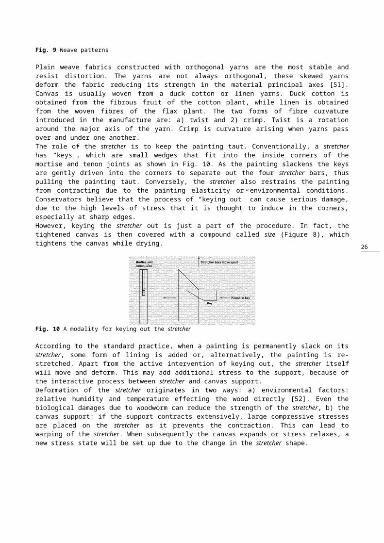
26

Fig. 19 Deformation map with tensioners at work

It is clear the effect of the increased strain along the y axis comparing Fig. 19 with the theoretical map shown in Fig. 13b. To obtain an assessment of the ratio of the strains on the two axes, i.e., the parameter which characterizes the canvas, it is possible to compare the experimental profiles along the two axes with the theoretical ones of Figs. 21c and 21d.From this comparison (see Figs. 20a and 20b), it is obtained that the experimental profiles has an R value between R = 1.78 and R = 7.11.

(a) (b)Fig.20 Experimental profiles of deformation along the median axes, compared with the theoretical ones corresponding to two different values of the R parameter

This result can be enhanced acting on the vertical tensioners. An example is shown in Fig. 21a. The reverse result is expected acting on the horizontal tensioners (Fig. 21b). The deformation map shows the pattern variations moving from one quadrant to another one, due to the fact that the strain along the x axis varies as a function of y.

(a) (b)

27

Fig. 21 Deformation maps corresponding to a strain along (a) the minor side, and (b) the major side

The stress imposed at the center of the canvas was of the order of tens of microns, corresponding to tens of fringes.After the mechanical test of the canvas performed by HI method, a NDT integrated approach useful to discover fabricated and natural defects has been realized on the final sample that reflects the typical constitution schematized in Fig. 8. In particular, the painting on canvas was firstly inspected by square pulse thermography (SPT) and after analyzed by pulsed phase thermography (PPT) and principal component thermography (PCT) techniques [44-48]. Both techniques were applied in a first stage on the paint layer (i.e., the sequence of thermograms was taken before the sample was varnished – Figs. 22 a,b), and in a second stage on the varnish layer (i.e., the sequence of thermograms was taken after the sample was varnished – Figs. 22 c-e). The latter is the top layer of the sample (Fig. 8), and on it, the DE-HI, the DSP by PIV, the UV imaging, and the NIRR techniques were also used to integrate the IRT data obtained [6-8, 55-57]. The remaining NDT techniques were applied only on the final sample. The main results are shown in Figs. 22a-r and the discussion is subsequently proposed.

(a) (b) (c) (d)

(e) (f) (g) (h)

(i) (l) (m) (n)

(o) (p) (q) (r)Fig. 22 (a) EOF3 – linked to the painting layer, (b) phasegram (f = 0.04 Hz) – linked to the painting layer, (c) EOF3 – linked to the varnish layer, (d) phasegram (f = 0.04 Hz) – linked to the varnish layer, (e) EOF6 – linked to the varnish layer , (f) rear side – clipping of the rectangular area (dotted rectangle) in Fig. 22e, (g) NIRT at 680 nm using one halogen lamp (OSRAM SICCATHERM – 250 W IR), (h) overlapping between the visible image of the zone inherent the defect A and the result of the LSI [22-25], (i) NIRR – clipping of the zone inherent the defect A, working with a LEDs lamp at 940 nm, (l) UV imaging in transmission mode – clipping of the zone inherent the defect A, working with a filter and an illuminator at 360 nm, (m) NIRR – clipping of the zone inherent the defect B, working with a LEDs lamp at 940 nm, (n) overlapping between the visible image of the zone inherent the defect B and the result of the LSI, (o) DE-HI of the zone inherent the defect B, the stretcher effect of the frame-canvas system, and the influence of a repair on the

A

BD

CE

Rear side

α

β

γ

E

28

fringes’ system, (p) DE-HI of the zone inherent the defects A and D; MatPIV manual [27]: (q) DSP result of the defect D (dry sponge), (r) DSP result of the defect D (dampened sponge: 15 ml of water)

The main difference between the IRT results in Figs. 22a-d is the detection of the defect C by PPT technique. For the sake of simplicity, the others EOFs images are not reported; however, defect C is not visible neither working on the paint layer, nor working on the varnish layer. The same thermocamera (FLIR S65 HS, 7.5 – 13 μm) and two lamps (Philips R125 IR S) were used during the IRT inspections. In order to preserve the artwork, two slight thermal stresses were applied: 5 s (Figs. 22a,b) and 10 s (Figs. 22c-e) of heating [58-61]. The repairs were detected by PCT technique (Fig. 22e) with a good contrast and minimizing the influence of the emissivity variation. Some repairs, which are visible to the naked eye on the rear side of the canvas, are surrounded by dotted ovals in Fig. 22f. Others repairs are visible using NIRT (defect E in Fig. 22g) and slightly in Fig. 22b, i.e., when the varnish layer is not applied yet. It is interesting to note how: 1) the LSI approach is useful to reveal the Mylar® inserts relative to the defects A (Fig. 22h) and B (Fig. 22n). The speckle contrast image enhances the target appearance and smoothes out the inhomogeneous background, 2) the NIRR (Fig. 22i) and the UV imaging transmittography (Fig. 22l) techniques, if applied together on the same zone, are capable to detect a subsurface defect (defect A) that simulates a detachment, showing an “encrusted area” and a reverse color of the peaks, 3) the same considerations about the integration between the LSI (Fig. 22n) and the NIRR (Fig. 22m) techniques are valid for the detection of the defect B, although realized of only one layer of Mylar®, 4) the DE-HI technique reveals, in addition to the fabricated defects (Figs. 22o,p), the stretcher effect which works near to the frame-canvas border (dotted irregular line), and not the internal border of the frame (dotted regular line) already retrieved by PPT technique (Fig. 22b), as well as a large repair of the canvas (solid irregular line) [22-25]. These lines form in Fig. 22o three different zones identified by three different configurations of the fringes (α, β, γ). The possibility of identifying into a unique image the stretcher effect and a subsurface repair demonstrates that the sensitivity of holography is very high thanks to the high resolution of holographic plates (3000 lines/mm – Table 1), and the table used during the experiment has a high degree of optical and mechanical stability. In fact, rigid body translation, causes the fringes to be localized away from the object surface. If this happens, it is more difficult to relate the fringe position to the object coordinates as in the case here treated.The behavior of the painting under the UV inspection (Fig. 22l) can be due to its shorter wavelength. The choice of working in transmission mode can be explained considering that UV radiation is much more scattered by surface layer, so it is not penetrating more than the varnish layer.The DE interferograms were acquired in thermal drift using a texp = 1s and a ti = 6 min. In this case, a blow dryer as thermal stress method was used. As said in the section 2.1, the attention that the holographic operator give to the environmental parameters (temperature and relative humidity) during the phase recording is maximum. In the present case, the relative humidity was maintained at 43% in each experiment, while the temperature surface of the painting was increased to 3 °C above the ambient temperature. Indeed, the necessity to record, develop and then reconstruct the hologram make it an involved and inflexible process. In the worst case, temperature and relative humidity affect the holographic gelatin emulsion causing swelling and shrinkage, 5) the cross-correlation approach seems to be very promising in order to detect the influence of the humidity on the varnish layer through a sponge soaked of 15 ml of water. In particular, Fig. 22q shows the DSP result obtained with the dry sponge, while Fig. 22r illustrates the effect of the water, comparing two images separated by a time of 1 hour and half, 6) since an imaging system is able to differentiate between the background reflectance of the underdrawing and the background reflectance of the ground when the paint layer thickness is less than the hiding thickness, we can assume that the paint layer thickness of the real and the reproduced artwork it is not the same; in fact, the author’s pentimento and his signature are not identifiable by NIRR, seeing Figs. 22i-m [11], [27]. A future experiment will explore the potentiality of the short-wave infrared (SWIR) reflectography for the present case, because if the paint is not too thick, the optimum wavelength to see through the paint while maintaining the ability to detect the graphite lines against a white background has been shown around 2 μm [62]. Finally, in Table2 are reported the fabricated and natural defects vs. the NDT techniques applied on the La Crocifissione di Sansepolcro painting. This Table can help to understand the importance of an integrated NDT approach in the field of cultural heritage because, at the moment, it doesn’t exist a unique method able to discover and/or identify and/or characterize the totality of sub-superficial discontinuities linked to the structure or the history (for example, repairs) of the artwork under analysis.

Defect LSI DSP HI UV NIRR NIRT PPT PCTA * ° * ↄ ↄ ^ * *B * ° * ° * ^ * *

29

C ° ° ° ° ° ^ * ^D ° ↄ * ° ° ^ * *E ° ° ^ ° ° * * ^

repairs ^ ^ * ^ ^ ^ ^ *stretcher effect ° ↄ ↄ ° ° ^ ^ ^

Tab. 2 NDT techniques vs. fabricated and natural defects. Legend: (*) analyzed and identified, (°) not analyzed, (^) analyzed but not identified, (ↄ) analyzed, identified and characterized, (ↄ) analyzed, identified and characterized by an integrated approach

5. CONCLUSIONSThe purpose of this work is to study the detection of defects already present or artificially induced in a painting on canvas by mechanical stress or other factors. A first result obtained is that the structure of the canvas does not determine the trend of the interference pattern, i.e. the intensity distribution of the fringes is the same that would occur in a continuous means. Another factor which is worthy to point out is that the trend of the fringes is generally regular, i.e. also in the case where the shape of the fringes is not directly comparable with the theoretical models (for example, where the shape of the fringes varies from a quadrant to another one of the canvas), no local irregularity is highlighted into a small scale respect to the linear dimensions of the canvas. In the case of the painting on canvas, it is possible to think that, when local irregularities are detected, they can be attributed to defects of homogeneity in the surface layers. This assumption is confirmed comparing the double-exposures made before and after that the canvas was painted (Figs. 21a,b and Figs. 22o,p). A third result to be underlined is that, for a number of cases in which the canvas is uniformly stretched on the frame or it is straining in a different way along the parallel directions to the edges, but with strain levels that remain constant along each edge, a simple mathematical model which treats the canvas-frame structure as a membrane fixed along the rectangular border is able to explain in a satisfactory manner the behavior of the canvas itself [63]. This method provides an interpretation’s base for the analysis of more complex patterns, and it permits to exalt the contribution of the optical and infrared NDT techniques when applied to the defects detection and their characterization, even if linked to dynamic, i.e. humidity (Figs. 22q,r), or technical variables, i.e. number of layers (Figs. 22a-d), thickness/depth of the defect under inspection (Figs. 22e-n), and the stretcher effect (Figs. 22o,r).Finally, two interesting perspectives of the work, would be: a) to perform an “in situ” investigation of historic paintings using, at least partially, the proposed approach, and b) to work using a non-uniform strain in correspondence to the edges of the canvas model, because it is also possible to find situations where the canvas nailed to the stretcher exhibits so called “canvas cuspings”.

REFERENCES

[1] Hackney S, Hedley G (1993) In: Villers C (ed) Measured opinion, UKIC, London[2] Hedley G (1993) In: Villers C (ed) Measured opinion, UKIC, London[3] Berger BA, Russell WH (1988) An evaluation of canvas paintings using stress measurements. Stud Conserv 33:

187-204 [4] Clulow EE, Taylor HM (1963) An experimental and theoretical investigation of biaxial stress-strain relations in

a plain-weave cloth. J Text I 54(8):323-347. [5] Paoletti D, Schirripa G, D’Altorio A (1985) Sandwich hologram: a practical tool for stress analysis in paintings

on canvas. Proc. SPIE 0599. Doi: 10.1117/12.952360[6] van Asperen de Boer JRJ (1966) Infrared reflectograms of panel paintings. Stud Conserv 11:45-46 [7] Lizun D (2011) Fine art conservation – Ultraviolet radiation. http://fineartconservation.ie/damian-lizun-fine-art-

conservation-4-4-43.html, accessed on 01 October 2013[8] Ambrosini D, Paoletti D, Galli, G (2008) In: Castillejo M (ed) Lasers in the conservation of artworks, Taylor &

Francis Group, London[9] Gülker G, Hinsch KD, Kraft A (2000) In: Jacquot P, Fournier J-M (eds) Interferometry in speckle light. Theory

and applications, Springer, Germany

30

[10] Ibarra-Castanedo C, Sfarra S, Ambrosini D, Paoletti D, Bendada A, Maldague X (2010) Diagnostics of panel paintings using holographic interferometry and pulsed thermography. QIRT J 7(1):85-114

[11] van Asperen de Boer JRJ (1970) Infrared reflectography: a contribution to the examination of earlier European paintings. Central research laboratory for objects of art and science, Amsterdam

[12] Vest CM (1979) Holographic Interferometry. Wiley, New York[13] Jones R, Wykes C (1983) Holographic and speckle interferometry: a discussion of the theory, practice and

application of the techniques. Cambridge University Press, New York[14] Rowlands RE, Daniel IM (1972) Application of holography to anisotropic composite plates. Exp Mech

12(2):75-82[15] Sampson RC (1970) Holographic-interferometry applications in experimental mechanics. Exp Mech 10(8):313-

320[16] Friedberg PD (2004) Applications of holography: interferometry for mechanical stress and vibration

measurement. http://www-inst.eecs.berkeley.edu/~ee119/sp09/EE290F_Fall2004_PD_Friedberg.pdf, accessed on 01 October 2013

[17] Paoletti D, Schirripa Spagnolo G, D’Altorio, A (1989) The state of art of holographic non destructive testing in work of art diagnostics. Revue Phys Appl 24:389-399

[18] Sirohi RS (1993) Speckle metrology. Marcel Dekker, New York[19] Sjödahl M (1988) Some recent advances in electronic speckle photography. Opt Laser Eng 29:125-144[20] Sjödahl M (1997) Accuracy in electronic speckle photography. Appl Opt 36:2875-2885[21] Li J, Yao G, Wang LHV (2002) Degree of polarization in laser speckles from turbid media: implications in

tissue optics. J Biomed Opt 7:307-12  [22] Nothdurft R, Yao G (2005) Imaging obscured subsurface inhomogeneity using laser speckle. Opt Express

13(25):10034-10039[23] Cheng H, Luo Q, Zeng S, Chen S, Cen J, Gong H (2003) Modified laser speckle imaging method with

improved spatial resolution. J Biomed Opt 8(3):559-564[24] Draijer M, Hondebrink E, van Leeuwen T, Steenbergen W (2009) Review of laser speckle contrast techniques

for visualizing tissue perfusion. Lasers Med Sci 24(4):639-651[25] Kirkpatrick SJ, Duncan DD, Wang RK, Hinds MT (2007) Quantitative temporal speckle contrast imaging for

tissue mechanics. J Opt Soc Am A 24:3728-34[26] Nandigana KM (2000) In: Yoshizawa T (ed) Handbook of optical metrology. Principles and applications, CRC

Press, U.S.A.[27] Astarita T (2006) Analysis of interpolation schemes for image deformation methods in PIV. Exp Fluids 38:233-

243[28] Bastiaans RJM (2000) Cross-correlation PIV; theory, implementation and accuracy.

http://alexandria.tue.nl/repository/books/531139.pdf, accessed on 01 October 2013[29] Pelagotti A, Pezzati L, Piva A, Del Mastio A (2006) Multispectral UV fluorescence analysis of painted

surfaces. http://www.eurasip.org/Proceedings/Eusipco/Eusipco2006/papers/1568987270.pdf, accessed on 01 October 2013

[30] Richards A (2006) Digital reflected-ultraviolet imaging. http://www.uvcorder.com/pdf/ADI0406%20Component%2018-20.pdf, accessed on 01 October 2013

[31] Webber SL (2008) Technical imaging of paintings. http://www.williamstownart.org/techbulletins/images/WACC%20Imaging%20of%20Paintings.pdf, accessed on 01 October 2013

[32] Walmsley E, Fletcher C, Delaney J (1992) Evaluation of system performance of near-infrared imaging devices. Stud Conserv 37:120-131

[33] Kossolapev AJ (1993) An improved vidicon TV camera for IR-Reflectography. ICOM Committee for Conservation, 10th triennial meeting. Science Publishers Ltd, Washington

[34] Real W (1985) Exploring new applications for infrared reflectography. B Cleveland Mus Art 72:390–412[35] Wecksung G, Evans R, Walker J, Ainsworth M, Brealey, J, Carriveau, GW (1987) Assembly of infra-red

reflectograms by digital processing using a portable data collecting system. ICOM Committee for Conservation, 8th triennial meeting. The Getty Conservation Institute, Sydney

[36] Delaney JK (1993) Examination of the visibility of underdrawing lines as a function of wavelength. ICOM Committee for Conservation, 10th triennial meeting. Science Publishers Ltd, Washington

31

[37] Bertani D, Buzzegoli E, Cecchi S, Cetica M, Kunzelman D, Piccioni GP, et al (1990) A scanning device for infrared reflectography. Stud Conserv 35:113–6

[38] Coddington J (1991) The use of infra-red vidicon and image digitizing software in examining 20 th century works of art. AIC paintings specialty group postprints – 19th annual meeting of the AIC. American Institute for conservation of historical and artistic works, Albuquerque

[39] Astheimer RW (1983) Handbook of infrared radiation measurement. Barnes Engineering Company, Stamford[40] Weiner C (1998) Improved acquisition of underdrawings in oil-paintings using IR-Reflectography. Final report

SIMG-503. Rochester Institute of Technology, Rochester[41] Sfarra S, Ibarra-Castanedo C, Paoletti D, Maldague X (2013) Infrared vision inspection of cultural heritage

objects from the city of L’Aquila, Italy and its surroundings. Mater Eval 5:561-570[42] Lerma JL, Cabrelles M, Portalés C (2011) Multitemporal thermal analysis to detect moisture on a building

façade. Constr Build Mater 25(5):2190-7[43] Arndt RW (2010) Square pulse thermography in frequency domain as adaptation of pulsed phase thermography

for qualitative and quantitative applications in cultural heritage and civil engineering. Infr Phys Technol 53:246-53

[44] Maldague X, Marinetti S (1996) Pulse phase infrared thermography. J Appl Phys 79:2694-8  [45] Larsen CA (2011) Document flash thermography. http://digitalcommons.usu.edu/cgi/viewcontent.cgi?

article=2020&context=etd, accessed on 01 October 2013[46] Parvataneni R (2009) Principal component thermography for steady thermal perturbation scenarios.

http://etd.lib.clemson.edu/documents/1263397875/Parvataneni_clemson_0050M_10470.pdf, accessed on 01 October 2013

[47] Rajic N (2002) Principal component thermography for flaw contrast enhancement and flaw depth characterisation in composite structures. Compos Struct 58:521-8

[48] Rajic N (2002) Principal component thermography. http://www.dsto.defence.gov.au/publications/2452/DSTO-TR-1298.pdf, accessed on 01 October 2013

[49] Émile-Mâle G (1976) The restorer’s handbook of easel paintings. Van Nostrand Reinhold, New York[50] Hedley G, et al. (1994) In: Villers C (ed) Measured opinion, UKIC, London[51] Zweben C, Norman JC (1976) Kevlar 49/Thornel 300 hybrid fabric composites for aerospace applications.

SAMPE Quarterly 1-10[52] Fryxell RE (1981) Further observations on moisture breathing of wood. Catgut Acous Soc News 35:7-11[53] Paolucci A (2004) Luca Signorelli – Pittori del Rinascimento. Scala, Firenze[54] Young CRT (1996) Measurement of biaxial tensile properties of paintings on canvas. Exhibition Rd., London[55] Kreis T (2005) Handbook of holographic interferometry. Wiley-VCH, Federal Republic of Germany[56] Raffel M, Willert CE, Wereley ST, Kompenhans J (2007) Particle image velocimetry – A practical guide.

Springer-Verlag, Berlin[57] Gilblom DL, Yoo SK (2004) Infrared and ultraviolet imaging with a CMOS sensor having layered photodiodes.

Proc SPIE 5301. Doi: 10.1117/12.528427[58] Ambrosini D, Daffara C, Di Biase R, Paoletti D, Pezzati L, Bellucci R, Bettini F (2010) Integrated

reflectography and thermography for wooden paintings diagnostics. J Cult Herit 11(2):196-204[59] Bodnar JL, Candoré JC, Nicolas JL, Szatanik G, Detalle V, Vallet JM (2012) Stimulated infrared thermography

applied to help restoring mural paintings. NDT&E Int 49:40-46[60] Avdelidis NP, Moropoulou A (2004) Applications of infrared thermography for the investigation of historic

structures. J Cult Herit 5(1):119-127[61] Gavrilov D, Maeva E, Grube O, Vodyanoy I, Maev R (2013) Experimental comparative study of the

applicability of infrared techniques for non-destructive evaluation of paintings. J Am Inst Conserv 52(1):48-60[62] Vollmer M, Mӧllmann KP (2010) Infrared thermal imaging – fundamentals, research and applications. Wiley-

VCH, Federal Republic of Germany[63] Amadesi S, Gori F, Grella R, Pasquini P, Guattari G (1973) In: Compositori (ed) Problemi di conservazione II,

Bologna, Italy