Narrow-Band Processing and Fusion Approach for Explosive Hazard Detection in FLGPR

Timothy C. Havens*a, James M. Kellera, K.C. Hoa,

Tuan T. Tonb, David C. Wongb, and Mehrdad Soumekhc aDept. of Electrical and Computer Engineering, University of Missouri, Columbia, MO, USA 65211;

bU.S. Army REDCOM CERDEC NVESD, Fort Belvoir, Virginia, USA 22060; cDept. Of Electrical Engineering, University of New York at Buffalo, Amherst, NY, USA 14260

ABSTRACT

This paper proposes an effective anomaly detection algorithm for a forward-looking ground-penetrating radar (FLGPR). One challenge for threat detection using FLGPR is its high dynamic range in response to different kinds of targets and clutter objects. The application of a fixed threshold for detection in a full-band radar image often yields a large number of false alarms. We propose a method that uses both narrow-band and full-band radar processing, coupled with a classifier that uses complex-valued Gabor filter responses as the features. We then fuse the narrow-band and full-band images into a composite confidence map and detect local maxima in this map to produce candidate alarm locations. Full-band radar images provide a high degree of image resolution, while narrow-band images provide a means to detect targets which have a unique narrow-band signature. Experimental results for our improved detection techniques are demonstrated on data sets collected at a US Army test site.

Keywords: forward-looking explosive hazards detection, ground-penetrating radar, narrow-band processing, false alarm rejection, fusion, Gabor filters

1. INTRODUCTION Remediation of the threat of explosive hazards is an extremely important goal, as these hazards are responsible for uncountable deaths and injuries to both civilians and soldiers throughout the world. Systems that detect explosive hazards have included ground-penetrating-radar (GPR), infrared (IR) cameras, and acoustic technologies.1-3 Both handheld and vehicle-mounted GPR-based systems have been examined in recent research and much progress has been made in increasing detection capabilities.4,5 Forward-looking synthetic aperture GPR (FLGPR) is an especially attractive technology because of its ability to detect hazards before they are encountered; standoff distance can range from a few to tens of meters. FLGPR has been applied to the detection of side-attack mines6, and mines in general.7,8 A drawback to these systems is that FLGPR is not only sensitive to objects of interest, but also to other objects, both above and below the ground. This results in an excessive number of FAs.

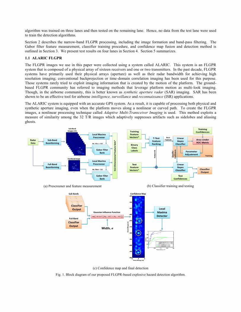
Figure 1 illustrates our proposed FLGPR-based explosive hazard detection algorithm. View (a) illustrates the prescreener and feature measurement approach. A prescreener detects local maxima in the full-band and narrow-band images and then a filter band of Gabor filters is used to measure the texture content of images at each prescreener alarm. These features are passed to a classifier, shown in view (b), which uses a statistical feature selection method to pick the best feature from which to classify true positive from false alarms. A classifier is then trained on this best feature to produce the best Area-Under-ROC (AUR). Finally, the classifier results from the full-band and each narrow-band image are fused into a grid-based confidence map, as shown in view (c). The local maxima are detected in this confidence map to determine the candidate alarm locations. We will show in Section 4 that the proposed approach can reduce the false alarm rate in test data by greater than 50%, while maintaining a detection rate comparable to using just a threshold-based prescreener.

The data used in this paper are composed of four runs of the FLGPR system at a US Army test facility. We will call these runs, Lanes 1, 2, 3, and 4. These data consist of two runs down one test road and two runs down another test road, each with slight changes to the hardware configurations—although, we currently do not consider these slight changes as having an impact on the relative performance. The results shown are test results, which means that the detection

algorithm was trained on three lanes and then tested on the remaining lane. Hence, no data from the test lane were used to train the detection algorithms.

Section 2 describes the narrow-band FLGPR processing, including the image formation and band-pass filtering. The Gabor filter feature measurement, classifier training procedure, and confidence map fusion and detection method is outlined in Section 3. We present test results on four lanes in Section 4. Section 5 summarizes.

1.1 ALARIC FLGPR

The FLGPR images we use in this paper were collected using a system called ALARIC. This system is an FLGPR system that is composed of a physical array of sixteen receivers and one or two transmitters. In the past decade, FLGPR systems have primarily used their physical arrays (aperture) as well as their radar bandwidth for achieving high resolution imaging; conventional backprojection or time-domain correlation imaging has been used for this purpose. Those systems rarely tried to exploit imaging information that is created by the motion of the platform. The ground-based FLGPR community has referred to imaging methods that leverage platform motion as multi-look imaging. Though, in the airborne community, this is better known as synthetic aperture radar (SAR) imaging. SAR has been shown to be an effective tool for airborne intelligence, surveillance and reconnaissance (ISR) applications.

The ALARIC system is equipped with an accurate GPS system. As a result, it is capable of processing both physical and synthetic aperture imaging, even when the platform moves along a nonlinear or curved path. To create the FLGPR images, a nonlinear processing technique called Adaptive Multi-Transceiver Imaging is used. This method exploits a measure of similarity among the 32 T/R images which adaptively suppresses artifacts such as sidelobes and aliasing ghosts.

(a) Prescreener and feature measurement

(b) Classifier training and testing

(c) Confidence map and final detection

Fig. 1. Block diagram of our proposed FLGPR-based explosive hazard detection algorithm.

Table 1 contains the parameters of the ALARIC FLGPR that were used to create the images used in this paper.

The FLGPR images are created for an area -11 to +11 meters in the cross-range direction—although only the -5 to +5 meter cross-range sub-region is used in our detection algorithms—where negative numbers indicate to the left of the vehicle. Coherent integration of the radar scans is done in an area 5-10 meters in front of the vehicle. The pixel-resolution of the FLGPR image is 5 cm in the down-range and 3 cm in the cross-range directions. The center frequency is 800 MHz and the bandwidth is 1.4 GHz. The detection region we use is 10 meters wide, centered in the cross-range direction. References 9-13 describe our previous efforts in detecting explosive hazards using FLGPR; the prescreener algorithm we use here is also used in this previous work.

1.2 Prescreener

Consider an FLGPR image, �(�, �), where � is the cross-range coordinate and � is the down-range coordinate. This image is input to a local-maxima finding algorithm to determine candidate alarm locations. Our method first computes a maximum order-filtered image with a 3 m x 1 m kernel. We denote this order-filtered image as �(�, �). Essentially, each pixel in the FLGPR image is replaced by the maximum pixel value within a 3 m cross-range and 1 m down-range rectangle, centered on the pixel. Figure 2 shows an example of an FLGPR image and its associated order-filtered image. As this figure shows, the order-filter reduces the effect that noise-induced artifacts have on finding “hot spots” in the image. Alarms are identified by the operation

� = ��(,�){�(�, �) ≥ min{�(�, �), −90}}, where A is the set of local-maxima locations. The minimum operator prescreens alarm locations that have a very low

Table 1. ALARIC FLGPR image-forming parameters Parameter Value

Coherent integration range 5 – 10 meters down-range Full-band bandwidth

Narrow-band bandwidth 100 MHz – 1.5 GHz

100 MHz (14 narrow-bands from 100MHz to 1.5 GHz) Down-range image resolution 5 cm Cross-range image resolution 3 cm Cross-range detection limits -5 to +5 meters

Fig. 2. Local maxima prescreener example—alarm locations shown as white circles, target locations shown as red circles.

FLGPR image value (confidence). We chose a value of -90 dB for this threshold as this only eliminates alarms with the lowest of confidences. This prescreening threshold merely minimizes the computational cost of the subsequent algorithms by reducing the number of alarms to a manageable number. We also annotate the alarm locations A with the value of the FLGPR image pixel at each location, which we denote as �(�). This pixel value is, in effect, the confidence of the alarm—the higher the value, the higher the confidence. Figure 2 illustrates the prescreener process, including the alarm locations for the example images shown.

We use this prescreener on both the full-band FLGPR image as well as the 14 narrow-band images.

1.3 Area Under ROC (AUR)

The AUR metric is used in the training of the classifiers as well as to show the relative efficacy of the different detection methods that we employ. This metric is simply the normalized area under the resulting receiver-operating characteristic (ROC) curve for a given detector. Figure 4 illustrates how we calculate this metric for an example ROC curve. We chose a maximum false alarms per meter-squared rate of 0.2 at which to limit the AUR calculation and calculate the AUR by

� � = 10.2� ��(�)��

�.�

�,

where ��(�) is the probability of detection at a given false alarm rate of �. Notice that the minimum AUR is 0, which indicates that ��(�) = 0 for all �, and the maximum AUR is 1, which indicates perfect probability of detection with zero false alarms.

1.4 Miss-distance halo size

In this paper, we present results for two different miss-distances: 2 meter and 1 meter radius halos. While we believe that 2 m halos are excessive in size (imagine trying to dig something up in a 4 meter wide circle), the role of FLGPR in the battlefield has not yet been established and, thus, we wish to be comprehensive about the results we present. There are many mechanisms of error in FLGPR that do not exist in downward-looking sensors, such as refraction at the air-ground boundary and other soil boundary layers, longer range imaging (which accentuates geo-location-based errors), and low-grazing angle specular ground-bounce. As of yet, a comprehensive understanding of how these sources of error manifest into miss-distances does not exist. Furthermore, we believe that FLGPR can operate as an early-warning sensor, cueing operators to the presence of targets ahead. The operators can then slow down and use a downward-looking system to more accurately locate the hazard. This allows operators to overall travel at higher speeds, covering more terrain in less time.

Next we describe the narrow-band processing and image formation.

2. NARROW-BAND FLGPR PROCESSING The spatial resolution in FLGPR images is directly related to the bandwidth of the range spectrum used to produce those images. Hence, we expect that the full-band images will have the best overall image quality. However, it has been

Fig. 3. Area Under ROC (AUR) metric calculation.

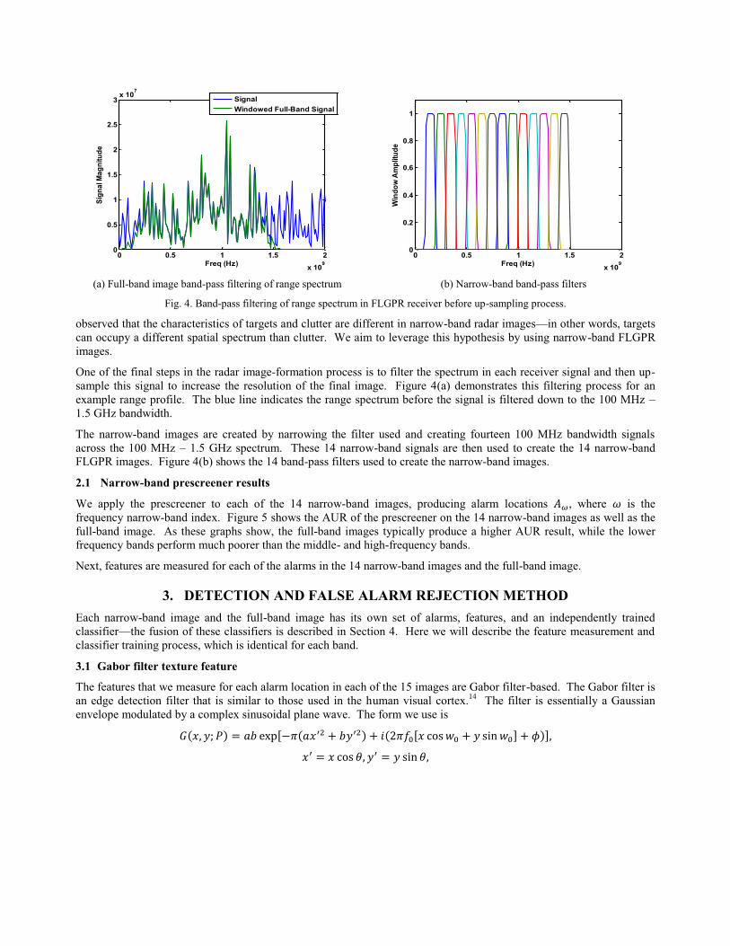
observed that the characteristics of targets and clutter are different in narrow-band radar images—in other words, targets can occupy a different spatial spectrum than clutter. We aim to leverage this hypothesis by using narrow-band FLGPR images.

One of the final steps in the radar image-formation process is to filter the spectrum in each receiver signal and then up-sample this signal to increase the resolution of the final image. Figure 4(a) demonstrates this filtering process for an example range profile. The blue line indicates the range spectrum before the signal is filtered down to the 100 MHz – 1.5 GHz bandwidth.

The narrow-band images are created by narrowing the filter used and creating fourteen 100 MHz bandwidth signals across the 100 MHz – 1.5 GHz spectrum. These 14 narrow-band signals are then used to create the 14 narrow-band FLGPR images. Figure 4(b) shows the 14 band-pass filters used to create the narrow-band images.

2.1 Narrow-band prescreener results

We apply the prescreener to each of the 14 narrow-band images, producing alarm locations ��, where � is the frequency narrow-band index. Figure 5 shows the AUR of the prescreener on the 14 narrow-band images as well as the full-band image. As these graphs show, the full-band images typically produce a higher AUR result, while the lower frequency bands perform much poorer than the middle- and high-frequency bands.

Next, features are measured for each of the alarms in the 14 narrow-band images and the full-band image.

3. DETECTION AND FALSE ALARM REJECTION METHOD Each narrow-band image and the full-band image has its own set of alarms, features, and an independently trained classifier—the fusion of these classifiers is described in Section 4. Here we will describe the feature measurement and classifier training process, which is identical for each band.

3.1 Gabor filter texture feature

The features that we measure for each alarm location in each of the 15 images are Gabor filter-based. The Gabor filter is an edge detection filter that is similar to those used in the human visual cortex.14 The filter is essentially a Gaussian envelope modulated by a complex sinusoidal plane wave. The form we use is

�(�, �; �) = �� exp[−�(���� + ����) + �(2���[� cos � + � sin �] + !)], �� = � cos ", �� = � sin ",

(a) Full-band image band-pass filtering of range spectrum

(b) Narrow-band band-pass filters

Fig. 4. Band-pass filtering of range spectrum in FLGPR receiver before up-sampling process.

0 0.5 1 1.5 2

x 109

0

0.5

1

1.5

2

2.5

3x 107

Freq (Hz)

Sign

al M

agni

tude

SignalWindowed Full-Band Signal

0 0.5 1 1.5 2

x 109

0

0.2

0.4

0.6

0.8

1

Freq (Hz)

Win

dow

Ampl

itude

(a) Lane 1 – 1 meter halo (a) Lane 2 – 1 meter halo

(a) Lane 3 – 1 meter halo (a) Lane 4 – 1 meter halo

(a) Lane 1 – 2 meter halo (a) Lane 2 – 2 meter halo

(a) Lane 3 – 2 meter halo (a) Lane 4 – 2 meter halo

Fig. 5. Prescreener Results. Full-band results shown as band #15.

where � = {�, �, ", ��, �, !} is the set of filter parameters: a and b are the widths of the Gaussian envelope, " is the rotation angle of the envelope, �� is the frequency of the sinusoid, � is the rotation of the sinusoid, and ! is the phase. Figure 6 shows two examples of Gabor filters.

We convolve a filter bank composed of 512 different Gabor filters with the FLGPR images at each alarm location (in each of the 15 images). The parameters of the 512 filters are all possible combinations of those shown in Table 2. Hence, the features for each band are

#(��; �) = $ $ �(�, �; �) ∗ ��(�&' − �, �&' − �)*�

-/3*�

*�

4/3*�, ∀��, ∀�,

where �� is the �-band image. Notice that F is a 512-dimensional vector for each alarm in ��.

Now we have a 512-dimensional feature vector that describes each alarm in each of the 15 images. Next we determine which feature will be the best for separating true positives from false alarms.

3.2 Feature selection

We concatenate the features from three training lanes and use a two-sample t-test with pooled variance estimate to rank the features. The two-sample t-test simply provides a measure of how well-separated the means of two sample-based distributions are with respect to their variance. Assume that #3 is the set of features for the false alarms and #6 are the features for the true positives. First, the pooled variance estimate is calculated by

Table 2. Gabor filter bank parameters.

Parameter Value

1/a, 1/b 30, 60 pixels

" 0, 45, 90, 135 degrees

1/�� 10, 20 pixels per cycle

� 0, 90, 180, 270 degrees

! 0, 8: ,8� ,<8: radians

Total of 512 filters

(a) � = ><� , � =

><� , " = 0, �� =

>�� , � = 90,! =

<8:

(b) � = >?� , � =

><� , " = 45, �� =

>>� , � = 180,! =

<8:

Fig. 6. Examples of complex-valued Gabor filters. Real part of filter shown.

Pixels

Pixe

ls

20 40 60 80 100

10

20

30

40

50

60

70

80

90

10020 40 60 80 100

10

20

30

40

50

60

70

80

90

100

Pixels

Pix

els

where C3 is the number of false alarms, C6 is the number of true positives, D3� is the sample-based variance of the false alarms, and D6� is the sample-based variance of the true positives. The t-test is computed as

where �3EEE and �6EEE are the sample-based means of the false alarms and true positives, respectively. The larger the value of t, the greater the separation of the means with respect to the pooled variance estimate.

We perform the t-test on each dimension of the feature vector F and keep the feature with the highest t-test value. We then use this best feature to train a classifier.

Other feature ranking methods were tried, including AUR, KL divergence, and Bhattacharyya distance; the two-sample t-test provided the best test results on the test data we had.

3.3 False alarm rejecting classifier

Assume that Fbest is the feature chosen by our feature selection method. We take this feature from the three training lanes and train a linear classifier to discriminate true positives from false alarms. First, we fit a normal distribution with a pooled variance estimate to the feature values from each class in the training data. We use a pooled variance estimate because the number of true positives in the data is very small compared to the false alarms; hence, an accurate variance estimate for the true positives is unattainable. Assume that �(+|#) is the resulting probability of a true positive given an input feature value and �(−|#) is the probability of a false alarm. Hence, the resulting classifier, for a given input feature F, is simply

FG�HH(#) = I+ �(+|#)�(+) ≥ �(−|#)�(−)− JGHJ ,

where �(+) and �(−) are the prior probabilities. We use the prior probabilities to tune the classifier to achieve the highest AUR of the output true positive class (which will, of course, include some false alarms).

(a) Test results for lane 1 – 1m halo

(b) Test results for lane 2 – 2m halo

(c) Test results for lane 3 – 1m halo

(d) Test results for lane 4 – 1m halo

Fig. 7. 1m halo ROC curves of Gabor filter classifier. Classifier results shown as green solid line, prescreener results shown as blue

0 0.05 0.1 0.15 0.20

0.2

0.4

0.6

0.8

1

False Alarms per m2

Prob

Det

Lane 1, 1m halo

0 0.05 0.1 0.15 0.20

0.2

0.4

0.6

0.8

1

False Alarms per m2

Prob

Det

Lane 2, 1m halo

0 0.05 0.1 0.15 0.20

0.2

0.4

0.6

0.8

1

False Alarms per m2

Prob

Det

Lane 3, 1m halo

0 0.05 0.1 0.15 0.20

0.2

0.4

0.6

0.8

1

False Alarms per m2

Prob

Det

Lane 4, 1m halo

We define the prior probabilities by a convex combination, 1 = K�(+) + (1 − K)�(−). Hence, K can be adjusted to change the behavior of the classifier. An K near to 1 will cause the classifier to bias heavily towards classifying input features as true positives, while an K near 0 will cause the classifier to bias towards false alarms. Although one could imagine that K could be tuned using a non-linear optimization method, such as a monte-carlo scheme or swarm optimization, we simply trained a classifier for each of K = {0.4, 0.45, 0.5, 0.55, 0.6, 0.65, 0.7}. The performance of the classifier for each value of K was measured by the resulting AUR of the alarrns classified as true positives. In other words, the training features were resubstituted into the classifier and the feature values (alarms) classified as true positive (+) were kept—the alarms classified as false alarms (-) were discarded. The ROC curve for the alarms that were kept was computed and the K that produced the highest AUR was chosen as the best.

Figures 6 and 7 shows the ROC curves for the output of the trained classifiers on four test lanes for the full-band images. These results are computed by training the classifier on three training lanes and then applying the classifier to the fourth test lane. In other words, lanes 1, 2, and 3 are used to train the classifier for lane 4; lanes 2, 3, and 4 are used to train the classifier for lane 1; etc. As Figs. 6 and 7 show, the classifier is able to reduce the number of false alarms and increase the AUR. It is interesting to note that the classifier on lane 2 for both the 1m and 2m halos has a reduced maximum probability of detection; however, the AUR in both cases is increased. Hence, although we use AUR here to train our classifiers, a different performance metric, such as false alarm rate at a specified probability of detection (say 90%), may be more appropriate, depending on the requirements of the specific application.

A separate classifier is trained for each narrow-band image and the full-band image, resulting in 15 classifiers. The output of these classifiers is a set of alarms: one set for each band. We now discuss how we take these 15 sets of alarms and fuse them together to determine a final composite set of alarm locations.

dotted line.

(a) Test results for lane 1 – 2m halo (b) Test results for lane 2 – 2m halo

(c) Test results for lane 3 – 2m halo (c) Test results for lane 4 – 2m halo

Fig. 8. 2m halo ROC curves of Gabor filter classifier. Classifier results shown as green solid line, prescreener results shown as blue dotted line.

0 0.05 0.1 0.15 0.20

0.2

0.4

0.6

0.8

1

False Alarms per m2

Prob

Det

Lane 1, 2m halo

0 0.05 0.1 0.15 0.20

0.2

0.4

0.6

0.8

1

False Alarms per m2

Prob

Det

Lane 2, 2m halo

0 0.05 0.1 0.15 0.20

0.2

0.4

0.6

0.8

1

False Alarms per m2

Prob

Det

Lane 3, 2m halo

0 0.05 0.1 0.15 0.20

0.2

0.4

0.6

0.8

1

False Alarms per m2

Prob

Det

Lane 4, 2m halo

3.4 Confidence map fusion and detection

In the final step of our algorithm, we combine the classification results from all 15 bands. The alarms in each of the 15 images do not occur in the same exact location; hence, we simply cannot stack the classifier outputs and produce a ROC curve. We produce an alarm confidence map, which is a grid-based map,

where each map pixel represents the confidence of an alarm at its corresponding location. This map is created by taking the classifier outputs—a set of alarm locations—from each of the 15 images and mapping the confidence of those alarms onto the confidence map by applying a Gaussian blurring function. Mathematically, this can be written as

N(C, J) = $$��(C, J)O

P/>

>*

�/>∗ Q RC − ST6U#(��, �VWXY)Z\^, J − ST6U#(��, �VWXY)Z\W_ ,

where ��(C, J) is the confidence value (pixel value in the radar image) of the alarm, ST6U#(��, �VWXY)Z\^ is the Northing location of the alarms classified as true positives in the � band image using the best Gabor feature, with parameters �VWXY, and ST6U#(��, �VWXY)Z\W is the Easting location of the alarms. The blurring function B has the following form

Q(C, J) = exp[(C� + J�) 2D�]⁄ , where D = 0.5 for our results.

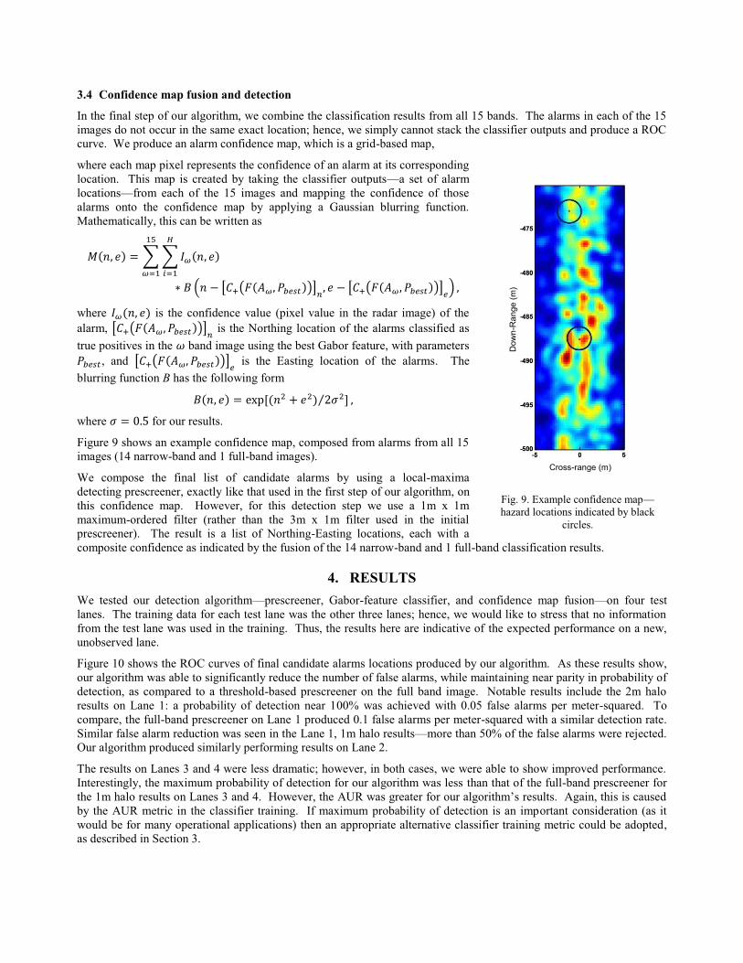
Figure 9 shows an example confidence map, composed from alarms from all 15 images (14 narrow-band and 1 full-band images).

We compose the final list of candidate alarms by using a local-maxima detecting prescreener, exactly like that used in the first step of our algorithm, on this confidence map. However, for this detection step we use a 1m x 1m maximum-ordered filter (rather than the 3m x 1m filter used in the initial prescreener). The result is a list of Northing-Easting locations, each with a composite confidence as indicated by the fusion of the 14 narrow-band and 1 full-band classification results.

4. RESULTS We tested our detection algorithm—prescreener, Gabor-feature classifier, and confidence map fusion—on four test lanes. The training data for each test lane was the other three lanes; hence, we would like to stress that no information from the test lane was used in the training. Thus, the results here are indicative of the expected performance on a new, unobserved lane.

Figure 10 shows the ROC curves of final candidate alarms locations produced by our algorithm. As these results show, our algorithm was able to significantly reduce the number of false alarms, while maintaining near parity in probability of detection, as compared to a threshold-based prescreener on the full band image. Notable results include the 2m halo results on Lane 1: a probability of detection near 100% was achieved with 0.05 false alarms per meter-squared. To compare, the full-band prescreener on Lane 1 produced 0.1 false alarms per meter-squared with a similar detection rate. Similar false alarm reduction was seen in the Lane 1, 1m halo results—more than 50% of the false alarms were rejected. Our algorithm produced similarly performing results on Lane 2.

The results on Lanes 3 and 4 were less dramatic; however, in both cases, we were able to show improved performance. Interestingly, the maximum probability of detection for our algorithm was less than that of the full-band prescreener for the 1m halo results on Lanes 3 and 4. However, the AUR was greater for our algorithm’s results. Again, this is caused by the AUR metric in the classifier training. If maximum probability of detection is an important consideration (as it would be for many operational applications) then an appropriate alternative classifier training metric could be adopted, as described in Section 3.

Fig. 9. Example confidence map—hazard locations indicated by black

circles.

Cross-range (m)

Dow

n-R

ange

(m)

4.1 Missed detections in 1m halo results

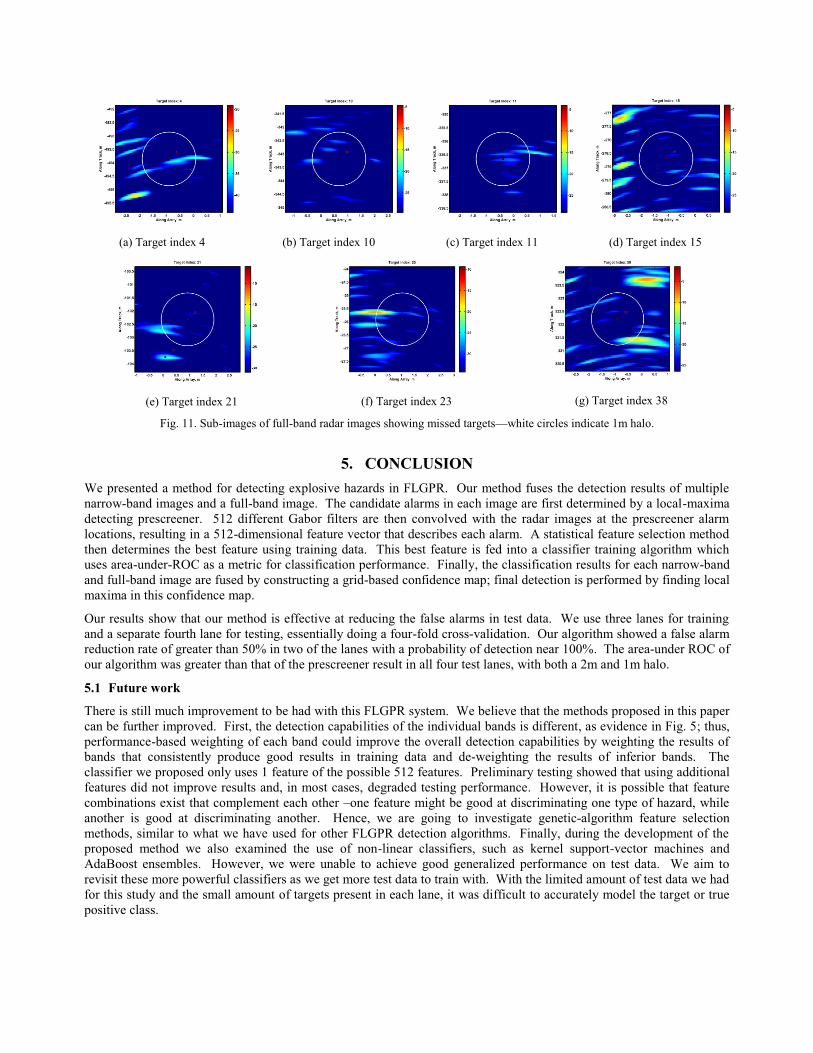
The results in Fig. 10 show that there were a significant number of hazards that were not detected with a 1m halo. We examined the full-band images of these targets to see why these hazards were not detected. Figure 11 shows 2m x 2m sub-images of the hazards that were missed in Lane 3 (we show Lane 3 because there were only 7 missed targets, which is a more manageable number of images for presentation in this paper).

The images in Fig. 11 show that there are two possible explanations for a missed target with the 1m halo: 1) The target indexed 10 seems to have no significant signature in the image. The “hot spots” surrounding this target are all very low confidence. The highest confidence “hot spot” is the light blue blob to the left of the target; however, the local maximum of this spot is outside the 1m halo. This leads to the second explanation: 2) The local maximum of the “hot spot” of the target is outside the 1m halo. The targets indexed 4, 15, 23, and 38 all have very significant local maxima located outside the 1m halo (but within the 2m x 2m sub-image). It is possible that these “hot spots” can be attributed to the target itself; however, this is impossible to determine with the current test data. These “hot spots” could very well be attributed to nearby clutter. Without comprehensive experimental testing of each target type and operational parameters, such as bury depth and soil content, the phenomenology for these hazards cannot be determined. In short, the expected distance between the true location of a buried hazard and its perceived radar signature is impossible to estimate. Hence, the proper halo size, whether 1m, 2m, or something else, is very difficult to establish.

(a) Test performance on Lane 1

(b) Test performance on Lane 2

(c) Test performance on Lane 3 (d) Test performance on Lane 4

Fig. 10. ROC curves for alarm locations produced by our narrow-band confidence map fusion algorithm. All results are testing performance.

0 0.05 0.1 0.15 0.20

0.2

0.4

0.6

0.8

1

False Alarms per m2

Prob

Det

Lane 1

Full-band prescreener, 2-m haloFull-band prescreener, 1-m haloSub-band fusion, 2-m haloSub-band fusion, 1-m halo

0 0.05 0.1 0.15 0.20

0.2

0.4

0.6

0.8

1

False Alarms per m2

Prob

Det

Lane 2

Full-band prescreener, 2-m haloFull-band prescreener, 1-m haloSub-band fusion, 2-m haloSub-band fusion, 1-m halo

0 0.05 0.1 0.15 0.20

0.2

0.4

0.6

0.8

1

False Alarms per m2

Prob

Det

Lane 3

Full-band prescreener, 2-m haloFull-band prescreener, 1-m haloSub-band fusion, 2-m haloSub-band fusion, 1-m halo

0 0.05 0.1 0.15 0.20

0.2

0.4

0.6

0.8

1

False Alarms per m2

Prob

Det

Lane 4

Full-band prescreener, 2-m haloFull-band prescreener, 1-m haloSub-band fusion, 2-m haloSub-band fusion, 1-m halo

5. CONCLUSION We presented a method for detecting explosive hazards in FLGPR. Our method fuses the detection results of multiple narrow-band images and a full-band image. The candidate alarms in each image are first determined by a local-maxima detecting prescreener. 512 different Gabor filters are then convolved with the radar images at the prescreener alarm locations, resulting in a 512-dimensional feature vector that describes each alarm. A statistical feature selection method then determines the best feature using training data. This best feature is fed into a classifier training algorithm which uses area-under-ROC as a metric for classification performance. Finally, the classification results for each narrow-band and full-band image are fused by constructing a grid-based confidence map; final detection is performed by finding local maxima in this confidence map.

Our results show that our method is effective at reducing the false alarms in test data. We use three lanes for training and a separate fourth lane for testing, essentially doing a four-fold cross-validation. Our algorithm showed a false alarm reduction rate of greater than 50% in two of the lanes with a probability of detection near 100%. The area-under ROC of our algorithm was greater than that of the prescreener result in all four test lanes, with both a 2m and 1m halo.

5.1 Future work

There is still much improvement to be had with this FLGPR system. We believe that the methods proposed in this paper can be further improved. First, the detection capabilities of the individual bands is different, as evidence in Fig. 5; thus, performance-based weighting of each band could improve the overall detection capabilities by weighting the results of bands that consistently produce good results in training data and de-weighting the results of inferior bands. The classifier we proposed only uses 1 feature of the possible 512 features. Preliminary testing showed that using additional features did not improve results and, in most cases, degraded testing performance. However, it is possible that feature combinations exist that complement each other –one feature might be good at discriminating one type of hazard, while another is good at discriminating another. Hence, we are going to investigate genetic-algorithm feature selection methods, similar to what we have used for other FLGPR detection algorithms. Finally, during the development of the proposed method we also examined the use of non-linear classifiers, such as kernel support-vector machines and AdaBoost ensembles. However, we were unable to achieve good generalized performance on test data. We aim to revisit these more powerful classifiers as we get more test data to train with. With the limited amount of test data we had for this study and the small amount of targets present in each lane, it was difficult to accurately model the target or true positive class.

(a) Target index 4 (b) Target index 10 (c) Target index 11 (d) Target index 15

(e) Target index 21

(f) Target index 23

(g) Target index 38

Fig. 11. Sub-images of full-band radar images showing missed targets—white circles indicate 1m halo.

We are also going to examine how our method can be fused with detectors that use visible spectrum and long-wave infrared cameras. We believe that different modalities detect different phenomena and, thus, present orthogonal viewpoints of the scene. Hence, FLGPR and camera-based sensors should complement each other well and produce very good overall detection capability.

ACKNOWLEDGEMENTS

This work was funded by Army Research Office grant number 57940-EV to support the U. S. Army RDECOM CERDEC NVESD and by Leonard Wood Institute grant LWI 101-022. The authors would like to thank Dr. Don Reago, Mr. Pete Howard, and Mr. Richard Weaver at NVESD and Dr. Russell Harmon at ARO.

REFERENCES

[1] Cremer, F., Schavemaker, J.G., de Jong, W., and Schutte, K., "Comparison of vehicle-mounted forward-looking polarimetric infrared and downward-looking infrared sensors for landmine detection", Proc. SPIE 5089, 517-526 (2003).

[2] Playle, N., Port, D.M., Rutherford, R., Burch, I.A., and Almond, R., "Infrared polarization sensor for forward-looking mine detection", Proc. SPIE 4742, 11-18 (2002).

[3] Costley, R.D., Sabatier, J.M., and Xiang, N., "Forward-looking acoustic mine detection system", Proc. SPIE 4394, 617-626 (2001).

[4] Collins, L.M., Torrione, P.A., Throckmorton, C.S., Liao, X., Zhu, Q.E., Liu, Q., Carin, L., Clodfelter, F., and Frasier, S., "Algorithms for landmine discrimination using the NIITEK ground penetrating radar", Proc. SPIE 4742, 709-718 (2002).

[5] Gader, P.D., Grandhi, R., Lee, W.H., Wilson, J.N., and Ho, K.C., “Feature analysis for the NIITEK ground penetrating radar using order weighted averaging operators for landmine detection”, Proc. SPIE 5415, 953-962 (2004).

[6] Bradley, M.R., Witten, T.R., Duncan, M., and McCummins, R., "Anti-tank and side-attack mine detection with a forward-looking GPR", Proc. SPIE 5415, 421-432 (2004).

[7] Cosgrove, R.B., Milanfar, P., and Kositsky, J., "Trained detection of buried mines in SAR images via the deflection-optimal criterion", IEEE. Trans. Geoscience and Remote Sensing 42(11), 2569-2575 (2004).

[8] Sun, Y., and Li, J., "Plastic landmine detection using time-frequency analysis for forward-looking ground-penetrating radar”, Proc. SPIE 5089, 851-862 (2003).

[9] Stone, K., Keller, J.M., Ho, K.C., and Gader, P.D. “On the registration of FLGPR and IR data for the forward-looking landmine detection system and its use in eliminating FLGPR false alarms,” Proc. SPIE 6953, (2008).

[10] Havens, T.C., Stone, K., Keller, J.M., and Ho, K.C. “Sensor-fused detection of explosive hazards”, Proc. SPIE 7303, 73032A (2009).

[11] Havens, T.C., Spain, C.J., Ho, K.C., Keller, J.M., Ton, T.T., Wong, D.C., and Soumekh, M., “Improved Detection and False Alarm Rejection Using FLGPR and Color Imagery in a Forward-Looking System”, Proc. SPIE, 7664, 76641U (2010).

[12] Havens, T.C., Ho, K.C., Farrell, J., Keller, J.M., Popescu, M., Ton, T.T., Wong, D.C., Soumekh, M., “Locally adaptive detection algorithm for forward-looking ground-penetrating radar”, Proc. SPIE, 7664, 76642E (2010).

[13] Wang, T., Sjahpetura, O., Keller, J.M., and Gader, P.D., “Landmine detection using forward-looking GPR with object-tracking,” Proc. SPIE 5794, 1080-1088 (2005).

[14] Feichtinger, H.G., and Strohmer, T., [Gabor Analysis and Algorithms: Theory and Applications], Birkhauser, 1998.