sample design, weighting, design effects, and data quality
TRANSCRIPT

Chapter 3Sample Design, Weighting,
Design Effects, and Data Quality
3.1 Introduction This chapter describes the Education Longitudinal Study of 2002 (ELS:2002) base-year
and first follow-up sample designs, weighting, standard errors and design effects, imputation, disclosure analysis and protections, and unit and item nonresponse bias analyses. This section provides an overview of each of these subjects, and the details are provided in later sections of the chapter.
3.1.1 Base-Year Sample Design The ELS:2002 base-year sample design comprises two primary target populations—
schools with 10th grades and sophomores in those schools—in the spring term of the 2001–02 school year. ELS:2002 used a two-stage sample selection process. First, schools were selected. These schools were then asked to provide sophomore enrollment lists. A full discussion of the sample design and response rates is presented in this chapter and in chapter 4.
Schools and students are the study’s basic units of analysis. School-level data reflect a school administrator questionnaire, a library media center questionnaire, a facilities checklist, and the aggregation of student data to the school level. Student-level data consist of student questionnaire and assessment data and reports from students’ teachers and parents. (School-level data, however, can also be reported at the student level and serve as contextual data for students.)
3.1.2 First Follow-up Sample Design The basis for the sampling frame for the first follow-up was the sample of schools and
students used in the ELS:2002 base-year sample. There are two slightly different target populations for the follow-up. One population consists of those students who were enrolled in the 10th grade in 2002. The other population consists of those students who were enrolled in the 12th grade in 2004. The former population includes students who dropped out of school between 10th and 12th grades, and such students are a major analytical subgroup. Note that in the first follow-up, a student is defined as a member of the student sample, that is, an ELS:2002 spring 2002 sophomore or a freshened first follow-up spring 2004 12th-grader.20
3.1.3 Weighting The general purpose of the weighting scheme was to compensate for unequal
probabilities of selection of students into the base-year sample and freshened students into the first follow-up sample and to adjust for the fact that not all students selected into the sample
20 In spring term 2002, such students may have been out of the country, been enrolled in school in the United States in a grade other than 10th, had an extended illness or injury, been homeschooled, been institutionalized, or temporarily dropped out of school. These students comprised the first follow-up “freshening sample.” Freshening ensures that a nationally representative sample of high school seniors was selected.
43

Chapter 3: Sample Design, Weighting, Design Effects, and Data Quality
actually participated. Four sets of weights were computed subsequent to first follow-up data collection:
• A cross-sectional weight for the expanded sample that includes the students who completed a questionnaire in the first follow-up or were incapable of completing the questionnaire. (This weight is on the restricted-use file only.)
• A cross-sectional first follow-up weight for sample members who completed a questionnaire in the first follow-up.
• A first follow-up panel weight (longitudinal weight) for the expanded sample that includes sample members who completed a questionnaire in both the base year and first follow-up, including those with base-year imputed data, or who were questionnaire incapable. (This weight is on the restricted-use file only.)
• A first follow-up panel weight for sample members who completed a questionnaire in both the base year and first follow-up, including those with base-year imputed data.
Student weights were adjusted for nonresponse, and these adjustments were designed to significantly reduce or eliminate nonresponse bias for data elements known for most respondents and nonrespondents. In addition, student weights were poststratified to base-year weighted totals. Weighting is discussed in detail in section 3.4.
3.1.4 Standard Errors and Design Effects The variance estimation procedure had to take into account the complex sample design,
including stratification and clustering. One common procedure for estimating variances of survey statistics is the Taylor series linearization procedure. This procedure takes the first-order Taylor series approximation of the nonlinear statistic and then substitutes the linear representation into the appropriate variance formula based on the sample design. For stratified multistage surveys, the Taylor series procedure requires analysis strata and analysis primary sampling units (PSUs). Therefore, analysis strata and analysis PSUs were created in the base year and used again in the first follow-up. The impact of the departures of the ELS:2002 complex sample design from a simple random sample design on the precision of sample estimates can be measured by the design effect. Appendix I presents standard errors and design effects for 30 means and proportions based on the ELS:2002 student data for the sample (as a whole and for selected subgroups).
3.1.5 Imputation The imputation procedures used for the first follow-up study include logical imputation,
weighted sequential hot deck procedure, and a multiple imputation procedure. Eighteen variables were selected for imputation. Fourteen of the variables were key demographic and family background variables that were also chosen for imputation in the base year. These key variables were imputed (when not provided by respondents in the new participant supplement data) for first follow-up respondents who were one of the following: base-year nonrespondents, 12th-grade freshened sample members, or base-year questionnaire eligible students (who were part of the base-year expanded sample only but became first follow-up eligible respondents). Additionally, the 10th-grade student ability estimates for mathematics and reading were imputed
44

Chapter 3: Sample Design, Weighting, Design Effects, and Data Quality
for the base-year nonrespondents who became first follow-up respondents since they were included in the spring 2002 sophomore cohort. These ability estimates had been imputed, if missing, in the base year for base-year respondents.
Two first follow-up variables were imputed, as applicable, when the data were missing. Student enrollment status as of spring 2004 was imputed for the first follow-up respondents if enrollment status was not provided by the sample school. The first follow-up mathematics ability estimate was imputed, if missing, for first follow-up respondents who were considered in-school students: students at the base-year school or at another (transfer) school as of spring 2004. (Sample members who dropped out, finished high school early, or were being homeschooled as of spring 2004 were not defined as in-school students, so no ability estimates were determined for them.) Only students at the base-year schools were tested—ability estimates were imputed for all transfer student respondents.
With the exception of the ability estimates, all variables chosen for imputation had less than 15 percent missing data. Imputation is discussed in detail in section 3.6.
3.1.6 Disclosure Risk Analysis and Protection Because of the paramount importance of protecting the confidentiality of NCES data
containing information about specific individuals, ELS:2002 first follow-up data were subject to various procedures to minimize disclosure. As a first step, all ELS:2002 data files (school and student) were reviewed to identify high-risk variables. As a second step, a technique called “data swapping” was carried out, both for school-level data and for student-level data. The swapping was conducted independently from the base-year swapping. As a final step, the ELS:2002 data underwent a disclosure risk analysis. In this analysis, school characteristics information available on the data files was compared with information on publicly available universe files of schools. Disclosure avoidance procedures are discussed in detail in section 3.7.
3.1.7 Data Quality: Student and Item Nonresponse Bias Analyses The overall weighted student response rate was 88.7 percent, although the response rate
for certain domains was below 85 percent. Student unit nonresponse bias analyses were performed. The bias due to nonresponse prior to computing weights and after computing weights was estimated based on the data collected from both respondents and nonrespondents, as well as frame data. An item nonresponse bias analysis was also performed for all questionnaire variables in which response fell below 85 percent. Details of the bias analyses are given in section 3.8.
3.2 Base-Year Sample Design The sample design for ELS:2002 is similar in many respects to the designs used in the
three prior studies of the National Education Longitudinal Studies Program: the National Longitudinal Study of the High School Class of 1972 (NLS-72), the High School and Beyond (HS&B) longitudinal study, and the National Education Longitudinal Study of 1988 (NELS:88). ELS:2002 is different from NELS:88 in that the ELS:2002 base-year sample students are 10th-graders rather than 8th-graders. As in NELS:88, Hispanics and Asians were oversampled in
45

Chapter 3: Sample Design, Weighting, Design Effects, and Data Quality
ELS:2002. However, for ELS:2002, counts of Hispanics and Asians were obtained from the Common Core of Data (CCD) and the Private School Survey (PSS) to set the initial oversampling rates.
ELS:2002 used a two-stage sample selection process. First, schools were selected with probability proportional to size (PPS), and school contacting resulted in 1,221 eligible public, Catholic, and other private schools from a population of approximately 27,000 schools containing sophomores. Of the eligible schools, 752 participated in the study. These schools were then asked to provide sophomore enrollment lists. In the second stage of sample selection, approximately 26 students per school were selected from these lists. Additional information on the base-year sample design can be found in the base-year data file user’s manual (Ingels et al. 2004), chapter 3 and appendix J.
The target population of schools for the ELS:2002 base year consisted of regular public schools, including state Department of Education schools and charter schools, and Catholic and other private schools that contained 10th grades and were in the United States (the 50 states and the District of Columbia).
The sampling frame of schools was constructed with the intent to match the target population. However, selected schools were determined to be ineligible if they did not meet the definition of the target population. Responding schools were those schools that had a survey day (i.e., data collection occurred for students in the school).21 Of the 1,268 sampled schools, there were 1,221 eligible schools and 752 responding schools (67.8 percent weighted response rate).
A subset of most but not all responding schools also completed a school administrator questionnaire and a library or media center questionnaire (98.5 percent and 95.9 percent weighted response rates, respectively). Most nonresponding schools or their districts provided some basic information about school characteristics, so that the differences between responding and nonresponding schools could be better understood, analyzed, and adjusted. Additionally, the RTI field staff completed a facilities checklist for each responding school (100 percent response rate).
The target population of students for the full-scale ELS:2002 consisted of spring-term sophomores in 2002 (excluding foreign exchange students) enrolled in schools in the school target population. The sampling frames of students within schools were constructed with the intent to match the target population. However, selected students were determined to be ineligible if they did not meet the definition of the target population. Of the 19,218 sampled schools, there were 17,591 eligible students and 15,362 participants (87.3 percent weighted response rate).
The ELS:2002 survey instruments comprised two assessments (reading and mathematics) and a student questionnaire. Participation in ELS:2002 was defined by questionnaire completion. Although most students were asked to complete the assessment battery in addition to the questionnaire, there were some cases in which a student completed the questionnaire but
21 One eligible school had no eligible students selected in the sample. This school was considered a responding school.
46

Chapter 3: Sample Design, Weighting, Design Effects, and Data Quality
did not complete the assessments. Guidelines were provided to schools to assist them in determining whether students would be able to complete the ELS:2002 survey instruments.
Students who could not (by virtue of limited English proficiency or physical or mental disability) complete the ELS:2002 survey instruments (including the questionnaire and the tests) were part of the expanded sample of 2002 sophomores who will be followed in the study and whose eligibility status was reassessed 2 years hence. There were 163 such students. To obtain additional information about their home background and school experiences, contextual data were collected from the base-year parent, teacher, and school administrator surveys.
The student sample was selected, when possible, in the fall or early winter so that sample teachers could be identified and materials could be prepared well in advance of Survey Day. However, selecting the sample in advance meant that some students transferred into the sample schools and others left between the time of sample selection and Survey Day. To address this issue, sample updating was conducted closer to the time of data collection. Complete enrollment lists were collected at both the time of initial sampling and the time of the sample update.
One parent of the sample student and English and mathematics teachers of the sample student were also included in the base-year sample. A full discussion of the sample design and response rates is presented in the ELS:2002 base-year data file user’s manual (Ingels et al. 2004).
3.3 First Follow-up Sample Design As described in section 3.1.2, there are two target populations for the ELS:2002 first
follow-up. Because of these two target populations and the major analytical subgroups, the sample included the following types of students:
• ELS:2002 base-year student respondents who were currently enrolled in either the 12th grade or some other grade in the school in which they were originally sampled. All such students were included in the follow-up sample.
• ELS:2002 base-year student respondents who finished high school early, including those who graduated from high school early, as well as those who did not graduate because they had alternative certification (e.g., exam-certified equivalency such as the General Educational Development [GED] credential). All such students were included in the follow-up sample.
• ELS:2002 base-year sample students who were deemed unable to participate during the base year owing to disability or insufficient command of the English language. All such students were included in the follow-up sample.
• ELS:2002 base-year student respondents who dropped out of school prior to data collection in the 12th grade. All such students were included in the follow-up sample.
• ELS:2002 base-year student respondents who transferred out of the school in which they were originally sampled. All such students were included in the follow-up sample.
47

Chapter 3: Sample Design, Weighting, Design Effects, and Data Quality
• Nonrespondents (including those who did not have parental consent) of the ELS:2002 base-year full-scale sample who were at the base-year school, finished high school early, or transferred. Such students are discussed in section 3.3.2.
• Students at the base-year sample school who were currently enrolled in the 12th grade but who were not in 10th grade in the United States during the 2002 school year. During 2002 such students may have been out of the country, been enrolled in school in the United States in a grade other than 10th, had an extended illness or injury, been institutionalized, been homeschooled, or temporarily dropped out of school. Such students are discussed in section 3.3.3.
If a base-year school split into two or more schools, many of the ELS base-year sample members moved en masse to a new school, and they were followed to the destination school. These schools can be thought of as additional base-year schools in a new form. Specifically, a necessary condition of adding a new school in the first follow-up was that it arose from a situation such as the splitting of an original base-year school, thus resulting in a large transfer of base-year sample members (usually to one school, but potentially to more). Four base-year schools split, and five new schools were spawned from these four schools. At these new schools, as well as at the original base-year schools, students were tested and interviewed. Additionally, student freshening was done, and the administrator questionnaire was administered.
3.3.1 Eligibility All spring-term 2002 sophomores in eligible schools, except for foreign exchange
students, were eligible for the base-year study and were assumed eligible again in the first follow-up. Additionally, all spring-term 2004 seniors in eligible schools, except for foreign exchange students, were eligible for the first follow-up. Some base-year students were out of scope for this round, but they may be eligible again in future rounds. Reasons for being out of scope included being institutionalized or out of the country. Also, some base-year students died between the base year and the first follow-up.
Several categories of students who were ineligible for HS&B and NELS:88 were eligible for ELS:2002 (though it did not mean that such students were necessarily tested or that they completed questionnaires). In NELS:88, the following categories of students were deemed ineligible:
• students with disabilities (including students with physical or mental disabilities, or serious emotional disturbance, and who normally had an assigned Individual Education Program [IEP]) whose degree of disability was deemed by school officials to make it impractical or inadvisable to assess them; and
• students whose command of the English language was insufficient, in the judgment of school officials, for understanding the survey materials and who therefore could not validly be assessed in English.
In ELS:2002, the treatment of these categories of students was addressed as discussed below.
48

Chapter 3: Sample Design, Weighting, Design Effects, and Data Quality
3.3.1.1 Schools Given Clear Criteria for Including/Excluding Students
Students were not excluded categorically (e.g., just because they received special education services, had IEPs, or received bilingual education or English as a second language services), but rather on a case-by-case (individual) basis. The guiding assumption was that many students with IEPs or limited English proficiency (LEP) would be able to participate, and schools were asked, if unsure, to include the student. Although both questionnaire and assessment data were sought, the minimum case of participation was completion of the student questionnaire. Hence, some students who could not be assessed could nevertheless participate (i.e., complete the questionnaire).
In addition, the ELS:2002 assessments were more accessible to many students who formerly (as in NELS:88) might have been excluded, because unlike NELS:88, ELS:2002 offered various testing accommodations. Schools and parents were urged to permit the study to survey and test students under these special conditions.
The suggested criterion for exclusion of students from survey instrument completion on language grounds followed the current practice for the National Assessment of Educational Progress (NAEP) students. Students were regarded as capable of taking part in the survey session (test and questionnaire administration) if they had received academic instruction primarily in English for at least 3 years or had received academic instruction in English for less than 3 years, but school staff judged or determined that they were capable of participating. In terms of exclusion from taking the instruments on disability grounds, it was suggested that only if the student’s IEP specifically recommended against their participation in assessment programs should they be excluded, and then only from the tests if questionnaire-level participation were possible. Moreover, if their IEP stated that they could be assessed if accommodations were provided, then their participation became a question of whether the school could supply the particular accommodation. The specific accommodations offered by schools are explained below.
3.3.1.2 Accommodations Offered to Increase Participation
To the extent possible, given practical and monetary constraints, accommodations were offered to increase the number of participants. All tests taken under conditions of special accommodations were flagged on the data file (F1TXACC is the accommodation indicator), and the nature of the accommodation was noted.
In theory, many kinds of accommodations were possible. There were accommodations of test presentation, response, setting, and allotted testing time. In addition to accommodations for the assessments, special measures were employed to facilitate questionnaire completion (e.g., in some instances, ELS:2002 students were administered the student questionnaire by survey staff, if self-administration was not possible for them).
One type of accommodation offered is alternative test presentation (e.g., on mathematics tests, one might read problems aloud, have someone sign the directions using American Sign Language, use a taped version of the test, provide a braille or large-print edition of the test, or supply magnifying equipment). Although the study could not, for example, provide braille translations, when a school could assist in providing a presentational accommodation (as with
49
Chapter 3: Sample Design, Weighting, Design Effects, and Data Quality
magnifying equipment or an aide who translated directions into American Sign Language), this alternative was deemed an acceptable accommodation.
A second type of accommodation sometimes offered is alternative means of test responses (e.g., responses made in braille or American Sign Language or produced using a keyboard or specially designed writing tool). However, ELS:2002 was not able to provide special accommodations for responding.
A third type of accommodation sometimes offered is providing an alternative setting. For example, an emotionally disturbed student might not be a good candidate for a group administration but might be able to be assessed alone. ELS:2002 made this type of accommodation available where possible or permissible by the school.
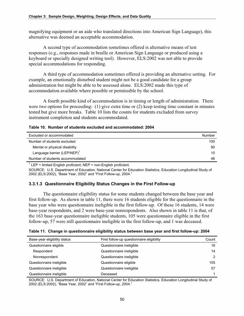
A fourth possible kind of accommodation is in timing or length of administration. There were two options for proceeding: (1) give extra time or (2) keep testing time constant in minutes tested but give more breaks. Table 10 lists the counts for students excluded from survey instrument completion and students accommodated.
Table 10. Number of students excluded and accommodated: 2004
Excluded or accommodated Number Number of students excluded 100
Mental or physical disability 90 Language barrier (LEP/NEP)1 10 Number of students accommodated 48 1 LEP = limited English proficient; NEP = non-English proficient. SOURCE: U.S. Department of Education, National Center for Education Statistics, Education Longitudinal Study of 2002 (ELS:2002), “Base Year, 2002” and “First Follow-up, 2004.”
3.3.1.3 Questionnaire Eligibility Status Changes in the First Follow-up
The questionnaire eligibility status for some students changed between the base year and first follow-up. As shown in table 11, there were 16 students eligible for the questionnaire in the base year who were questionnaire ineligible in the first follow-up. Of these 16 students, 14 were base-year respondents, and 2 were base-year nonrespondents. Also shown in table 11 is that, of the 163 base-year questionnaire ineligible students, 105 were questionnaire eligible in the first follow-up, 57 were still questionnaire ineligible in the first follow-up, and 1 was deceased.
Table 11. Change in questionnaire eligibility status between base year and first follow-up: 2004
Base-year eligibility status First follow-up questionnaire eligibility Count Questionnaire eligible Questionnaire ineligible 16 Respondent Questionnaire ineligible 14 Nonrespondent Questionnaire ineligible 2 Questionnaire ineligible Questionnaire eligible 105 Questionnaire ineligible Questionnaire ineligible 57 Questionnaire ineligible Deceased 1 SOURCE: U.S. Department of Education, National Center for Education Statistics, Education Longitudinal Study of 2002 (ELS:2002), “Base Year, 2002” and “First Follow-up, 2004.”
50

Chapter 3: Sample Design, Weighting, Design Effects, and Data Quality
3.3.1.4 Records and Contextual Data Gathered for Students Unable to be Surveyed or Validly Assessed
High school transcripts have been collected for students unable to be surveyed or validly assessed. School-level data, such as school administrator survey responses in the base year and first follow-up, have been linked to these students. Contextual or expanded sample cross-sectional and panel weights—as contrasted to the student questionnaire completion weights— have been created and are included on the restricted-use data file. See section 3.4 for a description of these weights and their uses.
3.3.2 Subsampling A base-year nonrespondent student was defined as a student that was selected in the base
year and did not complete a student questionnaire or portion of the questionnaire. Many of these students were enrolled in the same school during the follow-up. For the first follow-up, a subsample of 1,000 nonrespondent students was selected from the 2,229 base-year nonrespondents. Initially, a subsample of 1,620 nonrespondents was selected. All nonresponding students were included with certainty (i.e., probability equal to one), except for White students in public schools who were randomly subsampled. Then, to help the response rate and to conserve resources, the subsample of 1,620 was randomly subsampled across all student types to 1,000 nonrespondents. See table 12 for a summary of the nonrespondent subsample.
Table 12. Base-year nonrespondent subsample, by school sector and student type: 2004
Base-year School sector and student type nonrespondents Initial subsample Final subsample Public 1,843 1,234 764
1 All other races 1,006 397 246 Asian 289 289 179
Black or African American 286 286 177 Hispanic or Latino 262 262 162
Catholic 193 193 119 1 All other races 169 169 105
Asian 5 5 3 Black or African American 4 4 2
Hispanic or Latino 15 15 9
Other private 193 193 117 1 All other races 161 161 98
Asian 18 18 11 Black or African American 14 14 8
Hispanic or Latino # # # # Rounds to zero. 1 “All other races” includes White, American Indian or Alaska Native, Pacific Islander or Native Hawaiian, and Multiracial. All race categories exclude individuals of Hispanic or Latino origin. SOURCE: U.S. Department of Education, National Center for Education Statistics, Education Longitudinal Study of 2002 (ELS:2002), “Base Year, 2002” and “First Follow-up, 2004.”
51

Chapter 3: Sample Design, Weighting, Design Effects, and Data Quality
3.3.3 Student Sample Freshening Because part of the target population consists of those students who were enrolled in the
12th grade in the spring of 2004, the first follow-up included students at the base-year sample school who were enrolled in the 12th grade in the spring of 2004 but who were not in the 10th grade in the United States during the spring of 2002. During this time, such students may have been out of the country or may have been enrolled in school in the United States in a grade other than 10th (either at the sampled school or at some other school). In addition, some students may have reenrolled, although in spring 2002 they were temporarily out of school, owing to illness, injury, institutionalization, homeschooling, or school dropout.
Student freshening was limited to the base-year sample schools and the five new schools added due to school splits because all sample students were identified at these schools regardless of their status 2 years later, and they could be linked to potential freshened students. Freshened lists were not obtained from transfer schools. Therefore, a small number of freshening eligible students from “new” schools that were not on the 2002 school sampling frame did not have a chance of selection.
In October 2003, each sample school was asked to provide an electronic or hard copy listing of all their 12th-grade students enrolled in the 2003–04 school year. This requested listing was similar to the listing requested in the base year. The information requested for each eligible student included the following:
• student ID number; • Social Security number; • full name; • sex; and • race/ethnicity.
The race/ethnicity variable was used to stratify the students.
The sample school was given instructions for submitting the electronic and hardcopy lists. The electronic lists were requested to be a column formatted or comma delimited ASCII file or an Excel file. Schools were able to provide the electronic lists by sending them in an e-mail, providing a diskette or CD-ROM containing the file, or uploading the file to the ELS:2002 website. If the school could not provide an electronic list, then it was requested that the hardcopy lists were sorted in alphabetical order within race/ethnicity strata to facilitate stratified sampling. As shown in table 13, of the 615 enrollment lists received, 46.7 percent sent in electronic lists, 49.1 percent sent in hardcopy lists, and 4.2 percent sent in both types. The students from these 615 schools were selected such that the sample would be representative (i.e., linked to a representative sample of students in a representative sample of schools), as described in the following paragraphs. However, estimates based on respondents could potentially be biased due to nonresponse or excluding “new” schools. Nonresponse bias analysis was not conducted for the freshening nonresponse. However, nonresponse adjustment factors were computed to account for potential bias due to the school-level freshening nonresponse (see weighting section). Any bias due to excluding “new” schools is likely to be small due to the small number of freshening-eligible students. Approximately 130 schools did not send a
52

Chapter 3: Sample Design, Weighting, Design Effects, and Data Quality
freshened list, either because they refused to provide the list or because they indicated they had no freshening eligible students. Also, about 20 schools either sent in lists too late or sent lists that were incomplete and could not be used.
Table 13. Number of 12th-grade student lists provided by schools, by type: 2004
Type of list received Frequency1 Percent Total 615 100.00
Both electronic and hardcopy 26 4.23 Electronic copy 287 46.67 Hardcopy 302 49.11 1 The counts include all schools that sent in a 12th-grade student list, but three of these schools sent in a list that was not sufficient to use for freshening. SOURCE: U.S. Department of Education, National Center for Education Statistics, Education Longitudinal Study of 2002 (ELS:2002), “Base Year, 2002” and “First Follow-up, 2004.”
Quality assurance (QA) checks were performed on all lists received. Any list that was unreadable immediately failed the QA checks. Additionally, any list that did not allow the students to be stratified failed the QA checks, unless the original sophomore list also did not contain race/ethnicity. To verify that the school provided a complete list of eligible students, the school’s count of 12th-grade students from the most recent CCD (for public schools) and PSS (for private/Catholic schools) databases were compared with the counts (overall and within strata) of 12th-graders from the list provided. If any of the counts of 12th-graders for total students or by the race/ethnicity strata on the provided list were more than 25 percent lower or higher than the counts from the CCD data, then the list failed the QA checks, unless the provided count was greater than zero and the absolute difference was less than 50. However, if the provided count of Hispanics, Asians, or Blacks was zero and the original list count was less than five, the count did not fail the QA checks.
Table 14 shows that of the lists received, 512 passed all QA checks, 16 lists failed the QA check regarding student counts, 74 failed the QA check regarding identification of race stratum, 2 lists were unreadable, 4 lists had insufficient documentation, and 4 lists had multiple or other problems.
Table 14. Types of problems encountered with student lists: 2004
Type of problem Frequency Percent Total 612 100.00
None 512 83.66 Unreadable file or list 2 0.33 Count out of bounds 16 2.61 Cannot identify strata 74 12.09 Insufficient documentation 4 0.65 Multiple problems 1 0.16 Other problems 3 0.49 SOURCE: U.S. Department of Education, National Center for Education Statistics, Education Longitudinal Study of 2002 (ELS:2002), “Base Year, 2002” and “First Follow-up, 2004.”
53

Chapter 3: Sample Design, Weighting, Design Effects, and Data Quality
Schools that failed the QA checks were contacted to resolve the discrepancy. When it was determined that the initial list provided by the school was not satisfactory, a replacement list was requested. If the school confirmed that the provided list was correct or if the school sent a replacement list, then the freshening process was initiated. If the school refused to send a replacement list, then the freshening process was initiated, when possible.
If both the original and new enrollment lists were electronic, they were sorted alphabetically within stratum (as the original list was sorted for sample selection) to facilitate the comparison of the original and new lists. If one of the lists was electronic and one was hard copy, then the electronic list was sorted alphabetically within stratum and printed for the freshening process. If both of the lists were hard copy, then the lists were used as is in the freshening process.
The freshening process began by identifying the base-year sample students on the new list. If the student immediately following each sampled base-year student within the race/ethnicity strata on the new list was not on the original list, then that student was selected as a potential addition to the sample. Whenever a potential new sample student was identified, the next student on the list was examined to determine whether that student was on the original list. If this next student was not on the original list, then that student was a potential addition to the sample. This process was continued until reaching a student who was on the original list. Then, this process was repeated with the next base-year sample student on the list.22
Next, the school was contacted to determine the eligibility of the freshened students. Any student identified as eligible by the school was selected into the sample.
Table 15 shows that 2,712 freshened students were included in the first follow-up sample. Of these 2,712 students, 238 (8.8 percent) were found to be eligible for inclusion in the study, and 2,474 students (91.2 percent) were found to be ineligible. Of the 238 eligible freshened students, 31 were questionnaire ineligible. Eligibility was determined for all freshened students. The high ineligibility rate was expected because the freshening procedure selected 12th-grade students who were not on the sophomore list without information on their status in the 10th grade. Many of these sampled students were sophomores at other regular U.S. schools in the spring of 2002 who transferred to a sample school, which contributed to the high ineligibility rate. The number of freshened students was approximately 0.39 students per school (238 students out of 612 schools that sent usable 12th-grade enrollment lists).
Table 15. Number of freshened sample members, by eligibility: 2004
Freshened eligibility status Count Percent Total 2,712 100.00
Eligible 207 7.63 Questionnaire ineligible 31 1.14 Ineligible 2,474 91.22 SOURCE: U.S. Department of Education, National Center for Education Statistics, Education Longitudinal Study of 2002 (ELS:2002), “Base Year, 2002” and “First Follow-up, 2004.”
22 This process is also known as the half-open interval rule.
54

Chapter 3: Sample Design, Weighting, Design Effects, and Data Quality
3.4 Calculation of Weights and Results of Weighting
3.4.1 Analysis Populations The sample design for ELS:2002 supports a number of analyses, which in turn permit
accurate inferences to be made to three major groups or target populations. Within these populations are important analytical domains.
Population A: Spring 2002 sophomores
Domains:
• spring 2002 sophomores capable of completing the student questionnaire
• all spring 2002 sophomores including those capable and not capable of completing the questionnaire
• spring 2002 sophomores in base-year school in spring 2004
• spring 2002 sophomores in a different school in spring 2004 (transfers)
• spring 2002 sophomores who were dropouts in spring 2004
• spring 2002 sophomores who graduated or achieved equivalency early, that is, prior to March 15, 2004
• spring 2002 sophomores who were homeschooled in spring 200423
• spring 2002 White sophomores
• spring 2002 Black sophomores
• spring 2002 Hispanic sophomores
• spring 2002 Asian sophomores
• spring 2002 public school sophomores
• spring 2002 private school sophomores
Population B: Spring 2004 12th-grade students
Domains:
• spring 2004 12th-grade students capable of completing the student questionnaire
• all spring 2004 12th-grade students including those capable and not capable of completing the questionnaire
• spring 2004 12th-grade students who were graduating high school seniors in spring 2004
23 Although conceptually spring 2002 sophomores who were homeschooled in 2004 may be thought of as an analysis population, they were not designed to be so and were therefore not subject to minimum sample size requirements. The group is of limited analytic utility owing both to the low sample size and to the narrowness of the population definition. The compelling practical reason for distinguishing this group was so that they could be administered only those items consonant with their unique situation as out-of-school students.
55

Chapter 3: Sample Design, Weighting, Design Effects, and Data Quality
• spring 2004 White 12th-grade students
• spring 2004 Black 12th-grade students
• spring 2004 Hispanic 12th-grade students
• spring 2004 Asian 12th-grade students
• spring 2004 public school 12th-grade students
• spring 2004 private school 12th-grade students
Figure 2 helps illustrate that, whereas some students are in only population A or population B, many students are in both populations—that is, both a spring 2002 sophomore and a spring 2004 12th-grade student. Figure 3 further illustrates the overlap between the two populations.
Figure 2. Student analysis populations, by year: 2004
SOURCE: U.S. Department of Education, National Center for Education Statistics, Education Longitudinal Study of 2002 (ELS:2002), “Base Year, 2002” and “First Follow-up, 2004.”
56

Figure 3. Student analysis population respondent counts, by year: 2004
Number of respondents
14,000
12,000
10,000
8,000
6,000
4,000
2,000
0
A: Spring 2002 10th-grade students B: Spring 2004 12th-grade students
1,579
202
13,308
A, Not B B, Not A Both A and B
Population
Chapter 3: Sample Design, Weighting, Design Effects, and Data Quality
SOURCE: U.S. Department of Education, National Center for Education Statistics, Education Longitudinal Study of 2002 (ELS:2002), “Base Year, 2002” and “First Follow-up, 2004.”
Population C: Spring 2002 10th-grade schools
Domains:
• control
• urbanicity
• region
Analytic uses of these three populations, and the weighting required to support the analyses, are discussed in sections 3.4.2 (student level) and 3.4.3 (school level).
3.4.2 Uses of Student-Level Data; Student Weights 3.4.2.1 Population A: Spring 2002 Sophomores
This population can be employed in both cross-sectional and longitudinal analyses. (Note to the user: The expanded weights [BYEXPWT and F1XPNLWT] are only available on the restricted-use file.) Weights for cross-sectional analyses were created in the base year. BYSTUWT can be used for cross-cohort comparisons of students capable of completing the questionnaire (on an intercohort time-lag basis employing the sophomore classes of 1980 and 1990). BYEXPWT generalizes to the entire population, including both students capable and incapable of completing the questionnaire.
57

Chapter 3: Sample Design, Weighting, Design Effects, and Data Quality
The weight F1PNLWT was created for all persons who completed a questionnaire or a sufficient portion of a questionnaire, both in the base year and the first follow-up. Also, base-year data were imputed when not available from the new participant supplement (NPS) for first follow-up respondents, and these cases also have F1PNLWT. The panel weight can be used for both intracohort (across rounds of ELS:2002) and intercohort (longitudinal comparative analysis) purposes. An example of using a panel weight for intracohort analysis is to take a cohort of sophomores, look at their enrollment 2 years later, and determine what proportion have dropped out. An example of using a panel weight for intercohort analysis is to compute math gains between sophomore and senior years using the ELS:2002 panel weight and also for the NELS:88 panel weight and then comparing the gain between sophomore and senior year for the two cohorts. Missing test data were imputed, so a version of the panel weight adjusted for test nonresponse was unnecessary. The weight F1XPNLWT was created for the expanded sample of students capable and not capable of completing the questionnaire. See section 3.4.4 for more details.
Base-year nonrespondents who responded in the first follow-up are considered to be part of this population, but there is no base-year weight (BYSTUWT or BYEXPWT) for them. The NPS ensured that the standard classification variables collected in the base year were also available for this group. However, key variables were imputed for base-year nonrespondents who were first follow-up respondents (see section 3.6), so that these students could be analyzed as part of the sophomore panel using F1PNLWT and/or F1XPNLWT. BYSTUWT and BYEXPWT were not recomputed.
Transcripts will provide continuous data covering grades 9 through 12 for students who remained in school and were in the modal grade sequence (or a lesser range of data for students who dropped out or fell behind the modal progression). A cross-sectional 2004 transcript weight (F1TRSCWT) will be produced, encompassing cases that meet the following conditions, for sample members for whom a transcript has been obtained: (a) member of the 10th-grade or the 12th-grade cohort who was a student questionnaire completer in the base year, first follow-up, or both; or (b) member of the questionnaire-incapable expanded sample. This weight will generalize to the analysis population of spring 2002 sophomores by subsetting the sample through the use of a flag (G10COHRT). In addition, a transcript panel weight (F1TRPWT) will be produced for all individuals who have a transcript in 2004 and who are regular or expanded sample participants in both 2002 and 2004, including base-year nonrespondents with imputed data. See section 3.4.4 for more details.
3.4.2.2 Population B: Spring 2004 12th-Grade Students
This population can also be employed in both cross-sectional and longitudinal analyses. (Note to the user: The expanded weight [F1EXPWT] is only available on the restricted-use file.) The longitudinal analyses will be conducted after further rounds of the study. Weights for cross-sectional (including cross-cohort) analyses (F1QWT) were created for students capable of completing the questionnaire. This weight should be used in conjunction with a flag (G12COHRT) that identifies the sample member as part of the senior cohort. F1EXPWT will generalize to the entire population, including students capable and incapable of completing the questionnaire. See section 3.4.4 for more details.
58

Chapter 3: Sample Design, Weighting, Design Effects, and Data Quality
Note that generalizations about the mathematics achievement of the 2004 senior class involve imputation for the transfer students and other seniors who were not tested (see section 3.6).
The cross-sectional transcript weight described above will also generalize to the analysis population of spring 2004 12th-graders by subsetting the sample through the use of a flag (G12COHRT). See section 3.4.4 for more details.
3.4.3 Uses of School-Level Data; School-Level Weights This population of spring 2002 10th-grade schools can be employed in cross-sectional
analyses and potentially in longitudinal analyses. Weights for cross-sectional analyses were created in the base year. BYSCHWT can be used for spring 2002 10th-grade schools.
The first follow-up school data can be analyzed using the student weight. That is, the school data can be analyzed in relation to student characteristics (i.e., the administrator data are linked to student data, with the student as the fundamental unit of analysis).
Although it is not possible to produce a cross-sectional 2004 school weight because the first follow-up school sample is not nationally representative of American high schools in 2004, the base-year school weight can be used for longitudinal analyses treating the base-year schools as a panel. Although there are multiple data points for analysis, the weight maintains generalizability only to schools in 2002.
3.4.4 Weights Four sets of weights were computed:
• A cross-sectional weight for the expanded sample that includes sample numbers who completed all or a sufficient portion of the questionnaire in the first follow-up, the base-year students who were still incapable of completing the questionnaire 2 years later, base-year students who were newly incapable of completing the questionnaire, and freshened students who were incapable of completing the questionnaire (F1EXPWT). This weight is only available on the restricted-use file.
• A cross-sectional first follow-up weight for sample members who completed all or a sufficient portion of the questionnaire in the first follow-up (F1QWT).
• A first follow-up panel weight (longitudinal weight) for the expanded sample that includes students who fully or partially completed a questionnaire in both the base year and first follow-up, students who fully or partially completed a questionnaire in the first follow-up and had base-year data imputed if not on the NPS (see section 3.6), and students who were questionnaire incapable in the base year and/or the first follow-up (F1XPNLWT). This expanded sample panel weight is only available on the restricted-use file.
• A first follow-up panel weight for sample members who fully or partially completed a questionnaire in both the base year and first follow-up or who fully or partially
59

Chapter 3: Sample Design, Weighting, Design Effects, and Data Quality
completed a questionnaire in the first follow-up and had base-year data imputed if not on the NPS (F1PNLWT).
Also, two weights (only available on the restricted-use file) will be computed and documented later:
• a cross-sectional transcript weight for sample members for whom transcript data have been collected and who either fully or partially completed a questionnaire in the first follow-up or were members of the expanded sample (F1TRSCWT); and
• a panel transcript weight for sample members for whom transcript data have been collected and who either fully or partially completed a questionnaire in both the base year and first follow-up, fully or partially completed a questionnaire in the first follow-up and had base-year data imputed if not on the NPS, or were members of the expanded sample (F1TRPWT).
Additionally, there are two flags that can be used in analyses to identify members of the sophomore and senior cohorts:
• a flag indicating a member of the sophomore cohort, that is, spring 2002 sophomore (G10COHRT); and
• a flag indicating a member of the senior cohort, that is, spring 2004 12th-grader (G12COHRT).
Table 16 illustrates the relationship among the first four weights listed above plus the base-year weights, universe flags, populations described in section 3.4.1, and respondents. Below, the weighting procedures are described for the first four of these weights. The procedures for calculating F1QWT differ somewhat for base-year sample students and first follow-up freshened sample students.
3.4.4.1 F1EXPWT for Base-Year Sample Students
The expanded sample cross-sectional weight was computed for the expanded sample that includes students who fully or partially completed the questionnaire and students incapable of completing the questionnaire.24 In addition to the expanded sample students identified in the base year, such students could be those who were base-year nonrespondents, became disabled between the base year and first follow-up, or were misclassified in the base year.
With a few exceptions, base-year eligible sample students remained eligible for the first follow-up sample. Students who died were out of scope for the first follow-up. Students who left the country, were unavailable for the duration of the study (e.g., in military boot camp), or were institutionalized were temporarily out of scope for the first follow-up, although they may be eligible in future rounds.
24 The expanded sample weights and the full expanded sample are available on the restricted-use file but not on the public-use file.
60

Chapter 3: Sample Design, Weighting, Design Effects, and Data Quality
Table 16. Relationship among weights, populations, respondents, and universe flags: 2004
Weight1 Universe flag Population Respondent BYSTUWT G10COHRT Spring 2002
sophomore Fully or partially completed questionnaire in 2002
BYEXPWT G10COHRT Spring 2002 sophomore
Fully or partially completed questionnaire in 2002 or incapable of completing a questionnaire
F1PNLWT G10COHRT Spring 2002 sophomore
Fully or partially completed questionnaire in 2002 and 2004 (base-year data may be imputed)
F1XPNLWT G10COHRT Spring 2002 sophomore
Fully or partially completed questionnaire in 2002 and 2004 (base-year data may be imputed) or incapable of completing a questionnaire in 2002 or 2004
F1QWT G10COHRT Spring 2002 sophomore
Fully or partially completed questionnaire in 2004
G12COHRT Spring 2004 12th-grader
F1EXPWT G10COHRT Spring 2002 sophomore
Fully or partially completed questionnaire in 2004 or incapable of completing a questionnaire in 2004
G12COHRT Spring 2004 12th-grader
1 The expanded sample weights and the full expanded sample are available on the restricted-use file but not on the public-use file. SOURCE: U.S. Department of Education, National Center for Education Statistics, Education Longitudinal Study of 2002 (ELS:2002), “Base Year, 2002” and “First Follow-up, 2004.”
First, the student-level design weight (F1DWT) was calculated as equal to the base-year design weight multiplied by the reciprocal of the student’s probability to be included in the first follow-up. All base-year eligible sample students have a base-year design weight (BYDWT) that accounts for the base-year school probability of selection (adjusted for nonresponse) and for the base-year student probability of selection within the sample school. This base-year design weight is not adjusted for base-year student nonresponse. The student’s probability of selection in the first follow-up is 1.0 for base-year respondents and base-year questionnaire-incapable students and less than 1.0 for base-year nonrespondents. This weight is used because all base-year respondents are in the first follow-up sample, and 1,000 out of 2,229 base-year nonrespondents were subsampled to be included in the first follow-up sample. Different subsampling rates were used for the various school types and student types. Note that hostile refusals—those who requested to be removed from the study for all rounds—had a positive probability of selection but were always treated as first follow-up nonrespondents. The formula for F1DWT for student i is
F1DWTi = BYDWTi * (1 / P1i),
where P1i is the probability of selection for student i for the first follow-up sample.
In the base year, all nonresponding students were assumed to be eligible. Adjusting the weights of base-year nonrespondents to compensate for the small portion of students who were actually ineligible was considered. However, in CATI, only nine ineligible students were identified, so it was assumed that all of the nonrespondents were eligible. If the assumption was made that some nonrespondents were ineligible, the adjustment would be negligible. In the first
61

Chapter 3: Sample Design, Weighting, Design Effects, and Data Quality
follow-up, some of these nonrespondents still had unknown eligibility, including some for whom the name was unknown. Again, they were assumed to be eligible, as they were in the base year.
Next, generalized exponential models (GEM) (Folsom and Singh 2000) were used. The GEM approach is a general version of weighting adjustments and was based on a generalization of Deville and Särndal’s logit model (Deville and Särndal 1992). GEM is not a competing method to weighting classes or logistic regression; rather, it is a method employed to do weight adjustments with a choice of optional features to employ. It is a formalization of weighting procedures such as nonresponse adjustment, poststratification, and weight trimming. GEM controls at the margins as opposed to controlling at the cell level, as weighting class adjustments. This approach allows more variables to be considered. GEM is designed so that the sum of the unadjusted weights for all eligible units equals the sum of the adjusted weights for respondents. GEM also constrains the nonresponse adjustment factors to be greater than or equal to one.
The questionnaire-incapable students are generally included as part of the expanded set of cases, but a small number of hostile refusals were treated as nonrespondents. Therefore, a simple weighting class nonresponse adjustment was performed. The classes were formed by school type, given the small number of questionnaire-ineligible students. This nonresponse adjustment factor is WTADJ1, and these students have a second nonresponse adjustment factor (WTADJ2) equal to one (see below). For questionnaire-capable students, a first follow-up respondent is defined as a student who completed the questionnaire or a significant portion of the questionnaire. The variables used in the nonresponse weight adjustment were those available for most respondents and nonrespondents that are described in section 3.8.
The student nonresponse was performed in two stages—refusal and other nonresponse— because the predictors of response propensity were potentially different at each stage. The nonresponse models reduce the bias due to nonresponse for the model predictor variables and related variables. Therefore, using these two stages of nonresponse adjustment achieved greater reduction in nonresponse bias to the extent that different variables were significant predictors of response propensity at each stage.
For data known for most but not all students, data collected from responding students and weighted hot deck imputation were used so that data are available for all eligible sample students. These variables were main effects in the models. They were also used in Automatic Interaction Detection (AID) analyses (with response as the dependent variable) to determine important interactions for the nonresponse adjustment models. The outcomes of these first models were nonresponse adjustment factors (WTADJ1 and WTADJ2). The unequal weighting effects (UWEs) and maximum adjustment factors were monitored to ensure reasonable values.
Next, the GEM approach was used to poststratify the nonresponse adjusted weights— that is, F1DWT * WTADJ1 * WTADJ2—to meet overall and marginal totals of the base-year expanded sample weights (BYEXPWT). The full expanded sample was included in this adjustment, and the control totals were the base-year expanded weight sums, because students can potentially move in and out of being questionnaire incapable (i.e., being questionnaire capable or questionnaire incapable is not static). The variables used in poststratification were school type and student race/ethnicity. This adjustment ensures that the first follow-up weight
62

Chapter 3: Sample Design, Weighting, Design Effects, and Data Quality
sums are equal to the base-year weight sums for these variables. GEM generated a poststratification adjustment factor (WTADJ3).
Extreme weights occur in the ELS:2002 data due to small probabilities of sample selection or due to weight adjustments. These extreme weights (either very small or very large) can significantly increase the variance of estimates. One way to account for this and decrease the variance is to trim and smooth extreme weights within prespecified domains. Note that trimming weights has the potential to increase bias. However, the increase in bias is often offset by the decrease in variance due to weight trimming. As a result, this reduces the mean square error (MSE) of an estimate, defined as variance plus bias squared.
The innovation introduced in GEM is the ability to incorporate specific lower and upper bounds. An important application of this feature is to identify at each adjustment step an initial set of cases with extreme weights and to use specific bounds to exercise control over the final adjusted weights. Thus, there is built-in control for extreme weights in GEM.
GEM uses the median +/– X * IQR, where X is any number, typically between 2 and 3, and IQR is the interquartile range. There are also different points in the weight adjustment process during which weight trimming can occur. GEM has options to make adjustments for extreme weights as part of the nonresponse and as part of the poststratification. GEM adjusted for ELS:2002 extreme weights during both nonresponse adjustments, as well as during the poststratification. For GEM, a variable or set of variables is identified to be used to identify extreme weights within each level of the variable(s), and the variables race and school type were chosen. Prior to running GEM, the unweighted and weighted percentage of extreme weights was examined for all four levels of race crossed with the three levels of school type using various values to multiply by the IQR (2.0, 2.1, 2.2,…4.0), and the value of 2.5 was chosen.
The final student weight for the expanded sample student i is the product of the first follow-up design weight, the nonresponse adjustment factors, and the poststratification factor, such that
F1EXPWTi = F1DWTi * WTADJ1i * WTADJ2i * WTADJ3i.
3.4.4.2 F1EXPWT for First Follow-up Freshened Sample Students
The expanded sample cross-sectional weight was computed for eligible freshened sample students who fully or partially completed the questionnaire or who were incapable of completing the questionnaire. These sample students were not in the base-year population (i.e., not in 10th grade in the United States in spring 2002). During 2002, such students may have been out of the country, been enrolled in school in the United States in a grade other than 10th, had an extended illness or injury, been institutionalized, been homeschooled, or temporarily dropped out of school. A 12th-grade enrollment list was requested from each base-year school or from the new school if the base-year school was closed, split, or did not enroll 12th-graders. Students were identified who were on the 12th-grade enrollment list but not on the sophomore list. Each of these students was linked to a student on the sophomore enrollment list, and they were selected for the freshened sample if the linked sophomore had been selected for the base-year sample.
63

Chapter 3: Sample Design, Weighting, Design Effects, and Data Quality
The first follow-up design weight (F1DWT) for each freshened sample student is therefore equal to the base-year design weight of the linked sophomore.
After the freshened sample students were selected, the schools were asked to identify those that were eligible for freshening (i.e., those that were not in the base-year population). Of 2,702 sampled freshened students, 425 (16 percent) were determined by the school to be eligible. Freshened eligibility was determined by the school for all freshened students. However, more than 150 of these freshened students determined by the school to be eligible were later determined during the student interview to be ineligible. There were no nonresponding freshened students with undetermined eligibility.
In the first follow-up, 612 schools sent a 12th-grade enrollment list that was sufficient for selecting freshened students. This number includes new schools that were added as a result of base-year schools that split. Another 13 schools did not send a 12th-grade enrollment list because they either did not have any 12th-graders that were new to the school since spring 2002 or they did not enroll 12th-graders. Therefore, 127 of the 752 base-year participating schools did not provide a freshened list.
The freshened student weights were adjusted upward to account for the school nonresponse to freshening. Weighting classes were formed from the variables school type and school metropolitan status. Each class had a minimum of 30 eligible freshened students. First, the average number of eligible freshened students per school that sent in a 12th-grade list was calculated. Next, this average was multiplied by the number of schools that did not send in a list. Then, this number was added to the eligible freshened students, and this sum was divided by the number of eligible freshened students. The result is the weight adjustment factor WTADJ1j for weighting class j:
WTADJ1j = ((Avgj * NRj) + FEj) / FEj,
where:
Avgj is the average number of eligible freshened students per school that sent in a 12th-grade list in weighting class j;
NRj is the number of schools in weighting class j that did not respond to the request to send in a 12th-grade list; and
FEj is the number of eligible freshened students in weighting class j.
The nonresponse adjustment for the freshened sample students was done together with the nonresponse adjustment for the base-year sample students because of the small number of eligible freshened students. A flag for freshened students was included in the nonresponse models. The outcomes of the nonresponse models were nonresponse adjustment factors (WTADJ2 and WTADJ3).
64

Chapter 3: Sample Design, Weighting, Design Effects, and Data Quality
Table 17 presents the final predictor variables used in the first-stage student nonresponse adjustment model, which includes both base-year and freshened sample students. This table also includes the average weight adjustment factors resulting from these variables: 3.73 percent unweighted and 14.30 percent weighted of the students were identified as having extreme weights. The first stage of nonresponse adjustment factors met the following constraints:
• minimum: 0.10
• median: 1.08
• maximum: 2.12
Table 18 presents the final predictor variables used in the second-stage student nonresponse adjustment model, which includes both base-year and freshened sample students. This table includes the average weight adjustment factors resulting from these variables: 3.13 percent unweighted and 8.93 percent weighted of the students were identified as having extreme weights. The second stage of nonresponse adjustment factors met the following constraints:
• minimum: 0.09 • median: 1.05 • maximum: 2.35
Table 17. Average weight adjustment factors used to adjust cross-sectional weights for refusal, by selected characteristics: 2004
Model predictor variables1
Total
Number of responding students and “other”
nonresponding students2
15,608
Weighted response
rate 94.97
Average weight
adjustment factor
1.11
School sector Public Catholic Other private
12,262 1,929 1,417
95.07 94.63 92.89
1.11 1.07 1.20
School urbanicity Urban Suburban Rural
5,325 7,449 2,834
94.56 94.79 96.05
1.13 1.10 1.09
10th-grade enrollment 0–99 100–249 250–499
≥ 500 See notes at end of table.
3,033 3,971 4,992 3,612
96.26 95.71 94.69 94.22
1.11 1.08 1.12 1.12
65

Chapter 3: Sample Design, Weighting, Design Effects, and Data Quality
Table 17. Average weight adjustment factors used to adjust cross-sectional weights for refusal, by selected characteristics: 2004—Continued
Number of responding students Average
and “other” Weighted weight
Model predictor variables1 nonresponding
students2 response
rate adjustment
factor Type of grades within school K–12, PreK–10th, 1st–12th, PreK/1st–9th/12th and PreK–12
schools 1,021 95.97 1.21 Middle grades but no elementary 1,638 95.14 1.08
Only high school 12,949 94.90 1.10
Number of grades within the school 4 11,906 95.03 1.10 > or < 4 3,702 94.73 1.13
Number of days in school year Less than 180 days 4,055 95.49 1.10
180 days 8,642 95.10 1.11 More than 180 days 2,911 93.88 1.13
Minutes per class period ≤ 45 3,733 94.65 1.11
46–50 3,346 94.59 1.11 51–80 4,168 94.85 1.13
≥ 81 4,361 95.56 1.09
Class periods per day 1–4 4,504 95.60 1.09 5–6 3,849 94.33 1.12
7 4,215 94.63 1.11 8–9 3,040 95.33 1.11
IEP3 percentage ≤ 5 percent 6,042 94.77 1.11
6–10 percent 4,023 94.88 1.10 11–15 percent 3,450 95.29 1.10
> 15 percent 2,093 94.93 1.14
LEP4 percentage 0 percent 6,722 95.73 1.10 1 percent 3,053 94.24 1.11 2–5 percent 2,631 94.44 1.11
≥ 6 percent 3,202 95.01 1.13 See notes at end of table.
66

Chapter 3: Sample Design, Weighting, Design Effects, and Data Quality
Table 17. Average weight adjustment factors used to adjust cross-sectional weights for refusal, by selected characteristics: 2004—Continued
Number of responding students Average
and “other” Weighted weight
Model predictor variables1 nonresponding
students2 response
rate adjustment
factor Free or reduced-price lunch
0 percent 2,753 92.89 1.11 1–10 percent 3,484 93.72 1.12 11–30 percent 4,693 95.45 1.11 ≥ 31 percent 4,678 95.95 1.09
Number of full-time teachers 1–40 4,033 96.00 1.09 41–70 3,938 95.13 1.09 71–100 4,038 94.70 1.13 > 100 3,599 94.48 1.12
Number of part-time teachers 0–1 4,545 95.17 1.10 2–3 4,467 95.48 1.11 4–6 3,768 94.11 1.12
≥ 7 2,828 94.85 1.11
Full-time teachers certified 0–90 percent 4,016 95.63 1.11 91–99 percent 2,755 94.46 1.11 100 percent 8,837 94.97 1.11
School coeducational status Coeducational school 14,814 95.00 1.11 All-female school 366 91.82 1.08 All-male school 428 95.08 1.06
Total enrollment 0–600 students 3,672 96.45 1.09 601–1,200 students 4,652 94.68 1.11 1,201–1,800 students 3,563 94.70 1.10 > 1,800 students 3,721 94.59 1.13 See notes at end of table.
67

Chapter 3: Sample Design, Weighting, Design Effects, and Data Quality
Table 17. Average weight adjustment factors used to adjust cross-sectional weights for refusal, by selected characteristics: 2004—Continued
Number of responding students Average
and “other” Weighted weight
Model predictor variables1 nonresponding
students2 response
rate adjustment
factor Census region
Northeast 2,881 94.65 1.12 Midwest 3,903 95.04 1.10 South 5,629 95.79 1.08 West 3,195 93.94 1.16
All other races 10th-grade enrollment ≤ 80 percent 7,821 95.09 1.11 > 80 percent 7,787 94.84 1.11
Asian 10th-grade enrollment ≤ 2 percent 6,034 95.25 1.09 > 2 percent 9,574 94.80 1.12
Black or African American 10th-grade enrollment ≤ 4 percent 5,279 94.50 1.11 > 4 percent 10,329 95.21 1.11
Hispanic or Latino 10th-grade enrollment ≤ 3 percent 5,993 94.63 1.10 > 3 percent 9,615 95.17 1.11
CHAID5 segments CHAID segment 1 = 1–40 full-time teachers; public school;
≤ 2 percent Asian 10th-grade enrollment 1,323 94.41 1.12 CHAID segment 2 = 1–40 full-time teachers; public school;
> 2 percent Asian 10th-grade enrollment 405 87.90 1.15 CHAID segment 3 = 1–40 full-time teachers; Catholic and
other private schools; race = Hispanic or other 751 96.00 1.09 CHAID segment 4 = 1–40 full-time teachers; Catholic and
other private schools; race = Asian or Black 1,119 94.26 1.10 CHAID segment 5 = 41–70 full-time teachers; 0–6 part-time
teachers; 1–6 class periods 599 90.59 1.16 CHAID segment 6 = 41–70 full-time teachers; 0–6 part-time
teachers; 7–9 class periods 1,055 94.61 1.11 CHAID segment 7 = 41–70 full-time teachers; ≥ 7 part-time
teachers; ≤ 180 school days 985 92.90 1.15 CHAID segment 8 = 41–70 full-time teachers; ≥ 7 part-time
teachers; > 180 school days 1,052 98.62 1.07 See notes at end of table.
68

Chapter 3: Sample Design, Weighting, Design Effects, and Data Quality
Table 17. Average weight adjustment factors used to adjust cross-sectional weights for refusal, by selected characteristics: 2004—Continued
Number of responding students Average
and “other” Weighted weight
Model predictor variables1 nonresponding
students2 response
rate adjustment
factor CHAID5 segments—Continued
CHAID segment 9 = > 70 full-time teachers; 0–1 part-time teachers; ≤ 80 percent other 10th-grade enrollment 1,747 97.40 1.05
CHAID segment 10 = > 70 full-time teachers; 0–1 part-time teachers; > 80 percent other 10th-grade enrollment 2,546 96.47 1.10
CHAID segment 11 = > 70 full-time teachers; ≥ 2 part-time teachers; ≤ 45 minutes per class 1,966 95.18 1.11
CHAID segment 12 = > 70 full-time teachers; ≥ 2 part-time teachers; 46–80 minutes per class 197 98.37 1.15
CHAID segment 13 = > 70 full-time teachers; ≥ 2 part-time teachers; ≥ 81 minutes per class 645 91.04 1.16
CHAID segment 14 = 11+ percent free or reduced-price lunch; in-school out-of-grade enrollment status; 1,801+ total enrollment 526 95.86 1.14
CHAID segment 15 = 11+ percent free or reduced-price lunch; out-of-school enrollment status; race = Asian,
White, or other 325 86.98 1.21 CHAID segment 16 = 11+ percent free or reduced-price
lunch; out-of-school enrollment status; race = Black, Hispanic, Indian, or Pacific Islander 367 94.06 1.10
Sex Male 7,811 95.16 1.11 Female 7,797 94.77 1.10
Race/ethnicity6
All other races 9,517 94.56 1.13 Asian 1,744 94.80 1.09 Black or African American 2,345 95.88 1.08 Hispanic or Latino 2,002 95.90 1.06
Freshened status
Freshened 186 88.75 1.16
Enrollment status In school, in grade (in grade 12) 12,842 95.67 1.10 In school, out of grade (in grade 10 or 11, ungraded, or
graduated early) 1,892 93.33 1.15 Out of school (dropout or homeschooled) 874 90.20 1.17
See notes at end of table.
69

Chapter 3: Sample Design, Weighting, Design Effects, and Data Quality
Table 17. Average weight adjustment factors used to adjust cross-sectional weights for refusal, by selected characteristics: 2004—Continued
Number of responding students Average
and “other” Weighted weight
Model predictor variables1 nonresponding
students2 response
rate adjustment
factor School sector and race/ethnicity
Public schools, All other races 6,882 94.68 1.13 Public schools, Asian 1,589 94.59 1.10
Public schools, Black or African American 2,076 95.96 1.07 Public schools, Hispanic or Latino 1,715 95.89 1.07 Catholic schools, All other races 1,464 94.77 1.07 Catholic schools, Asian 77 98.06 1.02
Catholic schools, Black or African American 175 92.37 1.09 Catholic schools, Hispanic or Latino 213 93.85 1.02
Other private school, All other races 1,171 91.86 1.21 Other private schools, Asian 78 96.49 1.04
Other private schools, Black or African American 94 94.35 1.30 Other private schools, Hispanic or Latino 74 98.37 1.01
1 Model predictor variables had a value of 0 or 1. Some of the listed model predictor variables were not actually in the model because they served as reference groups. For each group of variables, one of the categories (predictor variable) was used as a reference group. 2 “Other” nonresponding students are students who were nonrespondents but did not explicitly refuse. Responding students are grouped with the “other” nonrespondents for the first nonresponse adjustment that adjusts for refusals. 3 IEP = Individualized Education Program. 4 LEP = limited English proficient. 5 CHAID = chi-squared automatic interaction detection. 6 “All other races” includes White, American Indian or Alaska Native, Pacific Islander or Native Hawaiian, and Multiracial. All race categories exclude individuals of Hispanic or Latino origin. SOURCE: U.S. Department of Education, National Center for Education Statistics, Education Longitudinal Study of 2002 (ELS:2002), “Base Year, 2002” and “First Follow-up, 2004.”
70

Chapter 3: Sample Design, Weighting, Design Effects, and Data Quality
Table 18. Average weight adjustment factors used to adjust cross-sectional weights for other nonresponse, by selected characteristics: 2004
Average Number of Weighted weight
Model predictor variables1 responding
students response
rate adjustment
factor Total 14,884 94.83 1.06
School sector Public 11,604 94.63 1.07 Catholic 1,899 98.69 1.02 Other private 1,381 95.38 1.06
School urbanicity Urban 5,020 93.12 1.08 Suburban 7,140 95.42 1.06 Rural 2,724 95.98 1.05
10th-grade enrollment 0–99 2,922 95.77 1.06 100–249 3,847 96.45 1.04 250–499 4,760 95.01 1.07
≥ 500 3,355 93.00 1.09
Type of grades within school K–12, PreK–10th, 1st–12th, PreK/1st–9th/12th and PreK–12 schools 995 96.05 1.06 Middle grades but no elementary 1,570 95.29 1.05
Only high school 12,319 94.72 1.07
Number of grades within the school 4 11,330 94.72 1.07 > or < 4 3,554 95.28 1.06
Number of days in school year Less than 180 days 3,897 95.24 1.05
180 days 8,228 94.74 1.07 More than 180 days 2,759 94.58 1.07
Minutes per class period ≤ 45 3,574 95.12 1.06
46–50 3,203 95.52 1.06 51–80 3,970 94.65 1.07
≥ 81 4,137 94.33 1.07 See notes at end of table.
71

Chapter 3: Sample Design, Weighting, Design Effects, and Data Quality
Table 18. Average weight adjustment factors used to adjust cross-sectional weights for other nonresponse, by selected characteristics: 2004—Continued
Average Number of Weighted weight
Model predictor variables1 responding
students response
rate adjustment
factor Class periods per day 1–4 4,277 94.59 1.07 5–6 3,654 94.66 1.07
7 4,029 94.65 1.06 8–9 2,924 95.80 1.06
IEP2 percentage ≤ 5 percent 5,848 95.76 1.05
6–10 percent 3,811 94.64 1.07 11–15 percent 3,260 94.52 1.08
> 15 percent 1,965 94.12 1.09
LEP3 percentage 0 percent 6,501 96.08 1.05 1 percent 2,932 95.96 1.05 2–5 percent 2,476 93.57 1.08
≥ 6 percent 2,975 92.99 1.09
Free or reduced-price lunch 0 percent 2,691 97.07 1.04 1–10 percent 3,372 96.46 1.05 11–30 percent 4,447 94.61 1.07
≥ 31 percent 4,374 93.27 1.09
Number of full-time teachers 1–40 3,886 96.16 1.05 41–70 3,812 96.56 1.05 71–100 3,810 94.16 1.08 > 100 3,376 93.29 1.08
Number of part-time teachers 0–1 4,273 93.69 1.07 2–3 4,287 95.35 1.06 4–6 3,608 95.22 1.06
≥ 7 2,716 95.54 1.06 See notes at end of table.
72

Chapter 3: Sample Design, Weighting, Design Effects, and Data Quality
Table 18. Average weight adjustment factors used to adjust cross-sectional weights for other nonresponse, by selected characteristics: 2004—Continued
Average Number of Weighted weight
Model predictor variables1 responding
students response
rate adjustment
factor Full-time teachers certified 0–90 percent 3,846 94.32 1.06 91–99 percent 2,606 93.92 1.08 100 percent 8,432 95.26 1.06
School coeducational status Coeducational school 14,100 94.74 1.07 All-female school 362 98.80 1.01 All-male school 422 99.16 1.01
Total enrollment 0–600 students 3,546 96.14 1.05 601–1,200 students 4,490 96.13 1.05 1,201–1,800 students 3,371 94.14 1.07 > 1,800 students 3,477 93.44 1.09
Census region Northeast 2,751 95.33 1.06 Midwest 3,723 95.03 1.06 South 5,375 94.62 1.06
West 3,035 94.56 1.08
All other races 10th-grade enrollment ≤ 80 percent 7,349 93.41 1.08 > 80 percent 7,535 96.36 1.05
Asian 10th-grade enrollment ≤ 2 percent 5,747 94.48 1.06 > 2 percent 9,137 95.05 1.06
Black or African American 10th-grade enrollment ≤ 4 percent 5,100 96.09 1.05 > 4 percent 9,784 94.18 1.07
Hispanic or Latino 10th-grade enrollment ≤ 3 percent 5,773 96.01 1.05 > 3 percent 9,111 94.13 1.07
See notes at end of table.
73

Chapter 3: Sample Design, Weighting, Design Effects, and Data Quality
Table 18. Average weight adjustment factors used to adjust cross-sectional weights for other nonresponse, by selected characteristics: 2004—Continued
Average Number of Weighted weight
Model predictor variables1 responding
students response
rate adjustment
factor CHAID4 segments
CHAID segment 1 = ≤ 80 percent Other 10th-grade enrollment; race = American Indian or Alaska Native, Hispanic, race specified, or
White; in school, in grade 3,193 97.58 1.05 CHAID segment 2 = ≤ 80 percent Other 10th-grade enrollment; race =
American Indian or Alaska Native, Hispanic, race specified, or White; in school, out of grade 512 91.90 1.13
CHAID segment 3 = ≤ 80 percent Other 10th-grade enrollment; race = American Indian or Alaska Native, Hispanic, race specified, or
White; out of school 158 80.14 1.23 CHAID segment 4 = ≤ 80 percent Other 10th-grade enrollment; race = Asian, Black or African American, Hispanic, no race specified,
Multiracial, or Native Hawaiian/Pacific Islander; in school, in grade 2,550 94.74 1.06 CHAID segment 5 = ≤ 80 percent Other 10th-grade enrollment; race = Asian, Black or African American, Hispanic, no race specified, Multiracial, or Native Hawaiian/Pacific Islander; in school, out of
grade 641 85.99 1.17 CHAID segment 7 = > 80 percent Other 10th-grade enrollment; in school, in grade; ≤ 2 percent Asian 10th-grade enrollment 2,803 96.99 1.04
CHAID segment 10 = > 80 percent Other 10th-grade enrollment; in school, out of grade; 5 or more class periods per day 389 94.08 1.08
CHAID segment 11 = > 80 percent Other 10th-grade enrollment; out of school; 0 percent LEP students 135 78.16 1.29
CHAID segment 12 = > 80 percent Other 10th-grade enrollment; out of school; 1 percent LEP students 60 93.14 1.08
Sex Male 7,432 94.76 1.07 Female 7,452 94.91 1.06
Race/ethnicity5
All other races 9,196 96.28 1.05 Asian 1,658 94.51 1.07 Black or African American 2,182 92.39 1.09 Hispanic or Latino 1,848 90.92 1.10
Freshened status Freshened 171 90.15 1.13 See notes at end of table.
74

Chapter 3: Sample Design, Weighting, Design Effects, and Data Quality
Table 18. Average weight adjustment factors used to adjust cross-sectional weights for other nonresponse, by selected characteristics: 2004—Continued
Average Number of Weighted weight
Model predictor variables1 responding
students response
rate adjustment
factor Enrollment status
In school, in grade (in grade 12) 12,476 97.02 1.04 In school, out of grade (in grade 10 or 11, ungraded, or graduated
early) 1,697 89.14 1.14 Out of school (dropout or homeschooled) 711 79.91 1.25
School sector and race/ethnicity Public schools, All other races 6,598 96.03 1.06
Public schools, Asian 1,510 94.43 1.07 Public schools, Black or African American 1,924 92.30 1.09
Public schools, Hispanic or Latino 1,572 91.12 1.10 Catholic schools, All other races 1,448 99.05 1.01 Catholic schools, Asian 73 96.00 1.04
Catholic schools, Black or African American 171 97.66 1.03 Catholic schools, Hispanic or Latino 207 97.07 1.03
Other private school, All other races 1,150 98.08 1.04 Other private schools, Asian 75 94.99 1.07
Other private schools, Black or African American 87 92.20 1.12 Other private schools, Hispanic or Latino 69 77.53 1.31
1 Model predictor variables had a value of 0 or 1. Some of the listed model predictor variables were not actually in the model because they served as reference groups. For each group of variables, one of the categories (predictor variable) was used as a reference group. 2 IEP = Individualized Education Program. 3 LEP = limited English proficient. 4 CHAID = chi-squared automatic interaction detection. 5 “All other races” includes White, American Indian or Alaska Native, Pacific Islander or Native Hawaiian, and Multiracial. All race categories exclude individuals of Hispanic or Latino origin. SOURCE: U.S. Department of Education, National Center for Education Statistics, Education Longitudinal Study of 2002 (ELS:2002), “Base Year, 2002” and “First Follow-up, 2004.”
The freshened students were not included with the base-year sample students in the poststratification because, as in the base year, there are no reliable external counts of 12th-graders to use for control totals. Table 19 presents the poststratification control totals and the average weight adjustment factors for base-year students needed to achieve these totals: 2.00 percent unweighted and 6.00 percent weighted of the students were identified as having extreme weights. The base-year student poststratification met the following constraints:
• minimum: 0.07
• median: 1.01
• maximum: 1.04
75

Chapter 3: Sample Design, Weighting, Design Effects, and Data Quality
Table 19. Average weight adjustment factors for poststratifying cross-sectional weights to control totals, by selected characteristics: 2004
Average weight Model variable1 Control total2 adjustment factor Total 3,474,053 1.00
Census region Northeast 641,468 1.00 Midwest 841,308 1.00 South 1,193,807 1.00 West 797,471 1.00
School sector Public 3,210,979 1.00 Catholic 146,214 1.00 Other private 116,860 1.01
Sex Male 1,760,242 1.01 Female 1,713,810 1.00
Race/ethnicity3
All other races 2,311,679 1.00 Asian 134,793 1.00
Black or African American 557,835 1.00 Hispanic or Latino 469,746 1.00 1 Model variables had a value of 0 or 1. 2 The control totals were the base-year expanded weight sums (i.e., 10th-graders in spring 2002); 12th-grade freshened students were not included in the poststratification. 3 “All other races” includes White, American Indian or Alaska Native, Pacific Islander or Native Hawaiian, and Multiracial. All race categories exclude individuals of Hispanic or Latino origin. SOURCE: U.S. Department of Education, National Center for Education Statistics, Education Longitudinal Study of 2002 (ELS:2002), “Base Year, 2002” and “First Follow-up, 2004.”
The final student weight for freshened student i is the product of the first follow-up design weight, the school nonresponse to freshening factor, and the nonresponse adjustment factors, such that
F1EXPWTi = F1DWTi * WTADJ1i * WTADJ2i * WTADJ3i.
Table 20 shows the statistical properties of F1EXPWT.
3.4.4.3 F1QWT
For sample students who fully or partially completed the first follow-up questionnaire, F1QWT = F1EXPWT. F1QWT is equal to F1EXPWT for sample students who fully or partially completed the questionnaire because such students are a subset of the expanded sample that
76

Chapter 3: Sample Design, Weighting, Design Effects, and Data Quality
includes students who fully or partially completed the questionnaire and students incapable of completing the questionnaire. Table 20 also shows the statistical properties of F1QWT.
Table 20. Statistical properties of cross-sectional weights: 2004
Weight F1QWT F1EXPWT Mean 232.29 232.36 Variance 26,283.59 26,249.80 Standard deviation 162.12 162.02 Coefficient of variation (x 100) 69.79 69.73 Minimum 1.77 1.77 Maximum 1,427.47 1,427.47 Skewness 1.21 1.21 Kurtosis 2.41 2.41 Sum 3,481,853.86 3,506,024.17 Number of cases 14,989 15,089 SOURCE: U.S. Department of Education, National Center for Education Statistics, Education Longitudinal Study of 2002 (ELS:2002), “Base Year, 2002” and “First Follow-up, 2004.”
3.4.4.4 F1XPNLWT
The panel weight was computed for the expanded sample students who have base-year and first follow-up data. Such students include questionnaire-capable students who completed full or partial questionnaires in both the base year and first follow-up, questionnaire-capable students who completed full or partial questionnaires in the first follow-up and had base-year data imputed if not on the NPS (see section 3.6), and students who were questionnaire incapable in the base year and/or the first follow-up. The same procedures were used that were used in developing the first follow-up weight for base-year sample students. That is, GEM was used to perform nonresponse adjustment, extreme value adjustment, and poststratification. The same variables were input for GEM as for F1QWT, and the control totals from the base year for poststratification were the same as for F1QWT.
Table 21 presents the final predictor variables used in the first-stage student nonresponse adjustment model and the average weight adjustment factors resulting from these variables: 3.66 percent unweighted and 14.20 percent weighted of the students were identified as having extreme weights. The first stage of nonresponse adjustment factors met the following constraints:
• minimum: 0.10 • median: 1.08 • maximum: 2.12
Table 22 presents the final predictor variables used in the second-stage student nonresponse adjustment model and the average weight adjustment factors resulting from these variables: 2.99 percent unweighted and 8.54 percent weighted of the students were identified as having extreme weights. The second stage of nonresponse adjustment factors met the following constraints:
77

Chapter 3: Sample Design, Weighting, Design Effects, and Data Quality
• minimum: 0.09 • median: 1.05 • maximum: 1.94
Table 21. Average weight adjustment factors used to adjust panel weights for refusal, by selected characteristics: 2004
Number of responding sample Average
members and Weighted weight
Model predictor variables1 “other”
nonrespondents2 response
rate adjustment
factor Total 15,422 94.02 1.11
School sector Public 12,103 94.10 1.10 Catholic 1,928 93.67 1.07 Other private 1,391 92.21 1.20
School urbanicity Urban 5,246 93.94 1.13 Suburban 7,366 93.48 1.10 Rural 2,810 95.49 1.09
10th-grade enrollment 0–99 2,999 96.19 1.11 100–249 3,944 95.09 1.08 250–499 4,933 93.28 1.12
≥ 500 3,546 93.22 1.12
Type of grades within school K–12, PreK–10th, 1st–12th, PreK/1st–9th/12th and PreK–12
schools 1,006 95.84 1.21 Middle grades but no elementary 1,621 94.58 1.08 Only high school 12,795 93.87 1.10
Number of grades within the school 4 11,769 94.06 1.10 > or < 4 3,653 93.85 1.13
Number of days in school year Less than 180 days 4,010 94.53 1.10
180 days 8,539 94.19 1.11 More than 180 days 2,873 92.84 1.12
See notes at end of table.
78

Chapter 3: Sample Design, Weighting, Design Effects, and Data Quality
Table 21. Average weight adjustment factors used to adjust panel weights for refusal, by selected characteristics: 2004—Continued
Model predictor variables1
Minutes per class period ≤ 45
46–50 51–80
≥ 81
Number of responding sample
members and “other”
nonrespondents2
3,696 3,303 4,118 4,305
Weighted response
rate
93.07 93.82 93.84 94.93
Average weight
adjustment factor
1.11 1.11 1.12 1.09
Class periods per day 1–4 5–6
7 8–9
4,444 3,804 4,163 3,011
95.05 93.19 93.63 94.03
1.09 1.12 1.11 1.11
IEP3 percentage ≤ 5 percent
6–10 percent 11–15 percent
> 15 percent
5,995 3,968 3,398 2,061
93.53 93.84 94.64 94.18
1.11 1.09 1.10 1.13
LEP4 percentage 0 percent 1 percent 2–5 percent
≥ 6 percent
6,674 3,017 2,601 3,130
94.52 93.30 93.48 94.42
1.10 1.11 1.11 1.13
Free or reduced-price lunch 0 percent 1–10 percent 11–30 percent
≥ 31 percent
2,729 3,458 4,623 4,612
91.90 91.89 94.88 95.30
1.12 1.12 1.11 1.09
Number of full-time teachers 1–40 41–70 71–100 > 100
4,004 3,902 3,981 3,535
95.62 94.45 93.62 93.09
1.09 1.09 1.13 1.12
See notes at end of table.
79

Chapter 3: Sample Design, Weighting, Design Effects, and Data Quality
Table 21. Average weight adjustment factors used to adjust panel weights for refusal, by selected characteristics: 2004—Continued
Number of responding sample Average
members and Weighted weight
Model predictor variables1 “other”
nonrespondents2 response
rate adjustment
factor Number of part-time teachers 0–1 4,470 94.58 1.10 2–3 4,414 94.50 1.11 4–6 3,728 93.25 1.12
≥ 7 2,810 93.26 1.11
Full-time teachers certified 0–90 percent 3,964 95.68 1.11 91–99 percent 2,721 93.20 1.11 100 percent 8,737 93.86 1.11
School coeducational status Coeducational school 14,636 94.04 1.11 All-female school 365 91.02 1.09 All-male school 421 94.23 1.06
Total enrollment 0–600 students 3,637 96.23 1.09 601–1,200 students 4,614 93.68 1.11 1,201–1,800 students 3,508 93.31 1.10 > 1,800 students 3,663 93.65 1.13
Census region Northeast 2,841 92.88 1.12 Midwest 3,877 94.41 1.09 South 5,558 94.84 1.09
West 3,146 93.29 1.15
All other races 10th-grade enrollment ≤ 80 percent 7,708 94.55 1.11 > 80 percent 7,714 93.46 1.11
Asian 10th-grade enrollment ≤ 2 percent 5,962 94.46 1.09 > 2 percent 9,460 93.74 1.12
See notes at end of table.
80

Chapter 3: Sample Design, Weighting, Design Effects, and Data Quality
Table 21. Average weight adjustment factors used to adjust panel weights for refusal, by selected characteristics: 2004—Continued
Number of responding sample Average
members and Weighted weight
Model predictor variables1 “other”
nonrespondents2 response
rate adjustment
factor
Black or African American 10th-grade enrollment ≤ 4 percent 5,219 93.66 1.11 > 4 percent 10,203 94.20 1.11
Hispanic or Latino 10th-grade enrollment ≤ 3 percent 5,933 93.18 1.10 > 3 percent 9,489 94.53 1.11
CHAID5 segments CHAID segment 1 = 0–10 percent free or reduced-price lunch;
0–99 sophomores; 1–40 full-time teachers 1,306 93.99 1.11 CHAID segment 2 = 0–10 percent free or reduced-price lunch;
0–99 sophomores; > 40 full-time teachers 395 87.38 1.15 CHAID segment 3 = 0–10 percent free or reduced-price lunch;
100–249 sophomores; 4 grade levels within the school 1,416 95.02 1.08 CHAID segment 4 = 0–10 percent free or reduced-price lunch;
100–249 sophomores; > or < 4 grade levels within the school 451 91.25 1.16
CHAID segment 5 = 0–10 percent free or reduced-price lunch; > 249 sophomores; ≤ 10 percent IEP 1,654 89.94 1.13
CHAID segment 6 = 0–10 percent free or reduced-price lunch; > 249 sophomores; 11–15 percent IEP 712 93.90 1.11
CHAID segment 7 = 0–10 percent free or reduced-price lunch; > 249 sophomores; > 15 percent IEP 253 87.93 1.21
CHAID segment 8 = > 10 percent free or reduced-price lunch; in school, in grade (in grade 12); 0–99 sophomores 1,045 98.74 1.07
CHAID segment 9 = > 10 percent free or reduced-price lunch; in school, in grade (in grade 12); 100–249 sophomores 1,724 97.37 1.05
CHAID segment 10 = > 10 percent free or reduced-price lunch; in school, in grade (in grade 12); 250–499
sophomores 2,499 95.75 1.10 CHAID segment 11 = > 10 percent free or reduced-price
lunch; in school, in grade (in grade 12); ≥ 500 sophomores 1,910 94.48 1.11 CHAID segment 12 = > 10 percent free or reduced-price
lunch; in school, out of grade (in grade 10 or 11, ungraded, or graduated early); total enrollment 0–600 students 197 98.55 1.15
CHAID segment 13 = > 10 percent free or reduced-price lunch; in school, out of grade (in grade 10 or 11, ungraded,
or graduated early); total enrollment 601–1,800 students 645 88.90 1.16 CHAID segment 14 = > 10 percent free or reduced-price
lunch; in school, out of grade (in grade 10 or 11, ungraded, or graduated early); total enrollment > 1,800 students 526 95.61 1.13
See notes at end of table.
81

Chapter 3: Sample Design, Weighting, Design Effects, and Data Quality
Table 21. Average weight adjustment factors used to adjust panel weights for refusal, by selected characteristics: 2004—Continued
Number of responding sample Average
members and Weighted weight
Model predictor variables1 “other”
nonrespondents2 response
rate adjustment
factor CHAID segments—Continued
CHAID segment 15 = > 10 percent free or reduced-price lunch; out of school (dropout or homeschooled); race = Asian,
White, or Other 325 85.08 1.21 CHAID segment 16 = > 10 percent free or reduced-price lunch;
out of school (dropout or homeschooled); race = Black, Hispanic, Indian, or Pacific Islander 364 94.55 1.10
Sex Male 7,703 94.00 1.11 Female 7,719 94.03 1.10
Race/ethnicity6
All other races 9,436 93.47 1.13 Asian 1,704 94.69 1.10 Black or African American 2,329 95.01 1.08 Hispanic or Latino 1,953 95.36 1.06
Enrollment status In school, in grade (in grade 12) 12,659 94.71 1.10 In school, out of grade (in grade 10 or 11, ungraded, or
graduated early) 1,892 92.49 1.15 Out of school (dropout or homeschooled) 871 89.37 1.17
School sector and race/ethnicity Public schools, All other races 6,817 93.56 1.12
Public schools, Asian 1,556 94.53 1.10 Public schools, Black or African American 2,062 95.09 1.07
Public schools, Hispanic or Latino 1,668 95.35 1.07 Catholic schools, All other races 1,464 93.71 1.07 Catholic schools, Asian 76 98.10 1.02
Catholic schools, Black or African American 175 91.67 1.09 Catholic schools, Hispanic or Latino 213 93.19 1.02
Other private school, All other races 1,155 91.15 1.21 See notes at end of table.
82

Chapter 3: Sample Design, Weighting, Design Effects, and Data Quality
Table 21. Average weight adjustment factors used to adjust panel weights for refusal, by selected characteristics: 2004—Continued
Number of responding sample Average
members and Weighted weight
Model predictor variables1 “other”
nonrespondents2 response
rate adjustment
factor School sector and race/ethnicity—Continued Other private schools, Asian 72 95.52 1.04
Other private schools, Black or African American 92 93.47 1.28 Other private schools, Hispanic or Latino 72 98.35 1.00
1 Model predictor variables had a value of 0 or 1. Some of the listed model predictor variables were not actually in the model because they served as reference groups. For each group of variables, one of the categories (predictor variable) was used as a reference group. 2 “Other” nonresponding students are students who were nonrespondents but did not explicitly refuse. Responding students are grouped with the “other” nonrespondents for the first nonresponse adjustment that adjusts for refusals. 3 IEP = Individualized Education Program. 4 LEP = limited English proficient. 5 CHAID = chi-squared automatic interaction detection. 6 “All other races” includes White, American Indian or Alaska Native, Pacific Islander or Native Hawaiian, and Multiracial. All race categories exclude individuals of Hispanic or Latino origin. SOURCE: U.S. Department of Education, National Center for Education Statistics, Education Longitudinal Study of 2002 (ELS:2002), “Base Year, 2002” and “First Follow-up, 2004.”
83

Chapter 3: Sample Design, Weighting, Design Effects, and Data Quality
Table 22. Average weight adjustment factors used to adjust panel weights for other nonresponse, by selected characteristics: 2004
Number of Average responding Weighted weight
Model predictor variables1 sample
members response
rate adjustment
factor Total 14,713 94.53 1.06
School sector Public 11,460 94.25 1.07 Catholic 1,898 98.63 1.02 Other private 1,355 96.81 1.06
School urbanicity Urban 4,950 92.60 1.08 Suburban 7,063 95.15 1.06 Rural 2,700 95.89 1.05
10th-grade enrollment 0–99 2,888 95.69 1.06 100–249 3,823 96.27 1.04 250–499 4,704 94.64 1.07 ≥ 500 3,298 92.61 1.09
Type of grades within school K–12, PreK–10th, 1st–12th, PreK/1st–9th/12th and PreK–12 schools 980 96.74 1.06 Middle grades but no elementary 1,555 95.23 1.05 Only high school 12,178 94.34 1.07
Number of grades within the school 4 11,206 94.42 1.06 > or < 4 3,507 94.92 1.06
Number of days in school year Less than 180 days 3,856 95.13 1.05 180 days 8,135 94.41 1.07 More than 180 days 2,722 94.11 1.07
Minutes per class period ≤ 45 3,540 94.21 1.06 46–50 3,166 95.44 1.05 51–80 3,925 94.43 1.07 ≥ 81 4,082 94.16 1.07
See notes at end of table.
84

Chapter 3: Sample Design, Weighting, Design Effects, and Data Quality
Table 22. Average weight adjustment factors used to adjust panel weights for other nonresponse, by selected characteristics: 2004—Continued
Number of Average responding Weighted weight
Model predictor variables1 sample
members response
rate adjustment
factor Class periods per day 1–4 4,219 94.35 1.07 5–6 3,612 94.14 1.07
7 3,984 94.80 1.06 8–9 2,898 95.06 1.06
IEP2 percentage ≤ 5 percent 5,801 95.54 1.05
6–10 percent 3,760 94.39 1.07 11–15 percent 3,213 94.16 1.07
> 15 percent 1,939 93.64 1.09
LEP3 percentage 0 percent 6,457 95.74 1.05 1 percent 2,897 95.65 1.05 2–5 percent 2,447 93.09 1.08
≥ 6 percent 2,912 92.87 1.09
Free or reduced-price lunch 0 percent 2,667 96.81 1.04 1–10 percent 3,347 96.11 1.05 11–30 percent 4,386 94.40 1.07
≥ 31 percent 4,313 92.79 1.09
Number of full-time teachers 1–40 3,857 95.68 1.05 41–70 3,776 96.12 1.05 71–100 3,759 93.80 1.08 > 100 3,321 93.29 1.08
Number of part-time teachers 0–1 4,205 93.17 1.07 2–3 4,241 95.58 1.06 4–6 3,569 94.63 1.06
≥ 7 2,698 95.03 1.06 See notes at end of table.
85

Chapter 3: Sample Design, Weighting, Design Effects, and Data Quality
Table 22. Average weight adjustment factors used to adjust panel weights for other nonresponse, by selected characteristics: 2004—Continued
Number of Average responding Weighted weight
Model predictor variables1 sample
members response
rate adjustment
factor Full-time teachers certified 0–90 percent 3,797 93.90 1.06 91–99 percent 2,577 93.63 1.07 100 percent 8,339 94.97 1.06
School coeducational status Coeducational school 13,937 94.43 1.07 All-female school 361 98.76 1.01 All-male school 415 99.15 1.01
Total enrollment 0–600 students 3,511 96.02 1.05 601–1,200 students 4,453 95.78 1.05 1,201–1,800 students 3,321 93.95 1.07 > 1,800 students 3,428 92.99 1.09
Census region Northeast 2,715 94.53 1.06 Midwest 3,699 94.71 1.06 South 5,311 94.56 1.06
West 2,988 94.27 1.08
All other races 10th-grade enrollment ≤ 80 percent 7,245 92.99 1.08 > 80 percent 7,468 96.14 1.05
Asian 10th-grade enrollment ≤ 2 percent 5,684 94.04 1.06 > 2 percent 9,029 94.83 1.06
Black or African American 10th-grade enrollment ≤ 4 percent 5,043 95.75 1.05 > 4 percent 9,670 93.88 1.07
Hispanic or Latino 10th-grade enrollment ≤ 3 percent 5,716 95.86 1.05 > 3 percent 8,997 93.71 1.07
See notes at end of table.
86

Chapter 3: Sample Design, Weighting, Design Effects, and Data Quality
Table 22. Average weight adjustment factors used to adjust panel weights for other nonresponse, by selected characteristics: 2004—Continued
Number of Average responding Weighted weight
Model predictor variables1 sample
members response
rate adjustment
factor CHAID4 segments
CHAID segment 1 = ≤ 80 percent Other 10th-grade enrollment; out of school (dropout or homeschooled) 453 79.85 1.25
CHAID segment 2 = ≤ 80 percent Other 10th-grade enrollment; in school, in grade (in grade 12); 0–499 sophomores 3,751 97.30 1.04
CHAID segment 3 = ≤ 80 percent Other 10th-grade enrollment; in school, in grade (in grade 12); ≥ 500 sophomores 1,888 94.13 1.08
CHAID segment 4 = ≤ 80 percent Other 10th-grade enrollment; in school, out of grade (in grade 10 or 11, ungraded, or graduated early); region = Northeast, Midwest, or South 884 85.79 1.17
CHAID segment 5 = ≤ 80 percent Other 10th-grade enrollment; in school, out of grade (in grade 10 or 11, ungraded, or graduated early); region = West 269 93.18 1.11
CHAID segment 6 = > 80 percent Other 10th-grade enrollment; in school, in grade (in grade 12); ≤ 2 percent Asian 10th-grade enrollment 2,773 96.92 1.04
CHAID segment 7 = > 80 percent Other 10th-grade enrollment; in school, in grade (in grade 12); > 2 percent Asian 10th-grade enrollment 3,893 98.31 1.03
CHAID segment 8 = > 80 percent Other 10th-grade enrollment; in school, out of grade (in grade 10 or 11, ungraded, or graduated early); ≤ 80 minutes per class period 397 93.12 1.08
CHAID segment 9 = > 80 percent Other 10th-grade enrollment; in school, out of grade (in grade 10 or 11, ungraded, or graduated early); ≥ 81 minutes per class period 147 84.31 1.19
CHAID segment 10 = > 80 percent Other 10th-grade enrollment; out of school (dropout or homeschooled); 1–70 full-time teachers 168 84.85 1.18
CHAID segment 11 = > 80 percent Other 10th-grade enrollment; out of school (dropout or homeschooled); > 71 full-time teachers 90 74.14 1.34
Sex Male 7,335 94.36 1.07 Female 7,378 94.69 1.06
Race/ethnicity5
All other races 9,120 95.87 1.05 Asian 1,619 94.19 1.07 Black or African American 2,169 91.78 1.09 Hispanic or Latino 1,805 91.15 1.10 See notes at end of table.
87
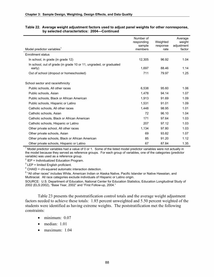
Chapter 3: Sample Design, Weighting, Design Effects, and Data Quality
Table 22. Average weight adjustment factors used to adjust panel weights for other nonresponse, by selected characteristics: 2004—Continued
Number of Average responding Weighted weight
Model predictor variables1 sample
members response
rate adjustment
factor Enrollment status
In school, in grade (in grade 12) 12,305 96.92 1.04 In school, out of grade (in grade 10 or 11, ungraded, or graduated
early) 1,697 88.46 1.14 Out of school (dropout or homeschooled) 711 79.97 1.25
School sector and race/ethnicity Public schools, All other races 6,538 95.60 1.06
Public schools, Asian 1,478 94.14 1.07 Public schools, Black or African American 1,913 91.69 1.09
Public schools, Hispanic or Latino 1,531 91.01 1.09 Catholic schools, All other races 1,448 98.95 1.01 Catholic schools, Asian 72 96.10 1.04
Catholic schools, Black or African American 171 97.64 1.03 Catholic schools, Hispanic or Latino 207 97.12 1.03
Other private school, All other races 1,134 97.80 1.03 Other private schools, Asian 69 93.82 1.07
Other private schools, Black or African American 85 91.20 1.12 Other private schools, Hispanic or Latino 67 87.84 1.35
1 Model predictor variables had a value of 0 or 1. Some of the listed model predictor variables were not actually in the model because they served as reference groups. For each group of variables, one of the categories (predictor variable) was used as a reference group. 2 IEP = Individualized Education Program. 3 LEP = limited English proficient. 4 CHAID = chi-squared automatic interaction detection. 5 “All other races” includes White, American Indian or Alaska Native, Pacific Islander or Native Hawaiian, and Multiracial. All race categories exclude individuals of Hispanic or Latino origin. SOURCE: U.S. Department of Education, National Center for Education Statistics, Education Longitudinal Study of 2002 (ELS:2002), “Base Year, 2002” and “First Follow-up, 2004.”
Table 23 presents the poststratification control totals and the average weight adjustment factors needed to achieve these totals: 1.85 percent unweighted and 5.50 percent weighted of the students were identified as having extreme weights. The poststratification met the following constraints:
• minimum: 0.07 • median: 1.01 • maximum: 1.04
88
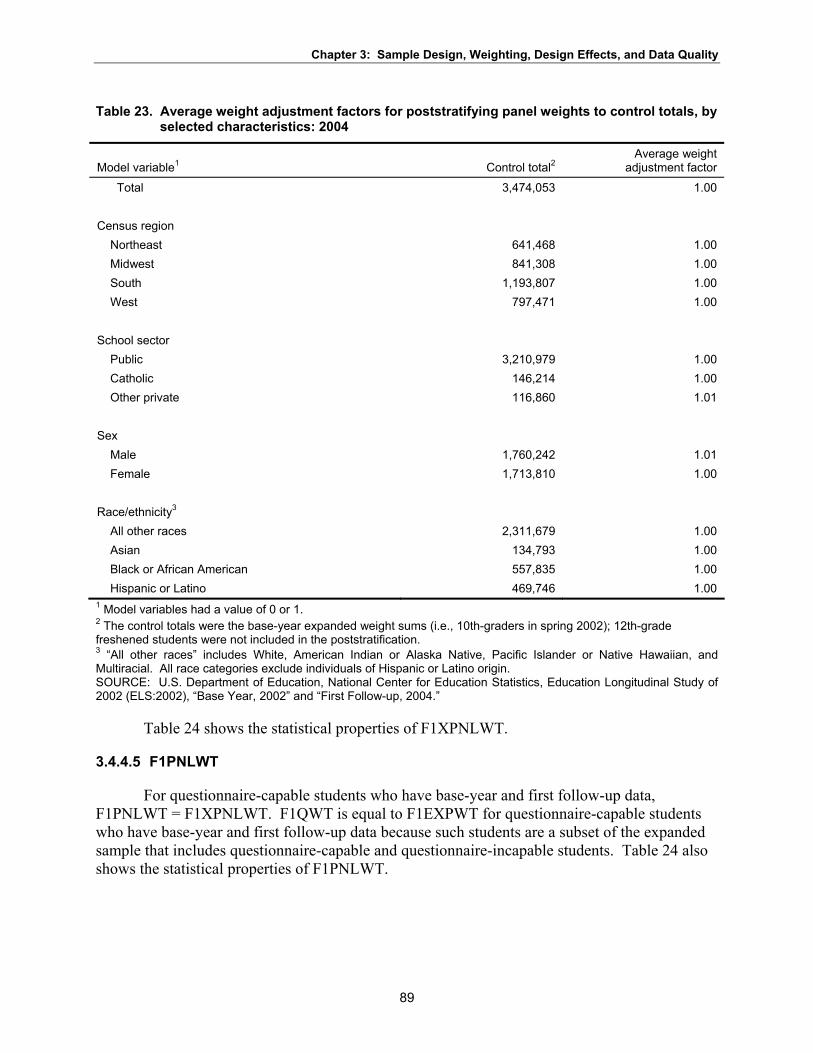
Chapter 3: Sample Design, Weighting, Design Effects, and Data Quality
Table 23. Average weight adjustment factors for poststratifying panel weights to control totals, by selected characteristics: 2004
Model variable1 Control total2 Average weight
adjustment factor Total 3,474,053 1.00
Census region Northeast 641,468 1.00 Midwest 841,308 1.00 South 1,193,807 1.00 West 797,471 1.00
School sector Public 3,210,979 1.00 Catholic 146,214 1.00 Other private 116,860 1.01
Sex Male 1,760,242 1.01 Female 1,713,810 1.00
Race/ethnicity3
All other races 2,311,679 1.00 Asian 134,793 1.00
Black or African American 557,835 1.00 Hispanic or Latino 469,746 1.00 1 Model variables had a value of 0 or 1. 2 The control totals were the base-year expanded weight sums (i.e., 10th-graders in spring 2002); 12th-grade freshened students were not included in the poststratification. 3 “All other races” includes White, American Indian or Alaska Native, Pacific Islander or Native Hawaiian, and Multiracial. All race categories exclude individuals of Hispanic or Latino origin. SOURCE: U.S. Department of Education, National Center for Education Statistics, Education Longitudinal Study of 2002 (ELS:2002), “Base Year, 2002” and “First Follow-up, 2004.”
Table 24 shows the statistical properties of F1XPNLWT.
3.4.4.5 F1PNLWT
For questionnaire-capable students who have base-year and first follow-up data, F1PNLWT = F1XPNLWT. F1QWT is equal to F1EXPWT for questionnaire-capable students who have base-year and first follow-up data because such students are a subset of the expanded sample that includes questionnaire-capable and questionnaire-incapable students. Table 24 also shows the statistical properties of F1PNLWT.
89

Chapter 3: Sample Design, Weighting, Design Effects, and Data Quality
Table 24. Statistical properties of panel weights: 2004
Weight F1PNLWT F1XPNLWT Mean 231.31 231.20 Variance 25,985.12 25,883.66 Standard deviation 161.20 160.88 Coefficient of variation (x 100) 69.69 69.59 Minimum 1.75 1.75 Maximum 1,445.49 1,445.49 Skewness 1.21 1.21 Kurtosis 2.48 2.49 Sum 3,403,321.11 3,441,475.79 Number of cases 14,713 14,885 SOURCE: U.S. Department of Education, National Center for Education Statistics, Education Longitudinal Study of 2002 (ELS:2002), “Base Year, 2002” and “First Follow-up, 2004.”
3.4.4.6 Quality Control
Quality control was emphasized on all activities, including weighting. Because of the central importance of the analysis weights to population estimation, a senior statistician thoroughly checked each set of weights. The most fundamental type of check was the verification of totals that are algebraically equivalent (e.g., marginal totals of the weights of eligible students prior to nonresponse adjustment and of respondents after nonresponse adjustment). In addition, various analytic properties of the initial weights, the weight adjustment factors, and the final weights were examined, both overall and within sampling strata, including
• distribution of the weights;
• ratio of the maximum weight divided by the minimum weight; and
• unequal weighting design effect, or variance inflation effect (1 + CV2).
Additionally, two-dimensional tables before and after weight adjustments were reviewed to ensure that the weight distribution was not distorted.
3.5 Standard Errors and Design Effects
3.5.1 Standard Errors For probability-based sample surveys, most estimates are nonlinear statistics. For
example, a mean or proportion, which is expressed as Σwy/Σw,25 is nonlinear because the denominator is a survey estimate of the (unknown) population total. In this situation, the variances of the estimates cannot be expressed in closed form. One common procedure for estimating variances of survey statistics is the Taylor series linearization procedure. This procedure takes the first-order Taylor series approximation of the nonlinear statistic and then substitutes the linear representation into the appropriate variance formula based on the sample design. Woodruff presented the mathematical formulation of this procedure (Woodruff 1971).
25 w is the estimated population, and y is a 0/1 variable indicating whether a certain characteristic is present for the sample member.
90

Chapter 3: Sample Design, Weighting, Design Effects, and Data Quality
The variance estimation must also take into account stratification and clustering. There are other variance estimation procedures, such as jackknife and balanced repeated replication (BRR). However, Taylor series estimation was used for the base year and is sufficient again for the first follow-up. Therefore, replicate weights were not produced. However, ELS:2002/04 will be available at a later date as a Data Analysis System (DAS). For the DAS, BRR replicate weights will be used.
Variance estimation procedures assumed a with-replacement design at the first stage of sampling. Because school sampling rates were moderately low, this assumption yields estimates that are only slightly biased in the positive direction. For stratified multistage surveys and a with-replacement sample design, the Taylor series procedure requires the specification of analysis strata and analysis primary sampling units (PSUs). In the base year, 361 analysis strata were formed from the sampling strata used in the first stage of sampling, and the analysis PSUs were the individual schools. Given that the school sample was selected using probability with minimum replacement (pmr), for variance estimation in the base year, variance estimation strata were formed consisting of two PSUs per stratum (Chromy 1981). However, when there was an odd number of schools in a sampling stratum, one of the analysis strata formed had three PSUs. The same analysis strata and PSUs as in the base year were used in the first follow-up. Each PSU still has at least two responding students. Students from new schools created by school splits (see section 3.3) are in the same strata and PSUs as they were for the base-year school. Also, freshened students are in the same strata and PSUs as the base-year students to whom they are linked.
As described in section 3.2, the ELS:2002 base-year sampling design was a stratified two-stage design. A stratified sample of schools was selected with probabilities proportional to a composite measure of size at the first stage, and a stratified systematic sample of students was selected from sample schools at the second stage. At the first stage, the school sampling rates varied considerably by school sampling strata. At the second stage, Asian and Hispanic students were sampled at higher rates than other students. Because of this complex sampling design, statistical analyses should be conducted using software that properly accounts for the complex survey design.
Many commonly used statistical computing packages assume that the data were obtained from a simple random sample; that is, they assume that the observations are independent and identically distributed. When the data have been collected using a complex sampling design, the simple random sampling assumption usually leads to an underestimate of the sampling variance, which would lead to artificially small confidence intervals and liberal hypothesis test results (i.e., rejecting the null hypothesis when it is in fact true more often than indicated by the nominal Type I error level) (Carlson, Johnson, and Cohen 1993).
Statistical strategies that have been developed to address this issue include first-order Taylor series expansion of the variance equation, balanced repeated replication, and the jackknife approach (Wolter 1985). Special-purpose software packages that have been developed for analysis of complex sample survey data include SUDAAN, WesVar, and Stata. Evaluations of the relative performances of these packages are reported by Cohen (1997).
91

Chapter 3: Sample Design, Weighting, Design Effects, and Data Quality
• SUDAAN is a commercial product developed by RTI; information regarding the features of this package and its lease terms is available from the website http://www.rti.org/sudaan.
• WesVar is a product of Westat, Inc.; information regarding the features of this package and its lease terms is available from the website http://www.westat.com/wesvar.
• Information regarding the features of Stata and its lease terms is available from the website http://www.stata.com.
• In addition to the variance estimation packages noted above, the American Institutes for Research (AIR) has developed the AM Statistical Software. AM software can be downloaded for free from the following website: http://am.air.org/.
Following is an example of generic SUDAAN code to produce estimates and standard errors using Taylor series. The symbols /* and */ in the code indicate the beginning and end of a comment. Note that the dataset must be sorted by analysis strata and analysis PSUs.
proc descript data=/* insert filename*/ design=wr;
nest analstr analpsu; /* these variables are the analysis strata and analysis PSUs,
respectively */
weight F1QWT;
var /*insert variables*/;
subpopn /* insert domain of interest if domain is a subset of students*/;
print nsum mean semean / style=nchs;
run;
3.5.2 Design Effects The impact of the departures of the ELS:2002 complex sample design from a simple
random sample design on the precision of sample estimates can be measured by the design effect. The design effect is the ratio of the actual variance of the statistic to the variance that would have been obtained had the sample been a simple random sample. The design standard errors will be different from the standard errors that are based on the assumption that the data are from a simple random sample. The ELS:2002 sample departs from the assumption of simple random sampling in three major respects: student samples were stratified by student characteristics, students were selected with unequal probabilities of selection, and the sample of students was clustered by school. A simple random sample is, by contrast, unclustered and not stratified. Additionally, in a simple random sample, all members of the population have the same probability of selection. Generally, clustering and unequal probabilities of selection
92

Chapter 3: Sample Design, Weighting, Design Effects, and Data Quality
increase the variance of sample estimates relative to a simple random sample, and stratification decreases the variance of estimates.
Standard errors and design effects were computed for all respondents and separately for only dropouts. Due to the lack of perfect overlap between questions on the student and dropout questionnaires and because dropouts were not administered tests, it was necessary to select two sets of 30 items. One set represents questions asked of all respondents, and the other set represents questions asked of all dropouts.
Standard errors and design effects were computed for 30 means and proportions overall for all respondents and dropouts and for subgroups of all respondents. They were not computed for subgroups of dropouts due to small cell sizes. The subgroups are similar to those used in NELS:88 and the ELS:2002 base year:
● sex (male and female); ● race/ethnicity (American Indian or Alaska Native, Asian or Pacific Islander, Black or
African American, Hispanic or Latino, More than one race, White and all other races);26
● school sector (public, Catholic, and other private); ● socioeconomic status (SES) (lowest quarter, middle two quarters, and highest
quarter); and ● urbanicity (urban, suburban, and rural).
Tables 3.3.1–9 and 3.3.1–15 from the NELS:88 second follow-up data file user’s manual (Ingels et al. 1994) were used to guide the items picked. For all respondents, it was often difficult to find an ELS:2002 item that matched exactly with the NELS:88 item. For dropouts, it was a little easier to find matching variables. The items chosen are a good representation of the different items on the ELS:2002 questionnaires. Therefore, these items should provide a range of data that give a reasonable average, as well as a reading on design effects for subgroups. However, because item matching with NELS:88 was difficult, the ELS:2002 design effects may not be comparable with the NELS:88 repeated design effects. Ideally, one would like to compare exact items between survey systems. Appendix K design effect tables from the ELS:2002 base-year data file user’s manual (Ingels et al. 2004) were not used to guide the items picked. Design effects were not expected to change much from the base year to the first follow-up, and it is more important to compare design effects across cohorts (e.g., ELS:2002 versus NELS:88) than to compare design effects from the base year with those from the first follow-up.
The student variables used were the versions after imputation, and all variables used were after disclosure avoidance (see sections 3.6 and 3.7). Also, the public versions of the variables were used when the public version differed from the restricted version. For all respondents and for dropouts, the standard errors and design effects were calculated using both the cross-sectional weight (F1QWT) and the panel weight (F1PNLWT). When using the panel weight, only panel respondents were included. The difference between the cross-sectional and panel respondents is
26 “White and all other races” is predominantly White, with a very small number of individuals from other race categories. All race categories exclude individuals of Hispanic or Latino origin.
93

Chapter 3: Sample Design, Weighting, Design Effects, and Data Quality
that base-year expanded sample students who responded in the first follow-up and freshened respondents are cross-sectional respondents but are not panel respondents. Expanded sample students were excluded from the analyses.
Appendix I contains tables of design effects for all respondents and dropouts. Each table includes the survey item (or composite variable), variable name and value, percent estimate, design standard error, simple random sample standard error, sample size (N), design effect (DEFF), and square root of the design effect (DEFT). Tables 25 and 26 summarize the average DEFFs and DEFTs for the full sample and panel sample, respectively, for all respondents, dropouts, and each subgroup. The reader should note that the mean DEFTs reported in tables 25, 26, and 27 were not calculated directly from the mean DEFF but, rather, are based on the summary statistics from the tables in appendix I.
Table 25. Mean design effects (DEFFs) and root design effects (DEFTs) for the first follow-up full sample, by selected characteristics: 2004
Characteristic Mean DEFF Mean DEFT
All respondents 2.26 1.47
Dropouts 1.31 1.14 Male 1.90 1.37 Female 1.94 1.37 American Indian or Alaska Native 1.51 1.22 Asian or Pacific Islander 2.14 1.44 Black or African American 1.49 1.21 Hispanic or Latino 1.59 1.25 More than one race 1.71 1.30 White and all other races1 1.84 1.35 Public schools 1.97 1.37 Catholic schools 2.25 1.46 Other private schools 3.02 1.66 Low socioeconomic status (SES) 1.66 1.27 Middle SES 1.68 1.29 High SES 1.91 1.38 Urban 2.85 1.64 Suburban 2.08 1.41 Rural 1.71 1.29
1 “White and all other races” is predominantly White, with a very small number of individuals from other race categories. All race categories exclude individuals of Hispanic or Latino origin. NOTE: The mean DEFT was not calculated directly from the mean DEFF but, rather, is the average DEFT over selected items. See appendix I of this document for more information. SOURCE: U.S. Department of Education, National Center for Education Statistics, Education Longitudinal Study of 2002 (ELS:2002), “First Follow-up, 2004.”
94

Chapter 3: Sample Design, Weighting, Design Effects, and Data Quality
Table 26. Mean design effects (DEFFs) and root design effects (DEFTs) for the first follow-up panel sample, by selected characteristics: 2004
Characteristic Mean DEFF Mean DEFT All respondents 2.23 1.46
Dropouts 1.31 1.14 Male 1.88 1.37 Female 1.93 1.37 American Indian or Alaska Native 1.50 1.21 Asian or Pacific Islander 2.17 1.44 Black or African American 1.49 1.22 Hispanic or Latino 1.60 1.25 More than one race 1.70 1.30 White and all other races1 1.83 1.35 Public schools 1.94 1.37 Catholic schools 2.25 1.46 Other private schools 3.00 1.65 Low socioeconomic status (SES) 1.64 1.26 Middle SES 1.67 1.29 High SES 1.92 1.38 Urban 2.80 1.63 Suburban 2.08 1.42 Rural 1.71 1.30
1 “White and all other races” is predominantly White, with a very small number of individuals from other race categories. All race categories exclude individuals of Hispanic or Latino origin. NOTE: The mean DEFT was not calculated directly from the mean DEFF but, rather, is the average DEFT over selected items. See appendix I of this document for more information. SOURCE: U.S. Department of Education, National Center for Education Statistics, Education Longitudinal Study of 2002 (ELS:2002), “First Follow-up, 2004.”
Table 27 shows the design effects from the BY for subgroups. The first follow-up design effects are lower for all respondents and for most of the subgroups than the base year design effects. For the full sample, the design effect for males is the same as in the base year, the design effects for American Indian or Alaska Native and for multiracial respondents are greater than in the base year, and the design effects for the other 14 subgroups are less than in the base year. For the panel sample, the design effects for American Indian or Alaska Native and for multiracial respondents are greater than in the base year, and the design effects for the other 15 subgroups are less than in the base year.
95

Chapter 3: Sample Design, Weighting, Design Effects, and Data Quality
Table 27. Mean design effects (DEFFs) and root design effects (DEFTs) for base-year student questionnaire data, by selected characteristics: 2002
Group Mean DEFF Mean DEFT All students 2.35 1.50
Male 1.90 1.37 Female 2.01 1.40 American Indian or Alaska Native 1.42 1.18 Asian or Pacific Islander 2.27 1.49 Black or African American 1.67 1.28 Hispanic or Latino 1.82 1.32 More than one race 1.63 1.27 White and all other races1 2.03 1.41 Public schools 2.07 1.41 Catholic schools 2.43 1.51 Other private schools 3.53 1.78 Low socioeconomic status (SES) 1.70 1.29 Middle SES 1.73 1.31 High SES 1.99 1.39 Urban 2.88 1.64 Suburban 2.15 1.44 Rural 1.94 1.37
1 “White and all other races” is predominantly White, with a very small number of individuals from other race categories. All race categories exclude individuals of Hispanic or Latino origin. NOTE: The mean DEFT was not calculated directly from the mean DEFF but, rather, is the average DEFT over selected items. See appendix I of this document for more information. SOURCE: U.S. Department of Education, National Center for Education Statistics, Education Longitudinal Study of 2002 (ELS:2002), “Base Year, 2002.”
The smaller design effects in the first follow-up compared with those in the base year may be due to the general tendency in longitudinal studies for design effects to lessen over time, as dispersion reduces the original clustering. In the first follow-up, as some of the sample members left the base-year school, the clusters of students within schools dispersed to an extent. Social characteristics of the sample members potentially varied to a greater extent as the clusters dispersed. Also, the weight trimming was more aggressive in the first follow-up than in the base year (i.e., the weights were trimmed for a larger percentage of the sample members in the first follow-up than in the base year). As discussed in section 3.4, trimming weights reduces the variance, which, by definition, reduces the design effect. Additionally, the items used to compute the mean design effects were different in the first follow-up than in the base year, because the design effects were not expected to change much between the two rounds of the study. It is more important to compare design effects across cohorts, as described below, so the items were chosen to be as comparable to NELS:88 second follow-up items as possible.
The design effects indicate that the ELS:2002 first follow-up full sample was more efficient than the NELS:88 second follow-up full sample and the HS&B first follow-up sophomore cohort full sample. For means and proportions based on first follow-up questionnaire
96

data for all respondents, the average design effect in ELS:2002 was 2.26; the comparable figures were 3.71 for the NELS:88 second follow-up and 3.59 for the HS&B sophomore cohort first follow-up. Figure 4 shows the mean design effects and root design effects for the HS&B first follow-up sophomore cohort, NELS:88 second follow-up, and ELS:2002 first follow-up. The difference in design effects is also apparent for some subgroup estimates. Ingels et al. (1994) present design effects for 16 subgroups defined similarly to those in table 25 above. For all 16 subgroups, the ELS:2002 design effects are smaller on average than those for the NELS:88 second follow-up.
Figure 4. Full sample mean design effects and root design effects, by longitudinal study: Selected years, 1972–2004
Value
3.6 3.7
2.3
1.8 1.9
1.5
0.0
0.5
1.0
1.5
2.0
2.5
3.0
3.5
4.0 Design effects Root design effects
HS&B first follow-up NELS:88 second ELS:2002 first sophomore cohort follow-up follow-up
Study
Chapter 3: Sample Design, Weighting, Design Effects, and Data Quality
SOURCE: U.S. Department of Education, National Center for Education Statistics, High School and Beyond (HS&B), “First Follow-up, 1980”; National Education Longitudinal Study of 1988 (NELS:88), “Second Follow-up, 1992”; and Education Longitudinal Study of 2002 (ELS:2002), “First Follow-up, 2004.”
The design effects indicate that the ELS:2002 panel sample (sophomore cohort) was more efficient than the NELS:88 F1F2 panel sample (sophomore cohort). For means and proportions based on first follow-up questionnaire data for all respondents, the average design effect in ELS:2002 was 2.23; the comparable figure was 3.73 for the NELS:88 sophomore cohort. Figure 5 shows the mean design effects and root design effects for the NELS:88 second follow-up and the ELS:2002 first follow-up sophomore cohort. The difference in design effects is also apparent for some subgroup estimates. Ingels et al. (1994) present design effects for 16 subgroups defined similarly to those in table 26 above. For all 16 subgroups, the ELS:2002 design effects are smaller on average than those for the NELS:88 sophomore cohort.
97

Figure 5. Mean design effects and root design effects, by NELS:88 and ELS:2002 panel sample (sophomore cohort): Selected years, 1988–2004
Value
4.0
3.5
3.0
2.5
2.0
1.5
1.0
0.5
0.0
3.7
2.3
1.9
1.5
NELS:88 second follow-up ELS:2002 first follow-up Study
Design effects Root design effects
Chapter 3: Sample Design, Weighting, Design Effects, and Data Quality
SOURCE: U.S. Department of Education, National Center for Education Statistics, National Education Longitudinal Study of 1988 (NELS:88), “Second Follow-up, 1992”; and Education Longitudinal Study of 2002 (ELS:2002), “First Follow-up, 2004.”
The design effects indicate that the ELS:2002 full and panel samples were also more efficient than the NELS:88 sample for dropouts. For means and proportions based on first follow-up questionnaire data for dropouts, the average design effect in ELS:2002 was 1.31 for both the full and panel samples; the comparable figures were 2.9 and 2.8 for the NELS:88 second follow-up full and F1F2 panel samples, respectively.
The smaller design effects in ELS:2002 compared with those for NELS:88 and HS&B are probably due to subsampling. Nonrespondents were subsampled in the ELS:2002 first follow-up, but additional subsampling was done in the other studies. In NELS:88, no subsampling was done in the second follow-up, but several types of sample members, including nonrespondents, were subsampled. Additionally, disproportional strata representation was introduced by subsampling in the NELS:88 first follow-up. Dropouts were retained with certainty, whereas other students were subsampled at different rates. See Ingels et al. (1994) for more details. In HS&B, the sophomore cohort members who were no longer in the base-year school were subsampled. See Spencer et al. (1987) for more details. As mentioned above, the general tendency in longitudinal studies is for design effects to lessen over time, as dispersion reduces the original clustering. Subsampling increases design effects because it introduces additional variability into the weights with an attendant loss in sample efficiency.
The smaller design effects in ELS:2002 compared with those for the HS&B sophomore cohort also may reflect the somewhat smaller cluster size used in the later survey in the base year. Although the clusters were reduced somewhat in the first follow-up for both studies, a number of students remained in the base-year school. The HS&B base-year sample design
98

DEFFc = 1 + (b – 1) rho,
Chapter 3: Sample Design, Weighting, Design Effects, and Data Quality
called for 36 sophomores selected from each school. The ELS:2002 sample design called for about 26 sophomores selected from each school. Clustering tends to increase the variance of survey estimates because the observations within a cluster are similar and therefore add less information than independently selected observations. The impact of clustering depends mainly on two factors: the number of observations within each cluster and the degree of within-cluster homogeneity. When cluster sizes vary, the impact of clustering (DEFFc) can be estimated by
DEFFc = 1 + (b – 1) rho,
where b refers to the average cluster size (the average number of students selected from each school) and rho refers to the intraclass correlation coefficient, a measure of the degree of within-cluster homogeneity. If the value of rho (which varies from one variable to the next) averaged about 0.05 in both studies, then the reduced cluster size in ELS:2002 would almost exactly account for the reduction in the design effects relative to HS&B.
If one must perform a quick analysis of ELS:2002 data without using one of the software packages for analysis of complex survey data, the design effects tables in appendix I can be used to make approximate adjustments to the standard errors of survey statistics computed using the standard software packages that assume simple random sampling designs. One cannot be confident regarding the actual design-based standard error without performing the analysis using one of the software packages specifically designed for analysis of data from complex sample surveys.
Standard errors for a proportion can be estimated from the standard error computed using the formula for the standard error of a proportion based on a simple random sample and the appropriate DEFT:
SE = DEFT * (p(1-p)/n)1/2.
Similarly, the standard error of a mean can be estimated from the weighted variance of the individual scores and the appropriate mean DEFT:
SE = DEFT * (Var/n)1/2.
Tables 25, 26, and 27 make it clear that the DEFFs and DEFTs vary considerably by subgroup. It is therefore important to use the mean DEFT for the relevant subgroup in calculating approximate standard errors for subgroup statistics.
Standard error estimates may be needed for subgroups that are not shown in the appendix. One rule of thumb may be useful in such situations. The general rule states that design effects will generally be smaller for groups that are formed by subdividing the subgroups listed in the tables. (Smaller subgroups will be affected less by clustering than larger subgroups; in terms of the equation for DEFFc, b will be reduced.) Estimates for Hispanic males, for example, will generally have smaller design effects than the corresponding estimates for all Hispanics or all males. For this reason, it will usually be conservative to use the subgroup mean DEFT to approximate standard errors for estimates concerning a portion of the subgroup. This rule only applies when the variable used to subdivide a subgroup crosscuts schools. Sex is one
99

Chapter 3: Sample Design, Weighting, Design Effects, and Data Quality
such variable because most schools include students of both sexes. It will not reduce the average cluster size to form groups that are based on subsets of schools.
Standard errors may also be needed for other types of estimates than the simple means and proportions that are the basis for the results presented in the above tables. A second method can be used to estimate approximate standard errors for comparisons between subgroups. If the subgroups crosscut schools, then the design effect for the difference between the subgroup means will be somewhat smaller than the design effect for the individual means; consequently, the variance of the difference estimate will be less than the sum of the variances of the two subgroup means from which it is derived:
Var(b-a) = Var(b) + Var(a)
where Var(b-a) refers to the variance of the estimated difference between the subgroup means, and Var(a) and Var(b) refer to the variances of the two subgroup means. This equation assumes that the covariance of the subgroup means is negligible. It follows from this equation that Var(a) + Var(b) can be used in place of Var(b-a) with conservative results.
A final principle is that more complex estimators show smaller design effects than simple estimators (Kish and Frankel 1974). Thus, correlation and regression coefficients tend to have smaller design effects than subgroup comparisons, and subgroup comparisons have smaller design effects than means. This principle implies that it will be conservative to use the DEFTs in the above tables in calculating approximate standard errors for complex statistics, such as multiple regression coefficients. The procedure for calculating such approximate standard errors is the same as with simpler estimates: first, a standard error is calculated using the formula for data from a simple random sample; then the standard error is multiplied by the appropriate DEFT.
One analytic strategy for accommodating complex survey designs is to use the mean design effect to adjust for the effective sample size resulting from the design. For example, one could create a weight that is the multiplicative inverse of the design effect and use that weight (in conjunction with sampling weights) to deflate the obtained sample size to take into account the inefficiencies due to a sample design that is a departure from a simple random sample. Using this procedure, statistics calculated by a statistical program such as SAS or SPSS will reflect the reduction in sample size in the calculation of standard errors and degrees of freedom. Such techniques capture the effect of the sample design on sample statistics only approximately. However, while not providing a full accounting of the sample design, this procedure provides some adjustment for the sample design and is probably better than conducting analysis that assumes the data were collected from a simple random sample. The analyst applying this correction procedure should carefully examine the statistical software being used and assess whether or not the program treats weights in such a way as to produce the effect described above.
100

Chapter 3: Sample Design, Weighting, Design Effects, and Data Quality
3.6 Imputation
3.6.1 Imputation Variables Eighteen key analysis variables were selected for imputation for the ELS:2002 first
follow-up study. These variables included the same variables that were chosen for imputation in the base-year study and two new variables from the first follow-up study. Table 28 lists the selected variables. The two new variables selected for imputation include the spring 2004 student ability estimate for mathematics and the spring 2004 student enrollment status (e.g., in school in grade 12, in school in other grade or ungraded or early graduate, out of school because of dropout or homeschooled, or out of scope/ineligible). These variables were chosen because they are standard classification variables used in most data reporting.
Table 28. First follow-up imputation variables, by number and weighted proportion imputed: 2004
Weighted percent Number of cases Variable imputed imputed1
Student sex 1 0.01 Student race/ethnicity 6 0.04 Student language minority status 33 0.20 Student Hispanic subgroup2 14 0.09 Student Asian subgroup2 12 0.07 School program type 651 4.01 Student postsecondary educational expectations 91 0.56 Parental aspirations for student postsecondary achievement 687 4.23 Family composition 65 0.40 Mother’s educational attainment3 111 0.68 Mother’s occupation3 166 1.02 Father’s educational attainment3 183 1.13 Father’s occupation3 237 1.46 Family income (2001)3 868 5.34 Enrollment status (in school vs. out) 86 0.53 Spring 2004 student ability estimate (theta) for mathematics4 2,707 16.66 10th-grade student ability estimate (theta) for mathematics4 651 4.01 10th-grade student ability estimate (theta) for reading4 651 4.01 1 The denominator used in calculating the weighted percent missing varies by variable due to restrictions on eligibility for imputation. 2 All race categories exclude individuals of Hispanic or Latino origin. 3 Used to construct socioeconomic status (SES). 4 Used to construct scale, quartile, and proficiency scores. SOURCE: U.S. Department of Education, National Center for Education Statistics, Education Longitudinal Study of 2002 (ELS:2002), “First Follow-up, 2004.”
3.6.2 Imputation Methodologies The ELS:2002 base-year and first follow-up data files were imputed using three
imputation methods including logical imputation, weighted sequential hot deck imputation, and
101

Chapter 3: Sample Design, Weighting, Design Effects, and Data Quality
multiple imputation. This section gives a brief summary of each of these methods and outlines how each one was used in the imputation plan.
All possible logical imputations were performed before any other imputation method was applied to the data files. For instance, student sex was imputed by assigning a value based on student name. This assignment mapping was developed using the distribution of the known student names and sex values. Student sex and student race were the only two variables that were logically imputed.
After all logical imputations were completed, weighted sequential hot deck imputation (Cox 1980) was used to impute 13 categorical variables. Sequential hot deck imputation is a common procedure used for item nonresponse. This method uses the respondent survey data (donors) to provide imputed values for records with missing values. The basic principle of sequential hot deck imputation involves defining imputation classes, which generally consist of a cross-classification of covariates, and then replacing missing values sequentially from a single pass through the survey data within the imputation classes. When sequential hot deck imputation is performed using the sampling weights of the item respondents and nonrespondents, the procedure is called weighted sequential hot deck imputation. This procedure takes into account the unequal probabilities of selection in the original sample by using the sampling weight to specify the expected number of times a particular respondent’s answer was used to replace a missing item. These expected selection frequencies are specified so that, over repeated applications of the algorithm, the expected value of the weighted distribution of the imputed values will equal in expectation within imputation class the weighted distribution of the reported answers. Weighted sequential hot deck imputation was chosen for most of the variables because this procedure works well for categorical data.
The last imputation procedure used was multiple imputation (MI). The MI procedure was chosen for three continuous variables: the 10th-grade student ability estimate (theta) for mathematics, the 10th-grade student ability estimate (theta) for reading, and the spring 2004 student ability estimate (theta) for mathematics. MI is a technique that requires imputing missing values several times and creating m complete datasets. These are created such that regular complete-case analyses can be performed. The parameters of interest, then, can be calculated by averaging the parameter estimators from each augmented dataset. The SAS PROC MI procedure was used to impute these three variables. The Markov Chain Monte Carlo (MCMC) model option, which assumes the data are from a multivariate normal distribution, was used to estimate the entire joint posterior probability distribution of the unknown quantities. Random draws from this distribution were taken to fill in the missing values.
The SAS PROC MI procedure was selected for these three variables because it provides an imputation variance based on MI theory and does not require any additional computation. The “theta” value (which is only a restricted-use variable) is used in the construction of various ELS:2002 test variables, and this construction process requires an imputation variance.
It should be noted that MI was not chosen for imputation of all variables, because the MI procedure is currently restricted to imputation of continuous variables and most of the variables selected for imputation are categorical. Therefore, the weighted sequential hot deck was the preferred method for these variables.
102

Chapter 3: Sample Design, Weighting, Design Effects, and Data Quality
3.6.3 Definition of Eligibility for Imputation Table C-1 in appendix C shows the set of respondents for which each variable was
imputed. The appendix lists the different respondent types, including the questionnaire-ineligible (expanded sample) students. As shown in the appendix, all variables were imputed for base-year nonrespondents who became first follow-up respondents (651 students) and for base-year respondents who were also first follow-up respondents (14,062). For base-year questionnaire-incapable students whose status had changed 2 years later and who were successfully surveyed in the first follow-up (n = 105), all variables were imputed except school program type and the 10th-grade ability estimates. For freshened respondents (171), all variables were imputed except school program type, the 10th-grade ability estimates, and parental aspirations. For the first follow-up questionnaire-incapable students (100), all variables were imputed except school program type, student postsecondary educational expectations, and the student ability estimates.
The 16 variables that were imputed in the base-year study were not imputed again for base-year nonrespondents because their data were either reported or imputed in the base year. These variables were only imputed in the first follow-up when not provided by respondents in the new participant supplement by first follow-up respondents who were base-year nonrespondents, 12th-grade freshened sample members, or base-year questionnaire-ineligible students who became first follow-up respondents. The base-year nonrespondents who became first follow-up respondents included students still at the base-year school, transfer students, dropouts, early graduates, and homeschooled students.
The spring 2004 student ability estimate for mathematics was imputed for students who were considered in school (i.e., students still attending the sample school as of spring 2004 and transfer students as of spring 2004). The estimate was not imputed for out-of-school respondents (i.e., dropouts, early graduates, and homeschooled students). For the 651 students who became first follow-up respondents and were base-year nonrespondents, the 10th-grade student ability estimates for mathematics and reading were imputed.
Finally, spring 2004 enrollment status for all first follow-up sample members (respondents and nonrespondents) on the restricted-use file (16,374) was imputed. Most information was imputed using data available from school records, and any remaining missing data were imputed using the weighted sequential hot deck procedure. This variable was imputed because it is an analysis variable that will be used frequently, and it provides a better picture of the cohort dropout rate.
3.6.4 Imputation Results Of the 15 categorical variables, 2 variables (sex and race/ethnicity) were imputed using
logical imputation, and 13 were imputed using a weighted sequential hot deck procedure. The remaining 3 continuous variables were imputed using MI.
Table 28 lists the variables in the order in which they were imputed and shows the number of cases that were imputed. The order in which the variables were imputed depended on whether the response of one variable was dependent upon the response of another variable. For instance, Hispanic and Asian subgroup could only be imputed after the race/ethnicity variable
103

Chapter 3: Sample Design, Weighting, Design Effects, and Data Quality
was determined. Similarly, family income was dependent on parent education and occupation; therefore, parent education and occupation were imputed prior to family income. Within these dependencies, the variables were imputed in the same order that they were imputed in the base-year study, generally starting with the variable containing the lowest percentage missing up to the variable with the highest percentage missing.
The basic MI model used for imputing the student ability estimates included the following predictor variables: sex, race/ethnicity, student language, student postsecondary aspirations, parental aspirations for student, family composition, mother’s and father’s occupation and education level, household income, school type, urbanicity, and census region. The model used for predicting the spring 2004 student ability estimate in mathematics also contained the 10th-grade ability estimate for both mathematics and reading. Similarly, the model used for predicting the 10th-grade ability estimate for both mathematics and reading contained the spring 2004 student ability estimate in mathematics.
Table C-2 presents the imputation classes and sorting variables used for all of the variables imputed by the weighted sequential hot deck approach, and table C-3 presents the variables used in the MI models. Table C-4 presents the before- and after-imputation distributions.
3.6.5 Imputation Evaluation The key measure for determining whether the imputation methods produce acceptable
results is that the before- and after-imputation weighted distributions are similar. For evaluation of the imputation results, distributions were considered to be similar when absolute differences are less than 5 percent where the absolute difference is calculated by subtracting the before- imputation weighted percent from the after-imputation weighted percent. If absolute differences are greater than 5 percent, then the unweighted distributions were examined to see if the large differences are due to small sample sizes. Any large differences were evaluated and corrected when possible (perhaps by using different imputation classes) and documented when no resolution is possible.
MI inference assumes that the analyst’s model is the same as the imputer’s model. However, the two models may not be the same. Therefore, a general practice is to include as many variables as possible when doing MI. The precision that is lost when unimportant predictors are included is usually relatively small compared with the general validity of analyses of the resultant multiply imputed dataset. The PROC MI procedure provides the between- imputation, within-imputation, and total variances for the model. Additionally, it provides the degrees of freedom for the total variance, the relative increase in variance due to missing values, and the fraction of missing information for each parameter estimate. These statistics were used in the evaluation of the MI.
3.7 Disclosure Risk Analysis and Protections Because of the paramount importance of protecting the confidentiality of NCES data that
contain information about specific individuals, ELS:2002 first follow-up data were subject to various procedures to minimize disclosure risk.
104
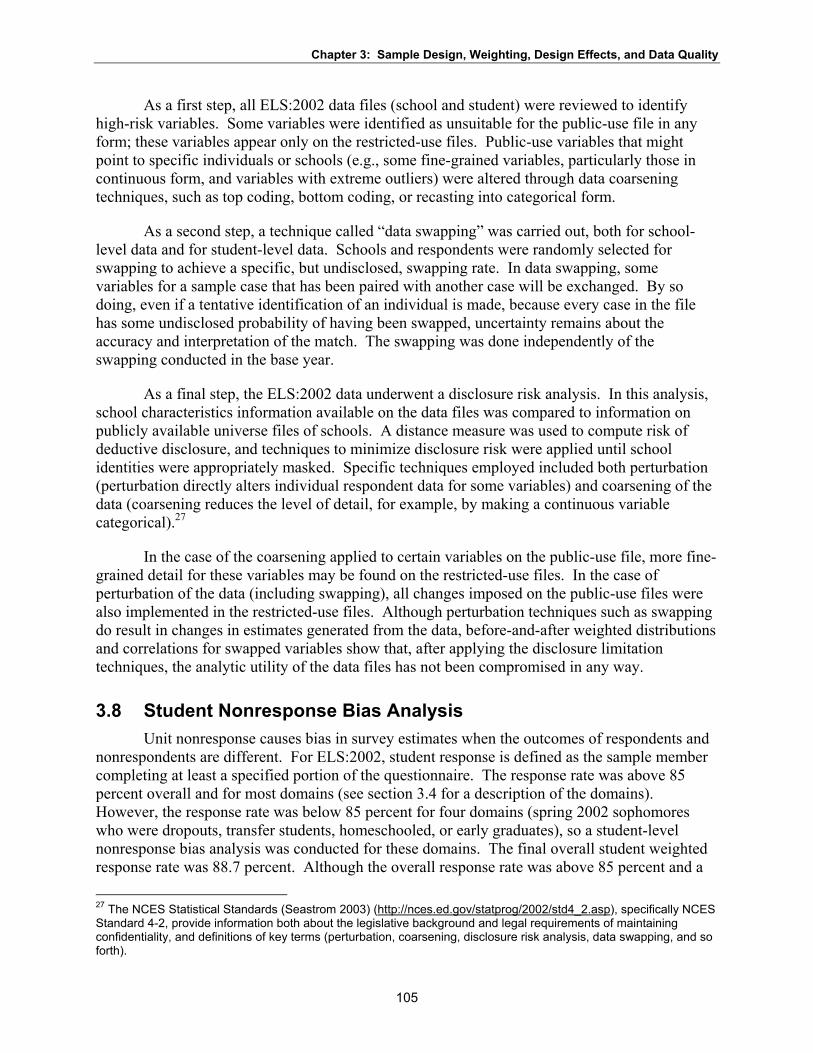
Chapter 3: Sample Design, Weighting, Design Effects, and Data Quality
As a first step, all ELS:2002 data files (school and student) were reviewed to identify high-risk variables. Some variables were identified as unsuitable for the public-use file in any form; these variables appear only on the restricted-use files. Public-use variables that might point to specific individuals or schools (e.g., some fine-grained variables, particularly those in continuous form, and variables with extreme outliers) were altered through data coarsening techniques, such as top coding, bottom coding, or recasting into categorical form.
As a second step, a technique called “data swapping” was carried out, both for school-level data and for student-level data. Schools and respondents were randomly selected for swapping to achieve a specific, but undisclosed, swapping rate. In data swapping, some variables for a sample case that has been paired with another case will be exchanged. By so doing, even if a tentative identification of an individual is made, because every case in the file has some undisclosed probability of having been swapped, uncertainty remains about the accuracy and interpretation of the match. The swapping was done independently of the swapping conducted in the base year.
As a final step, the ELS:2002 data underwent a disclosure risk analysis. In this analysis, school characteristics information available on the data files was compared to information on publicly available universe files of schools. A distance measure was used to compute risk of deductive disclosure, and techniques to minimize disclosure risk were applied until school identities were appropriately masked. Specific techniques employed included both perturbation (perturbation directly alters individual respondent data for some variables) and coarsening of the data (coarsening reduces the level of detail, for example, by making a continuous variable categorical).27
In the case of the coarsening applied to certain variables on the public-use file, more fine-grained detail for these variables may be found on the restricted-use files. In the case of perturbation of the data (including swapping), all changes imposed on the public-use files were also implemented in the restricted-use files. Although perturbation techniques such as swapping do result in changes in estimates generated from the data, before-and-after weighted distributions and correlations for swapped variables show that, after applying the disclosure limitation techniques, the analytic utility of the data files has not been compromised in any way.
3.8 Student Nonresponse Bias Analysis Unit nonresponse causes bias in survey estimates when the outcomes of respondents and
nonrespondents are different. For ELS:2002, student response is defined as the sample member completing at least a specified portion of the questionnaire. The response rate was above 85 percent overall and for most domains (see section 3.4 for a description of the domains). However, the response rate was below 85 percent for four domains (spring 2002 sophomores who were dropouts, transfer students, homeschooled, or early graduates), so a student-level nonresponse bias analysis was conducted for these domains. The final overall student weighted response rate was 88.7 percent. Although the overall response rate was above 85 percent and a
27 The NCES Statistical Standards (Seastrom 2003) (http://nces.ed.gov/statprog/2002/std4_2.asp), specifically NCES Standard 4-2, provide information both about the legislative background and legal requirements of maintaining confidentiality, and definitions of key terms (perturbation, coarsening, disclosure risk analysis, data swapping, and so forth).
105

Chapter 3: Sample Design, Weighting, Design Effects, and Data Quality
nonresponse bias analysis is not required by NCES standards, a bias analysis for base-year sophomores was conducted for the purposes of quality and completeness using both the cross-sectional and panel weights.
The nonresponse bias was estimated for variables known for both respondents and nonrespondents. In the base year, information was not collected for nonresponding students other than what was received on the student enrollment lists. On these lists, data were obtained on IEP status, race/ethnicity, and sex. These data were not provided by all schools (in particular, information on IEP status was often missing, and IEP information was typically relevant only for public schools). In consequence, only the school-supplied race/ethnicity and sex data were used. For most of the first follow-up freshened students, race/ethnicity and sex data were available. The student’s spring 2004 enrollment status was also used and defined as follows:
• in school, in grade (in grade 12);
• in school, out of grade (in grade 10 or 11, ungraded, or graduated early); and
• out of school (dropout or homeschooled).
There were also extensive data available for schools from the base-year school administrator questionnaire, so these data were used to help reduce potential nonresponse bias. Students were linked to the base-year school from which they were sampled. The first follow-up administrator data were not used when available because it is possible that student nonresponse is correlated with school nonresponse. It was safer to use the base-year administrator data for all students. The school sampling frame constructed from the CCD and PSS also contains data for all base-year schools. School data used included the following:
• school sector;
• urbanicity;
• region;
• sophomore enrollment;
• total enrollment;
• number of minutes per class;
• number of class periods;
• number of school days;
• number of students receiving free or reduced-price lunch;
• number of full-time teachers;
• percentage of full-time teachers certified;
• number of part-time teachers;
• number of different grades taught at the school;
• school level;
• coeducational status;
106

Chapter 3: Sample Design, Weighting, Design Effects, and Data Quality
• percentage of students with an IEP;
• percentage of students with LEP;
• percentage Hispanic or Latino sophomores;
• percentage Asian sophomores;
• percentage Black or African American sophomores; and
• percentage All other race sophomores (includes White).
The procedures used for the nonresponse bias analysis were similar to those used in the base year. First, for the school and student data known for most respondents and nonrespondents, the nonresponse bias was estimated and tested to determine if the bias was significant at the 5 percent level. Second, nonresponse adjustments were computed, and variables known for most respondents and nonrespondents were included in the nonresponse models. The nonresponse adjustments described in section 3.4 were designed to significantly reduce or eliminate nonresponse bias for variables included in the models. Variables not known for most respondents and nonrespondents could not be included in the nonresponse adjustments, and therefore nonresponse bias could not explicitly be reduced for these variables. However, many of the variables in the nonresponse models are correlated with many of the other variables.
Third, after the school and student weights were computed, remaining bias for data known for most respondents and nonrespondents was estimated and statistically tested to check if there was any remaining significant nonresponse bias. Fourth, the remaining bias after student weight adjustments was divided by the standard error, that is, bias/standard error.
The bias in an estimated mean based on respondents, yR , is the difference between this mean and the target parameter, B (i.e., the mean that would be estimated if a complete census of the target population was conducted). This bias can be expressed as follows:
B y( ) = yr −πR
The estimated mean based on nonrespondents, yNR , can be computed if data for the particular variable for most of the nonrespondents are available. The estimation of π is as follows:
ˆ (1 η ) yR +η y Rπ = − N
where η is the weighted unit nonresponse rate. For the variables that are from the frame rather than from the sample, B can be estimated without sampling error. Therefore, the bias can be estimated as follows:
B yR = y −π̂ˆ ( ) R
or equivalently
107

Chapter 3: Sample Design, Weighting, Design Effects, and Data Quality
B̂ ( y ) =η ( y − y )R R NR
This formula shows that the estimate of the nonresponse bias is the difference between the mean for respondents and nonrespondents multiplied by the weighted nonresponse rate. The variance of the bias was computed using Taylor series estimation in RTI’s software package SUDAAN.
Tables 29 and 30 show the nonresponse bias before and after weight adjustments for selected variables for base-year sophomores. The first set of columns in each table shows the estimated bias before nonresponse adjustment for the variables available for most responding and nonresponding students. The results are identical for these two tables. Statistical tests (t tests) were used to test each level of the variables for significance of the bias at the 0.05/(c-1) significance level, where c is the number of categories (levels) within the primary variable. Below is a summary of the before-adjustment significant bias for tables 29 and 30:
• At least one level of 9 of the 25 variables was biased in each table.
• Sixteen levels of variables were found to be significantly biased in both tables 29 and 30.
• Significant biases were usually small.
The second set of columns in tables 29 and 30 shows the estimated bias after weight adjustments (using F1QWT for table 29 and F1PNLWT for table 30) for the variables available for most responding and nonresponding students. The bias after weight adjustments was computed as the difference between the estimate using nonresponse-adjusted (final) weights and the estimate using the design (base) weights prior to nonresponse adjustment. This latter estimate is an estimate of B because it is the estimate of the target population using the design weights. Similar to the testing of before-adjustment bias, t tests were performed to test the significance of the bias for each level of the variables. In both tables 29 and 30, the estimated bias usually decreased after weight adjustments. Therefore, the number of significantly biased levels of variables decreased from 16 before adjustment to zero after adjustment in both tables.
Tables 31, 32, 33, and 34 show the nonresponse bias before and after weight adjustments for selected variables in domains where the response rate was less than 85 percent. Table 31 refers to the domain of transfer students, table 32 refers to the domain of dropouts, table 33 refers to the domain of early graduates, and table 34 refers to the domain of homeschooled students. As in tables 29 and 30, the first set of columns in each table shows the estimated bias before nonresponse adjustment for the variables available for most responding and nonresponding students. Statistical tests (t tests) were again used to test the significance of the bias at the 0.05/(c-1) significance level. Below is a summary of the before-adjustment significant bias for tables 31, 32, 33, and 34:
• At least one level of three variables and a total of four levels were found to be significantly biased in table 31.
• One level of two variables was found to be significantly biased in table 32.
• One level of five variables was found to be significantly biased in table 33.
108

Chapter 3: Sample Design, Weighting, Design Effects, and Data Quality
• At least one level of four variables and a total of five levels were found to be significantly biased in table 34.
• Significant biases were usually small.
As in tables 29 and 30, the second set of columns in tables 31, 32, 33, and 34 shows the estimated bias after weight adjustments (using F1QWT) for the variables available for most responding and nonresponding students. The bias after weight adjustments was computed the same way as described above for tables 29 and 30. Statistical tests (t tests) were performed to test the significance of the bias for each level of the variables. In all four tables, the estimated bias sometimes decreased after weight adjustments and sometimes increased after weight adjustments. In tables 31 and 32, the amount of significant bias actually increased to seven levels of four variables and five levels of three variables, respectively. In tables 33 and 34, the amount of significant bias decreased to one and zero variables, respectively. Note that sample members are assigned to these domains based on data known for respondents and nonrespondents, and sample members may actually be in different domains. Therefore, these bias estimates are approximate. Also, the weight adjustments accounted for enrollment status, as described in section 3.4, but enrollment status combined the categories of transfer student, dropout, early graduate, or homeschooled student. Enrollment status was used because it was considered the more important analysis variable and to be consistent with NELS:88.
The student nonresponse bias analyses in conjunction with the weighting adjustments described below do not eliminate all bias. They reduce bias for some of the variables known for most respondents and nonrespondents, which are considered to be some of the analytically important variables and are correlated with many of the other variables. Significant bias after weight adjustments is minimal for the variables analyzed. Some of these variables are used to help create composite (or derived) variables. There may be bias remaining in other variables.
Figures 6 through 11 compare the estimated relative bias before nonresponse adjustment with the estimated relative bias after nonresponse adjustment for base-year sophomores using F1QWT, base-year sophomores using F1PNLWT, transfer students using F1QWT, dropouts using F1QWT, early graduates using F1QWT, and homeschooled students using F1QWT, respectively. Relative bias is the bias of the estimate divided by the estimate. It provides an indication of the order of magnitude of the bias with respect to the estimate. Figures 6 and 7 indicate that when the relative bias was large before nonresponse adjustment, it was almost always reduced after nonresponse adjustment. When the relative bias was small before nonresponse adjustment, it stayed small after nonresponse adjustment with occasional small increases. These two figures clearly show that the nonresponse adjustment reduced bias for base-year sophomores. Figures 8 through 11 show somewhat of a random pattern. Sometimes relative bias decreased after nonresponse adjustment, sometimes relative bias increased after nonresponse adjustment, and sometimes, relative bias did not change much after nonresponse adjustment. As shown in tables 32 through 34, the bias is frequently not significant after nonresponse adjustment. Also, as mentioned above, sample members are assigned to these domains based on data known for respondents and nonrespondents, and sample members may actually be in different domains.
109

Chapter 3: Sample Design, Weighting, Design Effects, and Data Quality
Nonresponse bias can have an effect on significance testing. Tables 29 through 34 include an estimate of the bias ratio (student bias divided by the standard error). If this ratio is larger than 2 percent, then the probability of a Type I error is greater than 0.05. Figures 12 through 17 show the student bias ratio by the Type I error rate for base-year sophomores using F1QWT, base-year sophomores using F1PNLWT, transfer students, dropouts, early graduates, and homeschooled students, respectively. Figures 12 and 13 show that for many of the student variables included in the nonresponse bias analysis, the Type I error rate is at or close to 0.05, and outliers were not graphed. These results are similar to the base-year results for spring 2002 sophomores. Figures 14 through 17 show that although some variables have a Type I error rate at or near 0.05, there are more variables that have a higher Type I error rate. These figures do not take the school bias ratio into account. The school bias ratio varies by school variable, as shown in the ELS:2002 base-year data file user’s manual (Ingels et al. 2004). If it is assumed that the school bias ratio is zero, then there is no effect on the student bias ratio. However, if the school bias ratio is large, then the Type I error rates are larger. Although the tables above show that nonresponse bias is minimal, the data user should exercise caution when conducting statistical tests.
110

Table 29. Nonresponse bias before and after nonresponse adjustment for base-year sophomores using the cross-sectional weight, by selected categorical variables: 2004
Before nonresponse adjustment After nonresponse adjustment Overall Overall
Non- mean, mean,
Description Unweighted respondents
Unweighted non-
respondents
Respondent mean
weighted1
respondent mean
weighted1
Esti-mated
bias Relative
bias SIG2
before adjust-ments1
after adjust-ments3
Esti-mated
bias
Bias per standard
error Relative
bias SIG2
Asian 10th-grade enrollment percent ≤ 2 percent 5,684 547 38.298 39.784 -0.167 -0.004 N 38.465 38.686 -0.221 -0.461 -0.006 N > 2 percent 9,029 943 61.702 60.216 0.167 0.003 N 61.535 61.314 0.221 0.461 0.004 N
Black or African American 10th-grade enrollment percent
≤ 4 percent 5,043 459 34.669 32.029 0.296 0.009 N 34.373 34.296 0.076 0.150 0.002 N > 4 percent 9,670 1031 65.331 67.971 -0.296 -0.005 N 65.627 65.704 -0.076 -0.150 -0.001 N
Minutes per class period ≤ 45 3,540 368 18.887 21.081 -0.246 -0.013 N 19.133 19.144 -0.011 -0.031 -0.001 N
46–50 3,166 312 21.924 20.110 0.203 0.009 N 21.720 21.662 0.059 0.110 0.003 N 51–80 3,925 394 28.983 29.746 -0.086 -0.003 N 29.068 29.036 0.033 0.066 0.001 N 81+ 4,082 416 30.206 29.063 0.128 0.004 N 30.078 30.159 -0.081 -0.180 -0.003 N
Class periods per day 1–4 4,219 421 31.191 28.889 0.258 0.008 N 30.933 31.021 -0.088 -0.195 -0.003 N 5–6 3,612 403 26.901 29.533 -0.295 -0.011 N 27.196 27.129 0.067 0.144 0.002 N
7 3,984 400 24.649 25.304 -0.073 -0.003 N 24.722 24.742 -0.019 -0.047 -0.001 N 8–9 2,898 266 17.259 16.274 0.111 0.006 N 17.149 17.109 0.040 0.087 0.002 N
Is the school coeducational? Yes 13,937 1,425 97.909 98.506 -0.067 -0.001 N 97.976 97.970 0.006 0.150 # N
No, all-female school 361 35 1.004 0.890 0.013 0.013 N 0.992 0.991 # 0.014 # N No, all-male school 415 30 1.087 0.604 0.054 0.052 N 1.032 1.039 -0.007 -0.283 -0.007 N
Student race/ethnicity4
All other races 9,120 830 67.450 62.158 0.594 0.009 Y 66.857 66.818 0.039 0.089 0.001 N Asian 1,619 173 3.891 3.623 0.030 0.008 N 3.861 3.853 0.008 0.071 0.002 N
Black or African American 2,169 261 15.708 18.383 -0.300 -0.019 N 16.008 15.985 0.022 0.075 0.001 N Hispanic or Latino 1,805 226 12.951 15.836 -0.324 -0.024 N 13.275 13.344 -0.069 -0.247 -0.005 N
10th-grade enrollment 0–99 2,888 255 12.689 9.164 0.395 0.032 Y 12.294 12.337 -0.043 -0.092 -0.004 N 100–249 3,823 293 22.457 16.644 0.652 0.030 Y 21.805 21.947 -0.142 -0.412 -0.007 N 250–499 4,704 485 36.049 38.916 -0.322 -0.009 N 36.371 36.355 0.016 0.031 # N 500+ 3,298 457 28.805 35.276 -0.726 -0.025 Y 29.530 29.361 0.170 0.325 0.006 N
Chapter 3: Sam
ple Design, W
eighting, Design Effects, and D
ata Quality
111
See notes at end of table.

Table 29. Nonresponse bias before and after nonresponse adjustment for base-year sophomores using the cross-sectional weight, by selected categorical variables: 2004—Continued
Before nonresponse adjustment After nonresponse adjustment Overall Overall
Non- mean, mean,
Description Unweighted respondents
Unweighted non-
respondents
Respondent mean
weighted1
respondent mean
weighted1
Esti-mated
bias Relative
bias SIG2
before adjust-ments1
after adjust-ments3
Esti-mated
bias
Bias per standard
error Relative
bias SIG2
Total enrollment ≤ 600 3,511 278 17.875 12.259 0.630 0.037 Y 17.245 17.327 -0.082 -0.171 -0.005 N
601–1,200 4,453 406 27.547 25.559 0.223 0.008 N 27.324 27.438 -0.114 -0.290 -0.004 N 1,201–1,800 3,321 364 25.828 29.082 -0.365 -0.014 N 26.193 26.117 0.076 0.195 0.003 N > 1,800 3,428 442 28.750 33.099 -0.488 -0.017 N 29.238 29.117 0.121 0.227 0.004 N
Enrollment status In school, in grade (grade 12) 12,305 888 81.268 58.075 2.602 0.033 Y 78.666 78.622 0.044 0.102 0.001 N In school, out of grade 1,697 350 13.235 23.153 -1.112 -0.078 Y 14.348 14.339 0.009 0.023 0.001 N Out of school 711 252 5.497 18.772 -1.489 -0.213 Y 6.986 7.039 -0.053 -0.226 -0.008 N
Free or reduced-price lunch
0 2,667 258 8.150 7.875 0.031 0.004 N 8.119 8.065 0.055 0.201 0.007 N
1–10 3,347 306 25.022 26.694 -0.188 -0.007 N 25.210 25.211 -0.001 -0.003 # N 11–30 4,386 450 35.984 32.895 0.347 0.010 N 35.638 35.574 0.064 0.122 0.002 N > 30 4,313 476 30.843 32.536 -0.190 -0.006 N 31.033 31.150 -0.117 -0.237 -0.004 N
Number of full-time teachers 1–40 3,857 319 18.359 13.996 0.489 0.027 Y 17.870 17.963 -0.093 -0.211 -0.005 N 41–70 3,776 314 23.521 19.526 0.448 0.019 N 23.073 23.168 -0.095 -0.262 -0.004 N 71–100 3,759 436 30.240 32.764 -0.283 -0.009 N 30.523 30.421 0.102 0.202 0.003 N 101+ 3,321 421 27.880 33.714 -0.654 -0.023 Y 28.535 28.448 0.087 0.181 0.003 N
Number of grades within the school
4 11,206 1,131 79.654 79.374 0.031 # N 79.623 79.660 -0.037 -0.081 # N > or < 4 3,507 359 20.346 20.626 -0.031 -0.002 N 20.377 20.340 0.037 0.081 0.002 N
Types of grades within the school K–12, PreK–10th, 1st–12th, PreK/ 1st–9th/12th and PreK–12 schools 980 91 5.024 3.745 0.143 0.029 N 4.881 4.829 0.051 0.115 0.011 N
Middle grades but no elementary 1,555 153 7.595 6.502 0.123 0.016 N 7.473 7.575 -0.102 -0.564 -0.014 N Only high school 12,178 1,246 87.380 89.753 -0.266 -0.003 N 87.647 87.596 0.051 0.112 0.001 N
Hispanic 10th-grade enrollment percent
≤ 3 percent 5,716 533 37.928 37.304 0.070 0.002 N 37.858 38.088 -0.230 -0.482 -0.006 N > 3 percent 8,997 957 62.072 62.696 -0.070 -0.001 N 62.142 61.912 0.230 0.482 0.004 N
Chapter 3: Sam
ple Design, W
eighting, Design Effects, and D
ata Quality
112
See notes at end of table.

Table 29. Nonresponse bias before and after nonresponse adjustment for base-year sophomores using the cross-sectional weight, by selected categorical variables: 2004—Continued
Before nonresponse adjustment After nonresponse adjustment Overall Overall
Non- mean, mean,
Description Unweighted respondents
Unweighted non-
respondents
Respondent mean
weighted1
respondent mean
weighted1
Esti-mated
bias Relative
bias SIG2
before adjust-ments1
after adjust-ments3
Esti-mated
bias
Bias per standard
error Relative
bias SIG2
IEP5 percentage ≤ 5 percent 5,801 537 26.532 25.632 0.101 0.004 N 26.431 26.541 -0.110 -0.256 -0.004 N
6–10 percent 3,760 389 32.843 34.502 -0.186 -0.006 N 33.029 32.884 0.145 0.290 0.004 N 11–5 percent 3,213 352 26.441 25.356 0.122 0.005 N 26.319 26.294 0.025 0.058 0.001 N > 15 percent 1,939 212 14.184 14.510 -0.037 -0.003 N 14.221 14.281 -0.060 -0.122 -0.004 N
LEP6 percentage 0 percent 6,457 532 34.559 28.762 0.650 0.019 Y 33.909 33.896 0.013 0.026 # N 1 percent 2,897 289 23.189 22.184 0.113 0.005 N 23.076 23.079 -0.003 -0.007 # N 2–5 percent 2,447 282 18.577 23.160 -0.514 -0.027 N 19.091 19.101 -0.009 -0.025 # N > 6 percent 2,912 387 23.675 25.894 -0.249 -0.010 N 23.924 23.924 0.000 -0.001 # N
Urbanicity Urban 4,950 588 29.567 35.077 -0.618 -0.020 Y 30.185 30.078 0.107 0.212 0.004 N Suburban 7,063 674 50.183 49.843 0.038 0.001 N 50.145 50.183 -0.038 -0.073 -0.001 N Rural 2,700 228 20.250 15.080 0.580 0.029 Y 19.670 19.739 -0.069 -0.141 -0.004 N
All other races6 10th-grade enrollment percent
≤ 80 percent 7,245 845 50.735 55.048 -0.484 -0.009 Y 51.219 51.153 0.066 0.120 0.001 N > 80 percent 7,468 645 49.265 44.952 0.484 0.010 Y 48.781 48.847 -0.066 -0.120 -0.001 N
Number of part-time teachers 0–1 4,205 479 30.682 32.753 -0.232 -0.008 N 30.914 30.956 -0.042 -0.086 -0.001 N 2–3 4,241 379 28.906 24.858 0.454 0.016 N 28.452 28.465 -0.013 -0.025 0.000 N 4–6 3,569 370 21.502 22.411 -0.102 -0.005 N 21.604 21.658 -0.053 -0.120 -0.002 N
7+ 2,698 262 18.910 19.978 -0.120 -0.006 N 19.030 18.922 0.108 0.270 0.006 N
Full-time teacher certified 0–90 percent 3,797 360 16.138 14.344 0.201 0.013 N 15.937 15.980 -0.044 -0.121 -0.003 N
91–99 percent 2,577 313 20.008 22.786 -0.312 -0.015 N 20.320 20.211 0.108 0.235 0.005 N 100 percent 8,339 817 63.854 62.871 0.110 0.002 N 63.744 63.808 -0.065 -0.124 -0.001 N
Geocode Census division (public schools)
Public-New England/Middle Atlantic5 1,991 222 16.407 18.446 -0.229 -0.014 N 16.636 16.671 -0.034 -0.089 -0.002 N
Public-East North Central 1,782 213 14.241 16.450 -0.248 -0.017 N 14.489 14.359 0.130 0.441 0.009 N
Chapter 3: Sam
ple Design, W
eighting, Design Effects, and D
ata Quality
113
See notes at end of table.

Table 29. Nonresponse bias before and after nonresponse adjustment for base-year sophomores using the cross-sectional weight, by selected categorical variables: 2004—Continued
Before nonresponse adjustment After nonresponse adjustment Overall Overall
Non- mean, mean, Unweighted Respondent respondent Esti- before after Esti- Bias per
Description Unweighted respondents
non- respondents
mean weighted1
mean weighted1
mated bias
Relative bias SIG2
adjust-ments1
adjust-ments3
mated bias
standard error
Relative bias SIG2
Geocode—Continued Public-West North Central 953 70 8.056 5.497 0.287 0.037 N 7.769 8.020 -0.251 -1.338 -0.032 N Public-South Atlantic 2,112 223 16.390 16.654 -0.030 -0.002 N 16.420 16.440 -0.020 -0.067 -0.001 N Public-East South Central 850 53 6.216 3.967 0.252 0.042 N 5.964 5.936 0.027 0.136 0.005 N Public-West South Central 1,318 141 9.459 9.451 0.001 0.000 N 9.458 9.407 0.052 0.219 0.005 N Public-Mountain 601 94 6.747 9.777 -0.340 -0.048 N 7.087 7.202 -0.115 -0.270 -0.016 N Public-Pacific 1,853 202 14.705 13.160 0.173 0.012 N 14.531 14.313 0.219 0.446 0.015 N
Census region (private schools) Private-Northwest 724 59 1.916 1.248 0.075 0.041 N 1.841 1.817 0.025 0.240 0.013 N Private-Midwest 964 78 1.990 1.910 0.009 0.005 N 1.981 1.910 0.071 1.090 0.036 N Private-South 1,031 79 2.374 1.637 0.083 0.036 N 2.291 2.440 -0.149 -2.306 -0.065 N Private-West 534 56 1.499 1.803 -0.034 -0.022 N 1.533 1.486 0.046 0.198 0.030 N
Number of days in school year Less than 180 days 3,856 357 24.501 21.603 0.325 0.013 N 24.176 24.277 -0.101 -0.284 -0.004 N 180 days 8,135 841 56.940 56.859 0.009 # N 56.931 56.815 0.116 0.234 0.002 N More than 180 days 2,722 292 18.558 21.538 -0.334 -0.018 N 18.893 18.908 -0.016 -0.039 -0.001 N
School sector Public 11,460 1,218 92.221 93.402 -0.132 -0.001 N 92.353 92.346 0.007 0.028 # N Catholic 1,898 129 4.438 2.902 0.172 0.040 Y 4.266 4.268 -0.003 -0.037 -0.001 N
Other private 1,355 143 3.341 3.696 -0.040 -0.012 N 3.381 3.385 -0.005 -0.018 -0.001 N
Student sex Male 7,335 744 50.198 50.193 0.001 # N 50.198 50.433 -0.236 -0.609 -0.005 N Female 7,378 746 49.802 49.807 -0.001 # N 49.802 49.567 0.236 0.609 0.005 N
Chapter 3: Sam
ple Design, W
eighting, Design Effects, and D
ata Quality
114
# Rounds to zero. 1 Design weight is used before nonresponse adjustment. This is the distribution to each response category. 2 “Y” denotes statistical significance at p < .05. “N” denotes no statistical significance. 3 Weight after nonresponse adjustment. 4 “All other races” includes White, American Indian or Alaska Native, Pacific Islander or Native Hawaiian, and Multiracial. All race categories exclude individuals of Hispanic or Latino origin. 5 IEP = Individualized Education Program. 6 LEP = limited English proficient. 7 Collapsed category comprising two Census divisions. SOURCE: U.S. Department of Education, National Center for Education Statistics, Education Longitudinal Study of 2002 (ELS:2002), “First Follow-up, 2004.”

Table 30. Nonresponse bias before and after nonresponse adjustment for base-year sophomores using the panel weight, by selected categorical variables: 2004
Before nonresponse adjustment After nonresponse adjustment Overall Overall
Non- mean, mean,
Description Unweighted respondents
Unweighted non-
respondents
Respondent mean
weighted1
respondent mean
weighted1
Esti-mated
bias Relative
bias SIG2
before adjust-ments1
after adjust-ments3
Esti-mated
bias
Bias per standard
error Relative
bias SIG2
Asian 10th-grade enrollment percent ≤ 2 percent 5,684 547 38.298 39.784 -0.167 -0.004 N 38.465 38.700 -0.235 -0.491 -0.006 N > 2 percent 9,029 943 61.702 60.216 0.167 0.003 N 61.535 61.300 0.235 0.491 0.004 N
Black or African American 10th-grade enrollment percent
≤ 4 percent 5,043 459 34.669 32.029 0.296 0.009 N 34.373 34.346 0.026 0.051 0.001 N > 4 percent 9,670 1031 65.331 67.971 -0.296 -0.005 N 65.627 65.654 -0.026 -0.051 # N
Minutes per class period ≤ 45 3,540 368 18.887 21.081 -0.246 -0.013 N 19.133 19.153 -0.019 -0.056 -0.001 N
46–50 3,166 312 21.924 20.110 0.203 0.009 N 21.720 21.650 0.070 0.132 0.003 N 51–80 3,925 394 28.983 29.746 -0.086 -0.003 N 29.068 29.028 0.040 0.080 0.001 N 81+ 4,082 416 30.206 29.063 0.128 0.004 N 30.078 30.169 -0.091 -0.201 -0.003 N
Class periods per day 1–4 4,219 421 31.191 28.889 0.258 0.008 N 30.933 31.005 -0.073 -0.160 -0.002 N 5–6 3,612 403 26.901 29.533 -0.295 -0.011 N 27.196 27.110 0.086 0.183 0.003 N
7 3,984 400 24.649 25.304 -0.073 -0.003 N 24.722 24.743 -0.021 -0.051 -0.001 N 8–9 2,898 266 17.259 16.274 0.111 0.006 N 17.149 17.141 0.008 0.018 # N
Is the school coeducational? Yes 13,937 1,425 97.909 98.506 -0.067 -0.001 N 97.976 97.965 0.011 0.263 # N
No, all-female school 361 35 1.004 0.890 0.013 0.013 N 0.992 0.993 -0.002 -0.053 -0.002 N No, all-male school 415 30 1.087 0.604 0.054 0.052 N 1.032 1.042 -0.009 -0.396 -0.009 N
Student race/ethnicity4
All other races 9,120 830 67.450 62.158 0.594 0.009 Y 66.857 66.817 0.040 0.090 0.001 N Asian 1,619 173 3.891 3.623 0.030 0.008 N 3.861 3.853 0.008 0.067 0.002 N Black or African American 2,169 261 15.708 18.383 -0.300 -0.019 N 16.008 15.985 0.023 0.077 0.001 N Hispanic or Latino 1,805 226 12.951 15.836 -0.324 -0.024 N 13.275 13.345 -0.070 -0.248 -0.005 N
10th-grade enrollment 0–99 2,888 255 12.689 9.164 0.395 0.032 Y 12.294 12.345 -0.051 -0.109 -0.004 N 100–249 3,823 293 22.457 16.644 0.652 0.030 Y 21.805 21.952 -0.147 -0.426 -0.007 N 250–499 4,704 485 36.049 38.916 -0.322 -0.009 N 36.371 36.384 -0.013 -0.025 # N 500+ 3,298 457 28.805 35.276 -0.726 -0.025 Y 29.530 29.320 0.211 0.404 0.007 N
Chapter 3: Sam
ple Design, W
eighting, Design Effects, and D
ata Quality
115
See notes at end of table.

Table 30. Nonresponse bias before and after nonresponse adjustment for base-year sophomores using the panel weight, by selected categorical variables: 2004—Continued
Description
Total enrollment
Unweighted respondents
Before nonresponse adjustment
Non- Unweighted Respondent respondent
non- mean mean respondents weighted1 weighted1
Esti-mated
bias Relative
bias SIG2
Overall mean, before adjust-ments1
After nonresponse adjustment Overall mean,
after Esti- Bias per adjust- mated standard Relative ments3 bias error bias SIG2
≤ 600 601–1,200 1,201–1,800 > 1,800
3,511 4,453 3,321 3,428
278 406 364 442
17.875 27.547 25.828 28.750
12.259 25.559 29.082 33.099
0.630 0.223
-0.365 -0.488
0.037 0.008
-0.014 -0.017
Y N N N
17.245 27.324 26.193 29.238
17.341 27.416 26.225 29.018
-0.096 -0.092 -0.033 0.220
-0.199 -0.233 -0.084 0.412
-0.006-0.003 -0.001 0.008
NNNN
Enrollment status In school, in grade (grade 12) In school, out of grade Out of school
12,305 1,697
711
888 350 252
81.268 13.235 5.497
58.075 23.153 18.772
2.602 -1.112 -1.489
0.033 -0.078-0.213
Y Y Y
78.666 14.348 6.986
78.715 14.289 6.996
-0.049 0.059
-0.010
-0.113 0.144
-0.044
-0.0010.004
-0.001
N N N
Free or reduced-price lunch 0
1–10 11–30 > 30
2,667 3,347 4,386 4,313
258 306 450 476
8.150 25.022 35.984 30.843
7.875 26.694 32.895 32.536
0.031 -0.188 0.347
-0.190
0.004 -0.007 0.010
-0.006
N N N N
8.119 25.210 35.638 31.033
8.067 25.211 35.603 31.120
0.052 -0.001 0.035
-0.087
0.196 -0.002 0.068
-0.177
0.006 #
0.001 -0.003
NNNN
Number of full-time teachers 1–40 41–70 71–100 101+
3,857 3,776 3,759 3,321
319 314 436 421
18.359 23.521 30.240 27.880
13.996 19.526 32.764 33.714
0.489 0.448
-0.283 -0.654
0.027 0.019
-0.009 -0.023
Y N N Y
17.870 23.073 30.523 28.535
17.976 23.120 30.451 28.453
-0.106 -0.047 0.072 0.081
-0.240 -0.130 0.142 0.171
-0.006 -0.002 0.002 0.003
NNNN
Number of grades within the school
4 > or < 4
11,206 3,507
1,131 359
79.654 20.346
79.374 20.626
0.031 -0.031
# -0.002
N N
79.623 20.377
79.619 20.381
0.004 -0.004
0.009 -0.009
# #
N N
Types of grades within the school K–12, PreK–10th, 1st–12th,
PreK/1st-9th/12th and PreK–12 schools 980 91 5.024 3.745 0.143 0.029 N 4.881 4.829 0.052 0.116 0.011 N
Middle grades but no elementary Only high school
1,555 12,178
153 1,246
7.595 87.380
6.502 89.753
0.123 -0.266
0.016 -0.003
N N
7.473 87.647
7.556 87.615
-0.083 0.031
-0.478 0.070
-0.011#
N N
Hispanic 10th-grade enrollment percent ≤ 3 percent > 3 percent
5,716 8,997
533 957
37.928 62.072
37.304 62.696
0.070 -0.070
0.002 -0.001
N N
37.858 62.142
38.059 61.941
-0.200 0.200
-0.422 0.422
-0.0050.003
N N
Chapter 3: Sam
ple Design, W
eighting, Design Effects, and D
ata Quality
116
See notes at end of table.

Table 30. Nonresponse bias before and after nonresponse adjustment for base-year sophomores using the panel weight, by selected categorical variables: 2004—Continued
Before nonresponse adjustment After nonresponse adjustment Overall Overall
Non- mean, mean,
Description Unweighted respondents
Unweighted non-
respondents
Respondent mean
weighted1
respondent mean
weighted1
Esti-mated
bias Relative
bias SIG2
before adjust-ments1
after adjust-ments3
Esti-mated
bias
Bias per standard
error Relative
bias SIG2
IEP5 percentage ≤ 5 percent 5,801 537 26.532 25.632 0.101 0.004 N 26.431 26.567 -0.136 -0.319 -0.005 N
6–10 percent 3,760 389 32.843 34.502 -0.186 -0.006 N 33.029 32.877 0.152 0.305 0.005 N 11–15 percent 3,213 352 26.441 25.356 0.122 0.005 N 26.319 26.356 -0.037 -0.084 -0.001 N
> 15 percent 1,939 212 14.184 14.510 -0.037 -0.003 N 14.221 14.200 0.021 0.043 0.001 N
LEP6 percentage 0 percent 6,457 532 34.559 28.762 0.650 0.019 Y 33.909 33.927 -0.018 -0.037 -0.001 N 1 percent 2,897 289 23.189 22.184 0.113 0.005 N 23.076 23.136 -0.060 -0.151 -0.003 N 2–5 percent 2,447 282 18.577 23.160 -0.514 -0.027 N 19.091 19.051 0.040 0.104 0.002 N > 6 percent 2,912 387 23.675 25.894 -0.249 -0.010 N 23.924 23.886 0.038 0.071 0.002 N
Urbanicity Urban 4,950 588 29.567 35.077 -0.618 -0.020 Y 30.185 30.020 0.165 0.327 0.005 N Suburban 7,063 674 50.183 49.843 0.038 0.001 N 50.145 50.252 -0.107 -0.206 -0.002 N Rural 2,700 228 20.250 15.080 0.580 0.029 Y 19.670 19.728 -0.058 -0.118 -0.003 N
All other races 10th-grade enrollment percent
≤ 80 percent 7,245 845 50.735 55.048 -0.484 -0.009 Y 51.219 51.104 0.115 0.210 0.002 N > 80 percent 7,468 645 49.265 44.952 0.484 0.010 Y 48.781 48.896 -0.115 -0.210 -0.002 N
Number of part-time teachers 0–1 4,205 479 30.682 32.753 -0.232 -0.008 N 30.914 30.925 -0.011 -0.023 # N 2–3 4,241 379 28.906 24.858 0.454 0.016 N 28.452 28.440 0.012 0.024 # N 4–6 3,569 370 21.502 22.411 -0.102 -0.005 N 21.604 21.704 -0.100 -0.224 -0.005 N
7+ 2,698 262 18.910 19.978 -0.120 -0.006 N 19.030 18.931 0.099 0.250 0.005 N
Full-time teacher certified 0–90 percent 3,797 360 16.138 14.344 0.201 0.013 N 15.937 15.903 0.033 0.091 0.002 N
91–99 percent 2,577 313 20.008 22.786 -0.312 -0.015 N 20.320 20.210 0.110 0.239 0.005 N 100 percent 8,339 817 63.854 62.871 0.110 0.002 N 63.744 63.887 -0.143 -0.274 -0.002 N
Chapter 3: Sam
ple Design, W
eighting, Design Effects, and D
ata Quality
117
See notes at end of table.

Table 30. Nonresponse bias before and after nonresponse adjustment for base-year sophomores using the panel weight, by selected categorical variables: 2004—Continued
Chapter 3: Sam
ple Design, W
eighting, Design Effects, and D
ata Quality
118
Before nonresponse adjustment After nonresponse adjustment Overall Overall
Non- mean, mean, Unweighted Respondent respondent Esti- before after Esti- Bias per
Description Unweighted respondents
non- respondents
mean weighted1
mean weighted1
mated bias
Relative bias SIG2
adjust-ments1
adjust-ments3
mated bias
standard error
Relative bias SIG2
Geocode Census division (public schools) Public-New England/Middle
Atlantic7 1,991 222 16.407 18.446 -0.229 -0.014 N 16.636 16.686 -0.050 -0.131 -0.003 N Public-East North Central 1,782 213 14.241 16.450 -0.248 -0.017 N 14.489 14.357 0.132 0.445 0.009 N Public-West North Central 953 70 8.056 5.497 0.287 0.037 N 7.769 8.019 -0.250 -1.318 -0.032 N Public-South Atlantic 2,112 223 16.390 16.654 -0.030 -0.002 N 16.420 16.407 0.013 0.041 0.001 N Public-East South Central 850 53 6.216 3.967 0.252 0.042 N 5.964 5.934 0.030 0.148 0.005 N Public-West South Central 1,318 141 9.459 9.451 0.001 # N 9.458 9.429 0.030 0.124 0.003 N Public-Mountain 601 94 6.747 9.777 -0.340 -0.048 N 7.087 7.217 -0.130 -0.308 -0.018 N Public-Pacific 1,853 202 14.705 13.160 0.173 0.012 N 14.531 14.297 0.234 0.476 0.016 N
Census region (private schools) Private-Northwest 724 59 1.916 1.248 0.075 0.041 N 1.841 1.802 0.039 0.381 0.021 N Private-Midwest 964 78 1.990 1.910 0.009 0.005 N 1.981 1.911 0.070 1.093 0.035 N Private-South 1,031 79 2.374 1.637 0.083 0.036 N 2.291 2.455 -0.164 -2.335 -0.072 N Private-West 534 56 1.499 1.803 -0.034 -0.022 N 1.533 1.485 0.048 0.203 0.031 N
Number of days in school year Less than 180 days 3,856 357 24.501 21.603 0.325 0.013 N 24.176 24.313 -0.137 -0.389 -0.006 N 180 days 8,135 841 56.940 56.859 0.009 # N 56.931 56.839 0.092 0.186 0.002 N More than 180 days 2,722 292 18.558 21.538 -0.334 -0.018 N 18.893 18.848 0.045 0.115 0.002 N
School sector Public 11,460 1,218 92.221 93.402 -0.132 -0.001 N 92.353 92.346 0.007 0.028 # N Catholic 1,898 129 4.438 2.902 0.172 0.040 Y 4.266 4.268 -0.002 -0.037 -0.001 N
Other private 1,355 143 3.341 3.696 -0.040 -0.012 N 3.381 3.386 -0.005 -0.019 -0.001 N
Student sex Male 7,335 744 50.198 50.193 0.001 # N 50.198 50.435 -0.237 -0.611 -0.005 N Female 7,378 746 49.802 49.807 -0.001 # N 49.802 49.565 0.237 0.611 0.005 N # Rounds to zero. 1 Design weight is used before nonresponse adjustment. This is the distribution to each response category. 2 “Y” denotes statistical significance at p < .05. “N” denotes no statistical significance. 3 Weight after nonresponse adjustment. 4 “All other races” includes White, American Indian or Alaska Native, Pacific Islander or Native Hawaiian, and Multiracial. All race categories exclude individuals of Hispanic or Latino origin. 5 IEP = Individualized Education Program. 6 LEP = limited English proficient. 7 Collapsed category comprising two Census divisions. SOURCE: U.S. Department of Education, National Center for Education Statistics, Education Longitudinal Study of 2002 (ELS:2002), “First Follow-up, 2004.”

Table 31. Nonresponse bias before and after nonresponse adjustment for transfer students, by selected categorical variables: 2004
Description
Asian 10th-grade enrollment percent ≤ 2 percent > 2 percent
Unweighted respondents
499 764
Before nonresponse adjustment
Non- Unweighted Respondent respondent
non- mean mean respondents weighted1 weighted1
207 38.940 43.595 316 61.060 56.405
Esti-mated
bias
-1.484 1.484
Relative bias
-0.0370.025
SIG2
N N
Overall mean, before adjust-ments1
40.425 59.575
After nonresponse adjustment Overall mean,
after Esti- Bias per adjust- mated standard Relative ments3 bias error bias
39.200 1.225 0.975 0.030 60.800 -1.225 -0.975 -0.021
SIG2
N N
Black or African American 10th-grade enrollment percent
≤ 4 percent > 4 percent
388 875
157 366
31.132 68.868
30.075 69.925
0.337 -0.337
0.011 -0.005
N N
30.795 69.205
31.231 68.769
-0.436 0.436
-0.369 0.369
-0.0140.006
N N
Minutes per class period ≤ 45 292 118 16.627 17.673 -0.334 -0.020 N 16.961 16.365 0.596 0.520 0.035 N
46–50 256 94 18.943 19.014 -0.023 -0.001 N 18.966 18.806 0.160 0.153 0.008 N 51–80 382 160 34.360 31.884 0.790 0.024 N 33.570 35.087 -1.517 -1.217 -0.045 N 81+ 333 151 30.070 31.428 -0.433 -0.014 N 30.503 29.742 0.761 0.630 0.025 N
Class periods per day 1–4 338 139 31.118 28.703 0.770 0.025 N 30.347 30.483 -0.136 -0.117 -0.004 N 5–6 369 160 32.535 35.291 -0.879 -0.026 N 33.414 33.882 -0.469 -0.344 -0.014 N
7 343 139 22.398 23.522 -0.359 -0.016 N 22.757 22.052 0.704 0.604 0.031 N 8–9 213 85 13.949 12.484 0.467 0.035 N 13.482 13.582 -0.100 -0.105 -0.007 N
Is the school coeducational? Yes
No, all-female school No, all-male school
1,205 23 35
508 8 7
98.063 0.798 1.139
98.997 0.566 0.436
-0.298 0.074 0.224
-0.003 0.102 0.245
N N N
98.361 0.724 0.915
98.121 0.785 1.094
0.240 -0.061 -0.179
1.738 -0.702 -1.739
0.002 -0.085-0.195
N N N
Student race/ethnicity4
All other races 632 251 53.508 55.613 -0.672 -0.012 N 54.179 53.159 1.020 0.762 0.019 N Asian 131 61 3.716 3.731 -0.005 -0.001 N 3.721 3.723 -0.002 -0.010 -0.001 N
Black or African American 292 115 24.884 22.887 0.637 0.026 N 24.247 24.881 -0.634 -0.606 -0.026 N Hispanic or Latino 208 96 17.892 17.769 0.039 0.002 N 17.853 18.237 -0.384 -0.457 -0.022 N
10th-grade enrollment 0–99 267 105 12.298 10.865 0.457 0.039 N 11.841 12.647 -0.807 -1.247 -0.068 N 100–249 283 95 17.840 15.690 0.686 0.040 N 17.155 18.089 -0.934 -1.103 -0.054 N 250–499 395 166 35.178 37.831 -0.846 -0.023 N 36.024 34.762 1.261 0.926 0.035 N 500+ 318 157 34.684 35.615 -0.297 -0.008 N 34.981 34.501 0.480 0.361 0.014 N
Chapter 3: Sam
ple Design, W
eighting, Design Effects, and D
ata Quality
119
See notes at end of table.

Table 31. Nonresponse bias before and after nonresponse adjustment for transfer students, by selected categorical variables: 2004— Continued
Before nonresponse adjustment After nonresponse adjustment Overall Overall
Non- mean, mean, Unweighted Respondent respondent Esti- before after Esti- Bias per
Description Unweighted respondents
non- respondents
mean weighted1
mean weighted1
mated bias
Relative bias SIG2
adjust-ments1
adjust-ments3
mated bias
standard error
Relative bias SIG2
Total enrollment ≤ 600 301 107 15.675 12.404 1.043 0.071 N 14.632 15.917 -1.286 -1.710 -0.088 N
601–1,200 346 140 23.330 27.929 -1.467 -0.059 N 24.797 24.139 0.658 0.520 0.027 N 1,201–1,800 287 120 27.049 26.741 0.098 0.004 N 26.951 26.619 0.332 0.287 0.012 N > 1,800 329 156 33.945 32.926 0.325 0.010 N 33.620 33.325 0.295 0.228 0.009 N
Enrollment status In school, in grade (grade 12) 1,069 410 83.088 77.862 1.667 0.020 N 81.421 80.386 1.035 1.105 0.013 N In school, out of grade 193 85 16.829 16.362 0.149 0.009 N 16.680 19.496 -2.816 -3.053 -0.169 Y Out of school ‡ 28 0.083 5.776 -1.816 -0.956 Y 1.899 0.118 1.781 4.122 0.938 Y
Free or reduced-price lunch
0 251 84 9.756 7.616 0.683 0.075 N 9.074 9.721 -0.647 -0.987 -0.071 N
1–10 246 94 20.829 23.433 -0.831 -0.038 N 21.660 20.808 0.851 0.656 0.039 N 11–30 353 157 35.491 31.627 1.233 0.036 N 34.259 34.415 -0.157 -0.117 -0.005 N > 30 413 188 33.923 37.324 -1.085 -0.031 N 35.008 35.055 -0.047 -0.038 -0.001 N
Number of full-time teachers 1–40 362 125 18.597 15.696 0.925 0.052 N 17.672 18.950 -1.279 -1.532 -0.072 N 41–70 320 107 21.113 17.826 1.048 0.052 N 20.065 21.556 -1.491 -1.613 -0.074 N 71–100 298 153 30.407 33.530 -0.996 -0.032 N 31.403 30.339 1.064 0.800 0.034 N 101+ 283 138 29.883 32.948 -0.978 -0.032 N 30.861 29.154 1.707 1.334 0.055 N
Number of grades within the school
4 968 382 80.539 76.561 1.269 0.016 N 79.270 80.289 -1.019 -0.951 -0.013 N > or < 4 295 141 19.461 23.439 -1.269 -0.061 N 20.730 19.711 1.019 0.951 0.049 N
Types of grades within the school K–12, PreK–10th, 1st–12th, PreK/ 1st–9th/12th and PreK–12 schools 101 36 5.501 3.928 0.502 0.100 N 5.000 5.861 -0.861 -1.791 -0.172 N
Middle grades but no elementary 123 63 6.554 7.838 -0.410 -0.059 N 6.963 6.566 0.398 0.896 0.057 N Only high school 1,039 424 87.945 88.233 -0.092 -0.001 N 88.037 87.574 0.463 0.705 0.005 N
Hispanic 10th-grade enrollment percent
≤ 3 percent 411 163 31.872 32.595 -0.231 -0.007 N 32.102 31.158 0.945 0.684 0.029 N > 3 percent 852 360 68.128 67.405 0.231 0.003 N 67.898 68.842 -0.945 -0.684 -0.014 N
Chapter 3: Sam
ple Design, W
eighting, Design Effects, and D
ata Quality
120
See notes at end of table.

Table 31. Nonresponse bias before and after nonresponse adjustment for transfer students, by selected categorical variables: 2004— Continued
Before nonresponse adjustment After nonresponse adjustment Overall Overall
Non- mean, mean, Unweighted Respondent respondent Esti- before after Esti- Bias per
Description Unweighted respondents
non- respondents
mean weighted1
mean weighted1
mated bias
Relative bias SIG2
adjust-ments1
adjust-ments3
mated bias
standard error
Relative bias SIG2
IEP5 percentage ≤ 5 percent 527 178 28.194 24.358 1.224 0.045 N 26.971 28.403 -1.432 -1.279 -0.053 N
6–10 percent 307 148 33.959 33.567 0.125 0.004 N 33.834 31.945 1.889 1.411 0.056 N 11–15 percent 257 118 24.193 26.080 -0.602 -0.024 N 24.795 25.161 -0.366 -0.325 -0.015 N
> 15 percent 172 79 13.653 15.995 -0.747 -0.052 N 14.400 14.492 -0.092 -0.090 -0.006 N
LEP6 percentage 0 percent 526 185 30.619 28.095 0.805 0.027 N 29.814 31.079 -1.266 -1.163 -0.042 N 1 percent 230 110 22.575 27.127 -1.452 -0.060 N 24.027 21.628 2.399 1.810 0.100 N 2–5 percent 194 85 17.641 18.103 -0.147 -0.008 N 17.788 18.090 -0.301 -0.313 -0.017 N > 6 percent 313 143 29.165 26.676 0.794 0.028 N 28.371 29.203 -0.832 -0.679 -0.029 N
Urbanicity Urban 516 224 37.376 38.433 -0.337 -0.009 N 37.713 37.955 -0.242 -0.186 -0.006 N Suburban 551 221 46.516 44.836 0.536 0.012 N 45.980 45.783 0.197 0.149 0.004 N Rural 196 78 16.109 16.730 -0.198 -0.012 N 16.307 16.262 0.045 0.052 0.003 N
All other races 10th-grade enrollment percent
≤ 80 percent 714 321 59.812 58.717 0.349 0.006 N 59.463 59.696 -0.233 -0.176 -0.004 N > 80 percent 549 202 40.188 41.283 -0.349 -0.009 N 40.537 40.304 0.233 0.176 0.006 N
Number of part-time teachers 0–1 404 191 34.307 38.381 -1.299 -0.036 N 35.607 35.162 0.445 0.339 0.012 N 2–3 312 121 23.970 20.679 1.050 0.046 N 22.920 23.503 -0.583 -0.498 -0.025 N 4–6 319 130 23.523 22.978 0.174 0.007 N 23.349 23.159 0.191 0.174 0.008 N
7+ 228 81 18.200 17.962 0.076 0.004 N 18.124 18.176 -0.053 -0.045 -0.003 N
Full-time teacher certified 0–90 percent 389 135 20.484 15.960 1.443 0.076 N 19.041 21.254 -2.214 -2.352 -0.116 Y
91–99 percent 221 81 19.054 16.203 0.909 0.050 N 18.144 19.208 -1.064 -1.255 -0.059 N 100 percent 653 307 60.463 67.838 -2.352 -0.037 Y 62.815 59.537 3.278 2.762 0.052 Y
Chapter 3: Sam
ple Design, W
eighting, Design Effects, and D
ata Quality
121
See notes at end of table.

Table 31. Nonresponse bias before and after nonresponse adjustment for transfer students, by selected categorical variables: 2004— Continued
Chapter 3: Sam
ple Design, W
eighting, Design Effects, and D
ata Quality
122
Before nonresponse adjustment After nonresponse adjustment Overall Overall
Non- mean, mean, Unweighted Respondent respondent Esti- before after Esti- Bias per
Description Unweighted respondents
non- respondents
mean weighted1
mean weighted1
mated bias
Relative bias SIG2
adjust-ments1
adjust-ments3
mated bias
standard error
Relative bias SIG2
Geocode Census division (public schools)
Public-New England/Middle Atlantic7
112 51 10.274 13.368 -0.987 -0.088 N 11.261 10.045 1.216 1.085 0.108 N
Public-East North Central 142 93 12.613 18.875 -1.997 -0.137 N 14.610 13.065 1.545 1.452 0.106 N Public-West North Central 76 25 7.650 5.417 0.712 0.103 N 6.938 7.451 -0.514 -0.849 -0.074 N Public-South Atlantic 185 74 17.128 15.128 0.638 0.039 N 16.490 17.128 -0.638 -0.666 -0.039 N Public-East South Central 49 19 4.375 5.068 -0.221 -0.048 N 4.596 4.392 0.204 0.519 0.044 N Public-West South Central 124 45 11.451 8.235 1.026 0.098 N 10.425 10.703 -0.278 -0.453 -0.027 N Public-Mountain 47 28 6.326 9.953 -1.157 -0.155 N 7.483 7.085 0.398 0.582 0.053 N Public-Pacific 216 91 20.574 17.834 0.874 0.044 N 19.700 20.407 -0.707 -0.671 -0.036 N
Census region (private schools) Private-Northwest 57 19 1.766 0.985 0.249 0.164 N 1.517 1.710 -0.194 -1.617 -0.128 N Private-Midwest 95 30 2.386 2.155 0.074 0.032 N 2.313 2.464 -0.151 -0.812 -0.065 N Private-South 94 35 2.665 1.978 0.219 0.090 N 2.446 2.524 -0.078 -0.365 -0.032 N Private-West 66 13 2.791 1.005 0.570 0.256 N 2.221 3.024 -0.803 -1.972 -0.361 N
Number of days in school year Less than 180 days 308 117 23.265 21.733 0.489 0.021 N 22.776 23.502 -0.725 -0.816 -0.032 N 180 days 729 303 57.790 59.478 -0.538 -0.009 N 58.329 59.391 -1.062 -0.864 -0.018 N More than 180 days 226 103 18.945 18.789 0.050 0.003 N 18.895 17.108 1.787 1.503 0.095 N
School sector Public 951 426 90.392 93.877 -1.112 -0.012 Y 91.504 90.277 1.226 2.369 0.013 Y Catholic 157 42 4.376 2.388 0.634 0.169 Y 3.742 4.169 -0.427 -2.063 -0.114 N
Other private 155 55 5.232 3.734 0.478 0.100 N 4.754 5.554 -0.800 -1.704 -0.168 N
Student sex Male 635 252 51.073 45.767 1.692 0.034 N 49.380 53.053 -3.672 -2.874 -0.074 Y Female 628 271 48.927 54.233 -1.692 -0.033 N 50.620 46.947 3.672 2.874 0.073 Y # Rounds to zero. ‡ Reporting standards not met.1 Design weight is used before nonresponse adjustment. This is the distribution to each response category. 2 “Y” denotes statistical significance at p < .05. “N” denotes no statistical significance. 3 Weight after nonresponse adjustment. 4 “All other races” includes White, American Indian or Alaska Native, Pacific Islander or Native Hawaiian, and Multiracial. All race categories exclude individuals of Hispanic or Latino origin. 5 IEP = Individualized Education Program. 6 LEP = limited English proficient. 7 Collapsed category comprising two Census divisions. SOURCE: U.S. Department of Education, National Center for Education Statistics, Education Longitudinal Study of 2002 (ELS:2002), “First Follow-up, 2004.”

Table 32. Nonresponse bias before and after nonresponse adjustment for dropouts, by selected categorical variables: 2004
Description
Asian 10th-grade enrollment percent ≤ 2 percent > 2 percent
Unweighted respondents
275 395
Before nonresponse adjustment
Non- Unweighted Respondent respondent
non- mean mean respondents weighted1 weighted1
78 40.915 45.749 112 59.085 54.251
Esti-mated
bias
-1.318 1.318
Relative bias
-0.0310.023
SIG2
N N
Overall mean, before adjust-ments1
42.233 57.767
After nonresponse adjustment Overall mean,
after Esti- Bias per adjust- mated standard Relative ments3 bias error bias
39.881 2.352 1.294 0.056 60.119 -2.352 -1.294 -0.041
SIG2
N N
Black or African American 10th-grade enrollment percent
≤ 4 percent > 4 percent
129 541
57 133
22.543 77.457
31.284 68.716
-2.383 2.383
-0.0960.032
N N
24.926 75.074
23.577 76.423
1.349 -1.349
0.908 -0.908
0.054 -0.018
N N
Minutes per class period ≤ 45 131 34 18.673 19.662 -0.270 -0.014 N 18.943 19.312 -0.369 -0.273 -0.019 N 46–50 129 27 19.172 10.406 2.390 0.142 Y 16.783 19.727 -2.945 -2.670 -0.175 Y 51–80 189 58 30.253 34.481 -1.153 -0.037 N 31.405 31.572 -0.167 -0.087 -0.005 N 81+ 221 71 31.902 35.451 -0.968 -0.029 N 32.869 29.388 3.481 2.023 0.106 N
Class periods per day 1–4 224 77 32.916 38.421 -1.501 -0.044 N 34.417 30.577 3.840 2.222 0.112 N 5–6 182 49 28.673 28.892 -0.060 -0.002 N 28.733 30.829 -2.097 -1.174 -0.073 N 7 167 38 24.750 20.837 1.067 0.045 N 23.683 24.023 -0.340 -0.205 -0.014 N 8–9 97 26 13.661 11.850 0.494 0.037 N 13.167 14.571 -1.404 -1.300 -0.107 N
Is the school coeducational? Yes
No, all-female school No, all-male school
667 ‡ ‡
189 ‡ ‡
99.665 0.231 0.104
99.888 0.112
#
-0.061 0.033
#
-0.0010.164
#
N N N
99.726 0.199 0.075
99.669 0.237 0.094
0.058 -0.038 -0.019
0.741 -0.512 -0.988
0.001 -0.193-0.254
N N N
Student race/ethnicity4
All other races 298 112 49.471 60.197 -2.924 -0.056 N 52.395 51.548 0.847 0.488 0.016 N Asian 52 15 2.688 1.908 0.213 0.086 N 2.475 2.451 0.024 0.090 0.010 N Black or African American 167 31 24.174 18.869 1.446 0.064 N 22.728 23.645 -0.918 -0.708 -0.040 N Hispanic or Latino 153 32 23.667 19.026 1.265 0.056 N 22.402 22.355 0.046 0.034 0.002 N
10th-grade enrollment 0–99 103 23 9.173 9.058 0.031 0.003 N 9.142 9.475 -0.334 -0.277 -0.036 N 100–249 131 40 20.203 19.590 0.167 0.008 N 20.036 18.413 1.622 1.072 0.081 N 250–499 232 69 34.173 42.579 -2.292 -0.063 N 36.465 34.561 1.904 1.045 0.052 N 500+ 204 58 36.451 28.773 2.093 0.061 N 34.358 37.550 -3.192 -1.847 -0.093 N
Chapter 3: Sam
ple Design, W
eighting, Design Effects, and D
ata Quality
123
See notes at end of table.

Table 32. Nonresponse bias before and after nonresponse adjustment for dropouts, by selected categorical variables: 2004— Continued
Description
Total enrollment
Unweighted respondents
Before nonresponse adjustment
Non- Unweighted Respondent respondent
non- mean mean respondents weighted1 weighted1
Esti-mated
bias Relative
bias SIG2
Overall mean, before adjust-ments1
After nonresponse adjustment Overall mean,
after Esti- Bias per adjust- mated standard Relative ments3 bias error bias SIG2
≤ 600 130 33 14.925 13.395 0.417 0.029 N 14.508 14.201 0.307 0.209 0.021 N 601–1,200 1,201–1,800 > 1,800
149 189 202
48 56 53
21.800 29.132 34.143
26.169 29.408 31.027
-1.191 -0.075 0.849
-0.052-0.0030.026
N N N
22.991 29.207 0.023
21.263 27.968 0.028
1.728 1.239
-0.006
1.095 0.780
-0.993
0.075 0.042
-0.258
N N N
Enrollment status Out of school 669 190 99.969 100.000 -0.008 # N 99.977 99.972 0.006 — # N
Free or reduced-price lunch 0 27 6 2.288 1.554 0.200 0.096 N 2.088 2.848 -0.760 -1.022 -0.364 N 1–10 106 37 18.462 21.421 -0.807 -0.042 N 19.268 18.439 0.829 0.489 0.043 N 11–30 220 65 34.551 33.426 0.307 0.009 N 34.244 35.744 -1.499 -0.920 -0.044 N > 30 317 82 44.699 43.599 0.300 0.007 N 44.400 42.969 1.430 0.762 0.032 N
Number of full-time teachers 1–40 140 35 15.869 10.743 1.398 0.097 N 14.472 15.023 -0.551 -0.465 -0.038 N 41–70 129 46 18.489 25.637 -1.949 -0.095 N 20.438 17.780 2.657 1.773 0.130 N 71–100 194 57 30.095 32.966 -0.783 -0.025 N 30.877 31.115 -0.237 -0.137 -0.008 N 101+ 207 52 35.547 30.654 1.334 0.039 N 34.213 36.082 -1.869 -1.114 -0.055 N
Number of grades within the school 4 533 152 81.030 78.088 0.802 0.010 N 80.228 82.281 -2.053 -1.226 -0.026 N > or < 4 137 38 18.970 21.912 -0.802 -0.041 N 19.772 17.719 2.053 1.226 0.104 N
Types of grades within the school K–12, PreK–10th, 1st–12th,
PreK/1st–9th/12th and PreK–12 schools 18 4 2.146 5.069 -0.797 -0.271 N 2.943 2.666 0.277 0.235 0.094 N
Middle grades but no elementary Only high school
60 592
13 173
8.457 89.396
4.499 90.432
1.079 -0.282
0.146 -0.003
N N
7.378 89.679
6.427 90.907
0.952 -1.228
0.927 -0.821
0.129 -0.014
N N
Hispanic 10th-grade enrollment percent ≤ 3 percent > 3 percent
248 422
67 123
34.371 65.629
37.298 62.702
-0.798 0.798
-0.0230.012
N N
35.169 64.831
31.527 68.473
3.642 -3.642
2.019 -2.019
0.104 -0.056
Y Y
Chapter 3: Sam
ple Design, W
eighting, Design Effects, and D
ata Quality
124
See notes at end of table.

Table 32. Nonresponse bias before and after nonresponse adjustment for dropouts, by selected categorical variables: 2004— Continued
Before nonresponse adjustment After nonresponse adjustment Overall Overall
Non- mean, mean, Unweighted Respondent respondent Esti- before after Esti- Bias per
Description Unweighted respondents
non- respondents
mean weighted1
mean weighted1
mated bias
Relative bias SIG2
adjust-ments1
adjust-ments3
mated bias
standard error
Relative bias SIG2
IEP5 percentage ≤ 5 percent 158 51 19.525 26.546 -1.914 -0.089 N 21.439 19.635 1.804 1.115 0.084 N 6–10 percent 186 54 34.592 32.195 0.653 0.019 N 33.938 32.693 1.245 0.707 0.037 N 11–15 percent 203 57 30.611 27.038 0.974 0.033 N 29.637 31.111 -1.474 -0.904 -0.050 N > 15 percent 123 28 15.272 14.221 0.287 0.019 N 14.986 16.561 -1.575 -1.147 -0.105 N
LEP6 percentage 0 percent 201 70 24.965 34.034 -2.472 -0.090 N 27.437 26.449 0.989 0.654 0.036 N 1 percent 154 29 24.395 12.640 3.205 0.151 Y 21.190 22.109 -0.919 -0.645 -0.043 N 2–5 percent 118 36 19.251 23.948 -1.280 -0.062 N 20.531 18.538 1.994 1.250 0.097 N > 6 percent 197 55 31.389 29.378 0.548 0.018 N 30.841 32.905 -2.064 -1.156 -0.067 N
Urbanicity Urban 263 64 37.056 36.739 0.086 0.002 N 36.970 40.296 -3.326 -1.925 -0.090 N Suburban 276 92 43.284 47.660 -1.193 -0.027 N 44.477 41.161 3.316 1.863 0.075 N Rural 131 34 19.659 15.601 1.106 0.060 N 18.553 18.544 0.009 0.007 0.001 N
All other races 10th-grade enrollment percent
≤ 80 percent 434 109 65.990 59.564 1.752 0.027 N 64.238 64.267 -0.029 -0.017 # N > 80 percent 236 81 34.010 40.436 -1.752 -0.049 N 35.762 35.733 0.029 0.017 0.001 N
Number of part-time teachers 0–1 272 82 42.411 45.376 -0.808 -0.019 N 43.219 42.483 0.736 0.414 0.017 N 2–3 167 39 24.305 20.452 1.050 0.045 N 23.254 24.895 -1.641 -1.054 -0.071 N 4–6 156 49 22.251 23.508 -0.343 -0.015 N 22.594 21.402 1.192 0.895 0.053 N 7+ 75 20 11.033 10.664 0.101 0.009 N 10.933 11.220 -0.288 -0.245 -0.026 N
Full-time teacher certified 0–90 percent 135 49 16.745 21.346 -1.254 -0.070 N 18.000 16.025 1.975 1.414 0.110 N 91–99 percent 134 34 23.639 22.456 0.323 0.014 N 23.317 23.962 -0.645 -0.388 -0.028 N 100 percent 401 107 59.615 56.197 0.932 0.016 N 58.683 60.013 -1.330 -0.698 -0.023 N
Chapter 3: Sam
ple Design, W
eighting, Design Effects, and D
ata Quality
125
See notes at end of table.

Table 32. Nonresponse bias before and after nonresponse adjustment for dropouts, by selected categorical variables: 2004— Continued
Chapter 3: Sam
ple Design, W
eighting, Design Effects, and D
ata Quality
126
Before nonresponse adjustment After nonresponse adjustment Overall Overall
Non- mean, mean, Unweighted Respondent respondent Esti- before after Esti- Bias per
Description Unweighted respondents
non- respondents
mean weighted1
mean weighted1
mated bias
Relative bias SIG2
adjust-ments1
adjust-ments3
mated bias
standard error
Relative bias SIG2
Geocode Census division (public schools)
Public-New England/Middle Atlantic7 115 38 17.689 22.811 -1.396 -0.073 N 19.085 19.386 -0.301 -0.217 -0.016 N
Public-East North Central 98 27 14.843 15.744 -0.246 -0.016 N 15.089 14.436 0.652 0.439 0.043 N Public-West North Central 40 11 5.665 5.934 -0.073 -0.013 N 5.739 5.874 -0.136 -0.183 -0.024 N Public-South Atlantic 132 38 20.966 19.734 0.336 0.016 N 20.630 18.943 1.687 1.239 0.082 N Public-East South Central 64 10 8.380 6.045 0.637 0.082 N 7.744 7.531 0.213 0.243 0.027 N Public-West South Central 66 18 10.038 5.776 1.162 0.131 N 8.876 8.817 0.059 0.099 0.007 N Public-Mountain 31 18 6.531 10.065 -0.963 -0.129 N 7.494 8.102 -0.608 -0.586 -0.081 N Public-Pacific 87 22 14.159 8.955 1.419 0.111 N 12.741 15.109 -2.368 -2.163 -0.186 N
Census region (private schools) Private-Northwest ‡ ‡ 0.177 0.112 0.018 0.112 N 0.159 0.214 -0.055 -0.729 -0.344 N Private-Midwest 12 3 0.576 0.243 0.091 0.187 N 0.485 0.643 -0.158 -1.214 -0.325 N Private-South 18 3 0.544 0.361 0.050 0.101 N 0.494 0.629 -0.135 -1.069 -0.273 N Private-West 5 ‡ 0.432 4.220 -1.033 -0.705 N 1.464 0.315 1.149 1.005 0.785 N
Number of days in school year Less than 180 days 167 41 23.478 18.139 1.455 0.066 N 22.023 22.108 -0.085 -0.073 -0.004 N 180 days 379 115 55.810 66.759 -2.985 -0.051 N 58.795 57.642 1.153 0.644 0.020 N More than 180 days 124 34 20.712 15.101 1.530 0.080 N 19.183 20.250 -1.068 -0.677 -0.056 N
School sector Public 633 182 98.272 95.064 0.874 0.009 N 97.397 98.199 -0.802 -0.698 -0.008 N Catholic 9 ‡ 0.469 0.112 0.098 0.262 N 0.372 0.419 -0.047 -1.133 -0.126 N
Other private 28 7 1.259 4.824 -0.972 -0.436 N 2.231 1.382 0.848 0.737 0.380 N Student sex Male 375 107 53.769 49.503 1.163 0.022 N 52.606 56.236 -3.629 -2.015 -0.069 Y
Female 295 83 46.231 50.497 -1.163 -0.025 N 47.394 43.764 3.629 2.015 0.077 Y — Not available. # Rounds to zero. ‡ Reporting standards not met. 1 Design weight is used before nonresponse adjustment. This is the distribution to each response category. 2 “Y” denotes statistical significance at p < .05. “N” denotes no statistical significance. 3 Weight after nonresponse adjustment. 4 “All other races” includes White, American Indian or Alaska Native, Pacific Islander or Native Hawaiian, and Multiracial. All race categories exclude individuals of Hispanic or Latino origin. 5 IEP = Individualized Education Program. 6 LEP = limited English proficient. 7 Collapsed category comprising two Census divisions. SOURCE: U.S. Department of Education, National Center for Education Statistics, Education Longitudinal Study of 2002 (ELS:2002), “First Follow-up, 2004.”

Table 33. Nonresponse bias before and after nonresponse adjustment for early graduates, by selected categorical variables: 2004 Before nonresponse adjustment After nonresponse adjustment
Overall Overall Non- mean, mean,
Unweighted Respondent respondent Esti- before after Esti- Bias per
Description Unweighted respondents
non- respondents
mean weighted1
mean weighted1
mated bias
Relative bias SIG2
adjust-ments1
adjust-ments3
mated bias
standard error
Relative bias SIG2
Asian 10th-grade enrollment percent ≤ 2 percent 266 62 44.452 56.500 -2.339 -0.050 N 46.791 46.602 0.189 0.086 0.004 N > 2 percent 291 65 55.548 43.500 2.339 0.044 N 53.209 53.398 -0.189 -0.086 -0.004 N
Black or African American 10th-grade enrollment percent
≤ 4 percent 124 26 26.134 28.875 -0.532 -0.020 N 26.667 24.581 2.086 0.851 0.078 N > 4 percent 433 101 73.866 71.125 0.532 0.007 N 73.333 75.419 -2.086 -0.851 -0.028 N
Minutes per class period ≤ 45 59 16 9.856 13.018 -0.614 -0.059 N 10.470 10.196 0.274 0.227 0.026 N
46–50 96 29 19.762 21.386 -0.315 -0.016 N 20.078 17.716 2.361 0.884 0.118 N 51–80 148 21 28.707 16.765 2.318 0.088 N 26.389 28.081 -1.692 -0.896 -0.064 N 81+ 254 61 41.674 48.831 -1.389 -0.032 N 43.063 44.007 -0.944 -0.431 -0.022 N
Class periods per day 1–4 248 63 41.117 50.504 -1.822 -0.042 N 42.939 42.784 0.155 0.070 0.004 N 5–6 142 26 28.331 15.394 2.511 0.097 N 25.820 27.243 -1.424 -0.586 -0.055 N
7 115 29 21.095 25.131 -0.783 -0.036 N 21.878 19.087 2.792 1.501 0.128 N 8–9 52 9 9.457 8.972 0.094 0.010 N 9.363 10.886 -1.523 -1.337 -0.163 N
Is the school coeducational? Yes 551 127 99.503 100.000 -0.096 -0.001 N 99.599 99.452 0.147 1.371 0.001 N No, all-female school 4 # 0.388 # # # N 0.313 0.444 -0.131 -1.237 -0.419 N No, all-male school ‡ # 0.109 # # # N 0.088 0.104 -0.016 -1.311 -0.183 N
Student race/ethnicity4
All other races 300 65 59.404 52.710 1.299 0.022 N 58.105 59.572 -1.468 -0.678 -0.025 N Asian 52 8 3.048 1.989 0.206 0.072 N 2.843 2.745 0.098 0.319 0.035 N Black or African American 114 29 19.738 22.655 -0.566 -0.028 N 20.304 21.077 -0.773 -0.576 -0.038 N Hispanic or Latino 91 25 17.810 22.646 -0.939 -0.050 N 18.748 16.606 2.142 1.226 0.114 N
10th-grade enrollment 0–99 86 11 11.487 3.285 1.592 0.161 Y 9.895 9.847 0.048 0.030 0.005 N
100–249 121 25 20.199 18.169 0.394 0.020 N 19.805 20.090 -0.286 -0.185 -0.014 N 250–499 198 54 34.678 47.137 -2.418 -0.065 N 37.097 37.600 -0.504 -0.250 -0.014 N 500+ 152 37 33.636 31.409 0.432 0.013 N 33.204 32.462 0.742 0.293 0.022 N
Chapter 3: Sam
ple Design, W
eighting, Design Effects, and D
ata Quality
127
See notes at end of table.

Table 33. Nonresponse bias before and after nonresponse adjustment for early graduates, by selected categorical variables: 2004— Continued
Before nonresponse adjustment After nonresponse adjustment Overall Overall
Non- mean, mean, Unweighted Respondent respondent Esti- before after Esti- Bias per
Description Unweighted respondents
non- respondents
mean weighted1
mean weighted1
mated bias
Relative bias SIG2
adjust-ments1
adjust-ments3
mated bias
standard error
Relative bias SIG2
Total enrollment ≤ 600 103 13 15.111 6.145 1.741 0.130 Y 13.370 13.700 -0.329 -0.204 -0.025 N
601–1,200 151 35 25.051 30.838 -1.124 -0.043 N 26.174 25.852 0.322 0.173 0.012 N 1,201–1,800 148 41 26.563 32.032 -1.062 -0.038 N 27.625 28.634 -1.009 -0.606 -0.037 N > 1,800 155 38 33.275 30.985 0.445 0.014 N 32.831 31.814 1.017 0.405 0.031 N
Enrollment status In school, out of grade 556 127 99.675 100.000 -0.063 -0.001 N 99.738 99.698 0.040 0.952 # N
Free or reduced-price lunch 0 41 7 5.414 2.513 0.563 0.116 N 4.851 4.757 0.094 0.068 0.019 N
1–10 95 22 17.009 19.831 -0.548 -0.031 N 17.557 17.057 0.500 0.396 0.028 N 11–30 187 38 35.179 33.020 0.419 0.012 N 34.760 37.276 -2.516 -1.223 -0.072 N > 30 234 60 42.398 44.636 -0.434 -0.010 N 42.832 40.910 1.922 0.796 0.045 N
Number of full-time teachers 1–40 120 14 16.257 5.781 2.034 0.143 Y 14.224 16.944 -2.720 -2.548 -0.191 Y 41–70 128 24 19.676 22.688 -0.585 -0.029 N 20.261 20.663 -0.402 -0.233 -0.020 N 71–100 146 46 31.117 37.338 -1.208 -0.037 N 32.325 28.015 4.309 1.713 0.133 N 101+ 163 43 32.949 34.193 -0.241 -0.007 N 33.191 34.378 -1.187 -0.573 -0.036 N
Number of grades within the school
4 446 104 81.820 86.231 -0.856 -0.010 N 82.676 82.047 0.629 0.366 0.008 N > or < 4 111 23 18.180 13.769 0.856 0.049 N 17.324 17.953 -0.629 -0.366 -0.036 N
Types of grades within the school K–12, PreK–10th, 1st–12th,
PreK/1st–9th/12th and PreK–12 schools 28 ‡ 5.560 0.941 0.897 0.192 N 4.663 3.843 0.820 0.528 0.176 N
Middle grades but no elementary 37 10 4.392 5.150 -0.147 -0.032 N 4.539 4.514 0.025 0.046 0.005 N Only high school 492 115 90.048 93.908 -0.749 -0.008 N 90.798 91.642 -0.844 -0.529 -0.009 N
Hispanic 10th-grade enrollment percent
≤ 3 percent 217 55 35.238 38.850 -0.701 -0.020 N 35.939 37.863 -1.924 -1.005 -0.054 N > 3 percent 340 72 64.762 61.150 0.701 0.011 N 64.061 62.137 1.924 1.005 0.030 N
Chapter 3: Sam
ple Design, W
eighting, Design Effects, and D
ata Quality
128
See notes at end of table.

Table 33. Nonresponse bias before and after nonresponse adjustment for early graduates, by selected categorical variables: 2004— Continued
Before nonresponse adjustment After nonresponse adjustment Overall Overall
Non- mean, mean, Unweighted Respondent respondent Esti- before after Esti- Bias per
Description Unweighted respondents
non- respondents
mean weighted1
mean weighted1
mated bias
Relative bias SIG2
adjust-ments1
adjust-ments3
mated bias
standard error
Relative bias SIG2
IEP5 percentage ≤ 5 percent 157 30 27.199 18.845 1.622 0.063 N 25.577 24.098 1.479 0.662 0.058 N
6–10 percent 150 34 28.786 37.260 -1.645 -0.054 N 30.431 31.620 -1.189 -0.640 -0.039 N 11–15 percent 168 39 31.728 28.597 0.608 0.020 N 31.120 29.794 1.326 0.590 0.043 N
> 15 percent 82 24 12.288 15.297 -0.584 -0.045 N 12.872 14.488 -1.616 -1.286 -0.126 N
LEP6 percentage 0 percent 188 31 27.250 21.913 1.036 0.040 N 26.214 28.934 -2.721 -1.656 -0.104 N 1 percent 126 29 22.890 19.536 0.651 0.029 N 22.239 23.025 -0.786 -0.478 -0.035 N 2–5 percent 95 39 16.827 37.069 -3.929 -0.189 Y 20.757 17.924 2.832 1.680 0.136 N > 6 percent 148 28 33.033 21.482 2.242 0.073 N 30.791 30.116 0.675 0.260 0.022 N
Urbanicity Urban 210 56 41.696 40.710 0.191 0.005 N 41.504 38.237 3.267 1.253 0.079 N Suburban 256 53 43.490 45.431 -0.377 -0.009 N 43.867 47.048 -3.181 -1.451 -0.073 N Rural 91 18 14.814 13.859 0.186 0.013 N 14.629 14.715 -0.086 -0.068 -0.006 N
All other races 10th-grade enrollment percent
≤ 80 percent 345 79 64.455 56.894 1.468 0.023 N 62.987 61.991 0.996 0.490 0.016 N > 80 percent 212 48 35.545 43.106 -1.468 -0.040 N 37.013 38.009 -0.996 -0.490 -0.027 N
Number of part-time teachers 0–1 188 45 37.980 34.827 0.612 0.016 N 37.368 37.224 0.144 0.061 0.004 N 2–3 181 31 31.809 26.096 1.109 0.036 N 30.700 30.708 -0.008 -0.004 # N 4–6 125 33 17.981 22.667 -0.910 -0.048 N 18.890 20.229 -1.338 -0.931 -0.071 N
7+ 63 18 12.230 16.410 -0.812 -0.062 N 13.041 11.839 1.202 0.751 0.092 N
Full-time teacher certified 0–90 percent 117 21 21.369 10.265 2.156 0.112 Y 19.214 17.568 1.646 0.640 0.086 N
91–99 percent 108 37 19.441 32.139 -2.465 -0.113 N 21.906 18.970 2.936 1.573 0.134 N 100 percent 332 69 59.190 57.596 0.309 0.005 N 58.880 63.462 -4.581 -1.859 -0.078 N
Chapter 3: Sam
ple Design, W
eighting, Design Effects, and D
ata Quality
129
See notes at end of table.

Table 33. Nonresponse bias before and after nonresponse adjustment for early graduates, by selected categorical variables: 2004— Continued
Before nonresponse adjustment After nonresponse adjustment Overall Overall
Non- mean, mean, Unweighted Respondent respondent Esti- before after Esti- Bias per
Description Unweighted respondents
non- respondents
mean weighted1
mean weighted1
mated bias
Relative bias SIG2
adjust-ments1
adjust-ments3
mated bias
standard error
Relative bias SIG2
Geocode Census division (public schools) Public-New England/Middle
Atlantic7 56 13 10.900 7.828 0.596 0.058 N 10.304 10.698 -0.394 -0.292 -0.038 N Public-East North Central 80 17 14.068 17.413 -0.649 -0.044 N 14.717 15.377 -0.660 -0.456 -0.045 N Public-West North Central 33 10 5.546 6.753 -0.234 -0.041 N 5.780 6.403 -0.623 -0.895 -0.108 N Public-South Atlantic 113 31 20.509 22.393 -0.366 -0.018 N 20.875 20.364 0.511 0.371 0.024 N Public-East South Central 43 10 6.434 8.027 -0.309 -0.046 N 6.743 7.004 -0.261 -0.306 -0.039 N Public-West South Central 89 26 14.695 23.286 -1.668 -0.102 N 16.363 13.900 2.463 1.526 0.151 N Public-Mountain 34 6 8.080 7.974 0.021 0.003 N 8.060 10.474 -2.414 -1.935 -0.300 N Public-Pacific 66 6 15.517 4.786 2.083 0.155 N 13.434 13.072 0.362 0.145 0.027 N
Census region (private schools) Private-Northwest 4 ‡ 0.418 0.272 0.028 0.073 N 0.390 0.389 0.001 0.012 0.002 N Private-Midwest 12 5 0.597 0.922 -0.063 -0.096 N 0.660 0.685 -0.025 -0.242 -0.038 N Private-South 18 ‡ 0.899 0.346 0.107 0.136 N 0.791 0.993 -0.201 -1.385 -0.254 N Private-West 9 # 2.336 # # # N 1.883 0.642 1.240 0.843 0.659 N
Number of days in school year Less than 180 days 131 39 22.161 34.883 -2.470 -0.100 N 24.631 23.966 0.665 0.430 0.027 N 180 days 330 71 60.394 51.556 1.716 0.029 N 58.678 59.943 -1.264 -0.577 -0.022 N More than 180 days 96 17 17.445 13.561 0.754 0.045 N 16.691 16.092 0.599 0.327 0.036 N
School sector Public 514 119 95.750 98.460 -0.526 -0.005 N 96.276 97.291 -1.015 -0.695 -0.011 N Catholic 8 ‡ 0.413 0.402 0.002 0.005 N 0.411 0.418 -0.007 -0.112 -0.018 N
Other private 35 6 3.837 1.138 0.524 0.158 N 3.313 2.291 1.022 0.699 0.309 N
Chapter 3: Sam
ple Design, W
eighting, Design Effects, and D
ata Quality
130
See notes at end of table.

Table 33. Nonresponse bias before and after nonresponse adjustment for early graduates, by selected categorical variables: 2004— Continued
Before nonresponse adjustment After nonresponse adjustment
Description Unweighted respondents
Unweighted non-
respondents
Respondent mean
weighted1
Non- respondent
mean weighted1
Esti-mated
bias Relative
bias SIG2
Overall mean, before adjust-ments1
Overall mean,
after adjust-ments3
Esti-mated
bias
Bias per standard
error Relative
bias SIG2
Student sex Male 275 60 50.330 50.115 0.042 0.001 N 50.288 51.578 -1.289 -0.574 -0.026 N Female 282 67 49.670 49.885 -0.042 -0.001 N 49.712 48.422 1.289 0.574 0.026 N # Rounds to zero. ‡ Reporting standards not met. 1 Design weight is used before nonresponse adjustment. This is the distribution to each response category. 2 “Y” denotes statistical significance at p < .05. “N” denotes no statistical significance. 3 Weight after nonresponse adjustment. 4 “All other races” includes White, American Indian or Alaska Native, Pacific Islander or Native Hawaiian, and Multiracial. All race categories exclude individuals of Hispanic or Latino origin. 5 IEP = Individualized Education Program. 6 LEP = limited English proficient. 7 Collapsed category comprising two Census divisions. SOURCE: U.S. Department of Education, National Center for Education Statistics, Education Longitudinal Study of 2002 (ELS:2002), “First Follow-up, 2004.”
Chapter 3: Sam
ple Design, W
eighting, Design Effects, and D
ata Quality
131

Table 34. Nonresponse bias before and after nonresponse adjustment for homeschooled students, by selected categorical variables: 2004
Description
Asian 10th-grade enrollment percent ≤ 2 percent > 2 percent
Unweighted respondents
14 26
Before nonresponse adjustment
Non- Unweighted Respondent respondent
non- mean mean respondents weighted1 weighted1
9 36.443 42.093 11 63.557 57.907
Esti-mated
bias
-1.802 1.802
Relative bias
-0.0470.029
SIG2
N N
Overall mean, before adjust-ments1
38.245 61.755
After nonresponse adjustment Overall mean,
after Esti- Bias per adjust- mated standard ments3 bias error
38.227 0.017 0.003 61.773 -0.017 -0.003
Relative bias
# #
SIG2
N N
Black or African American 10th-grade enrollment percent
≤ 4 percent > 4 percent
20 20
‡ 18
55.692 44.308
13.165 86.835
13.564 -13.564
0.322 -0.234
Y Y
42.128 57.872
52.812 47.188
-10.684 10.684
-1.776 1.776
-0.2540.185
N N
Minutes per class period ≤ 45 13 5 25.215 19.633 1.781 0.076 N 23.435 29.804 -6.370 -1.384 -0.272 N 46–50 11 ‡ 24.487 7.603 5.385 0.282 N 19.102 26.071 -6.969 -1.766 -0.365 N 51–80 9 3 31.145 26.231 1.567 0.053 N 29.578 23.887 5.690 0.911 0.192 N 81+ 7 10 19.152 46.534 -8.733 -0.313 N 27.886 20.237 7.648 1.472 0.274 N
Class periods per day 1–4 8 10 27.383 46.534 -6.108 -0.182 N 33.491 20.526 12.965 2.110 0.387 N 5–6 11 3 32.682 26.231 2.058 0.067 N 30.624 33.051 -2.427 -0.453 -0.079 N 7 11 4 22.604 12.312 3.283 0.170 N 19.321 25.490 -6.169 -1.507 -0.319 N 8–9 10 3 17.331 14.924 0.768 0.046 N 16.564 20.933 -4.370 -1.068 -0.264 N
Is the school coeducational? Yes
No, all-female school No, all-male school
37 ‡ ‡
20 # #
97.424 1.651 0.925
100.000 # #
-0.822 # #
-0.008 # #
N N N
98.246 1.125 0.630
97.8341.335 0.831
0.411 -0.210-0.201
1.141 -0.932 -0.902
0.004 -0.187 -0.320
NNN
Student race/ethnicity4
All other races Asian
29 ‡
15 ‡
66.631 0.395
72.847 2.952
-1.982 -0.815
-0.029-0.673
N N
68.614 1.211
67.280 0.323
1.334 0.887
0.252 0.959
0.019 0.733
NN
Black or African American 4 3 12.742 17.877 -1.638 -0.114 N 14.379 12.116 2.263 0.590 0.157 N Hispanic or Latino 6 ‡ 20.232 6.325 4.436 0.281 N 15.796 20.281 -4.485 -1.233 -0.284 N
10th-grade enrollment 0–99 17 3 28.730 10.048 5.959 0.262 N 22.772 23.878 -1.106 -0.201 -0.049 N 100–249 6 5 14.005 23.254 -2.950 -0.174 N 16.955 14.172 2.783 0.707 0.164 N 250–499 9 9 30.745 40.466 -3.101 -0.092 N 33.845 33.079 0.766 0.142 0.023 N 500+ 8 3 26.521 26.231 0.092 0.003 N 26.428 28.871 -2.443 -0.451 -0.092 N
Chapter 3: Sam
ple Design, W
eighting, Design Effects, and D
ata Quality
132
See notes at end of table.

Table 34. Nonresponse bias before and after nonresponse adjustment for homeschooled students, by selected categorical variables: 2004—Continued
Before nonresponse adjustment After nonresponse adjustment Overall Overall
Non- mean, mean,
Description Unweighted respondents
Unweighted non-
respondents
Respondent mean
weighted1
respondent mean
weighted1
Esti-mated
bias Relative
bias SIG2
before adjust-ments1
after adjust-ments3
Esti-mated
bias
Bias per standard
error Relative
bias SIG2
Total enrollment ≤ 600 16 ‡ 31.545 5.108 8.432 0.365 Y 23.113 26.242 -3.129 -0.579 -0.135 N 601–1,200 11 9 25.027 40.729 -5.008 -0.167 N 30.035 27.181 2.854 0.548 0.095 N 1,201–1,800 5 6 17.913 27.932 -3.196 -0.151 N 21.109 19.222 1.887 0.418 0.089 N > 1,800 8 3 25.515 26.231 -0.228 -0.009 N 25.743 27.355 -1.612 -0.299 -0.063 N
Enrollment status Out of school 40 20 100.000 100.000 # # Y 100.000 100.000 # — # N
Free or reduced-price lunch 0 12 3 16.342 8.028 2.652 0.194 N 13.690 10.209 3.481 0.673 0.254 N 1–10 4 ‡ 11.845 16.425 -1.461 -0.110 N 13.306 12.785 0.521 0.126 0.039 N 11–30 14 7 48.928 41.624 2.330 0.050 N 46.599 53.474 -6.875 -1.192 -0.148 N > 30 10 8 22.884 33.923 -3.521 -0.133 N 26.405 23.532 2.873 0.612 0.109 N
Number of full-time teachers 1–40 20 6 40.155 26.043 4.501 0.126 N 35.654 36.874 -1.220 -0.203 -0.034 N 41–70 6 5 12.676 24.320 -3.714 -0.227 N 16.390 12.970 3.420 0.833 0.209 N 71–100 8 4 24.545 18.941 1.787 0.079 N 22.758 26.851 -4.093 -0.885 -0.180 N 101+ 6 5 22.623 30.696 -2.575 -0.102 N 25.198 23.305 1.893 0.379 0.075 N
Number of grades within the school
4 24 15 72.682 75.849 -1.010 -0.014 N 73.692 76.647 -2.955 -0.489 -0.040 N > or < 4 16 5 27.318 24.151 1.010 0.038 N 26.308 23.353 2.955 0.489 0.112 N
Types of grades within the school K–12, PreK–10th, 1st–12th,
PreK/1st–9th/12th and PreK–12 schools 10 ‡ 16.196 7.694 2.712 0.201 N 13.484 10.936 2.549 0.469 0.189 N
Middle grades but no elementary 5 # 8.692 # # # N 5.920 8.908 -2.988 -1.626 -0.505 N
Only high school 25 18 75.112 92.306 -5.484 -0.068 N 80.596 80.157 0.439 0.080 0.005 N
Hispanic 10th-grade enrollment percent
≤ 3 percent 12 8 25.884 35.141 -2.953 -0.102 N 28.837 25.398 3.439 0.730 0.119 N > 3 percent 28 12 74.116 64.859 2.953 0.041 N 71.163 74.602 -3.439 -0.730 -0.048 N
Chapter 3: Sam
ple Design, W
eighting, Design Effects, and D
ata Quality
133
See notes at end of table.

Table 34. Nonresponse bias before and after nonresponse adjustment for homeschooled students, by selected categorical variables: 2004—Continued
Before nonresponse adjustment After nonresponse adjustment Overall Overall
Non- mean, mean,
Description Unweighted respondents
Unweighted non-
respondents
Respondent mean
weighted1
respondent mean
weighted1
Esti-mated
bias Relative
bias SIG2
before adjust-ments1
after adjust-ments3
Esti-mated
bias
Bias per standard
error Relative
bias SIG2
IEP5 percentage ≤ 5 percent 19 6 34.812 19.899 4.757 0.158 N 30.056 27.945 2.111 0.383 0.070 N 6–10 percent 9 6 30.592 34.188 -1.147 -0.036 N 31.739 32.697 -0.958 -0.175 -0.030 N 11–15 percent 7 3 21.799 23.138 -0.427 -0.019 N 22.226 23.538 -1.312 -0.265 -0.059 N > 15 percent 5 5 12.797 22.776 -3.183 -0.199 N 15.979 15.820 0.159 0.038 0.010 N
LEP6 percentage 0 percent 22 12 43.965 50.930 -2.222 -0.048 N 46.187 41.181 5.005 0.840 0.108 N 1 percent 5 3 12.355 21.332 -2.863 -0.188 N 15.218 11.807 3.411 0.818 0.224 N 2–5 percent 7 4 23.244 21.025 0.708 0.031 N 22.536 26.781 -4.245 -0.855 -0.188 N > 6 percent 6 ‡ 20.436 6.713 4.377 0.273 N 16.059 20.231 -4.172 -1.171 -0.260 N
Urbanicity Urban 10 3 17.742 8.028 3.098 0.212 N 14.644 20.807 -6.163 -1.679 -0.421 N Suburban 19 10 57.755 57.268 0.155 0.003 N 57.599 52.817 4.783 0.836 0.083 N Rural 11 7 24.503 34.705 -3.254 -0.117 N 27.757 26.376 1.380 0.280 0.050 N
All other races 10th-grade enrollment percent
≤ 80 percent 17 12 49.219 55.986 -2.158 -0.042 N 51.377 52.461 -1.084 -0.183 -0.021 N > 80 percent 23 8 50.781 44.014 2.158 0.044 N 48.623 47.539 1.084 0.183 0.022 N
Number of part-time teachers 0–1 14 9 40.492 43.889 -1.083 -0.026 N 41.575 44.061 -2.485 -0.438 -0.060 N 2–3 9 5 26.332 21.688 1.481 0.060 N 24.851 18.514 6.337 1.148 0.255 N 4–6 9 4 19.750 20.768 -0.325 -0.016 N 20.075 22.015 -1.941 -0.417 -0.097 N 7+ 8 ‡ 13.426 13.655 -0.073 -0.005 N 13.499 15.410 -1.911 -0.483 -0.142 N
Full-time teacher certified 0–90 percent 17 3 36.817 8.028 9.182 0.332 Y 27.635 31.377 -3.743 -0.673 -0.135 N 91–99 percent ‡ 3 9.238 17.397 -2.602 -0.220 N 11.841 9.107 2.734 0.741 0.231 N 100 percent 21 14 53.945 74.576 -6.580 -0.109 N 60.525 59.516 1.009 0.172 0.017 N
Chapter 3: Sam
ple Design, W
eighting, Design Effects, and D
ata Quality
134
See notes at end of table.

Table 34. Nonresponse bias before and after nonresponse adjustment for homeschooled students, by selected categorical variables: 2004—Continued
Chapter 3: Sam
ple Design, W
eighting, Design Effects, and D
ata Quality
135
Before nonresponse adjustment After nonresponse adjustment Overall Overall
Non- mean, mean, Unweighted Respondent respondent Esti- before after Esti- Bias per
Description Unweighted respondents
non- respondents
mean weighted1
mean weighted1
mated bias
Relative bias SIG2
adjust-ments1
adjust-ments3
mated bias
standard error
Relative bias SIG2
Geocode Census division (public schools) Public-New England/Middle
Atlantic7 ‡ 4 7.581 21.468 -4.429 -0.369 N 12.010 10.267 1.743 0.408 0.145 N Public-East North Central 8 ‡ 25.700 5.612 6.407 0.332 N 19.293 25.966 -6.673 -1.763 -0.346 N Public-West North Central ‡ # 4.704 # # # N 3.204 4.541 -1.337 -1.286 -0.417 N
Public-South Atlantic 4 4 12.578 25.748 -4.201 -0.250 N 16.778 12.706 4.072 0.923 0.243 N Public-East South Central ‡ 4 6.223 16.928 -3.414 -0.354 N 9.637 6.385 3.252 1.050 0.337 N Public-West South Central 4 ‡ 11.439 2.727 2.779 0.321 N 8.660 12.417 -3.757 -1.279 -0.434 N
Public-Mountain ‡ # 5.854 # # # N 3.987 6.805 -2.818 -1.252 -0.707 N Public-Pacific 3 ‡ 9.184 17.136 -2.536 -0.216 N 11.720 10.379 1.341 0.298 0.114 N
Census region (private schools) Private-Northwest ‡ # 0.887 # # # N 0.604 0.960 -0.356 -0.957 -0.589 N Private-Midwest ‡ 2 0.395 4.709 -1.376 -0.777 N 1.771 0.323 1.448 1.306 0.817 N Private-South 6 2 11.413 5.673 1.831 0.191 N 9.582 4.064 5.518 1.059 0.576 N Private-West 5 # 4.042 # # # N 2.753 5.185 -2.432 -1.970 -0.883 N
Number of days in school year Less than 180 days 14 3 30.146 8.273 6.976 0.301 Y 23.170 32.305 -9.136 -2.116 -0.394 N 180 days 23 13 60.270 68.624 -2.664 -0.042 N 62.935 58.376 4.559 0.837 0.072 N More than 180 days 3 4 9.584 23.103 -4.312 -0.310 N 13.895 9.319 4.577 1.103 0.329 N
School sector Public 27 16 83.262 89.618 -2.027 -0.024 N 85.290 89.467 -4.178 -0.806 -0.049 N
Catholic ‡ ‡ 2.181 2.920 -0.236 -0.098 N 2.416 1.842 0.574 0.589 0.238 N Other private 11 3 14.557 7.462 2.263 0.184 N 12.294 8.690 3.604 0.692 0.293 N
See notes at end of table.

Table 34. Nonresponse bias before and after nonresponse adjustment for homeschooled students, by selected categorical variables: 2004—Continued
Chapter 3: Sam
ple Design, W
eighting, Design Effects, and D
ata Quality
136
Description Unweighted respondents
Before nonresponse adjustment
Non- Unweighted Respondent respondent
non- mean mean respondents weighted1 weighted1
Esti-mated
bias Relative
bias SIG2
Overall mean, before adjust-ments1
After nonresponse adjustment Overall mean,
after Esti- Bias per adjust- mated standard ments3 bias error
Relative bias SIG2
Student sex Male 20 8 56.978 44.752 3.899 0.073 N 53.079 56.685 -3.607 -0.631 -0.068 N Female 20 12 43.022 55.248 -3.899 -0.083 N 46.921 43.315 3.607 0.631 0.077 N
— Not available. # Rounds to zero. ‡ Reporting standards not met. 1 Design weight is used before nonresponse adjustment. This is the distribution to each response category. 2 “Y” denotes statistical significance at p < .05. “N” denotes no statistical significance. 3 Weight after nonresponse adjustment. 4 “All other races” includes White, American Indian or Alaska Native, Pacific Islander or Native Hawaiian, and Multiracial. All race categories exclude individuals of Hispanic or Latino origin. 5 IEP = Individualized Education Program. 6 LEP = limited English proficient. 7 Collapsed category comprising two Census divisions. SOURCE: U.S. Department of Education, National Center for Education Statistics, Education Longitudinal Study of 2002 (ELS:2002), “First Follow-up, 2004.”

Figure 6. Before versus after nonresponse adjustment estimates for relative bias for base-year sophomores using the cross-sectional weight: 2004
Estimated relative bias after nonresponse
adjustment 0.08
0.07
0.06
0.05
0.04
0.03
0.02
0.01
0 0 0.01 0.02 0.03 0.04 0.05 0.06 0.07 0.08
Estimated relative bias before nonresponse adjustment
SOURCE: U.S. Department of Education, National Center for Education Statistics, Education Longitudinal Study of 2002 (ELS:2002), “First Follow-up, 2004.”
Figure 7. Before versus after nonresponse adjustment estimates for relative bias for base-year sophomores using the panel weight: 2004
Estimated relative bias after nonresponse
adjustment
0
0.01
0.02
0.03
0.04
0.05
0.06
0.07
0.08
0 0.01 0.02 0.03 0.04 0.05 0.06 0.07 0.08 Estimated relative bias before nonresponse adjustment
Chapter 3: Sample Design, Weighting, Design Effects, and Data Quality
SOURCE: U.S. Department of Education, National Center for Education Statistics, Education Longitudinal Study of 2002 (ELS:2002), “First Follow-up, 2004.”
137

Figure 8. Before versus after nonresponse adjustment estimates for relative bias for transfer students using the cross-sectional weight: 2004
Estimated relative bias after nonresponse
adjustment 0.08
0.07
0.06
0.05
0.04
0.03
0.02
0.01
0 0 0.01 0.02 0.03 0.04 0.05 0.06 0.07 0.08
Estimated relative bias before nonresponse adjustment
SOURCE: U.S. Department of Education, National Center for Education Statistics, Education Longitudinal Study of 2002 (ELS:2002), “First Follow-up, 2004.”
Figure 9. Before versus after nonresponse adjustment estimates for relative bias for dropouts using the cross-sectional weight: 2004
Estimated relative bias after nonresponse
adjustment 0.08
0.07
0.06
0.05
0.04
0.03
0.02
0.01
0 0 0.01 0.02 0.03 0.04 0.05 0.06 0.07 0.08
Estimated relative bias before nonresponse adjustment
Chapter 3: Sample Design, Weighting, Design Effects, and Data Quality
SOURCE: U.S. Department of Education, National Center for Education Statistics, Education Longitudinal Study of 2002 (ELS:2002), “First Follow-up, 2004.”
138

Figure 10. Before versus after nonresponse-adjustment estimates for relative bias for early graduates using the cross-sectional weight: 2004
Estimated relative bias after nonresponse
adjustment
0
0.01
0.02
0.03
0.04
0.05
0.06
0.07
0.08
0 0.01 0.02 0.03 0.04 0.05 0.06 0.07 0.08
Estimated relative bias before nonresponse adjustment
SOURCE: U.S. Department of Education, National Center for Education Statistics, Education Longitudinal Study of 2002 (ELS:2002), “First Follow-up, 2004.”
Figure 11. Before versus after nonresponse adjustment estimates for relative bias for homeschooled students using the cross-sectional weight: 2004
Estimated relative bias after nonresponse
adjustment 0.08
0.07
0.06
0.05
0.04
0.03
0.02
0.01
0 0 0.01 0.02 0.03 0.04 0.05 0.06 0.07 0.08
Estimated relative bias before nonresponse adjustment
Chapter 3: Sample Design, Weighting, Design Effects, and Data Quality
SOURCE: U.S. Department of Education, National Center for Education Statistics, Education Longitudinal Study of 2002 (ELS:2002), “First Follow-up, 2004.”
139

Figure 12. Minimum bias ratio by Type I error rate for base-year sophomores using the cross-sectional weight: 2004
Type I error rate
0.25
0.2
0.15
0.1
0.05
0 0 0.2 0.4 0.6 0.8 1 1.2
Bias ratio
Chapter 3: Sample Design, Weighting, Design Effects, and Data Quality
SOURCE: U.S. Department of Education, National Center for Education Statistics, Education Longitudinal Study of 2002 (ELS:2002), “First Follow-up, 2004.”
Figure 13. Minimum bias ratio by Type I error rate for base-year sophomores using the panel weight: 2004
Type I error rate
0.25
0.2
0.15
0.1
0.05
0 0 0.2 0.4 0.6 0.8 1 1.2
Bias ratio
SOURCE: U.S. Department of Education, National Center for Education Statistics, Education Longitudinal Study of 2002 (ELS:2002), “First Follow-up, 2004.”
140

Chapter 3: Sample Design, Weighting, Design Effects, and Data Quality
Figure 14. Minimum bias ratio by Type I error rate for transfer students using the cross-sectional weight: 2004
Type I error rate
0
0.05
0.1
0.15
0.2
0.25
0 0.2 0.4 0.6 0.8 1 1.2
Bias ratio
SOURCE: U.S. Department of Education, National Center for Education Statistics, Education Longitudinal Study of 2002 (ELS:2002), “First Follow-up, 2004.”
Figure 15. Minimum bias ratio by Type I error rate for dropouts using the cross-sectional weight: 2004
Type I error rate
0.25
0.2
0.15
0.1
0.05
0 0 0.2 0.4 0.6 0.8 1 1.2
Bias ratio
SOURCE: U.S. Department of Education, National Center for Education Statistics, Education Longitudinal Study of 2002 (ELS:2002), “First Follow-up, 2004.”
141

Figure 16. Minimum bias ratio by Type I error rate for early graduates using the cross-sectional weight: 2004
Type I error rate
0.25
0.2
0.15
0.1
0.05
0 0 0.2 0.4 0.6 0.8 1 1.2
Bias ratio
SOURCE: U.S. Department of Education, National Center for Education Statistics, Education Longitudinal Study of 2002 (ELS:2002), “First Follow-up, 2004.”
Figure 17. Minimum bias ratio by Type I error rate for homeschooled students using the cross-sectional weight: 2004
Type I error rate
0
0.05
0.1
0.15
0.2
0.25
0 0.2 0.4 0.6 0.8 1 1.2 Bias ratio
Chapter 3: Sample Design, Weighting, Design Effects, and Data Quality
SOURCE: U.S. Department of Education, National Center for Education Statistics, Education Longitudinal Study of 2002 (ELS:2002), “First Follow-up, 2004.”
142

Chapter 4 Data Collection Methodology and Results
4.1 Data Collection Overview This chapter briefly describes data collection for the Education Longitudinal Study of
2002 (ELS:2002) base-year survey and, more expansively, data collection for the first follow-up. The discussion of first follow-up data collection includes both in-school student data collection and out-of-school follow-up for those no longer in school or unable to take part in the school setting.
The base-year survey collected data from students, parents, teachers, librarians, and school administrators. Pre-data-collection activities included securing endorsements from educational organizations and gaining cooperation from state education agencies, school districts, and individual schools. Self-administered questionnaires and cognitive tests were the principal mode of data collection. Data collection primarily took place during in-school survey sessions conducted by an RTI field interviewer or team.
Base-year data were collected in spring term 2002. A total of 752 high schools participated, resulting in a weighted school response rate of 67.8 percent. A total of 15,362 students participated, primarily in in-school sessions, for an 87.3 percent weighted response rate.28 Each sampled student’s mathematics teacher and English teacher were given a questionnaire to complete. Weighted student-level coverage rates for teacher data were 91.6 percent (indicating receipt of a report from either the math teacher, the English teacher, or both). School administrators and library media coordinators also completed a questionnaire (weighted response rates were 98.5 percent and 95.9 percent, respectively). Mail questionnaires were sent to parents with a telephone follow-up for nonresponders. Student coverage for parent questionnaires was 87.5 percent (weighted). Survey administrators (SAs) completed a facilities checklist at each school. Full details about the base-year study may be found in the Education Longitudinal Study of 2002: Base Year Data File User’s Manual (NCES 2004–405) (Ingels et al. 2004), available on the NCES website. The number of completed instruments and both weighted and unweighted completion rates are summarized in table 35.
28 In a two stage-sample, a final response rate should be viewed as the product of both levels of participation. For example, with a school response rate of 67.8 percent and a student response rate of 87.3 percent, the final response rate taking both stages of the design into account is 67.8 * 87.3 = 59.2 percent. A school nonresponse analysis was conducted in the base year to establish that nonresponse bias at the school level was minimal and to provide a fuller basis for nonresponse adjustments in the final weighting. Similar analysis and adjustment were undertaken at the student level. For details see Ingels et al. (2004), Education Longitudinal Study of 2002: Base Year Data File User’s Manual (NCES 2004–405), chapter 3, section 3.2.6.
143

Chapter 4: Data Collection Methodology and Results
Table 35. Summary of ELS:2002 base-year completion and coverage rates, by instrument: 2002
Weighted Unweighted Instrument Selected Participated percent percent Student questionnaire 17,591 15,362 87.28 87.33 Student assessment1 15,362 14,543 95.08 94.67 Parent questionnaire2 15,362 13,488 87.45 87.80 Teacher ratings of students3 15,362 14,081 91.64 91.66 School administrator questionnaire 752 743 98.53 98.80 Library media center questionnaire 752 718 95.93 95.48 Facilities checklist 752 752 100.00 100.00 1 Percentage of cases for which a student questionnaire and cognitive test were obtained. When a test was not obtained, test results were imputed. 2 Indicates a coverage rate: the proportion of participating students with a parent report. More parents participated; completed case numbers reflect the records in the public-use data file, where parent (and teacher) data were excluded for students who did not complete a base-year student questionnaire. 3 Indicates a coverage rate: ratings obtained from at least one teacher. SOURCE: U.S. Department of Education, National Center for Education Statistics, Education Longitudinal Study of 2002 (ELS:2002), “Base Year, 2002.”
First follow-up in-school data collection occurred between January and June 2004. Out-of-school data collection took place between February and August 2004 and included telephone and in-person interviews. Results are summarized in table 36.
Table 36. Summary of ELS:2002 first follow-up completion and coverage rates, by instrument: 2004
Weighted Unweighted Instrument Selected Participated percent percent
Total sample for public-use file 16,515 14,989 88.70 90.76
Student questionnaire 13,092 12,427 93.39 94.92 Student assessment1 12,427 10,995 87.40 88.48 School administrator questionnaire2 12,427 11,856 95.90 95.41 Transfer questionnaire 1,799 1,275 68.36 70.87 Dropout questionnaire 876 686 73.20 78.31 Early graduate questionnaire 687 560 80.64 81.51 Homeschool questionnaire 61 41 61.46 67.21 1 Indicates a coverage rate: percentage of cases for which a student questionnaire and cognitive test were obtained. When a test was not obtained, test results were imputed. 2 Indicates a coverage rate: percentage of students affiliated with base-year (2002) schools in 2004 (student questionnaire completers) for whom a school administrator report was obtained. SOURCE: U.S. Department of Education, National Center for Education Statistics, Education Longitudinal Study of 2002 (ELS:2002), “Base Year, 2002” and “First Follow-up, 2004.”
Tables 37 and 38 give further information about response rates for each of the first follow-up questionnaires. Table 37 shows that overall about 89 percent (weighted; or 91 percent unweighted) of the total ELS:2002 sample (comprising both 2002 sophomores 2 years later and 2004 freshened seniors) were successfully surveyed—whether through completion of a student, transfer student, dropout, homeschool, or early graduate questionnaire.
144

Table 37. Summary of ELS:2002 first follow-up completion and coverage rates, overall results by student questionnaire, math assessment, and school questionnaire, by selected characteristics: 2004
145 Chapter 4: D
ata Collection M
ethodology and Results
Characteristic Total
Total1
Weighted Unweighted 88.70 90.76
Student questionnaire Weighted Unweighted
93.39 94.92
Coverage: math assessment2
Weighted Unweighted 87.40 88.48
Coverage: school questionnaire3
Weighted Unweighted 95.19 95.41
Participated Sampled
14,989 16,515
12,427 13,092
10,995 12,427
11,856 12,427
Base-year school sector Public Catholic Other private
88.57 92.36 87.97
90.33 93.64 90.57
93.38 93.85 92.90
94.94 95.40 94.05
86.92 92.92 92.73
87.23 92.46 92.89
94.92 98.81 97.40
94.82 98.14 96.18
Base-year school urbanicity Urban Suburban Rural
86.74 88.89 91.30
89.25 91.31 92.17
92.18 93.18 95.60
93.93 95.18 96.00
85.91 88.10 87.73
88.73 88.92 86.87
94.86 95.57 94.68
96.09 95.25 94.63
Base-year school region Northeast Midwest South West
88.07 88.75 89.55 87.91
90.56 90.96 91.47 89.45
92.02 93.78 94.45 92.61
93.75 95.51 95.98 93.48
84.88 89.58 89.53 83.98
86.70 89.68 90.27 85.49
92.34 96.79 95.64 95.24
93.62 97.08 96.00 93.96
Race/ethnicity4
American Indian or Alaska Native Asian or Pacific Islander Black or African American
Hispanic or Latino More than one race
White
89.83 89.39 87.78 88.25 81.26 89.63
90.44 90.54 89.36 89.91 83.64 92.04
95.98
93.35 94.55 94.16 86.69
93.50
94.90 94.08 95.38 95.10 88.85 95.46
87.85 85.39 86.25
85.22 88.06
88.23
84.95 87.42 87.11 86.19 88.32 89.51
98.91 96.31 91.67 96.51 93.86 95.55
97.85 95.23 92.09 95.88 95.02 95.99
1 A student, transfer, early graduate, dropout, or homeschool questionnaire was obtained. 2 Percentage of participating student cohort members in base-year schools who completed the math test. 3 Percentage of participating (i.e., questionnaire completers) student cohort members in base-year schools for whom administrator data were obtained. 4 All race categories exclude individuals of Hispanic or Latino origin. NOTE: Coverage rates are based on questionnaire completers associated with base-year (2002) schools in 2004 (i.e., sophomore cohort members who remained in base-year schools or freshened seniors at the same schools). SOURCE: U.S. Department of Education, National Center for Education Statistics, Education Longitudinal Study of 2002 (ELS:2002), “First Follow-up, 2004.”

Table 38. Summary of ELS:2002 first follow-up completion and coverage rates, overall results by transfer, dropout, early graduate, and homeschool questionnaire, by selected characteristics: 2004
Chapter 4: D
ata Collection M
ethodology and Results 146
Characteristic Total
Transfer questionnaire Weighted Unweighted
68.36 70.87
Dropout questionnaire Weighted Unweighted
73.20 78.31
Early graduate questionnaire
Weighted Unweighted 80.64 81.51
Homeschool questionnaire
Weighted Unweighted 68.65 67.21
Participated Sampled
1,275 1,799
686 876
560 687
41 61
Base-year school sector Public Catholic Other private
67.57 79.64 74.94
69.28 78.89 73.81
73.85 91.89 40.92
78.10 90.00 80.00
80.19 81.03 93.43
81.26 80.00 85.71
67.16 61.46 80.60
63.64 66.67 78.57
Base-year school urbanicity Urban Suburban Rural
67.67 69.13 67.75
69.93 71.43 71.84
73.26 71.50 77.20
80.72 75.60 79.64
81.17 79.80 81.60
79.18 82.85 83.49
84.40 68.29 60.07
78.57 65.52 61.11
Base-year school region Northeast Midwest South West
64.15 64.81 71.79 69.07
70.71 67.89 72.63 71.55
67.88 72.22 77.62 71.01
75.32 78.87 80.78 75.15
85.30 76.77 76.77 89.42
81.08 79.62 79.34 90.16
45.73 86.44 64.89 70.34
42.86 78.57 60.71 83.33
Race/ethnicity1
American Indian or Alaska Native Asian or Pacific Islander Black or African American
Hispanic or Latino More than one race
White
78.18 67.01 70.08 69.04 62.39 67.82
80.00 70.06 72.16 70.36 61.95 71.72
50.25 82.28 77.15
78.96 68.26
68.80
60.00 75.00 81.42 84.58 75.93 74.37
100.0076.84 78.45
78.18 69.82
83.03
100.00 81.48 79.39 80.29 75.00 83.18
# 100.00
72.15 87.22 32.40 63.55
# 100.00
71.43 85.71 25.00 65.85
# Rounds to zero. 1 All race categories exclude individuals of Hispanic or Latino origin. NOTE: Coverage rates are based on questionnaire completers associated with base-year (2002) schools in 2004 (i.e., sophomore cohort members who remained in base-year schools or freshened seniors at the same schools). SOURCE: U.S. Department of Education, National Center for Education Statistics, Education Longitudinal Study of 2002 (ELS:2002), “First Follow-up, 2004.”

Chapter 4: Data Collection Methodology and Results
Student questionnaire completers comprise those participating first follow-up sample members then currently (spring term 2004) associated with a base-year (2002) school. In other words, the student questionnaire sample was drawn from base-year sophomore cohort members who remained at their base-year school or seniors brought in through the freshening process at those same schools. There were 13,092 individuals in the sample eligible to complete a student questionnaire, and 12,427 did so. The overall response rate for this group was 93.4 percent, weighted (94.9 percent unweighted).
The mathematics assessment was administered to about 87 percent (weighted) of the student questionnaire sample (again, the individuals who remained in, or were freshened in, the base-year schools). For this same sample (students associated with a base-year school 2 years later), school administrator data are available 95 percent (weighted) of the time.
Of course, not all sophomore cohort members remained in their base-year schools. Many transferred to a new school. These students completed a transfer student questionnaire. (Although they did not complete the mathematics assessment, a mathematics score was imputed for them.) Table 38 shows that for transfer students, a 68.4 percent weighted (70.9 percent unweighted) questionnaire completion rate was achieved.
Dropouts were defined in ELS:2002 as sample members who were absent from school for 4 consecutive weeks or more at the time of the survey, and not absent due to accident or illness. Table 38 also shows that the sophomore cohort dropout participation rate was about 73 percent (though over 78 percent unweighted). Early graduates were defined as sample members who had graduated from high school or obtained certification of high school equivalency (e.g., obtained the General Educational Development [GED] credential) on or before March 15, 2004. Table 38 also provides information about early graduates (80.6 percent weighted response rate) and the small number (61) of 2002 sophomores who were in a homeschool situation 2 years later.
Although it is of interest to examine response rates in terms of the various first follow-up questionnaires, it is also of interest to examine questionnaire response in terms of such analytic populations as high school seniors. This examination requires that response rates for two different questionnaires, the student questionnaire and the transfer student questionnaire, be combined. The senior cohort comprises sophomore cohort members 2 years later who were spring-term seniors in 2004, regardless of whether they remained at the base-year school or transferred to a new school. It also includes a freshening sample of seniors who were not eligible for selection into the sophomore cohort (either because they were not in 10th grade in 2002 or were not in the country). Table 39 shows that over 94 percent of 2004 seniors completed a questionnaire. The table also reports separately on student questionnaire completers (the “stayers” who remained in the base-year schools and were seniors, and the freshened seniors in the same schools) and transfer questionnaire completers (the “movers” who went to another school and were also seniors in 2004).
147

Chapter 4: Data Collection Methodology and Results
Table 39. Questionnaire completion rate for ELS:2002 senior cohort, by selected characteristics: 2004
Characteristic
Total (2004 seniors)
Completed student questionnaire
Weighted Unweighted
96.84 96.78
Completed transfer questionnaire
Weighted Unweighted
74.32 73.79
Overall completion rate Weighted Unweighted
94.42 94.25
Participated Sampled
12,269 12,677
1,157 1,568
13,426 14,245
Base-year school sector Public Catholic Other private
96.77 97.69 97.66
96.57 97.61 97.29
73.63 83.91 79.47
72.07 80.77 77.89
94.30 96.45 94.86
93.89 96.04 94.59
Base-year school urbanicity Urban Suburban Rural
96.87 96.58 97.46
96.78 96.72 96.94
74.23 75.03 72.55
73.27 74.52 73.09
93.78 94.44 95.25
93.63 94.52 94.66
Base-year school region Northeast Midwest
South West
96.11 97.54 97.14 96.28
96.1497.53 97.14 95.84
80.92 69.40 75.61 74.62
77.60 70.36 74.60 74.38
95.17 94.44 94.71 93.37
94.80 94.41 94.63 92.92
Race/ethnicity1
American Indian or Alaska Native Asian or Pacific Islander Black or African American
Hispanic or Latino More than one race White
96.86 97.10 97.13 96.94 96.60 96.77
95.79 96.86 96.90 96.86 95.19 96.87
83.78 72.86 77.37 74.22 67.61 73.48
83.33 74.03 76.47 73.08 63.74 73.91
93.79 94.40 93.72 93.77 93.19 94.82
93.81 94.51 93.40 93.36 91.07 94.87
1 All race categories exclude individuals of Hispanic or Latino origin. SOURCE: U.S. Department of Education, National Center for Education Statistics, Education Longitudinal Study of 2002 (ELS:2002), “First Follow-up, 2004.”
4.2 First Follow-up Pre-Data-Collection Activities Although the results of data collection have been described above, section 4.2 describes
pre-data-collection activities, and sections 4.3 through 4.5 discuss in-school student and administrator and out-of-school data collection procedures. Prior to beginning first follow-up data collection, it was necessary to recruit schools and have the school coordinator (the point of contact for ELS:2002 at the school) fill out enrollment status update information (in anticipation of tracing and sampling activities). Additionally, SAs had to be hired and trained.
148

Chapter 4: Data Collection Methodology and Results
4.2.1 School Recruitment States and districts had been informed in the base year that there would be a first follow-
up 2 years later. For that reason, the states were not recontacted. For most districts, a courtesy letter was mailed reminding them about ELS:2002 and stating that their schools would be contacted to gain permission to collect follow-up data. A few districts required that a research application be resubmitted to return to the schools in their jurisdiction.
After receiving district approval (or 1 week after sending the district courtesy letter for those districts that did not require applications), each school was sent an information package by Federal Express. The package was addressed to the principal. It contained a letter from the project officer and a list of the students who had been sampled from the base year. The letter contained a request that the school update this student list with current student status and return it to RTI. The package also contained an endorsement letter from the district, if the district had provided a letter, and a district-level approval to conduct research if applicable.
Several days after the package was sent, schools were contacted by telephone. After determining the appropriate person with whom to speak, the recruiter discussed details of the study and answered any questions. If the school agreed to participate again, a school coordinator was identified. This person served as a point of contact at the school and was responsible for handling the logistical arrangements. Dates for Survey Day and two Makeup Days were scheduled. Also, the name of the staff member who should receive the school administrator questionnaire was obtained. The type of parental consent that the school required was determined, and approval was obtained for a student incentive.
Some 752 schools participated in the base-year study. When base-year schools were recontacted for the first follow-up, it was learned that five of the schools no longer had ELS:2002 sample members (enrolled in any grade at the school) or high school seniors (hence no freshening sample). These schools, therefore, were no longer eligible for the study. Of the eligible schools, 698 (93.4 percent) allowed RTI to return to collect data in the schools. In 44 cases, the school refused to allow RTI to return to the school to collect data. Three districts (representing a total of five schools) also refused to allow RTI to return to their schools to collect data. Data from students enrolled at these schools/districts were collected outside of the school setting. Students at the base-year schools completed student questionnaires and a math test at the in-school administration. School administrator questionnaires were collected.
A handful of base-year schools split into multiple schools between 2002 and 2004. Thus, in addition to schools that participated in the base year, five schools that received pools of students from base-year schools were included as new schools in survey activities but were not added to the probability sample. All five of these schools agreed to participate in the first follow-up. The students who had moved to these new schools in en masse transfers from a base-year school were asked to complete both the student questionnaires and the mathematics assessment. An in-school administration was held, with the full complement of makeup days. School administrator questionnaires were also collected to provide student contextual data; no school weight has been generated for the five new schools.
As expected, there were numerous instances in which students had transferred from the base-year school to another school. If five or more students had transferred to the same school,
149

Chapter 4: Data Collection Methodology and Results
an attempt was made to conduct a Survey Day at the destination school. These schools were called “convenience” schools. Ten schools were identified as convenience schools and agreed to participate. Students at convenience schools completed transfer student questionnaires at the in-school administration but did not complete the math test. School administrator questionnaires were not collected at convenience schools.
At the time schools were recruited, recruiters ascertained the type of consent required by the school. A total of 91.2 percent of the schools allowed passive consent. Private, non-Catholic schools (other private) had the lowest rate of passive consent (88.6 percent allowing passive consent compared with 91.3 percent and 92.3 percent, respectively, for public and Catholic schools).
4.2.2 Presurvey Contacts With Schools In the spring and again in the autumn of 2003, each base-year school was provided a list
of ELS:2002 base-year sample members from their school. The school was asked to indicate whether each sample member was still enrolled at the school. For any sample member who was no longer enrolled, the school was asked to indicate the reason and date the student left. If the student had transferred to another school, the base-year school was asked to indicate the name and location of the transfer school. This information was gathered again in the spring of 2004, prior to the school’s scheduled Survey Day.
In the fall of 2003, each base-year school was also asked to provide a list of the 12th-graders enrolled at that school, so this information could be used as part of the freshening process.
4.2.3 Tracing the Student Sample As noted in the prior section, schools were asked to identify sample members who no
longer attended the base-year school. At the time, contact information for those individuals was collected.
A postcard update was mailed to all ELS:2002 sample members in the early fall of 2003. Sample members were asked to update contact information and return the postcard to RTI. A total of 3,830 postcards were returned by sample members. In addition, 280 mailings were returned from the post office with forwarding address information, and 1,028 were returned with no forwarding information.
Prior to the start of first follow-up data collection, location information for the sample members was processed through locating databases (including the U.S. Postal Service National Change of Address [NCOA] file). In addition, the following types of cases were sent through Telematch (a national database that provides telephone number):
• any case that had a new address from NCOA;
• any base-year nonrespondent or questionnaire-ineligible case;
• any base-year respondent that was a candidate for out-of-school data collection (because the base-year school identified the respondent as having left the school); and
150

Chapter 4: Data Collection Methodology and Results
• any base-year respondent or freshened eligible 12th-grader with an address but no phone number.
During the course of data collection, cases were sent to the tracing unit for intensive tracing if the telephone unit was unsuccessful in locating the sample member. Information crucial to tracing was collected at the time of the base-year data collection and was made available to the tracing staff. The students were asked to provide the following information when they completed the in-school questionnaire in the base year:
• student’s full name, address, and current telephone number;
• student’s Social Security number;
• full name, address, telephone number (both home and work), and e-mail address of mother/father or female/male guardian;
• full name, address, and telephone number of a close relative or friend not currently living with the student who is likely to know how to locate the student should the student relocate; and
• student’s nickname, if any.
The questionnaire the parents completed contained a similar set of questions:
• student’s Social Security number;
• parent’s Social Security number;
• full name, address, and telephone number (home and work) of mother/father or female/male guardian; and
• full name, address, and telephone number of a close relative or friend not currently living with the family who is likely to know how to locate the student or the parent should the student or family relocate.
The tracing unit updated addresses and telephone numbers produced by these tracing activities directly into the ELS:2002 locator database. The database maintained the most current location information for the students (i.e., name, address, telephone number, and Social Security number) as well as historical data generated from various tracing activities.
Tracing sources included Fastdata (for name, address, and change of address searches), Experian (for address or Social Security number searches), LexisNexis (for Social Security number, address, and reverse phone searches), and Trans Union (to develop Social Security numbers from other information). In addition, the Department of Education’s Central Processing System (CPS) was checked to see if sample members had applied for postsecondary financial aid using the Free Application for Federal Student Aid (FAFSA). Some 1,666 cases were sent for matching, with information located for 271 cases.
The in-house tracing unit was able to locate 1,137 sample members. Of the 1,611 cases that went through tracing, interviews were completed with 964 of them.
151

Chapter 4: Data Collection Methodology and Results
Cases that could not be located via telephone or database search were sent to the field for tracing. Field staff used sources such as apartment complex management, Department of Motor Vehicles’ databases, real estate agents, voter registration rolls, and neighbors to try to locate sample members or their families. Field staff also often returned to the base-year school to see if any additional locating information could be provided.
Peer locating was also attempted. The locator inquired whether the sample member knew the whereabouts of other sample members from the same (base-year) school.
4.2.4 Training 4.2.4.1 Field Staff Recruitment and Training
In the first follow-up, 10 field supervisors (FS) and 85 survey administrators (SA) were hired and trained. Staff were identified from RTI’s National Interviewer File, a database that contains information about available field staff across the country. Five of the FSs had worked on the base-year ELS:2002 study. A number of the SAs had worked on previous rounds of ELS:2002 (either as SAs or as SA assistants). The others had experience on a variety of other research studies.
Prior to training, each SA was mailed a copy of the SA manual and a home study exercise. The SAs were instructed to read the manual and complete the home study exercise before the first day of training. Project staff conducted training in Durham, North Carolina, on January 9–11, 2004. Table 40 presents the SA training agenda.
Each SA signed a confidentiality agreement and an affidavit of nondisclosure at the beginning of training. During training, contacts that had already been made with the schools were discussed, as well as contacts that each SA would need to make with the school coordinator prior to Survey Day. Survey Day logistics were covered as well as administration instructions for the student questionnaire and cognitive tests. Criteria for scheduling Makeup Days were also covered as well as how to schedule the Makeup Days with the coordinator. The field supervisor discussed the recruitment, hiring, and training procedures for SA assistants (SAs were responsible for hiring their own assistant). While explaining active and passive consent procedures, there was a discussion about contacting parents for gaining active permission and converting refusals.
Before the beginning of out-of-school field data collection, the field supervisors and regional supervisors identified SAs and other field personnel who would be suited to conduct in- person interviews with sample members. These staff received additional training by telephone. Training focused extensively on field tracing techniques and on administering a screener to sample members to determine the correct questionnaire to use for the interview. A total of 92 staff were trained to collect data in the field.
152

Chapter 4: Data Collection Methodology and Results
Table 40. Survey administration training agenda: 2004
Friday, January 9, 2004
• Introductions
• Confidentiality
• Prior NCES studies/overview of ELS:2002
• Prior contacts with schools
• Consent types
• Types of schools (base year, new, convenience)
• CAC and CAC exercise
• Roster
• Working with the school coordinator
• Role play—going over roster − Recognizing and dealing with reluctant coordinators
• Types of students
• Survey Day logistics
• Student and new participant student questionnaires (NPSQs)
• Math test
• Editing and edit exercise Saturday, January 10, 2004
• Questions about previous day
• Unusual situations
• Coordinator honorarium
• Other end of Survey Day activities—collect school administrator, catalogs, nonresponding student form
• Transmittal form and transmittal form exercise
• Packing list
• Shipping materials
• Phone report to field supervisors
• Survey Day from start to finish
• Makeup Days
• Contacting parents (with role play)
• Hiring and training survey administrator (SA) assistants Sunday, January 11, 2004
• Questions from previous days
• Student nonresponse follow-up
• Dealing with paperwork
• Dealing with disruptive students/other problems at schools
• Institutional Review Board (IRB) training
• Headway procedures
• Certification
• Distribution of assignments
153

Chapter 4: Data Collection Methodology and Results
4.2.4.2 Telephone Interviewer Training
Telephone interviewers were trained beginning on February 7, 2004. Several training classes were held in conjunction with the graduated release of sample to the telephone interviewers. Table 41 presents the telephone interviewer training agenda.
Telephone interviewer training included an overview of the study, frequently asked questions, practice with the various questionnaires, and practice with the computer-assisted telephone interview (CATI) Case Management System (how to get into the computer system, coding various call outcomes, etc.). Interviewers also had extensive practice on refusal avoidance and refusal conversion. Questionnaire practice took the form of “round robins” (where the entire group took turns asking various questions from the questionnaire and keying responses) and paired mocks (where two interviewers were paired together—one acted as the respondent and the other acted as the interviewer). Prior to beginning calling, interviewers had to pass a certification process to prove that they had mastered the training material. Certification included answering frequently asked questions as well as demonstrating proficiency in two practice interviews and refusal avoidance.
4.3 Data Collection Procedures—In-School After training, each SA recruited, hired, and trained an SA assistant to help in the school.
In some cases, the SA was able to use the same assistant for all of the assigned schools. However, in a few cases, the schools were far enough away from where the SA lived that it involved an overnight stay. In that case, the SA hired an SA assistant who lived close to the school.
The SAs received case assignment cards for each of their assigned schools. The case assignment cards contained information about the school, including the name and phone number of the school coordinator and the designated Survey Day and Makeup Days. Prior to the designated Survey Day, the SA contacted the coordinator to make sure that the Survey Day supplies had arrived and the arrangements were in place. The SA also asked for an update of sample members’ status (e.g., if anyone had transferred/dropped out or if any of the students who had left the school had returned since the fall update) and determined the eligibility of students on the freshened 12th-grader list. At the same time, the SA determined if the coordinator had received any parental refusals. If so, the SA began refusal conversion efforts if the school coordinator was willing to provide a telephone number for the parent. In active consent schools, the SA also determined from the coordinator which parents had not yet returned permission forms. If the school was willing to provide telephone numbers and/or if contact information was available from base-year data collection, the SA began calling those parents to prompt them to return the forms.
154

Chapter 4: Data Collection Methodology and Results
Table 41. Telephone interviewer training agenda: 2004
Saturday, February 7, 2004 • Welcome/introduction of staff • Introduction to ELS:2002/overview • Demo interview (student interview) • Group questions
− Divide into groups; scripted questions asked by project staff; group discussion about reactions to questionnaire, project, etc.
• Frequently asked questions (FAQs) − Cover key FAQs in detail, present certification questions
• Confidentiality forms • Screener—eligibility
− Presentation about screener • Round robin mock: Homeschool • Incentives • Round robin mock: Transfer • Front-end practice
− Intro to the front-end and computer-assisted telephone interview (CATI) Case Management System (CMS). Discuss what happens when no one answers the phone. Review how to code a refusal, intro to roster lines, etc.
• Round robin mock: Early graduate • Quality control (QC)
− QC meetings, monitoring, etc. Sunday, February 8, 2004
• Questions from previous day • Refusal avoidance presentation
− Generic refusal avoidance presentation, tone of voice, listening skills, etc.; some project-specific material
• Round robin mock: Dropout • Front-end practice
− Brief review of previous day; in depth about roster lines, adding roster lines, informed consent, etc. • Refusal avoidance practice (mocks)
− Divide into groups or pairs; telephone interviewers (TIs) have scripted sheets and FAQs to use; mock phone calls with respondents; how to address concerns (some project-specific concerns based on field test)
• Round robin: New participant student • Refusal avoidance practice (mocks)
− Continuation from above; focus on project-specific concerns • Scripted paired mocks
− Divide into pairs—one TI is interviewer, the other is respondent • Certification
155

Chapter 4: Data Collection Methodology and Results
On Survey Day at each school, the SA checked in with the school coordinator and collected any parental permission forms that had been received. In active consent schools, the SA checked the student roster to make sure that only students who had returned signed permission forms were allowed to participate. In both active and passive consent schools, the SA made sure that no one for whom the school received a parental refusal was allowed to participate unless the parent had rescinded that decision in writing. As students entered the testing room, they were checked off on the student roster. After the majority of the sampled students arrived, the school coordinator was asked to try to locate the students who were not present.
Survey Day at each school was staffed with one SA and one SA assistant. The SA labeled questionnaires and tests with each student’s identification number. Prior to beginning data collection, the students were read a script describing the study, giving the elements of informed consent and instructions for completing the questionnaires/tests. Students who were base-year respondents received student questionnaires. Students who had not participated in the base year received new participant student questionnaires (NPSQs).
Each student was given a questionnaire to complete during a 45-minute group administration. After the questionnaires were collected, the SA handed out math tests. There were four different math test forms. Base-year mathematics test results determined which test form each base-year respondent received in the first follow-up (high, medium, or low difficulty). Students who did not participate in the base year were given a math test that encompassed a range of questions from high to low math ability. Students were given 26 minutes to complete the math test. While the students were taking the tests, the SA and SA assistant checked the student questionnaires for critical items. After the tests had been completed, the SA asked students who missed critical items to complete them before returning to class.
At the conclusion of the group administration, the SA gave each participating student an incentive if preapproved by the school. Nearly three-fourths of the schools (72.9 percent) approved a $20 cash incentive for each participating student. Approximately 20 percent of the schools did not approve cash but allowed a $20 gift certificate to be presented to each participating student. Approximately 4 percent of the schools did not allow either incentive but had alternative arrangements (such as a cash equivalent donation to the student council, school library, etc.). Fewer than 3 percent of the schools would not permit an incentive of any type.
After distributing the incentive and sending the students back to class, the SA determined whether a Makeup Day was necessary. A Makeup Day was automatically scheduled if three or more students who had permission to participate were not present for Survey Day. If fewer students missed the session, a decision was made on a case-by-case basis. If a Makeup Day was deemed necessary, the SA informed the school coordinator. Makeup Days had been scheduled during the recruitment phase of the study. During the first follow-up, 190 schools had only a Survey Day administration. A Survey Day and one Makeup Day were held at 320 schools. A total of 203 schools required a Survey Day and at least two Makeup Days. Because of the smaller number of students in makeup sessions, only one person covered Makeup Days. Generally, the SA conducted Makeup Days unless the SA assistant lived substantially closer to the school.
156

Chapter 4: Data Collection Methodology and Results
As expected, the first day of data collection at a school was the most productive. Of those who participated in in-school survey sessions, 87.5 percent (9,737) were interviewed on Survey Day, and the remaining 12.5 percent on a Makeup Day. Some 10.1 percent (1,126) participated on the first Makeup Day, and 2.4 percent (262) on a subsequent Makeup Day.
School coordinators were given a base honorarium of $50. However, as a graduated-results-based incentive, additional honorarium amounts of up to $50 were given for schools with high student response rates.
Table 42 shows the proportion of student questionnaire cases completed in in-school sessions versus those that had to be completed outside school. Table 43 reports on the completion rates for sample members who were classified as currently enrolled students at schools that allowed in-school survey administration for the first follow-up. Of the 12,161 students sampled from schools that allowed in-school survey administration, 89.0 percent who participated took part during the in-school administration. Even though these schools allowed at least one in-school Survey Day (and often one or more Makeup Days), it was nevertheless necessary to pursue some students outside school. An additional 5.8 percent were surveyed outside the school setting, to achieve an overall weighted participation rate of 94.8 percent.
Although questionnaire completion defines participation in ELS:2002, student questionnaire completers were also asked to complete a mathematics assessment. There is little difference in the ultimate questionnaire-defined response rates according to whether the school allowed a survey session (94.8 percent) or did not (93.4 percent), but a greater difference exists for test completion. Math test completion rates are shown in tables 44 and 45. Table 44 shows test completion rates of all sample members classified as currently (spring 2004) enrolled students in base-year schools regardless of whether the school allowed in-school data collection for the first follow-up. Math tests were collected for 93.1 percent (weighted) of all sample members classified as currently enrolled. Table 45 reports on test completion rates of currently enrolled student respondents at high schools where in-school Survey Days were held. As expected, the rate of test completion among questionnaire completers who attended schools that permitted in-school survey administration was quite high—99.1 percent.
157

Table 42. Proportion of student questionnaire cases completed in-school versus out-of-school, by selected characteristics: 2004
Chapter 4: D
ata Collection M
ethodology and Results 158
Characteristic
Total
Total Weighted Unweighted
93.39 94.92
In-school Weighted Unweighted
82.83 84.72
Out of school Weighted Unweighted
10.56 10.20
Nonrespondent Weighted Unweighted
6.61 5.08
Participated Sampled
12,427 13,092
11,092 13,092
1,335 13,092
665 13,092
Base-year school sector
Public Catholic Other private
93.38 93.85 92.90
94.94 95.40 94.05
82.39 88.34 87.25
83.62 89.04 87.44
10.99 5.52 5.66
11.32 6.37 6.61
6.62 6.15 7.10
5.06 4.60 5.95
Base-year school urbanicity
Urban Suburban
Rural
92.18 93.18 95.60
93.93 95.18 96.00
81.79 82.20 85.89
84.30 85.12 84.44
10.39 10.98
9.72
9.63 10.06 11.57
7.82 6.82 4.40
6.07 4.82 4.00
Base-year school region Northeast
Midwest South West
92.02 93.78 94.45 92.61
93.75 95.51 95.98 93.48
78.46 84.74 86.43 79.27
81.59 86.68 87.69 80.19
13.55 9.04 8.02
13.34
12.16 8.83 8.29
13.30
7.98 6.22 5.55 7.39
6.25 4.49 4.02 6.52
Race/ethnicity1
American Indian or Alaska Native Asian or Pacific Islander Black or African American
Hispanic or Latino
More than one race
White
95.98 93.35 94.55 94.16 86.69 93.50
94.90 94.08 95.38 95.10 88.85 95.46
85.33 80.16 83.38 81.87 74.80 83.73
80.61 82.68 84.06 82.78 79.24 86.19
10.65 13.19 11.17 12.29 11.89 9.78
14.29 11.40 11.32 12.33
9.62 9.27
4.02 6.65 5.45 5.84
13.31 6.50
5.10 5.92 4.62 4.90
11.15 4.54
1 All race categories exclude individuals of Hispanic or Latino origin. SOURCE: U.S. Department of Education, National Center for Education Statistics, Education Longitudinal Study of 2002 (ELS:2002), “First Follow-up, 2004.”

Chapter 4: Data Collection Methodology and Results
Table 43. Student questionnaire completion rates at base-year schools that allowed in-school data collection in the first follow-up, by selected characteristics: 2004
Characteristic
Total
In-school Weighted Unweighted
88.97 91.21
Out-of-school Weighted Unweighted
5.78 4.98
Participated Sampled
11,093 12,161
606 12,161
Base-year school sector Public Catholic Other private
88.73 91.88 91.24
90.64 93.38 92.57
6.06 2.84 2.46
5.70 2.85 2.42
Base-year school urbanicity Urban Suburban Rural
85.66 89.20 93.16
88.95 91.71 94.11
7.25 5.74 3.74
5.97 4.79 3.66
Base-year school region Northeast Midwest South West
85.49 90.21 92.42 85.46
88.38 92.49 93.86 87.66
8.01 4.71 3.48 8.44
7.11 4.14 3.22 7.08
Race/ethnicity1
American Indian or Alaska Native Asian or Pacific Islander Black or African American
Hispanic or Latino More than one race
White
91.69 86.72 89.53 87.42 84.25 89.67
88.76 88.62 91.50 88.92 85.36 92.68
6.87 8.24 6.07 8.26 5.33 5.03
8.99 6.88 5.24 7.49 5.43 3.93
1 All race categories exclude individuals of Hispanic or Latino origin. SOURCE: U.S. Department of Education, National Center for Education Statistics, Education Longitudinal Study of 2002 (ELS:2002), “First Follow-up, 2004.”
159

Chapter 4: Data Collection Methodology and Results
Table 44. Math test completion—all eligible students (students still associated with a base-year school at time of data collection, regardless of whether the school permitted an in-school survey session), by selected characteristics: 2004
Characteristic
Total Weighted
93.06
Tests completed Unweighted
93.99
Participated Sampled
10,995 11,698
Base-year school sector Public Catholic Other private
92.75 95.96 97.32
93.18 96.14 97.36
Base-year school urbanicity Urban Suburban Rural
91.01 93.41 95.06
92.65 94.50 95.07
Base-year school region Northeast Midwest South West
91.03 93.90 95.13 90.73
92.20 94.57 95.52 92.22
Race/ethnicity1
American Indian or Alaska Native Asian or Pacific Islander Black or African American
Hispanic or Latino More than one race
White
93.03 90.82 92.65 90.26 92.16 93.97
90.80 92.32 93.48 91.34 93.12 95.11
1 All race categories exclude individuals of Hispanic or Latino origin. NOTE: Students were eligible to take the mathematics test only if they were enrolled in their base-year (2002) school 2 years later (2004) or were a 2004 freshened senior in a base-year school that participated in the first follow-up. SOURCE: U.S. Department of Education, National Center for Education Statistics, Education Longitudinal Study of 2002 (ELS:2002), “First Follow-up, 2004.”
160

Chapter 4: Data Collection Methodology and Results
Table 45. Math test completion—only base-year schools allowing survey days in the first follow-up, as a percentage of questionnaire completers, by selected characteristics: 2004
Characteristic
Total Weighted
99.10
Tests completed Unweighted
99.12
Participated Sampled
10,995 11,093
Base-year school sector Public Catholic Other private
99.08 98.86 99.95
99.04 99.01 99.91
Base-year school urbanicity Urban Suburban Rural
98.71 99.41 98.87
98.87 99.41 98.77
Base-year school region Northeast Midwest South West
99.56 98.79 98.72 99.69
99.62 98.78 98.81 99.67
Race/ethnicity1
American Indian or Alaska Native Asian or Pacific Islander Black or African American
Hispanic or Latino More than one race
White
100.00 99.45 98.93 98.80 97.99 99.25
100.00 99.48 98.84 99.03 99.04 99.12
1 All race categories exclude individuals of Hispanic or Latino origin. SOURCE: U.S. Department of Education, National Center for Education Statistics, Education Longitudinal Study of 2002 (ELS:2002), “First Follow-up, 2004.”
4.4 Data Collection Procedures—School Administrator Survey When schools were recruited for the first follow-up, school coordinators were asked to
name an individual who would be responsible for completing the school administrator survey. Because the bulk of the questions were of a general nature about the school and its policies, any knowledgeable staff member was permitted to complete the majority of the questionnaire. It was required that the final section be filled out by the principal of the school. Because this section only took about 5 minutes to complete, it reduced the burden on the principal by allowing someone else in the school to complete the greater part of the questionnaire.
161

Chapter 4: Data Collection Methodology and Results
School administrator questionnaires were mailed to the designated survey recipients in February 2004. These questionnaires were sent to the base-year participating schools, including those schools that did not permit in-school data collection for the first follow-up (with the exception of 13 that refused both in-school administration and the school administrator questionnaire). Prompting for school administrator questionnaires was done during SA contacts with the schools. After the last Survey Day in the school, institutional recruiters prompted for questionnaires. In an attempt to boost participation, a small subset of the schools was offered the option of completing an abbreviated questionnaire designed to gather key data points. Schools were also offered the option of e-mailing or faxing the completed questionnaire instead of sending it by mail. A total of 712 questionnaires (94.7 percent) were received. Completed school administrator questionnaires were received from 98.9 percent of all of the schools that allowed first follow-up data collection in the schools and 47.8 percent of the schools that refused in-school data collection.
4.5 Data Collection Procedures—Out-of-School During the school recruitment process, base-year schools were asked to provide
enrollment status updates for sample members at three points in time: spring term of 2003, fall term of 2003, and several weeks prior to the scheduled Survey Day in spring term of 2004. For those who left their base-year school, the school was asked to provide contact information to allow for out-of-school data collection during the first follow-up survey period.
Telephone data collection began in February 2004. Sample members who were identified for initial contact by the telephone unit included those no longer enrolled at the base-year school and those who attended base-year schools that did not grant permission to conduct an in-school survey session. Other cases were identified for telephone follow-up after the Survey Day and all Makeup Days had taken place at the school the sample members attended.
For sample members under the age of 18, parental permission was obtained by telephone prior to initiating contact with the sample member. Once parental permission was obtained (and for those sample members aged 18 or older), a screener was administered to the sample member to determine eligibility and which type of questionnaire to administer (student, transfer, dropout, early graduate, or homeschool). Sample members who did not participate in the base year were also administered a new participant supplement (NPS).
Some nonresponding sample members were assigned to SAs for field follow-up. The determination of which cases were sent to the field was based on the distance of the sample member from the SA, the SA’s availability, and whether telephone leads on the sample member had been exhausted. In March 2004, SAs were identified to work cases in the field that had proved difficult to reach by telephone. A total of 1,803 cases were assigned to field staff. The SAs were sent tracing information on each sample member. As with the telephone interviewing, SAs obtained parental permission for sample members under the age of 18. SAs also screened sample members prior to interviewing them to determine eligibility and which questionnaire to administer. A total of 797 sample members were interviewed in the field. An additional 80 field cases were completed either by mailed questionnaire or telephone interview and were withdrawn from the field assignment. (Questionnaires were mailed to sample members at their request, but there was no mass mailing.)
162

Chapter 4: Data Collection Methodology and Results
4.6 First Follow-up Yield Tables 46 and 47 summarize additional data collection results for the ELS:2002 first
follow-up that are of methodological interest. (Because they are not concerned with population estimates but have a methodological focus, the tables present only unweighted percentages.)
Overall yield by method of data collection is shown in table 46. The majority of those who responded did so during the in-school Survey or Makeup Day. Approximately 20 percent participated as a result of the telephone interview follow-up. Just over 5 percent were interviewed by a field interviewer.
Table 46. Overall yield, by method of data collection (unweighted percents): 2004
Method Total responses
Number of responses 14,989
Percent of total response 100.00
In school Mail Telephone Field
11,125 43
3024 797
74.21 0.29
20.17 5.33
SOURCE: U.S. Department of Education, National Center for Education Statistics, Education Longitudinal Study of 2002 (ELS:2002), “First Follow-up, 2004.”
Table 47 summarizes response rates by the sample members’ base-year status. As expected, response rates were higher for sample members who had been base-year respondents than for those who had not participated in 2002. Nevertheless, about two-thirds of the sample of base-year nonparticipants took part in the first follow-up, a high percentage given the past response propensities of this group. More specifically, the first follow-up response rate for base-year respondents was 92.4 percent, compared with 66.7 percent for base-year nonrespondents. Freshened sample members were enrolled in the 12th grade in the spring term of 2004 but had not been eligible to participate in the base year because they were either out of the country or were not high school sophomores at that time. Some 82.6 percent of freshened seniors completed a first follow-up student questionnaire. Finally, some sophomores sampled in the base year were unable, for reasons of their language status (insufficient command of English) or owing to a severe disability, to participate through questionnaire completion at the time (nonetheless, contextual data were collected for these individuals, who appear only on the base-year restricted-use file). A subset of these individuals was reclassified in the spring of 2004 as able to complete a questionnaire and took part in the study. These 105 individuals are included in the total row only; they are included on the public-use file ECB.
163

Chapter 4: Data Collection Methodology and Results
Table 47. Overall unweighted response rates, by base-year status: 2004
Base-year status Total
Eligible sample 16,5151
Respondents 14,9891
Response rate (unweighted percent)
90.76
Base-year nonrespondent Base-year respondent Freshened 12th-grader
976 15,227
207
651 14,062
171
66.70 92.35 82.61
1 Includes (shown only in totals) 105 sophomore cohort members who were classified as incapable of completing a questionnaire in 2002 but were reevaluated in 2004, found to be capable, and responded to the first follow-up survey. SOURCE: U.S. Department of Education, National Center for Education Statistics, Education Longitudinal Study of 2002 (ELS:2002), “First Follow-up, 2004.”
164

Chapter 5 Data Preparation and Processing
This chapter describes the automated systems used to control survey processes for the Education Longitudinal Study of 2002 (ELS:2002), including procedures used to maintain receipt control; aspects of data preparation (such as coding); and the various procedures for data capture, cleaning, and editing. The chapter is organized into seven sections: (1) overview of systems design, development, and testing; (2) data receipt; (3) coding for hardcopy instruments; (4) data capture for optically scanned instruments; (5) data cleaning and editing; (6) data capture and editing for computer-assisted telephone interviewing (CATI); and (7) data processing and file preparation.
5.1 Overview of Systems Design, Development, and Testing Most systems were developed in the base year, then redesigned if necessary during the
first follow-up field test with concern for the processes needed for the first follow-up main study. The effort was to test systems in a smaller environment to reveal points in which improvements could be implemented on a larger scale. After the field test, improvements were implemented and checked in a test environment.
The following systems were developed in the base year and refined and tested in the first follow-up field test:
• a recruiting system;
• a Survey Control System (SCS);
• a Survey Day materials generation program;
• a questionnaire receipt application;
• a web-based Integrated Management System (IMS);
• production reports;
• TELEform (application used for scanning questionnaires);
• a mail return application;
• an incentive tracking application;
• a field reporting system to help field supervisors track the status of in-school data collection and field interviewing;
• a Structured Query Language (SQL) server database to store scanned data responses;
• a scanned image database; and
• a student CATI instrument.
A full development process, including design, programming, testing, and implementation, was used in the creation of these systems. Specifications were developed in word processing
165

Chapter 5: Data Preparation and Processing
documents and flowchart applications, and progress was tracked using Microsoft Project and Microsoft Excel. Specifications for questionnaires were designed in word processing documents and were updated to reflect what changed between the field test questionnaires and the full-scale questionnaires.
Between the field test and full-scale studies, systems and procedures were evaluated, and the following functionality was added to the full-scale operations:
• a field assignment system;
• a field materials generation system;
• mail generation invoked by requests in CATI;
• a computer-assisted data entry (CADE) program for the field screener;
• TELEform versions of out-of-school hardcopy questionnaires (i.e., transfer, dropout, early graduate);
• quality control steps implemented during scanning, rather than later during data delivery processes;
• data cleaning and editing programs;
• a scanned image archive server that allowed instant access to scanned questionnaires during the data cleaning and review process;
• a cleaning and editing application that allowed editors to review and correct questionnaire data as appropriate, working in conjunction with actual scanned images in cases in which inconsistent data occurred;
• a data review system that allowed reviewers to randomly review questionnaires with data to detect data deficiencies (e.g., scanning problems); and
• an occupation coding application.
5.2 Data Receipt The data preparation facility received all materials returned to RTI after a school’s survey
was complete or school officials sent in completed questionnaires. Procedures were established to systematically receive and record all required forms; this process included the scanning of bar-coded labels. Receipt events were available for the full-scale study to identify questionnaires that were not completed fully or accurately and to allow project staff to follow up promptly. Different versions of questionnaires (e.g., student, transfer, early graduate, etc.) were easily distinguishable within the receipt process and were automatically batched separately based on the questionnaire type.
After questionnaires were received and added to the receipt system, a batch number was assigned to the questionnaire. To assist the project team in cases that required referring to a questionnaire, the system was able to access dynamically the status of an individual questionnaire and provide its batch number. If the questionnaire had moved beyond the scanning stage, the scanned image could be accessed as well. Questionnaires were occasionally identified
166

Chapter 5: Data Preparation and Processing
for data removal (e.g., when parental consent was lacking). Rather than deal with the removal process manually, a spreadsheet was developed to document these cases, and case removal was integrated into the data delivery process. This approach was useful because it did not disrupt the questionnaire processes and provided the ability to add cases back to final data files when appropriate (e.g., when parental permission was obtained).
5.3 Coding for Hardcopy Instruments The following text items were obtained in the questionnaires:
• mother/female guardian occupation (from student’s new participant supplement);
• father/male guardian occupation (from student’s new participant supplement);
• expected occupation after high school (from student questionnaire); and
• expected occupation at age 30 (from student questionnaire).
Occupation text was loaded into a coding application in which a coding specialist could select the correct code from the 16 occupation categories. The resulting codes were merged back into the data files.
5.4 Data Capture for Optically Scanned Instruments The following questionnaires were developed for optical scanning:
• a student questionnaire;
• a new participant student questionnaire (new participant supplement joined with an abbreviated student questionnaire);
• four math tests;
• a school administrator questionnaire;
• an abbreviated student questionnaire;
• a new participant supplement;
• a transfer questionnaire;
• a not currently in school (dropout) questionnaire;
• an early graduate questionnaire; and
• a homeschool questionnaire.
After questionnaires were received and batched, they were ready for TELEform scanning. A TELEform questionnaire contained text fields that could be recognized by scanning machines and interpreted forms text to data through optical character recognition. Verifiers reviewed data that were not interpreted accurately by the scanning machines or were not consistent with expected ranges. Once verification was complete, the data were converted to an American Standard Code for Information Interchange (ASCII) file, and the questionnaire image
167

Chapter 5: Data Preparation and Processing
was written to the server. This process provided immediate access to raw questionnaire data and a repository of images accessible by ELS:2002 staff.
TELEform development began with the field test TELEform document and specifications in Microsoft Word that indicated changes made between the field test and the full-scale study. Modifications were easily made, and variable names were updated appropriately. Any new TELEform documents were first developed in Microsoft Word as a specification. As changes in the TELEform document were required, the corresponding Microsoft Word document was updated using the “Track Changes” tool. Reviewers would compare the specifications to the printed version of the TELEform document to ensure that all questionnaires were the latest version. When a TELEform document was confirmed as final, internal testing of the scanning and data-writing processes occurred. About 10 forms were printed and filled out for testing purposes. The test forms were scanned so that the resulting data could be compared to the original questionnaire; this comparison would detect problems with the printed questionnaire, the scanning program, or the SQL server database.
Scanning procedures were evaluated after the field test in an effort to streamline the scanning process for the full-scale study. Different stages of the scanning process were timed, and averages across each stage (i.e., cutting, scanning, evaluation, verification, data/image commit) for each questionnaire were used to analyze system and staffing needs. The need for efficient archiving procedures arose from the large amount of space taken by scanned images on the server and the need for access to the image for review. An application was developed to control the archiving process across the tens of thousands of scanned images. Archive procedures were modified from those used during the field test, and an SQL database was created to track what had been archived (and to which CD volume) for easy image retrieval.
Questionnaire data were committed to ASCII data files and loaded with a scheduled process into an SQL server database each night. Raw SQL server data were compared to the original questionnaires to ensure that scanning procedures were accurately storing data to the SQL server. The SCS tracked each form that was scanned by indicating a scanned event whenever the SQL server database was updated for a questionnaire. If a record was not transmitted successfully before or during the commit (i.e., nightly loading process) to the SQL server, a scanned event would be lacking for the questionnaire and could be easily identified later for rescanning. This approach ultimately ensured that all questionnaires had a corresponding data record and could not be dropped without detection.
5.5 Data Cleaning and Editing An application was developed in which case/item-specific issues were reviewed and new
values were recorded for subsequent data cleaning and editing. Records were selected for review based on one of the following criteria: random selection, suspicious values during frequency reviews, values out of expected ranges, and values not adhering to a particular skip pattern. The review application provided the case/item-level information, reasons for review, and a link to the scanned image of the questionnaire. Reviewers determined scanning corrections, recommended changes (if respondents had misinterpreted the question), and reviewed items randomly to spot potential problems that would require more widespread review.
168

Chapter 5: Data Preparation and Processing
The application was built on an SQL server database that contained all records for review and stored the recommended data changes. Editing programs built in SAS read the SQL server database to obtain the edits and applied the edits to the questionnaire data. Questionnaire data were stored at multiple stages across cleaning and editing programs, so comparison across each stage of data cleaning could be easily confirmed with the documentation on recommended edits. Raw data were never directly updated, so changes were always stored cumulatively and applied each time a cleaned dataset was produced. This process provided the ability to document all changes and easily fix errors or reverse decisions upon further review.
Editing programs also contained procedures that output inconsistent items across logical patterns within the questionnaire. For example, instructions to skip items could be based on previously answered questions; however, the respondent may not have followed the proper pattern based on the previous answers. These items were reviewed, and rules were written to either correct previously answered (or unanswered) questions to match the dependent items or blank out subsequent items to stay consistent with previously answered items.
5.6 Data Capture and Editing for CATI For the out-of-school data collection effort, the following CATI instruments were
developed to administer to sample members: student (developed from the TELEform abbreviated version), transfer, not currently in school (dropout), early graduate, and homeschool. A screener at the beginning of the CATI survey was responsible for determining which questionnaire module a respondent was to be administered.
CATI logic was designed such that the TELEform and CATI records could be concatenated into one data file. CATI instruments were developed with logic based on the skip patterns in the questionnaires. Questions were automatically skipped during administration. The questionnaire development program (Blaise) stored data for each item answered, but respondents were allowed to go back to previously answered items. In rare cases, a previously answered item could be changed in such a way that the questionnaire logic was inconsistent with data already answered from a different logical path. Blaise automatically corrected the previously administered responses so that the skip logic was consistent.
5.7 Data Processing and File Preparation All TELEform questionnaire scans were stored in an SQL server database. CATI data
were exported nightly to ASCII files. Cleaning programs were designed to concatenate CATI and TELEform SQL server data into SAS datasets, adjusting and cleaning variables when formats were not consistent. Special attention was focused on this concatenation to verify that results stayed consistent and to rule out possible format problems.
Once questionnaire data were concatenated and cleaned across modes and versions, the following cleaning and editing steps were implemented:
• anomalous data cleaning based on review of data with original questionnaire image (e.g., scanning errors);
169

Chapter 5: Data Preparation and Processing
• rule-based cleaning (changes that were made based on patterns in data, rather than review of images);
• hard-coded edits based on changes recommended by a reviewer if respondents misunderstood the questionnaire (e.g., respondent was instructed to enter a percentage, but there was strong evidence that the respondent entered a count rather than the percentage); and
• edits based on logical patterns in questionnaire (e.g., skip pattern relationships between gate and dependent questions).
All respondent records in the final dataset were verified with the SCS to spot inconsistencies. For example, it was possible that data were collected for a respondent who later was set to an ineligible status. It would not be appropriate to include that data, and the SCS served as a safeguard to ensure data integrity. Furthermore, the data files served as a check against the SCS to ensure that all respondent information was included in production reports.
Item documentation procedures were developed to capture variable and value labels for each item. Item wording for each question was also provided as part of the documentation. This information was loaded into a documentation database that could export final data file layouts and format statements used to produce formatted frequencies for review. The documentation database also had tools to produce final electronic codebook input files.
170

Chapter 6 Data File Contents
This chapter provides a concise account of the Education Longitudinal Study of 2002 (ELS:2002/04) base-year to first follow-up longitudinal data file contents. It addresses the following six topics: (1) structure of the electronic codebook (ECB) system, (2) analysis populations, (3) weights and flags, (4) composite and classification variables, (5) variable naming conventions, and (6) the hardcopy student component codebook.
6.1 Data Structure ELS:2002/04 first follow-up data have been made available in public- and (for licensed
users) restricted-use versions29 in an ECB format on CD-ROM. The ECB is designed to be run in a Windows environment. The ECB (NCES 2006–346) is available at no cost from the National Center for Education Statistics (NCES). Appendix A supplies a brief introduction to the ECB, including its installation.
The ECB system serves as an electronic version of a fully documented survey codebook. It allows the data user to browse through all ELS:2002/04 variables contained on the data files, search variable and value names for key words related to particular research questions, review the wording of these items along with notes and other pertinent information related to them, examine the definitions and programs used to develop composite and classification variables, and “output” the data for statistical analysis. The ECB also provides an electronic display of the distribution of counts and percentages for each variable in the dataset. Analysts can use the ECB to select or “tag” variables of interest, print hardcopy codebooks that display the distributions of the tagged variables, and generate SAS and SPSS program code (including variable and value labels) that can be used with the analyst’s own statistical software.
The ECB comprises two megafiles, one at the student level (with other data sources supplying contextual data for analysis of the student) and one at the school level. The megafile at the student level encompasses base-year student (student questionnaire and test, parent, and teacher questionnaires) and school (administrator, library, facilities) data in conjunction with first follow-up student (student, transfer, dropout, early graduate, and homeschool questionnaires, and student tests) and school administrator data.
The second megafile, at the school level, encompasses base-year data (facilities checklist, the school administrator questionnaire, and the library media center questionnaire) and first follow-up school administrator questionnaire data. Analysts should be aware that the base-year school data may be used as a stand-alone, nationally representative sample of 2001–02 schools with 10th grades, but that the school data for the 2003–04 school year are not generalizable to the nation’s high schools with 12th grades.
29 A license is required to access the restricted-use ECB (http://nces.ed.gov/statprog/confid6.asp).
171

Chapter 6: Data File Contents
6.2 First Follow-up Analysis Populations There are several first follow-up populations of analytic interest. One may be interested
in longitudinal analyses of the sophomore cohort 2 years later or in analyses of selected subsets of the cohort (e.g., dropouts, students who remained in the base-year schools and for whom school effects can be measured). One may also be interested in cross-sectional analysis of the senior class of 2004. In turn, cross-sectional cross-cohort analyses may be undertaken, comparing the ELS:2002 senior cohort (2004) with that of the National Longitudinal Study of the High School Class of 1972 (NLS-72) (1972), the High School and Beyond Longitudinal Study of 1980 (HS&B) (1980), and the National Education Longitudinal Study of 1988 (NELS:88) (1992), and longitudinal cross-cohort analyses, comparing panels of the HS&B sophomore cohort (1980–82), the NELS:88 sophomore cohort (1990–92), and the ELS:2002 sophomore cohort (2002–04).
6.3 First Follow-up Weights and Flags In addition to the base-year school and student weights (further described in chapter 3),
two weights have been created for the public-use file in the ELS:2002 first follow-up: a cross-sectional first follow-up weight for sample members who completed a questionnaire in the first follow-up (F1QWT), and a first follow-up panel weight for sample members who completed a questionnaire in both the base year and first follow-up or who completed a questionnaire in the first follow-up and completed selected base-year items in the first follow-up (the standard classification variables) and had base-year assessment results imputed (F1PNLWT). It should be noted that F1QWT generalizes to no meaningful population. It encompasses both 2002 sophomores 2 years later and 2004 seniors, including freshened seniors (who were not part of the sophomore cohort).
Participation flags (which are always dichotomous) and status variables (which have more than two values), as well as weights, may be used for subsetting—in other words, they can be used to select the subset of respondents that the analyst intends to examine. For example, if one wishes to select only those students for whom there are math assessment data, the status variable F1TSTAT would be invoked (a “1” means a math test was completed; a “2” or “3” reflects imputed test data).
6.4 Composite and Classification Variables Composite variables—also called constructed, derived, or created variables—are usually
generated using responses from two or more questionnaire items or from recoding of a variable (typically for disclosure avoidance reasons). Some are copied from another source (e.g., a variable supplied in sampling or imported from an external database). Examples of composite variables include school variables (school sector, urbanicity, region of the country), math assessment scores (achievement quartile in math), and demographic variables (sex, race, Hispanic ethnicity, and month and year of birth).
Most of the composite variables can be used as classification variables or independent variables in data analysis. For better estimation in cross-sectional analysis, many of the
172

Chapter 6: Data File Contents
composites have undergone imputation procedures for missing data (all imputed versions of variables have been flagged).
6.5 Naming Conventions Data users should find naming conventions for variables, flags, and weights intuitive and
quite similar to those employed in NELS:88. Most variables begin with an indicator of the wave (e.g., base-year variables begin with BY). Weights follow the same wave-naming convention and also contain the suffix WT (e.g., BYSTUWT is the name for the final student weight for base-year questionnaire completion, F1QWT is the equivalent first follow-up questionnaire completion weight, and BYSCHWT is the name for the base-year final school weight). Just as first follow-up variables begin with the prefix F1, second follow-up (2006) variables will begin with F2, and so on.
Variable names also distinguish (in their third character) among components and questionnaire types. F1S, for example, indicates a first follow-up student questionnaire variable, whereas F1A stands for administrator questionnaire items. Likewise, F1T is used for the transfer questionnaire, F1D for the dropout questionnaire, F1E for the early graduate questionnaire, F1H for the homeschool questionnaire, and F1N for new participant supplement items. Variables that reflect specific items in the questionnaire carry the question number in the variable name, immediately after the component indicator. Hence, F1S58 would be item 58 from the first follow-up student questionnaire, and F1D19 would be item 19 in the dropout instrument.
The round-specific constructed variables are typically not anchored in a single questionnaire item and may sometimes reflect nonquestionnaire sources of information, such as the assessments. First follow-up test scores carry the prefix F1TX. F1TXMQU, for example, indicates the quartile score for the first follow-up mathematics test. Flags are indicated by the suffix FLG or FG. Variable names also distinguish between the public (P) and restricted (R) use forms, where variables differ between them.
6.6 Guide to the Hardcopy Codebooks Although for most purposes the flexibility of the ECB will best meet users’ needs, in
some situations it may be helpful to have access to a specialized hardcopy codebook of the student data. The hardcopy codebooks appear as PDF files for the web-published version of this manual (see http://nces.ed.gov/surveys/els2002) and correspond to appendix G of this document. The codebook supplies a comprehensive description of the student data file. For each variable on the student component data file, the codebook provides a summary of the related information, including the question number and wording, the variable name, and the responses to the item, along with their unweighted frequency and percent and weighted percent. It also provides missing data frequencies sorted by the following reserve codes:30
30 The reserve codes are used throughout the ECB. The description is added to the first variable of each section to help users understand the meaning of each code.
173

Chapter 6: Data File Contents
• -1: “Don’t know” represents respondents who indicated that they did not know the answer to the question.
• -2: “Refused” represents respondents who indicated that they refused to answer the question.
• -3: “Item legitimate skip/NA” is filled for questions that are not answered because prior answers route the respondent elsewhere.
• -4: “Nonrespondent” is filled for all variables across the entire questionnaire when a sample member did not respond to the questionnaire.
• -5: “Out of range” represents hardcopy questionnaire respondents who reported values that are out of range.
• -6: “Multiple response” represents hardcopy questionnaire respondents who clearly reported more than one response for an item that requires only one response.
• -7: “Partial interview-breakoff” is filled for questions that are not answered because the respondent does not wish to continue the interview or they have run out of time. This also includes particular items that are not included on an abbreviated version questionnaire.
• -8: “Survey component legitimate skip/NA” is filled for all items within a survey component for sample members who were not administered that component by design for one of the following reasons: (1) the component was not administered based on their status (e.g., transfer students did not receive certain items on the in-school survey), (2) the sample member was not yet included in the study at the time of administration (e.g., first follow-up freshened sample members did not participate in the base-year survey), or (3) the sample member was not capable of completing the survey component (e.g., students who were ineligible due to a language barrier or disability at the time of the survey were not administered a questionnaire).
• -9: “Missing” is filled for questions that are not answered within the hardcopy questionnaire when the routing suggests that they should have filled a response.
Information on obtaining the ELS:2002/04 Base-Year to First Follow-up ECB (and other NCES ECBs) can be found by reviewing the data products for the study at http://nces.ed.gov/pubsearch. Information on applying for a restricted-use license also appears on the NCES website at http://nces.ed.gov/pubsearch/licenses.asp.
174

References
Burns, L.J., Heuer, R., Ingels, S.J., Pollack, J.M., Pratt, D.J., Rock, D., Rogers, J., Scott, L.A., Siegel, P., and Stutts, E. (2003). ELS:2002 Base Year Field Test Report (NCES Working Paper 2003–03). U.S. Department of Education. Washington, DC: National Center for Education Statistics.
Carlson, B.L., Johnson, A.E., and Cohen, S.B. (1993). An Evaluation of the Use of Personal Computers for Variance Estimation with Complex Survey Data. Journal of Official Statistics, 9(4): 795–814.
Chromy, J.R. (1981). Variance Estimators for a Sequential Sample Selection Procedure. In D. Krewski, R. Platek, and J.N.K. Rao (Eds.), Current Topics in Survey Sampling (pp. 329– 347). New York: Academic Press.
Cohen, S.B. (1997). An Evaluation of Alternative PC-Based Software Packages Developed for the Analysis of Complex Survey Data. The American Statistician, 57(13): 285–292.
Cox, B.G. (1980). The Weighted Sequential Hot Deck Imputation Procedure. Proceedings of the Section on Survey Research Methods (pp. 721–726). The American Statistical Association.
Curtin, T.R., Ingels, S.J., Wu, S., and Heuer, R. (2002). NELS:88 Base Year to Fourth Follow-up Data File User’s Manual (NCES 2002–323). U.S. Department of Education, National Center for Education Statistics. Washington, DC: U.S. Government Printing Office.
Deville, J.C., and Särndal, C-E. (1992). Calibration Estimating in Survey Sampling. Journal of the American Statistical Association, 87: 376–382.
Fetters, W.B., Stowe, P.S., and Owings, J.A. (1984). Quality of Responses of High School Students to Questionnaire Items, High School and Beyond (NCES 84–216). U.S. Department of Education, National Center for Education Statistics. Washington, DC: U.S. Government Printing Office.
Folsom, R.E., and A.C. Singh. (2000). The Generalized Exponential Model for Sampling Weight Calibration for Extreme Values, Nonresponse, and Poststratification. Proceedings of the Section on Survey Research Methods (pp. 598–603). The American Statistical Association.
Hambleton, R.K. (1989). Principles and Selected Applications of Item Response Theory. In R.L. Linn (Ed.), Educational Measurement, 3rd ed. (pp. 147–200). New York: MacMillan.
Hambleton, R.K., Swaminathan, H., and Rogers, H.J. (1991). Fundamentals of Item Response Theory. Newbury Park, CA: Sage.
175

References
Hurst, D., Tan, A., Meek, A., and Sellers, J. (2003). Overview and Inventory of State Education Reforms: 1990 to 2000 (NCES 2003–020). U.S. Department of Education, National Center for Education Statistics. Washington, DC: U.S. Government Printing Office.
Ingels, S.J. (1996). Sample Exclusion in NELS:88—Characteristics of Base Year Ineligible Students: Changes in Eligibility Status After Four Years (NCES 96–723). U.S. Department of Education, National Center for Education Statistics. Washington, DC: U.S. Government Printing Office.
Ingels, S.J., Burns, L.J., Chen, X., Cataldi, E.F., and Charleston, S. (2005). A Profile of the American High School Sophomore in 2002 (NCES 2005–338). U.S. Department of Education, National Center for Education Statistics. Washington, DC: U.S. Government Printing Office.
Ingels, S.J., Curtin, T.R., Kaufman, P., Alt, M.N., and Chen, X. (2002). Coming of Age in the 1990s: The Eighth-Grade Class of 1988 12 Years Later (NCES 2002–321). U.S. Department of Education, National Center for Education Statistics. Washington, DC: U.S. Government Printing Office.
Ingels, S.J., Dowd, K.L., Baldridge, J.D., Stipe, J.L., Bartot, V.H., and Frankel, M.R. (1994). NELS:88 Second Follow-up: Student Component Data File User’s Manual (NCES 94– 374). U.S. Department of Education. Washington, DC: National Center for Education Statistics.
Ingels, S.J., Pratt, D.J., Rogers, J., Siegel, P.H., and Stutts, E.S. (2004). Education Longitudinal Study of 2002: Base Year Data File User’s Manual (NCES 2004–405). U.S. Department of Education. Washington, DC: National Center for Education Statistics. Available: http://nces.ed.gov/pubsearch.
Kaufman, P., and Rasinski, K. (1991). Quality of the Responses of Eighth-Grade Students in NELS:88 (NCES 91–487). U.S. Department of Education, National Center for Education Statistics. Washington, DC: U.S. Government Printing Office.
Kish, L., and Frankel, M.R. (1974). Inference from Complex Samples. Journal of the Royal Statistical Society, Series B (Methodological), 36: 2–37. Reprinted: G. Kalton and S. Heeringa, eds., Leslie Kish: Selected Papers (New York: Wiley, 2003).
Lemke, M., Lippman, L., Bairu, G., Calsyn, C., Kruger, T., Jocelyn, L., Kastberg, D., Liu, Y., Roey, S., and Williams, T. (2001). Outcomes of Learning: Results from the 2000 Program for International Student Assessment of 15-Year-Olds in Reading, Mathematics, and Science Literacy (NCES 2002–115). U.S. Department of Education, National Center for Education Statistics. Washington, DC: U.S. Government Printing Office.
McLaughlin, D.H., and Cohen, J. (1997). NELS:88 Survey Item Evaluation Report (NCES 97– 052). U.S. Department of Education, National Center for Education Statistics. Washington, DC: U.S. Government Printing Office.
176
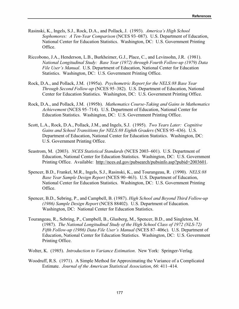
References
Rasinski, K., Ingels, S.J., Rock, D.A., and Pollack, J. (1993). America’s High School Sophomores: A Ten-Year Comparison (NCES 93–087). U.S. Department of Education, National Center for Education Statistics. Washington, DC: U.S. Government Printing Office.
Riccobono, J.A., Henderson, L.B., Burkheimer, G.J., Place, C., and Levinsohn, J.R. (1981). National Longitudinal Study: Base Year (1972) through Fourth Follow-up (1979) Data File User’s Manual. U.S. Department of Education, National Center for Education Statistics. Washington, DC: U.S. Government Printing Office.
Rock, D.A., and Pollack, J.M. (1995a). Psychometric Report for the NELS:88 Base Year Through Second Follow-up (NCES 95–382). U.S. Department of Education, National Center for Education Statistics. Washington, DC: U.S. Government Printing Office.
Rock, D.A., and Pollack, J.M. (1995b). Mathematics Course-Taking and Gains in Mathematics Achievement (NCES 95–714). U.S. Department of Education, National Center for Education Statistics. Washington, DC: U.S. Government Printing Office.
Scott, L.A., Rock, D.A., Pollack, J.M., and Ingels, S.J. (1995). Two Years Later: Cognitive Gains and School Transitions for NELS:88 Eighth Graders (NCES 95–436). U.S. Department of Education, National Center for Education Statistics. Washington, DC: U.S. Government Printing Office.
Seastrom, M. (2003). NCES Statistical Standards (NCES 2003–601). U.S. Department of Education, National Center for Education Statistics. Washington, DC: U.S. Government Printing Office. Available: http://nces.ed.gov/pubsearch/pubsinfo.asp?pubid=2003601.
Spencer, B.D., Frankel, M.R., Ingels, S.J., Rasinski, K., and Tourangeau, R. (1990). NELS:88 Base Year Sample Design Report (NCES 90–463). U.S. Department of Education, National Center for Education Statistics. Washington, DC: U.S. Government Printing Office.
Spencer, B.D., Sebring, P., and Campbell, B. (1987). High School and Beyond Third Follow-up (1986) Sample Design Report (NCES 88402). U.S. Department of Education. Washington, DC: National Center for Education Statistics.
Tourangeau, R., Sebring, P., Campbell, B., Glusberg, M., Spencer, B.D., and Singleton, M. (1987). The National Longitudinal Study of the High School Class of 1972 (NLS-72) Fifth Follow-up (1986) Data File User’s Manual (NCES 87–406c). U.S. Department of Education, National Center for Education Statistics. Washington, DC: U.S. Government Printing Office.
Wolter, K. (1985). Introduction to Variance Estimation. New York: Springer-Verlag.
Woodruff, R.S. (1971). A Simple Method for Approximating the Variance of a Complicated Estimate. Journal of the American Statistical Association, 66: 411–414.
177

References
Zahs, D., Pedlow, S., Morrissey, M., Marnell, P., and Nichols, B. (1995). High School and Beyond Fourth Follow-up Methodology Report (NCES 95–426). U.S. Department of Education, National Center for Education Statistics. Washington, DC: U.S. Government Printing Office.
178