sample analysis design - university of notre dameasimonet/engv60500/fall2012/... · sample analysis...

Sample Analysis Design

Solution Mode

Sample Analysis Design – Step I – Sample preparation

•  The quality of your data will only be as good as the ‘quality’ of your sample –

–  i.e. did you adequately prepare your sample in the clean lab?

–  With respect to the destruction of matrices for samples requiring digestion

–  Did you adequately spike samples with the correct internal standard?

–  Sample handling protocol is extremely important, e.g. weighing

Sample Analysis Design – Solid Samples

•  Analyze in solid state via LA-ICP-MS?

•  Analyze in solid state via SIMS – secondary ion mass spectrometry?

•  Convert into a glass bead and analyze via XRF – x-ray fluoresence?

•  Take powder and digest into solution with acids?

Sample Analysis Design- Liquid (aqueous) samples

–  run as-is?

–  filter then run?

– dilute then run?

– acidify, dilute, then run?

Sample Analysis Design •  Method of sample preparation also depends upon the

elements of interest

•  e.g. don’t analyze your samples in a hydrofluoric acid medium if you wish to measure Si abundances – why?

•  Elemental concentration determinations at ultra-trace level (ppb, ppt) are very susceptible to contamination during sample preparation and therefore should be conducted in clean laboratory environments

Sample Analysis Design – Clean room environment

•  Laboratory ‘clean’ room is a facility in which the concentration of airborne particles is controlled to specified limits.

•  Eliminating sub-micron airborne contamination is a control-driven process since contaminants are generated by people, process, facilities and equipment. Hence, sub-micron particles must be continually removed from the air.


•  Typical office building air contains from 500,000 to 1,000,000 particles (0.5 microns or larger) per cubic foot of air.

•  A Class 100 cleanroom is designed to never allow more than 100 particles (0.5 microns or larger) per cubic foot of air. Class 1000 and Class 10,000 cleanrooms are designed to limit particles to 1000 and 10,000, respectively


•  A human hair is about 75-100 microns in diameter. A particle 200 times smaller (0.5 micron) than the human hair can cause major disaster in a clean room.

•  Human hair typically concentrates elements/contaminants such as Pb!

Sample Analysis Design - Sources of contamination

•  Facilities: – Walls, floors and ceilings – Paint and coatings – Construction material (sheet rock, saw dust

etc.) – Air conditioning debris – Room air and vapors – Spills and leaks

Sample Analysis Design - Sources of contamination

•  People:

– Skin flakes and oil – Cosmetics and perfume – Spittle – Clothing debris (lint, fibers etc.) – Hair

Sample Analysis Design - Contamination Control

•  HEPA (High Efficiency Particulate Air Filter) - Extremely important for reducing contamination - filter particles as small as 0.3 microns with a 99.97% minimum particle-collective efficiency.

•  Clean room design – requires air flow dynamics to be the least disruptive as possible – laminar flow

•  Cleaning!

Sample Analysis Design - Contamination Control

•  Purity of reagents, acids, cleanliness of digestion vessels, sample bottles, etc can dramatically effect background levels and data quality

•  If possible, use highest purity commercial acids

•  At the minimum - sometimes need to further process reagents – e.g. acid distillation in our laboratory

•  Digestion vessels made of disposable fluorinated polymers (teflon, PFTE, PFA, etc)

•  Solutions stored in polypropylene or equivalent

Sample Analysis Design – Concentration terminology

•  Concentrations are typically expressed as either µg/g, or µg/ml (1 µg - microgram = 1 x 10-6 grams), or ppm, ppb, ppt

–  ppm = parts per million = 1 x 10-6 g/g = 1 µg/g –  (µg = microgram)

–  ppb = parts per billion = 1 x 10-9 g/g = 1 ng/g –  (ng = nanogram)

–  ppt = parts per trillion = 1 x 10-12 g/g = 1 pg/g –  (pg = picogram)


•  E.g. Zircon – ZrSiO4

–  ZrO2 = 67.2 wt% –  SiO2 = 32.8 wt%

–  Atomic mass of Zr= 91.224 –  Atomic mass of Si= 28.0855 –  Atomic mass of O= 15.9994

–  % Zr in ZrO2 = 91.224/(91.224 + (15.9994*2)) = 74 –  % Si in SiO2 = 28.0855/(28.0855 + (15.9994*2)) = 46.7


•  If 100% = 1,000,000 ppm, then

•  74% Zr (out of 67.2 wt%) = 49.73% or 497,300 ppm (or µg/g)

•  46.7% Si (out of 32.8 wt%) = 15.32% or 153,200 ppm (or µg/g)

•  If you are asked to weigh out 0.00001 g of zircon, then the amounts of total Zr and Si you would have are:

–  Zr = 497,300 µg/g x 0.00001 g = 4.97 µg –  Si = 153,200 µg/g x 0.00001 g = 1.53 µg


•  However, you are asked to prepare a solution of this zircon sample for ICP-MS analysis in solution mode;

•  then what would be the minimum dilution factor required given that the maximal amount of ion signal intensity allowed is 50 x 106 cps and the yield for both elements in medium resolution mode is ~60,000 cps/ppb?


•  Maximum allowable concentration is –

•  = Max. count rate/ yield = 50 x 106 cps/ 60,000 cps/ppb

•  = 833 ppb (ng/g)

•  4.97 µg of Zr needs to be diluted into ? ml of 5% HNO3.

–  4.97 µg = 4970 ng/833 ng/g = ~5.97 g (ml) of 5% HNO3

Sample Analysis Design – Matrix

•  Requires a medium (i.e. acid) that

–  Provides efficient ion transmission (HNO3 > HCl > H2O)

–  Won’t dissolve the glassware of your introduction system – for example, hydrofluoric acid (HF) would!

–  Is relatively cheap and not deemed extremely hazardous to use

–  Thus, dilute (1 to 5% volumetric) nitric acid (HNO3) is the acid medium of choice for most ICP-MS analyses

Sample Analysis Design – Step 2 – Calibration/Standard Preparation

•  Choice of calibration method dependent upon several factors:

•  1. potential matrix effects

•  2. number of samples

•  3. consistency of matrix across samples


•  EXTERNAL CALIBRATION: •  Prepare a set of standard solutions to cover the

expected range of analyte concentrations

•  Fit a least squares regression line

•  y = mx + b and calculate analyte concentration in unknowns


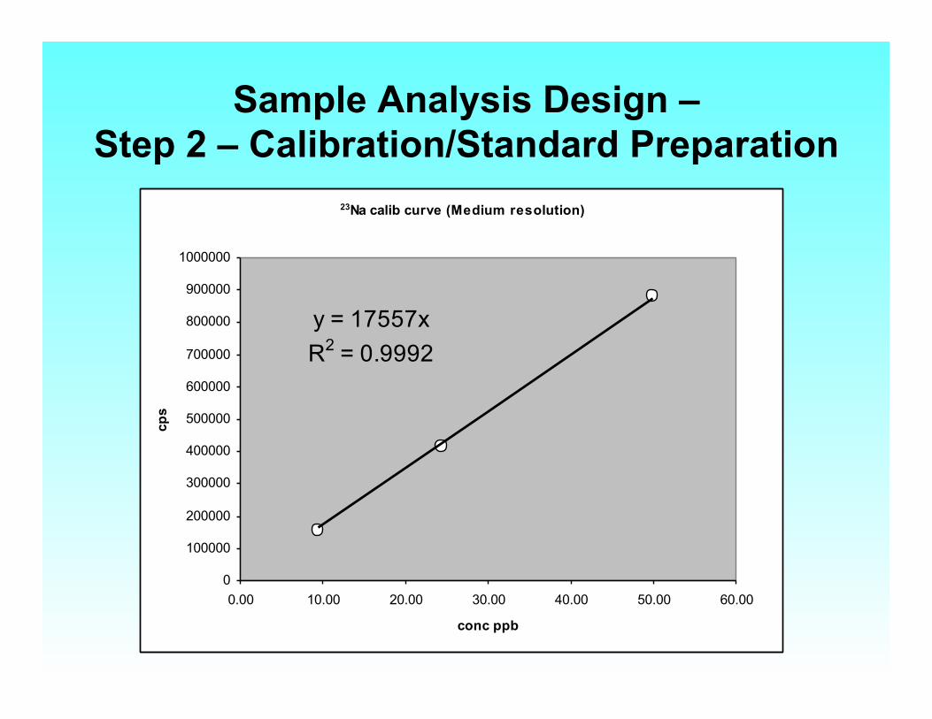
23Na calib curve (Medium resolution)

y = 17557xR2 = 0.9992

0

100000

200000

300000

400000

500000

600000

700000

800000

900000

1000000

0.00 10.00 20.00 30.00 40.00 50.00 60.00

conc ppb

cps


44Ca calib curve (Medium resolution)

y = 676.92xR2 = 0.9961

0

5000

10000

15000

20000

25000

30000

35000

40000

0.00 10.00 20.00 30.00 40.00 50.00 60.00

conc ppb

cps


•  Advantages of External Calibration

– Easy to prepare

– Quick

– Widely used technique

Sample Analysis Design – Step 2 – Calibration/Standard Preparation •  Disadvantages of External Calibration:

•  Need to matrix match calibration solutions and samples

•  If standards containing <2000 ug/ml (ppm) are being used, then preparing the standards as simple aqueous solutions using the acid matrix (5% HNO3) employed for the samples is sufficient

•  HOWEVER, if the samples contain a very high concentration of one (or more) elements, then this may not be adequate

Sample Analysis Design – Step 2 – Calibration/Standard Preparation •  Preparation of External Calibration Solutions:

•  Need to evenly space calibration concentrations

•  If the highest concentration is much higher than the rest, linear regression introduces bias favoring the high point

•  X = independent variable = concentration

•  Y = dependent variable = counts/second

Sample Analysis Design – Standard Addition Method

•  Aliquots of spike are added to unknown samples to increase the ion signal intensities for elements of interest

•  Typically use at least three aliquots of sample spiked with evenly spaced amounts of analyte

•  These spiked aliquots of sample are used to generate a calibration line and calculate the concentration in the sample


•  S0 = unspiked sample

•  S1 = sample spiked with analyte at concentration x

•  S2 = sample spiked with analyte at concentration 2x

•  S3 = sample spiked with analyte at concentration 3x

•  S4 = so on and so on


AMT

y = 29387x + 279235R2 = 0.9992

0

50000

100000

150000

200000

250000

300000

350000

400000

450000

500000

0 1 2 3 4 5 6 7

Concentration (ppb)

Cps


•  The concentration of the unknown solution is then determined by dividing the y-intercept value by the slope of the sample-spike mixing line.

–  From example on previous slide,

–  Conc. sol’n = 279235 / 29387 = 9.5 ppb

–  If the original sample was a solution, then this is the concentration of the analyte in question in the solution


•  If the original sample was in solid form that you digested and subsequently converted into a solution;

•  then in order to determine the concentration of the analyte in question, you must factor in the amount of total analyte in the solution and the dry weight of the sample powder


•  If we continue with the same example, the solution has a concentration of 9.5 ppb, and the original volume of the unknown solution was 10 ml (g) prior to aspirating some of it into the plasma for analysis, then the total amount analyte in the solution is:

•  = 10 g x 9.5 ng/g (ppb) •  = 95 ng, or •  = 0.095 µg

•  If the amount of powder weighed out was 0.1 g, then the concentration of the element in question is:

•  Conc. = 0.095 µg/0.1 g –  = 0.95 µg/g or ppm


•  This method works best if the slope of the calibration line is not too shallow

– This will create more uncertainty in the location of the intersection between the cps of your unknown and the calibration line


•  For maximum precision it’s necessary that the amount of sample be the same in each aliquot

•  Also want the amount of spike added to be the same for each aliquot

•  Amount of spike added should be as small as possible (usually 0.1 ml to 10 ml total volume)


•  Ideally, the highest spike concentration should be approximately equal to the concentration of analyte in the unknown

•  Need to have some idea of the concentration in the sample prior to analysis


•  Advantages:

–  Overcomes matrix differences –  More precise and accurate than external calibration

•  Disadvantages:

–  Requires at least three aliquots for each sample –  Run lengths become much longer and more

preparation time is required

Sample Analysis Design – Isotope Dilution

•  Most accurate and precise calibration method available

•  Requires analyte with two stable isotopes

•  Monoisotopic elements cannot be determined via isotope dilution

•  Spike natural sample with enriched isotope spike of analyte


•  The amount of spike is selected so that the resulting ratio between spiked isotope and unspiked isotope is near unity – maximizes precision

•  Typically use the most abundant isotope as the reference -- maximizes sensitivity


•  Check isotope ratio in unspiked sample to determine if the “natural ratio” in the sample matches with the predicted ratio

•  If not -- interference in acting on one or both of the isotopes

•  Always attempt to use interference free isotopes


•  Prepare the spike to desired concentration

•  Add spike as early as possible – after equilibration of spike and sample you don’t have to have complete sample recovery

•  During any stage of the process complete equilibration is absolutely necessary


•  Analyze the solution on the ICP using many repetitive scans (to maximize precision)

•  Need to measure isotopic ratios on standards of a known ratio in order to correct for machine mass discrimination

•  Use previous equation to calculate concentrations!


•  Advantages:

–  Most accurate and precise method for quantitative elemental concentrations

–  Partial loss of analyte during preparation is compensated for since physical and chemical interferences are not an issue -- will cancel out as they will affect each isotope identically

–  Ideal form of internal standardization since another isotope of the same element is used in this capacity



– Generally only applicable to multiple-isotopic elements

– Need an enriched isotope spike for the analyte of interest - not always available or sometimes at very high cost

– Need two interference free isotopes – VERY time consuming

Sample Analysis Design

STEP 3 – INTERNAL STANDARDIZATION & INSTRUMENT

DRIFT CORRECTION

Sample Analysis Design – Internal Standard

•  Every sample should be analyzed with an internal standard (IS)

•  What is an internal standard (IS)?

–  element that is added to EVERY sample/ blank/calibration standard/QA sample/etc., that is not expected to be in the sample in appreciable quantities and is not an element of interest

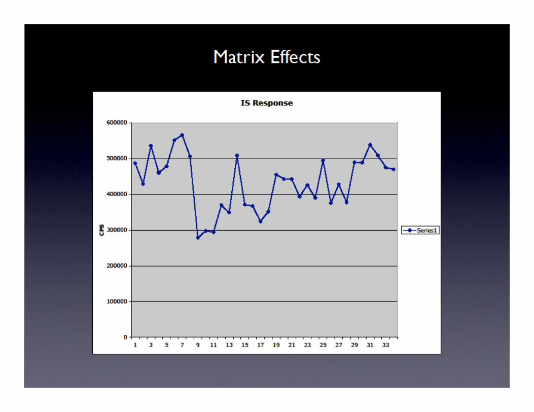
–  use IS to monitor machine drift (both short and long term) and matrix effects


•  Choice of IS depends upon which elements you are quantifying

•  The IS should have similar properties in the plasma as element(s) of interest

•  ICP-MS: similar in mass/ionization potential


•  Example:

–  attempting to quantify U - use Th

–  attempting to quantify most transition metals - use As

–  attempting to quantify REEs - use Re

–  115In and 103Rh are common IS for general use

–  alternatively, you can add several IS to each sample


•  From previous slide, we assume that samples have little or no Th, As, or Re

•  It’s important to have an idea of what’s in your sample prior to quantitative analysis

•  Solid samples can use a naturally occurring element as IS, provided that you know the concentration in each sample


•  Procedure for IS use:

•  Calculate the concentration of the IS in each centrifuge tube – the latter will contain an aliquot of your sample and an aliquot of the IS

•  Divide the measured ion signal (CPS) by the concentration of your IS to derive the factor = CPS/ppb

•  Divide CPS/ppb of each tube by the CPS/ppb for those measured for the blanks since these are not influenced by possible effects due to sample matrices

•  The latter yields a dimensionless correction factor (I refer to it as a normalization factor)

•  Use correction factor to adjust analyte counts for drift or matrix effects


•  Advantages:

•  Fluctuations are monitored in each sample/ calibration / blank


•  Assume that behavior of IS is the same as the analyte

Sample Analysis Design – Instrumental Drift

•  Correct for instrument drift with:

•  Internal standardization is a common procedure

•  Use of drift corrector solutions (DCS)


•  Drift Corrector Solutions (DCS):

•  Measure the same solution intermittently throughout the course of the analytical session

•  Change in ion signal is assumed to be linear between each DCS measurement


•  The DCS should contain all elements of interest and can be matrix matched to samples

– Example: use standard reference materials (SRMs) for DCS


•  Apply a linear correction to samples between DCS solutions

•  DCS1 + ((DCS2 - DCS1)*F)

•  F = position dependent fraction


•  Advantages of DCS correction:

–  all analytes are monitored for drift

–  nothing added to sample solutions

•  Disadvantages of DCS correction:

–  assume change is linear

–  cannot easily monitor matrix effects

Sample Analysis Design – Background & blanks

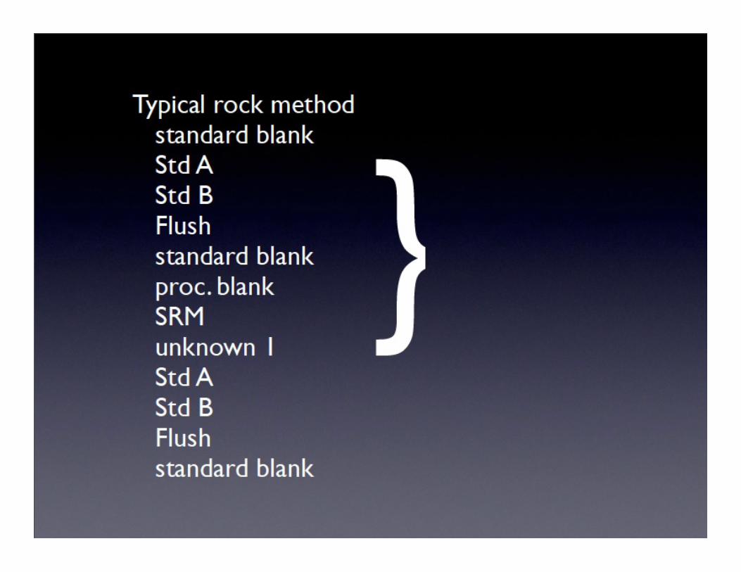
•  Standard blank - blank used to monitor polyatomic ion interferences, gas peaks, and contamination from reagents; used for background subtraction

•  Procedural blank - blank used to monitor contamination acquired during all stages of sample preparation; grinding, digestion, acidification, powdering, etc


•  Use of blanks during an analytical session:

•  ALWAYS begin an analytical session with at least one standard blank

•  Analyze standard blanks periodically throughout the course of the session in particular to monitor memory effects

•  Process and analyze at least one procedural blank at some point during your research study; for its analysis, it’s preferable to measure it early in order to avoid any potential memory effects


•  The more standard blanks that are run during an analytical session, the more information you will have with regards to monitoring change(s) in background levels throughout the entire session


•  How to determine “the background”:

•  1. just use the first standard blank

•  2. average all standard blanks

•  3. take median of all standard blanks

•  4. apply statistical analysis to standard blanks and select some of them


•  Outlier tests:

•  1. I know the truth

•  2. Looks different

•  3. Statistical “proof”


•  Option 1 should be avoided - unscientific and invalid

•  Option 2 is better but only if the measurement is repeated

•  Option 3 is the best approach, but needs to be carried out carefully in order to avoid false negatives and positives


•  Huber Outlier Test

•  take median of all values

•  calculate absolute deviation |xi - xm|

•  take mean of absolute deviations (MAD)

•  multiply MAD by coefficient (k = 3-5)

•  anything higher than k*MAD is rejected as outlier


•  Calculation of Limit of Detection (DL) and Limit of Quantification (QL)

•  Easy way: •  LOD = 3*STDEVblank; •  LOQ = 10*STDEVblank

Sample Analysis Design – SUMMARY

•  A ‘good’ analytical method will:

•  1. provide the means to calculate an accurate background level

•  2. allow for correction of instrument drift

•  3. use Internal standardization to monitor matrix effects

•  4. provide some method for monitoring/ correcting interferences

•  5. Use a proper calibration strategy

sample analysis design - university of notre dameasimonet/engv60500/fall2012/... · sample analysis...

Documents