s42 dw 14 discard length v2 -...

Size Distribution of Red Grouper Observed in For-‐Hire Recreational Fisheries in the Gulf of Mexico

Alisha Gray and Beverly Sauls

SEDAR 42-‐DW-‐14

20 November 2014 Updated: 15 December 2014

This information is distributed solely for the purpose of pre-dissemination peer review. It does not represent and should not be construed to represent any agency determination or policy.

Please cite this document as: Gray, A. and B. Sauls. 2014. Size Distribution of Red Grouper Observed in For-Hire Recreational Fisheries in the Gulf of Mexico. SEDAR42-DW-14. SEDAR, North Charleston, SC. 22 pp.

1

Red Grouper Size Distribution and Standardized CPUE Observed in For-Hire Recreational Fisheries in the Gulf of Mexico Prepared by: Alisha Gray Florida Fish and Wildlife Conservation Commission Fish and Wildlife Research Institute Saint Petersburg, FL Beverly Sauls Florida Fish and Wildlife Conservation Commission Fish and Wildlife Research Institute Saint Petersburg, FL For: SEDAR 42 Eastern Gulf of Mexico Red Grouper Data Workshop, October, 2014. Detailed information on the size of discarded fish is not collected in traditional dockside surveys of recreational fisheries. At-sea observer surveys provide valuable information on the size and condition of discarded fish. Such surveys have been conducted on headboat vessels in the eastern Gulf of Mexico since 2005. Coverage was expanded in June of 2009 to include charter vessels on the east coast of Florida, and this coverage continued through 2013. This report provides a summary of available information on the size and catch-per-unit-effort for Red Grouper collected from headboats and charter boats from the Gulf coast of Florida. For detailed methods and results, refer also to Sauls et al. (2014), which was provided as a reference document for this data workshop (SEDAR42-RD01). Coverage Fishery observer coverage for headboats and charter boats operating on the Gulf coast of Florida is summarized in Table 1. From 2005-2007, at-sea observer surveys were conducted on headboats only from Alabama through Southwest Florida (Figure 1); however, funding was discontinued in 2008. A new funding source allowed coverage to resume on both headboats and charter boats over a reduced area (A, B and C in Figure 1 and Table 1) from June 2009 through December 2013. Table 1. Fishery observer coverage for headboats (H) and charter vessels (C) on the Gulf coast of Florida. Refer to figure 1 for areas. Area 2005 2006 2007 2008 2009* 2010 2011 2012 2013 NW panhandle (A) H H H H, C H, C H, C H, C H, C TB nearshore (B) H H H H, C H, C H, C H, C H, C TB offshore (C) H H H H H H H H Naples/Ft. Meyers (E) H H H *Sampling did not resume until June. Cooperative vessels were randomly selected year-round for observer coverage, and samples were stratified by region (Figure 1). Operators from selected vessels were contacted by state biologists and one or two observers were scheduled to sample a single trip in a selected week. Monthly

2

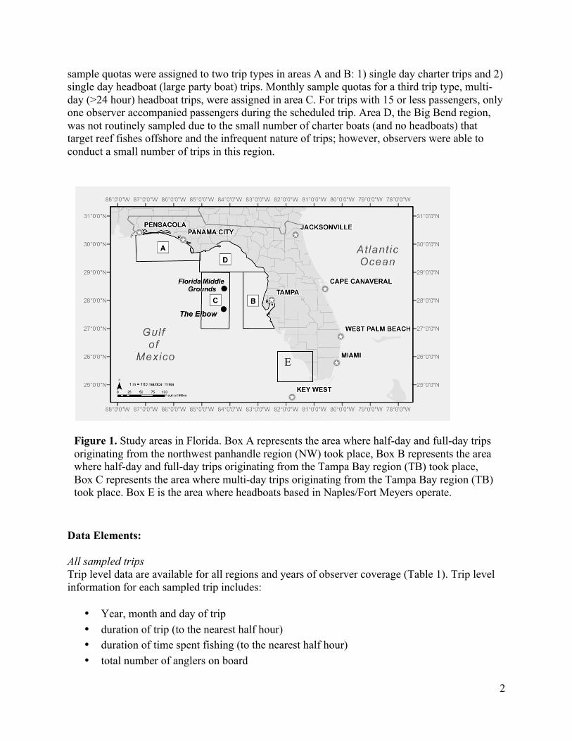
sample quotas were assigned to two trip types in areas A and B: 1) single day charter trips and 2) single day headboat (large party boat) trips. Monthly sample quotas for a third trip type, multi-day (>24 hour) headboat trips, were assigned in area C. For trips with 15 or less passengers, only one observer accompanied passengers during the scheduled trip. Area D, the Big Bend region, was not routinely sampled due to the small number of charter boats (and no headboats) that target reef fishes offshore and the infrequent nature of trips; however, observers were able to conduct a small number of trips in this region.

Data Elements: All sampled trips Trip level data are available for all regions and years of observer coverage (Table 1). Trip level information for each sampled trip includes:

• Year, month and day of trip • duration of trip (to the nearest half hour) • duration of time spent fishing (to the nearest half hour) • total number of anglers on board

Figure 1. Study areas in Florida. Box A represents the area where half-day and full-day trips originating from the northwest panhandle region (NW) took place, Box B represents the area where half-day and full-day trips originating from the Tampa Bay region (TB) took place, Box C represents the area where multi-day trips originating from the Tampa Bay region (TB) took place. Box E is the area where headboats based in Naples/Fort Meyers operate.

E

3

• number of anglers observed • minimum and maximum depths fished

For each location fished during a sampled trip, the following station-level information was recorded:

• latitude and longitude (degrees and minutes) • fishing zone and subzone (same as commercial zones) • bottom depth (meters) • up to three target species and percentage of time targeting each

For each angler observed during a sampled trip, the following information was collected: • total number of fish retained by species • total number of fish discarded alive by species • total number of fish discarded dead by species

For each rod fished by an observed angler at a given station, the following information was recorded:

• leader type and strength • hook type (circle hook, J hook, kahle hook, treble hook, other) • hook offset (yes or no) • hook size (using a standard hook sizing chart) • bait type (live, whole dead fish, cut fish, squid, cocktail, artificial)

For each fish observed from a given rod at a given station, the following information was recorded:

• species • mid-line length (mm) • disposition, coded as:

o 1: thrown back alive, legal o 2: thrown back alive, not legal o 3: plan to eat o 4: used for bait or plan to use for bait o 5: sold or plan to sell o 6: thrown back dead or plan to throw away o 7: other

• method of hook removal (easy or difficult; by hand, dehooking tool, pliers, or left in place)

• presence of barotrauma symptoms (inflated bladder, everted stomach, extruded intestines, exopthalmia)

• venting method (released without venting, bladder vented, stomach vented) • presence of gill injury (visible bleeding from gills)

4

Sample Weights for Size Distribution: To generate weighting factors for different trip-types, fishing effort data for the years 2009 through 2013 were used to calculate proportional effort by trip-type. Headboat vessels report fishing effort in logbook trip reports, and effort data from the two study regions in the Gulf of Mexico were provided by the NMFS Southeast Fisheries Science Center in Beaufort, NC. Effort data for charter vessels is collected through the For-Hire Survey component of the Marine Recreational Information Program, which a weekly vessel directory telephone survey of charter boat operators (Van Voorhees et al. 2002). Proportional fishing effort was calculated as the total numbers of trips in the Gulf of Mexico reported for a given trip-type divided by the total number of Gulf trips reported. To obtain the sample weight (Wt), proportional effort was then divided by the proportion of a given trip type in the sample population: Wt = (Nt/N) / (nt/n) Equation 1 Where Nt /N is the number of trips of type t divided by total trips reported, and nt/n is the number of trips of type t in the sample population divided by the total number of sampled trips. Trip-types with Wt < 1 are down weighted to account for oversampling and trip-types with Wt > 1 are inflated to account for undersampling. Numbers of charter and headboat trips sampled per year are provided in Table 2.1 and 2.2. Total number of fish sampled on headboats for this project are given in Table 3.1, while number sampled on charter vessels are given in Table 3.2. Sample weights are provided in Table 4.1 and 4.2. Headboat trip type (e.g., half day, full day, etc.) was recorded differently in 2013 compared to prior years; however, trip type was standardized across all years to produce the sample weights provided here. Finally, a distribution of sampled trips by trip duration per year is given in Figure 2.1 and 2.2. Table 2.1. Numbers of headboat trips sampled each year by region. Regions shaded in gray represent the area with most consistent coverage throughout the time series. Area 2005 2006 2007 2008 2009 2010 2011 2012 2013 Alabama 48 55 37 NW FL (A) 55 46 52 28 32 52 49 39 TB FL (B-C) 53 64 63 35 49 48 44 48 SW FL (D) 36 39 26 Table 2.2. Charter at-sea observer trips sampled per year.

Year Trips 2009 32 2010 52 2011 70 2012 58 2013 52

5

Table 3.1. Sample sizes of Red Grouper length measurements from headboats. Year Disposition Region A Region B-C Total 2005 Discard 163 963 1126

Harvest 15 32 47

2006 Discard 54 1004 1058

Harvest 26 67 93

2007 Discard 19 1614 1633

Harvest 19 142 161

2009 Discard 27 1707 1734

Harvest 3 40 43

2010 Discard 21 1571 1592

Harvest 4 9 13

2011 Discard 33 1023 1056

Harvest 13 37 50

2012 Discard 19 616 635

Harvest 9 31 40

2013 Discard 8 764 772

Harvest 3 36 39

Table 3.2. Sample sizes of Red Grouper length measurements from charter boats. Year Disposition Region A Region B-C Total 2009 Discard 46 983 1029

Harvest 7 35 42

2010 Discard 145 2168 2313

Harvest 27 75 102

2011 Discard 76 1758 1834

Harvest 39 75 114

2012 Discard 16 1308 1324

Harvest 37 134 171

2013 Discard 5 1190 1195

Harvest 15 160 175

6

Table 4.1. Sample weights (Way) by year and trip type for Charter vessels. Region Year Half day 3/4 day Full day Multi-day

NW charter 2009 4.880992 0.759578 0.512414

2010 2.721536 0.601878 0.962257

2011 3.522423 0.562034 1.267357

2012 2.253355 0.620278 0.977800

2013 1.332341 0.754993 1.262676

TB charter 2009 9.409514 0.843459 0.203723

2010 2.199546 0.916811 0.378559 0.037793

2011 1.336384 1.071163 0.287683

2012 2.864030 0.679953 0.271719

2013 1.435865 0.655321 1.02407

Table 4.2. Sample weights (Way) by year and trip type for Headboat vessels.

Year Half day 3/4 day Full day Multi-day 2005 4.3929 0.8497 1.3905 0.0786 2006 2.6677 1.0168 0.8960 0.1097 2007 2.5789 0.9907 1.2222 0.0490 2009 4.5287 0.9898 0.3112 0.0676 2010 2.6680 1.0916 0.3111 0.0906 2011 1.5677 1.1018 0.6231 0.0643 2012 1.2124 1.2423 0.6996 0.0945 2013 1.0571 3.0613 0.8487 0.1001

7

Size Distribution of Discards Individual fish were assigned to one cm length bin categories (40 cm bin = fish 39.5 cm to 40.4 cm). The numbers of fish in each length bin category were summed by disposition (harvested, released), and multiplied by appropriate sample weights. Discard length distributions from head boats are shown in Figure 3 and discard length distributions from charter vessels are shown in Figure 4.

Figure 2. Distribution of sampled trips by trip type and year.

0% 20% 40% 60% 80%

100%

2005 2006 2007 2009 2010 2011 2012 2013

Perc

ent

Year

Headboat

Multi-da

Half day

Full day

3/4 day

0%

20%

40%

60%

80%

100%

2009 2010 2011 2012 2013

Perc

ent

Year

Charter

Multi-da

Half day

Full day

3/4 day

8

Figure 3. Weighted length frequencies (expressed as proportions) of red grouper discards from head boat vessels. The minimum size limit for harvest is 20” total length (50.8 cm TL).

0

0.02

0.04

0.06

0.08

0.1

0 10 20 30 40 50 60 70 80 90 Midline Length (cm)

2005

0

0.02

0.04

0.06

0.08

0.1


2006

9

Figure 3 continued

0

0.02

0.04

0.06

0.08

0.1


2007

0

0.02

0.04

0.06

0.08

0.1


2009

0

0.02

0.04

0.06

0.08

0.1


2010

10

Figure 3 continued

0

0.02

0.04

0.06

0.08

0.1


2011

0

0.02

0.04

0.06

0.08

0.1


2012

0

0.02

0.04

0.06

0.08

0.1


2013

11

Figure 4. Weighted length frequencies (expressed as proportions) of red grouper discards from charter vessels. The minimum size limit for harvest is 20” total length (50.8 cm TL).

0

0.02

0.04

0.06

0.08

0.1

10 20 30 40 50 60 70 80 90 100 110 120 Midline Length (cm)

2010

0

0.02

0.04

0.06

0.08

0.1


2011

0

0.02

0.04

0.06

0.08

0.1


2012

12

Standardized Catch-per-Unit-Effort (CPUE) Observer data were used to construct an index of abundance from standardized catch-per-unit effort data collected from headboats. The effort unit for this index was numbers of red grouper discards observed per angler hour. Methods Harvested red grouper were excluded from this index to avoid overlap with other fisheries-dependent indices that measure abundance of legal-sized harvested fish and provide a longer time series. Only single day headboat trips sampled from the two regions with the most consistent observer coverage throughout the time series were included in this index (Table 2.1). Other regions in Florida and Alabama that have had inconsistent observer coverage are not included in this index. Multi-day trips from the Tampa Bay region (TB FL in Table 2.1) were also excluded since the majority of red grouper caught during these trips are legal sized. In the Tampa Bay region, red grouper were present on 89% of trips; therefore, all trips in this region were considered potential red grouper trips. In the Panhandle, no red grouper were observed from the majority of trips sampled (Table 5), and clustering methods were explored to determine the subset of trips from this region to include in an index. The Stephens and McCall (2004) method was explored; however, due to the frequency of false negatives (positive trips with a low estimated probability for red grouper presence), this was not a reliable method for identifying red grouper trips in the region. Hierarchical cluster analysis revealed close association between red grouper and numerous reef associated fishes that are abundant in the panhandle (including vermilion snapper, red snapper, and porgies). The species composition for clustering was sensitive to Morisita and Horn-Morisita aggregation indices, and both methods included the most frequently caught species in the panhandle region (red snapper, vermilion, gray triggerfish, red porgy). So in both cases, no trips were dropped from consideration for a red grouper index. Therefore, all single-day headboat trips sampled from the Tampa Bay and panhandle regions were included in this index, regardless of red grouper presence.

Figure 4. continued.

0

0.02

0.04

0.06

0.08

0.1


2013

13

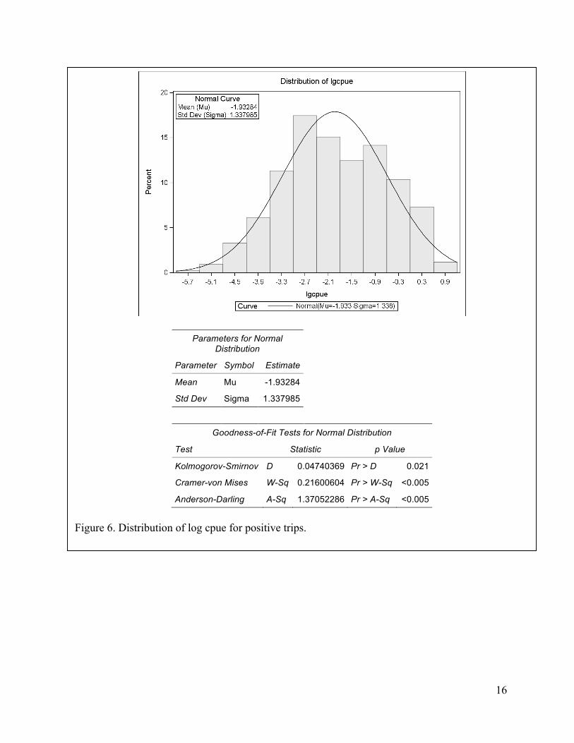
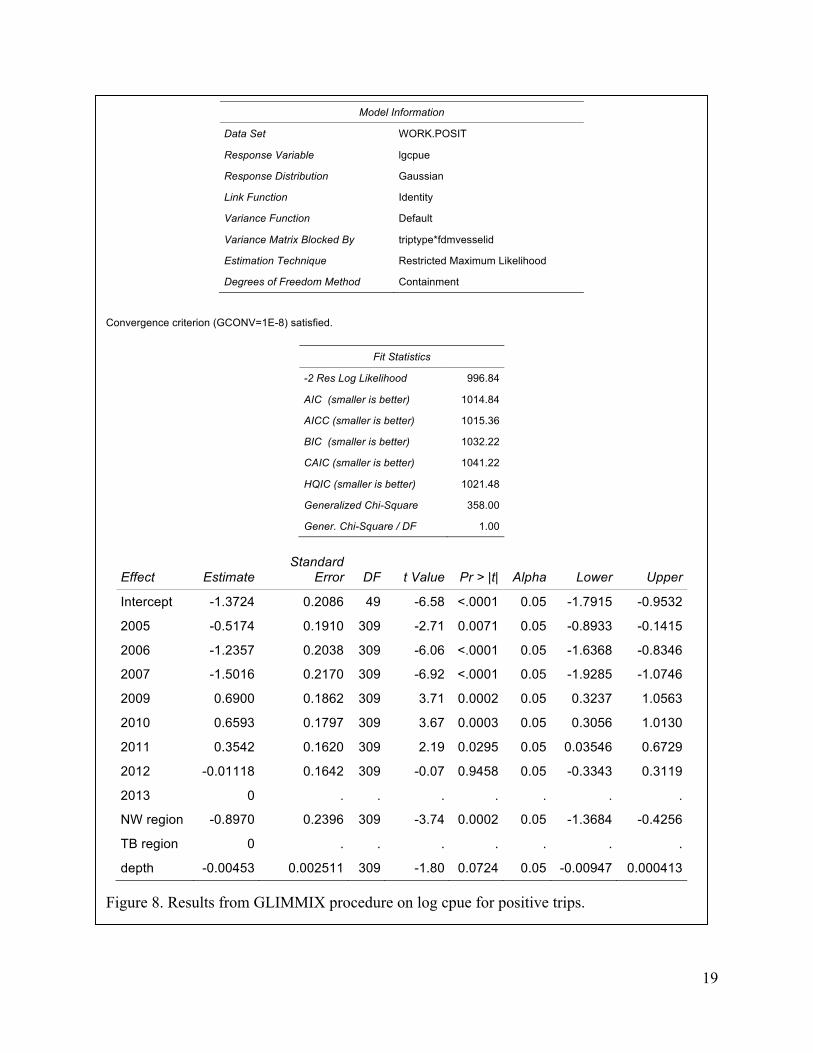
Separate GLMs were constructed for the binomial presence/absence of red grouper discards and CPUE for positive trips (expressed as the log of discards per observed angler hour). The GLMs were constructed using the GLIMMIX procedure in SAS. A total of 33 unique headboat vessels were sampled repeatedly throughout the time series, and CPUE is likely correlated with the region where individual vessels operate from, patterns in the types of trips offered, locations vessel operators choose to fish, and other potential factors. Correlation within repeated observations on the same vessels was accounted for with a generalized estimating equation (GEE) using the random statement in GLIMMIX. To insure that similar types of trips were clustered together, clusters were defined by vessel and trip type, with trip types defined as half-day (<6 hours), three-quarter-day (6 to <9 hours), or full day (9 hours or longer). Year and region were included as covariates in the model. One other covariate, depth fished, improved the model fit but was not included due to missing values for a large portion of trips in one year (2007) that impacted sample size. Results Nominal CPUE (measured as catch per observed angler-hour) by year is provided in Table 5. Figures 5 and 6 summarize the distribution of proportion positive trips and CPUE for positive trips. Results for the binomial and lognormal models are provided in Figures 7 and 8. Results for the standardized index of abundance are provided in Figure 9.

14

Table 5. Frequency of total and positive trips (N_obs and N_pp), proportion positive trips (PP_obs), and nominal catch per observed angler hour (mean_CPUE).

Factor Level N_OBS N_PP PP_OBS Mean_CPUE

YEAR 2005 90 62 0.68889 0.09984

YEAR 2006 103 56 0.54369 0.04027

YEAR 2007 107 60 0.56075 0.08977

YEAR 2009 62 43 0.69355 0.38711

YEAR 2010 78 49 0.62821 0.41891

YEAR 2011 103 59 0.57282 0.25459

YEAR 2012 92 47 0.51087 0.15249

YEAR 2013 88 48 0.54545 0.18316

flreg NW 348 92 0.26437 0.01751

flreg TB 375 332 0.88533 0.34585

YEAR 2005 90 62 0.68889 0.09984

YEAR 2006 103 56 0.54369 0.04027

YEAR 2007 107 60 0.56075 0.08977

YEAR 2009 62 43 0.69355 0.38711

YEAR 2010 78 49 0.62821 0.41891

YEAR 2011 103 59 0.57282 0.25459

YEAR 2012 92 47 0.51087 0.15249

YEAR 2013 88 48 0.54545 0.18316

flreg NW 348 92 0.26437 0.01751

flreg TB 375 332 0.88533 0.34585

15

YEAR OF DATA N Mean Std Dev Minimum Maximum

2005 6 0.6343776 0.3635292 0.1428571 1.0000000

2006 6 0.5210573 0.3514806 0.0833333 1.0000000

2007 6 0.5503350 0.3469643 0.1666667 1.0000000

2009 5 0.6750000 0.4643544 0 1.0000000

2010 6 0.5755952 0.4415905 0.1250000 1.0000000

2011 6 0.6566783 0.3577519 0.1707317 1.0000000

2012 6 0.6893143 0.4603655 0.0833333 1.0000000

2013 6 0.5178571 0.5296081 0 1.0000000

Figure 5. Distribution of percent positive trips by year, region and trip type.

16

Parameters for Normal Distribution

Parameter Symbol Estimate

Mean Mu -1.93284

Std Dev Sigma 1.337985

Goodness-of-Fit Tests for Normal Distribution

Test Statistic p Value

Kolmogorov-Smirnov D 0.04740369 Pr > D 0.021

Cramer-von Mises W-Sq 0.21600604 Pr > W-Sq <0.005

Anderson-Darling A-Sq 1.37052286 Pr > A-Sq <0.005

Figure 6. Distribution of log cpue for positive trips.

17

Model Information

Data Set WORK.ANALYSIS

Response Variable success

Response Distribution Binomial

Link Function Logit

Variance Function Default

Variance Matrix Blocked By triptype*fdmvesselid

Estimation Technique Residual PL

Degrees of Freedom Method Kenward-Roger

Fixed Effects SE Adjustment Kenward-Roger

Solutions for Fixed Effects

Effect triptype

YEAR OF DATA flreg Estimate

Standard Error DF t Value Pr > |t| Alpha Lower Upper

Intercept 2.1892 0.4141 101.6 5.29 <.0001 0.05 1.3678 3.0105

YEAR 2005 0.8222 0.3981 700 2.07 0.0393 0.05 0.04054 1.6039

YEAR 2006 -0.7614 0.3836 704.3 -1.98 0.0475 0.05 -1.5144 -0.00830

YEAR 2007 -0.4404 0.3856 708.3 -1.14 0.2538 0.05 -1.1974 0.3166

YEAR 2009 0.7413 0.4377 691.9 1.69 0.0908 0.05 -0.1181 1.6007

YEAR 2010 -0.2164 0.4260 708.2 -0.51 0.6117 0.05 -1.0527 0.6200

YEAR 2011 0.4015 0.3706 690.1 1.08 0.2790 0.05 -0.3261 1.1292

YEAR 2012 0.03905 0.3713 674.9 0.11 0.9163 0.05 -0.6899 0.7680

YEAR 2013 0 . . . . . . .

triptype Full 2.0336 0.4760 45.92 4.27 <.0001 0.05 1.0754 2.9919

triptype Half -0.9058 0.3764 29.52 -2.41 0.0226 0.05 -1.6751 -0.1365

triptype Three-quarter

0 . . . . . . .

flreg 1 -3.5484 0.3474 35.96 -10.21 <.0001 0.05 -4.2530 -2.8438

flreg 2 0 . . . . . . .

Type III Tests of Fixed Effects

Effect Num

DF Den DF Chi-Square F Value Pr > ChiSq Pr > F

YEAR 7 703 26.27 3.75 0.0004 0.0005

triptype 2 38.36 30.77 15.37 <.0001 <.0001

flreg 1 35.96 104.31 104.31 <.0001 <.0001

Figure 7. Results of the GLIMMIX procedure for bi-nomial proportion positive trips.

18

YEAR Least Squares Means

YEAR OF DATA Estimate

Standard Error DF t Value Pr > |t| Alpha Lower Upper Mean

Standard Error

Mean Lower Mean

Upper Mean

2005 1.6131 0.3184 237.5 5.07 <.0001 0.05 0.9858 2.2405 0.8338 0.04412 0.7283 0.9038

2006 0.02953 0.2947 184.8 0.10 0.9203 0.05 -0.5519 0.6110 0.5074 0.07366 0.3654 0.6482

2007 0.3505 0.3009 218.3 1.16 0.2454 0.05 -0.2425 0.9436 0.5867 0.07296 0.4397 0.7198

2009 1.5322 0.3847 454.1 3.98 <.0001 0.05 0.7761 2.2883 0.8223 0.05621 0.6848 0.9079

2010 0.5745 0.3479 255.6 1.65 0.0998 0.05 -0.1105 1.2596 0.6398 0.08017 0.4724 0.7790

2011 1.1924 0.3072 223.5 3.88 0.0001 0.05 0.5870 1.7979 0.7672 0.05488 0.6427 0.8579

2012 0.8299 0.3143 218.2 2.64 0.0089 0.05 0.2105 1.4494 0.6963 0.06646 0.5524 0.8099

2013 0.7909 0.3272 263 2.42 0.0163 0.05 0.1465 1.4352 0.6880 0.07024 0.5366 0.8077

Figure 7 (continued).

obppos

0.0

0.1

0.2

0.3

0.4

0.5

0.6

0.7

0.8

0.9

YEAR OF DATA

2005 2006 2007 2008 2009 2010 2011 2012 2013

FWC Headboat Observer Red Grouper Gulf of Mexico 2005 to 2013Diagnostic plots: 1) Obs vs Pred Proport Posit

PLOT obppos bc_pos

19

Model Information

Data Set WORK.POSIT

Response Variable lgcpue

Response Distribution Gaussian

Link Function Identity

Variance Function Default

Variance Matrix Blocked By triptype*fdmvesselid

Estimation Technique Restricted Maximum Likelihood

Degrees of Freedom Method Containment

Convergence criterion (GCONV=1E-8) satisfied.

Fit Statistics

-2 Res Log Likelihood 996.84

AIC (smaller is better) 1014.84

AICC (smaller is better) 1015.36

BIC (smaller is better) 1032.22

CAIC (smaller is better) 1041.22

HQIC (smaller is better) 1021.48

Generalized Chi-Square 358.00

Gener. Chi-Square / DF 1.00

Effect Estimate Standard

Error DF t Value Pr > |t| Alpha Lower Upper

Intercept -1.3724 0.2086 49 -6.58 <.0001 0.05 -1.7915 -0.9532

2005 -0.5174 0.1910 309 -2.71 0.0071 0.05 -0.8933 -0.1415

2006 -1.2357 0.2038 309 -6.06 <.0001 0.05 -1.6368 -0.8346

2007 -1.5016 0.2170 309 -6.92 <.0001 0.05 -1.9285 -1.0746

2009 0.6900 0.1862 309 3.71 0.0002 0.05 0.3237 1.0563

2010 0.6593 0.1797 309 3.67 0.0003 0.05 0.3056 1.0130

2011 0.3542 0.1620 309 2.19 0.0295 0.05 0.03546 0.6729

2012 -0.01118 0.1642 309 -0.07 0.9458 0.05 -0.3343 0.3119

2013 0 . . . . . . .

NW region -0.8970 0.2396 309 -3.74 0.0002 0.05 -1.3684 -0.4256

TB region 0 . . . . . . .

depth -0.00453 0.002511 309 -1.80 0.0724 0.05 -0.00947 0.000413 Figure 8. Results from GLIMMIX procedure on log cpue for positive trips.

20

Type III Tests of Fixed Effects

Effect Num

DF Den DF Chi-Square F Value Pr > ChiSq Pr > F

YEAR 7 309 189.21 27.03 <.0001 <.0001

flreg 1 309 14.02 14.02 0.0002 0.0002

DEPTH_SH 1 309 3.25 3.25 0.0714 0.0724

YEAR Estimate Standard

Error DF t Value Pr > |t| Alpha Lower Upper Mean

Standard Error

Mean Lower Mean

Upper Mean

2005 -2.4025 0.1605 309 -14.97 <.0001 0.05 -2.7182 -2.0868 -2.4025 0.1605 -2.7182 -2.0868

2006 -3.1208 0.1761 309 -17.73 <.0001 0.05 -3.4672 -2.7744 -3.1208 0.1761 -3.4672 -2.7744

2007 -3.3867 0.1975 309 -17.15 <.0001 0.05 -3.7753 -2.9981 -3.3867 0.1975 -3.7753 -2.9981

2009 -1.1951 0.1610 309 -7.42 <.0001 0.05 -1.5118 -0.8784 -1.1951 0.1610 -1.5118 -0.8784

2010 -1.2258 0.1602 309 -7.65 <.0001 0.05 -1.5411 -0.9105 -1.2258 0.1602 -1.5411 -0.9105

2011 -1.5309 0.1363 309 -11.23 <.0001 0.05 -1.7991 -1.2627 -1.5309 0.1363 -1.7991 -1.2627

2012 -1.8963 0.1494 309 -12.69 <.0001 0.05 -2.1902 -1.6023 -1.8963 0.1494 -2.1902 -1.6023

2013 -1.8851 0.1516 309 -12.44 <.0001 0.05 -2.1833 -1.5869 -1.8851 0.1516 -2.1833 -1.5869

Obs YEAR cpue lcpu selcpu mc margPos vposcatch cvposcatch

1 2005 0.09166 -2.40250 0.16046 309 WORK.POSIT 0.025746 -0.06679

2 2006 0.04481 -3.12081 0.17606 309 WORK.POSIT 0.030998 -0.05642

3 2007 0.03449 -3.38669 0.19748 309 WORK.POSIT 0.039000 -0.05831

4 2009 0.30662 -1.19510 0.16097 309 WORK.POSIT 0.025911 -0.13469

5 2010 0.29732 -1.22580 0.16025 309 WORK.POSIT 0.025679 -0.13073

6 2011 0.21836 -1.53091 0.13631 309 WORK.POSIT 0.018581 -0.08904

7 2012 0.15181 -1.89629 0.14939 309 WORK.POSIT 0.022318 -0.07878

8 2013 0.15357 -1.88511 0.15156 309 WORK.POSIT 0.022969 -0.08040

Figure 8 (continued).

obcppos

0.0

0.1

0.2

0.3

0.4

0.5

0.6

0.7

YEAR OF DATA

2005 2006 2007 2008 2009 2010 2011 2012 2013

FWC Headboat Observer Red Grouper Gulf of Mexico 2005 to 2013Diagnostic plots: 2) Obs vs Pred CPUE of Posit only

PLOT obcppos bc_cpu

21

SurveyYear NominalFrequency N LoIndex ScaledLoIndex CV LCL UCL

2005 0.68889 90 0.11637 0.71381 0.17102 0.50829 1.00244

2006 0.54369 103 0.03857 0.23661 0.23070 0.15005 0.37310

2007 0.56075 107 0.02143 0.13145 0.23177 0.08319 0.20770

2009 0.69355 62 0.34522 2.11753 0.17554 1.49456 3.00016

2010 0.62821 78 0.27766 1.70310 0.20465 1.13581 2.55373

2011 0.57282 103 0.22606 1.38662 0.15510 1.01869 1.88744

2012 0.51087 92 0.13684 0.83936 0.17765 0.58998 1.19414

2013 0.54545 88 0.14208 0.87152 0.18340 0.60575 1.25389

Figure 9. Standardized index results.

STDcpue

0

1

2

3

4

YEAR OF DATA

2005 2006 2007 2008 2009 2010 2011 2012 2013

FWC Headboat Observer Red Grouper Gulf of Mexico 2005 to 2013Observed and Standardized CPUE (95% CI)

PLOT STDcpue LCI UCI obscpue

22

References Sauls, B., R. Cody, O. Ayala, B. Cermak. 2013. A directed study of the recreational red snapper fisheries in the Gulf of Mexico along the West Florida Shelf. Federal Grant NA09NMF4720265, Final report submitted to National Marine Fisheries Service, Southeast Regional Office. SEDAR42-RD01 Stephens, A. and A. MacCall. 2004. A multi-species approach to subsetting logbook data for purposes of estimating CPUE. Fisheries Research 70: 299-310. Van Voorhees, D., T. Sminkey, J. Schlechte, D. Donaldson, K. Anson, J. O’Hop, M. Norris, J. Shepherd, T. Van Devender, and B. Zales. 2002. The new Marine Recreational Fisheries Statistics Survey method for estimating charter boat fishing effort. Gulf and Caribbean Fisheries Institute. 53: 332-343. http://research.myfwc.com/publications/publication_info.asp?id=41919

s42 dw 14 discard length v2 -...

Documents