s-72.333 physical layer methods in wireless · pdf file · 2016-01-28basic of...

AB HELSINKI UNIVERSITY OF TECHNOLOGYSMARAD Centre of Excellence

Basic of Propagation Theory

S-72.333

Physical Layer Methods in Wireless

Communication Systems

Fabio BelloniHelsinki University of Technology

Signal Processing Laboratory

[email protected]

23 November 2004 Belloni,F.; Basic of Propagation Theory; S-72.333 1


Outline• Introduction• Free-Space Propagation

- Isotropic Radiation- Directional Radiation- Polarization

• Terrestrial Propagation: Physical Models

- Reflection and the Plane-Earth Model- Diffraction and diffraction losses

• Terrestrial Propagation: Statistical Models• Indoor propagation• Conclusions



Introduction• The study of propagation is important to wireless communication

because it provides

1) prediction models for estimations the power required to close acommunication link ⇒ reliable communications.

2) clues to the receiver techniques for compensating theimpairments introduced through wireless transmission.

• The propagation effects and other signal impairments are oftencollected and referred to as the channel.

• Channel models for wireless communications may be defined asPhysical models and Statistical Models.

• RX signal is the combination of many propagation models ⇒multipath and fading.

• In addition to propagation impairments, the other phenomena thatlimit wireless communications are noise and interference.



Free-Space Propagation• The transmission is characterized by

- the generation, in the transmitter (TX), of an electric signalrepresenting the desired information,

- propagation of the signal through space,- a receiver (RX) that estimates the transmitted information from

the recovered electrical signal.• The antenna converts between electrical signals and radio waves,

and vice versa.• The transmission effects are most completely described by the

Maxwell’s equations.• Here we assume a linear medium in which all the distortions can be

characterized by attenuation or superposition of different signals.



Isotropic Radiation• An antenna is isotropic if it can transmit equally in all directions.• It represents an ideal antenna and it is used as reference to which

other antennas are compared.

RXTX



Isotropic Radiation• The power flux density of an isotropic source that radiates power

PT watts in all directions is

ΦR =PT

4πR2

[W

m2

]

where 4πR2 is the surface area of a sphere.• The power captured by the receiving antenna (RX) depends on the

size and orientation of the antenna with respect to the TX

PR = ΦR Ae =PT

4πR2Ae

where Ae is the effective area or absorption cross section.

• Effective area of an isotropic antenna in any direction: Aisoe = λ2

4π .

• The antenna efficiency is defined as η = Ae

A where A is thephysical area of the antenna.



Isotropic Radiation• The link between TX and RX power for isotropic antennas is

PR =

(λ

4πR

)2

PT =PT

LP

where LP =(

4πRλ

)2is the free-space path loss between two

isotropic antennas.• The path loss depends on the wavelength of transmission.• The sensitivity is a receiver parameter that indicates the minimum

signal level required at the antenna terminals in order to providereliable communications.



Directional Radiation• Real antenna is not isotropic and it has gain and directivity which

may be functions of the azimuth angle φ and elevation angle θ.

γn

N−1

z

x

y

φ

θ

0

2 1

3 dBbeamwidth

M ainLobe

TX

SideLode

PeakAntennaGain

BackLobe

Antenna



Directional Radiation• Transmit antenna gain: GT (φ, θ) = Power flux density in direction(φ,θ)

Power flux density of an isotropic antenna.

• Receive antenna gain: GR(φ, θ) = Effective area in direction(φ,θ)Effective area of an isotropic antenna

.

• Principle of reciprocity ⇒ signal transmission over a radio path isreciprocal in the sense that the locations of the transmitter andreceiver can be interchanged without changing the transmissioncharacteristics.

• Maximum transmit or receive gain

G

Ae=

4π

λ2

• Side-lode and back-lobe are not considered for use in thecommunications link, but they are considered when analyzinginterference.



The Friis Equation: Link Budget• In case of non-isotropic antenna, the Free-Space loss relating the

received and transmitted power is

PR =PT GT GR

LP= PT GT GR

( λ

4πR

)2

(1)

or, as a decibel relation,

PR(dB) = PT (dB) + GT (dB) + GR(dB) − LP (dB)

where X(dB) = 10 log10(X).• Closing the link means that the right hand side of eq.(1) provides

enough power at the receiver to detect the transmitted informationreliably ⇒ RX sensitivity.

• The Friis equation (Link Budget), as presented so far, does notinclude the effect of noise, e.g. receiver noise, antenna noise,artificial noise, multiple access interference,...



The Friis Equation: Link Budget• Let us assume the receiver noise as dominant an let us model it by

the single-sided noise spectral density N0.• To include the noise, the Link Budget may now be expressed as

PR

N0=

PT GT GR

LP k Te(2)

where N0 = k Te, k is the Boltzmann’s constant and Te is theequivalent noise temperature of the system.

• In satellite application, eq.(2) is written as CN0

= EIRP − Lp + GT − k:

♦ CN0

= PR

N0→ received carrier-to-noise density ratio (dB/Hz)

♦ EIRP = PT GT → TX Equivalent Isotropic Radiated Power (dBW)

♦ GT = GR

Te→ RX gain-to-noise temperature ratio (dB/K)

♦ Lp → Path loss (dB)♦ k → Boltzmann’s constant



Polarization



Polarization• The electric field may be expressed as

−→E = Ex

−→u x + Ey−→u y.

• In the phasor domain we can write−→E = cos(α)−→u x + sin(α)ejφ−→u y.

- ∀α & φ = 0 ⇒ Linear polarization,- α = π

4 & φ = ±π2 ⇒ Right-hand (-) and Left-hand (+) circular pol.

• Examples:

- VP: α = π2 & φ = 0 ⇒ −→

E = −→u y,

- HP: α = 0 & φ = 0 ⇒ −→E = −→u x,

- RHCP: α = π4 & φ = −π

2 ⇒ −→E = 1√

2

−→u x − j 1√2

−→u y,

- LHCP: α = π4 & φ = π

2 ⇒ −→E = 1√

2

−→u x + j 1√2

−→u y,

• In time domain−→E (t) = cos(α) cos(wt)−→u x + sin(α) cos(wt + φ)−→u y.

• Scattering effects tend to create cross-polarization interference.23 November 2004 Belloni,F.; Basic of Propagation Theory; S-72.333 13


Polarization



Polarization• Projection matrix:

(Er

El

)= 1√

2

(1 j

1 −j

)(Ex

Ey

)

where Er and El are the right and left circular bases, respectively.

• Axial ratio: R = |El|−|Er||El|+|Er| =

1 Left-Hand Circular Pol.

0 Linear Pol.

−1 Right-Hand Circular Pol.

if R ∈ (0, 1) Left-Hand Elliptical Pol. and if R ∈ (−1, 0) Right-HandElliptical Pol.



Polarization• Example: verify, by using the axial ratio, that a left-hand circular

polarization can be identified by setting α = π4 & φ = π

2 .

{Ex = cos(α) = 1√

2

Ey = sin(α) ejφ = j 1√2(

Er

El

)=

1√2

(1 j

1 −j

)(1√2

j 1√2

)=

(01

)

R =|El| − |Er||El| + |Er| =

1 − 01 + 0

= 1

� Left-Hand Circular Polarization!



Terrestrial Propagation: Physical Models• They consider the exact physics of the propagation environment

(site geometry). It provides reliable estimates of the propagationbehavior but it is computationally expensive.

• Basic modes of propagation:- Line-of-Sight (LOS) transmission ⇒ clear path between

transmitter (TX) and receiver (RX), e.g. satellite communications.- Reflection ⇒ bouncing of electromagnetic waves from

surrounding objects such as buildings, mountains, vehicles,...- Diffraction ⇒ bending of electromagnetic waves around objects

such as buildings, hills. trees,...- Refraction ⇒ electromagnetic waves are bent as they move from

one medium to another.- Ducting ⇒ physical characteristic of the environment create a

waveguide-like effect.• RX signal is the combination of this models ⇒ multipath and fading.



Reflection and the Plane-Earth Model

• Plane-Earth propagation equation: PR = PT GT GR

(hT hR

R2

)2

- Assuming R � hT , hR ⇒ the equation is frequency independent,- inverse fourth-power law,- dependence of antennas height.



Diffraction• When electromagnetic waves are forced to travel through a small

slit, they tend to spead out on the far end of the slit.

• Huygens’s principle: each point on a wave front acts as a pointsource for further propagation. However, the point source does notradiate equally in all the directions, but favors the forward direction,of the wave front.



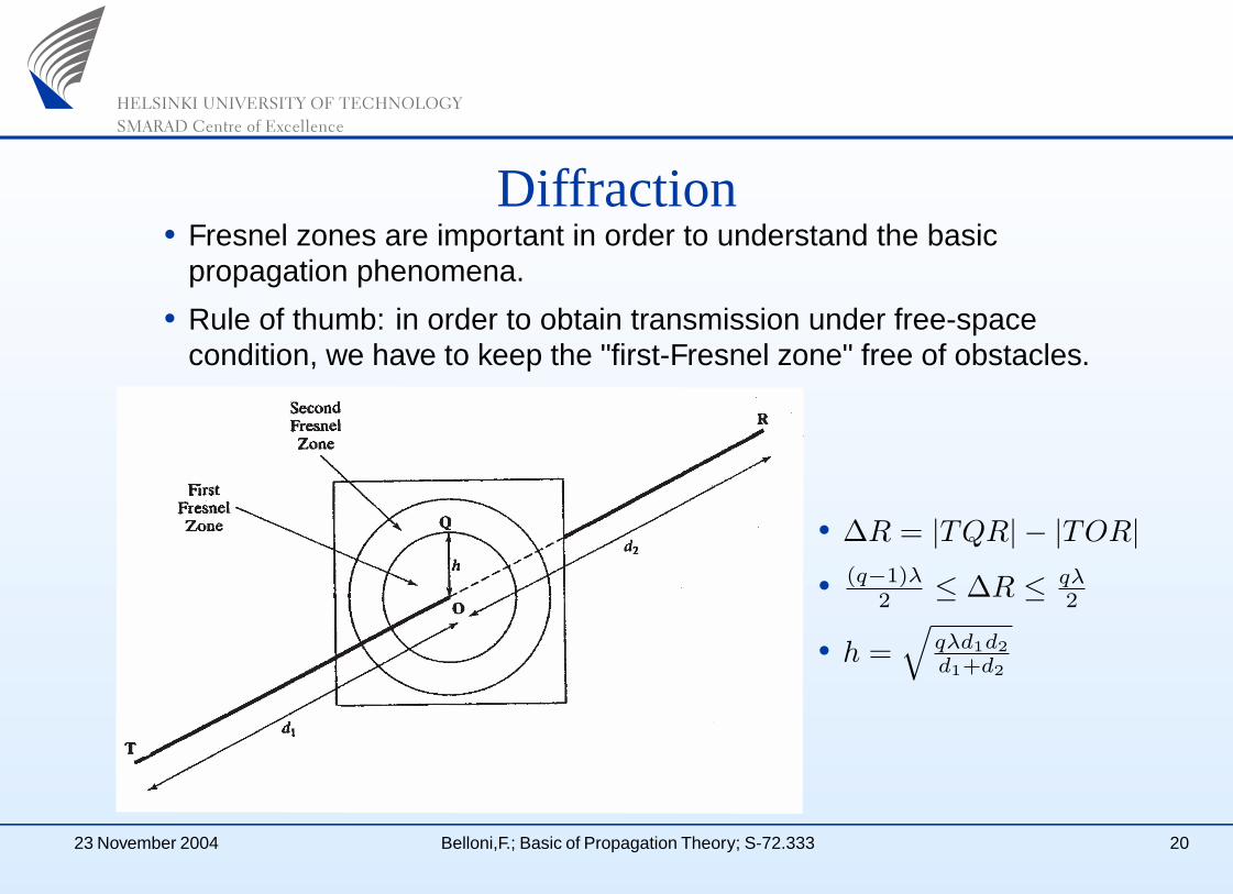
Diffraction• Fresnel zones are important in order to understand the basic

propagation phenomena.• Rule of thumb: in order to obtain transmission under free-space

condition, we have to keep the "first-Fresnel zone" free of obstacles.

• ∆R = |TQR| − |TOR|• (q−1)λ

2 ≤ ∆R ≤ qλ2

• h =√

qλd1d2d1+d2



Diffraction Losses

−3 −2 −1 0 1 2 3

−5

0

5

10

15

20

25

Diffraction parameter (ν)

Pat

h−lo

ss r

elat

ive

to th

e fr

ee−

spac

e (d

B)

• A perfectly absorbing screen is placed between the TX and RX.• When the knife-edge is even with the LOS, the electric field is

reduced by one-half and there is a 6-dB loss in signal power.



Terrestrial Propagation: Statistical Models• By measuring the propagation characteristics in a variety of

environments (urban, suburban, rural), we develop a model basedon the measured statistics for a particular class of environments.

• In general, they are easy to describe but they are not accurate.• The statistical approach is broken down into two components:

- median path loss;- local variations;



Terrestrial Propagation: Statistical Models• Median path loss: investigations motivate a general propagation

model such as PT

PR= β

rn , where r is the distance between TX andRX, n is the path-loss exponent and the parameter β represents aloss that is related to frequency , antenna heights, ...

Environment n

Free-Space 2

Flat Rural 3

Rolling Rural 3.5

Suburban, low rise 4

Dense Urban, Skyscrapers 4.5

• Local variations: the variation about the median can be modelledas a log-normal distribution (shadowing).



Indoor propagation• To study the effects of indoor propagations has gained more and

more importance with the growth of cellular telephone.• Wireless design has to take into account the propagation

characteristics in high-density location.• Wireless Local Area Networks (LAN’s) are being implemented to

eliminate the cost of wiring of rewiring buildings.• Indoor path-loss model

LP (dB) = β(dB) + 10 log10

( r

r0

)n

+P∑

p=1

WAF(p) +Q∑

q=1

FAF(q)

- WAF ⇒ Wall Attenuation Factor- FAF ⇒ Floor attenuation Factor- r ⇒ dinstance TX and RX- r0 ⇒ reference distance (1 m)- Q and P ⇒ number of floors and walls, respectively.



Conclusions• The link budget may be improved by using directional instead of

isotropic antennas.• There is a trade off between the accuracy and the computational

complexity for propagation models.• The polarization of electromagnetic waves is an important issue for

wireless communication.



References• Haykin, S.; Moher, M.; Modern Wireless Communications ISBN

0-13-124697-6, Prentice Hall 2005.• https://ewhdbks.mugu.navy.mil/POLARIZA.HTM• http://www.walter-fendt.de/ph11e/emwave.htm• Paraboni, A.; Antenne, McGraw-Hill 1999.• Saunders, S.; Antennas and Propagation for Wireless

Communication Systems, Wiley, 2000.• Vaughan, R.; Andersen, J.B.; Channels, Propagation and Antennas

for Mobile Communications , IEE, 2003.• Bertoni, H.; Radio Propagation for Modern Wireless Systems,

Prentice Hall, 2000.


https://ewhdbks.mugu.navy.mil/POLARIZA.HTM

http://www.walter-fendt.de/ph11e/emwave.htm


Homeworks• Let us assume a right-hand circular polarization with Ex = 1 and

Ey = −j. Compute the loss in dB in a wireless link when thehorizontal component is attenuated by 6-dB.

• In case of physical models for terrestrial propagation, which are thebasic models of propagation. Explain briefly each of them.


s-72.333 physical layer methods in wireless · pdf file · 2016-01-28basic of...

Documents