rural pipeline flow and water quality st udy final report
TRANSCRIPT

RURAL PIPELINE FLOW AND WATER QUALITY STUDY
FINAL REPORT
by
G. Putz and J.P. Mills
Department of Civil and Geological Engineering
University of Saskatchewan
for the
Saskatchewan Association of Rural Water Pipelines
and
PFRA, Agriculture and Agri-Food Canada
Saskatoon, Saskatchewan
July 2002

Final Report Rural Water Pipeline Study July, 2002
i
TABLE OF CONTENTS
1. BACKGROUND...................................................................................................................... 1 1.1. Introduction................................................................................................................. 1 1.2. Study Objectives ......................................................................................................... 2 1.3. Field Locations............................................................................................................ 2 1.4. Study Period................................................................................................................ 2 1.5. Report Contents .......................................................................................................... 2
2. MONITORING METHODS....................................................................................................... 6 2.1. Hydraulic Measurements ............................................................................................ 6
2.1.1. Flow Monitoring ................................................................................................. 6 2.1.2. Pressure Monitoring............................................................................................ 9
2.2. Water Quality Measurements.................................................................................... 10 2.2.1. Water Temperature ........................................................................................... 11 2.2.2. Turbidity............................................................................................................ 12 2.2.3. Particle Size and Count..................................................................................... 12 2.2.4. Dissolved Organic Carbon................................................................................ 12 2.2.5. Biodegradable Dissolved Organic Carbon........................................................ 12 2.2.6. Epifluorescent Bacterial Counts........................................................................ 12 2.2.7. Chlorine Residual.............................................................................................. 13 2.2.8. Heterotrophic Plate Counts ............................................................................... 13
2.3. Biofilm Measurements.............................................................................................. 13 2.4. Difficulties and Problems ......................................................................................... 16
3. MONITORING RESULTS....................................................................................................... 17 3.1. Hydraulic Data .......................................................................................................... 17
3.1.1. Taylorside/Ethelton........................................................................................... 17 3.1.2. Lucky Lake North ............................................................................................. 22
3.2. Water quality data ..................................................................................................... 26 3.2.1. Taylorside/Ethelton........................................................................................... 26 3.2.2. Coteau Hills ...................................................................................................... 36
3.3. Biofilm Sampling Data ............................................................................................. 44 3.3.1. Taylorside/Ethelton........................................................................................... 44 3.3.2. Coteau Hills ...................................................................................................... 45
4. HYDRAULIC MODELLING ................................................................................................... 46 4.1. Background ............................................................................................................... 46 4.2. Model Construction .................................................................................................. 46
4.2.1. Model Links: ..................................................................................................... 46 4.2.2. Model Nodes:.................................................................................................... 48 4.2.3. User Demand .................................................................................................... 48 4.2.4. Delivery point representation............................................................................ 48 4.2.5. Booster Station Representation......................................................................... 49
4.3. Flow and Pressure Simulation .................................................................................. 50 4.4. Residence Time......................................................................................................... 53

Final Report Rural Water Pipeline Study July, 2002
ii
5. DISCUSSION OF RESULTS.................................................................................................... 56 5.1. Flow and Pressure ..................................................................................................... 56 5.2. Water Quality............................................................................................................ 57 5.3. Biofilm Development................................................................................................ 58
6. RECOMMENDATIONS .......................................................................................................... 58 7. ACKNOWLEDGEMENTS ....................................................................................................... 60 8. REFERENCES ...................................................................................................................... 61
APPENDIX A PHOTOGRAPHS OF MONITORING LOCATIONS............................... 62
APPENDIX B EPANET MODEL AND DATA FILE.......................................................... 66
LIST OF FIGURES
FIGURE 1 TAYLORSIDE/ETHELTON BRANCH PIPELINE, MONITORING AND SAMPLING LOCATIONS. ................................................................................................................................. 3
FIGURE 2 MELFORT REGIONAL WATER TREATMENT PLANT - SOURCE FOR THE SASKWATER
REGIONAL PIPELINE .................................................................................................. 4
FIGURE 3 SASKWATER PUMPHOUSE ON LAKE DIEFENBAKER – SOURCE FOR THE COTEAU HILLS
RURAL WATER PIPELINE.......................................................................................... 4
FIGURE 4 COTEAU HILLS PIPELINE, LUCKY LAKE NORTH BRANCH, MONITORING AND SAMPLING
LOCATIONS............................................................................................................... 5
FIGURE 5 TAYLORSIDE/ETHELTON BRANCH PIPELINE BOOSTER STATION (EXTERIOR).............. 6
FIGURE 6 TAYLORSIDE/ETHELTON BRANCH PIPELINE BOOSTER STATION (INTERIOR)............... 7
FIGURE 7 INSTALLATION OF ULTRASONIC TRANSDUCER FOR FLOW MEASUREMENTS. .............. 7
FIGURE 8 ULTRASONIC FLOW MONITOR DISPLAY DEVICE......................................................... 7
FIGURE 9 COTEAU HILLS PIPELINE BOOSTER STATION #3 (EXTERIOR). .................................... 8
FIGURE 10 COTEAU HILLS PIPELINE BOOSTER STATION #3 (INTERIOR). ..................................... 8
FIGURE 11 TYPICAL FARMSTEAD MONITORING EQUIPMENT. ...................................................... 9
FIGURE 12 TAYLORSIDE/ETHELTON BOOSTER STATION PRESSURE TRANSDUCER..................... 10
FIGURE 13 APPARATUS FOR ON-SITE WATER QUALITY MEASUREMENTS. ................................. 11
FIGURE 14 PIPE EXCAVATION FOR BIOFILM INVESTIGATION. .................................................... 14
FIGURE 15 PIPE SAMPLE PREPARATION FOR BIOFILM INVESTIGATION....................................... 15
FIGURE 16 DAILY AVERAGE FLOW AND PRESSURE RECORDED AT THE TAYLORSIDE/ETHELTON
BOOSTER STATION, JUNE 2000 TO OCTOBER 2001. ................................................ 17
FIGURE 17 EXAMPLE OF HOURLY FLOW AND DISCHARGE PRESSURE DATA RECORDED AUGUST 14 TO 21, 2000 AT THE TAYLORSIDE/ETHELTON BOOSTER STATION. ....... 18
FIGURE 18 EXAMPLE OF HOURLY PRESSURE DATA RECORDED AUGUST 14 TO 21, 2000 AT THE
TAYLORSIDE/ETHELTON BOOSTER STATION, MIDPOINT AND FARPOINT MONITORING
SITES. ..................................................................................................................... 19

Final Report Rural Water Pipeline Study July, 2002
iii
FIGURE 19 EXAMPLE OF HOURLY FLOW AND PRESSURE DATA RECORDED SEPTEMBER 25 TO
OCTOBER 2, 2000 AT THE TAYLORSIDE/ETHELTON MIDPOINT MONITORING SITE... 20
FIGURE 20 EXAMPLE OF HOURLY FLOW AND PRESSURE DATA RECORDED SEPTEMBER 25 TO
OCTOBER 2, 2000 AT THE TAYLORSIDE/ETHELTON FARPOINT MONITORING SITE... 20
FIGURE 21 EXAMPLE OF HOURLY FLOW AND PRESSURE DATA RECORDED AUGUST 7 TO 14, 2001 AT THE TAYLORSIDE/ETHELTON MIDPOINT MONITORING SITE. ............................... 21
FIGURE 22 EXAMPLE OF HOURLY FLOW AND PRESSURE DATA RECORDED AUGUST 7 TO 14, 2001 AT THE TAYLORSIDE/ETHELTON FARPOINT MONITORING SITE. ............................... 21
FIGURE 23 DAILY AVERAGE FLOW AND PRESSURE CALCULATED FOR THE LUCKY LAKE NORTH
BRANCH PIPELINE, MARCH 2000 TO JULY 2001. .................................................... 22
FIGURE 24 PRESSURES ACROSS THE LUCKY LAKE NORTH BRANCH PIPELINE. ......................... 23
FIGURE 25 EXAMPLE OF HOURLY FLOW AND PRESSURE DATA RECORDED SEPTEMBER 17 TO 24, 2000 AT THE LUCKY LAKE NORTH MIDPOINT MONITORING SITE. ........................... 24
FIGURE 26 EXAMPLE OF HOURLY FLOW AND PRESSURE DATA RECORDED SEPTEMBER 17 TO 24, 2000 AT THE LUCKY LAKE NORTH FARPOINT MONITORING SITE. ........................... 25
FIGURE 27 EXAMPLE OF HOURLY FLOW AND PRESSURE DATA RECORDED JUNE 6 TO 13, 2001 AT
THE LUCKY LAKE NORTH FARPOINT MONITORING SITE. ......................................... 25
FIGURE 28 WATER TEMPERATURE MEASURED AT THE TAYLORSIDE/ETHELTON MONITORING SITES. ............................................................................................................................... 26
FIGURE 29 TURBIDITY MEASURED AT THE TAYLORSIDE/ETHELTON MONITORING SITES. ......... 27
FIGURE 30 PARTICLE SIZE DATA (2 TO 5 µM) MEASURED AT TAYLORSIDE/ETHELTON SITES. .. 28
FIGURE 31 PARTICLE SIZE DATA (5 TO 10 µM) MEASURED AT TAYLORSIDE/ETHELTON SITES. 29
FIGURE 32 PARTICLE SIZE DATA (10 TO 15 µM) MEASURED AT TAYLORSIDE/ETHELTON SITES. .. ............................................................................................................................... 29
FIGURE 33 PARTICLE COUNTS AT THE TAYLORSIDE/ETHELTON MIDPOINT SITE. ...................... 30
FIGURE 34 PARTICLE COUNTS AT THE TAYLORSIDE/ETHELTON FARPOINT SITE. ...................... 30
FIGURE 35 DISSOLVED ORGANIC CARBON MEASURED AT THE TAYLORSIDE/ETHELTON MONITORING
SITES. ..................................................................................................................... 31
FIGURE 36 BIODEGRADABLE DISSOLVED ORGANIC CARBON MEASURED AT THE
TAYLORSIDE/ETHELTON MONITORING SITES. ......................................................... 32
FIGURE 37 EPIFLUORESCENT BACTERIA COUNTS MEASURED AT THE TAYLORSIDE/ETHELTON
MONITORING SITES. ................................................................................................ 33
FIGURE 38 TOTAL CHLORINE RESIDUAL MEASURED AT THE TAYLORSIDE/ETHELTON MONITORING
SITES. ..................................................................................................................... 34
FIGURE 39 FREE CHLORINE RESIDUAL MEASURED AT THE TAYLORSIDE/ETHELTON MONITORING
SITES. ..................................................................................................................... 35
FIGURE 40 HPC AND FREE CHLORINE RESIDUAL FROM AUGUST 13, 2001 TO SEPTEMBER 18, 2001 IN THE TAYLORSIDE/ETHELTON PIPELINE. .............................................................. 36
FIGURE 41 WATER TEMPERATURE MEASURED AT LUCKY LAKE NORTH MONITORING SITES.... 37
FIGURE 42 TURBIDITY DATA MEASURED AT LUCKY LAKE NORTH MONITORING SITES. ........... 38

Final Report Rural Water Pipeline Study July, 2002
iv
FIGURE 43 PARTICLE SIZE DATA (2 TO 5 µM) MEASURED AT LUCKY LAKE NORTH SITES. ....... 39
FIGURE 44 PARTICLE SIZE DATA (5 TO 10 µM) MEASURED AT LUCKY LAKE NORTH SITES. ..... 39
FIGURE 45 PARTICLE SIZE DATA (10 TO 15 µM) MEASURED AT LUCKY LAKE NORTH SITES. ... 40
FIGURE 46 PARTICLE COUNTS AT LUCKY LAKE NORTH MIDPOINT SITE. .................................. 40
FIGURE 47 PARTICLE COUNTS AT LUCKY LAKE NORTH FARPOINT SITE. .................................. 41
FIGURE 48 DISSOLVED ORGANIC CARBON MEASURED AT THE LUCKY LAKE NORTH MONITORING
SITES. ..................................................................................................................... 42
FIGURE 49 BIODEGRADABLE DISSOLVED ORGANIC CARBON MEASURED AT THE LUCKY LAKE ... NORTH MONITORING SITES. .................................................................................... 42
FIGURE 50 EPIFLUORESCENT BACTERIA COUNTS MEASURED AT THE LUCKY LAKE NORTH
MONITORING SITES. ................................................................................................ 43
FIGURE 51 PIPE INTERIOR SURFACES EXCAVATED FROM TAYLORSIDE/ETHELTON BRANCH PIPELINE
JELLICOE FARM ON THE LEFT, GROAT FARM ON THE RIGHT. ................................... 44
FIGURE 52 PIPE INTERIOR SURFACES EXCAVATED FROM LUCKY LAKE NORTH BRANCH PIPELINE
TULLIS FARM (MIDPOINT)ON THE LEFT, EREMENKO FARM (FARPOINT) ON THE RIGHT. ............................................................................................................................... 45
FIGURE 53 SCHEMATIC REPRESENTATION OF TAYLORSIDE/ETHELTON PIPELINE WITHIN EPANET ................................................................................................................................... 47
FIGURE 54 TYPICAL USER DELIVERY POINT REPRESENTATION WITHIN EPANET..................... 49
FIGURE 55 TAYLORSIDE/ETHELTON BOOSTER STATION REPRESENTATION WITHIN EPANET .. 50
FIGURE 56 SIMULATION PRESSURE VS. MEASURED AT THE TAYLORSIDE/ETHELTON BOOSTER
STATION. ................................................................................................................ 51
FIGURE 57 SIMULATION FLOW VS. MEASURED AT THE TAYLORSIDE/ETHELTON BOOSTER STATION. ............................................................................................................................... 51
FIGURE 58 PRESSURE AND FLOW SIMULATION VS. MEASURED AT THE MIDPOINT..................... 52
FIGURE 59 PRESSURE AND FLOW SIMULATION VS. MEASURED AT THE FARPOINT..................... 53
FIGURE 60 RESIDENCE TIMES TO VARIOUS POINTS – BASED UPON THE THIRD QUARTER 2000 FLOW
SIMULATION ........................................................................................................... 54
FIGURE 61 A CONTOUR REPRESENTATION OF RESIDENCE TIMES – BASED UPON THE THIRD QUARTER
2000 FLOW SIMULATION ........................................................................................ 55
FIGURE 62 TAYLORSIDE/ETHELTON MIDPOINT MONITORING LOCATION. ................................. 62
FIGURE 63 TAYLORSIDE/ETHELTON MIDPOINT MONITORING SET-UP........................................ 62
FIGURE 64 TAYLORSIDE/ETHELTON FARPOINT MONITORING LOCATION. ................................. 63
FIGURE 65 TAYLORSIDE/ETHELTON FARPOINT MONITORING SET-UP........................................ 63
FIGURE 66 LUCKY LAKE NORTH MIDPOINT MONITORING LOCATION........................................ 64
FIGURE 69 LUCKY LAKE NORTH FARPOINT MONITORING LOCATION........................................ 65
FIGURE 70 LUCKY LAKE FARPOINT MONITORING SET-UP CLOSE-UP......................................... 65

Final Report Rural Water Pipeline Study July, 2002
v
LIST OF TABLES
TABLE 1 TAYLORSIDE/ETHELTON BIOFILM INVESTIGATION RESULTS. ...................................... 44
TABLE 2 LUCKY LAKE NORTH BIOFILM INVESTIGATION RESULTS............................................. 45
TABLE 3 TAYLORSIDE/ETHELTON BOOSTER STATION FLOW CHARACTERISTICS ........................ 56

Final Report Rural Water Pipeline Study July, 2002
1
Rural Pipeline Flow and Water Quality Study
1. Background
1.1. Introduction
Individual family farms and agricultural operations on the Canadian prairies are often forced to rely upon poor quality surface waters for domestic and agricultural needs. Ground water in this region is often highly mineralized, and the yield is frequently insufficient or unreliable. Excessive distances to continuously flowing rivers generally render them uneconomical as a water source for individual users. Therefore, rural water sources on the Canadian prairies are commonly shallow impoundments on local streams or excavated dugouts that collect runoff water from local agricultural land. Consequently, the water collected has high concentration of dissolved organic carbon (DOC causing taste, odour and colour problems), nitrogen and phosphorous (which promote algae growths which further contribute to taste, odour and colour) and high turbidity (Sketchell et al. 1993, Corkal 1997). Dugout and shallow impoundment waters commonly have DOC levels many times higher than major rivers. For example, South Saskatchewan River water has DOC of 2 to 4 mg/L, whereas average dugout DOC is reported to be approximately 13 mg/l (Corkal 1997). Dugouts and reservoirs can also be contaminated with microbial pathogens such as fecal bacteria and/or protozoan cysts (Giardia and Cryptosporidium) originating from the agricultural land.
One strategy for overcoming these problems has been the construction of small diameter, low flow, rural water pipelines from larger regional water treatment facilities or from high quality raw water sources (Pochylko and Morrison, 2000). These rural water pipeline systems distribute water to a group of distributed farmsteads and agricultural operations that organize and finance the construction and operation of the pipeline (Pochylko et al., 2000). Despite the fact these pipelines systems generally provide access to better quality water, there is still potential for water quality problems. These problems can result from biofilm growth in the pipeline system. A review of biofilm effects upon water quality and the factors contributing its development in water distribution pipelines was recently completed (Putz, 2000). The review was based primarily upon investigations conducted on urban systems (or under laboratory conditions simulating urban conditions) because few studies specific to rural water pipeline systems have been published.
The literature review concluded that rural water pipelines may be highly susceptible to biofilm development and associated water quality deterioration problems due to the relatively high levels of DOC in source waters on the prairies, and the long retention times in these systems due to the low flow design and the wide spatial distribution of users. As a result of this concern, and the lack of long-term measurements on the hydraulic characteristics and demand patterns in rural pipelines, a collaborative research program was established between the University of Saskatchewan and Agriculture and Agri-Food Canada with financial support from the Saskatchewan Association of Rural Water Pipelines. Many other agencies, groups and individuals have contributed to the study. Their contributions are acknowledged in Section 7 of this report.
Final Report Rural Water Pipeline Study July, 2002
2
1.2. Study Objectives
The objectives of the rural pipeline flow and water quality study were to: 1) establish monitoring stations on two rural pipeline systems (one treated water pipeline and one untreated water pipeline), 2) collect data at these monitoring sites to characterize typical flow and pressure patterns in the rural pipelines, 3) collect water quality data at the monitoring sites to investigate changes in water quality as water flows through the pipeline, and 4) investigate modelling tools to predict flow, pressure and water quality changes in the rural pipelines using the data collected at the monitoring sites.
1.3. Field Locations
Two rural pipelines were selected to conduct field studies on with the cooperation of the Melfort Rural Pipeline Association and the Coteau Hills Pipeline Association. Each pipeline transports water to a widely distributed group of farmsteads and agricultural enterprises.
The Taylorside/Ethelton system is a branch pipeline receiving treated water from the Melfort Regional Water Treatment Plant (see Figure 1 and Figure 2). The system serves forty two users. A booster station is located close to the take-off point from the regional pipeline. Thirty six users are located downstream the booster station and hence their service pressure is regulated by the booster station pump. The remaining six users’ service pressure is controlled the SaskWater Corporation pumping facilities on the regional pipeline.
The Lucky Lake North system is a branch of the Coteau Hills Pipeline that is a major regional pipeline that carries untreated water from a main pumphouse located on Lake Diefenbaker in a SaskWater facility (see Figure 3 and Figure 4). A series of booster pump stations is located along the regional pipeline to maintain system pressure. The take-off for the Lucky Lake North branch line is located between booster station #3 and #4 (see Figure 4).
1.4. Study Period
Project planning and site selection began in January 2000. Equipment was purchased, and monitoring, sampling and analysis procedures were developed during the period February to May 2000. Installation of field equipment was conducted in late May and early June 2000. Monitoring, sampling and analysis began in mid June 2000. Originally the study was scheduled to continue only until Spring 2001. However, a recommendation was made and approved to continue the monitoring and sampling activities until September 2001 to allow collection of additional long-term data. All sampling and monitoring ended in September 2001 and all equipment removed in October 2001. Sample analysis work continued until January 2002.
1.5. Report Contents
This report contains a summary of activities and data collected during the project. Section 2 describes the monitoring, sampling and analysis procedures utilized during the project. Section 3 presents a summary of the data collected including flow and pressure measurements, water quality analyses and biofilm sampling. Section 4 outlines the computer modelling that has been conducted in conjunction with the project. The data findings are discussed in Section 5 and recommendations presented in Section 6. Acknowledgements and references are listed in Sections 7 and 8.

Final Report Rural Water Pipeline Study July, 2002
3
Figure 1 Taylorside/Ethelton branch pipeline, monitoring and sampling locations.
Jellicoe Farm
Groat Farm

Final Report Rural Water Pipeline Study July, 2002
4
Figure 2 Melfort Regional Water Treatment Plant - source for the SaskWater regional pipeline
Figure 3 SaskWater pumphouse on Lake Diefenbaker – source for the Coteau Hills Rural Water Pipeline

Final Report Rural Water Pipeline Study July, 2002
5
14
1
2
3 4
3 2
1
5 7,6
4
13
12
11
10
8
9
Lucky Lake
Lake
Die
fenb
aker
SW Pumphouse
Far Point
Mid Point
Booster #3
0 2 4Miles
Figure 4 Coteau Hills Pipeline, Lucky Lake North branch, monitoring and sampling locations.

Final Report Rural Water Pipeline Study July, 2002
6
2. Monitoring Methods
2.1. Hydraulic Measurements
Flow and pressure data were continuously collected on each of the pipelines during the period June 2000 to September 2001. On the Taylorside/Ethelton branch pipeline data was collected at two user locations (one near the midpoint of the system and one near the farpoint), and at the booster station pumphouse located near the connection to the SaskWater regional pipeline (see Figure 1). In addition, flow records for the all the other branch pipelines supplied from the regional pipeline were obtained from SaskWater Corporation. Similarly, on the Lucky Lake North branch pipeline data was collected at two user locations (one near the midpoint of the system and one near the farpoint) and at booster stations #3 and #4 upstream and downstream of the branch take-off point (see Figure 4). Flow records from the main pumphouse on Lake Diefenbaker were obtained from SaskWater Corporation.
2.1.1. Flow Monitoring
2.1.1.1. Booster Station (System) Flows
Taylorside/Ethelton
The booster station on Taylorside/Ethelton pipeline (see Figure 5 and Figure 6) was not originally equipped to record flow. Therefore, the booster station was retrofitted with a temporary, non-intrusive, ultrasonic flow measurement device. The ultrasonic transducer was attached to the station discharge line (see Figure 7). The transducer produced a continuous electronic signal proportional to the system flow. This signal was feed to a display device and a datalogger located in the booster station shed (see Figure 8). The station flow was continuously displayed, but time-averaged over 5 minute intervals before being recorded on the datalogger.
Figure 5 Taylorside/Ethelton branch pipeline booster station (exterior).

Final Report Rural Water Pipeline Study July, 2002
7
Figure 6 Taylorside/Ethelton branch pipeline booster station (interior).
Figure 7 Installation of ultrasonic transducer for flow measurements.
Figure 8 Ultrasonic flow monitor display device.
Final Report Rural Water Pipeline Study July, 2002
8
Lucky Lake North
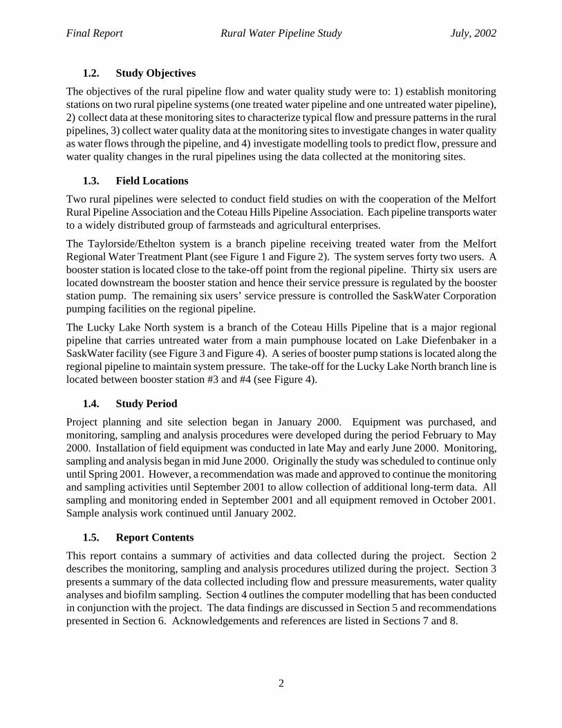
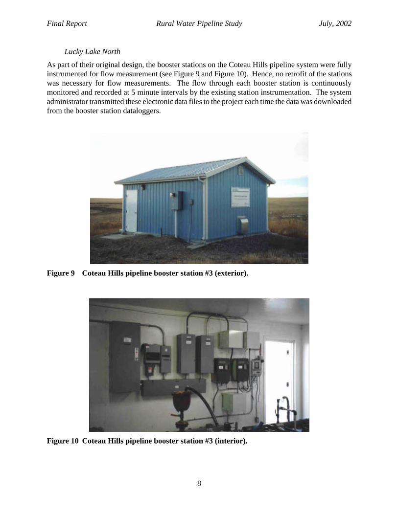
As part of their original design, the booster stations on the Coteau Hills pipeline system were fully instrumented for flow measurement (see Figure 9 and Figure 10). Hence, no retrofit of the stations was necessary for flow measurements. The flow through each booster station is continuously monitored and recorded at 5 minute intervals by the existing station instrumentation. The system administrator transmitted these electronic data files to the project each time the data was downloaded from the booster station dataloggers.
Figure 9 Coteau Hills pipeline booster station #3 (exterior).
Figure 10 Coteau Hills pipeline booster station #3 (interior).

Final Report Rural Water Pipeline Study July, 2002
9
2.1.1.2. Farmstead Flows
At each of the farmstead monitoring locations a high-resolution electronic pulse water meter was installed. The high-resolution water meter has a large pulse to volume ratio that allows accurate measurement of short duration flows. The datalogger was located in the user’s basement and continuously recorded the number of pulses produced by the water meter during successive 5-minute intervals. This data was downloaded periodically. A conversion factor was then applied to the pulse count to produce a continuous record of the rate of water use by each farmstead. A typical water meter and datalogger installation is shown in Figure 11. Photographs of each farmstead monitoring station are presented in Appendix A.
Figure 11 Typical farmstead monitoring equipment.
2.1.2. Pressure Monitoring
2.1.2.1. Booster Station Inset and Discharge Pressures
Taylorside/Ethelton
The original pressure measurement instrumentation installed at the Taylorside/Ethelton pipeline booster station consisted of analog gauges located on the inlet and discharge line of the booster pump. Therefore, in order to continuously monitor and record the station inlet and outlet pressures the station was retrofitted with electronic pressure transducers. The pressure transducers were tapped into the same locations as the existing analog gauges (see Figure 12). The datalogger that was installed to record the flow data was also used to record the signal from each pressure transducer. The station inlet and outlet pressures were continuously monitored and time-averaged over 5-minute intervals before being recorded on the datalogger.

Final Report Rural Water Pipeline Study July, 2002
10
Figure 12 Taylorside/Ethelton booster station pressure transducer.
Lucky Lake North
The booster stations on the Coteau Hills pipeline system were fully instrumented for pressure measurements as part of their original design. Hence, no retrofit of the stations was necessary for pressure measurement. The inlet and outlet pressure at each booster station is continuously monitored and recorded at 5 minute intervals by the existing station instrumentation. The system administrator transmitted these electronic data files to the project each time the data was downloaded from the booster station dataloggers.
2.1.2.2. System Pressure at Farmstead Locations
At each of the four farmstead monitoring locations an electronic pressure transducer was installed upstream of the delivery point pressure reducer and/or flow restrictor value. The datalogger installed to record the user flow was also used to record time-averaged system pressure over 5-minute intervals. This data was downloaded periodically and used to produce a continuous record of system pressure available at the farmstead service connection during cistern filling and shut-off periods. An example pressure transducer and datalogger installation is shown in Figure 11. Photographs of each farmstead monitoring station are presented in Appendix A.
2.2. Water Quality Measurements
In conjunction with the hydraulic measurements, a water quality sampling and analysis program was conducted to measure water quality at each user monitoring locations, the booster station at the head of each pipeline, and at the pipeline source. The pipeline source for the Taylorside/Ethelton branch is water leaving the Melfort Regional Water Treatment Plant. The pipeline source for the Lucky Lake North branch is the Coteau Hills Pipeline pumping facility located in the SaskWater pumphouse on Lake Diefenbaker.
The water quality sampling and analysis program measured temperature, turbidity, particle size and count, dissolved organic carbon (DOC), biodegradable dissolved organic carbon (BDOC) and epifluorescent bacterial counts on the Taylorside/Ethelton branch (treated water) and Lucky Lake North branch (untreated water) pipelines. Free and combined chlorine residual concentrations were also measured on the treated water pipeline. Heterotrophic plate counts were also conducted on samples taken from the treated water pipeline over a one month period near the end of the study.
Final Report Rural Water Pipeline Study July, 2002
11
Water quality sampling was conducted at each site at one to three week intervals during the summer and fall months of 2000, and during the summer of 2001, depending on the observed water temperature in the pipeline. Peak water temperatures were expected to produce peak biological activity and hence the greatest potential for water quality deterioration. Therefore, sampling frequency was increased during the summer and early fall. Over the winter period the frequency of sampling was reduced to approximately four-week intervals.
The Taylorside/Ethelton and Lucky Lake North branch pipeline monitoring sites were sampled a total of 24 and 23 times, respectively. In total 752 DOC measurements were taken resulting in 376 DOC readings and 376 BDOC readings, 188 particle size counts, 188 turbidity measurements, 200 epifluorescent bacterial counts, 96 chlorine residual measurements, and 32 heterotrophic plate counts were completed. In addition, 188 water temperature measurements were recorded during site visits. A total of 24 heterotrophic plate count samples were collected from the Taylorside/Ethelton branch from August 13, 2001 to September 18, 2001 (during the estimated peak activity period).
2.2.1. Water Temperature
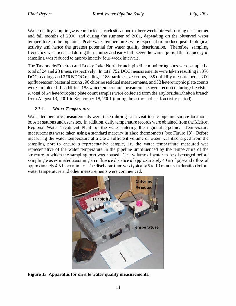
Water temperature measurements were taken during each visit to the pipeline source locations, booster stations and user sites. In addition, daily temperature records were obtained from the Melfort Regional Water Treatment Plant for the water entering the regional pipeline. Temperature measurements were taken using a standard mercury in glass thermometer (see Figure 13). Before measuring the water temperature at a site a sufficient volume of water was discharged from the sampling port to ensure a representative sample, i.e. the water temperature measured was representative of the water temperature in the pipeline uninfluenced by the temperature of the structure in which the sampling port was housed. The volume of water to be discharged before sampling was estimated assuming an influence distance of approximately 40 m of pipe and a flow of approximately 4.5 L per minute. The discharge time was typically 5 to 10 minutes in duration before water temperature and other measurements were commenced.
Turbidity
ChlorineResidual
Temperature
Figure 13 Apparatus for on-site water quality measurements.

Final Report Rural Water Pipeline Study July, 2002
12
2.2.2. Turbidity
Turbidity measurements were taken during visits to each monitoring site. These measurements were taken with a Hach portable turbidimeter (see Figure 13). In addition, on-line Great Lakes Instruments turbidimeters were installed at the two user monitoring sites on the Taylorside/Ethelton branch pipeline. The on-line turbidimeters provided a continuous electronic signal proportional to turbidity during cistern filling to the dataloggers at these two user sites.
2.2.3. Particle Size and Count
Water samples for particle counting were taken during visits to each monitoring site. The samples were transported to the Department of Civil Engineering, Environmental Engineering Laboratory for analysis. Analysis was conducted with a MetOne WGS267 particle counter. The instrument provides particle count results in six size ranges (2-5, 5-10, 10-15, 15-20, 20-40, >40 µm). Particle counting results are unavailable for samples during the period (October to December, 2000). During this time the instrument was fouled while analysing highly turbid samples from another research project. As a result, the instrument had to be sent to the manufacturer for recalibration.
2.2.4. Dissolved Organic Carbon
Water samples for dissolved organic carbon (DOC) analysis were taken during visits to each monitoring site. The samples were collected in acid washed bottles and transported to the Department of Civil Engineering, Environmental Engineering Laboratory for initial preparation. At the Environmental Engineering laboratory the samples were filtered and transferred to smaller sample bottles for shipment to the Environment Canada Laboratory at the National Water Research Institute in Saskatoon. At the Environment Canada laboratory the samples were analysed using a Tekmar Dohrmann, UV-persulphate dissolved organic carbon analyser.
DOC samples were placed in cooler chests packed with ice during transport to suppress biological activity. Similarly, samples were stored in refrigerators at 4 ºC before pre-treatment and analysis. Studies conducted by the Environment Canada have demonstrated that samples handled and stored observing these conditions maintain sample integrity for several months. Samples were frequently stored for several weeks before analyses commenced.
2.2.5. Biodegradable Dissolved Organic Carbon
The biodegradable dissolved organic carbon (BDOC) content of water samples that were collected at each monitoring site was determined using the procedure described by Servais et al., 1989. The initial DOC of the samples was determined as described above. A portion of same water sample was filter sterilized using a 0.2 µm polycarbonate filter, then inoculated with natural river water microbes and incubated for 28 days. Following incubation the DOC of the sample was measured. The BDOC was determined by taking the difference between the initial and final DOC measurements and then correcting for blank measurements of the DOC content of the river water inoculum.
2.2.6. Epifluorescent Bacterial Counts
Water samples for epifluorescent bacterial counts (EBC) were taken during visits to each monitoring site. The EBC counts were determined using a modified Standard Methods procedure (9216 B). The modifications to the procedure were based upon the analysis method outlined by Porter and Feig,

Final Report Rural Water Pipeline Study July, 2002
13
1980. The samples were collected in acid washed bottles and transported to the Department of Civil Engineering, Environmental Engineering Laboratory for initial preparation. At the Environmental Engineering laboratory a portion of the water samples were transferred to smaller bottles and treated with fluorescent stain. These samples were stored at the Environmental Engineering Laboratory and periodically taken to Environment Canada at the National Water Research Institute in Saskatoon.. Environment Canada allowed project personnel access to a UV microscope required for EBC analysis. Once at Environment Canada, the project personnel filtered the samples through 0.2 µm polycarbonate filters and counted the bacteria retained on the filters using the UV microscope.
As for the DOC samples, all EBC samples were placed in cooler chests packed with ice during transport to suppress biological activity. Similarly, samples were stored in refrigerators at 4 ºC before pre-treatment and analysis.
Epifluorescent counts do not discern between live and dead cells, therefore they are a measure of the total number of bacterial cells in the water distribution system without regard to viability. With increased turbidity, counting of the epifluorescent bacteria cells becomes increasingly difficult as small particulate matter can be mistaken for bacterial cells. As a result many of the epifluorescent counts were double counted as a check of the results.
2.2.7. Chlorine Residual
Chlorine residual measurements were taken during each visit to the pipeline source, booster station pumphouse and the user sites on the Taylorside/Ethelton system. In addition, chlorine residual records were obtained from the Melfort Regional Water Treatment Plant for the water entering the regional pipeline. No chlorine residual measurements were taken on the Lucky Lake branch pipeline because it carries untreated water.
The chlorine residual measurements were conducted using the standard DPD titrimetric procedure using ferrous ammonium sulphate titrant. The procedure allows the determination of both free and combined chlorine residual. The titrations were performed on-site utilizing a portable titration apparatus (see Figure 13).
2.2.8. Heterotrophic Plate Counts
During the last month of sampling program on the Taylorside/Ethelton branch pipeline water samples were collected for heterotrophic plate count (HPC) analysis. Saskatchewan Health provided sample bottles, instructions and analytical services for the HPC analysis. Samples were collected from the pipeline source, the booster station and from the two user locations being monitored. The samples were transported in coolers packed with ice to Saskatoon and then immediately shipped by bus to the Provincial Laboratory in Regina for analysis.
2.3. Biofilm Measurements
In August 2001 excavations were conducted on the two pipelines to remove several sections of pipe. The objective was to investigate the presence of biofilm development on the interior of the in-service high density polyethylene (HDPE) pipe. Two locations for excavation and pipe extraction were selected on each of the branch pipeline systems being studied.
On the Taylorside/Ethelton (treated water) pipeline two locations were selected with large residence times in comparison to other locations on the system. It was expected that the highest potential for

Final Report Rural Water Pipeline Study July, 2002
14
reduced chlorine residual would occur at locations with the largest residence times. Excavations and extractions were conducted on the service connections to the Jellicoe and Groat farm locations (see Figure 1). The Groat farm is located at one of the furthest distances from the branch take-off point. The Jellicoe farm is located near the middle of the branch, however, the water use there is relatively small and the service connection is very long, therefore, the retention time is expected to be large.
On the Lucky Lake North (untreated water) pipeline chlorine residual was not an issue. Therefore, the excavations and extraction were conducted on the service connections at the two user monitoring sites (i.e. midpoint(#10) and farpoint (#14), see Figure 4).
The excavation and extraction procedure consisted of:
i) Locating the pipe trench,
ii) Excavating carefully with a backhoe to near the pipe surface (see Figure 14),
iii) Hand excavation of the material surrounding the pipe for approximately a 3 m length,
iv) Isolating approximately a 1.5 m section of the pipe with pipe squeezers to shut off the flow,
v) Removing approximately a 1m section of pipe,
vi) Cleaning the cut pipe ends and hot fusion welding a replacement section into place,
vii) Slowly releasing the pipe squeezers and testing the fusion welds for leaks, and
viii)Filling the trench will excavated material and smoothing the surface to original grade
Figure 14 Pipe excavation for biofilm investigation.

Final Report Rural Water Pipeline Study July, 2002
15
The exterior of the section of pipe removed from the service connection was thoroughly cleaned and disinfected (see Figure 15 upper and lower left). Then approximately 200 mm lengths were cut from the middle portion of the removed section (see Figure 15 upper right). These short sections were placed in sterile wide mouth sample bottles and filled with sterile distilled water (see Figure 15 lower right). The sample bottles were placed in a cooler chest packed with ice and transported to the Department of Civil Engineering Environmental Engineering laboratory.
Figure 15 Pipe sample preparation for biofilm investigation.
In the laboratory the small pipe section and volume of water in which it was contained was subjected to cleaning by sonic vibration. This procedure removed any biofilm materials attached to the interior surface of the pipe. The volume of water containing the captured material from the pipe interior surfaces was then analysed for heterotrophic bacteria and epifluorescent bacteria count. The count per volume was then related back to the interior surface area of the pipe sample (i.e. count per surface area). The interior surface area was calculated based upon sample length and inside diameter measurements. Samples of the extracted material were also sent to a commercial microbiological laboratory for identification of the dominant bacterial species present.

Final Report Rural Water Pipeline Study July, 2002
16
2.4. Difficulties and Problems
Difficulties and problems were encountered during the data collection program. The majority of these were minor problems with equipment and water quality analysis procedures. Most of these problems were quickly resolved with minimal loss of data. However, several more serious problems arose that could not be resolved. These problems are outlined below:
BDOC analysis on water samples taken in fall 2000 produced values and patterns that were unexpected. The problem was found to be the distilled water source in the Department of Civil Engineering, Environmental Engineering Laboratory. The distillation system there did not reliably remove the DOC from the water used to prepare blank samples used to determine the BDOC contribution of the inoculum. Therefore, the correction for the blanks is subject to increased error and variability. The problem was partially resolved by obtaining ultra-pure distilled water from the Environment Canada laboratory for preparing the blanks. However, the BDOC analyses results beyond fall 2000 continued to more variable than would have been expected and frequently gave negative results.
Problems were encountered in obtaining complete flow records for booster stations #3 and #4 from the Coteau Hills Pipeline Association. Unfortunately, the Association suffered several datalogger malfunctions that left gaps in the continuous flow and pressure data at the booster stations. Further, there is a time synchronization problem between the dataloggers located in the booster stations. Efforts were made by the Association to resolve this problem by adjusting the equipment but were unsuccessful. Project personnel tried to synchronize the data by matching recorded peaks but this proved unreliable. As a result, only the average daily flow for the Lucky Lake North pipeline is considered reliable.
A large amount of sediment had accumulated in the service connection to the midpoint monitoring station on the Lucky Lake North branch pipeline. This caused some problems with taking representative water quality samples. However, its major effect was not discovered until the field program was completed. In the spring of 2001 sediments caused the pulse water meter at the midpoint monitoring station to stop functioning correctly. Flow data was being recorded but unfortunately it was inaccurate. Therefore, no flow data was obtained at this location for the spring and summer of 2001. The pressure readings recorded during this period were not affected.
The particle analyser equipment in the Environmental Engineering laboratory became fouled during the study period (late fall 2000). As result, the analyser had to be sent away for recalibration. Several months of particle count data were lost while the equipment was away and all samples analysed prior to recalibration may not be reliable.
Final Report Rural Water Pipeline Study July, 2002
17
3. Monitoring Results
Summary and example plots of data collected during the period June 2000 to September 2001 are presented in this section.
3.1. Hydraulic Data
3.1.1. Taylorside/Ethelton
Time-averaged flow and pressure data were collected at three monitoring sites on the Taylorside/Ethelton pipeline (the booster pump station near the connection to the SaskWater pipeline, a point near the middle of the branch, and a point at the far extent of the branch). Flow and pressure readings at the booster station were time-averaged over 5 minute intervals before they were recorded on the datalogger. At the middle and far point locations the flow and pressure readings were also time-averaged over 5 minute intervals before they were recorded on the datalogger.
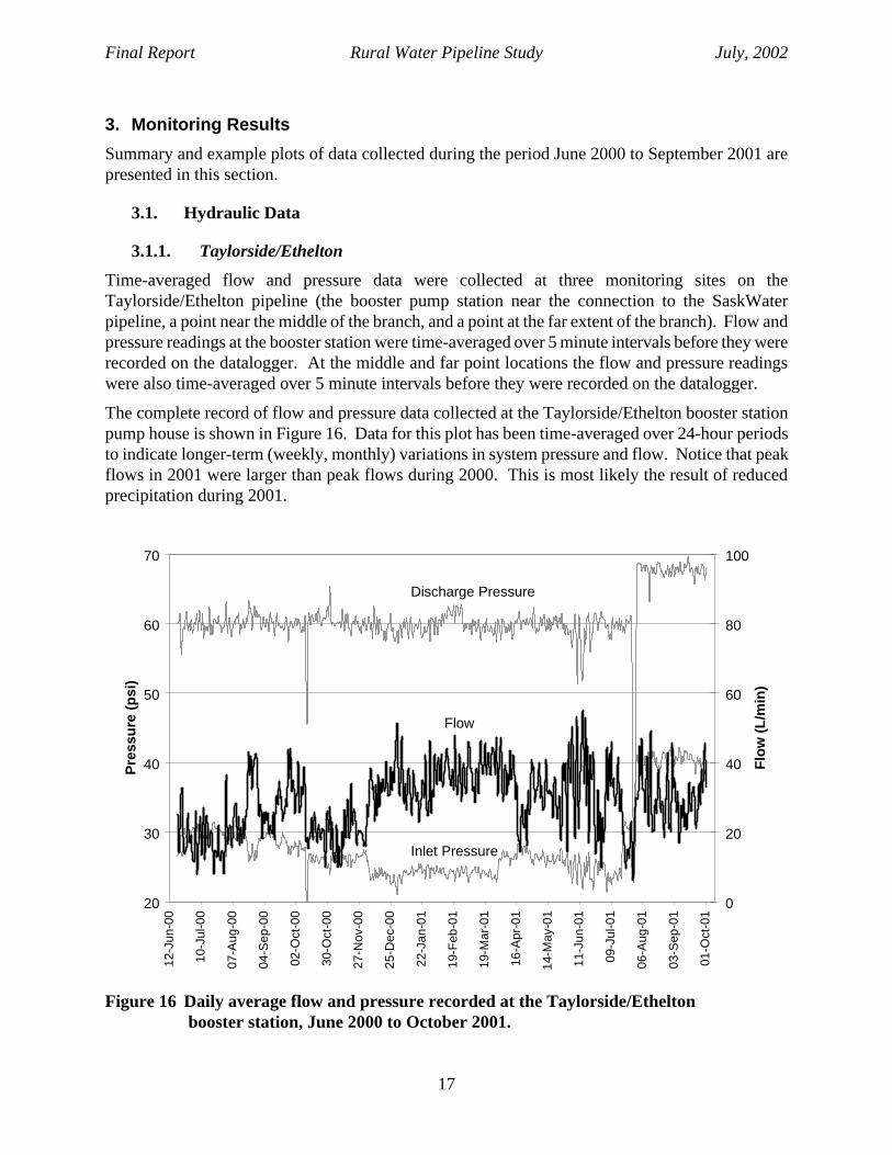
The complete record of flow and pressure data collected at the Taylorside/Ethelton booster station pump house is shown in Figure 16. Data for this plot has been time-averaged over 24-hour periods to indicate longer-term (weekly, monthly) variations in system pressure and flow. Notice that peak flows in 2001 were larger than peak flows during 2000. This is most likely the result of reduced precipitation during 2001.
20
30
40
50
60
70
12-J
un-0
0
10-J
ul-0
0
07-A
ug-0
0
04-S
ep-0
0
02-O
ct-0
0
30-O
ct-0
0
27-N
ov-0
0
25-D
ec-0
0
22-J
an-0
1
19-F
eb-0
1
19-M
ar-0
1
16-A
pr-0
1
14-M
ay-0
1
11-J
un-0
1
09-J
ul-0
1
06-A
ug-0
1
03-S
ep-0
1
01-O
ct-0
1
Pre
ssu
re (
psi
)
0
20
40
60
80
100
Flo
w (
L/m
in)
Discharge Pressure
Flow
Inlet Pressure
Figure 16 Daily average flow and pressure recorded at the Taylorside/Ethelton booster station, June 2000 to October 2001.

Final Report Rural Water Pipeline Study July, 2002
18
Figure 17 shows typical short-term flow and pressure variations at the Taylorside\Ethelton booster station over a one-week period in August 2000. Here the data has been time-averaged over one-hour intervals; hence the plot shows average hourly pressures and flows. The typical daily flow patterns are clearly illustrated in the plot. System flow drops to nearly zero after midnight each night, and generally two peaks flows occur each day, one in the morning and the other in the evening.
0
10
20
30
40
50
60
70
14-Aug-00 15-Aug-00 16-Aug-00 17-Aug-00 18-Aug-00 19-Aug-00 20-Aug-00 21-Aug-00
Pre
ssu
re (
psi
)
0
20
40
60
80
100
120
140
Flo
w (
L/m
in)
Booster Flow
Booster Discharge Pressure
Figure 17 Example of hourly flow and discharge pressure data recorded August 14 to 21, 2000 at the Taylorside/Ethelton booster station.
Typical variations in system pressure at the booster station, midpoint and farpoint monitoring locations during August 14 to 21, 2000 are shown in Figure 18. Average hourly pressures are shown in the plot. Note the booster station discharge pressure is approximately 60 ± 5 psi. At the midpoint the system pressure has only dropped to approximately 55 ± 5 psi. However, at the farpoint the pressure has been reduced to approximately 35 ± 10 psi. The large change in pressure from the midpoint to the farpoint is likely due to increased friction losses that occur through the smaller pipe diameters used toward the periphery of the system.

Final Report Rural Water Pipeline Study July, 2002
19
20
30
40
50
60
70
14-Aug-00 15-Aug-00 16-Aug-00 17-Aug-00 18-Aug-00 19-Aug-00 20-Aug-00 21-Aug-00
Pre
ssu
re (
psi
)
Farpoint Pressure
Booster Discharge Pressure
Midpoint Pressure
Figure 18 Example of hourly pressure data recorded August 14 to 21, 2000 at the Taylorside/Ethelton booster station, midpoint and farpoint monitoring sites.
Figure 19 and Figure 20 show an example of typical flow and pressure variations which occur at the mid and farpoint monitoring sites on the Taylorside/Ethelton system. The week of September 25 to October 2, 2000 (peak weekly system flow for the year 2000) is shown. The data plotted have been time-averaged over one-hour periods. The plots illustrate typical daily flow and pressure patterns. Note the users’ cistern float switch and solenoid valve activations are clearly evident in Figure 19 and Figure 20. Similar plots are shown in Figure 21 and Figure 22 during the period August 7 to 14, 2001 (peak weekly system flow period for the year 2001).
The pressures patterns shown in Figure 19 and Figure 20 at the mid and farpoint monitoring locations are very similar. The difference is approximately a 20 psi translation in pressure magnitude due to elevation, and friction losses occurring between the two monitoring points caused by user demands. The pressure patterns shown in Figure 21 and Figure 22 are also very similar but there is more indication of local influence and significant friction losses in the vicinity of the farpoint site.
Due to dry weather conditions during August 2001 the farpoint farmstead was supplying water for livestock as well as for domestic use. This increased flow requirement is clearly indicated by the increased number of solenoid activations (approx. 12 per week) compared to the previous year (approx. 4 per week). There is also a huge pressure drop evident on August 12, 2001 on Figure 21 and Figure 22. This loss in pressure is most likely the result of flushing operations on the Taylorside/Ethelton system or possibly on the SaskWater regional pipeline.

Final Report Rural Water Pipeline Study July, 2002
20
0
20
40
60
80
25-Sep-00 26-Sep-00 27-Sep-00 28-Sep-00 29-Sep-00 30-Sep-00 1-Oct-00 2-Oct-00
Pre
ssu
re (
psi
)
0
10
20
30
40
Flo
w (
L/m
in)
Figure 19 Example of hourly flow and pressure data recorded September 25 to
October 2, 2000 at the Taylorside/Ethelton midpoint monitoring site.
0
20
40
60
80
25-Sep-00 26-Sep-00 27-Sep-00 28-Sep-00 29-Sep-00 30-Sep-00 1-Oct-00 2-Oct-00
Pre
ssu
re (
psi
)
0
10
20
30
40
Flo
w (
L/m
in)
Pressure
Flow
Figure 20 Example of hourly flow and pressure data recorded September 25 to October 2, 2000 at the Taylorside/Ethelton farpoint monitoring site.

Final Report Rural Water Pipeline Study July, 2002
21
0
20
40
60
80
7-Aug-01 8-Aug-01 9-Aug-01 10-Aug-01 11-Aug-01 12-Aug-01 13-Aug-01 14-Aug-01
Pre
ssu
re (
psi
)
0
10
20
30
40
Flo
w (
L/m
in)
Pressure
Flow
Figure 21 Example of hourly flow and pressure data recorded August 7 to 14, 2001 at the Taylorside/Ethelton midpoint monitoring site.
0
20
40
60
80
7-Aug-01 8-Aug-01 9-Aug-01 10-Aug-01 11-Aug-01 12-Aug-01 13-Aug-01 14-Aug-01
Pre
ssu
re (
psi
)
0
10
20
30
40
Flo
w (
L/m
in)
Pressure
Flow
Figure 22 Example of hourly flow and pressure data recorded August 7 to 14, 2001 at the Taylorside/Ethelton farpoint monitoring site.

Final Report Rural Water Pipeline Study July, 2002
22
3.1.2. Lucky Lake North
Time-averaged flow and pressure data were collected at two monitoring sites on the Lucky Lake North branch pipeline (at a point near the middle of the branch, and at a point at the end of the branch). These flow and pressure readings were time-averaged over 5 minute intervals before they were recorded on the datalogger located in the user’s basement.
Flow and pressure data was also collected by the Coteau Hills pipeline association at booster station #3 and #4 (see Figure 4) using instrumentation incorporated into their pumphouse design (see Figure 10). These electronic flow and pressure readings were manually compiled and sent to the study project on a monthly to bimonthly basis by the Coteau Hills pipeline system operator. Flow and pressure data from the main pumphouse located on Lake Diefenbaker were collected by SaskWater Corporation. These recordings on standard circular chart paper were made available to the project.
Estimated flows and pressures at the Lucky Lake North branch take-off location on the Coteau Hills pipeline are shown in Figure 23. The flow and pressure data were synthesized using data provided by the Coteau Hills Pipeline Association for booster stations #3 and #4. The flow entering the Lucky Lake North branch is the difference in flow between booster stations #3 and #4. The pressure at the take-off point was estimated by conducting total energy calculations accounting for headlosses and elevation between booster station #3 and #4.
40
45
50
55
60
65
70
75
80
Mar
-00
Apr
-00
May
-00
Jun-
00
Jul-0
0
Aug
-00
Sep
-00
Oct
-00
Nov
-00
Nov
-00
Dec
-00
Jan-
01
Feb
-01
Mar
-01
Apr
-01
May
-01
Jun-
01
Pre
ssu
re (
psi
)
0
20
40
60
80
100
120
140
160
Flo
w (
L/m
in)
Pressure
Flow
Figure 23 Daily average flow and pressure calculated for the Lucky Lake North branch pipeline, March 2000 to July 2001.

Final Report Rural Water Pipeline Study July, 2002
23
Figure 23 was prepared using daily average flows and pressures. It was not possible to prepare plots using hourly averages (similar to those shown for Taylorside/Ethelton) due to the time synchronization problems between booster stations described earlier. Also note that several periods of record were lost due to malfunctioning of the recording equipment at the booster stations. Despite these problems, Figure 23 illustrates typical weekly and monthly variations in system pressure and flow that occur in the Lucky Lake North branch.
Figure 24 illustrates pressure variation in the system along the Lucky Lake North branch from booster station #3 (close to the take-off location) to the far point. The data plotted are time-averaged pressures over 15 minute intervals during the week of March 8 to 15, 2001. Note the midpoint pressure is very large in comparison to booster station #3 (120 to 140 psi compared to 60 to 80 psi) because the midpoint is located at a substantially lower elevation. In contrast, the farpoint monitoring station is located on a significant rise of land. As a result the pressure at the farpoint is much lower (approximately 50 to 70 psi during periods of no flow). The pressure at the farpoint drops to approximately 30 psi during flow activations. The flow activations at the farpoint appear to have a strong influence on overall system pressure (note the drops in booster station and midpoint pressures corresponding to the farpoint pressure lows during activations).
0
20
40
60
80
100
120
140
160
8-Mar-01 9-Mar-01 10-Mar-01 11-Mar-01 12-Mar-01 13-Mar-01 14-Mar-01 15-Mar-01
Pre
ssu
re (
psi
)
Booster #3
Farpoint
Midpoint
Figure 24 Pressures across the Lucky Lake North branch pipeline.
Figure 25 and Figure 26 show an example of typical flow and pressure variations which occur at the mid and farpoint monitoring sites on the Lucky Lake North branch. The week of September 17 to 24, 2000 (peak weekly system flow for the year 2000) is shown. The data plotted have been time averaged over one-hour periods. The plots illustrate typical daily flow and pressure patterns. The user cistern float switch and valve activations are less evident in the pressure plot of the midpoint

Final Report Rural Water Pipeline Study July, 2002
24
station compared to the farpoint. At both locations the flow activations are generally a series of grouped short duration flows rather than sustained longer duration flows.
The pressures patterns shown in Figure 25 and Figure 26 at the mid and farpoint monitoring locations are very similar. The difference is a translation in pressure magnitude due to elevation, and friction losses occurring between the two monitoring points caused by user demands. The pressure pattern at the farpoint has much larger differences between the pressure peaks and lows compared to the midpoint, and appears to be strongly influenced by the farpoint flow activations.
A plot of pressure and flow for the farpoint station is also shown in Figure 27 for the period June 6 to 13, 2001 (peak weekly system flow period for the year 2001). The corresponding plot for the midpoint during this period is unavailable due to the flow meter malfunction described earlier. Figure 27 shows the occurrence of two sustained flows at the farpoint. This is likely an example of water demand to fill tanks or vessels other than the users standard cistern. As mentioned early when discussing the Taylorside/Ethelton system, the spring and summer of 2001 were very dry. Therefore, since the farpoint on the Lucky Lake North branch is a cattle operation, the sustained flows may be the result of cattle watering operations.
0
20
40
60
80
100
120
140
160
17-Sep-00 18-Sep-00 19-Sep-00 20-Sep-00 21-Sep-00 22-Sep-00 23-Sep-00 24-Sep-00
Pre
ssu
re (
psi
)
0
1
2
3
4
5
6
7
8
Flo
w (
L/m
in)
Pressure
Flow
Figure 25 Example of hourly flow and pressure data recorded September 17 to 24, 2000 at the Lucky Lake North midpoint monitoring site.

Final Report Rural Water Pipeline Study July, 2002
25
0
10
20
30
40
50
60
70
80
17-Sep-00 18-Sep-00 19-Sep-00 20-Sep-00 21-Sep-00 22-Sep-00 23-Sep-00 24-Sep-00
Pre
ssu
re (
psi
)
0
2
4
6
8
10
12
14
16
Flo
w (
L/m
in)
Pressure
Flow
Figure 26 Example of hourly flow and pressure data recorded September 17 to 24, 2000 at the Lucky Lake North farpoint monitoring site.
0
10
20
30
40
50
60
70
80
6-Jun-01 7-Jun-01 8-Jun-01 9-Jun-01 10-Jun-01 11-Jun-01 12-Jun-01 13-Jun-01
Pre
ssu
re (
psi
)
0
2
4
6
8
10
12
14
16
Flo
w (
L/m
in)
Pressure
Flow
Flow
Pres.
Figure 27 Example of hourly flow and pressure data recorded June 6 to 13, 2001 at the Lucky Lake North farpoint monitoring site.

Final Report Rural Water Pipeline Study July, 2002
26
3.2. Water quality data
Plots of the water quality data collected from June 2000 to September 2001 on each pipeline are presented in this section.
3.2.1. Taylorside/Ethelton
3.2.1.1. Water Temperature
The seasonal change in water temperature and variation between sampling points along the pipeline are shown in Figure 28. The water temperature falls to a minimum in late April and peaks in late August/early September. The seasonal variation is most prominent at the water treatment plant, which receives its source water via a pipeline from Saskatchewan River to the plant’s main reservoir. The difference between the water temperature at the treatment plant and along the rest of the line shows the cooling effect of the ground temperature on the water in the distribution system. The cooling effect is further illustrated by considering the elevated temperature at the water treatment plant in 2001 in comparison to 2000, yet the pipeline temperature remains relatively consistent with that in 2000. The ground temperature significantly influences the temperature of the water in the line due to the long residence times associated with a low flow pipeline and the resulting heat exchange.
Note that the water temperature in the pipeline remains relatively cold for much of the year (generally below 10 deg. C). Even at the treatment plant the temperature never exceeds 15 deg. C that has been cited as a threshold for significant biofilm activity.
0
2
4
6
8
10
12
14
16
18-J
un-0
0
16-J
ul-0
0
13-A
ug-0
0
10-S
ep-0
0
08-O
ct-0
0
05-N
ov-0
0
03-D
ec-0
0
31-D
ec-0
0
28-J
an-0
1
25-F
eb-0
1
25-M
ar-0
1
22-A
pr-0
1
20-M
ay-0
1
17-J
un-0
1
15-J
ul-0
1
12-A
ug-0
1
09-S
ep-0
1
Tem
pera
ture
(C
)
WTPTaylorsideMidpointFarpointBiofilm Threshhold
Figure 28 Water temperature measured at the Taylorside/Ethelton monitoring sites.

Final Report Rural Water Pipeline Study July, 2002
27
3.2.1.2. Turbidity
The seasonal variation in turbidity and change in turbidity between sampling points along the pipeline are shown in Figure 29. Note that all measurements are well below the maximum acceptable level of 1 NTU specified by Guidelines for Canadian Drinking Water Quality. Despite these low levels Figure 29 indicates there are some discernable turbidity increases in late summer/early fall each year. This is likely due to biological growth in the source water each summer and the subsequent die-off of organisms as the growing season comes to an end. Note the marked increase in turbidity in August 2001 over August 2000. This was due to a temporary change in source water resulting from a break in the main supply line to the water treatment plant . The alternate source was a local reservoir with poorer quality water than the Saskatchewan River.
0.0
0.2
0.4
0.6
0.8
1.0
18-J
un-0
0
16-J
ul-0
0
13-A
ug-0
0
10-S
ep-0
0
8-O
ct-0
0
5-N
ov-0
0
3-D
ec-0
0
31-D
ec-0
0
28-J
an-0
1
25-F
eb-0
1
25-M
ar-0
1
22-A
pr-0
1
20-M
ay-0
1
17-J
un-0
1
15-J
ul-0
1
12-A
ug-0
1
9-S
ep-0
1
Tur
bidi
ty (
NT
U)
WTP
Taylorside
Midpoint
Farpoint
Figure 29 Turbidity measured at the Taylorside/Ethelton monitoring sites.

Final Report Rural Water Pipeline Study July, 2002
28
3.2.1.3. Particle size and Count
Particle size and count data are shown plotted in Figure 30 to Figure 34. Only data for year 2001 after the instrument was recalibrated (see Section 2.4) are plotted. Figure 30 to Figure 33 show the particle count results for the 2-5, 5-10, and 10-15 mm size ranges. These ranges are of great interest as they span the typical size ranges of Giardia (6 to 14 mm) and Cryptosporidium (3 to 6mm) protozoan cysts. Figure 33 and Figure 34 show the full range of particle size counts measured at the mid and farpoint monitoring sites. The greatest numbers of particles are present in the 2-5 mm size range. In August 2001 the counts in the 2-5 and 5-10 mm ranges increased significantly during the period when the alternate source water was being utilized. The increased particle counts coincide with the increased turbidity during this period (discussed in the previous section). Although the turbidity increase did not exceed guideline values, the increase in particle counts in these critical size ranges could be a cause for concern. In comparing Figure 33 and Figure 34 it appears that once particles enter the branch pipeline they are carried through the system with little settling or adsorbance to the pipeline walls.
µ
0
500
1000
1500
29-Jan 26-Feb 26-Mar 23-Apr 21-May 18-Jun 16-Jul 13-Aug 10-Sep
Par
ticl
es /
mL
WTP
Taylorside
Midpoint
Farpoint
Figure 30 Particle size data (2 to 5 µµm) measured at the Taylorside/Ethelton sites.

Final Report Rural Water Pipeline Study July, 2002
29
µ
0
100
200
300
400
29-Jan 26-Feb 26-Mar 23-Apr 21-May 18-Jun 16-Jul 13-Aug 10-Sep
Par
ticl
es /
mL
WTP
Taylorside
Midpoint
Farpoint
Figure 31 Particle size data (5 to 10 µµm) measured at the Taylorside/Ethelton sites. µ
0
100
200
300
400
29-Jan 26-Feb 26-Mar 23-Apr 21-May 18-Jun 16-Jul 13-Aug 10-Sep
Par
ticl
es /
mL
WTP
Taylorside
Midpoint
Farpoint
Figure 32 Particle size data (10 to 15 µµm) measured at the Taylorside/Ethelton sites.

Final Report Rural Water Pipeline Study July, 2002
30
0
100
200
300
400
29-Jan 26-Feb 26-Mar 23-Apr 21-May 18-Jun 16-Jul 13-Aug 10-Sep
Par
ticl
es /
mL
2-5 microns5-10 microns10-15 microns15-20 micron20-40 microns>40 microns
813
Figure 33 Particle counts at the Taylorside/Ethelton midpoint site.
0
100
200
300
400
29-Jan 26-Feb 26-Mar 23-Apr 21-May 18-Jun 16-Jul 13-Aug 10-Sep
Par
ticl
es /
mL
2-5 microns5-10 microns10-15 microns15-20 micron20-40 microns>40 microns
430
Figure 34 Particle counts at the Taylorside/Ethelton farpoint site.

Final Report Rural Water Pipeline Study July, 2002
31
3.2.1.4. Dissolved Organic Carbon
The results of dissolved organic carbon (DOC) measurements are shown in Figure 35. Biological growth in the source water for the pipeline system during the summer months results in an increase in DOC concentration at the water treatment plant. The DOC concentrations fall to a minimum value in mid March, at which point there was little difference in concentration between monitoring sites. This indicates there is significantly less biological growth in the source water at cooler temperatures, but also there is less consumption of DOC by biological and/or chemical (chlorine) action within the distribution system. There does not appear to be a consistent trend of decreasing DOC with distance along the pipeline.
The initial part of the summer of 2001 saw decreased DOC levels compared to 2000, but levels raised dramatically in August 2001when the DOC at the treatment plant reached 11.3 mg/L. The switch to a backup raw water source (due to a break in the pipeline from the regular water source) initially caused this sudden change in DOC level at the water treatment plant. Following this, the DOC levels remained high due to high water conditions on the Saskatchewan River and the resulting higher levels of DOC reaching the main reservoir after the pipeline was fixed and the plant had returned to it regular water source. It is noteworthy that samples taken within the distribution system on dates after these events show the highest changes in DOC values recorded during the entire study period. These large changes are a result of the elevated DOC levels being transported through the system.
0.0
1.0
2.0
3.0
4.0
5.0
6.0
18-J
un-0
0
16-J
ul-0
0
13-A
ug-0
0
10-S
ep-0
0
8-O
ct-0
0
5-N
ov-0
0
3-D
ec-0
0
31-D
ec-0
0
28-J
an-0
1
25-F
eb-0
1
25-M
ar-0
1
22-A
pr-0
1
20-M
ay-0
1
17-J
un-0
1
15-J
ul-0
1
12-A
ug-0
1
9-S
ep-0
1
DO
C (
mg/
L)
WTP DOC
Taylorside DOC
Midpoint DOC
Farpoint DOCD
OC
=11
.3 m
g/L
Figure 35 Dissolved organic carbon measured at the Taylorside/Ethelton monitoring sites.

Final Report Rural Water Pipeline Study July, 2002
32
3.2.1.5. Biodegradable Dissolved Organic Carbon
The results of the biodegradable dissolved organic carbon (BDOC) measurements are presented in Figure 36. The results are quit variable especially during 2000. The variability in the 2000 measurements were likely caused by inconsistent background levels of DOC in the Environmental Engineering Laboratory distilled water system as discussed in Section 2.4. In 2001 ultra-pure distilled water from Environment Canada was used for this purpose thus reducing the variability in the data.
Despite the scatter in the BDOC results comparison of the DOC and BDOC plots indicates only a very small proportion of DOC is readily biodegradable. Typical concentrations of BDOC have previously been reported to be 10 to 30% of DOC (Escobar and Randall, 1999). The BDOC proportions measured in this study are much lower than this. Several researchers have suggested a BDOC level of 0.15 to 0.20 mg/L as a threshold for biofilm growth in a system (Servais et al., 1995; Laurent et al., 1997; Piriou et al., 1998). The majority of the BDOC levels measured in 2001 fall below this suggested threshold.
-0.5
0.0
0.5
1.0
1.5
2.0
18-J
un-0
0
16-J
ul-0
0
13-A
ug-0
0
10-S
ep-0
0
8-O
ct-0
0
5-N
ov-0
0
3-D
ec-0
0
31-D
ec-0
0
28-J
an-0
1
25-F
eb-0
1
25-M
ar-0
1
22-A
pr-0
1
20-M
ay-0
1
17-J
un-0
1
15-J
ul-0
1
12-A
ug-0
1
9-S
ep-0
1
BD
OC
(m
g/L)
WTP BDOC
Taylorside BDOC
Midpoint BDOC
Farpoint BDOC
Figure 36 Biodegradable dissolved organic carbon measured at the Taylorside/Ethelton monitoring sites.

Final Report Rural Water Pipeline Study July, 2002
33
3.2.1.6. Epifluorescent Bacterial Counts
Epifluorescent bacteria count (EBC) results are shown in Figure 37. Peaks in the epifluorescent counts occur in late summer/early fall and during the early spring. These peak occurrences correspond to peaks in DOC and turbidity. The effect of the change in source water in August 2001 is clearly evident in the EBC plot. The early spring peak is likely due to the influence of runoff on the source water, or possibly overturning of the main supply reservoir due to thermal effects. There does not appear to be any strong evidence that bacterial numbers are increasing with distance in the pipeline.
0
500
1000
1500
2000
2500
3000
15-J
un-0
0
6-Ju
l-00
27-J
ul-0
0
17-A
ug-0
0
7-S
ep-0
0
28-S
ep-0
0
19-O
ct-0
0
9-N
ov-0
0
30-N
ov-0
0
21-D
ec-0
0
11-J
an-0
1
1-F
eb-0
1
22-F
eb-0
1
15-M
ar-0
1
5-A
pr-0
1
26-A
pr-0
1
17-M
ay-0
1
7-Ju
n-01
28-J
un-0
1
19-J
ul-0
1
9-A
ug-0
1
30-A
ug-0
1
20-S
ep-0
1
Epi
fluor
esce
nt B
acte
ria (
103 c
ount
s/m
L)
WTP
Taylorside
Midpoint
Farpoint
Figure 37 Epifluorescent bacteria counts measured at the Taylorside/Ethelton monitoring sites.

Final Report Rural Water Pipeline Study July, 2002
34
3.2.1.7. Chlorine Residual
Both total and free chlorine residual were measured during each visit to the monitoring sites. The results of the total residual measurements are shown in Figure 38. Results of the free residual measurements are shown in Figure 39. The total and free chlorine residual are measured daily at the Melfort Water Treatment Plant, and reported by SaskWater Corporation. The daily total and free residual measurements at the plant are also shown in Figure 38 and Figure 39. The free chlorine residual is consistently about 80% of the total chlorine residual at each location.
In late July 2000 the free chlorine residual at the farpoint site fell to levels close to 0.1 mg/L (the value suggested as a threshold for the development of biofilm, see Figure 39). An increase in dosage at the treatment plant rectified this problem. In August 2001 the levels fell below the 0.1mg/L free residual. This dramatic decrease in residual was likely due to increased chlorine demand caused by elevated DOC levels in the source water resulting from the temporary change in source. No adjustment to the dosage level appears to have been made during this period. Residual concentrations returned to acceptable levels when the original source water supply was restored.
0.0
0.5
1.0
1.5
2.0
2.5
3.0
30-M
ay-0
0
27-J
un-0
0
25-J
ul-0
0
22-A
ug-0
0
19-S
ep-0
0
17-O
ct-0
0
14-N
ov-0
0
12-D
ec-0
0
9-Ja
n-01
6-F
eb-0
1
6-M
ar-0
1
3-A
pr-0
1
1-M
ay-0
1
29-M
ay-0
1
26-J
un-0
1
24-J
ul-0
1
21-A
ug-0
1
18-S
ep-0
1
Tot
al C
hlor
ine
Res
idua
l (m
g/L)
WTP
Taylorside
Midpoint
Farpoint
Figure 38 Total chlorine residual measured at the Taylorside/Ethelton monitoring sites.

Final Report Rural Water Pipeline Study July, 2002
35
0.0
0.5
1.0
1.5
2.0
2.5
3.0
30-M
ay-0
0
27-J
un-0
0
25-J
ul-0
0
22-A
ug-0
0
19-S
ep-0
0
17-O
ct-0
0
14-N
ov-0
0
12-D
ec-0
0
9-Ja
n-01
6-F
eb-0
1
6-M
ar-0
1
3-A
pr-0
1
1-M
ay-0
1
29-M
ay-0
1
26-J
un-0
1
24-J
ul-0
1
21-A
ug-0
1
18-S
ep-0
1
Fre
e C
hlor
ine
Res
idua
l (m
g/L)
WTP
Taylorside
Midpoint
Farpoint
Biofilm Threshold
Biofilm Threshhold Level
Figure 39 Free chlorine residual measured at the Taylorside/Ethelton monitoring sites.
3.2.1.8. Heterotrophic Plate Counts
Samples for heterotrophic plate counts (HPC) were collected six times from each monitoring site in the latter part of August and early September 2001. These HPC tests were conducted to further investigate the effects of the source water change at the water treatment plant. The results of the HPC tests are shown in Figure 40 compared to the free chlorine residual during this period. A heterotrophic plate count indicate the number of viable bacterial cells in a water sample (as opposed to epifluorescent count which enumerates all cells including the viable and unviable). The plot indicates the depleted chlorine residual that occurred in late August allowed an increase in the number of viable organisms in the pipeline. Despite this rise in numbers of heterotrophic bacteria, it should be noted that the levels did not exceed a count of 500 organisms/mL, which is often considered a level beyond which there may be health concerns.

Final Report Rural Water Pipeline Study July, 2002
36
0.0
0.2
0.4
0.6
0.8
1.0
1.2
1.4
1.6
12-Aug-01 19-Aug-01 26-Aug-01 2-Sep-01 9-Sep-01 16-Sep-01
Fre
e C
hlor
ine
Res
idua
l (m
g/L)
0
30
60
90
120
150
180
210
240
HP
C (
orga
nism
s/m
L)
WTP Cl Taylorside Cl Midpoint Cl Farpoint Cl
WTP HPC Taylorside HPC Midpoint HPC Farpoint HPC
Figure 40 HPC and free chlorine residual from August 13, 2001 to September 18, 2001 in the Taylorside/Ethelton pipeline.
3.2.2. Coteau Hills
3.2.2.1. Water Temperature
The seasonal variation in water temperature and change in temperature between sampling points along the Lucky Lake North branch pipeline are shown in Figure 41. The water temperature falls to a minimum in March and peaks in July. The seasonal variation is most prominent at the SaskWater pumphouse located directly on Lake Diefenbaker. The difference between the water temperature at the SaskWater pumphouse and along the rest of the pipeline shows the cooling effect of the ground temperature on the water in the distribution system. The cooling effect is very similar to that observed for the Taylorside/Ethelton pipeline.
Note that the source water temperature for the Coteau Hills Lucky Lake North system rises to a much higher peak than for the Taylorside/Ethelton branch pipeline. This is likely the result of the source being located directly on the Lake Diefenbaker, which is subject to solar input. At Taylorside/Ethelton the source is pumped through a long buried pipeline from the Saskatchewan River to the Melfort treatment plant. During this transfer the water is subject to cooling. The Lucky Lake North branch also experiences much higher temperatures along the pipeline compared to the Taylorside/Ethelton branch. Water temperature at booster station #3 just before the Lucky Lake take-off exceeds suggested biofilm threshold levels (15 deg C) for approximately two months each

Final Report Rural Water Pipeline Study July, 2002
37
summer. Temperatures at the mid and farpoint monitoring points experience peak temperatures of 12 to 13 deg. C. These observations indicate there is much greater opportunity for biofilm growth (based upon temperature considerations) at the Lucky Lake North branch pipeline compared to the Taylorside/Ethelton branch pipeline.
0
5
10
15
20
27-J
un-0
0
25-J
ul-0
0
22-A
ug-0
0
19-S
ep-0
0
17-O
ct-0
0
14-N
ov-0
0
12-D
ec-0
0
9-Ja
n-01
6-F
eb-0
1
6-M
ar-0
1
3-A
pr-0
1
1-M
ay-0
1
29-M
ay-0
1
26-J
un-0
1
24-J
ul-0
1
21-A
ug-0
1
Tem
pera
ture
(C
)
SK wtr
Pumphouse #3
Midpoint
Farpoint
Biofilm Threshold
Figure 41 Water temperature measured at the Lucky Lake North monitoring sites.
3.2.2.2. Turbidity
The seasonal variation in turbidity and the change in turbidity between sampling points along the Lucky Lake North branch pipeline are shown in Figure 42. Note that the majority of the measurements are well above the maximum acceptable level of 1 NTU specified by Guidelines for Canadian Drinking Water Quality. This is not surprising for an untreated water pipeline. Note the turbidity at the midpoint is extremely high. The levels there are approximately 100 times higher than at the other sites. Presumably fine sediments have accumulated at this low point in the pipeline and are resuspended causing the turbidity reading to be very high when water is drawn through the service connection. Given these extreme turbidity levels it is perhaps understandable that the plus flow meter at this location became clogged and malfunctioned. The turbidity at the higher elevation farpoint is notably less than the other monitoring sites.
Figure 42 also indicates there is some discernable turbidity increase during the spring and summer. This is likely due to biological growth in the reservoir source water and subsequent die-off of organisms as the growing season comes to an end.

Final Report Rural Water Pipeline Study July, 2002
38
0
2
4
6
8
10
27-J
un-0
0
25-J
ul-0
0
22-A
ug-0
0
19-S
ep-0
0
17-O
ct-0
0
14-N
ov-0
0
12-D
ec-0
0
9-Ja
n-01
6-F
eb-0
1
6-M
ar-0
1
3-A
pr-0
1
1-M
ay-0
1
29-M
ay-0
1
26-J
un-0
1
24-J
ul-0
1
21-A
ug-0
1
Tur
bidi
ty (
NT
U)
0
200
400
600
800
1000
Mid
poin
t Tur
bidi
ty (
NT
U)
SK WTR
Pumphouse #3
Farpoint
Midpoint
Figure 42 Turbidity data measured at the Lucky Lake North monitoring sites.
3.2.2.3. Particle Size and Count
Particle size and count data are shown plotted in Figure 43 to Figure 47. Only data for year 2001 after the particle counter was recalibrated (see Section 2.4) are plotted. Figure 43 to Figure 45 show the particle count results for the 2-5, 5-10, and 10-15 µm size ranges. The greatest numbers of particles are present in the 2-5 and 5-10 µm size ranges. In May to July, 2001 the particle counts at the SaskWater pumphouse and booster station #3 reach peak levels, possibly due to runoff input to the reservoir. These peaks in particle counts coincide with increased turbidity seen in the previous section. Earlier in the spring of 2001 high counts in the 2-5 and 5-10 µm size ranges occurred at the midpoint monitoring site.
Figure 46 and Figure 47 show the range of particle size counts measured at the mid and farpoint monitoring sites. As indicated above the 2-5 and 5-10 µm size ranges are generally dominant at each station. However, there is a period during April and May at the midpoint when the 20 – 40 µm range reaches very high counts.
In comparing Figure 46 and Figure 47 it appears the particles counts at the mid and farpoint sites are not significantly different during the June to September period. Curiously during this same period the turbidity at the midpoint location is very much higher than at the farpoint.

Final Report Rural Water Pipeline Study July, 2002
39
µ
0
2000
4000
6000
8000
29-Jan 26-Feb 26-Mar 23-Apr 21-May 18-Jun 16-Jul 13-Aug 10-Sep
Par
ticl
es /
mL
SK WTR
Booster
Midpoint
Farpoint
Figure 43 Particle size data (2 to 5 µµm) measured at the Lucky Lake North sites. µ
0
1000
2000
3000
4000
29-Jan 26-Feb 26-Mar 23-Apr 21-May 18-Jun 16-Jul 13-Aug 10-Sep
Par
ticl
es /
mL
SK WTR
Booster
Midpoint
Farpoint
Figure 44 Particle size data (5 to 10 µµm) measured at the Lucky Lake North sites.

Final Report Rural Water Pipeline Study July, 2002
40
µ
0
500
1000
1500
2000
29-Jan 26-Feb 26-Mar 23-Apr 21-May 18-Jun 16-Jul 13-Aug 10-Sep
Par
ticl
es /
mL
SK WTR
Booster
Midpoint
Farpoint
Figure 45 Particle size data (10 to 15 µµm) measured at the Lucky Lake North sites. Lucky Lake North Midpoint Particle Counts
0
2000
4000
6000
8000
29-Jan 26-Feb 26-Mar 23-Apr 21-May 18-Jun 16-Jul 13-Aug 10-Sep
Par
ticl
es /
mL
2-5 microns5-10 microns10-15 microns15-20 micron20-40 microns>40 microns
Figure 46 Particle counts at Lucky Lake North midpoint site.

Final Report Rural Water Pipeline Study July, 2002
41
Lucky Lake North Farpoint Particle Counts
0
1000
2000
3000
29-Jan 26-Feb 26-Mar 23-Apr 21-May 18-Jun 16-Jul 13-Aug 10-Sep
Par
ticl
es /
mL
2-5 microns5-10 microns10-15 microns15-20 micron20-40 microns>40 microns
Figure 47 Particle counts at Lucky Lake North farpoint site.
3.2.2.4. Dissolved Organic Carbon
The results of dissolved organic carbon (DOC) measurements are shown in Figure 48. There is some indication of a small increase in DOC in May and June each year but no prominent minimum over the winter. Overall the Lucky Lake North branch DOC measurements were less variable than the Taylorside/Ethelton measurements. There appears to be decreased DOC levels in the branch line in comparison to Lake Diefenbaker (SaskWater pumphouse) and the main pipeline (booster station #3). This could be an indication of DOC consumption by biofilm within the branch pipeline.
3.2.2.5. Biodegradable Dissolved Organic Carbon
The results of the biodegradable dissolved organic carbon (BDOC) measurements are presented in Figure 49. As seen in the Taylorside/Ethelton BDOC measurements the results are quit variable. The variability in the measurements during 2000 were likely caused by inconsistent background levels of DOC in the Environmental Engineering Laboratory distilled water. In 2001 ultra-pure distilled water from Environment Canada was used for this purpose thus reducing the variability in the data.
Despite the scatter in the BDOC results, similar to Taylorside/Ethelton comparison of the DOC and BDOC plots indicates only a very small proportion of DOC is readily biodegradable. As indicated earlier several researchers have suggested BDOC levels of 0.15 to 0.20 mg/L as a threshold for biofilm growth in a pipeline system. The majority of levels measured in 2001 fall below this suggested threshold.

Final Report Rural Water Pipeline Study July, 2002
42
0
1
2
3
4
5
27-J
un-0
0
25-J
ul-0
0
22-A
ug-0
0
19-S
ep-0
0
17-O
ct-0
0
14-N
ov-0
0
12-D
ec-0
0
9-Ja
n-01
6-F
eb-0
1
6-M
ar-0
1
3-A
pr-0
1
1-M
ay-0
1
26-J
un-0
1
24-J
ul-0
1
21-A
ug-0
1
DO
C (
mg/
L)
SK wtr
Pumphouse #3
Midpoint
Farpoint
Figure 48 Dissolved organic carbon measured at the Lucky Lake North monitoring sites.
-0.5
0.0
0.5
1.0
1.5
2.0
27-J
un-0
0
25-J
ul-0
0
22-A
ug-0
0
19-S
ep-0
0
17-O
ct-0
0
14-N
ov-0
0
12-D
ec-0
0
9-Ja
n-01
6-F
eb-0
1
6-M
ar-0
1
3-A
pr-0
1
1-M
ay-0
1
26-J
un-0
1
24-J
ul-0
1
21-A
ug-0
1
BD
OC
(m
g/L)
SK wtr
Pumphouse #3
Midpoint
Farpoint
Figure 49 Biodegradable dissolved organic carbon measured at the Lucky Lake North monitoring sites.

Final Report Rural Water Pipeline Study July, 2002
43
3.2.2.6. Epifluorescent Bacterial Counts
Epifluorescent bacteria count (EBC) results are shown in Figure 50. Peaks in epifluorescent counts in 2001 occur in late summer/early fall and during the early spring. The late summer/early fall occurrence corresponds to a peak in turbidity and is likely due to increased biological growth in the reservoir. The early spring peak is likely due to runoff influence on the source water or possibly overturning of the main supply reservoir due to thermal effects. Inexplicably there are no peaks present in the 2000 data. As for the Taylorside/Ethelton results there does not appear to be any strong evidence that bacterial numbers are increasing with distance in the pipeline.
0
2500
5000
7500
10000
12500
15000
28-J
un-0
0
19-J
ul-0
0
9-A
ug-0
0
30-A
ug-0
0
20-S
ep-0
0
11-O
ct-0
0
1-N
ov-0
0
22-N
ov-0
0
13-D
ec-0
0
3-Ja
n-01
24-J
an-0
1
14-F
eb-0
1
7-M
ar-0
1
28-M
ar-0
1
18-A
pr-0
1
9-M
ay-0
1
30-M
ay-0
1
20-J
un-0
1
11-J
ul-0
1
1-A
ug-0
1
22-A
ug-0
1
12-S
ep-0
1
Epi
fluor
esce
nt B
acte
ria (
103 c
ount
s/m
L)
Sk Wtr
Pumphouse #3
Midpoint
Farpoint
Figure 50 Epifluorescent bacteria counts measured at the Lucky Lake North monitoring sites.

Final Report Rural Water Pipeline Study July, 2002
44
3.3. Biofilm Sampling Data
3.3.1. Taylorside/Ethelton
Based upon visual observations there was no biofilm development evident on the interior surfaces of the pipes excavated from sites on the Taylorside/Ethelton branch pipeline (see Figure 51). The interior pipe surfaces appeared smooth and there was no indication of any organic growth. The results of the bacterial enumeration of the pipe surface extracts are presented in Table 1. The organism counts per cm2 were very low and consistent between the two sites. The maximum potential volumetric count shown in the table represents the count that would be produced if all the organisms held on the pipe interior were immediately released to the water filling the interior of the pipe. The estimated HPC for this extreme condition are low and well below the level of 500 organisms per mL which is considered a threshold for potential problems. The major species identified at each site was Bacillus Megaterium a common soil bacteria. Given the low numbers of bacteria present the Bacillus Megaterium may have been dominant due to incomplete cleaning of the exterior surfaces of the pipe.
Figure 51 Pipe interior surfaces excavated from Taylorside/Ethelton branch pipeline Jellicoe farm on the left, Groat farm on the right.
Table 1 Taylorside/Ethelton biofilm investigation results.
Parameter User Location #2
Jellicoe Farm User Location #3
Groat Farm
Estimated Biofilm Density HPC organisms/cm2 Epifluorescent organisms/cm2
45
1320
36
1897
Maximum potential count HPC organisms/mL Epifluorescent bacteria/mL
43
1280
35
1840
Major species present Bacillus Megaterium Bacillus Megaterium

Final Report Rural Water Pipeline Study July, 2002
45
3.3.2. Coteau Hills
Visual observation of the interior surfaces of the pipes excavated from the two sites on the Lucky Lake North branch pipeline gave some evidence of biofilm development. (see Figure 52). The interior pipe surfaces appeared rougher, discoloured and earthy in comparison to observations at Taylorside/Ethelton. The majority of the discolouration was present on the bottom portion of the pipe interior. However, the amount of growth was small and less than what had been anticipated to occur for an untreated water pipeline. The results of the bacterial enumeration of the pipe surface extracts are presented in Table 2. The organism counts per cm2 were significantly higher than those for Taylorside/Ethelton. This was expected since the pipeline carries untreated lake water that provides a constant supply of inoculum bacteria unchecked by chlorine residual. The results were consistent between the two sites. The maximum potential volumetric count is also shown in the table. The estimated HPC count for this extreme condition could produce significant bacterial levels. The major species identified were Pseudomonas Chlororaphis and Pseudomonas Putida. Both are bacteria commonly found in lake water.
Figure 52 Pipe interior surfaces excavated from Lucky Lake North branch pipeline Tullis farm (midpoint)on the left, Eremenko farm (farpoint) on the right.
Table 2 Lucky Lake North biofilm investigation results
Parameter User Location #2
Tullis Farm User Location #3 Eremenko Farm
Estimated Biofilm Density HPC organisms/cm2 Epifluorescent bacteria/cm2
2370 5910
2510 8130
Maximum potential count HPC organisms/mL Epifluorescent bacteria/mL
2530 6310
2540 8230
Major species present Pseudomonas Chlororaphis Pseudomonas Putida

Final Report Rural Water Pipeline Study July, 2002
46
4. Hydraulic Modelling
4.1. Background
Hydraulic models are used to conduct balance calculations for a piping system composed of interconnected loops. These hydraulic models also have the capability to conduct time series calculations, i.e. the demand pattern at various nodes in the system can vary with time allowing simulation of diurnal and weekly demand patterns.
Numerous commercial computer model packages have been written to conduct balance and/or time series calculations on pipe networks given a demand scenario, pumping and reservoir conditions, pipe material roughness, and system appurtenances (e.g. flow control valves, check valves etc,). Examples of commercial products are KYPipes, and WaterCAD.
Throughout the 1990's the USEPA worked on the development of a hydraulic modelling package for water distribution systems (EPANET) that includes some water quality modelling capabilities. Several papers describing the development and application of EPANET have been published (egs. Clark et al., 1993; Rossman et al., 1994). Since the introduction of EPANET commercial packages have incorporated similar water quality modelling capabilities. However, one continuing advantage of EPANET over commercial products is that it is a public domain program, i.e. it can be freely copied and used by multiple users, plus free support is provided by USEPA. Commercial packages and support routinely cost several thousands of dollars for a single user license. Version 2.0 of EPANET was recently released which has made improvements to the program's water quality modelling capabilities, the graphic user interface and export capabilities to CADD packages.
An EPANET model of the Taylorside/Ethelton pipeline was constructed in order to illustrate the use of a hydraulic model for simulation of flow and pressure in a rural water pipeline. The capability of the EPANET model to estimate residence time was then used to identify locations in the pipeline that have higher potential for water quality deterioration. No modelling was conducted on the Lucky North pipeline due to the difficulties encountered with obtaining synchronized the flow records on the main supply pipeline.
4.2. Model Construction
The following is a brief description of the sources of data and rationale used to construct the EPANET model for the Taylorside/Ethelton pipeline. A representation of the Taylorside/Ethelton pipeline within EPANET is shown in Figure 53. A copy of the EPANET modelling software and the model data file are attached in Appendix B.
4.2.1. Model Links:
The lengths of pipe that form a pipeline system are called “links” in EPANET. The coordinate location of each end of a link, and the link pipe diameter and roughness must be entered into the model data file.
4.2.1.1. Taylorside/Ethelton branch pipeline:
A GIS map was made available by the Melfort PFRA office, which showed the length, material and diameter of each pipe in the branch pipeline. Using ARCVIEW each link of the branch line could be examined and using the program’s query and length tools, a list of link lengths, locations, and

Final Report Rural Water Pipeline Study July, 2002
47
diameters was created.
Knowing the link lengths, a layout of the pipeline was created in EPANET by applying the data to a coordinate system. The take-off from the SaskWater regional line was chosen to be point 6000, 10000 (X,Y) on the coordinate system and all other points were placed relative to the take-off. Diameters and pipe roughness were then entered into the property fields for each link.
4.2.1.2. SaskWater Regional pipeline:
AutoCAD drawings for the Melfort regional pipeline to Weldon were obtained from SaskWater. Due to the distance between the Taylorside/Ethelton and the Melfort WTP, the model was constructed to show the regional line at a smaller scale. This allowed the entire model to be shown on the screen but kept the representation of individual users on the Taylorside/Ethelton line at an accurate scale. Actual lengths of the regional line were entered into the property fields for each section along with the diameter and roughness. These actual lengths are used in the hydraulic calculations.
Figure 53 Schematic representation of Taylorside/Ethelton pipeline within EPANET

Final Report Rural Water Pipeline Study July, 2002
48
4.2.2. Model Nodes:
The points connecting one pipe to another are called “nodes” in the EPANET. The nodal points were located as required to represent changes in direction, junctions (tees, crosses), and points of user demand. The elevation of each node in the system must be entered into the model input data file. Elevations of the nodes along the Taylorside/Ethelton pipeline were taken from a map supplied by PFRA showing 10m contours. A burial of 3 m was assumed and nodes between contours were interpolated and weighted by horizontal distance. Elevations of nodes along the regional pipeline were taken directly from profiles supplied by SaskWater.
4.2.3. User Demand
Individual user quarterly demand volumes were obtained from Taylorside/Ethelton branch pipeline water use records supplied by the Melfort Rural Water Pipeline Association. These volumes were converted to an equivalent volume/time rate with appropriate units for use in EPANET. These average rates were used to represent the user demand at each delivery point during a simulation. The demand at nodes representing other rural pipeline take-off points along the regional pipeline were also simulated in a similar manner. Quarterly volume records for branch pipelines were converted to an appropriate average rate and this average rate was used in the simulations.
4.2.4. Delivery point representation
4.2.4.1. Cisterns:
The Melfort Rural Water Pipeline Association supplied information on the total volume of each user’s cistern on the Taylorside/Ethelton branch pipeline. Melfort PFRA personnel provided a description of the general types and configurations of cisterns used. Based upon this information a working volume of 40% of the total cistern volume was assumed, and the water level in each cistern during simulations was allowed to vary between 30% and 70% of the total capacity.
4.2.4.2. Flow and Pressure Control
Each delivery point in the pipeline system is fitted with a pressure reducer and a flow regulator on the service line in advance of a solenoid valve. A float switch located in the cistern controls the solenoid valve. At the low level the solenoid valve is opened and water flows into the cistern from the service line. At the high level the solenoid valve is closed. Water is drawn from the cistern into the household system causing the water level in the cistern to be slowly drawn down. In this manner there is intermittent flow from the service connection into the cistern.
Various flow control devices can be selected and programmed in EPANET. The set-up used to represent the hydraulic performance of a delivery point in the Taylorside/Ethelton pipeline is shown in Figure 54.
The control valve in Figure 54 simulates the performance of the solenoid valve in the actual system. The control valve is opened or closed based upon the level in the tank representing the user’s cistern. A rule based logic statement was programmed to set the status of the valve based upon water elevation in the tank. The general purpose valve shown in Figure 54 was programmed with a flow versus pressure relationship to simulate the hydraulic behaviour of the pressure reducing valve and flow meter located on the service line. An upper limit of pressure was applied to the relationship to

Final Report Rural Water Pipeline Study July, 2002
49
simulate the effects of the pressure reducer on the service line. The check valves were placed in the representation to prevent any back siphoning into the system from the cistern (this approximated the effect of the air gap at the discharge point into the cistern).
Tank representing user’s cistern
Delivery to user
Control Valve
General Purpose Valve
Check Valve
Check Valve
Service ConnectionNot to Scale
Figure 54 Typical user delivery point representation within EPANET
4.2.5. Booster Station Representation
The EPANET representation of the Taylorside/Ethelton booster station pumphouse is shown in Figure 55. Two hydro-pneumatic tanks are located in the booster station pumphouse. These tanks compensate for short duration drops in incoming line pressure and prevent frequent on and off cycling of the booster pump. The total volume of the two tanks was taken from PFRA drawings and the operating range in pressure taken from the data collected at the pumphouse (i.e. the pressures at which the pump activates and deactivates). Within EPANET the tanks were modelled by creating one tank with the top and bottom elevations corresponding to the upper and lower limits of pressure and a total volume equal to that of the two existing tanks.
The manufacturer’s pump curve was programmed into EPANET to simulate the output of the booster pump. A rule-based control was attached to the pump such that it would be turned on when the hydro-pneumatic tank level was at a minimum and turned off when the tank reached its maximum (see Figure 55).
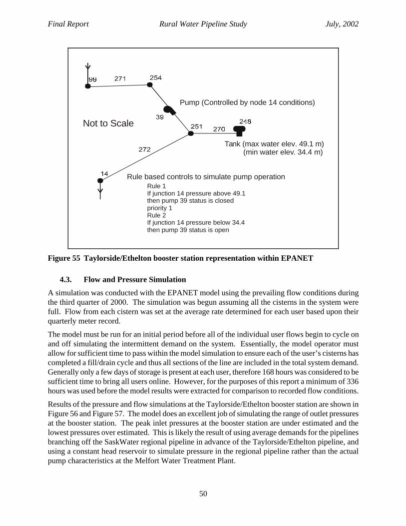
Final Report Rural Water Pipeline Study July, 2002
50
Rule 1If junction 14 pressure above 49.1then pump 39 status is closedpriority 1Rule 2If junction 14 pressure below 34.4then pump 39 status is open
Pump (Controlled by node 14 conditions)
Tank (max water elev. 49.1 m) (min water elev. 34.4 m)
Rule based controls to simulate pump operation
Not to Scale
Figure 55 Taylorside/Ethelton booster station representation within EPANET
4.3. Flow and Pressure Simulation
A simulation was conducted with the EPANET model using the prevailing flow conditions during the third quarter of 2000. The simulation was begun assuming all the cisterns in the system were full. Flow from each cistern was set at the average rate determined for each user based upon their quarterly meter record.
The model must be run for an initial period before all of the individual user flows begin to cycle on and off simulating the intermittent demand on the system. Essentially, the model operator must allow for sufficient time to pass within the model simulation to ensure each of the user’s cisterns has completed a fill/drain cycle and thus all sections of the line are included in the total system demand. Generally only a few days of storage is present at each user, therefore 168 hours was considered to be sufficient time to bring all users online. However, for the purposes of this report a minimum of 336 hours was used before the model results were extracted for comparison to recorded flow conditions.
Results of the pressure and flow simulations at the Taylorside/Ethelton booster station are shown in Figure 56 and Figure 57. The model does an excellent job of simulating the range of outlet pressures at the booster station. The peak inlet pressures at the booster station are under estimated and the lowest pressures over estimated. This is likely the result of using average demands for the pipelines branching off the SaskWater regional pipeline in advance of the Taylorside/Ethelton pipeline, and using a constant head reservoir to simulate pressure in the regional pipeline rather than the actual pump characteristics at the Melfort Water Treatment Plant.

Final Report Rural Water Pipeline Study July, 2002
51
0
10
20
30
40
50
60
336 360 384 408 432 456 480 504
Time (hours)
Pre
ssu
re (
m)
real inlet model inlet real outlet model outlet
Outlet
Inlet
Figure 56 Simulation pressure vs. measured at the Taylorside/Ethelton booster station.
0
20
40
60
80
100
120
336 360 384 408 432 456 480 504
Time (hours)
Flo
w (
L/m
in)
real flow model flow
Figure 57 Simulation flow vs. measured at the Taylorside/Ethelton booster station.

Final Report Rural Water Pipeline Study July, 2002
52
The peaks in flow at the booster station are under estimated by 10 to 15% (see Figure 57). This under estimation is likely the result of using an average flow rate drawn from the cistern at each user location. If a daily demand pattern had been programmed there would be a greater chance of the intermittent user demands coinciding in the simulation and thus producing higher peak flows at the booster station.
Figure 58 shows simulated flow and pressure at the midpoint monitoring station compared to measured pressure and flow. Note that the simulation results are not synchronized in time with the measurements. This is expected due to the method by which the simulation generates intermittent demand, and the manner in which the simulation is initiated. The magnitude and range of the pressure simulation fairly closely matches the measured pressures. A small under estimation of the peaks is evident (approx. 10%). This under estimation in pressure could stem from inaccuracy in the estimated elevation of the midpoint service connection or over estimation of the pipe roughness. The flow pattern produced by the simulation is similar to the measured pattern. The model simulation generates slightly less frequent activations (four vs. five in the period shown) with higher flow and shorter duration than the measured flows. This difference could easily be caused by the inaccuracies in the assumptions used for cistern dimensions and working volume at the midpoint.
0
10
20
30
40
50
336 360 384 408 432 456 480 504
Time (hours)
Pre
ssu
re (
m),
Flo
w (
L/m
in)
real pressure model pressure real flow model flow
Pressure
Flow
Figure 58 Pressure and flow simulation vs. measured at the midpoint.
Figure 59 shows simulated flow and pressure at the farpoint monitoring station compared to measured pressure and flow. As for the midpoint the simulation results are not synchronized in time with the measurements. Again this is expected due to the method by which the simulation generates intermittent demand, and the manner in which the simulation is initiated. The simulated pressure

Final Report Rural Water Pipeline Study July, 2002
53
range is reasonable but an under estimation of the peaks is evident (approx. 20%). Similar to the midpoint this under estimation in pressure could stem from inaccuracy in the estimated elevation of the farpoint service connection or over estimation of the pipe roughness. The flow pattern produced by the simulation is similar to the measured pattern. At this location the model simulation generates more frequent activations (five vs. three in the period shown) with lower flow and longer duration than the measured flows. Again this difference could easily be caused by the inaccuracies in the assumptions used for the cistern dimensions and working volume at the farpoint.
0
10
20
30
40
336 360 384 408 432 456 480 504
Time (hours)
Pre
ssu
re (
m),
Flo
w (
L/m
in)
real pressure model pressure real flow model flow
Pressure
Flow
Figure 59 Pressure and flow simulation vs. measured at the farpoint.
4.4. Residence Time
EPANET has the capability to simulate water residence time within the pipe distribution system, i.e. the time of travel from the water source to the delivery point. The model uses the term “water age” for the residence time. The points within a system with the longest residence time have the highest potential for water quality deterioration (loss of chlorine residual, increase in bacterial numbers). Therefore, the capability to simulate residence time is helpful to identify potential problem areas and to guide water quality monitoring programs. In conducting residence time simulations the modeller must allow a run period long enough to ensure that source water at time zero has travelled to all points in the system. After this initial start-up period the residence time to any point in the system can be tracked. The residence time will vary slightly due to the intermittent nature of the demand at a service connection.

Final Report Rural Water Pipeline Study July, 2002
54
The results of residence time simulations for flow conditions during the third quarter of year 2000 are shown in Figure 60. Note the average residence time to the booster station is approximately 60 to 70 hours. In comparison, the residence time of delivered water at the mid and farpoint monitoring stations are approximately 170 hours and 300 hours respectively. The water age in the service connection increases during no flow periods and then rapidly decreases when the cistern solenoid valve opens. When the solenoid valve opens the older water flows into the cistern from the service line and is replaced by fresher water from the main. Also note that the age of the water delivered is not simply a function of the distance to the delivery point. For example, the Jellicoe farm is closer to the booster station than the midpoint. However, due to the low rate of water use at the Jellicoe farm (single resident, minimal demand) water sits in the service connection for long periods before delivery. The Groat farm also has low water use and is located at the farthest extent of the system. As a result, the water age delivered to the Groat is 550 to 580 hrs (23 to 24 days).
Groat Farm
Farpoint
Jellicoe Farm
Midpoint
Elapse Time during Simulation
Booster Station
Figure 60 Residence times to various points – based upon the third quarter 2000 flow simulation
EPANET can easily produce plots similar to Figure 60 that illustrate water age at any selected point within the system. EPANET can also produce a contour type plot with lines of equal water age (see Figure 61). The contour type plot is less accurate, however, it is an excellent way to visualize the variation in residence time throughout the entire system. Note in Figure 61 that the extended residence time at the Jellicoe farm due to low water is indicated by the 150 hr contour in the upper left of the plot.

Final Report Rural Water Pipeline Study July, 2002
55
Figure 61 A contour representation of residence times – based upon the third quarter 2000 flow simulation

Final Report Rural Water Pipeline Study July, 2002
56
5. Discussion of Results
5.1. Flow and Pressure
Peak hourly flows recorded for the Taylorside/Ethelton branch pipeline on the discharge side of the booster station pumphouse were 128 L/min in 2000 and 142 L/min in 2001. Assuming a design flow rate of 4.54 L/min (1 ImpGal/min) for each user, the maximum flow rate that would be generated by the 36 users downstream of the booster station is 163 L/min. Therefore, the pipeline is approaching design capacity during maximum hourly flow. Peak hourly flows for the Lucky Lake system could not be determined due to the datalogger synchronization problem.
The peak flow rates recorded on the Taylorside/Ethelton system at the user sites during cistern filling were typically in the range of 10 to 17 L/min which is substantially higher than the typical design flow rate of 4.5 L/min. The peak flow rates recorded on the Lucky Lake North system at the user sites during cistern filling were typically in the range of 6 to 8 L/min, however, flows at the midpoint occasionally approached 20 L/min.
A summary of the peak and average flow characteristics measured for the Taylorside/Ethelton booster station are shown in Table 3. The ratios of peak hourly flow and peak daily flow to average flows that were measured for this rural system are large in comparison to urban systems. For example, the average ratios of peak hourly flow and peak daily flow to average flow in Saskatoon were 3.3 and 2.0 respectively during 1998 to 2000.
Table 3 Taylorside/Ethelton booster station flow characteristics
Year 2000 Year 2001 Average Max hourly flow (L/min) 128 142 135 Max daily flow (L/min) 51 55 53 Average flow (L/min) 24 32 28 Max. hrly / Avg. 5.3 4.4 4.8 Max. daily / Avg. 2.1 1.7 1.9
In urban water distributions systems peak demand periods are primarily caused by lawn watering during hot summer months. Periods of high demand on rural systems can occur at several times of the year depending upon agricultural activities. On the rural systems monitored high demand occurred during hot dry weather as expected, but also during spraying operations in the spring and fall, and during the winter due to cattle watering.
Users at the furthest extents of a rural branch pipeline have a strong influence on the system pressure. When these users receive water large headlosses can occur due to the smaller diameter mains feeding these locations. Evidence of these effects could be seen at the farpoint monitoring stations on each of the pipelines studied, however the effects were far more prominent on the Lucky Lake system.

Final Report Rural Water Pipeline Study July, 2002
57
The float switch setting in the users’ cisterns can have a strong influence on the water demand pattern exerted on the delivery system. If a large draw down is required before the switch actuates then less frequent longer duration flows will occur as was evident for the Taylorside/Ethelton system. If only a small draw down is permitted then very frequent short duration flows will occur as was evident for the Lucky Lake North system.
EPANET or similar computer models can provide a reasonable simulation of a rural water pipeline’s hydraulic behaviour with only a small amount of input data. EPANET or a similar model could be used to assess the impact of a pipeline expansion such as the additional of users or changes in pumping capacity.
5.2. Water Quality
Peaks in DOC, turbidity, particle count, and bacterial count in the pipelines and source waters were observed in the early spring (likely corresponding to runoff and/or overturn in reservoirs), and in late summer when water temperature is at a maximum causing maximum biological activity.
Water temperature in the pipelines and at the source was observed to follow a yearly cycle with peak temperature occurring in late summer (generally August) and minimum temperature occurring in early spring (generally March).
The deep burial (> 2.5 m) of rural pipelines under relatively undisturbed land, and the very long retention times in the system (often over a week) cause the water to be cooled to the subsurface ground temperature. This cooling effect causes the water temperatures to be well below the prevailing surface water temperature at the pipeline source. The cooling effect also keeps the water temperature below the reported threshold for biofilm development (15 deg C) during the vast majority of the year.
The observed peaks in DOC levels in late summer/early fall coincide with peak subsurface temperatures and thus the peak water temperatures in the pipeline. These concurrent conditions represent the largest potential for water quality deterioration during the year. The two instances of low chlorine residual in the Taylorside/Ethelton system that were observed during the study both occurred in late summer/early fall period.
Chlorine residual is more difficult to maintain during peak occurrences of DOC and high water temperature. Service connections with limited water use at any position in the system, and areas on the peripheral of the system are particularly susceptible during these periods due to long retention times. EPANET or a similar model can serve as a valuable tool to identify these areas and to help plan water quality sampling programs.
No strong evidence of significant deterioration in water quality along the pipelines was discovered. This may be due to the inherent scatter in many of the water quality parameters measured and the cooling effect of the subsurface ground temperatures causing suppression of biological activities and chemical reactions.
During the periods of low chlorine residual on the Taylorside/Ethelton pipeline there was evidence of increased bacterial counts in the pipeline. Fortunately, these episodes were of limited duration and the bacterial counts did rise to unacceptable levels.

Final Report Rural Water Pipeline Study July, 2002
58
It should be noted that the water quality measurement results presented in this report are for the service connections supplying the farmsteads (that were monitored) rather than the users’ cisterns. Water quality measurement results for cisterns or in-house piping systems could give very different results. The water held in a cistern and in the plumbing will have even longer retention times than the service connection and will also have a much higher water temperature. As a result, water quality in the cistern is likely to have increased potential for deterioration.
5.3. Biofilm Development
The pipe excavation investigations on the Taylorside/Ethelton branch pipeline produced no evidence of significant biofilm development. These findings further support the contention that the cooling effect of the subsurface ground temperature has a very strong mitigating affect upon biological activity in the pipeline. Despite the presence of DOC for substrate and bacteria for inoculum there is only a brief period each year when water temperature in the pipeline approaches threshold temperatures for biofilm development. The temperature effect combined with the presence of chlorine residual appears to be effectively preventing biofilm development in the system.
The pipe excavation investigations on the Lucky Lake North branch pipeline produced some evidence of limited biofilm development in the raw water pipeline. Conditions in the Lucky Lake North pipeline are more favourable for biological activity than in the Taylorside/Ethelton pipeline. In particular, the water temperatures are slightly higher, there are higher bacterial counts indicating ample bacteria for inoculum, and of course there is no chlorine residual to control growth. Despite these more favourable conditions, the biofilm development at the Lucky Lake locations was limited and smaller in magnitude than has been reported for urban system (LeChevallier et al., 1987). Again it is likely that cool water temperature, and perhaps the pipe material, play an important mitigating role in limiting biofilm development.
6. Recommendations
The following is recommended based upon the results of the rural water pipeline flow and water quality study.
Treated water pipelines should be routinely monitored for chlorine residual and bacterial counts. The frequency of monitoring should be increased during periods of the year when there is the greatest potential for water quality deterioration. The most vulnerable periods are in the spring during turnover in reservoirs, and during late summer when there is maximum water temperature and peak biological activity.
Care must be taken when sampling water in a pipeline system. Water drawn from a user cistern or in-house plumbing will not be representative of the service connection and pipeline conditions. Sampling ports should be installed on the inlet line to the cistern to allow representative samples to be drawn from the pipeline system.
A study of the water in cisterns should be undertaken to investigate whether significant deterioration in quality occurs after the water is delivered from the pipeline. Concurrent sampling of the service connection and the cistern would allow a comparison.

Final Report Rural Water Pipeline Study July, 2002
59
Tracking the water temperature in the distribution system is recommended as an aid to identifying the most vulnerable times of the year for water quality deterioration.
Treated water pipelines should be closely monitored if a change in source water is required. If adverse water quality effects are detected in the system the operators must be prepared to react quickly to take mitigating actions.
A hydraulic model of a pipeline system constructed with software package such as EPANET should be used to identify the locations that have the highest potential for water quality deterioration. The hydraulic model should be based upon flow records and properties of the system as constructed.
A hydraulic model constructed within EPANET or a similar software package should be used as an aid to the design of new rural pipeline systems and to evaluate the effect of additional users on an existing system. The effects of alternative pumping facilities, system layout and control devices can be easily checked using a computer based hydraulic model.
All pipeline pumping facilities should be equipped with instrumentation to allow routine collection of pressure and flow data. The instrumentation should have the capability to indicate daily averages as a minimum. Data collected to allow calculation of hourly or sub-hourly averages is preferrable. Pressure and flow data are valuable aids to troubleshooting system problems in advance of failures and for cross checking with meter readings.
All rural pipeline systems should have a regular program of flushing of mains and service connections. Service connections should not be flushed into the users cistern. A bypass connection should be installed at each service connection between the water meter and the cistern. The bypass could also be used for water quality sampling purposes.
The water from mains and service connections during flushing operations should be analysed for HPC and coliform counts to assess biofilm formation in the system. If excessive counts are obtained the system should be subjected to further flushing and then be re-sampled.
The potential for biofilm formation and water quality deterioration in rural pipelines with higher water temperatures should be investigated. The pipelines investigated in this study may not be representative of all conditions encountered in Saskatchewan or at other locations in Canada.
A better method of assessing biodegradable dissolved organic carbon should be investigated for use in future studies. The 28-day incubation period utilized in this study proved to be cumbersome and the results produced were quite variable.

Final Report Rural Water Pipeline Study July, 2002
60
7. Acknowledgements
The following agencies, groups and individuals contributed to the rural water pipeline study. Their cooperation and contributions are gratefully acknowledged. By working together we always have a better chance of achieving our collective goals.
Saskatchewan Association of Rural Water Pipelines - Project Sponsor
Agri-Food Innovation Fund - Financial Support
Rural Water Development Program - Financial Support
Canadian Adaptation & Rural Development Program - Financial Support
Natural Sciences and Engineering Research Council of Canada - Financial Support
University of Saskatchewan - In Kind and Financial Support
PFRA, Agriculture and Agri-Food Canada - In Kind Support
Melfort Rural Pipeline Association - Datalogger Equipment, Flow Records, Access to sites
Coteau Hills Pipeline Association - Datalogger Equipment, Flow and Pressure Records, Access to sites
Environment Canada - Laboratory Services, Access to UV Microscope
Saskatchewan Health – HPC Sample Bottles and Analyses
Saskatchewan Water Corp. - Access to Facilities, Flow Records
Saskatchewan Research Council – Loan of On-line Turbidimeters
G. Audette, W. Audette, Tullis, Eremenko, Jellicoe, and Groat families - Access to sites

Final Report Rural Water Pipeline Study July, 2002
61
8. References
Clark R.M., Grayman W.M., Males R.M. and Hess A.F. (1993) Modeling Contaminant Propagation in Drinking-Water Distribution Systems. Journal of Environmental Engineering, Vol. 119, No. 2, pp. 349-364.
Corkal, D. (1997). Prairie Water Quality Problems, Water Quality Matters Fact Sheet, PFRA, Agriculture and Agri-food Canada, December, 1997, Saskatoon, Saskatchewan, 5p.
Escobar I.C. and Randall A.A. (1999) Influence of Nanofiltration on Distribution System Biostability. JAWWA, Vol. 91, No. 6, pp. 76-89.
Laurent P., Servais P., Prevost M., Gatel D. and Clement B. (1997) Testing the SANCHO Model on Distribution Systems. JAWWA, Vol. 89, No. 7, pp. 92-103.
LeChevallier M.W., Babcock T.M. and Lee R.G. (1987) Examination and Characterization of Distribution System Biofilms. Applied and Environmental Microbiology, Vol. 53, No. 12, pp. 2714-2724.
Piriou P., Dukan S. and Kiene L. (1998) Modelling Bacteriological Water Quality in Drinking Water Distribution Systems. Water Science and Technology, Vol. 38, No. 8-9, pp. 299-307.
Pochylko D. and Morrison W. (2000) Rural Pipeline Installation on the Canadian Prairies. Small Drinking Water and Wastewater Systems Conference, National Sanitation Foundation International and Rural Water Research and Education Foundation, January 12 – 15, 2000, Pheonix, AZ.
Pochylko D., Arndt R., Audette G., Sheldon C. and Verhelst T. (2000) Saskatchewan Rural Water Pipeline Organization and Administation. Small Drinking Water and Wastewater Systems Conference, National Sanitation Foundation International and Rural Water Research and Education Foundation, January 12 – 15, 2000, Pheonix, AZ.
Porter K. and Feig Y. (1980) The Use of DAPI for Identifying and Counting Aquatic Microflora. Limnology and Oceanography, Vol. 25, No. 5, pp. 943-948.
G. Putz (2000) Literature Review: Potential for Water Quality Deterioration in Rural Pipelines" Project report for Saskatchewan Association of Rural Water Pipelines and PFRA, Agriculture and Agri-Food Canada, Saskatoon, Saskatchewan, 27 p.
Rossman L.A., Clark R.M. and Grayman W.M. (1994) Modeling Chlorine Residuals in Drinking Water Distribution Systems. Journal of Environmental Engineering, Vol. 120, No. 4, pp. 803-819.
Servais P., Anzil, A. and Ventresque, C. (1989) Simple Method for Determination of Biodegradable Dissolved Organic Carbon in Water. Applied and Environmental Microbiology, Vol. 55, No. 10, pp. 2732-2734.
Servais P., Laurent P., Billen G. and Gatel D. (1995) Development of a model of BDOC and Bacterial Biomass Fluctuations in Distribution Systems. Revue des Sciences de L'eau, Vol. 8, No. 4, pp. 427-462.
Sketchell, J., Peterson H.G., Christofi N. and Brandt G. (1993). Dissolved Organic Carbon in Surface Drinking Water Reservoirs in Saskatchewan, Proceedings of the 5th National Conference on Drinking Water: Disinfection Dilemma, Winipeg, MB., American Water works Association, Denver, CO., pp. 365-382.

Final Report Rural Water Pipeline Study July, 2002
62
Appendix A Photographs of Monitoring Locations
Figure 62 Taylorside/Ethelton midpoint monitoring location.
datalogger
flowmeter
turbidimeter
pressuretransducer sampling
port
datalogger
flowmeter
turbidimeter
pressuretransducer sampling
port
Figure 63 Taylorside/Ethelton midpoint monitoring set-up.

Final Report Rural Water Pipeline Study July, 2002
63
Figure 64 Taylorside/Ethelton farpoint monitoring location.
Figure 65 Taylorside/Ethelton farpoint monitoring set-up.

Final Report Rural Water Pipeline Study July, 2002
64
Figure 66 Lucky Lake North midpoint monitoring location.
datalogger
storage tanks
Figure 68 Lucky Lake farpoint monitoring set-up.
sampling port
pressure transducer
flowmeter
water meter pressure reducer
regulator
Figure 67 Lucky Lake farpoint monitoring set-up close-up.

Final Report Rural Water Pipeline Study July, 2002
65
Figure 69 Lucky Lake North farpoint monitoring location.
Figure 70 Lucky Lake farpoint monitoring set-up close-up.
Figure 71 Lucky Lake farpoint monitoring set-up.

Final Report Rural Water Pipeline Study July, 2002
66
Appendix B EPANET Model and Data File
The EPANET model set-up files and users manual obtained from the USEPA website are included on the CD attached to the report.
The EPANET model file representing the Taylorside/Ethelton branch pipeline system and flow conditions for the third quarter of year 2000 is included on the attached CD. The file name is Taylorside3Q2000.net.