Rule Base Design of Antecedent Fuzzy Variable for I DMT Relay

4.1 Introduction

4.2 Characteristics of IDMT Relay

4.3 Membership Function

4.3.1 Data Driven Fuzzy Variable Design

4.3.2 Point Membership Function

4.4 Rule Base Design

4.5 Rule Base Inference

4.6 Fuzzy Tunned Neural Network

4.6.1 Network Design for IDMT Relay

4.6.2 Neural Network Training

4.7 Simulation Result

4.8 Discussion

"It was the best of time ,it was the w orst of times, it was the age of wisdom ,it was the age of

fool shness ,it was the epoch of believe, it was the epoch of increduality.it was the season of light ,it

was the season of darkness ,it was the spring of hope ,it was the w inter of despair ,we had every

thin j before us ,we were all going d irect to heaven , we w ere all going direct to the other way -in

short ,the period was so fa r like the present period .that some of its noisiest authorities insisted on

its being received, for good or fo r e v il . In the superlative degree of comparison o n ly ."

Charles Dickens

A tale of Two cities ,1859

Chapter 4 .

Rule Base Design of Antecedent Fuzzy Variable for IDMT Relay

4.1 IntroductionIn the design of a power system, three aspects are generally considered namely normal

o p e r a tio n , prevention of electrical failure and the reduction of damaging effects caused by an

e le c tr ic a l failure [62], There should be devices which will disconnect the faulty equipment of the

p o w er system with the help of circuit breakers (C.B.) associated with the said equipment, when it

su ffer s f r o m a short circuit or behaves in an abnormal fashion that might cause damage to the

e q u ip m e n t or interfere with the effective operation of the rest o f the power system [62,77].

Fig.4.1 shows the location o f a conventional relay and the sequence of events leading to the

final disconnection of faulty equipment [77]. These events are :

C.B.

Fig. 4.1 Conventional Relay location in power system

(i) Detection of primary condition.

(ii) Processing of the detected information.

(iii) Resulting chain of commands to C.B.

The power system elements generally consist o f generators, transformers, transmission

lines, cables, synchronous and induction motors and switch gears. Each o f them develop some

faults sooner or later.

Extensive work had been done in this field and also in the application of on-line digital

and analogous computers to power system protection with the development o f low cost micro

computer system/micro processor, the economics are changing at a fast rate and investigators are

trying to develop dedicated digital protection schemes which closely imitate the existing relaying

practices [50]. Each relaying function is served by a separate unit which requires a highly parallel

distributed processor network, in which each processor is strictly dedicated to a particular protective

function.

With the advent of fuzzy systems and Neural Network an expert system or adaptive system

may be developed to act as an digital relay [72]. The concept of fuzzy sensor as a relay may be used

to develop the above system . The inverse definite time relay characteristics or data may be fuzzified

and after a required fuzzy mathematical manipulation or rule based reasoning the result may be

defuzzified to obtain the prescribed characteristic of relay performance [106]. The antecedent or input

variable (one or two input variables) may be fuzzified from its crisp or singleton value and an NN is

trained to design the membership function of input or antecedent variables [85-88].

4.2 Characteristics of IDMT relaySingle input protection schemes are actuated by a single input taken from the power systems

in abnormal (Faulty) condition [62], The schemes work basically either on presence or on absence of

selected input quantity. These relays operate only on the basis of the system current exceeding a

normal value.

Inverse time over current relay type CDG11 manufactured by GEC Alsthom is preferred for

fuzzifying its rating [56]. These relays are available in the standard current setting ranges of 50-200%,

20-80% and 10-40% of 1A or 5A. The 5A rating is considered here. The technical data are :

Current Rating = 1A or 5A

IDMT Setting = 50-200% in seven equal steps of 25%

20-80% in seven equal steps of 10%

10-40% in seven equal steps of 5%

Operating Time = 0-3 seconds or at 10 times

0-1.3 seconds J current settings

The relay characteristics are adjusted to have a definite minimum time of operation for plug

setting multiplier higher than 20 in general. Thus the actual relay characteristic becomes an inverse

characteristic below this value of Plug Setting Multiplier (PSM) and a straight line above this value.

T h e plug setting steps are calibrated in terms of time setting multiplier (TSM) which is defined as :

Actual - operating - time - o f - relay Calibrated - operating - time - fo r - a - particular - PSM

Fig. 4.2 shows a standard IDMT characteristics curve drawn in logarithmic scale between

PSM and operating time .The original curve of IDMT relay i.e. CDG11 obtained from the manual of

GEC Alsthom, India is attached in “appendix A” of this thesis. For standard IDMT relays, the

r e c o m m e n d e d expression for time current relationship is given by -

0.14/ 0 .0 2 _ 1

Here T = Operating time of relay and I = Operating current of relay.

Fig. 4.2 Characteristics curve of IDMT relay

The static time over current relays generally require an auxiliary current transformer (C.T.) to

reduce the main C.T. secondary current still further by 10 times . Static over current relay essentially

consists of a rectifying circuit, an integrating circuit and two level detector arrangements (see Fig.

4.3). Fig. 4.4 shows the proposed fuzzy sensor scheme for IDMT over current relay [93] . These

relays operate after a fixed interval of time, after the fault current (If) exceeds the pick up current (Ip)

level. The working behavior of IDMT relay would be governed by the characteristics curve shown •n Fig. 4.5.

Inp ut

Fig. 4.3 Static over current

Plug Setting

Fig. 4.4 Proposed scheme of O.C. Relay

4.3 Membership FunctionCharacteristic curve of IDMT relay is shown in Fig. 4.5, oiginal curve o f GEC Alsothm India

is attached in Appendix A. This IDMT relay is fuzzifled as shown in Fig. 4.5 with three membership

function small, medium, high for plug setting multiplier (PSM) and its corresponding operating time.

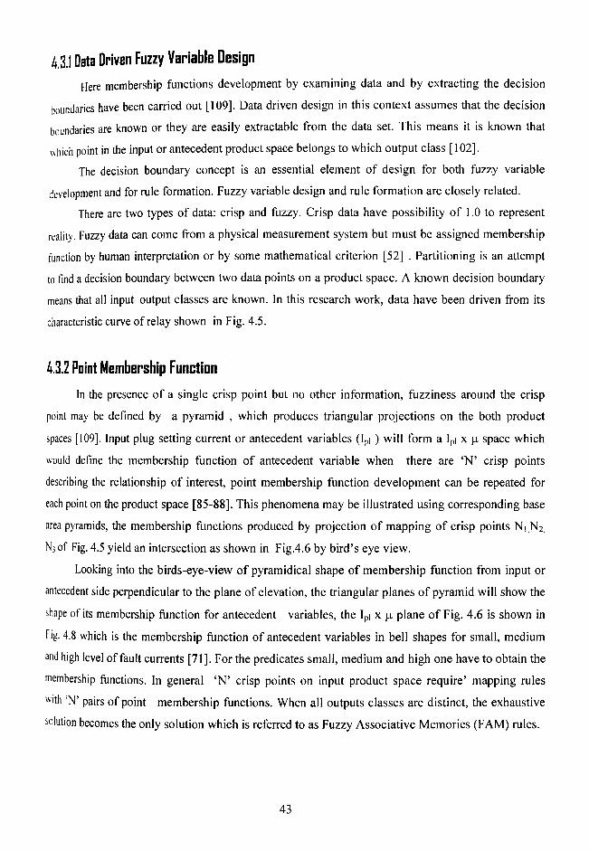
4.3.1 Data Driven Fuzzy Variable DesignHere membership functions development by examining data and by extracting the decision

b o u n d a r ie s have been carried out [109]. Data driven design in this context assumes that the decision

b o u n d a r ie s are known or they are easily extractable from the data set. This means it is known that

w h ic h point in the input or antecedent product space belongs to which output class [102].

The decision boundary concept is an essential element of design for both fuzzy variable

d e v e lo p m e n t and for rule formation. Fuzzy variable design and rule formation are closely related.

There are two types of data: crisp and fuzzy. Crisp data have possibility of 1.0 to represent

reality. Fuzzy data can come from a physical measurement system but must be assigned membership

function by human interpretation or by some mathematical criterion [52] . Partitioning is an attempt

to find a decision boundary between two data points on a product space. A known decision boundary

means that all input-output classes are known. In this research work, data have been driven from its

characteristic curve of relay shown in Fig. 4.5.

4.3.2 Paint Membership FunctionIn the presence of a single crisp point but no other information, fuzziness around the crisp

point may be defined by a pyramid , which produces triangular projections on the both product

spaces [109]. Input plug setting current or antecedent variables (Ipi ) will form a Ipi x )u space which

would define the membership function of antecedent variable when there are ‘N ’ crisp points

describing the relationship of interest, point membership function development can be repeated for

each point on the product space [85-88]. This phenomena may be illustrated using corresponding base

area pyramids, the membership functions produced by projection of mapping of crisp points Ni N2;

N3 of Fig. 4.5 yield an intersection as shown in Fig.4.6 by bird’s eye view.

Looking into the birds-eye-view of pyramidical shape of membership function from input or

antecedent side perpendicular to the plane of elevation, the triangular planes of pyramid will show the

shape of its membership function for antecedent variables, the Ipi x y. plane of Fig. 4.6 is shown in

Fig. 4.8 which is the membership function of antecedent variables in bell shapes for small, medium

and high level of fault currents [71]. For the predicates small, medium and high one have to obtain the

membership functions. In general ‘N’ crisp points on input product space require’ mapping rules

with ‘N’ pairs of point membership functions. When all outputs classes are distinct, the exhaustive

solution becomes the only solution which is referred to as Fuzzy Associative Memories (FAM) rules.

"Oeoo<L><Z3

60C

oa0

3 4 5 6 7 8 9 10

Multipliers of plug Setting Current

20

Fig 4.6 Birds -eye-view of Membership Function for antecedent variable

Fig. 4.7 depicts the design interface of antecedent variables for IDMT relay. This interface is

used to design the input/output fuzzy variable and fuzzy inference system for rule based sensor This

FIS received plug setting current as input and produces operating time as an output

Fig. 4.8 illustrates the membership function of antecedent variable (i.e. plug setting current)

[94] preferring bell shaped curve, which is most widely used membership curve for input variable.

The choice of shape of membership function depends on the reasoning skill o f an expert person.

Fig 4.7 Fuzzy inference engine designed for IDMT relay

The designed membership function of consequent variable [94] are shown in Fig. 4.9 for its

lo w , m e d iu m and high linguistic variable in given universe o f discourse.This membership is obtained

a c c o r d in g to the membership curve of antecedent variable of IDMT relay shown in Fig. 4.5.

4 6 8 10 12 14 16 18 20input variable 'plug-setfing-current"

Fig. 4.8 Membership function in bell shape of antecedent variables

Membership ftncfon plots P^P0*^ - 181

oulput variable ‘fcperafrig-ime”

Fig. 4.9 Membership function in triangular shape of consequent variables

44 Rule Base DesipAccording to the characteristics curve of IDMT relay FAM rules can be summarized in the

f o l l o w i n g table [25].

The above FAM rules can be written in form of IF -THEN as given below.

IPi*Ps -------------------------------------►

I p i * P m -------------------------------------------- ► O t . P m

I p i* P h ----------------------------------------------► O t . P l

...(4.1)

These rules are referred to as fuzzy associative memories (FAM) rules. The rule base design interface

obtained from the MATLAB software is shown in Fig. 4.10 for three FAM rules.

2. If (plug-setting-current is M edium ) then (operating-time is M edium ) (1 )3. If (plug-setting-current is H igh) then (operating-time is low] (1)

plug-tetting-current

aa —

operating-tim e is

MediumHighnone

Fig. 4.10 Rule base design for inference engine

lowMedium U f

-d

FAM R ulel: IF plug setting current level is small THEN operating time for relay is High.

FAM Rule2 :IF plug setting current is Medium THEN operating time for relay is Medium.

FAM Rule3 : IF plug setting current is High THEN operating time of relay is Low.

In equation 4.1 Ip,

Ot

Ps

Pm

P h

Plug setting current level.

Operating time of relay

Predicate Small

Predicate Medium

Predicate High

pL = Predicate Low

# = Symbol for ‘IS’

_ > = Symbol for ‘THEN’

In the context of fuzzy system design, uncertainties are represented by membership functions

and b y their individual properties. The above discussions mainly included the determination of the

n u m b e r and location of membership functions. One can also examine their shape without being

c o n c e r n e d about their number and location on the universe of discourse.

The geometrical shape of membership function is the characterization of uncertainty in the

corresponding fuzzy variable. Nevertheless, the shape of a membership function cannot be formed

arbitrarily because arbitrary design can produce unpredictable results in the basic fuzzy inference

algorithm. The triangle and trapezoid are the two geometric shapes commonly used to represent

uncertainties [52], The height of a membership function determines the maximum value of

membership function. In Fig.4.5 the height of membership functions are equal with equal amount of

fuzziness (i.e. 100%) .From the basic definition of membership function , the width of occupancy is

the measure of fuzziness. In Fig.4.5 membership function Ni is most fuzzy than rest of the two N2 &

N3, again N3 has least fuzziness [106,109].

From the inverse characteristics of relay (Fig.4.5) one can see that for low fault current level

the operating time of relay would be high and vice-versa.

A fuzzy set defines a point in a fuzzy universe of discourse .A fuzzy system defines a

mapping between two fuzzy universe of discourses. A fuzzy system ‘S’ maps fuzzy sets to fuzzy sets.

Thus a fuzzy system ‘S ‘is a transformation S: Ipin —► Otp .The n-dimensional units hypercube Ip"

contains all the fuzzy subsets of the input universe of discourse [106].

Ipi" = (Ipll, Ipl2,IpL3,.................. Ipin) ...(4.2)0pt contains all the fuzzy subsets of the output universe of discourse.

Opt = (Ou .Oq .Oo, ..............Otn) ...(4.3)

They map close inputs to close outputs, which are referred as fuzzy associative memories or FAMs,

The FAM rule [109].

IF ‘Isp,’ is ‘Ps ‘ THEN Ost IS PH .... (4.4)

May be encoded by (PS; Ph)

In general a FAM system F: Inpi-----► Opt encodes and processes in parallel a FAM bank of FAMrules.

(psi, Phi) , (PS2> Pin), (Psa, Pro).................(Psm, Phm) . • -(4.5)

Fuzzy systems estimate functions with fuzzy set samples (Psi, PhO , neural samples use

numerical-point samples. Engineers sometimes call the fuzzy set association (Psi, Phi) a “rule” . Here

p s , is r e f e r r e d as antecedent term and P h i is referred as consequent term. The antecedent variables

w ith r e fe r r e d to membership function (Fig.4.5) would be -

T h e r e s p e c t i v e consequent variable would be -

( 0 H„ , O h q , O h ,3 , O h ,4 , O m „ , 0 Mt2 , 0 % , 0 \ , O l , i , 0 La , O ' o , O l „ ) . . . ( 4 . 7 )

4.5 Rule Base InferenceThree rules obtained from FAM rule table can be viewed from the rule viewer for different

plug setting current as shown in Fig. 4.11 (a), (b).Fig. 4.11 (a) shows the rule firing process for Ipl = 7

Amp, for this plug setting current only the second rule is firing and giving fuzzy data as shown in this

figure at the right side .In the same manner Fig. 4.11(b) shows rule firing process for Ipi = 10 Amp .

Simulated characteristics curve of IDMT relay ,input as plug setting current and output as

operating time is shown in Fig. 4.12 .This curve is not smooth as compare to the curve in Fig. 4. 5,

this is due to less number of rules (only 3 rules). By increasing the number o f rules this problem may

be overcome, but initially only 3 rules has been considered to check the performance of IDMT relay

as fuzzy relay or fuzzy sensor. From the curve shown in Fig.4.12 it is clear that, the simulated version

of characteristics curve of IDMT relay also satisfied the rules of original curve .In this curve it is clear

that if will increase plug setting current then operating time will decrease. Hence it’s nature is

analogous to the original IDMT curve.

phJQ-setinQ-cuFrents 7opera#ng-time >■ 0.46

0.3 0.9

Fig. 4.11 (a) Rule base inference process for Ipi 7 Amp

operaSng-fme = 0.462

\

/ \v

/

2 20A

Fig. 4.11 (b) Rule base inference process for Ipi = 10 Amp

pfcig-setling-eurrent

Fig. 4.12 Simulated characteristics curve of IDMT relay

4.G Fuzzy Tunned Neural Network TrainingThe fuzzified antecedent multiplier of plug setting current level Ipi (Equation 4.14) are input to

the neural network.

Antecedent variables for IDMT relay have been designed using fuzzy logic technique and the

same variables are being used for NN training [79]. The results must comply the performance of

IDMT relay. The weight of input to hidden layer (ith layer to j th layer) would provide us the trained

values of antecedent variables. This is the objective of this research. The membership functions for

antecedent variables of IDMT relay trains an ANN for several iteration.

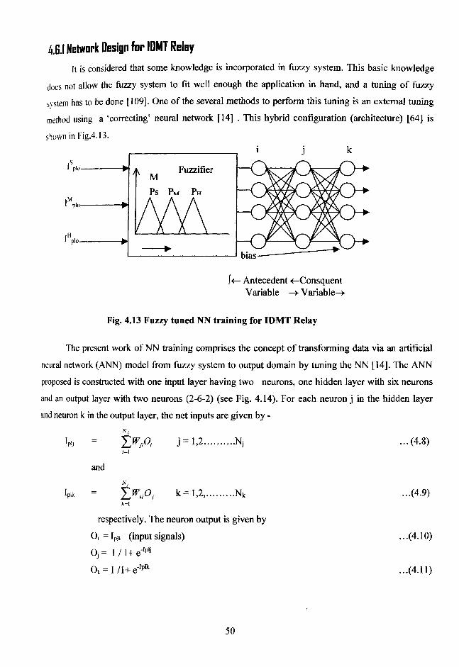
411 Network Design for IDMT RelayIt is considered that some knowledge is incorporated in fuzzy system. This basic knowledge

does not allow the fuzzy system to fit well enough the application in hand, and a tuning of fuzzy

svstem has to be done [109]. One of the several methods to perform this tuning is an external tuning

method using a ‘correcting’ neural network [14] . This hybrid configuration (architecture) [64] is

shown in Fig.4.13.

1 j k

bias-

f<- Antecedent Consquent Variable -> Variable-*

Fig. 4.13 Fuzzy tuned NN training for IDMT Relay

The present work of NN training comprises the concept of transforming data via an artificial

neural network (ANN) model from fuzzy system to output domain by tuning the NN [14]. The ANN

proposed is constructed with one input layer having two neurons, one hidden layer with six neurons

and an output layer with two neurons (2-6-2) (see Fig. 4.14). For each neuron j in the hidden layer

and neuron k in the output layer, the net inputs are given by -

pij

Ip lk

and

I y p ,

I X 0 ,k=1

j = 1,2 . •N i

k = 1,2, •Nk

respectively. The neuron output is given by

O; = IpH (input signals)

Oj = l / l + e Iplj

Ok = 1 /1+ e‘Iplk

...(4.8)

...(4.9)

...(4.10)

...(4.11)

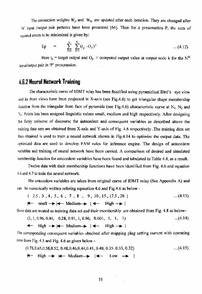
The connection weights Wjj and Wkj are updated after each iteration. They are changed after

•N' input /output pair patterns have been presented [64]. Then for a presentation P, the sum of

squared errors to be minimized is given by:

E P = f . i^p -O p f . . . ( 4 . 12 )N = 1 t = l

Here tp = target output and Op = computed output value at output node k for the Nth

input/output pair in ‘P’ presentation.

4.E.2 Neural Network TrainingThe characteristic curve of IDMT relay has been fuzzified using pyramidical Bird’s eye view

and its front views have been projected in X-axis (see Fig.4.6) to get triangular shape membership

function from the triangular front face of pyramids (see Fig.4.6) characteristic curve at Ni; N2 and

N3. Points has been assigned linguistic values small, medium and high respectively. After designing

the fuzzy universe of discourse for antecedent and consequent variables as described above the

training data sets are obtained from X-axis and Y-axis of Fig. 4.6 respectively .The training data set

thus obtained is used to train a neural network shown in Fig.4.14 to optimize the output data. The

optimized data are used to develop FAM rules for inference engine. The design of antecedent

variables and training of neural network have been carried. A comparison of desired and simulated

membership function for antecedent variables have been found and tabulated in Table 4.4, as a result.

Twelve data with their membership functions have been identified from Fig. 4.6 and equation

4.6 and 4.7 to train the neural network.

The antecedent variables are taken from original curve of IDMT relay (See Appendix A) and

can be numerically written refering eqnuation 4.6 and Fig.4.6 as below -

( 2.5, 3 ,4 , 5 , 6 , 7 , 8 , 9 , 10 , 15 , 17.5 , 20 ) ...(4.13)

j*— small —► |-4— Medium—► | <— High —► |

these data are treated as training data set and their membership are obtained from Fig. 4.8 as below-

(1,1,0.96,0.44, 0.28,0.91,1,0.96, 0.001, 1, 1, 1) ...(4.14)

ft— High —► \4— Medium—► | *4— High —► |

The corresponding consequent variables obtained after mapping plug setting current with operating

time from Fig. 4.5 and Fig. 4.6 as given below -

(0.78,0.65,0.58,0.52, 0.48,0.46,0.44,0.41, 0.40, 0.35. 0.33, 0.32) ...(4.15)

i*— High —► (4— Medium—► \<— Low —► |

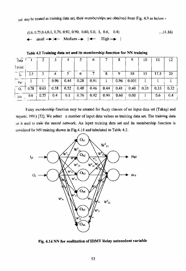
and may be treated as training data set, their memberships are obtained from Fig. 4.9 as below -

(0.6,0.75,0.4,0.1,0.76,0.92,0.90, 0.60,0.0, 1,0.6, 0.4) ...(4.16)

small —► \<4— Medium—► | <4— High—► |

Table 4.2 Training data set and its membership function for NN training

Data

Point

1 2 3 4 5 6 7 8 9 10 11 12

Ipi 2.5 3 4 5 6 7 8 9 10 15 17.5 20

Mipi 1 1 0.96 0.44 0.28 0.91 1 0.96 0.001 1 1 1

ot 0.78 0.65 0.58 0.52 0.48 0.46 0.44 0.41 0.40 0.35 0.33 0.32

Mot 0.6 0.75 0.4 0.1 0.76 0.92 0.90 0.60 0.00 1 0.6 0.4

Fuzzy membership function may be created for fuzzy classes of an input data set (Takagi and

Hayashi, 1991) [72]. We select a number of input data values as training data set. The training data

set is used to train the neural network. An input training data set and its membership function is

considered for NN training shown in Fig.4.14 and tabulated in Table 4.2.

Fig. 4.14 NN for realization of IDMT Relay antecedent variable

W e ig h ts for input to hidden and hidden to output layers are obtained from equation 4.14 and 4.16

after modification as shown in Table 4.3.

Table 4.3 The initial assigned weights to the paths connecting inter layer nodes

Input to hidden inter

layer weights

Assigned values to

input to hidden layer

elements

Hidden to output layer

weights

Assigned values to

hidden to output layer

elements

.I- w 'n 0.35 w 2„ 0.45

I W',2 0.75 w 212 0.9

W‘,3 0.25 w 2I3 0.45

W',4 0.01 w 214 0.01

1 W',5 0.45 w 215 0.35

w ‘,« 0.75 w 216 0.35

w '2, 0.75 w 221 0.85

W a 0.45 W222 0.80

W 23 0.01 W223 0.01

w '24 0.95 W224 0.01

w '25 0.01 W225 0.35

w '26 0.45 W226 0.01

The FAM rules may be developed in Neuro-linguistic form [109] (see Table 4.2 )

FAM Rule 1 : IF plug setting current level is 2.5 Amp with 1 fuzzy membership function (Fuzzy

grade of truth) THEN Relay Operating time is 0.78 second with 0.6 membership function (fuzzy

function grade of truth)

FAM Rule 2 : IF plug setting current level is 7Amp with 0.91 membership function THEN Relay

operating time is 0.46 second with 0.92 membership function

FAM Rule 3 : IF plug setting current level is 15 Amp with 1.0 membership function THEN relay

operating time is 0.35 second with 1.0 membership function.

4.7 Simulatinn ResultsANN shown in Fig. 4.14 is trained after assigning initial weights from Table 4.3 and using

training data given in Table 4.2, obtained results are tabulated in Table 4.4 and Table 4.5 , containing

input and output data set for its desired and simulated values. The error thus obtained is in

a c c e p t a b le range. It is tried to illustrate a conceptual design of the antecedent variables for the IDMT

r e la y t o develop it as a fuzzy sensor for power system protection. The training performance curve of

n e u r a l network is shown in Fig.4.14. The training goal was met after 100 epochs.

Fig. 4.14 Performance of neural netwok shown in Fig.4.13

4.8 DiscussionThe characteristic curve of IDMT relay has been fuzzified to design the antecedent variables

o f IDMT relay as fuzzy sensor. This curve has also fuzzified referring the theories like bird’s-eye-

v i e w and point membership function of input /output data sets.

The fuzzified antecedent variables obtained from Fig. 4.5 is used to train the neural network.

The twelve data, four from each linguistic values i.e. small, medium and high respectively along with

their corresponding membership functions are considered for training the Neural Network .The

desired values of antecedent variables are obtained from the characteristic curve and it is compared

with the simulated results .One can see that errors thus obtained (see Table 4.4 and 4.5 ) are small and

are in acceptable range .Thus a perfectly trained Neuro-Fuzzy systems provides a tool or blue print to

develop hardware and software of fuzzy relay sensor.

S.No. Antecedent Variables

‘Ipi’ Amperes

Desired antecedent

membership functions

Simulated antecedent

membership function

Error

1 2.5 1.0 0.9917 0.0082993

2 3 1.0 0.99169 0.0083054

3 4 0.96 0.97197 -0.011965

4 5 0.44 0.71137 -0.27137

5 6 0.28 0.71004 -0.43004

6 7 0.91 0.71012 0.19988

7 8 1.0 0.71150 0.2885

8 9 0.96 0.72945 0.23055

9 10 0.01 0.02847 -0.02747

10 15 1.0 1.0000 -0.091089

11 17.5 1.0 0.90563 0.094372

12 20 1.0 0.99966 0.0003414

Table 4.5 Comparison of desired and simulated membership functions of consequent variables

S.No. Consequent Variables

Ot in sec.

Desired consequent

membership functions

Simulated consequent

membership function

Error

1 0.78 0.6 0.5823 0.017704

2 0.65 0.75 0.5823 0.16773 0.58 0.4 0.58744 -0.187444 0.52 0.1 0.65536 -0.555365 0.48 0.76 0.65571 0.104296 0.46 0.92 0.65578 0.264227 0.44 0.9 0.6571 0.24298 0.41 0.6 0.67406 -0.0740639 0.40 0.0 0.020691 0.02069110 0.35 1.0 0.89022 0.1097811 0.33 0.6 0.71373 -0.1137312 0.32 0.4 0.40020 -0.0002935