ruben$behnke$ advisor: ankur$desai$ - webhome <...

The Role of Eleva,on on Temperature Trends in the Western United States: A Comparison of Three Sta,s,cal Methods

Ruben Behnke Advisor: Ankur Desai

Just the Facts…. •  Mountains regions occupy 25% of global land surface area

•  Approximately 26% of the world’s popula,on lives in mountainous regions or their foothills

•  40% of world’s popula,on relies on water sources origina,ng from mountains

•  Mountains oQen contain high biodiversity and a large propor,on of the plant/animal species are endemic

•  It’s been said the only common aspect among the world’s mountainous regions is their complexity (climate, topography, ecology, etc.)

So, given the fact that mountain topography, ecology, etc. is so

complex, is it possible to find common climatological trends or characteris,cs

among mountain ranges?

What makes mountain meteorology so complex?

Answer: Scale!!

Four Main Variables: 1)  La,tude

2)  Con,nentality (air masses, seasonality) 3)  Al,tude (lapse rates)

4)  Topography “Topoclimatology” – (50m to 20km) Terrain complexity largely controls

meteorological complexity (biological, too)!

Talk Outline •  Introduc,on – Mountain Meteorology

•  Mo,va,on: Are mountainous areas more sensi,ve to poten,al climate change?

•  Methods: Linear regression, K-‐means clustering, and Seasonal Trend Analysis

•  Results: Do trends vary by eleva,on and/or mountain range in the western U.S.?

•  Conclusions: Are there possible implica,ons for western United States mountainous regions?

Receding glaciers probably represent the largest, most obvious changes over the past century.

Grinnell Glacier – Glacier Na,onal Park (Montana)

Mount Hood – Oregon (summer)

Source: hgp://www.worldviewofglobalwarming.org/pages/glaciers.html

1984 2002

Despite these changes….

•  Mountainous regions have been poorly studied, in general (climate, ecology, etc.)

But Why? •  sparse popula,on = neglected study region •  Physical access difficult •  Representa,on error for single sta,ons •  Standardiza,on problems

Ok, so what do we know? General trends (°C/decade) are difficult to iden,fy and are highly dependent on number and loca,ons of GHCN sta,ons. Based on this data, lower eleva,ons tend to be warming faster than higher eleva,ons (except Africa) and European trends are the smallest in magnitude. North American trends are moderate.

Source: (Pepin and Lundquist, 2008).

Mean temperature trends by con,nent: 1948 -‐ 2002

.119 .102 .122 .135

Previous Research: Mid-‐La,tude Eleva,onal Trends for Minimum and Maximum Temperatures

Maximum temperature trends (°C/decade) generally decrease with eleva,on. So do those for minimum temperature trends, but they decrease much more slowly. Source: (Diaz and Bradley, 1997)

General U.S. Mean Temperature Trends since 1901 (Source: NOAA)

Study Objec,ves •  Use a high resolu,on, geospa,ally adjusted data set to study eleva,onal temperature trends in western U.S. (1941 – 1970 and 1971 – 2000)

Study Ques,ons 1)  Has the western U.S. experienced trends in mean

surface temperature and do they differ by eleva,on?

2)  Do different mountain chains experience different trend pagerns?

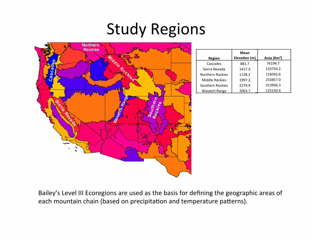
Study Regions

Bailey’s Level III Ecoregions are used as the basis for defining the geographic areas of each mountain chain (based on precipita,on and temperature pagerns).

Region Mean

ElevaOon (m) Cascades 881.7

Sierra Nevada 1417.3 Northern Rockies 1128.2 Middle Rockies 1997.2 Southern Rockies 2279.9 Wasatch Range 2063.7

Area (Km2) 76194.7 133754.2 116043.6 253857.0 313946.3 125150.4

Since high resolu,on is important, where and how do we get accurate, high resolu,on data?

Several choices (based on literature review): 1)  Global Climate Models

2)  Regional Models (NARR/NARCCAP) 3)  Sta,s,cally downscaled regionally model data

4)  Satellite 5)  Observa,ons alone – fine for local studies, but can’t generalize observa,ons without some sort of adjustments (or a lot of adjustments)

6)  Knowledge Based Downscaling – not just a basic interpolaOon technique (such as kriging or inverse weighOng), but a knowledge based algorithm

PRISM (Parameter-‐elevaOon Regression on Independent Slopes Model)

•  Daly, Christopher et al. (2008) – Oregon State University

•  Monthly (1895 – 2011) •  4km or 800m resolu,on

How does PRISM work? PRISM uses a knowledge based system (KBS) which “injects knowledge into a climate mapping system”

Major Components

1)  Eleva,on 2)  Terrain Induced Climate Transi,ons (rain

shadow, topographic facets) 3)  Two Layer Atmosphere & Topographic Index

4)  Coastal Effects

Moving window Regression

Combined weight of a sta,on is:

W = f {Wd Wz Wc Wf Wp Wl Wt We}

-‐  Distance -‐  Eleva,on -‐  Clustering -‐  Topographic Facet

(orienta,on)

-‐  Coastal Proximity -‐  Ver,cal Layer (inversion) -‐  Topographic Index (cold air pooling) -‐  Effec,ve Terrain Height (orographic

profile)

Dominant PRISM KBS Components ElevaOon Topographic Index Inversion Layer

-‐18° -‐13°

-‐18°C

Gunnison

One example of PRISM’s algorithm detec,ng/reproducing inversion layer -‐ (‘banana belt’) of CO Rockies

Source: PRISM Overview (5-‐8-‐08)

Inversions (1971-‐00 January Minimum Temperature Central Colorado)

Sta,s,cal Methods 1)  Linear Regression – on mean temperature trends

for each ecoregion (°C/yr) and eleva,onal trend analysis (°C/yr/km)

2)  K-‐means cluster analysis – as a complement to linear regression, used to determine eleva,onal trends for en,re western U.S. (°C/yr/km)

3)  Seasonal Trend Analysis – on mean monthly temperatures for each ecoregion; this is a general harmonic regression analysis to pick out general seasonal temperature/,ming trends

Digital ElevaOon Model and ElevaOonal Temperature Trend Regions

White areas indicate buffered ecoregions for eleva,onal trend analysis. These are buffered to include more sta,ons and a greater eleva,on range.

Results

-‐ Generally, trend maps don’t clearly outline mountain ranges -‐ This is probably good, since it’s an indica,on that PRISM isn’t biased toward using eleva,on as a forcing for temperatures or temperature trends

U.S. Tmin 1941 – 1970 Trends (C/yr) U.S. Tmin 1971 – 2000 Trends (C/yr)

Why 30 Year Running Means?

-‐0.15

-‐0.10

-‐0.05

0.00

0.05

0.10

0.15

0.20

1895

1902

1909

1916

1923

1930

1937

1944

1951

1958

1965

1972

1979

1986

1993

2000

Tempe

rature Trend

(C/year)

Sierra Nevada Minimum Temperature

10 Year

20 Year

30 Year

40 Year

50 Year

-‐0.10

-‐0.05

0.00

0.05

0.10

0.15

0.20

0.25

0.30

1895

1902

1909

1916

1923

1930

1937

1944

1951

1958

1965

1972

1979

1986

1993

2000

Tempe

rature Trend

(C/year)

Sierra Nevada Maximum Temperature

10 Year

20 Year

30 Year

40 Year

50 Year

Mean Temperature Trends -‐ Cascades

-‐0.08

-‐0.06

-‐0.04

-‐0.02

0

0.02

0.04

0.06

0.08

0.1 1895

1900

1905

1910

1915

1920

1925

1930

1935

1940

1945

1950

1955

1960

1965

1970

1975

1980

Tempe

rature Trend

(C/year)

Cascades 30 Year Running Mean Minimum Temperature Trend

Winter

Spring

Summer

Fall

-‐0.08

-‐0.06

-‐0.04

-‐0.02

0

0.02

0.04

0.06

0.08

0.1

1895

1900

1905

1910

1915

1920

1925

1930

1935

1940

1945

1950

1955

1960

1965

1970

1975

1980

Tempe

rature Trend

(C/year)

Cascades 30 Year Running Mean Maximum Temperature Trend

Winter

Spring

Summer

Fall

-‐ Cascades experience rela,vely ligle varia,on in mean temperature trends -‐ Maximum trends are more variable than minimum trends

-‐  Spring trends tend to peak before by 1965 and then decrease

-‐  Summer maximum trends are rising the fastest, perhaps due to the lack summer precipita,on

Mean Temperature Trends – Southern Rockies

-‐0.08

-‐0.06

-‐0.04

-‐0.02

0

0.02

0.04

0.06

0.08

1895

1900

1905

1910

1915

1920

1925

1930

1935

1940

1945

1950

1955

1960

1965

1970

1975

1980

Tempe

rature Trend

(C/year)

Southern Rockies 30 Year Running Mean Maximum Temperature Trend

Winter

Spring

Summer

Fall

-‐0.08

-‐0.06

-‐0.04

-‐0.02

0

0.02

0.04

0.06

0.08 1895

1900

1905

1910

1915

1920

1925

1930

1935

1940

1945

1950

1955

1960

1965

1970

1975

1980

Tempe

rature Trend

(C/year)

Southern Rockies 30 Year Running Mean Minimum Temperature Trend

Winter

Spring

Summer

Fall

-‐ Similar to the Cascades, minimum trends for the SR are less variable overall. But, they experience a larger, recent trend.

-‐ Maximum trends experience a large cyclical pagern, with a peak in the 1910’s and another recent peak.

-‐ Spring trends are earlier for minimum trends, but for maximum trends they are only larger.

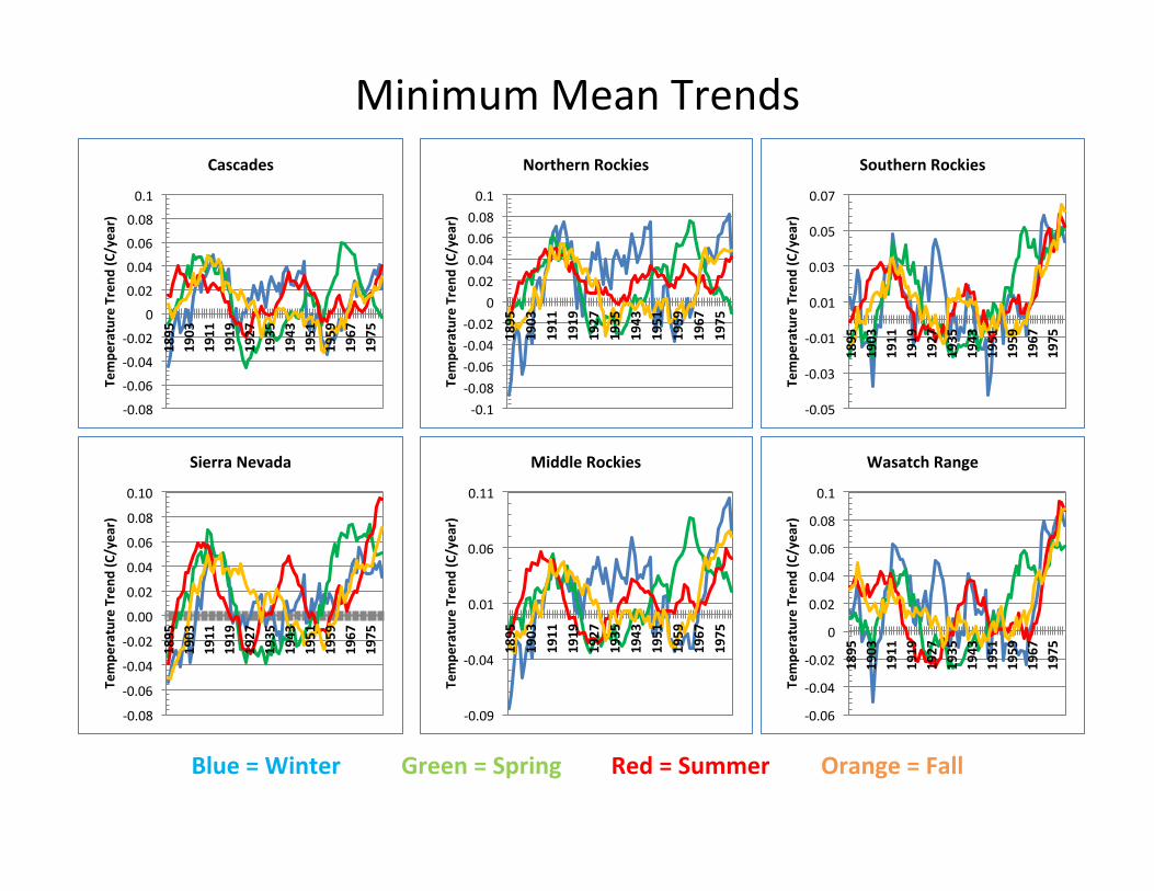
Minimum Mean Trends

-‐0.08

-‐0.06

-‐0.04

-‐0.02

0

0.02

0.04

0.06

0.08

0.1

1895

1903

1911

1919

1927

1935

1943

1951

1959

1967

1975

Tempe

rature Trend

(C/year)

Cascades

-‐0.08

-‐0.06

-‐0.04

-‐0.02

0.00

0.02

0.04

0.06

0.08

0.10

1895

1903

1911

1919

1927

1935

1943

1951

1959

1967

1975

Tempe

rature Trend

(C/year)

Sierra Nevada

-‐0.1 -‐0.08 -‐0.06 -‐0.04 -‐0.02

0 0.02 0.04 0.06 0.08 0.1

1895

1903

1911

1919

1927

1935

1943

1951

1959

1967

1975

Tempe

rature Trend

(C/year)

Northern Rockies

-‐0.09

-‐0.04

0.01

0.06

0.11 1895

1903

1911

1919

1927

1935

1943

1951

1959

1967

1975

Tempe

rature Trend

(C/year)

Middle Rockies

-‐0.05

-‐0.03

-‐0.01

0.01

0.03

0.05

0.07

1895

1903

1911

1919

1927

1935

1943

1951

1959

1967

1975

Tempe

rature Trend

(C/year)

Southern Rockies

-‐0.06

-‐0.04

-‐0.02

0

0.02

0.04

0.06

0.08

0.1

1895

1903

1911

1919

1927

1935

1943

1951

1959

1967

1975

Tempe

rature Trend

(C/year)

Wasatch Range

Blue = Winter Green = Spring Red = Summer Orange = Fall

Maximum Mean Trends

-‐0.06

-‐0.04

-‐0.02

0

0.02

0.04

0.06

0.08

0.1

0.12

1895

1904

1913

1922

1931

1940

1949

1958

1967

1976

Tempe

rature tren

d (C/year)

Wasatch

-‐0.08

-‐0.06

-‐0.04

-‐0.02

0

0.02

0.04

0.06

0.08

1895

1904

1913

1922

1931

1940

1949

1958

1967

1976

Tempe

rature Trend

(C/year)

Southern Rockies

-‐0.09

-‐0.04

0.01

0.06

0.11

1895

1903

1911

1919

1927

1935

1943

1951

1959

1967

1975

Tempe

rature Trend

(C/year)

Middle Rockies

-‐0.1 -‐0.08 -‐0.06 -‐0.04 -‐0.02

0 0.02 0.04 0.06 0.08 0.1

1895

1903

1911

1919

1927

1935

1943

1951

1959

1967

1975

Tempe

rature Trend

(C/year)

Northern Rockies

-‐0.08

-‐0.06

-‐0.04

-‐0.02

0

0.02

0.04

0.06

0.08

0.1

1895

1903

1911

1919

1927

1935

1943

1951

1959

1967

1975

Tempe

rature Trend

(C/year)

Sierra Nevada

-‐0.08

-‐0.06

-‐0.04

-‐0.02

0

0.02

0.04

0.06

0.08

0.1

1895

1903

1911

1919

1927

1935

1943

1951

1959

1967

1975

Tempe

rature Trend

(C/year)

Cascades


Eleva,onal Temperature Trends -‐ Clustering

What is K-‐Means Clustering? -‐ An itera,ve data mining technique that divides a set of

observa,ons into a specific number of groups (clusters) where the intra-‐cluster variance is minimized and the inter-‐cluster variance

is maximized

-‐  Performed for both minimum and maximum temperature trends for two periods, 1941 – 1970 and 1971 – 2000 for the en,re

western U.S. (west of 105°W)

Four Variable Results – each season separately

-‐0.0020

-‐0.0015

-‐0.0010

-‐0.0005

0.0000

0.0005

0.0010

0.0015 0

500

1000

1500

2000

2500

3000

3500

Centroid Tem

perature Trend

(C/yr)

Mean Cluster ElevaOon

Winter 1941 – 1970 (both +)

-‐0.0020

-‐0.0015

-‐0.0010

-‐0.0005

0.0000

0.0005

0.0010

0.0015

0

500

1000

1500

2000

2500

3000

3500

Centroid Tem

perature Trend

(C/yr)


Spring 1941 – 1970 (both -‐)

-‐0.0015

-‐0.0010

-‐0.0005

0.0000

0.0005

0.0010

0.0015

0.0020

0

500

1000

1500

2000

2500

Centroid Tem

perature Trend

(C/yr)


Winter 1971 – 2000 (Tmax -‐)

-‐0.0015

-‐0.0010

-‐0.0005

0.0000

0.0005

0.0010

0.0015

0.0020

0

500

1000

1500

2000

2500

Centroid Tem

perature Trend

(C/yr)


Spring 1971 – 2000 (both +)

Eleva,onal Temperature Trends – Linear Regression

-‐0.04

-‐0.03

-‐0.02

-‐0.01

0

0.01

0.02

0.03

0.04

1895

1899

1903

1907

1911

1915

1919

1923

1927

1931

1935

1939

1943

1947

1951

1955

1959

1963

1967

1971

1975

1979

Tempe

rature Trend

(C/yr/km

)

Cascades Maximum ElevaOonal Trends

-‐0.04

-‐0.03

-‐0.02

-‐0.01

0

0.01

0.02

0.03

0.04

1895

1899

1903

1907

1911

1915

1919

1923

1927

1931

1935

1939

1943

1947

1951

1955

1959

1963

1967

1971

1975

1979

ElevaO

onal Tem

perature Trend

(C/yr/

km)

Cascades Minimum ElevaOonal Trend

Maximum trends show a general decrease in magnitude with ,me. Minimum trends show a cyclical pagern, and have recently converged.

Eleva,onal Temperature Trends – Linear Regression

-‐0.03

-‐0.02

-‐0.01

0

0.01

0.02

0.03

0.04

0.05

0.06 1895

1899

1903

1907

1911

1915

1919

1923

1927

1931

1935

1939

1943

1947

1951

1955

1959

1963

1967

1971

1975

1979

ElevaO

onal Tem

perature Trend

(C/yr/

km)

Middle Rockies Maximum ElevaOonal Trend

-‐0.03

-‐0.02

-‐0.01

0

0.01

0.02

0.03

0.04

0.05

0.06

1895

1899

1903

1907

1911

1915

1919

1923

1927

1931

1935

1939

1943

1947

1951

1955

1959

1963

1967

1971

1975

1979

ElevaO

onal Tem

perature Trend

(C/yr/

km)

Middle Rockies Minimum ElevaOonal Trend

Both minimum and maximum trends show large increases aQer 1960. Maximum spring eleva,onal temperature trends show the greatest difference with eleva,on

Minimum Eleva,onal Temperature Trends

-‐0.04

-‐0.03

-‐0.02

-‐0.01

0

0.01

0.02

0.03

0.04 1895

1903

1911

1919

1927

1935

1943

1951

1959

1967

1975

ElevaO

onal Tem

perature Trend

(C/yr/

km)

Cascades

-‐0.03

-‐0.02

-‐0.01

0

0.01

0.02

0.03

0.04

0.05

0.06 1895

1903

1911

1919

1927

1935

1943

1951

1959

1967

1975

ElevaO

onal Tem

perature Trend

(C/yr/

km)

Middle Rockies

-‐0.03

-‐0.02

-‐0.01

0

0.01

0.02

0.03

1895

1903

1911

1919

1927

1935

1943

1951

1959

1967

1975

ElevaO

onal Tem

perature Trend

(C/yr/

km)

Sierra Nevada

-‐0.06

-‐0.04

-‐0.02

0

0.02

0.04

0.06

1895

1903

1911

1919

1927

1935

1943

1951

1959

1967

1975

ElevaO

onal Tem

perature Trend

(C/yr/

km)

Northern Rockies

-‐0.04

-‐0.03

-‐0.02

-‐0.01

0

0.01

0.02

0.03

0.04

0.05

1895

1903

1911

1919

1927

1935

1943

1951

1959

1967

1975

ElevaO

onal Tem

perature Trend

(C/yr/

km)

Southern Rockies

-‐0.03

-‐0.02

-‐0.01

0

0.01

0.02

0.03

0.04

0.05

0.06

0.07

1895

1903

1911

1919

1927

1935

1943

1951

1959

1967

1975

ElevaO

onal Tem

perature Trend

(C/yr/

km)

Wasatch


Maximum Eleva,onal Temperature Trends

-‐0.04

-‐0.03

-‐0.02

-‐0.01

0

0.01

0.02

0.03

0.04 1895

1903

1911

1919

1927

1935

1943

1951

1959

1967

1975

Tempe

rature Trend

(C/yr/km

)

Cascades

-‐0.03

-‐0.02

-‐0.01

0

0.01

0.02

0.03

0.04

0.05

0.06

1895

1903

1911

1919

1927

1935

1943

1951

1959

1967

1975

ElevaO

onal Tem

perature Trend

(C/yr/

km)

Middle Rockies

-‐0.03

-‐0.02

-‐0.01

0

0.01

0.02

0.03

1895

1904

1913

1922

1931

1940

1949

1958

1967

1976

ElevaO

onal Tem

perature Trend

(C/yr/

km)

Sierra Nevada

-‐0.06

-‐0.04

-‐0.02

0

0.02

0.04

0.06

1895

1903

1911

1919

1927

1935

1943

1951

1959

1967

1975

ElevaO

onal Tem

perature Trend

(C/yr/

km)

Northern Rockies)

-‐0.04

-‐0.03

-‐0.02

-‐0.01

0

0.01

0.02

0.03

0.04

0.05

1895

1903

1911

1919

1927

1935

1943

1951

1959

1967

1975

ElevaO

onal Tem

perature Trend

(C/yr/

km)

Southern Rockies

-‐0.03

-‐0.01

0.01

0.03

0.05

0.07

1895

1903

1911

1919

1927

1935

1943

1951

1959

1967

1975

ElevaO

onal Tem

perature Trend

(C/yr/

km)

Wasatch


Results – Seasonal Trend Analysis Developed by Ronald Eastman of Clark Labs , Clark University, MA (Eastman, et al. 2009)

What is Seasonal Trend Analysis (STA)?

Uses harmonic regression to determine general seasonal curves (,ming and temperature magnitude)

Designed to ignore sub-‐annual varia,ons and to be robust to short

term variability up to 29% the length of the ,me series

Seasonal Trend Analysis – cont’d

•  1942 – 1971 and 1971 – 2000 •  Based on actual temperatures, not trends

•  Provides a good snapshot of the shorter term seasonal trends or varia,ons

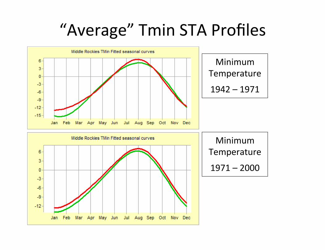
“Average” Tmin STA Profiles

Minimum Temperature

1942 – 1971

Minimum Temperature

1971 – 2000

“Average” Tmax STA Profiles

Maximum Temperature

1942 – 1971

Maximum Temperature

1971 – 2000

Sierra Nevada -‐ STA

Minimum Temperature

1942 – 1971

Minimum Temperature

1971 – 2000

Discussion – Literature Comparison •  Cluster analysis shows strong posi,ve spring temperature trend rela,onship with eleva,on – Is this in contrast to Pepin and Lundquist (2008)?

•  Conklin and Osborne-‐Gowey (2010 MTN CLIM conference) used 800m data to study Sierra Nevada temperature trends. Do our analyses agree?

Summary – temperature trends •  Recent mean temperature trends are posi,ve for fall, summer, winter

•  Mean spring trends peaked about 1960 in most regions and then began a decline

•  Mean maximum temperature trends tend to be more variable than minimum trends

•  Eleva,onal trends follow similar pagerns as mean trends, but spring trends are the strongest (no ,ming difference, however)

Why might spring trends be the strongest or peak earlier than the

other seasons? Reduced winter snowpack

Snow can melt earlier

Spring temperatures can rise faster

One more ques,on…

•  Recall –  Cascades & Sierra Nevada highly variable eleva,onal trends throughout ,me period

–  But, Rockies and Wasatch generally experience rela,vely flat eleva,onal trends through 1960, and then experience rapid increases

Why? Cascades and Sierra Nevada – highly mari,me

influenced, so the more con,nental a range is, the less effect ENSO/other ocean variability has.

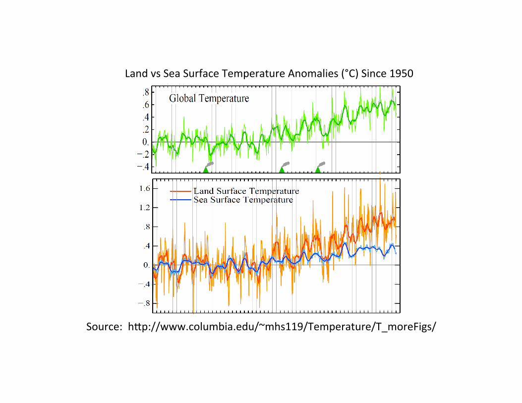
Source: hgp://www.columbia.edu/~mhs119/Temperature/T_moreFigs/

Land vs Sea Surface Temperature Anomalies (°C) Since 1950

Future Work •  Use 800m data for analysis

•  Cluster individual ecoregions •  Do STA by eleva,on •  Do a snow cover/temp trend analysis •  Future data sets look very promising -‐ several projects have or are installing very high density observa,on networks (“massive air and stream temperature sensor networks”) across the western U.S.

Acknowledgements •  Ankur Desai •  Steve Vavrus, CDC •  Dan Vimont and Chris Kucharik •  Bjorn Brooks •  Sam Batzli •  Fellow graduate students •  UW Graduate School and DOE Funding •  My family

References Beniston, M., Diaz,H.F. and Bradley, R.S. (1997). Clima,c change at high

eleva,on sites: An overview. Clima)c Change, Vol. 36, 233–252.

Daly, Christopher et al. (2008). Physiographically sensi,ve mapping of climatological temperature and precipita,on across the conterminous United States. Interna)onal Journal of Climatology, DOI: 10.1002.

Diaz, Henry F. and Bradley, Raymond S. (1997). Temperature varia,ons during the last century at high eleva,on sites. Clima)c Change, Vol. 36, 253 – 279.

Pepin, Nick and Lundquist, Jessica. Temperature trends in North American mountains: a global context. Poster. Presented at CIRMOUNT, Silverton, CO, June 9 – 12, 2008.

One issue: Surface temperature trends vs. free air temperature trends

•  Surface temperatures – affected by surface complexi,es •  Free air temperatures – temps of atmosphere not directly in

contact with/affected by surface

•  Complex issue and extremely poorly understood, as it deals with trends in lapse rates.

•  Measured to be significantly different in some cases (the opposite, in fact). Interac,on with the surface may be changing the surface trend (as indicated by the greatest warming located near the 0°C isotherm – snow/ice feedback).

•  Mountain summits and loca,ons where air can move freely experience a much more consistent, linear trend. Pepin and Lundquist (2008) state that this doesn’t necessarily mean mountains are more sensi,ve to poten,al climate change, but that they are taking a beger record of the free air temperature.

Vuille and Bradley (2000), Pepin and Losloben (2002), and Gaffen et al. (2000).

“Geospa,al Climatology” •  A rela,vely new field which studies the effect of physiographic features on climate

Some (RelaOvely) Specific Factors 1)  Solar RadiaOon – varying exposures, facet direc,ons, slope angles, sunlight totals, etc.

2)  SynopOc pajern – cloud cover, overall wind speed/direc,on, precipita,on, humidity, etc. 3)  Land Cover – urban, forest, grassland, desert, lake/stream, glacier, etc. and changes in land

cover through space – (creates certain wind pagerns when combined with other two factors that further influence temperature pagerns)

Why should we care about such high resoluOon pajerns? -‐  Ecological/biological gradients mirror the high climatological

gradients (and resul,ng hydrological gradients) One (of countless) really cool example: The larvae of the black, basking caterpillar grow faster on

a sun facing, warm slope, and emerge as a bugerfly up to 5 weeks faster! (Weiss, et al. 1988)

Since high resolu,on is important, where and how do we get accurate, high resolu,on data?

Several choices (based on literature review): 1)  Global Climate Models – very low resolu,on, Pepin and Lundquist (2008)

indicate they produce too strong a warming feedback at the 0°C isotherm 2)  Regional Models (NARR/NARCCAP)-‐ a lot beger, but a 32 or 50 km

resolu,on is s,ll much too low 3)  Sta,s,cally downscaled regionally model data – may be good, but covers

rela,vely short ,me periods and small areas (10 – 12 km resolu,on ok, but not great)

4)  Satellite – may be good, but requires processing/interpreta,on of an enormous amount of data, covers a rela,vely short ,me period, and some

of this data has never been looked at or processed 5)  Observa,ons alone – fine for local studies, but can’t generalize observa,ons without some sort of adjustments (or a lot of adjustments)

6)  Downscaling – not just a basic interpolaOon technique (such as kriging or inverse weighOng), but a knowledge based algorithm

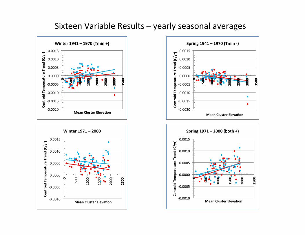
Sixteen Variable Results – yearly seasonal averages

-‐0.0020

-‐0.0015

-‐0.0010

-‐0.0005

0.0000

0.0005

0.0010

0.0015

0

500

1000

1500

2000

2500

3000

3500

Centroid Tem

perature Trend

(C/yr)


Winter 1941 – 1970 (Tmin +)

-‐0.0020

-‐0.0015

-‐0.0010

-‐0.0005

0.0000

0.0005

0.0010

0.0015

0

500

1000

1500

2000

2500

3000

3500

Centroid Tem

perature Trend

(C/yr)


Spring 1941 – 1970 (Tmin -‐)

-‐0.0010

-‐0.0005

0.0000

0.0005

0.0010

0.0015

0

500

1000

1500

2000

2500

Centroid Tem

perature Trend

(C/yr)


Winter 1971 – 2000

-‐0.0010

-‐0.0005

0.0000

0.0005

0.0010

0.0015

0

500

1000

1500

2000

2500

Centroid Tem

perature Trend

(C/yr)


Spring 1971 – 2000 (both +)

Despite these changes….

•  Mountainous regions have been poorly studied, in general (climate, ecology, etc.)

But Why? •  Remoteness means generally sparse popula,on, so neglected

since deemed ‘less important’ •  Remoteness also means physical access for installa,on and

maintenance of monitoring equipment is difficult •  High complexity of terrain means one sta,on represents only

a small por,on of region/mountain chain •  Making standard weather observa,ons (or others) is difficult

across such a large por,on of world, due to everything from different cultural, poli,cal, and even scien,fic standards/goals

ruben$behnke$ advisor: ankur$desai$ - webhome <...

Documents