rstudio ide cheat sheet open source server...
TRANSCRIPT
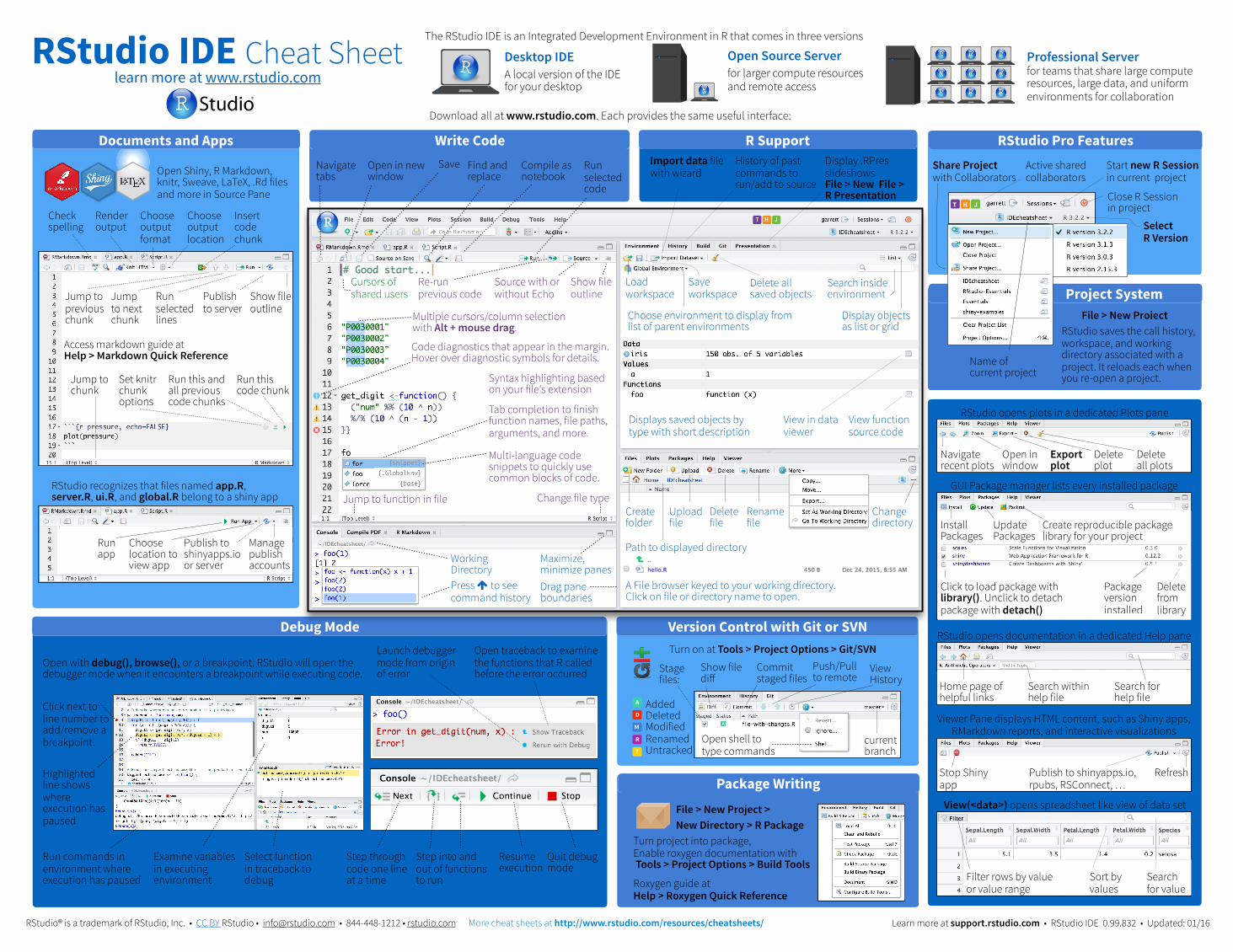
Documents and Apps
Project System
Write Code R Support RStudio Pro Features
Debug Mode Version Control with Git or SVN
Package Writing
Project System
Write Code R Support RStudio Pro Features
Debug Mode Version Control with Git or SVN
Package Writing
Turn project into package, Enable roxygen documentation with Tools > Project Options > Build Tools
Roxygen guide at Help > Roxygen Quick Reference
File > New Project > New Directory > R Package
learn more at www.rstudio.com
The RStudio IDE is an Integrated Development Environment in R that comes in three versions
Desktop IDE A local version of the IDE for your desktop
Open Source Server for larger compute resources and remote access
Professional Server for teams that share large compute resources, large data, and uniform environments for collaboration
Download all at www.rstudio.com. Each provides the same useful interface:
Share Project with Collaborators
Active shared collaborators
Select R Version
Start new R Session in current project
Close R Session in project JHT
RStudio saves the call history, workspace, and working directory associated with a project. It reloads each when you re-open a project.
Name of current project
View(<data>) opens spreadsheet like view of data set
Sort by values
Filter rows by value or value range
Search for value
Viewer Pane displays HTML content, such as Shiny apps, RMarkdown reports, and interactive visualizations
Stop Shiny app
Publish to shinyapps.io, rpubs, RSConnect, …
Refresh
RStudio opens documentation in a dedicated Help pane
Home page of helpful links
Search within help file
Search for help file
GUI Package manager lists every installed package
Click to load package with library(). Unclick to detach package with detach()
Delete from library
Install Packages
Update Packages
Create reproducible package library for your project
RStudio opens plots in a dedicated Plots pane
Navigate recent plots
Open in window
Export plot
Delete plot
Delete all plots
Package version installed
Examine variables in executing environment
Open with debug(), browse(), or a breakpoint. RStudio will open the debugger mode when it encounters a breakpoint while executing code.
Open traceback to examine the functions that R called before the error occurred
Launch debugger mode from origin of error
Click next to line number to add/remove a breakpoint.
Select function in traceback to debug
Highlighted line shows where execution has paused
Run commands in environment where execution has paused
Step through code one line at a time
Step into and out of functions to run
Resume execution
Quit debug mode
Open Shiny, R Markdown, knitr, Sweave, LaTeX, .Rd files and more in Source Pane
Check spelling
Render output
Choose output format
Choose output location
Insert code chunk
Jump to previous chunk
Jump to next chunk
Run selected lines
Publish to server
Show file outline
Set knitr chunk options
Run this and all previous code chunks
Run this code chunk
Jump to chunk
RStudio recognizes that files named app.R, server.R, ui.R, and global.R belong to a shiny app
Run app
Choose location to view app
Publish to shinyapps.io or server
Manage publish accounts
Access markdown guide at Help > Markdown Quick Reference
RStudio IDE Cheat Sheet
RStudio® is a trademark of RStudio, Inc. • CC BY RStudio • [email protected] • 844-448-1212 • rstudio.com Learn more at support.rstudio.com • RStudio IDE 0.99.832 • Updated: 01/16More cheat sheets at http://www.rstudio.com/resources/cheatsheets/
Stage files:
Show file diff
Commit staged files
Push/Pull to remote
View History
current branch
• Added • Deleted • Modified • Renamed • Untracked
Turn on at Tools > Project Options > Git/SVN
Open shell to type commands
A
D
M
R
?
Search inside environment
Syntax highlighting based on your file's extension
Code diagnostics that appear in the margin. Hover over diagnostic symbols for details.
Tab completion to finish function names, file paths, arguments, and more.
Multi-language code snippets to quickly use common blocks of code.
Open in new window
Save Find and replace
Compile as notebook
Run selected code
Re-run previous code
Source with or without Echo
Show file outline
Jump to function in file Change file type
Navigate tabs
A File browser keyed to your working directory. Click on file or directory name to open.
Path to displayed directory
Upload file
Create folder
Delete file
Rename file
Change directory
Displays saved objects by type with short description
View function source code
View in data viewer
Load workspace
Save workspace
Import data file with wizard
Delete all saved objects
Display objects as list or grid
Choose environment to display from list of parent environments
History of past commands to run/add to source
Display .RPres slideshows File > New File > R Presentation
Working Directory
Maximize, minimize panesDrag pane boundaries
JHT
Cursors of shared users
File > New Project
Press ! to see command history
Multiple cursors/column selection with Alt + mouse drag.
Documents and Apps
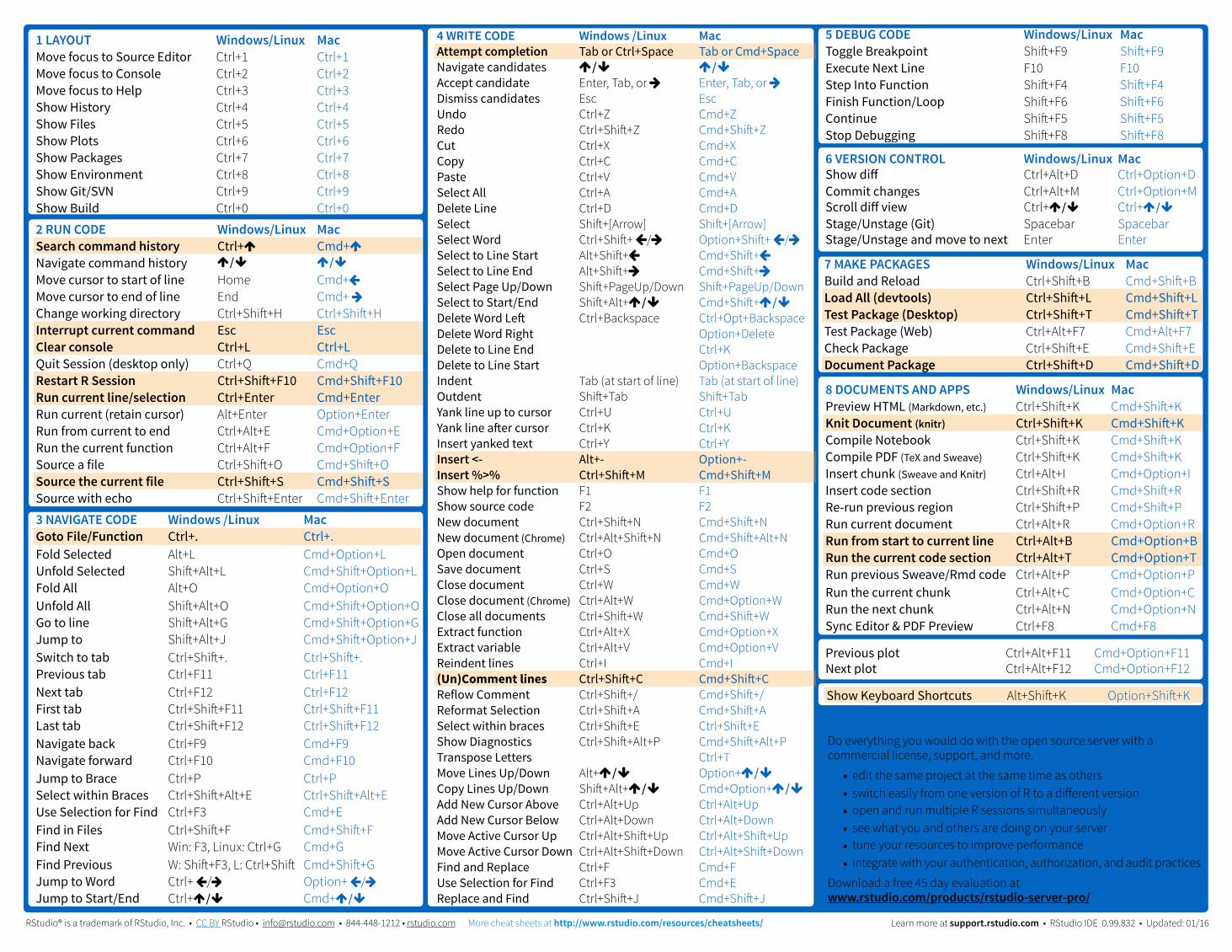
1 LAYOUT Windows/Linux MacMove focus to Source Editor Ctrl+1 Ctrl+1Move focus to Console Ctrl+2 Ctrl+2Move focus to Help Ctrl+3 Ctrl+3Show History Ctrl+4 Ctrl+4Show Files Ctrl+5 Ctrl+5Show Plots Ctrl+6 Ctrl+6Show Packages Ctrl+7 Ctrl+7Show Environment Ctrl+8 Ctrl+8Show Git/SVN Ctrl+9 Ctrl+9Show Build Ctrl+0 Ctrl+0
4 WRITE CODE Windows /Linux MacAttempt completion Tab or Ctrl+Space Tab or Cmd+SpaceNavigate candidates !/" !/"Accept candidate Enter, Tab, or # Enter, Tab, or #Dismiss candidates Esc EscUndo Ctrl+Z Cmd+ZRedo Ctrl+Shift+Z Cmd+Shift+ZCut Ctrl+X Cmd+XCopy Ctrl+C Cmd+CPaste Ctrl+V Cmd+VSelect All Ctrl+A Cmd+ADelete Line Ctrl+D Cmd+DSelect Shift+[Arrow] Shift+[Arrow]Select Word Ctrl+Shift+ $/# Option+Shift+ $/#Select to Line Start Alt+Shift+$ Cmd+Shift+$Select to Line End Alt+Shift+# Cmd+Shift+#Select Page Up/Down Shift+PageUp/Down Shift+PageUp/DownSelect to Start/End Shift+Alt+!/" Cmd+Shift+!/"Delete Word Left Ctrl+Backspace Ctrl+Opt+BackspaceDelete Word Right Option+DeleteDelete to Line End Ctrl+KDelete to Line Start Option+BackspaceIndent Tab (at start of line) Tab (at start of line)Outdent Shift+Tab Shift+TabYank line up to cursor Ctrl+U Ctrl+UYank line after cursor Ctrl+K Ctrl+KInsert yanked text Ctrl+Y Ctrl+YInsert <- Alt+- Option+-Insert %>% Ctrl+Shift+M Cmd+Shift+MShow help for function F1 F1Show source code unction
F2 F2New document Ctrl+Shift+N Cmd+Shift+NNew document (Chrome) Ctrl+Alt+Shift+N Cmd+Shift+Alt+NOpen document Ctrl+O Cmd+OSave document Ctrl+S Cmd+SClose document Ctrl+W Cmd+WClose document (Chrome) Ctrl+Alt+W Cmd+Option+WClose all documents Ctrl+Shift+W Cmd+Shift+WExtract function Ctrl+Alt+X Cmd+Option+XExtract variable Ctrl+Alt+V Cmd+Option+VReindent lines Ctrl+I Cmd+I(Un)Comment lines Ctrl+Shift+C Cmd+Shift+CReflow Comment Ctrl+Shift+/ Cmd+Shift+/Reformat Selection Ctrl+Shift+A Cmd+Shift+ASelect within braces Ctrl+Shift+E Ctrl+Shift+EShow Diagnostics Ctrl+Shift+Alt+P Cmd+Shift+Alt+PTranspose Letters Ctrl+TMove Lines Up/Down Alt+!/" Option+!/"Copy Lines Up/Down Shift+Alt+!/" Cmd+Option+!/"Add New Cursor Above Ctrl+Alt+Up Ctrl+Alt+UpAdd New Cursor Below Ctrl+Alt+Down Ctrl+Alt+DownMove Active Cursor Up Ctrl+Alt+Shift+Up Ctrl+Alt+Shift+UpMove Active Cursor Down Ctrl+Alt+Shift+Down Ctrl+Alt+Shift+DownFind and Replace Ctrl+F Cmd+FUse Selection for Find Ctrl+F3 Cmd+EReplace and Find Ctrl+Shift+J Cmd+Shift+J
2 RUN CODE Windows/Linux MacSearch command history Ctrl+! Cmd+!Navigate command history !/" !/"Move cursor to start of line Home Cmd+$Move cursor to end of line End Cmd+ #Change working directory Ctrl+Shift+H Ctrl+Shift+HInterrupt current command Esc EscClear console Ctrl+L Ctrl+LQuit Session (desktop only) Ctrl+Q Cmd+QRestart R Session Ctrl+Shift+F10 Cmd+Shift+F10Run current line/selection Ctrl+Enter Cmd+EnterRun current (retain cursor) Alt+Enter Option+EnterRun from current to end Ctrl+Alt+E Cmd+Option+ERun the current function definition
Ctrl+Alt+F Cmd+Option+FSource a file Ctrl+Shift+O Cmd+Shift+OSource the current file Ctrl+Shift+S Cmd+Shift+SSource with echo Ctrl+Shift+Enter Cmd+Shift+Enter
RStudio® is a trademark of RStudio, Inc. • CC BY RStudio • [email protected] • 844-448-1212 • rstudio.com Learn more at support.rstudio.com • RStudio IDE 0.99.832 • Updated: 01/16More cheat sheets at http://www.rstudio.com/resources/cheatsheets/
3 NAVIGATE CODE Windows /Linux MacGoto File/Function Ctrl+. Ctrl+.Fold Selected Alt+L Cmd+Option+LUnfold Selected Shift+Alt+L Cmd+Shift+Option+LFold All Alt+O Cmd+Option+OUnfold All Shift+Alt+O Cmd+Shift+Option+OGo to line Shift+Alt+G Cmd+Shift+Option+GJump to Shift+Alt+J Cmd+Shift+Option+JSwitch to tab Ctrl+Shift+. Ctrl+Shift+.Previous tab Ctrl+F11 Ctrl+F11Next tab Ctrl+F12 Ctrl+F12First tab Ctrl+Shift+F11 Ctrl+Shift+F11Last tab Ctrl+Shift+F12 Ctrl+Shift+F12Navigate back Ctrl+F9 Cmd+F9Navigate forward Ctrl+F10 Cmd+F10Jump to Brace Ctrl+P Ctrl+PSelect within Braces Ctrl+Shift+Alt+E Ctrl+Shift+Alt+EUse Selection for Find Ctrl+F3 Cmd+EFind in Files Ctrl+Shift+F Cmd+Shift+FFind Next Win: F3, Linux: Ctrl+G Cmd+GFind Previous W: Shift+F3, L: Ctrl+Shift
+GCmd+Shift+G
Jump to Word Ctrl+ $/# Option+ $/#Jump to Start/End Ctrl+!/" Cmd+!/"
5 DEBUG CODE Windows/Linux MacToggle Breakpoint Shift+F9 Shift+F9Execute Next Line F10 F10Step Into Function Shift+F4 Shift+F4Finish Function/Loop Shift+F6 Shift+F6Continue Shift+F5 Shift+F5Stop Debugging Shift+F8 Shift+F8
6 VERSION CONTROL Windows/Linux MacShow diff Ctrl+Alt+D Ctrl+Option+DCommit changes Ctrl+Alt+M Ctrl+Option+MScroll diff view Ctrl+!/" Ctrl+!/"Stage/Unstage (Git) Spacebar SpacebarStage/Unstage and move to next Enter Enter
7 MAKE PACKAGES Windows/Linux MacBuild and Reload Ctrl+Shift+B Cmd+Shift+BLoad All (devtools) Ctrl+Shift+L Cmd+Shift+LTest Package (Desktop) Ctrl+Shift+T Cmd+Shift+TTest Package (Web) Ctrl+Alt+F7 Cmd+Alt+F7Check Package Ctrl+Shift+E Cmd+Shift+EDocument Package Ctrl+Shift+D Cmd+Shift+D
8 DOCUMENTS AND APPS Windows/Linux MacPreview HTML (Markdown, etc.) Ctrl+Shift+K Cmd+Shift+KKnit Document (knitr) Ctrl+Shift+K Cmd+Shift+KCompile Notebook Ctrl+Shift+K Cmd+Shift+KCompile PDF (TeX and Sweave) Ctrl+Shift+K Cmd+Shift+KInsert chunk (Sweave and Knitr) Ctrl+Alt+I Cmd+Option+IInsert code section Ctrl+Shift+R Cmd+Shift+RRe-run previous region Ctrl+Shift+P Cmd+Shift+PRun current document Ctrl+Alt+R Cmd+Option+RRun from start to current line Ctrl+Alt+B Cmd+Option+BRun the current code section Ctrl+Alt+T Cmd+Option+TRun previous Sweave/Rmd code Ctrl+Alt+P Cmd+Option+PRun the current chunk Ctrl+Alt+C Cmd+Option+CRun the next chunk Ctrl+Alt+N Cmd+Option+NSync Editor & PDF Preview Ctrl+F8 Cmd+F8
Previous plot Ctrl+Alt+F11 Cmd+Option+F11Next plot Ctrl+Alt+F12 Cmd+Option+F12
Show Keyboard Shortcuts Alt+Shift+K Option+Shift+K
Why RStudio Server Pro?Do everything you would do with the open source server with a commercial license, support, and more.
• edit the same project at the same time as others • switch easily from one version of R to a different version • open and run multiple R sessions simultaneously • see what you and others are doing on your server • tune your resources to improve performance • integrate with your authentication, authorization, and audit practices
Download a free 45 day evaluation at www.rstudio.com/products/rstudio-server-pro/
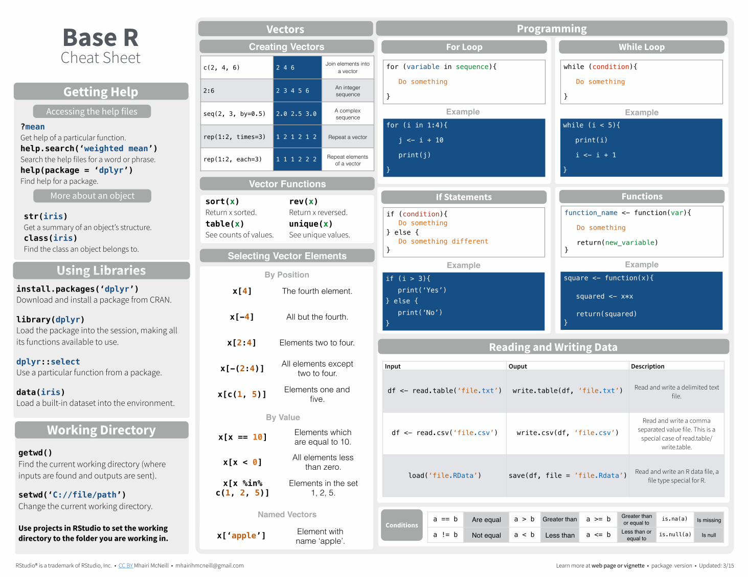
Base R Cheat Sheet
RStudio® is a trademark of RStudio, Inc. • CC BY Mhairi McNeill • [email protected] Learn more at web page or vignette • package version • Updated: 3/15
Input Ouput Description
df <- read.table(‘file.txt’) write.table(df, ‘file.txt’) Read and write a delimited text file.
df <- read.csv(‘file.csv’) write.csv(df, ‘file.csv’)
Read and write a comma separated value file. This is a
special case of read.table/write.table.
load(‘file.RData’) save(df, file = ’file.Rdata’) Read and write an R data file, a file type special for R.
?mean Get help of a particular function. help.search(‘weighted mean’) Search the help files for a word or phrase. help(package = ‘dplyr’) Find help for a package.
Getting HelpAccessing the help files
More about an object
str(iris) Get a summary of an object’s structure. class(iris) Find the class an object belongs to.
ProgrammingFor Loop
for (variable in sequence){
Do something
}
Examplefor (i in 1:4){
j <- i + 10
print(j)
}
While Loop
while (condition){
Do something
}
Examplewhile (i < 5){
print(i)
i <- i + 1
}
If Statements
if (condition){ Do something
} else { Do something different
}
Exampleif (i > 3){
print(‘Yes’) } else {
print(‘No’) }
Functionsfunction_name <- function(var){
Do something
return(new_variable) }
Examplesquare <- function(x){
squared <- x*x
return(squared) }
a == b Are equal a > b Greater than a >= b Greater than or equal to
is.na(a) Is missing
a != b Not equal a < b Less than a <= b Less than or equal to
is.null(a) Is null Conditions
Creating Vectors
c(2, 4, 6) 2 4 6 Join elements into a vector
2:6 2 3 4 5 6 An integer sequence
seq(2, 3, by=0.5) 2.0 2.5 3.0 A complex sequence
rep(1:2, times=3) 1 2 1 2 1 2 Repeat a vector
rep(1:2, each=3) 1 1 1 2 2 2 Repeat elements of a vector
Using Librariesinstall.packages(‘dplyr’) Download and install a package from CRAN.
library(dplyr) Load the package into the session, making all its functions available to use.
dplyr::select Use a particular function from a package.
data(iris) Load a built-in dataset into the environment.
Vectors
Selecting Vector Elements
x[4] The fourth element.
x[-4] All but the fourth.
x[2:4] Elements two to four.
x[-(2:4)] All elements except two to four.
x[c(1, 5)] Elements one and five.
x[x == 10] Elements which are equal to 10.
x[x < 0] All elements less than zero.
x[x %in% c(1, 2, 5)]
Elements in the set 1, 2, 5.
By Position
By Value
Named Vectors
x[‘apple’] Element with name ‘apple’.
Reading and Writing Data
Working Directorygetwd() Find the current working directory (where inputs are found and outputs are sent).
setwd(‘C://file/path’) Change the current working directory.
Use projects in RStudio to set the working directory to the folder you are working in.
Vector Functionssort(x) Return x sorted.
rev(x) Return x reversed.
table(x) See counts of values.
unique(x) See unique values.
RStudio® is a trademark of RStudio, Inc. • CC BY Mhairi McNeill • [email protected] • 844-448-1212 • rstudio.com Learn more at web page or vignette • package version • Updated: 3/15
Lists
Matrixes
Data Frames
Maths Functions
Types Strings
Factors
Statistics
Distributions
as.logical TRUE, FALSE, TRUE Boolean values (TRUE or FALSE).
as.numeric 1, 0, 1 Integers or floating point numbers.
as.character '1', '0', '1' Character strings. Generally preferred to factors.
as.factor'1', '0', '1', levels: '1', '0'
Character strings with preset levels. Needed for some
statistical models.
Converting between common data types in R. Can always go from a higher value in the table to a lower value.
> a <- 'apple' > a [1] 'apple'
The Environment
Variable Assignment
ls() List all variables in the environment.
rm(x) Remove x from the environment.
rm(list = ls()) Remove all variables from the environment.
You can use the environment panel in RStudio to browse variables in your environment.
factor(x) Turn a vector into a factor. Can set the levels of the factor and
the order.
m <- matrix(x, nrow = 3, ncol = 3) Create a matrix from x.
wwwwwwm[2, ] - Select a row
m[ , 1] - Select a column
m[2, 3] - Select an elementwwwwwwwwwwww
t(m) Transpose m %*% n
Matrix Multiplication solve(m, n)
Find x in: m * x = n
l <- list(x = 1:5, y = c('a', 'b')) A list is collection of elements which can be of different types.
l[[2]] l[1] l$x l['y']
Second element of l.
New list with only the first
element.
Element named x.
New list with only element
named y.
df <- data.frame(x = 1:3, y = c('a', 'b', 'c')) A special case of a list where all elements are the same length.
t.test(x, y) Preform a t-test for difference between
means.
pairwise.t.test Preform a t-test for
paired data.
log(x) Natural log. sum(x) Sum.
exp(x) Exponential. mean(x) Mean.
max(x) Largest element. median(x) Median.
min(x) Smallest element. quantile(x) Percentage quantiles.
round(x, n) Round to n decimal places.
rank(x) Rank of elements.
signif(x, n) Round to n significant figures.
var(x) The variance.
cor(x, y) Correlation. sd(x) The standard deviation.
x y
1 a
2 b
3 c
Matrix subsetting
df[2, ]
df[ , 2]
df[2, 2]
List subsetting
df$x df[[2]]
cbind - Bind columns.
rbind - Bind rows.
View(df) See the full data frame.
head(df) See the first 6 rows.
Understanding a data frame
nrow(df) Number of rows.
ncol(df) Number of columns.
dim(df) Number of columns and rows.
Plotting
Dates See the lubridate library.
Also see the ggplot2 library.
Also see the stringr library.
Also see the dplyr library.
plot(x) Values of x in
order.
plot(x, y) Values of x against y.
hist(x) Histogram of
x.
Random Variates
Density Function
Cumulative Distribution
Quantile
Normal rnorm dnorm pnorm qnorm
Poison rpois dpois ppois qpois
Binomial rbinom dbinom pbinom qbinom
Uniform runif dunif punif qunif
lm(x ~ y, data=df) Linear model.
glm(x ~ y, data=df) Generalised linear model.
summary Get more detailed information
out a model.
prop.test Test for a difference between
proportions.
aov Analysis of variance.
paste(x, y, sep = ' ') Join multiple vectors together.
paste(x, collapse = ' ') Join elements of a vector together.
grep(pattern, x) Find regular expression matches in x.
gsub(pattern, replace, x) Replace matches in x with a string.
toupper(x) Convert to uppercase.
tolower(x) Convert to lowercase.
nchar(x) Number of characters in a string.
cut(x, breaks = 4) Turn a numeric vector into a
factor but ‘cutting’ into sections.
Data Wrangling with dplyr and tidyr
Cheat Sheet
RStudio® is a trademark of RStudio, Inc. • CC BY RStudio • [email protected] • 844-448-1212 • rstudio.com
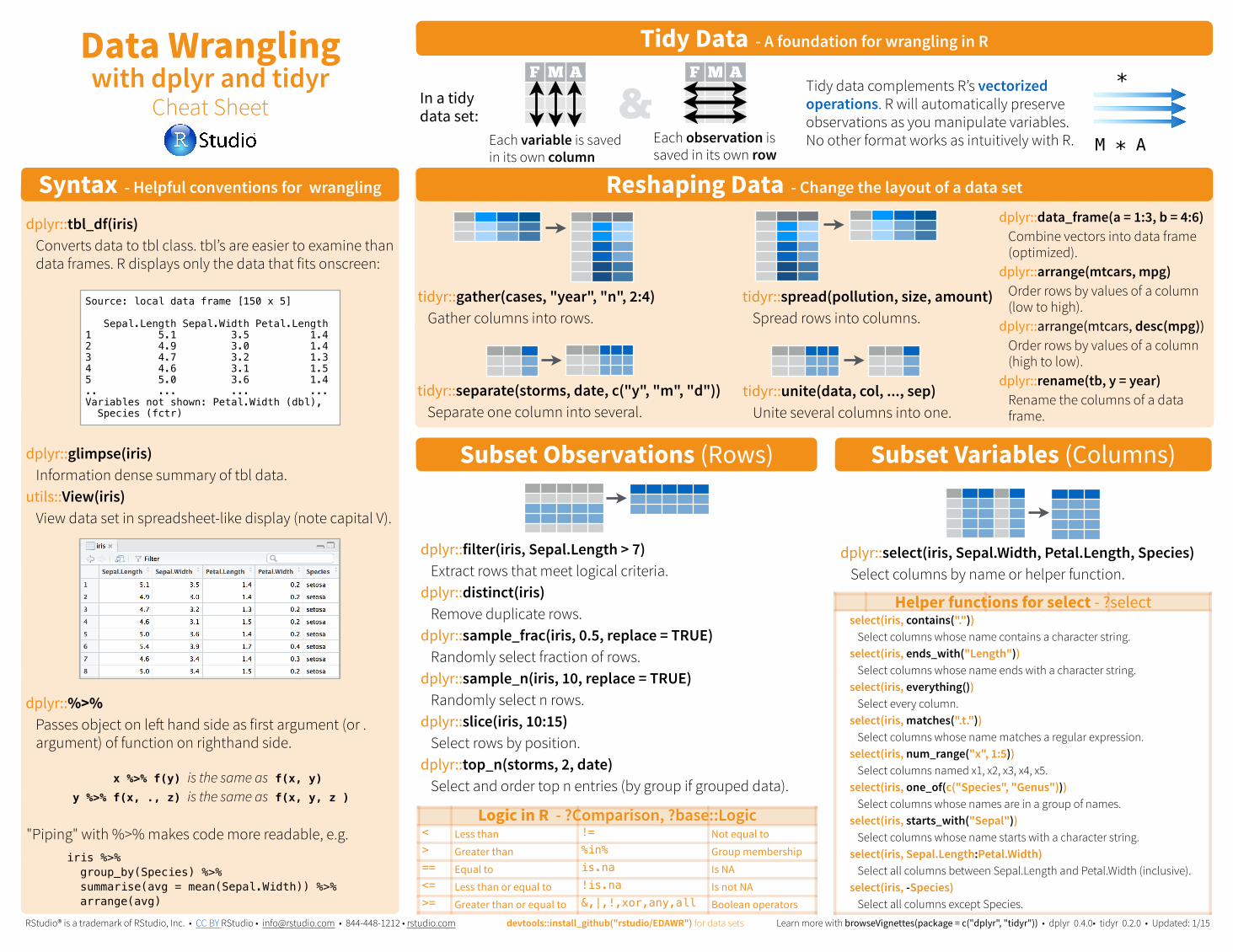
Syntax - Helpful conventions for wrangling
dplyr::tbl_df(iris) Converts data to tbl class. tbl’s are easier to examine than data frames. R displays only the data that fits onscreen:
dplyr::glimpse(iris) Information dense summary of tbl data.
utils::View(iris) View data set in spreadsheet-like display (note capital V).
Source: local data frame [150 x 5]
Sepal.Length Sepal.Width Petal.Length 1 5.1 3.5 1.4 2 4.9 3.0 1.4 3 4.7 3.2 1.3 4 4.6 3.1 1.5 5 5.0 3.6 1.4 .. ... ... ... Variables not shown: Petal.Width (dbl), Species (fctr)
dplyr::%>% Passes object on left hand side as first argument (or . argument) of function on righthand side.
"Piping" with %>% makes code more readable, e.g. iris %>% group_by(Species) %>% summarise(avg = mean(Sepal.Width)) %>% arrange(avg)
x %>% f(y) is the same as f(x, y) y %>% f(x, ., z) is the same as f(x, y, z )
Reshaping Data - Change the layout of a data set
Subset Observations (Rows) Subset Variables (Columns)
F M A
Each variable is saved in its own column
F M A
Each observation is saved in its own row
In a tidy data set: &
Tidy Data - A foundation for wrangling in R
Tidy data complements R’s vectorized operations. R will automatically preserve observations as you manipulate variables. No other format works as intuitively with R.
FAM
M * A
*
tidyr::gather(cases, "year", "n", 2:4) Gather columns into rows.
tidyr::unite(data, col, ..., sep) Unite several columns into one.
dplyr::data_frame(a = 1:3, b = 4:6) Combine vectors into data frame (optimized).
dplyr::arrange(mtcars, mpg) Order rows by values of a column (low to high).
dplyr::arrange(mtcars, desc(mpg)) Order rows by values of a column (high to low).
dplyr::rename(tb, y = year) Rename the columns of a data frame.
tidyr::spread(pollution, size, amount) Spread rows into columns.
tidyr::separate(storms, date, c("y", "m", "d")) Separate one column into several.
wwwwwwA1005A1013A1010A1010
wwp110110100745451009wwp110110100745451009 wwp110110100745451009wwp110110100745451009
wppw11010071007110451009100945wwwww110110110110110 wwwwdplyr::filter(iris, Sepal.Length > 7)
Extract rows that meet logical criteria. dplyr::distinct(iris)
Remove duplicate rows. dplyr::sample_frac(iris, 0.5, replace = TRUE)
Randomly select fraction of rows. dplyr::sample_n(iris, 10, replace = TRUE)
Randomly select n rows. dplyr::slice(iris, 10:15)
Select rows by position. dplyr::top_n(storms, 2, date)
Select and order top n entries (by group if grouped data).
< Less than != Not equal to> Greater than %in% Group membership== Equal to is.na Is NA<= Less than or equal to !is.na Is not NA>= Greater than or equal to &,|,!,xor,any,all Boolean operators
Logic in R - ?Comparison, ?base::Logic
dplyr::select(iris, Sepal.Width, Petal.Length, Species) Select columns by name or helper function.
Helper functions for select - ?selectselect(iris, contains("."))
Select columns whose name contains a character string. select(iris, ends_with("Length"))
Select columns whose name ends with a character string. select(iris, everything())
Select every column. select(iris, matches(".t."))
Select columns whose name matches a regular expression. select(iris, num_range("x", 1:5))
Select columns named x1, x2, x3, x4, x5. select(iris, one_of(c("Species", "Genus")))
Select columns whose names are in a group of names. select(iris, starts_with("Sepal"))
Select columns whose name starts with a character string. select(iris, Sepal.Length:Petal.Width)
Select all columns between Sepal.Length and Petal.Width (inclusive). select(iris, -Species)
Select all columns except Species. Learn more with browseVignettes(package = c("dplyr", "tidyr")) • dplyr 0.4.0• tidyr 0.2.0 • Updated: 1/15
wwwwwwA1005A1013A1010A1010
devtools::install_github("rstudio/EDAWR") for data sets

dplyr::group_by(iris, Species) Group data into rows with the same value of Species.
dplyr::ungroup(iris) Remove grouping information from data frame.
iris %>% group_by(Species) %>% summarise(…) Compute separate summary row for each group.
Combine Data Sets
Group Data
Summarise Data Make New Variables
ir irC
dplyr::summarise(iris, avg = mean(Sepal.Length)) Summarise data into single row of values.
dplyr::summarise_each(iris, funs(mean)) Apply summary function to each column.
dplyr::count(iris, Species, wt = Sepal.Length) Count number of rows with each unique value of variable (with or without weights).
dplyr::mutate(iris, sepal = Sepal.Length + Sepal. Width) Compute and append one or more new columns.
dplyr::mutate_each(iris, funs(min_rank)) Apply window function to each column.
dplyr::transmute(iris, sepal = Sepal.Length + Sepal. Width) Compute one or more new columns. Drop original columns.
Summarise uses summary functions, functions that take a vector of values and return a single value, such as:
Mutate uses window functions, functions that take a vector of values and return another vector of values, such as:
window function
summary function
dplyr::first First value of a vector.
dplyr::last Last value of a vector.
dplyr::nth Nth value of a vector.
dplyr::n # of values in a vector.
dplyr::n_distinct # of distinct values in a vector.
IQR IQR of a vector.
min Minimum value in a vector.
max Maximum value in a vector.
mean Mean value of a vector.
median Median value of a vector.
var Variance of a vector.
sd Standard deviation of a vector.
dplyr::lead Copy with values shifted by 1.
dplyr::lag Copy with values lagged by 1.
dplyr::dense_rank Ranks with no gaps.
dplyr::min_rank Ranks. Ties get min rank.
dplyr::percent_rank Ranks rescaled to [0, 1].
dplyr::row_number Ranks. Ties got to first value.
dplyr::ntile Bin vector into n buckets.
dplyr::between Are values between a and b?
dplyr::cume_dist Cumulative distribution.
dplyr::cumall Cumulative all
dplyr::cumany Cumulative any
dplyr::cummean Cumulative mean
cumsum Cumulative sum
cummax Cumulative max
cummin Cumulative min
cumprod Cumulative prod
pmax Element-wise max
pmin Element-wise min
iris %>% group_by(Species) %>% mutate(…) Compute new variables by group.
x1 x2A 1B 2C 3
x1 x3A TB FD T+ =
x1 x2 x3A 1 TB 2 FC 3 NA
x1 x3 x2A T 1B F 2D T NA
x1 x2 x3A 1 TB 2 F
x1 x2 x3A 1 TB 2 FC 3 NAD NA T
x1 x2A 1B 2C 3
x1 x2B 2C 3D 4+ =
x1 x2B 2C 3
x1 x2A 1B 2C 3D 4
x1 x2A 1
x1 x2A 1B 2C 3B 2C 3D 4
x1 x2 x1 x2A 1 B 2B 2 C 3C 3 D 4
Mutating Joins
Filtering Joins
Binding
Set Operations
dplyr::left_join(a, b, by = "x1") Join matching rows from b to a.
a b
dplyr::right_join(a, b, by = "x1") Join matching rows from a to b.
dplyr::inner_join(a, b, by = "x1") Join data. Retain only rows in both sets.
dplyr::full_join(a, b, by = "x1") Join data. Retain all values, all rows.
x1 x2A 1B 2
x1 x2C 3
y z
dplyr::semi_join(a, b, by = "x1") All rows in a that have a match in b.
dplyr::anti_join(a, b, by = "x1") All rows in a that do not have a match in b.
dplyr::intersect(y, z) Rows that appear in both y and z.
dplyr::union(y, z) Rows that appear in either or both y and z.
dplyr::setdiff(y, z) Rows that appear in y but not z.
dplyr::bind_rows(y, z) Append z to y as new rows.
dplyr::bind_cols(y, z) Append z to y as new columns. Caution: matches rows by position.
RStudio® is a trademark of RStudio, Inc. • CC BY RStudio • [email protected] • 844-448-1212 • rstudio.com Learn more with browseVignettes(package = c("dplyr", "tidyr")) • dplyr 0.4.0• tidyr 0.2.0 • Updated: 1/15devtools::install_github("rstudio/EDAWR") for data sets

Geoms - Use a geom to represent data points, use the geom’s aesthetic properties to represent variables. Each function returns a layer.
Graphical Primitives a <- ggplot(seals, aes(x = long, y = lat))
b <- ggplot(economics, aes(date, unemploy))
a + geom_blank() (Useful for expanding limits)
a + geom_curve(aes(yend = lat + delta_lat, xend = long + delta_long, curvature = z)) x, xend, y, yend, alpha, angle, color, curvature, linetype, size
b + geom_path(lineend="butt", linejoin="round’, linemitre=1) x, y, alpha, color, group, linetype, size
b + geom_polygon(aes(group = group)) x, y, alpha, color, fill, group, linetype, size
a + geom_rect(aes(xmin = long, ymin = lat, xmax= long + delta_long, ymax = lat + delta_lat)) xmax, xmin, ymax, ymin, alpha, color, fill, linetype, size
b + geom_ribbon(aes(ymin=unemploy - 900, ymax=unemploy + 900)) x, ymax, ymin, alpha, color, fill, group, linetype, size
a + geom_segment(aes(yend=lat + delta_lat, xend = long + delta_long)) x, xend, y, yend, alpha, color, linetype, size
a + geom_spoke(aes(yend = lat + delta_lat, xend = long + delta_long)) x, y, angle, radius, alpha, color, linetype, size
One Variable
c + geom_area(stat = "bin") x, y, alpha, color, fill, linetype, size a + geom_area(aes(y = ..density..), stat = "bin")
c + geom_density(kernel = "gaussian") x, y, alpha, color, fill, group, linetype, size, weight
c + geom_dotplot() x, y, alpha, color, fill
c + geom_freqpoly() x, y, alpha, color, group, linetype, size a + geom_freqpoly(aes(y = ..density..))
c + geom_histogram(binwidth = 5) x, y, alpha, color, fill, linetype, size, weight a + geom_histogram(aes(y = ..density..))
Discreted <- ggplot(mpg, aes(fl))
d + geom_bar() x, alpha, color, fill, linetype, size, weight
Continuousc <- ggplot(mpg, aes(hwy))
Three Variables
l + geom_contour(aes(z = z)) x, y, z, alpha, colour, group, linetype, size, weight
seals$z <- with(seals, sqrt(delta_long^2 + delta_lat^2)) l <- ggplot(seals, aes(long, lat))
l + geom_raster(aes(fill = z), hjust=0.5, vjust=0.5, interpolate=FALSE) x, y, alpha, fill
l + geom_tile(aes(fill = z)) x, y, alpha, color, fill, linetype, size, width
Two Variables
Discrete X, Discrete Yg <- ggplot(diamonds, aes(cut, color))
g + geom_count() x, y, alpha, color, fill, shape, size, stroke
Discrete X, Continuous Yf <- ggplot(mpg, aes(class, hwy))
f + geom_bar(stat = "identity") x, y, alpha, color, fill, linetype, size, weight
f + geom_boxplot() x, y, lower, middle, upper, ymax, ymin, alpha, color, fill, group, linetype, shape, size, weight
f + geom_dotplot(binaxis = "y", stackdir = "center") x, y, alpha, color, fill, group
f + geom_violin(scale = "area") x, y, alpha, color, fill, group, linetype, size, weight
Continuous X, Continuous Ye <- ggplot(mpg, aes(cty, hwy))
e + geom_label(aes(label = cty), nudge_x = 1, nudge_y = 1, check_overlap = TRUE) x, y, label, alpha, angle, color, family, fontface, hjust, lineheight, size, vjust
e + geom_jitter(height = 2, width = 2) x, y, alpha, color, fill, shape, size
e + geom_point() x, y, alpha, color, fill, shape, size, stroke
e + geom_quantile() x, y, alpha, color, group, linetype, size, weight
e + geom_rug(sides = "bl") x, y, alpha, color, linetype, size
e + geom_smooth(method = lm) x, y, alpha, color, fill, group, linetype, size, weight
e + geom_text(aes(label = cty), nudge_x = 1, nudge_y = 1, check_overlap = TRUE) x, y, label, alpha, angle, color, family, fontface, hjust, lineheight, size, vjust
ABC
AB
C
Continuous Functioni <- ggplot(economics, aes(date, unemploy))
i + geom_area() x, y, alpha, color, fill, linetype, size
i + geom_line() x, y, alpha, color, group, linetype, size
i + geom_step(direction = "hv") x, y, alpha, color, group, linetype, size
Continuous Bivariate Distributionh <- ggplot(diamonds, aes(carat, price))
j + geom_crossbar(fatten = 2) x, y, ymax, ymin, alpha, color, fill, group, linetype, size
j + geom_errorbar() x, ymax, ymin, alpha, color, group, linetype, size, width (also geom_errorbarh())
j + geom_linerange() x, ymin, ymax, alpha, color, group, linetype, size
j + geom_pointrange() x, y, ymin, ymax, alpha, color, fill, group, linetype, shape, size
Visualizing errordf <- data.frame(grp = c("A", "B"), fit = 4:5, se = 1:2)
j <- ggplot(df, aes(grp, fit, ymin = fit-se, ymax = fit+se))
data <- data.frame(murder = USArrests$Murder, state = tolower(rownames(USArrests)))
map <- map_data("state") k <- ggplot(data, aes(fill = murder))
k + geom_map(aes(map_id = state), map = map) + expand_limits(x = map$long, y = map$lat) map_id, alpha, color, fill, linetype, size
Maps
h + geom_bin2d(binwidth = c(0.25, 500)) x, y, alpha, color, fill, linetype, size, weight
h + geom_density2d() x, y, alpha, colour, group, linetype, size
h + geom_hex() x, y, alpha, colour, fill, size
Basics
Build a graph with ggplot() or qplot()
ggplot2 is based on the grammar of graphics, the idea that you can build every graph from the same few components: a data set, a set of geoms—visual marks that represent data points, and a coordinate system.
To display data values, map variables in the data set to aesthetic properties of the geom like size, color, and x and y locations.
Graphical Primitives
Data Visualization with ggplot2
Cheat Sheet
RStudio® is a trademark of RStudio, Inc. • CC BY RStudio • [email protected] • 844-448-1212 • rstudio.com Learn more at docs.ggplot2.org • ggplot2 0.9.3.1 • Updated: 3/15
Geoms - Use a geom to represent data points, use the geom’s aesthetic properties to represent variables
Basics
One Variable
a + geom_area(stat = "bin") x, y, alpha, color, fill, linetype, size b + geom_area(aes(y = ..density..), stat = "bin")
a + geom_density(kernal = "gaussian") x, y, alpha, color, fill, linetype, size, weight b + geom_density(aes(y = ..county..))
a+ geom_dotplot() x, y, alpha, color, fill
a + geom_freqpoly() x, y, alpha, color, linetype, size b + geom_freqpoly(aes(y = ..density..))
a + geom_histogram(binwidth = 5) x, y, alpha, color, fill, linetype, size, weight b + geom_histogram(aes(y = ..density..))
Discretea <- ggplot(mpg, aes(fl))
b + geom_bar() x, alpha, color, fill, linetype, size, weight
Continuousa <- ggplot(mpg, aes(hwy))
Two Variables
Discrete X, Discrete Yh <- ggplot(diamonds, aes(cut, color))
h + geom_jitter() x, y, alpha, color, fill, shape, size
Discrete X, Continuous Yg <- ggplot(mpg, aes(class, hwy))
g + geom_bar(stat = "identity") x, y, alpha, color, fill, linetype, size, weight
g + geom_boxplot() lower, middle, upper, x, ymax, ymin, alpha, color, fill, linetype, shape, size, weight
g + geom_dotplot(binaxis = "y", stackdir = "center") x, y, alpha, color, fill
g + geom_violin(scale = "area") x, y, alpha, color, fill, linetype, size, weight
Continuous X, Continuous Yf <- ggplot(mpg, aes(cty, hwy))
f + geom_blank()
f + geom_jitter() x, y, alpha, color, fill, shape, size
f + geom_point() x, y, alpha, color, fill, shape, size
f + geom_quantile() x, y, alpha, color, linetype, size, weight
f + geom_rug(sides = "bl") alpha, color, linetype, size
f + geom_smooth(model = lm) x, y, alpha, color, fill, linetype, size, weight
f + geom_text(aes(label = cty)) x, y, label, alpha, angle, color, family, fontface, hjust, lineheight, size, vjust
Three Variables
i + geom_contour(aes(z = z)) x, y, z, alpha, colour, linetype, size, weight
seals$z <- with(seals, sqrt(delta_long^2 + delta_lat^2)) i <- ggplot(seals, aes(long, lat))
g <- ggplot(economics, aes(date, unemploy))Continuous Function
g + geom_area() x, y, alpha, color, fill, linetype, size
g + geom_line() x, y, alpha, color, linetype, size
g + geom_step(direction = "hv") x, y, alpha, color, linetype, size
Continuous Bivariate Distributionh <- ggplot(movies, aes(year, rating))h + geom_bin2d(binwidth = c(5, 0.5))
xmax, xmin, ymax, ymin, alpha, color, fill, linetype, size, weight
h + geom_density2d() x, y, alpha, colour, linetype, size
h + geom_hex() x, y, alpha, colour, fill size
d + geom_segment(aes( xend = long + delta_long, yend = lat + delta_lat)) x, xend, y, yend, alpha, color, linetype, size
d + geom_rect(aes(xmin = long, ymin = lat, xmax= long + delta_long, ymax = lat + delta_lat)) xmax, xmin, ymax, ymin, alpha, color, fill, linetype, size
c + geom_polygon(aes(group = group)) x, y, alpha, color, fill, linetype, size
d<- ggplot(seals, aes(x = long, y = lat))
i + geom_raster(aes(fill = z), hjust=0.5, vjust=0.5, interpolate=FALSE) x, y, alpha, fill
i + geom_tile(aes(fill = z)) x, y, alpha, color, fill, linetype, size
e + geom_crossbar(fatten = 2) x, y, ymax, ymin, alpha, color, fill, linetype, size
e + geom_errorbar() x, ymax, ymin, alpha, color, linetype, size, width (also geom_errorbarh())
e + geom_linerange() x, ymin, ymax, alpha, color, linetype, size
e + geom_pointrange() x, y, ymin, ymax, alpha, color, fill, linetype, shape, size
Visualizing errordf <- data.frame(grp = c("A", "B"), fit = 4:5, se = 1:2)
e <- ggplot(df, aes(grp, fit, ymin = fit-se, ymax = fit+se))
g + geom_path(lineend="butt", linejoin="round’, linemitre=1) x, y, alpha, color, linetype, size
g + geom_ribbon(aes(ymin=unemploy - 900, ymax=unemploy + 900)) x, ymax, ymin, alpha, color, fill, linetype, size
g <- ggplot(economics, aes(date, unemploy))
c <- ggplot(map, aes(long, lat))
data <- data.frame(murder = USArrests$Murder, state = tolower(rownames(USArrests)))
map <- map_data("state") e <- ggplot(data, aes(fill = murder))
e + geom_map(aes(map_id = state), map = map) + expand_limits(x = map$long, y = map$lat) map_id, alpha, color, fill, linetype, size
Maps
F M A
=1
2
3
00 1 2 3 4
4
1
2
3
00 1 2 3 4
4
+
data geom coordinate system
plot
+
F M A
=1
2
3
00 1 2 3 4
4
1
2
3
00 1 2 3 4
4
data geom coordinate system
plotx = F y = A color = F size = A
1
2
3
00 1 2 3 4
4
plot
+
F M A
=1
2
3
00 1 2 3 4
4
data geom coordinate systemx = F
y = A
x = F y = A
ggsave("plot.png", width = 5, height = 5) Saves last plot as 5’ x 5’ file named "plot.png" in working directory. Matches file type to file extension.
qplot(x = cty, y = hwy, color = cyl, data = mpg, geom = "point") Creates a complete plot with given data, geom, and mappings. Supplies many useful defaults.
aesthetic mappings data geom
ggplot(data = mpg, aes(x = cty, y = hwy)) Begins a plot that you finish by adding layers to. No defaults, but provides more control than qplot().
ggplot(mpg, aes(hwy, cty)) + geom_point(aes(color = cyl)) + geom_smooth(method ="lm") + coord_cartesian() + scale_color_gradient() + theme_bw()
dataadd layers,
elements with +
layer = geom + default stat + layer specific
mappings
additional elements
Add a new layer to a plot with a geom_*() or stat_*() function. Each provides a geom, a set of aesthetic mappings, and a default stat
and position adjustment.
last_plot() Returns the last plot
Data Visualization with ggplot2
Cheat Sheet
RStudio® is a trademark of RStudio, Inc. • CC BY RStudio • [email protected] • 844-448-1212 • rstudio.com Learn more at docs.ggplot2.org • ggplot2 2.0.0 • Updated: 12/15

RStudio® is a trademark of RStudio, Inc. • CC BY RStudio • [email protected] • 844-448-1212 • rstudio.com
Stats - An alternative way to build a layer
Each stat creates additional variables to map aesthetics to. These variables use a common ..name.. syntax.
stat and geom functions both combine a stat with a geom to make a layer, i.e. stat_count(geom="bar") does the same as geom_bar(stat="count")
+x ..count..
=1
2
3
00 1 2 3 4
4
1
2
3
00 1 2 3 4
4
data geom coordinate system
plotx = x y = ..count..
fl cty cyl
stat
ggplot() + stat_function(aes(x = -3:3), fun = dnorm, n = 101, args = list(sd=0.5)) x | ..x.., ..y..
e + stat_identity(na.rm = TRUE) ggplot() + stat_qq(aes(sample=1:100), distribution = qt,
dparams = list(df=5)) sample, x, y | ..sample.., ..theoretical..
e + stat_sum() x, y, size | ..n.., ..prop..
e + stat_summary(fun.data = "mean_cl_boot") h + stat_summary_bin(fun.y = "mean", geom = "bar") e + stat_unique()
i + stat_density2d(aes(fill = ..level..), geom = "polygon", n = 100)
stat function layer mappings
variable created by
transformationgeom for layer parameters for stat
c + stat_bin(binwidth = 1, origin = 10) x, y | ..count.., ..ncount.., ..density.., ..ndensity..
c + stat_count(width = 1) x, y, | ..count.., ..prop..
c + stat_density(adjust = 1, kernel = "gaussian") x, y, | ..count.., ..density.., ..scaled..
e + stat_bin_2d(bins = 30, drop = TRUE) x, y, fill | ..count.., ..density..
e + stat_bin_hex(bins = 30) x, y, fill | ..count.., ..density..
e + stat_density_2d(contour = TRUE, n = 100) x, y, color, size | ..level..
e + stat_ellipse(level = 0.95, segments = 51, type = "t")
l + stat_contour(aes(z = z)) x, y, z, order | ..level..
l + stat_summary_hex(aes(z = z), bins = 30, fun = mean) x, y, z, fill | ..value..
l + stat_summary_2d(aes(z = z), bins = 30, fun = mean) x, y, z, fill | ..value..
f + stat_boxplot(coef = 1.5) x, y | ..lower.., ..middle.., ..upper.., ..width.. , ..ymin.., ..ymax..
f + stat_ydensity(adjust = 1, kernel = "gaussian", scale = "area") x, y | ..density.., ..scaled.., ..count.., ..n.., ..violinwidth.., ..width..
e + stat_ecdf(n = 40) x, y | ..x.., ..y..
e + stat_quantile(quantiles = c(0.25, 0.5, 0.75), formula = y ~ log(x), method = "rq") x, y | ..quantile..
e + stat_smooth(method = "auto", formula = y ~ x, se = TRUE, n = 80, fullrange = FALSE, level = 0.95) x, y | ..se.., ..x.., ..y.., ..ymin.., ..ymax..
1D distributions
2D distributions
3 Variables
Comparisons
Functions
General Purpose
Some plots visualize a transformation of the original data set. Use a stat to choose a common transformation to visualize, e.g. a + geom_bar(stat = "count")
ScalesScales control how a plot maps data values to the visual values of an aesthetic. To change the mapping, add a custom scale.
n <- b + geom_bar(aes(fill = fl)) n
n + scale_fill_manual( values = c("skyblue", "royalblue", "blue", "navy"), limits = c("d", "e", "p", "r"), breaks =c("d", "e", "p", "r"), name = "fuel", labels = c("D", "E", "P", "R"))
scale_ aesthetic to adjust
prepackaged scale to use
scale specific arguments
range of values to include in mapping
title to use in legend/axis
labels to use in legend/axis
breaks to use in legend/axis
General Purpose scalesUse with any aesthetic:
alpha, color, fill, linetype, shape, size
scale_*_continuous() - map cont’ values to visual values scale_*_discrete() - map discrete values to visual values scale_*_identity() - use data values as visual values scale_*_manual(values = c()) - map discrete values to
manually chosen visual values
X and Y location scales
Color and fill scales
Shape scales
Size scales
Use with x or y aesthetics (x shown here) scale_x_date(date_labels = "%m/%d"),
date_breaks = "2 weeks") - treat x values as dates. See ?strptime for label formats.
scale_x_datetime() - treat x values as date times. Use same arguments as scale_x_date().
scale_x_log10() - Plot x on log10 scale scale_x_reverse() - Reverse direction of x axis scale_x_sqrt() - Plot x on square root scale
Discrete Continuous
n <- d + geom_bar( aes(fill = fl))
o <- c + geom_dotplot( aes(fill = ..x..))
n + scale_fill_brewer( palette = "Blues") For palette choices: library(RColorBrewer) display.brewer.all()
n + scale_fill_grey( start = 0.2, end = 0.8, na.value = "red")
o + scale_fill_gradient( low = "red", high = "yellow")
o + scale_fill_gradient2( low = "red", high = "blue", mid = "white", midpoint = 25)
o + scale_fill_gradientn( colours = terrain.colors(6))
Also: rainbow(), heat.colors(), topo.colors(), cm.colors(), RColorBrewer::brewer.pal()
p <- e + geom_point(aes( shape = fl, size = cyl))
p + scale_shape( solid = FALSE)
p + scale_shape_manual( values = c(3:7)) Shape values shown in chart on right
Manual Shape values
0
1
2
3
4
5
6
7
8
9
10
11
12
13
14
15
16
17
18
19
20
21
22
23
24
25
**.
ooOO
00++--||%%##
Manual shape values
p + scale_size_area( max_scale = 6) Maps to area of circle (not radius)
p + scale_radius( range=c(1,6))
p + scale_size()
Coordinate Systems
r + coord_cartesian(xlim = c(0, 5)) xlim, ylim The default cartesian coordinate system
r + coord_fixed(ratio = 1/2) ratio, xlim, ylim Cartesian coordinates with fixed aspect ratio between x and y units
r + coord_flip() xlim, ylim Flipped Cartesian coordinates
r + coord_polar(theta = "x", direction=1 ) theta, start, direction Polar coordinates
r + coord_trans(ytrans = "sqrt") xtrans, ytrans, limx, limy Transformed cartesian coordinates. Set xtrans and ytrans to the name of a window function.
r <- d + geom_bar()
60
long
lat
π + coord_map(projection = "ortho", orientation=c(41, -74, 0))
projection, orientation, xlim, ylim Map projections from the mapproj package (mercator (default), azequalarea, lagrange, etc.)
Learn more at docs.ggplot2.org • ggplot2 2.0.0 • Updated: 12/15
Position Adjustments
s + geom_bar(position = "dodge") Arrange elements side by side
s + geom_bar(position = "fill") Stack elements on top of one another, normalize height
e + geom_point(position = "jitter") Add random noise to X and Y position of each element to avoid overplotting
e + geom_label(position = "nudge") Nudge labels away from points
s + geom_bar(position = "stack") Stack elements on top of one another
s <- ggplot(mpg, aes(fl, fill = drv))
Position adjustments determine how to arrange geoms that would otherwise occupy the same space.
Each position adjustment can be recast as a function with manual width and height arguments
s + geom_bar(position = position_dodge(width = 1))
AB
Themes r + theme_classic()
r + theme_light() r + theme_linedraw() r + theme_minimal()
Minimal themes r + theme_void()
Empty theme
0
50
100
150
c d e p rfl
count
0
50
100
150
c d e p rfl
count
0
50
100
150
c d e p rfl
count
0
50
100
150
c d e p rfl
countr + theme_bw()
White background with grid lines
r + theme_gray() Grey background (default theme)
r + theme_dark() dark for contrast 0
50
100
150
c d e p rfl
count
Zooming
t + coord_cartesian( xlim = c(0, 100), ylim = c(10, 20))
With clipping (removes unseen data points)t + xlim(0, 100) + ylim(10, 20) t + scale_x_continuous(limits = c(0, 100)) +
scale_y_continuous(limits = c(0, 100))
Without clipping (preferred)
Legends n + theme(legend.position = "bottom")
Place legend at "bottom", "top", "left", or "right" n + guides(fill = "none")
Set legend type for each aesthetic: colorbar, legend, or none (no legend)
n + scale_fill_discrete(name = "Title", labels = c("A", "B", "C", "D", "E")) Set legend title and labels with a scale function.
Labels t + ggtitle("New Plot Title")
Add a main title above the plot t + xlab("New X label")
Change the label on the X axis t + ylab("New Y label")
Change the label on the Y axis t + labs(title =" New title", x = "New x", y = "New y")
All of the above
Use scale functions to update legend
labels
Faceting
t <- ggplot(mpg, aes(cty, hwy)) + geom_point()
Facets divide a plot into subplots based on the values of one or more discrete variables.
t + facet_grid(. ~ fl) facet into columns based on fl
t + facet_grid(year ~ .) facet into rows based on year
t + facet_grid(year ~ fl) facet into both rows and columns
t + facet_wrap(~ fl) wrap facets into a rectangular layout
Set scales to let axis limits vary across facets
t + facet_grid(drv ~ fl, scales = "free") x and y axis limits adjust to individual facets • "free_x" - x axis limits adjust • "free_y" - y axis limits adjust
Set labeller to adjust facet labels
t + facet_grid(. ~ fl, labeller = label_both)
t + facet_grid(fl ~ ., labeller = label_bquote(alpha ^ .(fl)))
t + facet_grid(. ~ fl, labeller = label_parsed)
fl: c fl: d fl: e fl: p fl: r
c d e p r
↵c ↵d ↵e ↵p ↵r
render()
RStudio Pro FeaturesWorkflow
Debug ModeEmbed code with knitr syntax
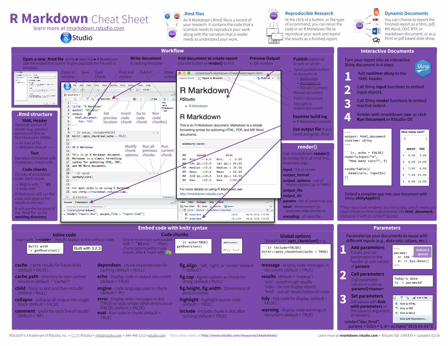
learn more at rmarkdown.rstudio.com
Rmd Reproducible Research At the click of a button, or the type of a command, you can rerun the code in an R Markdown file to reproduce your work and export the results as a finished report.
Use rmarkdown::render() to render/knit at cmd line. Important args:
input - file to render output_format output_options - List of
render options (as in YAML) output_file output_dir params - list of params to use envir - environment to
evaluate code chunks in encoding - of input file
R Markdown Cheat Sheet
RStudio® is a trademark of RStudio, Inc. • CC BY RStudio • [email protected] • 844-448-1212 • rstudio.com Learn more at rmarkdown.rstudio.com • RStudio IDE 0.99.879 • Updated: 02/16More cheat sheets at http://www.rstudio.com/resources/cheatsheets/
Debug ModeParameters
.Rmd files An R Markdown (.Rmd) file is a record of your research. It contains the code that a scientist needs to reproduce your work along with the narration that a reader needs to understand your work.
Dynamic Documents You can choose to export the finished report as a html, pdf, MS Word, ODT, RTF, or markdown document; or as a html or pdf based slide show.
Rmd
.Rmd structure
Modify chunk options
Run all previous chunks
Run current chunk
Insert code chunk
Go to code chunk
Run code chunk(s)
Set preview location
Open in window
Save Find and replace
Open a new .Rmd file at File ▶ New File ▶ R Markdown. Use the wizard that opens to pre-populate the file with a template
1 Write document by editing template2
Spell Check
Publish Show outline
Knit document to create report Use knit button or render() to knit3
Examine build log in R Markdown console6
Preview Output in IDE window4
Use output file that is saved alongside .Rmd7
Publish (optional) to web or server5
Reload documentFind in documentFile path to output document
Synch publish button to accounts at
• rpubs.com, • shinyapps.io • RStudio Connect
Debug ModeInteractive Documents
Optional section of render (e.g. pandoc) options written as key:value pairs (YAML).
• At start of file • Between lines of - - -
YAML Header
Narration formatted with markdown, mixed with:
Text
Chunks of embedded code. Each chunk:
• Begins with ```{r} • ends with ```
R Markdown will run the code and append the results to the doc. It will use the location of the .Rmd file as the working directory
Code chunks
Turn your report into an interactive Shiny document in 4 steps
* Your report will rendered as a Shiny app, which means you must choose an html output format, like html_document, and serve it with an active R Session.
1 Add runtime: shiny to the YAML header.
2 Call Shiny input functions to embed input objects.
4 Render with rmarkdown::run or click Run Document in RStudio IDE
3 Call Shiny render functions to embed reactive output.
--- output: html_document runtime: shiny ---
```{r, echo = FALSE} numericInput("n", "How many cars?", 5)
renderTable({ head(cars, input$n) }) ```
Embed a complete app into your document with shiny::shinyAppDir()
Inline codeInsert with `r <code>`. Results appear as text without code.
Built with `r getRversion()`
Global optionsSet with knitr::opts_chunk$set(), e.g.
```{r include=FALSE} knitr::opts_chunk$set(echo = TRUE) ```
```{r echo=TRUE} getRversion() ```
Code chunksOne or more lines surrounded with ```{r} and ```. Place chunk options within curly braces, after r. Insert with
cache - cache results for future knits (default = FALSE)
cache.path - directory to save cached results in (default = "cache/")
child - file(s) to knit and then include (default = NULL)
collapse - collapse all output into single block (default = FALSE)
comment - prefix for each line of results (default = '##')
dependson - chunk dependencies for caching (default = NULL)
echo - Display code in output document (default = TRUE)
engine - code language used in chunk (default = 'R')
error - Display error messages in doc (TRUE) or stop render when errors occur (FALSE) (default = FALSE)
eval - Run code in chunk (default = TRUE)
message - display code messages in document (default = TRUE)
results (default = 'markup') 'asis' - passthrough results 'hide' - do not display results 'hold' - put all results below all code
tidy - tidy code for display (default = FALSE)
warning - display code warnings in document (default = TRUE)
fig.align - 'left', 'right', or 'center' (default = 'default')
fig.cap - figure caption as character string (default = NULL)
fig.height, fig.width - Dimensions of plots in inches
highlight - highlight source code (default = TRUE)
include - Include chunk in doc after running (default = TRUE)
Important chunk options
Parameterize your documents to reuse with different inputs (e.g., data sets, values, etc.)
Add parameters1 Create and set parameters in the header as sub-values of params
--- params: n: 100 d: !r Sys.Date() ---
Call parameters2 Call parameter values in code as params$<name>
Today’s date is `r params$d`
Set parameters3 Set values wth Knit with parameters or the params argument of render():
render("doc.Rmd", params = list(n = 1, d = as.Date("2015-01-01"))
Indent 2 spaces
Options not listed above: R.options, aniopts, autodep, background, cache.comments, cache.lazy, cache.rebuild, cache.vars, dev, dev.args, dpi, engine.opts, engine.path, fig.asp, fig.env, fig.ext, fig.keep, fig.lp, fig.path, fig.pos, fig.process, fig.retina, fig.scap, fig.show, fig.showtext, fig.subcap, interval, out.extra, out.height, out.width, prompt, purl, ref.label, render, size, split, tidy.opts

RStudio® is a trademark of RStudio, Inc. • CC BY RStudio • [email protected] • 844-448-1212 • rstudio.com More cheat sheets at http://www.rstudio.com/resources/cheatsheets/
Debug ModePandoc’s Markdown Debug ModeSet render options with YAML
Plain text End a line with two spaces to start a new paragraph. *italics* and **bold** `verbatim code` sub/superscript^2^~2~ ~~strikethrough~~ escaped: \* \_ \\ endash: --, emdash: --- equation: $A = \pi*r^{2}$ equation block:
$$E = mc^{2}$$ > block quote # Header1 {#anchor}
## Header 2 {#css_id} ### Header 3 {.css_class}
#### Header 4 ##### Header 5 ###### Header 6
<!--Text comment--> \textbf{Tex ignored in HTML} <em>HTML ignored in pdfs</em>
<http://www.rstudio.com> [link](www.rstudio.com) Jump to [Header 1](#anchor) image:
 * unordered list + sub-item 1 + sub-item 2 - sub-sub-item 1 * item 2 Continued (indent 4 spaces) 1. ordered list 2. item 2 i) sub-item 1 A. sub-sub-item 1
(@) A list whose numbering continues after
(@) an interruption Term 1 : Definition 1 | Right | Left | Default | Center | |------:|:-----|---------|:------:| | 12 | 12 | 12 | 12 | | 123 | 123 | 123 | 123 | | 1 | 1 | 1 | 1 |
- slide bullet 1 - slide bullet 2
(>- to have bullets appear on click)
horizontal rule/slide break: ***
A footnote [^1] [^1]: Here is the footnote.
Debug ModeCitations and Bibliographies
Set bibliography file and CSL 1.0 Style file (optional) in the YAML header1
Use citation keys in text2Render. Bibliography will be added to end of document3
Create citations with .bib, .bibtex, .copac, .enl, .json, .medline, .mods, .ris, .wos, and .xml files
Smith cited [@smith04]. Smith cited without author [-@smith04]. @smith04 cited in line.
--- bibliography: refs.bib csl: style.csl ---
Debug ModeCreate a Reusable template
1 Create a new package with a inst/rmarkdown/templates directory
2 In the directory, Place a folder that contains: • template.yaml (see below) • skeleton.Rmd (contents of the template) • any supporting files
4 Access template in wizard at File ▶ New File ▶ R Markdown
3 Install the package
--- name: My Template ---
template.yaml
Write with syntax on the left to create effect on right (after render)
Debug ModeTable suggestionsSeveral functions format R data into tables
data <- faithful[1:4, ]
```{r results = "asis"} print(xtable::xtable(data, caption = "Table with xtable"), type = "html", html.table.attributes = "border=0")) ```
```{r results = "asis"} stargazer::stargazer(data, type = "html", title = "Table with stargazer") ```
```{r results = 'asis'} knitr::kable(data, caption = "Table with kable") ```
sub-option description
citation_package The LaTeX package to process citations, natbib, biblatex or none X X Xcode_folding Let readers to toggle the display of R code, "none", "hide", or "show" Xcolortheme Beamer color theme to use Xcss CSS file to use to style document X X Xdev Graphics device to use for figure output (e.g. "png") X X X X X X Xduration Add a countdown timer (in minutes) to footer of slides Xfig_caption Should figures be rendered with captions? X X X X X X Xfig_height, fig_width Default figure height and width (in inches) for document X X X X X X X X X Xhighlight Syntax highlighting: "tango", "pygments", "kate","zenburn", "textmate" X X X X Xincludes File of content to place in document (in_header, before_body, after_body) X X X X X X X Xincremental Should bullets appear one at a time (on presenter mouse clicks)? X X Xkeep_md Save a copy of .md file that contains knitr output X X X X X Xkeep_tex Save a copy of .tex file that contains knitr output X Xlatex_engine Engine to render latex, "pdflatex", "xelatex", or "lualatex" X Xlib_dir Directory of dependency files to use (Bootstrap, MathJax, etc.) X X Xmathjax Set to local or a URL to use a local/URL version of MathJax to render X X Xmd_extensions Markdown extensions to add to default definition or R Markdown X X X X X X X X X Xnumber_sections Add section numbering to headers X Xpandoc_args Additional arguments to pass to Pandoc X X X X X X X X X Xpreserve_yaml Preserve YAML front matter in final document? Xreference_docx docx file whose styles should be copied when producing docx output Xself_contained Embed dependencies into the doc X X Xslide_level The lowest heading level that defines individual slides Xsmaller Use the smaller font size in the presentation? Xsmart Convert straight quotes to curly, dashes to em-dashes, … to ellipses, etc. X X Xtemplate Pandoc template to use when rendering file X X X X Xtheme Bootswatch or Beamer theme to use for page X Xtoc Add a table of contents at start of document X X X X X X Xtoc_depth The lowest level of headings to add to table of contents X X X X X Xtoc_float Float the table of contents to the left of the main content X
htm
lpd
fw
ord
odt
rtf
md
iosl
ides
slid
ybe
amer
Options not listed: extra_dependencies, fig_crop, fig_retina, font_adjustment, font_theme, footer, logo, html_preview, reference_odt, transition, variant, widescreen
When you render, R Markdown 1. runs the R code, embeds results and text into .md file with knitr 2. then converts the .md file into the finished format with pandoc
Set a document’s default output format in the YAML header:
--- output: html_document --- # Body
output value createshtml_document htmlpdf_document pdf (requires Tex )word_document Microsoft Word (.docx)odt_document OpenDocument Textrtf_document Rich Text Formatmd_document Markdowngithub_document Github compatible markdownioslides_presentation ioslides HTML slidesslidy_presentation slidy HTML slidesbeamer_presentation Beamer pdf slides (requires Tex)
Customize output with sub-options (listed at right):
--- output: html_document: code_folding: hide toc_float: TRUE --- # Body
Indent 2 spaces
Indent 4 spaces
# Tabset {.tabset .tabset-fade .tabset-pills} ## Tab 1 text 1 ## Tab 2 text 2 ### End tabset
Use .tabset css class to place sub-headers into tabs
html tabsets
gitu
hb
Learn more in the stargazer,
xtable, and knitr packages.
Learn more at rmarkdown.rstudio.com • RStudio IDE 0.99.879 • Updated: 02/16
Cheat Sheet
Updated: 09/16
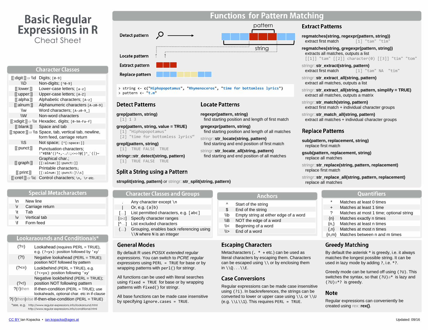
* Matches at least 0 times
+ Matches at least 1 time
? Matches at most 1 time; optional string
{n} Matches exactly n times
{n,} Matches at least n times
{,n} Matches at most n times
{n,m} Matches between n and m times
> string <- c("Hiphopopotamus", "Rhymenoceros", "time for bottomless lyrics") > pattern <- "t.m"
grep(pattern, string) [1] 1 3
grep(pattern, string, value = TRUE) [1] "Hiphopopotamus" [2] "time for bottomless lyrics“
grepl(pattern, string)
[1] TRUE FALSE TRUE
stringr::str_detect(string, pattern) [1] TRUE FALSE TRUE
regexpr(pattern, string)
find starting position and length of first match
gregexpr(pattern, string)
find starting position and length of all matches
stringr::str_locate(string, pattern)
find starting and end position of first match
stringr::str_locate_all(string, pattern)
find starting and end position of all matches
regmatches(string, regexpr(pattern, string))
extract first match [1] "tam" "tim"
regmatches(string, gregexpr(pattern, string))
extracts all matches, outputs a list [[1]] "tam" [[2]] character(0) [[3]] "tim" "tom"
stringr::str_extract(string, pattern)
extract first match [1] "tam" NA "tim"
stringr::str_extract_all(string, pattern)
extract all matches, outputs a list
stringr::str_extract_all(string, pattern, simplify = TRUE)
extract all matches, outputs a matrix
stringr::str_match(string, pattern)
extract first match + individual character groups
stringr::str_match_all(string, pattern)
extract all matches + individual character groups
sub(pattern, replacement, string)
replace first match
gsub(pattern, replacement, string)
replace all matches
stringr::str_replace(string, pattern, replacement)
replace first match
stringr::str_replace_all(string, pattern, replacement)
replace all matches strsplit(string, pattern) or stringr::str_split(string, pattern)
pattern
string
^ Start of the string
$ End of the string
\\b Empty string at either edge of a word
\\B NOT the edge of a word
\\< Beginning of a word
\\> End of a word
[[:digit:]] or \\d Digits; [0-9]
\\D Non-digits; [^0-9]
[[:lower:]] Lower-case letters; [a-z]
[[:upper:]] Upper-case letters; [A-Z]
[[:alpha:]] Alphabetic characters; [A-z]
[[:alnum:]] Alphanumeric characters [A-z0-9]
\\w Word characters; [A-z0-9_]
\\W Non-word characters
[[:xdigit:]] or \\x Hexadec. digits; [0-9A-Fa-f]
[[:blank:]] Space and tab
[[:space:]] or \\s
Space, tab, vertical tab, newline,
form feed, carriage return
\\S Not space; [^[:space:]]
[[:punct:]]
Punctuation characters; !"#$%&’()*+,-./:;<=>?@[]^_`{|}~
[[:graph:]] Graphical char.; [[:alnum:][:punct:]]
[[:print:]] Printable characters; [[:alnum:][:punct:]\\s]
[[:cntrl:]] or \\c Control characters; \n, \r etc.
. Any character except \n
| Or, e.g. (a|b)
[…] List permitted characters, e.g. [abc]
[a-z] Specify character ranges
[^…] List excluded characters
(…)
Grouping, enables back referencing using \\N where N is an integer
\n New line
\r Carriage return
\t Tab
\v Vertical tab
\f Form feed
(?=)
Lookahead (requires PERL = TRUE),
e.g. (?=yx): position followed by 'xy'
(?!)
Negative lookahead (PERL = TRUE);
position NOT followed by pattern
(?<=)
Lookbehind (PERL = TRUE), e.g.
(?<=yx): position following 'xy'
(?<!)
Negative lookbehind (PERL = TRUE);
position NOT following pattern
?(if)then
If-then-condition (PERL = TRUE); use
lookaheads, optional char. etc in if-clause
?(if)then|else If-then-else-condition (PERL = TRUE)
*see, e.g. http://www.regular-expressions.info/lookaround.html
http://www.regular-expressions.info/conditional.html
By default R uses POSIX extended regular
expressions. You can switch to PCRE regular
expressions using PERL = TRUE for base or by
wrapping patterns with perl() for stringr.
All functions can be used with literal searches
using fixed = TRUE for base or by wrapping
patterns with fixed() for stringr.
All base functions can be made case insensitive
by specifying ignore.cases = TRUE.
Metacharacters (. * + etc.) can be used as
literal characters by escaping them. Characters
can be escaped using \\ or by enclosing them
in \\Q...\\E.
By default the asterisk * is greedy, i.e. it always
matches the longest possible string. It can be
used in lazy mode by adding ?, i.e. *?.
Greedy mode can be turned off using (?U). This
switches the syntax, so that (?U)a* is lazy and
(?U)a*? is greedy. Regular expressions can be made case insensitive
using (?i). In backreferences, the strings can be
converted to lower or upper case using \\L or \\U
(e.g. \\L\\1). This requires PERL = TRUE.
CC BY Ian Kopacka • [email protected]
Regular expressions can conveniently be
created using rex::rex().