RStudio for R Statistical Computing Cookbook

Andrea Cirillo

RStudio for R Statistical Computing Cookbook

What this book will do for you...Familiarize yourself with the latest

advanced R console features

Create advanced and interactive graphics

Manage your R project and project fi les effectively

Perform reproducible statistical analyses within your R projects

Use RStudio to design predictive models for a specifi c domain-based application

Use RStudio to effectively communicate your analyses results and even publishing a blog

Put yourself on the frontiers of data science and data monetization in R, with all the tools needed to effectively communicate your results and even transform your work into a data product

$ 44.99 US£ 28.99 UK

Prices do not include local sales tax or VAT where applicable

Inside the Cookbook... A straightforward and easy-to-follow format

A selection of the most important tasks and problems

Carefully organized instructions to solve problems effi ciently

Clear explanations of what you did

Solutions that can be applied to solve real-world problems

Quick answers to common problems

RStudio is a useful and powerful tool for statistical analysis that harnesses the power of R for computational statistics, visualization, and data science, in an integrated development environment.

This book will help you to set up your own data analysis project in RStudio, acquire data from different data sources, and manipulate and clean data for analysis and visualization purposes. You'll get hands-on with various data visualization methods using ggplot2 and create interactive and multi-dimensional visualizations with D3.js. You'll also learn to create reports from your analytical application with the full range of static and dynamic reporting tools available in Studio to effectively communicate results and even transform them into interactive web applications.

Andrea C

irilloR

Studio for R Statistical C

omputing C

ookbook

Over 50 practical and useful recipes to help you perform data analysis with R by unleashing every native RStudio feature

P U B L I S H I N GP U B L I S H I N G

community experience dist i l ledP

UB

LIS

HIN

GP

UB

LIS

HIN

G

Visit www.PacktPub.com for books, eBooks, code, downloads, and PacktLib.

Free Sample

In this package, you will find: The author biography

A preview chapter from the book, Chapter 1 'Acquiring Data for Your Project'

A synopsis of the book’s content

More information on RStudio for R Statistical Computing Cookbook

About the Author

Andrea Cirillo is currently working as an internal auditor at Intesa Sanpaolo banking group. He gained a lot of fi nancial and external audit experience at Deloitte Touche Tohmatsu and internal audit experience at FNM, a listed Italian company.

His current main responsibilities involve evaluation of credit risk management models and their enhancement mainly within the fi eld of the Basel III capital agreement.

He is married to Francesca and is the father of Tommaso, Gianna, and Zaccaria.

Andrea has written and contributed to a few useful R packages and regularly shares insightful advice and tutorials about R programming.

His research and work mainly focuses on the use of R in the fi elds of risk management and fraud detection, mainly through modeling custom algorithms and developing interactive applications.

PrefaceWhy should you read RStudio for R Statistical Computing Cookbook?

Well, even if there are plenty of books and blog posts about R and RStudio out there, this cookbook can be an unbeatable friend through your journey from being an average R and RStudio user to becoming an advanced and effective R programmer.

I have collected more than 50 recipes here, covering the full spectrum of data analysis activities, from data acquisition and treatment to results reporting.

All of them come from my direct experience as an auditor and data analyst and from knowledge sharing with the really dynamic and always growing R community.

I took great care selecting and highlighting those packages and practices that have proven to be the best for a given particular task, sometimes choosing between different packages designed for the same purpose.

You can therefore be sure that what you will learn here is the cutting edge of the R language and will place you on the right track of your learning path to R's mastery.

What this book coversChapter 1, Acquiring Data for Your Project, shows you how to import data into the R environment, taking you through web scraping and the process of connecting to an API.

Chapter 2, Preparing for Analysis – Data Cleansing and Manipulation, teaches you how to get your data ready for analysis, leveraging the latest data-handling packages and advanced statistical techniques for missing values and outlier treatments.

Chapter 3, Basic Visualization Techniques, lets you get the fi rst sense of your data, highlighting its structure and discovering patterns within it.

Chapter 4, Advanced and Interactive Visualization, shows you how to produce advanced visualizations ranging from 3D graphs to animated plots.

Preface

Chapter 5, Power Programming with R, discusses how to write effi cient R code, making use of the R objective-oriented systems and advanced tools for code performance evaluation.

Chapter 6, Domain-specifi c Applications, shows you how to apply the R language to a wide range of problems related to different domains, from fi nancial portfolio optimization to e-commerce fraud detection.

Chapter 7, Developing Static Reports, helps you discover the reporting tools available within the RStudio IDE and how to make the most of them to produce static reports for sharing results of your work.

Chapter 8, Dynamic Reporting and Web Application Development, displays the collected recipes designed to make use of the latest features introduced in RStudio from shiny web applications with dynamic UIs to RStudio add-ons.

1

1Acquiring Data for

Your Project

In this chapter, we will cover the following recipes:

Acquiring data from the Web—web scraping tasks

Accessing an API with R

Getting data from Twitter with the twitteR package

Getting data from Facebook with the Rfacebook package

Getting data from Google Analytics

Loading your data into R with rio packages

Converting fi le formats using the rio package

IntroductionThe American statistician Edward Deming once said:

"Without data you are just another man with an opinion."

I think this great quote is enough to highlight the importance of the data acquisition phase of every data analysis project. This phase is exactly where we are going to start from. This chapter will give you tools for scraping the Web, accessing data via web APIs, and importing nearly every kind of fi le you will probably have to work with quickly, thanks to the magic package rio.

All the recipes in this book are based on the great and popular packages developed and maintained by the members of the R community.

Acquiring Data for Your Project

2

After reading this section, you will be able to get all your data into R to start your data analysis project, no matter where it comes from.

Before starting the data acquisition process, you should gain a clear understanding of your data needs. In other words, what data do you need in order to get solutions to your problems?

A rule of thumb to solve this problem is to look at the process that you are investigating—from input to output—and outline all the data that will go in and out during its development.

In this data, you will surely have that chunk of data that is needed to solve your problem.

In particular, for each type of data you are going to acquire, you should defi ne the following:

The source: This is where data is stored

The required authorizations: This refers to any form of authorization/authenticationthat is needed in order to get the data you need

The data format: This is the format in which data is made available

The data license: This is to check whether there is any license covering datautilization/distribution or whether there is any need for ethics/privacy considerations

After covering these points for each set of data, you will have a clear vision of future data acquisition activities. This will let you plan ahead the activities needed to clearly defi ne resources, steps, and expected results.

Acquiring data from the Web – web scraping tasks

Given the advances in the Internet of Things (IoT) and the progress of cloud computing, we can quietly affi rm that in future, a huge part of our data will be available through the Internet, which on the other hand doesn't mean it will be public.

It is, therefore, crucial to know how to take that data from the Web and load it into your analytical environment.

You can fi nd data on the Web either in the form of data statically stored on websites (that is, tables on Wikipedia or similar websites) or in the form of data stored on the cloud, which is accessible via APIs.

For API recipes, we will go through all the steps you need to get data statically exposed on websites in the form of tabular and nontabular data.

This specifi c example will show you how to get data from a specifi c Wikipedia page, the one about the R programming language: https://en.wikipedia.org/wiki/R_(programming_language).

Chapter 1

3

Getting readyData statically exposed on web pages is actually pieces of web page code. Getting them from the Web to our R environment requires us to read that code and fi nd where exactly the data is.

Dealing with complex web pages can become a really challenging task, but luckily, SelectorGadget was developed to help you with this job. SelectorGadget is a bookmarklet, developed by Andrew Cantino and Kyle Maxwell, that lets you easily fi gure out the CSS selector of your data on the web page you are looking at. Basically, the CSS selector can be seen as the address of your data on the web page, and you will need it within the R code that you are going to write to scrape your data from the Web (refer to the next paragraph).

The CSS selector is the token that is used within the CSS code to identify elements of the HTML code based on their name.

CSS selectors are used within the CSS code to identify which elements are to be styled using a given piece of CSS code. For instance, the following script will align all elements (CSS selector *) with 0 margin and 0 padding:

* {margin: 0;padding: 0;}

SelectorGadget is currently employable only via the Chrome browser, so you will need to install the browser before carrying on with this recipe. You can download and install the last version of Chrome from https://www.google.com/chrome/.

SelectorGadget is available as a Chrome extension; navigate to the following URL while already on the page showing the data you need:

:javascript:(function(){ var%20s=document.createElement('div');

s.innerHTML='Loading…' ;s.style.color='black';

s.style.padding='20px';s.style.position='fixed';s.style.zIndex='9999';s.style.fontSize='3.0em';s.style.border='2px%20solid%20black';s.style.right='40px';s.style.top='40px';s.setAttribute('class','selector_gadget_loading');s.style.background='white';

document.body.appendChild(s);

Acquiring Data for Your Project

4

s=document.createElement('script'); s.setAttribute('type','text/javascript'); s.setAttribute('src','https://dv0akt2986vzh.cloudfront.net/unstable/lib/selectorgadget.js');document.body.appendChild(s);})();

This long URL shows that the CSS selector is provided as JavaScript; you can make this out from the :javascript: token at the very beginning.

We can further analyze the URL by decomposing it into three main parts, which are as follows:

Creation on the page of a new element of the div class with the document.createElement('div') statement

Aesthetic attributes setting, composed by all the s.style… tokens

The .js fi le content retrieving at https://dv0akt2986vzh.cloudfront.net/unstable/lib/selectorgadget.js

The .js fi le is where the CSS selector's core functionalities are actually defi ned and the place where they are taken to make them available to users.

That being said, I'm not suggesting that you try to use this link to employ SelectorGadget for your web scraping purposes, but I would rather suggest that you look for the Chrome extension or at the offi cial SelectorGadget page, http://selectorgadget.com. Once you fi nd the link on the offi cial page, save it as a bookmark so that it is easily available when you need it.

The other tool we are going to use in this recipe is the rvest package, which offers great web scraping functionalities within the R environment.

To make it available, you fi rst have to install and load it in the global environment that runs the following:

install.packages("rvest")library(rvest)

Chapter 1

5

How to do it...1. Run SelectorGadget. To do so, after navigating to the web page you are interested

in, activate SelectorGadget by running the Chrome extension or clicking on the bookmark that we previously saved.

In both cases, after activating the gadget, a Loading… message will appear, and then, you will fi nd a bar on the bottom-right corner of your web browser, as shown in the following screenshot:

You are now ready to select the data you are interested in.

Acquiring Data for Your Project

6

2. Select the data you are interested in. After clicking on the data you are going to scrape, you will note that beside the data you've selected, there are some other parts on the page that will turn yellow:

This is because SelectorGadget is trying to guess what you are looking at by highlighting all the elements included in the CSS selector that it considers to be most useful for you.

If it is guessing wrong, you just have to click on the wrongly highlighted parts and those will turn red:

Chapter 1

7

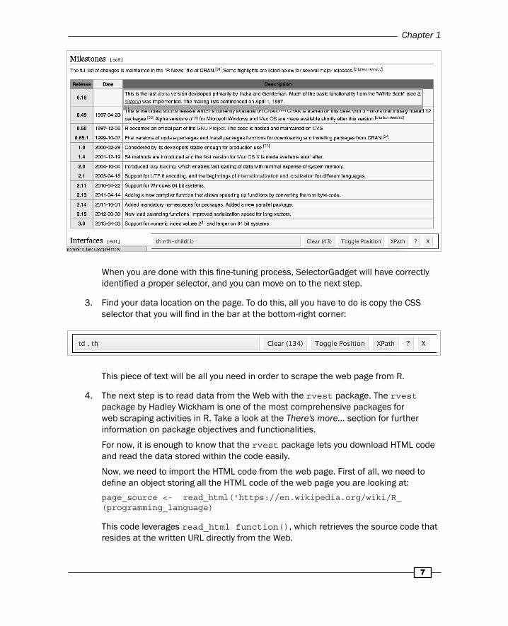
When you are done with this fi ne-tuning process, SelectorGadget will have correctly identifi ed a proper selector, and you can move on to the next step.

3. Find your data location on the page. To do this, all you have to do is copy the CSS selector that you will fi nd in the bar at the bottom-right corner:

This piece of text will be all you need in order to scrape the web page from R.

4. The next step is to read data from the Web with the rvest package. The rvest package by Hadley Wickham is one of the most comprehensive packages for web scraping activities in R. Take a look at the There's more... section for further information on package objectives and functionalities.

For now, it is enough to know that the rvest package lets you download HTML code and read the data stored within the code easily.

Now, we need to import the HTML code from the web page. First of all, we need to defi ne an object storing all the HTML code of the web page you are looking at:

page_source <- read_html('https://en.wikipedia.org/wiki/R_(programming_language)

This code leverages read_html function(), which retrieves the source code that resides at the written URL directly from the Web.

Acquiring Data for Your Project

8

5. Next, we will select the defi ned blocks. Once you have got your HTML code, it is time to extract the part of the code you are interested in. This is done using the html_nodes() function, which is passed as an argument in the CSS selector and retrieved using SelectorGadget. This will result in a line of code similar to the following:

version_block <- html_nodes(page_source,".wikitable th , .wikitable td")

As you can imagine, this code extracts all the content of the selected nodes, including HTML tags.

The HTML language

HyperText Markup Language (HTML) is a markup language that is used to define the format of web pages.

The basic idea behind HTML is to structure the web page into a format with a head and body, each of which contains a variable number of tags, which can be considered as subcomponents of the structure.

The head is used to store information and components that will not be seen by the user but will affect the web page's behavior, for instance, in a Google Analytics script used for tracking page visits, the body contains all the contents which will be showed to the reader.

Since the HTML code is composed of a nested structure, it is common to compare this structure to a tree, and here, different components are also referred to as nodes.

Printing out the version_block object, you will obtain a result similar to the following:

print(version_block)

{xml_nodeset (45)} [1] <th>Release</th> [2] <th>Date</th> [3] <th>Description</th> [4] <th>0.16</th> [5] <td/> [6] <td>This is the last <a href="/wiki/Alpha_test" title="Alpha test" class="mw-redirect">alp ... [7] <th>0.49</th> [8] <td style="white-space:nowrap;">1997-04-23</td> [9] <td>This is the oldest available <a href="/wiki/Source_code" title="Source code">source</a ...[10] <th>0.60</th>[11] <td>1997-12-05</td>[12] <td>R becomes an official part of the <a href="/wiki/GNU_Project" title="GNU Project">GNU ...

Chapter 1

9

[13] <th>1.0</th>[14] <td>2000-02-29</td>[15] <td>Considered by its developers stable enough for production use.<sup id="cite_ref-35" cl ...[16] <th>1.4</th>[17] <td>2001-12-19</td>[18] <td>S4 methods are introduced and the first version for <a href="/wiki/Mac_OS_X" title="Ma ...[19] <th>2.0</th>[20] <td>2004-10-04</td>

This result is not exactly what you are looking for if you are going to work with this data. However, you don't have to worry about that since we are going to give your text a better shape in the very next step.

6. In order to obtain a readable and actionable format, we need one more step: extracting text from HTML tags.

This can be done using the html_text() function, which will result in a list containing all the text present within the HTML tags:

content <- html_text(version_block)

The fi nal result will be a perfectly workable chunk of text containing the data needed for our analysis:

[1] "Release" [2] "Date" [3] "Description" [4] "0.16" [5] "" [6] "This is the last alpha version developed primarily by Ihaka and Gentleman. Much of the basic functionality from the \"White Book\" (see S history) was implemented. The mailing lists commenced on April 1, 1997." [7] "0.49" [8] "1997-04-23" [9] "This is the oldest available source release, and compiles on a limited number of Unix-like platforms. CRAN is started on this date, with 3 mirrors that initially hosted 12 packages. Alpha versions of R for Microsoft Windows and Mac OS are made available shortly after this version."

Acquiring Data for Your Project

10

[10] "0.60" [11] "1997-12-05" [12] "R becomes an official part of the GNU Project. The code is hosted and maintained on CVS." [13] "1.0" [14] "2000-02-29" [15] "Considered by its developers stable enough for production use.[35]" [16] "1.4" [17] "2001-12-19" [18] "S4 methods are introduced and the first version for Mac OS X is made available soon after." [19] "2.0" [20] "2004-10-04" [21] "Introduced lazy loading, which enables fast loading of data with minimal expense of system memory." [22] "2.1" [23] "2005-04-18" [24] "Support for UTF-8 encoding, and the beginnings of internationalization and localization for different languages." [25] "2.11" [26] "2010-04-22" [27] "Support for Windows 64 bit systems." [28] "2.13" [29] "2011-04-14" [30] "Adding a new compiler function that allows speeding up functions by converting them to byte-code."

Chapter 1

11

[31] "2.14" [32] "2011-10-31" [33] "Added mandatory namespaces for packages. Added a new parallel package." [34] "2.15" [35] "2012-03-30" [36] "New load balancing functions. Improved serialization speed for long vectors." [37] "3.0" [38] "2013-04-03" [39] "Support for numeric index values 231 and larger on 64 bit systems." [40] "3.1" [41] "2014-04-10" [42] "" [43] "3.2" [44] "2015-04-16" [45] ""

There's more...The following are a few useful resources that will help you get the most out of this recipe:

A useful list of HTML tags, to show you how HTML fi les are structured and how to identify code that you need to get from these fi les, is provided at http://www.w3schools.com/tags/tag_code.asp

The blog post from the RStudio guys introducing the rvest package and highlighting some package functionalities can be found at http://blog.rstudio.org/2014/11/24/rvest-easy-web-scraping-with-r/

Acquiring Data for Your Project

12

Accessing an API with RAs we mentioned before, an always increasing proportion of our data resides on the Web and is made available through web APIs.

APIs in computer programming are intended to be APIs, groups of procedures, protocols, and software used for software application building. APIs expose software in terms of input, output, and processes.

Web APIs are developed as an interface between web applications and third parties.

The typical structure of a web API is composed of a set of HTTP request messages that have answers with a predefi ned structure, usually in the XML or JSON format.

A typical use case for API data contains data regarding web and mobile applications, for instance, Google Analytics data or data regarding social networking activities.

The successful web application If This ThenThat (IFTTT), for instance, lets you link together different applications, making them share data with each other and building powerful and customizable workfl ows:

This useful job is done by leveraging the application's API (if you don't know IFTTT, just navigate to https://ifttt.com, and I will see you there).

Chapter 1

13

Using R, it is possible to authenticate and get data from every API that adheres to the OAuth 1 and OAuth 2 standards, which are nowadays the most popular standards (even though opinions about these protocols are changing; refer to this popular post by the OAuth creator Blain Cook at http://hueniverse.com/2012/07/26/oauth-2-0-and-the-road-to-hell/). Moreover, specifi c packages have been developed for a lot of APIs.

This recipe shows how to access custom APIs and leverage packages developed for specifi c APIs.

In the There's more... section, suggestions are given on how to develop custom functions for frequently used APIs.

Getting readyThe rvest package, once again a product of our benefactor Hadley Whickham, provides a complete set of functionalities for sending and receiving data through the HTTP protocol on the Web. Take a look at the quick-start guide hosted on GitHub to get a feeling of rvest functionalities (https://github.com/hadley/rvest).

Among those functionalities, functions for dealing with APIs are provided as well.

Both OAuth 1.0 and OAuth 2.0 interfaces are implemented, making this package really useful when working with APIs.

Let's look at how to get data from the GitHub API. By changing small sections, I will point out how you can apply it to whatever API you are interested in.

Let's now actually install the rvest package:

install.packages("rvest")library(rvest)

How to do it…1. The fi rst step to connect with the API is to defi ne the API endpoint. Specifi cations for

the endpoint are usually given within the API documentation. For instance, GitHub gives this kind of information at http://developer.github.com/v3/oauth/.

In order to set the endpoint information, we are going to use the oauth_endpoint() function, which requires us to set the following arguments:

request: This is the URL that is required for the initial unauthenticated token. This is deprecated for OAuth 2.0, so you can leave it NULL in this case, since the GitHub API is based on this protocol.

authorize: This is the URL where it is possible to gain authorization for the given client.

Acquiring Data for Your Project

14

access: This is the URL where the exchange for an authenticated token is made.

base_url: This is the API URL on which other URLs (that is, the URLs containing requests for data) will be built upon.

In the GitHub example, this will translate to the following line of code:

github_api <- oauth_endpoint(request = NULL, authorize = "https://github.com/login/oauth/authorize", access = "https://github.com/login/oauth/access_token", base_url = "https://github.com/login/oauth")

2. Create an application to get a key and secret token. Moving on with our GitHub example, in order to create an application, you will have to navigate to https://github.com/settings/applications/new (assuming that you are already authenticated on GitHub).

Be aware that no particular URL is needed as the homepage URL, but a specifi c URL is required as the authorization callback URL.

This is the URL that the API will redirect to after the method invocation is done.

As you would expect, since we want to establish a connection from GitHub to our local PC, you will have to redirect the API to your machine, setting the Authorization callback URL to http://localhost:1410.

After creating your application, you can get back to your R session to establish a connection with it and get your data.

3. After getting back to your R session, you now have to set your OAuth credentials through the oaut_app() and oauth2.0_token() functions and establish a connection with the API, as shown in the following code snippet:

app <- oauth_app("your_app_name", key = "your_app_key", secret = "your_app_secret") API_token <- oauth2.0_token(github_api,app)

4. This is where you actually use the API to get data from your web-based software. Continuing on with our GitHub-based example, let's request some information about API rate limits:

request <- GET("https://api.github.com/rate_limit", config(token = API_token))

Chapter 1

15

How it works...Be aware that this step will be required both for OAuth 1.0 and OAuth 2.0 APIs, as the difference between them is only the absence of a request URL, as we noted earlier.

Endpoints for popular APIs

The httr package comes with a set of endpoints that are already implemented for popular APIs, and specifi cally for the following websites:

LinkedIn Twitter Vimeo Google Facebook

GitHub

For these APIs, you can substitute the call to oauth_endpoint() with a call to the oauth_endpoints() function, for instance:

oauth_endpoints("github")

The core feature of the OAuth protocol is to secure authentication. This is then provided on the client side through a key and secret token, which are to be kept private.The typical way to get a key and a secret token to access an API involves creating an app within the service providing the API.

The callback URL

Within the web API domain, a callback URL is the URL that is called by the API after the answer is given to the request. A typical example of a callback URL is the URL of the page navigated to after completing an online purchase.

In this example, when we fi nish at the checkout on the online store, an API call is made to the payment circuit provider.

After completing the payment operation, the API will navigate again to the online store at the callback URL, usually to a thank you page.

There's more...You can also write custom functions to handle APIs. When frequently dealing with a particular API, it can be useful to defi ne a set of custom functions in order to make it easier to interact with.

Acquiring Data for Your Project

16

Basically, the interaction with an API can be summarized with the following three categories:

Authentication

Getting content from the API

Posting content to the API

Authentication can be handled by leveraging the HTTR package's authenticate() function and writing a function as follows:

api_auth function (path = "api_path", password){authenticate(user = path, password)}

You can get the content from the API through the get function of the httr package:

api_get <- function(path = "api_path",password){auth <- api_auth(path, password )request <- GET("https://api.com", path = path, auth)

}

Posting content will be done in a similar way through the POST function:

api_post <- function(Path, post_body, path = "api_path",password){auth <- api_auth(pat) stopifnot(is.list(body)) body_json <- jsonlite::toJSON(body) request <- POST("https://api.application.com", path = path, body = body_json, auth, post, ...) }

Getting data from Twitter with the twitteR package

Twitter is an unbeatable source of data for nearly every kind of data-driven problem.

If my words are not enough to convince you, and I think they shouldn't be, you can always perform a quick search on Google, for instance, text analytics with Twitter, and read the over 30 million results to be sure.

This should not surprise you, given Google's huge and word-spreaded base of users together with the relative structure and richness of metadata of content on the platform, which makes this social network a place to go when talking about data analysis projects, especially those involving sentiment analysis and customer segmentations.

R comes with a really well-developed package named twitteR, developed by Jeff Gentry, which offers a function for nearly every functionality made available by Twitter through the API. The following recipe covers the typical use of the package: getting tweets related to a topic.

Chapter 1

17

Getting readyFirst of all, we have to install our great twitteR package by running the following code:

install.packages("twitteR")library(twitter)

How to do it…1. As seen with the general procedure, in order to access the Twitter API, you will need

to create a new application. This link (assuming you are already logged in to Twitter) will do the job: https://apps.twitter.com/app/new.

Feel free to give whatever name, description, and website to your app that you want. The callback URL can be also left blank.

After creating the app, you will have access to an API key and an API secret, namely Consumer Key and Consumer Secret, in the Keys and Access Tokens tab in your app settings.

Below the section containing these tokens, you will fi nd a section called Your Access Token. These tokens are required in order to let the app perform actions on your account's behalf. For instance, you may be willing to send direct messages to all new followers and could therefore write an app to do that automatically.

Keep a note of these tokens as well, since you will need them to set up your connection within R.

2. Then, we will get access to the API from R. In order to authenticate your app and use it to retrieve data from Twitter, you will just need to run a line of code, specifi cally, the setup_twitter_oauth() function, by passing the following arguments:

consumer_key

consumer_token

access_token

access_secret

You can get these tokens from your app settings:

setup_twitter_oauth(consumer_key = "consumer_key", consumer_secret = "consumer_secret", access_token = "access_token", access_secret = "access_secret")

Acquiring Data for Your Project

18

3. Now, we will query Twitter and store the resulting data. We are fi nally ready for the core part: getting data from Twitter. Since we are looking for tweets pertaining to a specifi c topic, we are going to use the searchTwitter() function. This function allows you to specify a good number of parameters besides the search string. You can defi ne the following:

n : This is the number of tweets to be downloaded.

lang: This is the language specified with the ISO 639-1 code. You can find a partial list of this code at https://en.wikipedia.org/wiki/List_of_ISO_639-1_codes.

since – until: These are time parameters that define a range of time, where dates are expressed as YYYY-MM-DD, for instance, 2012-05-12.

locale: This specifies the geocode, expressed as latitude, longitude and radius, either in miles or kilometers, for example, 38.481157,-130.500342,1 mi.

sinceID – maxID: This is the account ID range.

resultType: This is used to filter results based on popularity. Possible values are 'mixed', 'recent', and 'popular'.

retryOnRateLimit: This is the number that defines how many times the query will be retried if the API rate limit is reached.

Supposing that we are interested in tweets regarding data science with R; we run the following function:

tweet_list <- searchTwitter('data science with R', n = 450)

Performing a character-wise search with twitteR

Searching Twitter for a specific sequence of characters is possible by submitting a query surrounded by double quotes, for instance, "data science with R". Consequently, if you are looking to retrieve tweets in R corresponding to a specific sequence of characters, you will have to submit and run a line of code similar to the following:

tweet_list <- searchTwitter('data science with R', n = 450)

tweet_list will be a list of the fi rst 450 tweets resulting from the given query.

Be aware that since n is the maximum number of tweets retrievable, you may retrieve a smaller number of tweets, if for the given query the number or result is smaller than n.

Chapter 1

19

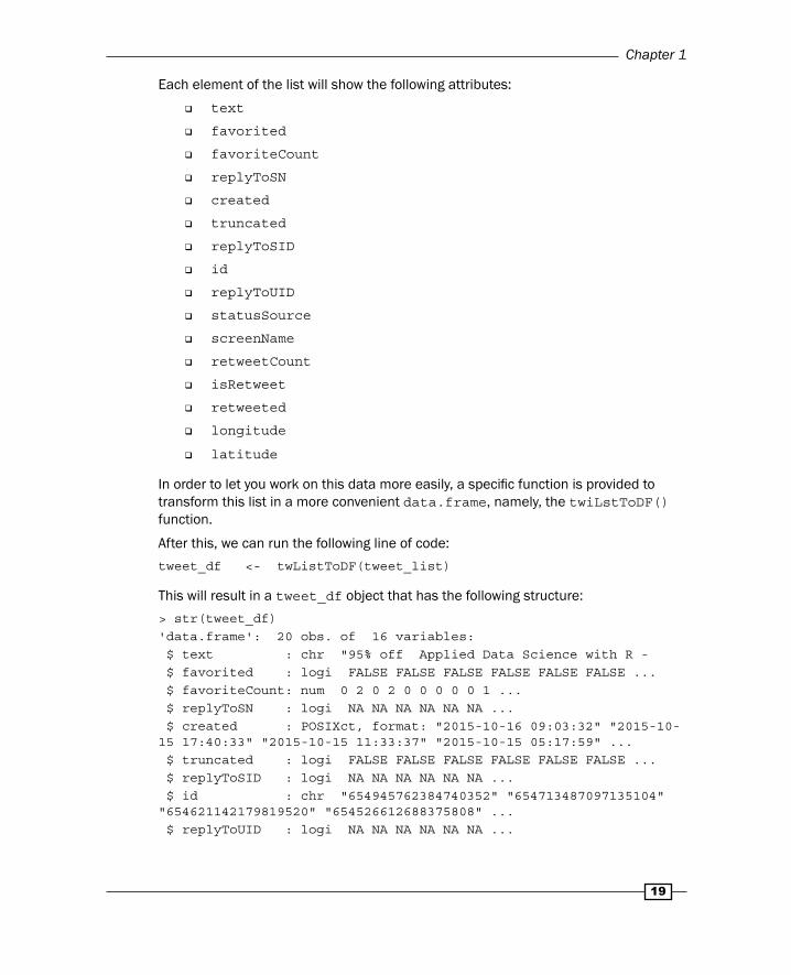
Each element of the list will show the following attributes:

text

favorited

favoriteCount

replyToSN

created

truncated

replyToSID

id

replyToUID

statusSource

screenName

retweetCount

isRetweet

retweeted

longitude

latitude

In order to let you work on this data more easily, a specifi c function is provided to transform this list in a more convenient data.frame, namely, the twiLstToDF() function.

After this, we can run the following line of code:

tweet_df <- twListToDF(tweet_list)

This will result in a tweet_df object that has the following structure:

> str(tweet_df)'data.frame': 20 obs. of 16 variables: $ text : chr "95% off Applied Data Science with R - $ favorited : logi FALSE FALSE FALSE FALSE FALSE FALSE ... $ favoriteCount: num 0 2 0 2 0 0 0 0 0 1 ... $ replyToSN : logi NA NA NA NA NA NA ... $ created : POSIXct, format: "2015-10-16 09:03:32" "2015-10-15 17:40:33" "2015-10-15 11:33:37" "2015-10-15 05:17:59" ... $ truncated : logi FALSE FALSE FALSE FALSE FALSE FALSE ... $ replyToSID : logi NA NA NA NA NA NA ... $ id : chr "654945762384740352" "654713487097135104" "654621142179819520" "654526612688375808" ... $ replyToUID : logi NA NA NA NA NA NA ...

Acquiring Data for Your Project

20

$ statusSource : chr "<a href=\"http://learnviral.com/\" rel=\"nofollow\">Learn Viral</a>" "<a href=\"https://about.twitter.com/products/tweetdeck\" rel=\"nofollow\">TweetDeck</a>" "<a href=\"http://not.yet/\" rel=\"nofollow\">final one kk</a>" "<a href=\"http://twitter.com\" rel=\"nofollow\">Twitter Web Client</a>" ... $ screenName : chr "Learn_Viral" "WinVectorLLC" "retweetjava" "verystrongjoe" ... $ retweetCount : num 0 0 1 1 0 0 0 2 2 2 ... $ isRetweet : logi FALSE FALSE TRUE FALSE FALSE FALSE ... $ retweeted : logi FALSE FALSE FALSE FALSE FALSE FALSE ... $ longitude : logi NA NA NA NA NA NA ... $ latitude : logi NA NA NA NA NA NA ...

After sending you to the data visualization section for advanced techniques, we will now quickly visualize the retweet distribution of our tweets, leveraging the base R hist() function:

hist(tweet_df$retweetCount)

This code will result in a histogram that has the x axis as the number of retweets and the y axis as the frequency of those numbers:

There's more...As stated in the offi cial Twitter documentation, particularly at https://dev.twitter.com/rest/public/rate-limits, there is a limit to the number of tweets you can retrieve within a certain period of time, and this limit is set to 450 every 15 minutes.

Chapter 1

21

However, what if you are engaged in a really sensible job and you want to base your work on a signifi cant number of tweets? Should you set the n argument of searchTwitter() to 450 and wait for 15—everlasting—minutes? Not quite, the twitteR package provides a convenient way to overcome this limit through the register_db_backend(), register_sqlite_backend(), and register_mysql_bakend() functions. These functions allow you to create a connection with the named type of databases, passing the database name, path, username, and password as arguments, as you can see in the following example:

register_mysql_backend("db_name", "host","user","password")

You can now leverage the search_twitter_and_store function, which stores the search results in the connected database. The main feature of this function is the retryOnRateLimit argument, which lets you specify the number of tries to be performed by the code once the API limit is reached. Setting this limit to a convenient level will likely let you pass the 15-minutes interval:

tweets_db = search_twitter_and_store("data science R", retryOnRateLimit = 20)

Retrieving stored data will now just require you to run the following code:

from_db = load_tweets_db()

Getting data from Facebook with the Rfacebook package

The Rfacebook package, developed and maintained by Pablo Barberá, lets you easily establish and take advantage of Facebook's API thanks to a series of functions.

As we did for the twitteR package, we are going to establish a connection with the API and retrieve posts pertaining to a given keyword.

Getting readyThis recipe will mainly be based on functions from the Rfacebok package. Therefore, we need to install and load this package in our environment:

install.packages("Rfacebook")library(Rfacebook)

Acquiring Data for Your Project

22

How to do it...1. In order to leverage an API's functionalities, we fi rst have to create an application

in our Facebook profi le. Navigating to the following URL will let you create an app (assuming you are already logged in to Facebook): https://developers.facebook.com.

After skipping the quick start (the button on the upper-right corner), you can see the settings of your app and take note of app_id and app_secret, which you will need in order to establish a connection with the app.

2. After installing and loading the Rfacebook package, you will easily be able to establish a connection by running the fbOAuth() function as follows:

fb_connection <- fbOauth(app_id = "your_app_id", app_secret = "your_app_secret")fb_connection

Running the last line of code will result in a console prompt, as shown in the following lines of code:

copy and paste into site URL on Facebook App Settings: http://localhost:1410/ When done press any key to continue

Following this prompt, you will have to copy the URL and go to your Facebook app settings.

Once there, you will have to select the Settings tab and create a new platform through the + Add Platform control. In the form, which will prompt you after clicking this control, you should fi nd a fi eld named Site Url. In this fi eld, you will have to paste the copied URL.

Close the process by clicking on the Save Changes button.

At this point, a browser window will open up and ask you to allow access permission from the app to your profi le. After allowing this permission, the R console will print out the following code snippet:

Authentication complete

Authentication successful.

3. To test our API connection, we are going to search Facebook for posts related to data science with R and save the results within data.frame for further analysis.

Among other useful functions, Rfacebook provides the searchPages() function, which as you would expect, allows you to search the social network for pages mentioning a given string.

Chapter 1

23

Different from the searchTwitter function, this function will not let you specify a lot of arguments:

string: This is the query string

token: This is the valid OAuth token created with the fbOAuth() function

n: This is the maximum number of posts to be retrieved

The Unix timestamp

The Unix timestamp is a time-tracking system originally developed for the Unix OS. Technically, the Unix timestamp x expresses the number of seconds elapsed since the Unix Epoch (January 1, 1970 UTC) and the timestamp.

To search for data science with R, you will have to run the following line of code:

pages ← searchPages('data science with R',fb_connection)

This will result in data.frame storing all the pages retrieved along with the data concerning them.

As seen for the twitteR package, we can take a quick look at the like distribution, leveraging the base R hist() function:

hist(pages$likes)

This will result in a plot similar to the following:

Refer to the data visualization section for further recipes on data visualization.

Acquiring Data for Your Project

24

Getting data from Google AnalyticsGoogle Analytics is a powerful analytics solution that gives you really detailed insights into how your online content is performing. However, besides a tabular format and a data visualization tool, no other instruments are available to model your data and gain more powerful insights.

This is where R comes to help, and this is why the RGoogleAnalytics package was developed: to provide a convenient way to extract data from Google Analytics into an R environment.

As an example, we will import data from Google Analytics into R regarding the daily bounce rate for a website in a given time range.

Getting readyAs a preliminary step, we are going to install and load the RGoogleAnalytics package:

install.packages("RGoogeAnalytics")library(RGoogleAnalytics)

How to do it...1. The fi rst step that is required to get data from Google Analytics is to create a Google

Analytics application.

This can be easily obtained from (assuming that you are already logged in to Google Analytics) https://console.developers.google.com/apis.

After creating a new project, you will see a dashboard with a left menu containing among others the APIs & auth section, with the APIs subsection.

After selecting this section, you will see a list of available APIs, and among these, at the bottom-left corner of the page, there will be the Advertising APIs with the Analytics API within it:

Chapter 1

25

After enabling the API, you will have to go back to the APIs & auth section and select the Credentials subsection.

In this section, you will have to add an OAuth client ID, select Other, and assign a name to your app:

After doing that and selecting the Create button, you will be prompted with a window showing your app ID and secret. Take note of them, as you will need them to access the analytics API from R.

Acquiring Data for Your Project

26

2. In order to authenticate on the API, we will leverage the Auth() function, providing the annotated ID and secret:

ga_token ← Auth(client.id = "the_ID", client.secret = "the_secret")

At this point, a browser window will open up and ask you to allow access permission from the app to your Google Analytics account.

After you allow access, the R console will print out the following:

Authentication complete

3. This last step basically requires you to shape a proper query and submit it through the connection established in the previous paragraphs. A Google Analytics query can be easily built, leveraging the powerful Google Query explorer which can be found at https://ga-dev-tools.appspot.com/query-explorer/.

This web tool lets you experiment with query parameters and defi ne your query before submitting the request from your code.

The basic fi elds that are mandatory in order to execute a query are as follows:

The view ID: This is a unique identifier associated with your Google Analytics property. This ID will automatically show up within Google Query Explorer.

Start-date and end-date: This is the start and end date in the form YYYY-MM-DD, for example, 2012-05-12.

Metrics: This refers to the ratios and numbers computed from the data related to visits within the date range. You can find the metrics code in Google Query Explorer.

If you are going to further elaborate your data within your data project, you will probably fi nd it useful to add a date dimension ("ga:date") in order to split your data by date.

Having defi ned your arguments, you will just have to pack them in a list using the init() function, build a query using the QueryBuilder() function, and submit it with the GetReportData() function:

query_parameters <- Init(start.date = "2015-01-01", end.date = "2015-06-30", metrics = "ga:sessions, ga:bounceRate", dimensions = "ga:date", table.id = "ga:33093633")ga_query <- QueryBuilder(query_parameters)ga_df <- GetReportData(ga_query, ga_token)

The fi rst representation of this data could be a simple plot of data that will result in a representation of the bounce rate for each day from the start date to the end date:

plot(ga_df)

Chapter 1

27

There's more...Google Analytics is a complete and always-growing set of tools for performing web analytics tasks. If you are facing a project involving the use of this platform, I would defi nitely suggest that you take the time to go through the offi cial tutorial from Google at https://analyticsacademy.withgoogle.com.

This complete set of tutorials will introduce you to the fundamental logic and assumptions of the platform, giving you a solid foundation for any of the following analysis.

Loading your data into R with rio packagesThe rio package is a relatively recent R package, developed by Thomas J. Leeper, which makes data import and export in R painless and quick.

This objective is mainly reached when rio makes assumptions about the fi le format. This means that the rio package guesses the format of the fi le you are trying to import and consequently applies import functions appropriate to that format.

All of this is done behind the scenes, and the user is just required to run the import() function.

As Leeper often states when talking about the package: "it just works."

One of the great results you can obtain by employing this package is streamlining workfl ows involving different development and productivity tools.

For instance, it is possible to produce tables directly into SAS and make them available to the R environment without any particular export procedure in SAS, we can directly acquire data in R as it is produced, or input into an Excel spreadsheet.

Getting readyAs you would expect, we fi rst need to install and load the rio package:

install.packages("rio")library(rio)

In the following example, we are going to import our well-known world_gdp_data dataset from a local .csv fi le.

Acquiring Data for Your Project

28

How to do it...1. The fi rst step is to import the dataset using the import() function:

messy_gdp ← import("world_gdp_data.csv")

2. Then, we visualize the result with the RStudio viewer:

View(messy_gdp)

How it works...We fi rst import the dataset using the import() function. To understand the structure of the import() function, we can leverage a useful behavior of the R console: putting a function name without parentheses and running the command will result in the printing of all the function defi nitions.

Running the import on the R console will produce the following output:

function (file, format, setclass, ...) { if (missing(format)) fmt <- get_ext(file) else fmt <- tolower(format) if (grepl("^http.*://", file)) { temp_file <- tempfile(fileext = fmt) on.exit(unlink(temp_file)) curl_download(file, temp_file, mode = "wb") file <- temp_file } x <- switch(fmt, r = dget(file = file), tsv = import.delim(file = file, sep = "\t", ...), txt = import.delim(file = file, sep = "\t", ...), fwf = import.fwf(file = file, ...), rds = readRDS(file = file, ...), csv = import.delim(file = file, sep = ",", ...), csv2 = import.delim(file = file, sep = ";", dec = ",", ...), psv = import.delim(file = file, sep = "|", ...), rdata = import.rdata(file = file, ...), dta = import.dta(file = file, ...), dbf = read.dbf(file = file, ...), dif = read.DIF(file = file, ...), sav = import.sav(file = file, ...), por = read_por(path = file), sas7bdat = read_sas(b7dat = file, ...), xpt = read.xport(file = file),

Chapter 1

29

mtp = read.mtp(file = file, ...), syd = read.systat(file = file, to.data.frame = TRUE), json = fromJSON(txt = file, ...), rec = read.epiinfo(file = file, ...), arff = read.arff(file = file), xls = read_excel(path = file, ...), xlsx = import.xlsx(file = file, ...), fortran = import.fortran(file = file, ...), zip = import.zip(file = file, ...), tar = import.tar(file = file, ...), ods = import.ods(file = file, ...), xml = import.xml(file = file, ...), clipboard = import.clipboard(...), gnumeric = stop(stop_for_import(fmt)), jpg = stop(stop_for_import(fmt)), png = stop(stop_for_import(fmt)), bmp = stop(stop_for_import(fmt)), tiff = stop(stop_for_import(fmt)), sss = stop(stop_for_import(fmt)), sdmx = stop(stop_for_import(fmt)), matlab = stop(stop_for_import(fmt)), gexf = stop(stop_for_import(fmt)), npy = stop(stop_for_import(fmt)), stop("Unrecognized file format")) if (missing(setclass)) { return(set_class(x)) } else { a <- list(...) if ("data.table" %in% names(a) && isTRUE(a[["data.table"]])) setclass <- "data.table" return(set_class(x, class = setclass)) }}

As you can see, the fi rst task performed by the import() function calls the get_ext() function, which basically retrieves the extension from the fi lename.

Once the fi le format is clear, the import() function looks for the right subimport function to be used and returns the result of this function.

Next, we visualize the result with the RStudio viewer. One of the most powerful RStudio tools is the data viewer, which lets you get a spreadsheet-like view of your data.frame objects. With RStudio 0.99, this tool got even more powerful, removing the previous 1000-row limit and adding the ability to fi lter and format your data in the correct order.

When using this viewer, you should be aware that all fi ltering and ordering activities will not affect the original data.frame object you are visualizing.

Acquiring Data for Your Project

30

There's more...As fully illustrated within the Rio vignette (which can be found at https://cran.r-project.org/web/packages/rio/vignettes/rio.html), the following formats are supported for import and export:

Format Import Export

Tab-separated data (.tsv) Yes Yes

Comma-separated data (.csv) Yes Yes

CSVY (CSV + YAML metadata header) (.csvy) Yes Yes

Pipe-separated data (.psv) Yes Yes

Fixed-width format data (.fwf) Yes Yes

Serialized R objects (.rds) Yes Yes

Saved R objects (.RData) Yes Yes

JSON (.json) Yes Yes

YAML (.yml) Yes Yes

Stata (.dta) Yes Yes

SPSS and SPSS portable Yes (.sav and .por) Yes (.sav only)

XBASE database files (.dbf) Yes Yes

Excel (.xls) Yes

Excel (.xlsx) Yes Yes

Weka Attribute-Relation File Format (.arff) Yes Yes

R syntax (.R) Yes Yes

Shallow XML documents (.xml) Yes Yes

SAS (.sas7bdat) Yes

SAS XPORT (.xpt) Yes

Minitab (.mtp) Yes

Epiinfo (.rec) Yes

Systat (.syd) Yes

Data Interchange Format (.dif) Yes

OpenDocument Spreadsheet (.ods) Yes

Fortran data (no recognized extension) Yes

Google Sheets Yes

Clipboard (default is .tsv)

Chapter 1

31

Since Rio is still a growing package, I strongly suggest that you follow its development on its GitHub repository, where you will easily fi nd out when new formats are added, at https://github.com/leeper/rio.

Converting fi le formats using the rio package

As we saw in the previous recipe, Rio is an R package developed by Thomas J. Leeper which makes the import and export of data really easy. You can refer to the previous recipe for more on its core functionalities and logic.

Besides the import() and export() functions, Rio also offers a really well-conceived and straightforward fi le conversion facility through the convert() function, which we are going to leverage in this recipe.

Getting readyF irst of all, we need to install and make the rio package available by running the following code:

install.packages("rio")library(rio)

In the following example, we are going to import the world_gdp_data dataset from a local .csv fi le. This dataset is provided within the RStudio project related to this book, in the data folder.

You can download it by authenticating your account at http://packtpub.com.

How to do it...1. The fi rst step is to convert the fi le from the .csv format to the .json format:

convert("world_gdp_data.csv", "world_gdp_data.json")

This will create a new fi le without removing the original one.

2. The next step is to remove the original fi le:

file.remove("world_gdp_data.csv")

Acquiring Data for Your Project

32

There's more...As fully illustrated within the Rio vignette (which you can fi nd at https://cran.r-project.org/web/packages/rio/vignettes/rio.html), the following formats are supported for import and export:

Format Import Export

Tab-separated data (.tsv) Yes Yes

Comma-separated data (.csv) Yes Yes

CSVY (CSV + YAML metadata header) (.csvy) Yes Yes

Pipe-separated data (.psv) Yes Yes

Fixed-width format data (.fwf) Yes Yes

Serialized R objects (.rds) Yes Yes

Saved R objects (.RData) Yes Yes

JSON (.json) Yes Yes

YAML (.yml) Yes Yes

Stata (.dta) Yes Yes

SPSS and SPSS portable Yes (.sav and .por) Yes (.sav only)

XBASE database files (.dbf) Yes Yes

Excel (.xls) Yes

Excel (.xlsx) Yes Yes

Weka Attribute-Relation File Format (.arff) Yes Yes

R syntax (.r) Yes Yes

Shallow XML documents (.xml) Yes Yes

SAS (.sas7bdat) Yes

SAS XPORT (.xpt) Yes

Minitab (.mtp) Yes

Epiinfo (.rec) Yes

Systat (.syd) Yes

Data Interchange Format (.dif) Yes

OpenDocument Spreadsheet (.ods) Yes

Fortran data (no recognized extension) Yes

Google Sheets Yes

Clipboard (default is .tsv)

Since rio is still a growing package, I strongly suggest that you follow its development on its GitHub repository, where you will easily fi nd out when new formats are added, at https://github.com/leeper/rio.

Where to buy this book You can buy RStudio for R Statistical Computing Cookbook from the

Packt Publishing website.

Alternatively, you can buy the book from Amazon, BN.com, Computer Manuals and most internet

book retailers.

Click here for ordering and shipping details.

www.PacktPub.com

Stay Connected:

Get more information RStudio for R Statistical Computing Cookbook