rp_gub_13_03
DESCRIPTION
adadaTRANSCRIPT

c©2011 by Taejeong Kim 1
Transform
• probability generating function, pgf,for nonnegative integer-valued X
GX(z) := EzX =∑∞
n=0 znpX(n)
Defined in terms of expectation, it is more fundamental thanpmf in describing a random variable.
GX(z−1) is the z-transform of pX(n).
P (X = k) = pX(k) = G(k)X (z)|z=0/k!
: probability generating property
Y =∑m
i=1 aiXi ⇒ GY (z) = E∏m
i=1 zaiXi
=∏m
i=1 E zaiXi if independent
=∏m
i=1 GXi(zai)
= (GX(z))m if iid and ai = 1

c©2011 by Taejeong Kim 2
Ber(p) GX(z) = 1−p+pz⇒ Bin(n, p) GY (z) = (1−p+pz)n
•moment generating function, mgf, for continuous X
MX(s) := EesX =∫ ∞−∞ esxfX(x)dx
Defined in terms of expectation, it is more fundamental thanpdf in describing a random variable.
MX(−s) is the Laplace transform of fX(x).
When s is a real variable, the mgf may not exist.
EXk = M(k)X (s)|s=0: moment generating property
Y =∑m
i=1 aiXi ⇒ MY (z) = E∏m
i=1 esaiXi
=∏m
i=1 E esaiXi if independent
=∏m
i=1 MXi(ais)
= (MX(s))m if iid and ai = 1

c©2011 by Taejeong Kim 3
exp(λ) MX(s) = λλ−s ⇒ Erl(m,λ) MX(s) =
λλ−s
m
• characteristic function, chf, of X
ϕX(u) := EejuX =
∑ejuxpX(x)
∫ejuxfX(x)dx
Defined in terms of expectation, it is more fundamental thanpmf or pdf in describing a random variable.
ϕX(−u) is the Fourier transform of pX(x) or fX(x).
The chf always exists and fully characterizes the randomvariable.
EXk = ϕ(k)X (u)|u=0/j
k: moment generating property
ϕX(0) = 1, |ϕX(u)| ≤ 1
The chf is conjugate symmetric (self adjoint, Hermitian).
real symmetric pmf or pdf ⇒ real symmetric chf

c©2011 by Taejeong Kim 4
Gaussian chf: X ∼ N(m,σ2)
ϕX(u) = exp
jmu− σ2u2
2
• joint characteristic function, jchf, of X and Y
ϕXY (u, v) := Eej(uX+vY ) =
∑∑ej(ux+vy)pXY (x, y)
∫ ∫ej(ux+vy)fXY (x, y)dxdy
ϕXY (−u, −v) is the 2-d Fourier transform.
EXkY l = ϕ(k)(l)XY (u, v)|u=v=0/j
k+l
: moment generating property
ϕXY (0, 0) = 1, |ϕXY (u, v)| ≤ 1
X and Y are independent ⇔ ϕXY (u, v) = ϕX(u)ϕY (v)
It extends to k random variables.

c©2011 by Taejeong Kim 5
Weak law of large numbers, WLLN
• sample mean: Mn := 1n
∑ni=1 Xi
The sample mean is an unbiased estimator of mX if EXi =mX, i = 1, ···, n. That is, EMn = mX.
data samples → probabilistic model → iid random variables→ sample mean
•weak law of large numbers:
X1, · · · , Xk iid, EXi = m, var(Xi) = σ2
EMn = m, var(Mn) = σ2
n
⇒ ∀ ε > 0, limn→∞P (|Mn −m| ≥ ε) = 0
Xi
ppppppppppppppppppppppppppppppppppp
ppppppppppppppppppppppppppppppppppp
M2
M5
M10
proof: P (|Mn −m| ≥ ε) ≤ var(Mn)/ε2
[Chebychev ineq]

c©2011 by Taejeong Kim 6
This type of convergence is called the “convergence in prob-ability”; so we write Mn → m in probability as n →∞.
A stronger convergence called “convergence with probabilityone” or “almost sure convergence” also holds and is referredto as the strong law of large numbers.
pMn(x) gets narrower as n →∞ approaching a single prob-ability mass.1√n
∑ni=1 Xi retains variance as n →∞. → central limit thm

c©2011 by Taejeong Kim 7
Conditional probability of random variables
• conditional pmf, cpmf :
pX|A(x) := P (X = x|A) =P (X = x ∩ A)
P (A)
A = Y = y ⇒ pX|Y (x|y) :=pXY (x, y)
pY (y)
pX|Y Z(x|y, z) = pXY Z(x, y, z)/pY Z(y, z)
pXY |Z(x, y|z) = pXY Z(x, y, z)/pZ(z)

c©2011 by Taejeong Kim 8
• conditional pdf, cpdf :
fX|A(x) := lim∆x→0
P (x < X ≤ x + ∆x|A)
∆x
= lim∆x→0
P (x < X ≤ x + ∆x ∩ A)
∆x p(A)
fX|Y (x|y) :=fXY (x, y)
fY (y)
not defined when the denominator is zero.
point conditioning for continuous Y : If it exists,
P (B|Y = y) := lim∆y→0
P (B ∩ y < Y ≤ y + ∆y)P (y < Y ≤ y + ∆y)
⇒ fX|Y (x|y) = fX|A(x), where A = Y = y

c©2011 by Taejeong Kim 9
fX|Y Z(x|y, z) = fXY Z(x, y, z)/fY Z(y, z)
fXY |Z(x, y|z) = fXY Z(x, y, z)/fZ(z)
Given a conditioning event, the cpmf and cpdf are just like apmf and pdf, respectively.
cpmf and cpdf can be used in discrete-continuous combination.
X , Y indep ⇒
pX|Y (x|y) = pX(x)
fX|Y (x|y) = fX(x)
chain rule:
pXY (x, y) = pX(x)pY |X(y|x)
pX1···Xk(x1, · · · , xk)
= pX1(x1)pX2|X1
(x2|x1) · · · pXk|X1···Xk−1(xk|x1, · · · , xk−1)
pXY |W (x, y|w) = pX|W (x|w)pY |WX(y|w, x)

c©2011 by Taejeong Kim 10
pXY Z|W (x, y, z|w) = pXY |W (x, y|w)pZ|WXY (z|w, x, y)
fXY (x, y) = fX(x)fY |X(y|x)
fX1···Xk(x1, · · · , xk)
= fX1(x1)fX2|X1
(x2|x1) · · · fXk|X1···Xk−1(xk|x1, · · · , xk−1)
fXY |W (x, y|w) = fX|W (x|w)fY |WX(y|w, x)
fXY Z|W (x, y, z|w) = fXY |W (x, y|w)fZ|WXY (z|w, x, y)
total probability law:
pX(x) =∑
y pXY (x, y) =∑
y pX|Y (x|y)pY (y)
P (X ∈ C) =∑
x∈C pX(x) =∑
x∈C [∑
y pXY (x, y)]
=∑
x∈C [∑
y pY (y)pX|Y (x|y)]
=∑
y [∑
x∈C pX|Y (x|y)]pY (y)
=∑
y P (X ∈ C|Y = y)P (Y = y)

c©2011 by Taejeong Kim 11
fX(x) =∫fXY (x, y)dy =
∫fX|Y (x|y)fY (y)dy
P (X ∈ C) =∫
C fX(x)dx =∫
C [∫fXY (x, y)dy]dx
=∫
C [∫fY (y)fX|Y (x|y)dy]dx
=∫[∫
C fX|Y (x|y)dx]fY (y)dy
=∫P (X ∈ C|Y = y)fY (y)dy
substitution law:
P (g(X, Y ) ∈ B|X = x) = P (g(x, Y ) ∈ B|X = x)
= P (g(x, Y ) ∈ B) if X , Y indep
c©2011 by Taejeong Kim 12
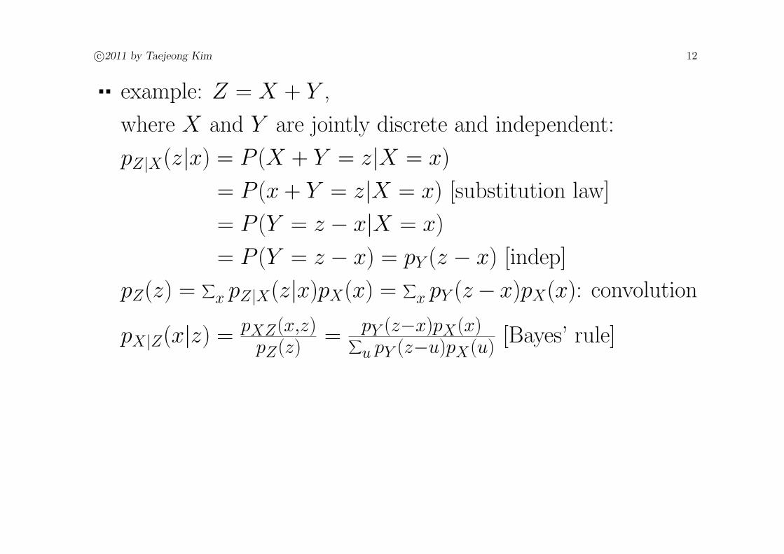
example: Z = X + Y ,
where X and Y are jointly discrete and independent:
pZ|X(z|x) = P (X + Y = z|X = x)
= P (x + Y = z|X = x) [substitution law]
= P (Y = z − x|X = x)
= P (Y = z − x) = pY (z − x) [indep]
pZ(z) =∑
x pZ|X(z|x)pX(x) =∑
x pY (z− x)pX(x): convolution
pX|Z(x|z) = pXZ(x,z)pZ(z)
= pY (z−x)pX(x)∑
u pY (z−u)pX(u)[Bayes’ rule]

c©2011 by Taejeong Kim 13
Similarly, if X and Y are jointly continuous and independent,
fZ|X(z|x) = lim∆→0 P (z < X + Y ≤ z + ∆|X = x)/∆
= lim∆→0 P (z < x + Y ≤ z + ∆|X = x)/∆ [subst]
= lim∆→0 P (z − x < Y ≤ z − x + ∆|X = x)/∆
= lim∆→0 P (z − x < Y ≤ z − x + ∆)/∆ [indep]
= fY (z − x)
fZ(z) =∫fY (z − x)fX(x)dx: convolution
fX|Z(x|z) = fXZ(x,z)
fZ(z)= fY (z−x)fX(x)
∫fY (z−u)fX(u)du
[Bayes’ rule]

c©2011 by Taejeong Kim 14
conditional independence:
X and Y are conditionally independent given Z:
pXY |Z(x, y|z) = pX|Z(x|z)pY |Z(y|z) jointly discfXY |Z(x, y|z) = fX|Z(x|z)fY |Z(y|z) jointly cont
X and Y are independent.6⇒ X and Y are conditionally independent given Z.
example: X and Y are independent Bernoulli rvs.
Z = X + Y
X and Y are conditionally independent given Z.6⇒ X and Y are independent.
example: U , V , and Z are independent Bernoulli rvs.
X = U + Z, Y = V + Z

c©2011 by Taejeong Kim 15
Decision Problem
decision problem: observe Y (effect or result), decide X(cause)among a finite number of choices, given pY |X(y|x) or pXY (x, y)
likelihood: pY |X(y|x)
a posteriori probability: pX|Y (x|y)
maximum likelihood, ML, decision:
decide X = x based on the observation y such that
x = max−1(pY |X(y|x))
maximum a posteriori probability, MAP, decision:
decide X = x based on the observation y such that
x = max−1(pX|Y (x|y))
Which is more meaningful?

c©2011 by Taejeong Kim 16
max−1x (pX|Y (x|y)) = max−1
x (pXY (x, y)/pY (y))
= max−1x (pXY (x, y))
= max−1x (pY |X(y|x)pX(x))
⇒ When pX(x) is uniform or unknown, MAP=ML.
A set of parallel statements hold for continuous Y .
example:x 1 2 3
pX(x) 0.2 0.3 0.5
pY |X(y|x) x = 1 x = 2 x = 3y = 1 0.2 0.1 0.1y = 2 0.8 0.9 0.9
⇒pX|Y (x|y) x = 1 x = 2 x = 3
y = 1 1/3 1/4 5/12y = 2 2/11 27/88 45/88
observation ML MAPy = 1 x = 1 x = 3y = 2 x = 2 or 3 x = 3

c©2011 by Taejeong Kim 17
When decision is among two choices, 0 and 1 ⇒ detection(detection hypotheses: H0 target non-exists, H1 target exists)
ML:pY |X(y|1)
pY |X(y|0)
<> 1
MAP:pY |X(y|1)
pY |X(y|0)
<>
pX(0)
pX(1)
: likelihood ratio test
When X takes an infinite number of values, it becomes anestimation problem: observe Y , estimate X as a functiong(Y ), given fY |X(y|x) or fXY (x, y)

c©2011 by Taejeong Kim 18
maximum likelihood, ML, estimation:
g(Y ) = max−1x (fY |X(Y |x))
maximum a posteriori probability, MAP, estimation:
g(Y ) = max−1x (fX|Y (x|Y )) = max−1
x (fY |X(Y |x)fX(x))
⇒ When fX(x) is uniform or unknown, MAP=ML.
A set of parallel statements hold for discrete Y .
Note that our probabilistic estimation is different from statis-tical parameter estimation (chapter 6, Gubner).
probabilistic estimation statistical estimationobservation random, single random, multiple
target random variable deterministic parameter

c©2011 by Taejeong Kim 19
Though we discussed only ML and MAP rules in relation toconditional probabilities, there are other rules:
minimum probability of error
minimum mean-squared-error, mmse
Bayes’
Neymann-Pearson, NP
Under certain conditions, some of these become equivalent.

c©2011 by Taejeong Kim 20
Conditional expectation
conditional expectation given an event
E(X|A) :=
∑x xpX|A(x)
∫
x xfX|A(x)dxfor an event A.
This depends on the event A.
E(X|Y = y) :=
∑x xpX|Y (x|y)
∫xfX|Y (x|y)dx
This is a function of y [for the given pXY (x, y) or fXY (x, y)].
E(g(X)|Y = y) =
∑x g(x)pX|Y (x|y)
∫g(x)fX|Y (x|y)dx
substitution law:
E(g(X, Y )|Y = y) = E(g(X, y)|Y = y)
= Eg(X, y) if X ,Y are indep.

c©2011 by Taejeong Kim 21
E(g(X)h(Y )|Y = y) = E(g(X)h(y)|Y = y)
= h(y)E(g(X)|Y = y)
= h(y)Eg(X) if X ,Y are indep.
total probability law:
EX =∑
x xpX(x) =∑
x x[∑
y pY (y)pX|Y (x|y)] [j disc case]
=∑
y pY (y)[∑
x xpX|Y (x|y)]
=∑
y E(X|Y = y)pY (y)
This is two-step averaging, as, in averaging a matrix of num-bers, averaging row-wise first then column-wise.
Eg(X) =∑
y E[g(X)|Y = y]pY (y)
Eg(X,Y ) =∑
y E[g(X, y)|Y = y]pY (y)

c©2011 by Taejeong Kim 22
EX =∫xfX(x)dx =
∫x (
∫fY (y)fX|Y (x|y)dy)dx [j cont case]
=∫fY (y)(
∫xfX|Y (x|y)dx)dy
=∫E(X|Y = y)fY (y)dy
Eg(X) =∫E(g(X)|Y = y)fY (y)dy
Eg(X,Y ) =∫E(g(X, y)|Y = y)fY (y)dy
conditional expectation E(X|Y )
E(X|Y = y) = q(y) ⇒ E(X|Y ) := q(Y )
E(X|Y ) is a function of Y and hence a random variable.
If q is one-to-one, P [E(X|Y ) = E(X|Y = y)] = P (Y = y).
For each y, E(X|Y ) is X averaged over the event whereY = y.

c©2011 by Taejeong Kim 23
example: Roll a die until we get a 6.
Y : the total number of rolls; X : the total number of 1’s
pX|Y (x|y) ∼ bin(y−1, 1/5)
E(X|Y = y) =∑
x xpX|Y (x|y) = y−15
This is a function of y, and call it q(y).
We now consider q(Y ) = Y−15
, a new random variable denoted
by E(X|Y ).
X
Y
-
6
¥¥¥¥¥¥¥¥¥¥¥¥¥¥¥
uu uu u uu u u uu u u u uu u u u u uu u u u u u u The picture shows the support of the jpmf
of X and Y and the line y−15
.

c©2011 by Taejeong Kim 24
example:
-
6
¡¡
¡¡
¡¡µ
¡¡
¡¡
¡¡
¡¡
³³³³³³³³³³³³
p p pp p p
p p pp p p
p p pp p p
p p
p p p p p pp p p p p p
p p p p p pp p p p p p
p
fXY (x, y)
1 x
y
(1,1)
-
1 x
6fX(x)2
-
1 y
6fY (y)2 J
JJ
JJ
JJ
fX|Y (x|y) =
22(1−y)
= 11−y
, 0 ≤ y ≤ x ≤ 1
0, else
This is a uniform density given a number y, ie, ∼unif(y,1).
E(X|Y = y) =∫ 1y xfX|Y (x|y)dx = 1
1−y
∫ 1y xdx = y+1
2
This is a function of y, and call it q(y).
We now consider q(Y ) = Y +12
, a new random
variable denoted by E(X|Y ).

c©2011 by Taejeong Kim 25
-
6
x
y
1
1
¡¡
¡¡
¡¡
¡¡
p pp pp pp pp pp pp
If Y is a simple random variable with the partition
C = A1, A2, · · · , Ak of Ω such that Y (ω) =∑k
i=1 yiIAi(ω),
ie, Y = yi if ω ∈ Ai.
⇒ E(X|Y ) =∑k
i=1 ziIAi, where zi = E(X|Ai).
It depends not on y1, · · · , yk but on A1, · · · , Ak.
We can write E(X|σ(C)) instead of E(X|Y ), where σ(C) isthe σ-field generated by Y .

c©2011 by Taejeong Kim 26
y1
y2
y3
y4
X
E(X|A1)
E(X|A2)
E(X|A3)
E(X|A4)
A1 A2 A3 A4
Assume that the probability is uniformly allocated over Ω.
c©2011 by Taejeong Kim 27
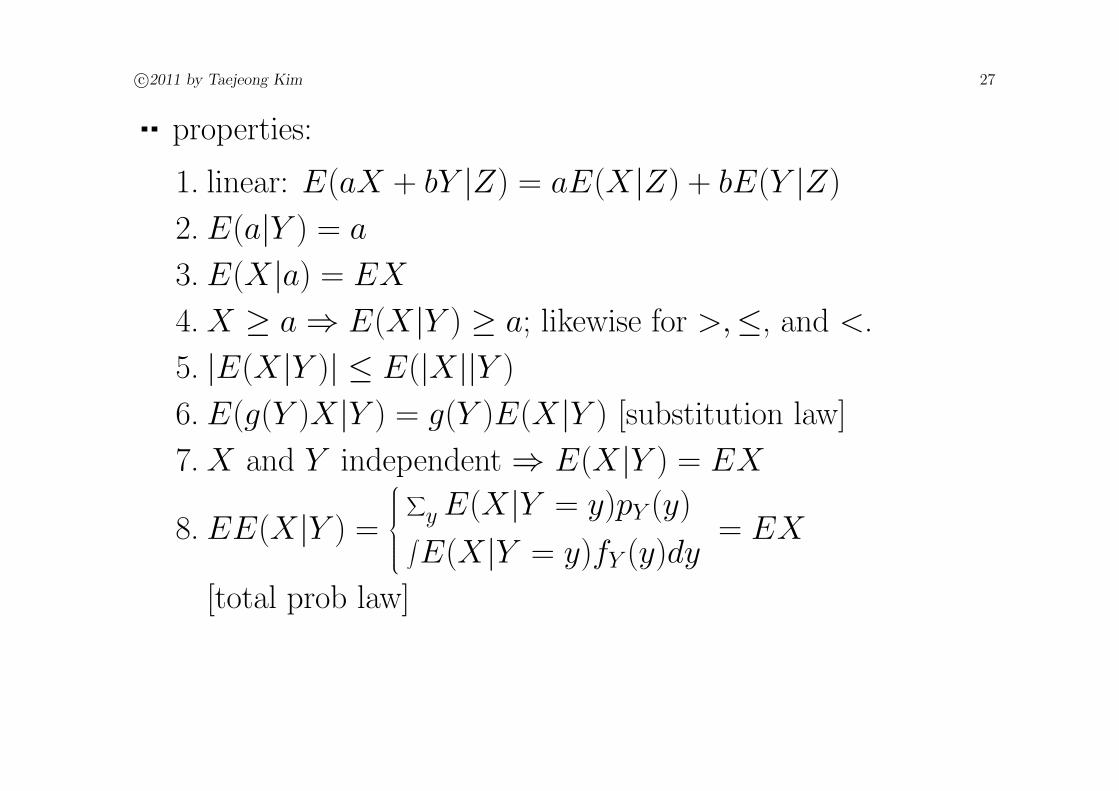
properties:
1. linear: E(aX + bY |Z) = aE(X|Z) + bE(Y |Z)
2. E(a|Y ) = a
3. E(X|a) = EX
4. X ≥ a ⇒ E(X|Y ) ≥ a; likewise for >,≤, and <.
5. |E(X|Y )| ≤ E(|X||Y )
6. E(g(Y )X|Y ) = g(Y )E(X|Y ) [substitution law]
7. X and Y independent ⇒ E(X|Y ) = EX
8. EE(X|Y ) =
∑y E(X|Y = y)pY (y)
∫E(X|Y = y)fY (y)dy
= EX
[total prob law]

c©2011 by Taejeong Kim 28
y1
y2
y3
y4
X
E(X|A1)
E(X|A2)
E(X|A3)
E(X|A4)
A1 A2 A3 A4
Y
U
V
Assume that the probability is uniformly allocated over Ω.

c©2011 by Taejeong Kim 29
9. E[E(X|Y )|g(Y )] = E[X|g(Y )]
E[E(X|C)|B] = E(X|B),
where B and C are σ-fields such that B(coarser) ⊆ C(finer).g(Y ) generates a smaller σ-field than Y does.
E[E(X|Y )|a] = E(X|a) = EX , which corresponds to
E[E(X|C)|B] = E(X|B), where B = ∅, Ω.10. E[E(X|g(Y ))|Y ] = E[X|g(Y )] [function of Y ]
E[E(X|B)|C] = E(X|B),
where B and C are σ-fields such that B ⊆ C.
11. g is one-to-one ⇒ E[X|g(Y )] = E(X|Y )
Y and g(Y ) generate the same σ-field.

c©2011 by Taejeong Kim 30
12. E(X|Y ) is the optimal mmse (minimum mean square error)estimator of X given Y . That is, among all functions of Y ,g(Y ) = E(X|Y ) minimizes the mean square error given by
E[X − g(Y )]2.
We will discuss later in detail linear and nonlinear mmseestimators for random vectors, of which random variablesare special cases.

c©2011 by Taejeong Kim 31
Cumulative distribution function
• cumulative distribution function, cdf
FX(x) := P (X ≤ x)
For discrete X , FX(x) consists of discrete steps.The step heights are the probability masses.
FX(x) =∑
v≤x pX(v) =∑
v pX(v)u(x−v), u(x) :=
1, x ≥ 00, x < 0
example: Ber(p) cdf
-
6
v
v
0 1
1−p1
For continuous X , FX(x) is absolutely continuous and dif-ferentiable (almost everywhere: a.e.).
FX(x) =∫ x−∞ fX(v)dv; fX(x) = dFX(x)/dx

c©2011 by Taejeong Kim 32
absolutely continuous F (x): ∀ ε > 0,∃ δ > 0 such that
for every pairwise disjoint (ai, bi), i = 1, ···, k,∑k
i=1 (bk − ak) < δ ⇒ ∑ki=1 |F (bk)− F (ak)| < ε
F is absolutely continuous and differentiable a.e. with thederivative f . ⇔ f is integrable and F (x) = F (a)+
∫ xa f (v)dv.
example: The Cantor function is continuous but not ab-solutely continuous.
- - -

c©2011 by Taejeong Kim 33
example: cdfs, unif(a,b) and N(m,σ2)
-
6
´´
´´
´´
´´
a b
1
-
6
m
1
properties:
1. 0 ≤ FX(x) ≤ 1
2. P (a < X ≤ b) = FX(b)− FX(a)
3. limx→−∞FX(x) = 0
4. limx→∞FX(x) = 1
5. monotone non-decreasing
6. right continuous: limε→0 FX(x + ε) = FX(x)
7. limε→0 FX(x− ε) = FX(x)− P (X = x)

c©2011 by Taejeong Kim 34
Gaussian cdf : Φ(x) := 1√2π
∫ x−∞ e−u2/2du
X ∼ N(m,σ2): FX(x) = Φ((x−m)/σ)
Q function: Q(x) := 1− Φ(x), complementary to cdf
error function: erf(x) := 2√π
∫ x0 e−u2
du
complementary error function:
erfc(x) := 1− erf(x) = 2√π
∫ ∞x e−u2
du
erfc(x) = 2Q(√
2x), Q(y) = 12erfc
y√2
Detection error probabilityX = s + N
under additive Gaussiannoise is expressed by thesefunctions.

c©2011 by Taejeong Kim 35
random number generation
One can obtain a random variable Y that has the target cdfF (y) by transforming X ∼ unif(0,1) through a function g suchthat Y = g(X).
-
6
¡¡
¡¡
¡¡
FX(x)
1 xpppppppppp
p p p p p p p p p p1
We want FY (y) = P (Y ≤ y) = F (y).
For monotone increasing invertible g(x),
FY (y) = P (g(X) ≤ y) = P (X ≤ g−1(y)) = FX(g−1(y)).
FX(x) = x for x ∈ [0, 1] ⇒ FY (y) = g−1(y) = F (y)
⇒ g(x) = F−1(x) if invertible
Therefore, if g(x) = F−1(x), then FY (y) = F (y).
Note that we only need to define g(x) for x ∈ [0, 1].

c©2011 by Taejeong Kim 36
example: X ∼ unif(0,1), F (y) =
0, y < 01− e−y, y ≥ 0
Let g(x) = F−1(x) = − ln(1− x) for x ∈ [0, 1].
Then we have FY (y) = F (y), ie, Y ∼ exp(1).
-
6
1
F (y) = FY (y)
y-
6
1
g(x)
x
If F−1(x) does not exist, as in the case of a discrete randomvariable, we can use a “pseudo-inverse”.

c©2011 by Taejeong Kim 37
example: X ∼ unif(0,1), Y ∼ bin(3,1/3)
FY (y) =
0, y < 08/27, 0 ≤ y < 120/27, 1 ≤ y < 226/27, 2 ≤ y < 31, y ≥ 3
, g(x) =
0, 0 ≤ x ≤ 8/271, 8/27 < x ≤ 20/272, 20/27 < x ≤ 26/273, 26/27 < x ≤ 1
-
6
0 1 2 3
827
2027
2627 1FY (y)
-
6
0 827
2027
2627
1
1
2
3
g(x)

c©2011 by Taejeong Kim 38
Central limit theorem
X1, X2, · · · are iid with mean m and variance σ2.
Sn =∑n
i=1 Xi: mean=nm, var=nσ2
Mn = 1n
∑ni=1 Xi: mean=m, var=σ2/n
Zn = 1√n
∑ni=1 Xi: mean=
√nm, var=σ2
Yn = 1√n
∑ni=1
Xi−m
σ
: mean=0, var=1
u
uXi
n=2
n=5
n=10
uu
u
Sn
uu u
u u u
u u u u u u u u u u u
uu
u
Mn
uuuuuu
uuuuuuuuuuu
uu
u
Zn
uuu
uuu
uuuuuuuuuuu

c©2011 by Taejeong Kim 39
0 5 10 15 20 25
0.129 -
bin(50, 1/4):
50k
14
k
34
50−k
Mn = 1n
∑ni=1 Xi, Xi∼unif

c©2011 by Taejeong Kim 40
central limit theorem: limn→∞FYn(y) = Φ(y).
Or equivalently, limn→∞ϕYn(u) = exp(−u2/2).
proof: ϕYn(u) = EejuYn = E expju
∑i Wi√n
, where Wi = Xi−m
σ
=∏
i E expjuWi√
n
=
E exp
juW√
n
n
[iid: Wi]
ln ϕYn(u) = n lnE exp
juW√
n
= n lnE
1 + juW√
n− u2W 2
2n− ju3W 3
3!n3/2 + u4W 4
4!n2 − · · ·
= n ln1− u2
2n− Rn
n
, where limn→∞Rn = 0
= n ln1− 1
n
u2
2+ Rn

c©2011 by Taejeong Kim 41
Since ln(1− x) = −x + x2
2+ x3
3+ · · ·
for |x| < 1,
ln ϕYn(u) = n ln1− 1
n
u2
2+ Rn
= −n1n
u2
2+ Rn
+ 1
2n2
u2
2+ Rn
2+ 1
3n3
u2
2+ Rn
3+ · · ·
= −
u2
2+ Rn
+ 1
2n
u2
2+ Rn
2+ 1
3n2
u2
2+ Rn
3+ · · ·
→ − u2
2as n →∞.
This convergence is quite fast, so as few as 6 or 12 iid uniformrandom variables are often added to approximate a Gaussianrandom variable.
This type of convergence,Yn converging to N(0,1), is calledconvergence in distribution.

c©2011 by Taejeong Kim 42
Mixed random variable
When the cdf of a random variable is piecewise continuous withjumps, we can use neither pmf nor pdf to describe its distribu-tion.⇒ We need to generalize pmfs and pdfs into generalized pdfs.
Dirac delta function:
δ(x) := limε→0 dε(x), where dε(x) =
1/ε, −ε/2 ≤ x ≤ ε/20, else
∫ ∞−∞ δ(x)dx =
∫ ε−ε δ(x)dx =
∫ u+εu−ε δ(x− u)dx = 1
- - -¾-
ε
?
6
1/εg(x)
u ¾-
εε
?
6
1

c©2011 by Taejeong Kim 43
sifting property: For g(x) continuous at u,∫ ∞−∞ g(x)δ(x− u)dx = limε→0
∫ ∞−∞ g(x)dε(x− u)dx
= limε→01ε
∫ u+ε/2u−ε/2 g(x)dx = g(u).
unit step function: u(x) =
1, x ≥ 00, x < 0
u(x) =∫ x−∞ δ(v)dv, δ(x) = du(x)
dx
For a discrete random variable X ,
FX(x) =∑
i pX(xi)u(x− xi)
fX(x) = dFX(x)dx
=∑
i pX(xi)δ(x− xi): generalized pdf
EX =∫xfX(x)dx =
∫x(
∑i pX(xi)δ(x− xi))dx
=∑
i pX(xi)∫xδ(x− xi)dx =
∑i xipX(xi)

c©2011 by Taejeong Kim 44
This shows the generalized pdf works in computing expecta-tion.
example: Consider tossing a coin; if a head turns up, pick a realnumber randomly from [0,4]; if a tail, pick a number among1, 2, 3. The resulting number is a mixed random variable X .The (generalized) pdf:
fX(x) = fX|H(x)P (H) + fX|T (x)P (T ) [total prob law]
=
14· 1
2+
∑3
i=113δ(x− i)
· 1
2, 0 ≤ x ≤ 4
0, else
=
18
+ 16
∑3i=1 δ(x− i), 0 ≤ x ≤ 4
0, else

c©2011 by Taejeong Kim 45
-
6
6 6 6
1 2 3 4 x
18
fX(x)
-
6
³³³
³³³
³³³
³³³
1 2 3 4 x
FX(x)
For a mixed random variable, there is α ∈ (0, 1) such that
FX(x) = αFc(x) + (1− α)Fd(x),
where Fc(x) is continuous, and Fd(x) consists of steps.
fX(x) = αfc(x) + (1− α)fd(x),
where fc(x) is a regular, non-generalized pdf, and fd(x) consistsof delta functions.

c©2011 by Taejeong Kim 46
Joint cdf
• joint cumulative distribution function, jcdf
FXY (x, y) := P (X ≤ x, Y ≤ y)
-
6
q q q q q q q q q q q q q q q q q q q qq q q q q q q q q q q q q q q q q q q qq q q q q q q q q q q q q q q q q q q qq q q q q q q q q q q q q q q q q q q qq q q q q q q q q q q q q q q q q q q qq q q q q q q q q q q q q q q q q q q qq q q q q q q q q q q q q q q q q q q qq q q q q q q q q q q q q q q q q q q qq q q q q q q q q q q q q q q q q q q qq q q q q q q q q q q q q q q q q q q qq q q q q q q q q q q q q q q q q q q qq q q q q q q q q q q q q q q q q q q q(x,y)
X
Y
-
6
q q q q q q q q qq q q q q q q q qq q q q q q q q qq q q q q q q q qq q q q q q q q q(a,d) (b,d)
(a,c) (b,c)
X
Y
properties:
1. 0 ≤ FXY (x, y) ≤ 1
2. P (a < X ≤ b, c < Y ≤ d)
= FXY (b, d)− FXY (a, d)− FXY (b, c) + FXY (a, c)

c©2011 by Taejeong Kim 47
3. limx→−∞FXY (x, y) = 0; limy→−∞FXY (x, y) = 0
4. limy→∞FXY (x, y) = FX(x): marginal cdf
limx→∞FXY (x, y) = FY (y): marginal cdf
5. limx→∞,y→∞FXY (x, y) = 1
6. monotone non-decreasing in x and y
7. right continuous in x and y:
limε→0 FXY (x + ε, y) = FXY (x, y)
limε→0 FXY (x, y + ε) = FXY (x, y)
8. limε→0 FXY (x− ε, y) = FXY (x, y)− P (X = x, Y ≤ y)
limε→0 FXY (x, y − ε) = FXY (x, y)− P (X ≤ x, Y = y)
9. independent X and Y ⇔ FXY (x, y) = FX(x)FY (y)

c©2011 by Taejeong Kim 48
For jointly discrete X and Y , FXY (x, y) consists of discrete 2-dsteps, each looking like a corner of a box. The step heights arethe probability masses, but not always.
FXY (x, y) =∑∑
v≤x,w≤y pXY (v, w)
=∑∑
v,w pXY (v, w)u(x− v)u(y − w)
example:
-
x¡¡
¡¡
¡¡
¡¡
¡¡
¡¡µypXY (x, y)
u
u
uu
¡¡
¡¡¡
¡¡
¡¡¡
¡¡
¡¡¡
-¡
¡¡
¡¡
¡
FXY (x, y)
x
¡¡
¡¡
¡¡
¡¡
¡¡
¡
¡¡
¡¡
¡¡¡
¡¡
¡¡
¡¡

c©2011 by Taejeong Kim 49
-
x¡¡
¡¡
¡¡
¡¡
¡¡
¡¡µzpXZ(x, z)
u u
u u
¡¡
¡
¡¡
¡
¡¡
¡
-
x¡¡¡
¡¡µz
FXZ(x, z)
¡¡
¡¡
¡¡
¡¡
¡
¡¡
¡
¡¡
¡¡¡
¡¡
¡

c©2011 by Taejeong Kim 50
For jointly continuous X and Y , FXY (x, y) is absolutely con-tinuous in each variable.
fXY (x, y) = lim∆x→0,∆y→0P (x<X≤∆x, y<Y≤∆y)
∆x∆y
= lim FXY (x+∆x,y+∆y)−FXY (x+∆x,y)−FXY (x,y+∆y)+FXY (x,y)∆x∆y
= ∂2FXY (x,y)∂x∂y
= lim|∆|→0P [(X,Y )∈∆]
|∆|FXY (x, y) =
∫ x−∞
∫ y−∞ fXY (v, w)dvdw

c©2011 by Taejeong Kim 51
Jointly Gaussian random variables
jpdf:
fXY (x, y) =1
2πσXσY
√
1− ρ2exp
−x2 − 2ρxy + y2
2(1− ρ2)
,
where x = (x−mX)/σX and y = (y −mY )/σY .
⇒ Jointly Gaussian random variables are fully characterizedby their 1-st and 2-nd moments, ie, their means, variances, andcovariance.
x
y
ρ = 0
-
6
x
y
ρ > 0
-
6
contour lines

c©2011 by Taejeong Kim 52
marginal pdfs:
fX(x) = 1√2πσX
exp
−(x−mX)2
2σ2X
= 1√
2πσXexp
−x2
2
fY (y) = 1√2πσY
exp
−(y−mY )2
2σ2Y
= 1√
2πσYexp
−y2
2
cpdf:
fX|Y (x|y) =1√
2πσX|yexp
−(x−mX|y)2
2σ2X|y
,
where
mX|y = mX + ρσXσY
(y −mY ) is the conditional mean and
σ2X|y = σ2
X(1− ρ2) is the conditional variance.
⇒ σ2X|y ≤ σ2
X

c©2011 by Taejeong Kim 53
⇒ E(X|Y = y) = mX|y = mX + ρσXσY
(y −mY )
⇒ E(X|Y ) = mX + ρσXσY
(Y −mY )
Note that this is an affine function of Y , while the conditionalexpectation is generally nonlinear function of Y .
If ρ = 0, ie, uncorrelated, then mX|y = mX and σ2X|y = σ2
X.
⇒ fX|Y (x|y) = fX(x)
⇒ X and Y are independent.
Thus, if jointly Gaussian random variables are uncorrelated,they are independent. This is not true in general.

c©2011 by Taejeong Kim 54
jchf: ϕXY (u, v)
= exp
j(mXu + mY v)− 1
2(σ2
Xu2 + 2ρσXσY uv + σ2Y v2)
It is easy to see in this (also in the jpdf) that uncorrelatednessimplies independence.
X and Y are jointly Gaussian.
⇒ aX + bY and cX + dY are jointly Gaussian.
X and Y are iid Gaussian with mean zero.
⇒ U =√
X2 + Y 2 is Rayleigh,
V = 6 (X,Y ) is uniform,
and U and V are independent.
⇒ fXY (x, y) is isotropic.

c©2011 by Taejeong Kim 55
X and Y are iid Gaussian with mean zero and variance 1.
⇒ U 2 = X2 + Y 2 is chi-squared with 2 degrees of freedom,
which is exp(1/2).
Xi are iid Gaussian with mean zero and variance 1.
⇒ ∑ki=1 X2
i is chi-squared with k degrees of freedom.
independent Gaussian X and Y
⇒ X/Y is Cauchy.