rp0284 – climate-induced international migration and · rp0284 – climate-induced international...

RP0284 – Climate-induced international migration and conflicts

Research Papers Issue RP0284 January 2017

By Cristina Cattaneo Fondazione Eni Enrico

Mattei (FEEM) and Fondazione Centro Euro-

Mediterraneo sui Cambiamenti Climatici

(CMCC) [email protected]

SUMMARY Population movements will help people cope with the impacts of climate change. However, large scale displacements may also produce security risks for receiving areas. If climate change intensifies the process of out-migration, destination countries may face waves of migrants so large and fast that integration becomes increasingly hard. The objective of this paper is to empirically estimate if the inflows of climate-induced migrants increase the risk of conflicts in receiving areas. Using data from 1960 to 2000, we show that climate-induced migrants are not an additional determinant of civil conflicts and civil wars in receiving areas.

Valentina Bosetti Department of Economics,

Università Bocconi, Fondazione Eni Enrico

Mattei (FEEM) and Fondazione Centro

Euro-Mediterraneo sui Cambiamenti Climatici

(CMCC) [email protected]

Keywords Conflict, Global Warming, Emigration

TheresearchleadingtotheseresultshasreceivedfundingfromtheItalianMinistryofEducation,

UniversityandResearchandtheItalianMinistryof

Environment,LandandSeaundertheGEMINA

project.

ECIP – Economic analysis of Climate Impacts and Policy

Division

JEL Codes Q54, F22, Q34, H56

2

1. Introduction

In the coming decades, climate change will expose hundreds of millions of people to its impacts. As

summarized by the main scientific intergovernmental body on climate change in its latest report (IPCC,

2014), both vulnerability and exposure will be extremely diverse across the globe. The migration of

individuals and communities from the areas most exposed to environmental stress represents and will

represent an important measure of adaptation to climate change. However, the resulting displacements may

also produce security risks for receiving areas.

The direct link between climate change and emigration, on the one hand, and between climate

change and violent conflicts, on the other, have been both researched individually. For example, Barrios et

al. (2006) find that rain shortages increase internal migration from rural to urban areas in Sub-Saharan

countries. Marchiori et al.(2011) report that temperature and rainfall anomalies affect both internal and

international migration in sub-Saharan countries. They also predict that weather anomalies will produce an

annual displacement of more than 11 million people by the end of the 21st century. Cai et al. (2016) report a

positive effect of yearly temperatures on bilateral migration flows directed to OECD countries from both

middle and low income countries, while Cattaneo and Peri (2016) find that the positive effect of rising

temperature on emigration rates to urban areas and to other countries features only in middle income

economies. In very poor countries, higher temperatures reduce the probability of emigration to cities or to

other countries, consistently with the presence of liquidity constraints. Conversely, Beine and Parsons (2015)

find no statistical significant effect of climate-related factors such as extreme weather events, deviations and

anomalies from the long-run averages, on bilateral international migration. The null effect features in all

origin countries, independently of the level of income.

Regarding the second nexus, namely between climate and violent conflicts, Miguel et al. (2004) is

the first paper that includes rainfall-driven economic shocks in a conflict estimation for sub-Saharan

countries. They find that lower rainfall levels and adverse rainfall shocks increase the likelihood of conflicts

in African countries. Further evidence of a possible link comes from Hsiang et al. (2011) documenting more

likely conflicts during hot and dry El Nino years than during cooler La Nina years. Harari and La Ferrara

(2014) also report that climatic shocks increase conflicts in a geographically disaggregated analysis.

Conducting a meta-analysis on quantitative studies Hsiang et al. (2013) conclude that warming is associated

3

with an increase in both the rate of interpersonal conflict and the rate of intergroup conflict. Burke et al.

(2009) find a strong link between civil war and temperature in Africa, if one controls for country fixed

effects and country-specific time trends only.

However, it appears that the results are not robust to different statistical assumptions and different

specifications in the corresponding papers. For example, Ciccone (2011) reconsiders the link between

rainfall and conflict found in Miguel et al. (2004). By taking into account the mean-reverting properties in

rainfall, the author finds no robust link between civil conflicts and year-on-year rainfall growth or rainfall

levels. Couttenier and Soubeyran (2014) document that any statistically significant relationship between

climate variables and conflict vanishes if one takes into account yearly worldwide changes in civil war and

the evolution of rainfall and temperature. When year fixed effects are included, the coefficient of the climatic

variables drastically reduces and turns not significant compared with a specification with no year fixed

effects. Buhaug (2010) finds that in African countries climate variability is poorly related to armed conflict.

The paper improves with respect to the previous literature by considering not only civil wars, which are

battleswithat least 1,000 deaths but also conflicts with a lower number of deaths, setting the threshold to 25

annual battle deaths. In addition, the author models the outbreak and incidence of civil war as distinct

processes. To summarize, results seem to be highly sensitive to the way climate is modelled, to changes in

the data and in the coding choices and to the use of yearly fixed effects that should take into account

coincident movements in the aggregate measures of climate and civil conflict.

The possibility that climate, migration and conflict are interlinked has been envisaged and discussed,

in some of these studies, but only qualitatively. The causal link has not been adequately tested (Withagen,

2014). Indeed, some of the above studies find that natural disasters increase the risk of conflicts, but don't

explore the specific channels through which this relationship emerges. A sudden and mass influx of

displaced people can be one of these channels, in particular when poor economic conditions and weak

institutions characterize the receiving regions. Extreme climatic events such as floods, droughts, extreme

heat may intensify the process of out-migration to a point that large and fast waves of migrants are not

smoothly absorbed in destination countries, and this can ultimately make conflicts more likely. This threat

could be exacerbated by competition over resources, ethnic tensions, distrust, demolition of social capital and

crossing of fault lines (Reuveny, 2007). The threat could also arise if climatic shocks in hosting countries are

4

correlated with shocks in sending locations. However, we should expect that people move from areas most

exposed to climate shocks to less climate-vulnerable areas.

Ghimire et al. (2015) is the only paper that analyses the link between climate-related human

displacement and civil conflict. The paper uses historical data for 126 countries during 1985–2009 and finds

that the displacement of people due to floods is not a cause of new conflicts. However they find that

migration induced by floods contributes to prolong existing conflicts. The paper focuses only on flood-

induced displacement. It is well known, however, that other events, such as gradual changes in temperature,

droughts, changing patterns of precipitations or heat waves can influence migration (IPCC, 2014) and this

can consequently generate conflicts (Hsiang et al., 2013). The number of displaced people and the risk of

conflict could then be different from the figures reported in Ghimire et al. (2015), if one were to consider a

broader definition of climate change as a driver of migration. Moreover, the paper considers only internally

displaced people, namely people who move within the same country. It does not consider the effect of

international migration on conflict in destination countries. This is an important distinction between the

present paper and the one by Ghimire at al. (2015).

The objective of the paper is to analyse whether gradual changes in temperature and precipitations or

the occurrence of extreme events such as flood, droughts and storms have an impact on conflicts through the

migration channel. To answer this question a macro level empirical estimation is conducted. The rest of the

paper is organized as follows. Section 2 describes the methodology to compute the measure of climate-

migrants. Section 3 presents a description of the data and the empirical specifications. Section 4 shows the

results. Section 5 provides a summary and conclusions.

2. Methodology to compute a measure for climate-migrants

This paper addresses the nexus between migration, conflict and climate change applying a multiple-step

approach. The aim is to estimate the indirect impacts of environmental stress on conflicts through migration.

However, in order to test the relationship between the flows of environmental migrants towards destinations j

on conflicts in country j, we need a measure for climate-induced inflows. This data is not available as such.

Census and other migration datasets do not include information on the reasons for migration. It is extremely

difficult to identify migrants that have left their homelands solely due to environmental stressors. To

5

overcome this constraint, we follow the approach developed in Peri (2005), in the context of knowledge

spillovers.1 Similarly, we build the number of climate-migrants by predicting the total emigration flows

departing from country c due to climate change. In particular, we estimate the following equation:

𝐸𝑀#,% = 𝛼) + 𝛽)𝑇#,% + 𝛾)𝑃#,% + 𝛿)𝐹#,% + 𝜃)𝐷#,% + 𝜅)𝑆#,% + 𝜙6,% + 𝜀#,% i=L, M, H (1)

where 𝐸𝑀#,% is net emigration flows from origin country c in decade beginning with year t (= 1960, 1970,

1980, 1990). Climate change will be expressed not only through gradual changes in temperature and

precipitation, but we can expect that extreme conditions such as droughts, floods and storms will

increasingly become the norm. Eq. (1) represents a reduced-form relationship between climate realization

and emigration and reflects the variation in emigration flows driven by temperature, precipitation and

extreme events. Variations in the predicted values of 𝐸𝑀#,% will be driven solely by the country's climatic

characteristics and not by other country-specific factors that are independent of the climate.

Drawing on Cattaneo and Peri (2016), we estimate equation (1) allowing for differential effects on

emigration between low, middle and high income countries. All coefficients are estimated for three groups of

countries, namely low (L), middle (M) and high income (H) countries, using the World Bank income

classification (World Bank, 2016).

T and P are average temperature and precipitation in country c, over the decade t. F, D and S are the

number of floods, droughts and storms that occurred during the decade t.2 𝜙6,%captures region-decade

dummies in order to absorb regional factors of variation in economic conditions over time, thus alleviating

potential omitted variable bias. Finally 𝜀#,%is a random error term, clustered by country of origin.

Following Jones and Olken (2010), Dell. et al. (2012), Couttenier and Soubeyran (2014), Hsiang et

al. (2013) and Cattaneo and Peri (2016) no additional controls are added to Eq. (1). Climatic variables affect

many of the socioeconomic factors commonly included as control variables. Things like income, population, 1Peri (2005) needs to generate the share of the knowledge flowing from one country to another given that these data are not available. He predicts this share by using an auxiliary regression.2 The choice to build a variable that counts the number of floods, droughts and storms that occurred during the decade, rather than a measure of the intensity of the events, measured as the total number of deaths or total damage, is two-fold. First we want to minimize the measurement error of the variable, which may occur if one uses the total number of deaths or total economic damage. Second, all variables have to be computed as 10 years average. The number of deaths or total economic damage have strong variation along the 10-year interval. The use of the average of the total damage would under-estimate the effect of the disaster.

6

socio-political environment are themselves an outcome of climate. If these outcome variables are used as

controls, we may draw mistaken conclusions about the relationship between climate and migration. The

inclusion of these additional controls in addition to temperature, precipitations, droughts, floods and storms

would produce a bad control problem, also called over-controlling problem (Dell. et al., 2012).

The estimation of Eq. (1) applying decadal data allows one to capture medium-run impacts of

climate change. Changes of temperature, precipitations or incidence of extreme events over annual periods

have a distinct effect from the medium-run changes. Adaptation is one crucial mechanism that drives a

wedge between short-run and medium-run impacts. The advantage of taking decadal data is that one can

partially embody the adaptation effects and can better identify medium-run effects.

Using the estimated parameters of temperature and precipitation from Eq. (1) we build a predicted

measure of the climate-induced emigration flows for every country in the sample. In a following step, we

allocate the emigration flows departing from country c due to climate change to the different possible

destinations j. To do so, we use the observed shares of total emigration flows from country c to country j , at

time t, 𝑆#8,%.

The assumption that climate-induced migrants are distributed across the different destinations as all

other migrants follows from the strong empirical evidence that migration networks play an important role in

the choice of the destination. By summing over all the countries of origin we can compute climate-migrants

in all destinations j.

𝐼𝑀8,% = 𝑆#8,% ∗ 𝐸𝑀#,%# (2)

Once the inflows of climate-induced migrants are predicted for each destination j, we include this variable in

a conflict equation.

3. Data and Empirical Specification

The migration data are taken from Ozden et al. (2011), which give bilateral migration stocks between 226

origin and destination countries for the last five censuses rounds, 1960-2000. The data are only available

every ten years. We compute net emigration flows as differences between stocks of foreigners in two

7

consecutive Censuses. Temperature and precipitation data are taken from Dell et al. (2012). The authors

aggregate worldwide (terrestrial) monthly mean temperature and precipitation data at 0.5 X 0.5 degree

resolution obtained from weather stations (Matsuura and Willmott, 2007)3 using as weights 1990 population

at 30 arc second resolution from the Global Rural-Urban Mapping Project (Balk et al. 2004). The country

level data for floods, storms and droughts are taken from EM-DAT, an International Disaster Database

compiled by the Centre for Research on the Epidemiology of Disasters (Guha-Sapir et al., 2015). Applying a

simple two-period model in the spirit of Roy-Borjas (Roy, 1951; Borjas, 1987), Cattaneo and Peri (2016)

provide theoretical predictions of the effect of temperature and emigration, which vary depending on the

income of the origin country. In particular, the authors predict that an increase in average temperature

increases emigration rates in middle-income countries, decreases emigration rates in poor countries, and

should not affect emigration in rich countries.

As far as conflict is concerned, we take the data from the UCDP/PRIO Armed Conflict Dataset,

which is the most widely used source of conflict data at the country level. The dataset offers a yearly binary

indicator of the existence of a conflict in a specific country, based on the number of deaths per year. This

variable focuses only on civil conflicts, which are coded under the categories 3 and 4 of the PRIO database.4

We use data over the period 1960-2000. The following decade specification is estimated:

𝐶8,% = 𝛼 + 𝛽𝐼𝑀8,% + 𝜑 ln 𝐺𝐷𝑃8,% + 𝛾 ln 𝑃8,% + 𝛿𝐷8,% + 𝜓𝑂8,% + 𝜃𝑁8,% + 𝑰𝒋,𝒕F 𝜆 + 𝜋𝐺8,% + 𝜁𝑀8,% +

𝜙% + 𝜀8,% (3)

𝐶8,% is a dummy variable, equal to one if at least one civil conflict occurred in the decade beginning with year

t (=1960, 1970,1980,1990) in the country j, and zero otherwise. Country j is the destination country of the

specific flows of climate-migrants. This variable captures the incidence of a civil conflict. Alternatively, it is

3Terrestrial Air Temperature and Precipitation: 1900--2006 Gridded Monthly Time Series, Version 1.014 UCDP/PRIO Armed Conflict Dataset distinguishes between four types of conflict. Civil conflicts are categorized as “Internal armed conflict occurs between the government of a state and one or more internal opposition group(s) without intervention from other states” and as “Internationalized internal armed conflict occurs between the government of a state and one or more internal opposition group(s) with intervention from other states (secondary parties) on one or both sides”.

8

equal to one if at least one civil conflict started in the decade t in country j.5 In this case the variable

measures the onset of a civil conflict. The onset specification answers to the question of what makes a

"fresh" episode of violence break out, while the incidence specification captures the total intensity of a

conflict. In our baseline specification, civil conflicts refer to battles with at least 25 deaths in a given year. In

a robustness check we will use the alternative threshold based on 1000 or more deaths per year. In this case,

the dependent variable measures civil wars. 𝐼𝑀 is the climate-induced net immigration flows, predicted from

Eq. (2).

Given that a dichotomous variable fails to utilize a lot of information on conflict, in an alternative

specification we use a count variable for the number of conflicts. Finally, following Cotet and Tsui (2013)

we also measure conflicts by the military coup attempts, from the Center for Systemic Peace (CSP). 𝐼𝑀 is

the inflows of climate-induced migrants calculated as in Eq. (2).

We use a standard battery of controls, which have been previously applied in the conflict literature

(among others Fearon and Latin, 2003; Montalvo and Reynal-Querol, 2005; Montalvo and Reynal-Querol,

2008; Esteban et al., 2012; Esteban et al., 2015; Morelli and Rohner, 2015). Fearon and Latin (2003) provide

a detailed description of the rationale for the inclusion of the full set of controls. We include the natural

logarithm of GDP per capita and the natural logarithm of population (P). We add an index of ethnic

fractionalization (D), natural resource abundance (O) which identifies countries where fuel exports exceed

one third of merchandise exports, and a control for whether a state was recently created (N), marking

countries in the first ten years of independence. We include a vector of controls for institutional quality (I),

using the Polity-2 score from the Polity IV database. To allow for a non-linear effect of institutional quality,

we decompose this index to capture democracies, which are countries with an index higher than six,

anocracies between minus five and plus five and autocracies lower than minus six. We add a control for non-

contiguous states (G) and for mountainous terrain (M), which measures the percentage of territory covered

by mountains. 𝜙% is a decade fixed effect. All controls are averaged over a time period of ten years of the

decade t. In an alternative specification, we measure the controls in the year starting decade t.6 Table A1 in

5 To compute the onset variable, we first computed the onset variable on a yearly basis. The yearly onset variable is equal to one in the starting year of the conflict and zero in the following years unless a new conflict started. The decade onset variable then measures if a conflict initiated in decade t. 6 Montalvo and Reynal-Querol (2005) and Esteban et al. (2012) estimate a similar sub-period specification using 5-year intervals. In these papers, controls are measured in the first year of each period.

9

the Appendix provides a summary statistics of the variables, while Appendix C provides information of the

different sources of the variables.

We use linear probabilities models in the estimations as they have been extensively used in the

literature (Berman et al. 2017; Cattaneo et al., 2014). They allow a straightforward computation of the

marginal effects and are a convenient approximation to the underlying response probability (Wooldridge,

2010).

As most of the existing empirical literature, we run pooled cross-country regressions without

controlling for country fixed effects (see for example, Fearon and Laitin, 2003; Montalvo and Reynal-

Querol, 2005; Montalvo and Reynol-Querol, 2008; Esteban et al. 2012; Esteban et al. 2015). We do so for

two main reasons. First, averaging all variables over ten years, we remove a big part of the within country

variation in the controls. The inclusion of country fixed effects would likely remove the significance of most

control variables in this context. Second, an important determinant of civil conflicts, such as ethnic

fractionalization, is not a time-varying measure. Given that the inflows of migrants may alter the ethnic

composition of the destination countries, the inclusion of the ethnic diversity is crucial. The effect of ethnic

diversity would be absorbed by the migration variable, if one does not include this control in the regression.

To address concerns of unobserved heterogeneity between countries leading to over-stated significance

levels, we cluster standard errors by country. We also estimate different sets of specifications, which include

regional fixed effects, or alternatively region-decade fixed effects. This is done following Esteban et al.

(2015), Montalvo and Reynal-Querol (2008).

An additional concern is represented by the fact that our control of interest, climate-induced

migration (𝐼𝑀) is a generated regressor (Pagan, 1984). Inference in case of generated regressors is

problematic as the sampling variation of the vector of parameters of the first step estimation is unknown. To

address this problem we employ bootstrapped standard errors.

4. Results

Table 1 provides the estimated coefficients of Eq. (1). Column (1) displays results of a specification which

includes interaction between decade and region fixed effects to control for regional factors of variation in

economic conditions over time. Column (2) adds also decade fixed effects interacted with a high income

10

country dummy, to capture differential time variation in the group of countries considered as “high income”

relative to those considered as “middle” or “low” income. Rich countries should behave differently

compared to other groups as agriculture represents only a small source of income and the rural population is

a small percentage of the total compared to middle and low income countries.

The point estimates are quite stable across specifications. Moreover, they indicate differential

impacts of climate change depending on the income level of the origin countries.7 Migration from middle

income countries is positively driven by the incidence of floods and storms and decreases with higher

precipitation. On the contrary, the coefficient of average temperature is not statistically significant at the

conventional levels. These findings indicate that in middle income countries, fast-onset rather than slow-

onset events encourage emigration. The existing literature agrees on the fact that migration responses to

slow-onset environmental change differ from those to rapid-onset events. For example, by analysing four

different articles, Fussell et al. (2014) conclude that rapid onset weather events produce evacuation or

displacement of entire households. This type of migration can occur over a longer period of time even if

return episodes are sometimes documented. On the contrary, slow-onset events tend to produce short

distance and temporary migration. This is a type of migration that the present analysis does not capture,

given that migration data arte taken from Censuses. An additional flooding event in middle income countries

increases the net emigration flows by 16’564 persons. As the average emigration flows from middle income

countries are 234’910, an additional flood would increase the emigration flows by about seven percent.

Conversely, extreme events do not produce an increase in migration from low income countries.

Even if we would expect to see migration in response to extreme events, such as a floods, from poor

countries as well, as floods destroy homes and farms, it could be that this type of climatic shock is so

detrimental that it traps very poor people and makes them unable to migrate. Floods worsen the liquidity

constraint of people who live near subsistence in poor countries, , implying a reduced ability to pay for

migration costs. Environmental change on the one hand increases the incentive to move, but on the other it

can also limit the capacity to do so (Black et al., 2011). Climate change can reduce mobility through resource

constraints (Fussell et al., 2014). An increase in precipitation, on the contrary, reduces emigration from low

income countries. In many countries, where farmers barely have access to irrigation, precipitation represents 7F-testsontheequalityofcoefficientsforthedifferentgroupsofcountriesareconductedandconfirmthedifferentresponsewithrespecttoflood,drought,stormandprecipitation.

11

an environmental amenity. This is the case for low and middle income countries, and less so for high income

countries, where modern agriculture technologies and irrigation systems are largely available. This would

explain the null effect of precipitation in rich countries. Finally, migration from high income countries is

positively affected by floods. The estimated parameter for high income countries is quite comparable with

the one for middle income, as an additional flooding event would increase the emigration flows from high

income countries by about 15’461.

The negative and statistically significant coefficient of drought in high income countries is quite

puzzling. However, this effect could be due to a problem of small cell bias. The occurrence of droughts in

high income countries is generally quite low and, on average, it is lower than in poor and middle income

countries. However, in rich countries the variable registers the occurrence of one case of four droughts

(Australia) and one case of five droughts in the decade (United States). While these two cases represent only

one percent of the total cases for high income countries, the occurrence of four and five droughts in a decade

is a considerably high number, also for low and middle income countries.

Applying the estimated coefficients of the climatic variables to the three blocks of countries, a

predicted flow of migrants moving from country c is computed. Figure 1 compares the average total

emigration rates and the average climate-induced emigration rates for each country in the sample, using the

population of the origin country at the beginning of each decade at the denominator. The number of climate-

migrants is computed using the estimated parameters presented in specification 2 of Table 1. For many

countries (plausibly low income countries) the predicted climate-induced emigration rates are very low, close

to zero. This result is not a surprise, insofar as climate change will decrease the income in very poor

countries thus generating a poverty trap and lowering the probability of emigration. The points located in the

centre of the plot represent middle income countries and indicate positive outflows of climate-induced

migrants per capita.

The total flows of climate-induced migrants from country c is then allocated to the different

destination countries j. We use the observed bilateral shares of total emigration flows for the allocation. We

are aware that this is a strong assumption, as climate-induced migrants may not follow the existing routes of

emigration of "conventional" migrants. For example, the adverse effect of climate change may induce a

massive loss of habitat across the world and, as a consequence, new patterns of emigration may be generated

12

(Sassen, 2014). These new flows may not follow routinized flows that have become chain migrations. It is

also true, however, that the empirical evidence strongly suggests that the networks of family, friends or

community members ease emigration of subsequent waves of migrants. The established networks, by

providing information and assistance, reduce the emigration costs and limit the risks involved in the

emigration process. The presence of a network should drive the location of migrants and should matter for

both ordinary and climate-migrants.

We run Eq. (4) for a panel of 124 countries in our sample. Table 2 presents the estimated results for

the incidence of conflicts. In this specification we test the drivers of the intensity of a conflict, represented by

battles with less than 25 deaths. We use the inflows of climate-migrants generated from Eq. (1) and

presented in Table 1, column (2). This and the following tables have the following structure. Column (1)

runs a pooled OLS with decade FE. Column (2) uses decade and region-fixed effects. Column (3) uses

interactions between decade and region-fixed effects. Standard errors are bootstrapped with 200 replications.

The estimated parameters displayed in Table 2 are robust to the inclusion of the different types of

fixed effects. The point estimates display a little variation, but the sign and significance of the coefficients is

mainly unchanged in the different specifications. The coefficients are in agreement with the main findings of

the existing literature.

The variable ethnic fractionalization has a strong and positive effect, confirming that highly

fractionalized societies are more at risk of conflicts (Esteban et al., 2012; Morelli and Rhoner, 2015).8 Using

the coefficient of specifications (3) and (4), an increase in ethnic diversity by one standard deviation (equal

to 29 percentage points) makes a risk of civil conflict ten percentage points more likely.

Better institutions should foster peace, but this hypothesis does not find empirical support in the

present analysis. Autocratic countries are equally likely to experience a civil conflict than democracies and

anocracies. Collier and Hoeffler (2002) point out that natural resource abundance provides an opportunity for

rebellion since these resources can be used to finance the war and increase the payoff in case of victory.

Moreover, oil producers tend to have weaker state apparatuses. The present data only marginally support

these hypotheses as the coefficient has the correct sign but it is statistically not significant in many

specifications. The coefficient of new state indicates that countries that recently gained independence are 17 8 The variable ethnic fragmentation is time invariant and should not be influenced by the inflows of migrants. Therefore the positive effect of diversity is not due to countries more open to migrants being more ethnically diverse.

13

percentage points less likely to be in conflict. We find support to the hypothesis that the existence of natural

obstacles, like water, a frontier or long distances, between the territorial base and the state's centre favours

the insurgence of a conflict. Being a non-contiguous state increases the risks of civil conflict by 15

percentage points. The size of the population enters with a positive sign, indicating that a large population

makes it more difficult to control who is doing what at the local level and increases the number of potential

rebels that can be recruited by the insurgents. A ten percent increase in the population augments the risk of

conflict by around 0.5 percentage points. Income per capita is negatively correlated with the incidence of

civil conflicts. In agreement with the predictions of Fearon and Latin (2003), more economically developed

countries have lower rates of conflicts, because of cultural reasons, and because these states have greater

financial, administrative and military capabilities. Moreover, for poor people the opportunity costs of joining

a guerrilla is lower. A ten percent increase in the GDP per capita decreases the incidence of conflicts by 1.4

percentage points. Mountains represent an opportunity for the insurgence of a conflict, since this terrain can

favour the rebels. This hypothesis is not supported as the coefficient is positive but it is not statistically

significant.

As far as our main control variable is concerned, we find no statistically significant effect of climate

migrants on conflicts.

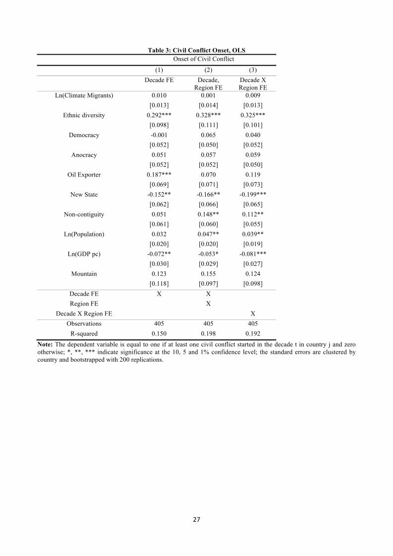
Table 3 presents the estimated parameters for conflict onset. This specification shows what makes a

"fresh" episode of violence start. The coefficients are almost invariant with respect to the conflict incidence

specification.

The variable climate-induced migrants has a non-statistically significant coefficient. The estimated

coefficient of the climate migrant, however, is potentially exposed to omitted-variable and reverse causality

biases. For example, countries experiencing a civil conflict may be a less attractive destination for migration.

To address such concern in the OLS estimates, we propose an instrumental variable strategy. To construct an

instrument for the climate-induced migration flows, we draw from the trade and migration literature. Frankel

and Romer (1999) and subsequently Rodriguez and Rodrik (2001), Rodrik et al. (2004) and Ortega and Peri

(2014) generate an instrument for trade flows by estimating a bilateral trade model using only geographic

characteristics as controls. Similarly, we compute an instrument by estimating a bilateral gravity equation:

14

𝑚#8,% = 𝛼 + 𝜃%% 𝐼% ∗ 𝑙𝑛𝐷#8 + 𝛽𝑙𝑛𝑃8MNOP + 𝛾𝐵#8 + 𝜓𝐿#8 + 𝜁𝐶#8 + 𝜓𝐴𝐸𝑍#8 + 𝜑% + 𝜑#% + 𝜖#8,% (4)

As in Frankel and Romer (1999) and the subsequent literature, once we have estimated the gravity

migration regression (6), we generate the fitted values for the log of bilateral migration flows for each pair of

countries in each year. We aggregate these predicted flows across destination j to compute the instrument for

the inflows of climate-induced migrants (𝐼𝑀).

Following the migration bilateral literature (Anderson, 2011; Beine et al., 2016; Beine et al., 2011;

Bertoli and Fernández-Huertas Moraga, 2013) the dependent variable 𝑚#8,% is the natural logarithm of

(climate-induced) migration flows from country c to destination j in decade t. The choice of the bilateral

geography controls to be included follows the standard in the literature. We take, however, only a small

subset of controls to avoid a violation of the exclusion restriction in the instrumental variable model. We use

the natural logarithm of population size in 1960 as a lagged measure (𝑃8MNOP), a dummy for whether the

origin and destination countries share a border (B), an official language (L), and colonial history (C). We add

a variable for the difference in Agro-Ecological Zones between origin and destination (EAZ), to capture the

extent to which migrants choose destinations with a climate similar to/different from the one of the origin

country.

Given that the geographic characteristics are time-invariant, to identify the evolution of bilateral

migration flows in time, we add time fixed effects and interactions between bilateral distance and time

dummies as in Feyrer (2009). These interactions should capture common advances in communication and

transportation that reduced the costs of migration. Being common to all countries, these shocks should be

exogenous with respect to any specific country. At the same time, they have different effects across country

pairs, as they depend on the relative pair distance. In particular, we add the natural logarithm of bilateral

(geodesic) distance interacted with decade dummies (I*lnD).

We also add a vector of decade fixed effects (𝜑%) and origin-decade fixed effects (𝜑#%) to account for

multilateral resistance, that arises from time varying common origin shocks to migration which influence

migrants' location decisions (Anderson and Van Wincoop, 2003; Bertoli and Fernández-Huertas Moraga,

2013; Ortega and Peri, 2013). Standard errors are clustered at the origin-destination pair level. To discard

potential sources of endogeneity bias, destination fixed effects are not included as they could absorb some

15

destination country characteristics that are correlated with conflicts. We run both OLS and a PPML (pseudo-

poisson maximum likelihood) estimators following Santos Silva and Tenreyro (2006). PPML estimator

addresses important heteroscedasticity and selection bias issues.

To mitigate concerns about the exclusion restrictions of the other geographic controls, we use only

bilateral and not unilateral geography variables in the gravity equation. Moreover, following Rodriguez and

Rodrik (2001) in the context of international trade, we include in the second-stage baseline model a set of

variables that should control for the main pathways between geography and conflicts. This is done in the

event that relative bilateral geography variables are correlated with absolute (unilateral) geography

characteristics, and thus may be correlated with conflicts. For this reason, we add in the conflict equation,

geography and disease variables, along with institutional quality.

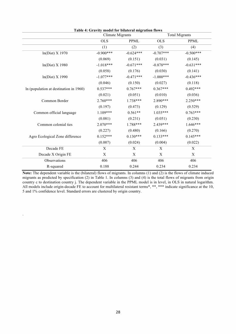
Table 4 reports the estimated parameters of PPML and OLS gravity models for environmental

migration. The point estimates are qualitatively comparable across the PPML and OLS models and have the

expected signs. Geographical distance is negatively correlated with bilateral climate-induced migration

flows, while linguistic links, common border and common colonial past are associated with larger migration

flows. Large destination economies tend to attract people. Interestingly, difference in the Agro Ecological

Zone between origin and destination boosts emigration, indicating that individuals tend to choose

destinations with a different climate.

We construct the instrument for climate-migrants using the fitted values of the log of bilateral

migration flows for each pair of countries in each year. Although we can compute predictions for both the

OLS and PPML gravity models, we will use only the predicted flows produced by the OLS model. Only the

OLS gravity based instrument proves to be a powerful instrument in the second stage, as indicated by the

reported F-tests.

Tables 5 and 6 show the 2SLS estimates of climate-induced migration on conflict incidence and

onset, respectively, which use the fitted values of the log of bilateral migration flows as an instrument in the

first stage regression. For the full sequence of columns, the tables have the structure described for Table 2.

The non-significant coefficient of climate-migrants is confirmed also by the 2SLS estimations. Based on this

finding, we cannot find empirical evidence of climate-migrants as an additional driver of tension in

destination countries. In the incidence specification, the positive and statistically significant coefficients of

16

ethnic diversity and population are robust to the 2SLS approach as well as the negative coefficient of GDP

per capita.

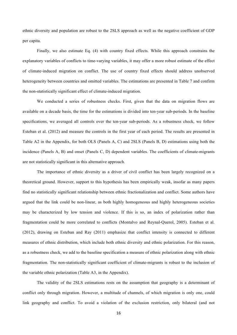
Finally, we also estimate Eq. (4) with country fixed effects. While this approach constrains the

explanatory variables of conflicts to time-varying variables, it may offer a more robust estimate of the effect

of climate-induced migration on conflict. The use of country fixed effects should address unobserved

heterogeneity between countries and omitted variables. The estimations are presented in Table 7 and confirm

the non-statistically significant effect of climate-induced migration.

We conducted a series of robustness checks. First, given that the data on migration flows are

available on a decade basis, the time for the estimations is divided into ten-year sub-periods. In the baseline

specifications, we averaged all controls over the ten-year sub-periods. As a robustness check, we follow

Esteban et al. (2012) and measure the controls in the first year of each period. The results are presented in

Table A2 in the Appendix, for both OLS (Panels A, C) and 2SLS (Panels B, D) estimations using both the

incidence (Panels A, B) and onset (Panels C, D) dependent variables. The coefficients of climate-migrants

are not statistically significant in this alternative approach.

The importance of ethnic diversity as a driver of civil conflict has been largely recognized on a

theoretical ground. However, support to this hypothesis has been empirically weak, insofar as many papers

find no statistically significant relationship between ethnic fractionalization and conflict. Some authors have

argued that the link could be non-linear, as both highly homogeneous and highly heterogeneous societies

may be characterized by low tension and violence. If this is so, an index of polarization rather than

fragmentation could be more correlated to conflicts (Montalvo and Reynal-Querol, 2005). Esteban et al.

(2012), drawing on Esteban and Ray (2011) emphasize that conflict intensity is connected to different

measures of ethnic distribution, which include both ethnic diversity and ethnic polarization. For this reason,

as a robustness check, we add to the baseline specification a measure of ethnic polarization along with ethnic

fragmentation. The non-statistically significant coefficient of climate-migrants is robust to the inclusion of

the variable ethnic polarization (Table A3, in the Appendix).

The validity of the 2SLS estimations rests on the assumption that geography is a determinant of

conflict only through migration. However, a multitude of channels, of which migration is only one, could

link geography and conflict. To avoid a violation of the exclusion restriction, only bilateral (and not

17

unilateral) geography variables are used in the gravity equation. Moreover, drawing on Rodriguez and

Rodrik (2001) and Ortega and Peri (2014) in the structural equation we account for the main channels

through which geography directly affects conflict. One potential pathway is represented by the type of

country institution, in that geography influences the quality of an institution and this strongly influences the

probability that a conflict occurs. We already account for this variable in the baseline specification.

Therefore, we also include a very broad set of geography and disease variables. These are controls for the

presence of yellow fever, absolute latitude, mean elevation above the sea level, average distance to the coast,

percent of land in the tropics, percent of population within 100 km from ice-free coast, percent of population

with malaria in 1994 and a landlocked dummy. Table A4, in the Appendix, presents the estimated results.

The coefficients of climate-migrants remain statistically non-significant.

The main objective of this paper is to estimate the effect of climate-induced migration on conflicts.

However, as the existing literature suggests, in addition to conflict potentially being caused by climate-

migrants, the own country’s climatic activity may lead to conflict as well. For this reason we add in the

conflict specification some controls for climate to reduce concerns about omitted variable bias. We use the

natural logarithm of average temperature and precipitation in the decade and the total number of extreme

events such as storm, flood, drought and extreme hit. The estimated coefficient of climate-migrants is still

statistically non-significant, as indicated in Table A5, in the Appendix. On the contrary, we find a robust,

positive and statistically significant coefficient of average temperature both on the incidence and onset of

civil conflicts. This finding is in agreement with the existing literature that finds a strong link between civil

war and temperature (Burke et al. 2009; Hsiang et al., 2013).

In the baseline specification we measure conflicts using the 25 deaths cut-off. This low threshold

ensures that even small and intermediate conflict events are captured. For robustness check and in agreement

with some of the existing literature, we use alternative definitions. First, we increase the minimum threshold

to 1000 or more battle deaths in a year, to capture the onset/existence of a war. Major conflicts such as wars

are of particular relevance, because of their critical damaging consequences. Second, given that a

dichotomous variable fails to utilize a lot of information on conflict, we also use a continuous variable for the

number of conflicts. We build a variable which counts all conflicting events involving more than 25 deaths

per year experienced by a country in a decade. Given the count nature of the dependent variable, we employ

18

a Poisson regression. Third, in line with Burke et al. (2009), Cotet and Tsui (2013), we employ military coup

attempts as a dependent variable. This variable records all successful, attempted, plotted and alleged coup

events without imposing any threshold.

The results of these alternative specifications are presented in Tables A6, A7 AND A8 in the

Appendix. The OLS coefficient of climate-migrants in the civil war incidence specification is negative and

statistically significant (Panel A, Table A6). This finding is likely connected to a reverse causality problem,

in that the existence of a large conflict at destination discourages the inflows of climate-migrants. Once the

reverse-causality is properly taken into account by a 2SLS estimation, the coefficient of climate-migrants

becomes zero (Panel B). In the civil war onset specification on the contrary, neither the OLS nor the 2SLS

coefficients of climate-migrants are statistically significant (Panels C and D). The null effect of climate-

migrants is robust to the use of a count variable for conflict (Table A7) or a coup attempt variable (Table

A8).

One could argue that the null effect of climate-induced international migration on conflict is due to

the strong control that leaders from receiving countries have over the borders. These strong controls may

constrain the inflow of migrants and reduce the possibility that climate-migrants induce conflicts at

destinations. An exception, however, might be represented by destination countries in Africa or South Asia,

where borders are more porous. For this reason in a robustness check we restrict the analysis to this subset of

destination countries. The empirical analysis for Africa and South Asia only are reported in Table A9. The

coefficient of climate-migrants is not statistically different from zero. It should be noted, however, that the F-

test for the power of the instrument in the first stage estimation is in some specifications smaller than the

value suggested by Staiger and Stock (1997) as a rule of thumb to assess the relevance of the instruments.

5. Conclusions

Human migration is an important response to environmental stress, but at the same time it could produce

substantial indirect effects. One such indirect effect could be the existence of a link between climate-induced

migration and conflicts. Competition over resources, ethnic tensions, distrust, demolition of social capital,

crossing of fault lines have been identified as possible bridging factors between conflicts and climate-

induced migration. In this paper, we test the possibility that climate change, through migration, could cause

19

new conflicts or fuel existing ones. A macro level empirical estimation is conducted to provide an answer to

this question.

Given that data on climate-migrants are not available, as the reasons for migration are not generally

recorded, we used an auxiliary regression to generate the number of migrants that are driven by climatic

factors, such as average temperature and precipitation, but also floods, droughts and storms. We also address

endogeneity concerns due to a reverse causality between migration and conflicts. The paper finds no

statistically significant effect of climate-migrants on conflicts. The result is robust to alternative

specifications, to alternative definitions of conflicts, whether onset or incidence, and to different thresholds

based on the number of deaths, to the inclusion of geographic and climate controls, and to the inclusion of

country fixed effects.

In this paper, we measure the incidence of these extreme events by counting the number of floods,

droughts and storms that occurred during the decade. The data used to capture these events come from the

EM-DAT, which however has some drawbacks. The data are mostly provided by insurance companies and

thus suffer from incomplete reporting, because small events or events occurring in poor countries are under-

sampled. This problem is particularly serious before 1990, which is the period where a large part of the

present analysis is conducted. This limitation could partially explain why climate migrants do not increase

the risk of civil conflict in this study.

Moreover, destination countries have effective policies of land allocation and dispute resolution that

prevent the rise of civil conflicts. This could be an additional reason explaining why climate-migrants are not

responsible for increasing disputes. That said, it could be the case that even if a destination country does not

experience civil conflicts, characterized by a certain number of battle-related deaths, it may be susceptible to

less intense social unrest or to a larger number of crimes due to climate-migrants.

Another limitation of the present study is that it considers only international migration. This type of

migration is only a fraction of the total and could differ from internal moves from a variety of aspects,

including the income and skills profiles of those who leave. Internally displaced persons could have a

different effect on conflicts given that they tend to be poorer and unskilled and boost urbanization without

growth. This may explain why the findings of this paper differ from the results of Ghimire at al. (2015),

20

where a causal link between the number of people internally displaced by large floods and civil conflict is

reported.

Finally, it is also possible that when population density increases as a result of migrant inflows,

agriculture begins to intensify. Migrants can contribute to this technology shift by bringing new knowledge

and skills. This process may introduce an additional channel between migration and conflict, which offsets

the potential negative impact of land scarcity. Two forces, one leading to an increase in economic efficiency

and the other causing higher competition over resources may work in opposite directions and explain the null

effect of climate migrants of this paper. The analysis of potential benefit of climate-induced migration could

represent a possible future extension of the present paper.

Migration is an important instrument of adaptation to climate change. At the same time it is crucial to

promote other forms of adaptation by increasing the access to energy, improving the efficiency of

agricultural production and the water supply systems. Alternative ways to cope with climate change are

needed, as migration cannot be the single solution to address climate-related risks. This is particularly

important as the indirect impacts of climatic stress through massive migration could be as substantial as the

direct ones.

21

6. References

Anderson J. E. (2011) “The Gravity Model” Annual Review of Economics, 3, pp. 133-160

Anderson, J. and E. Van Wincoop (2003) "Gravity And Gravitas: A Solution To The Border Puzzle" American Economic Review, vol. 93(1), pp. 170-192

Balk D. et al. (2004) Global Rural-Urban Mapping Project (GRUMP), Palisades, NY: CIESIN, Columbia University. Available at http://sedac.ciesin.columbia.edu/gpw

Barrios, S.,L., Bertinelli, and E., Strobl (2006),"Climatic change and rural-urban migration: The case of sub-Saharan Africa," Journal of Urban Economics, vol.60(3), 357-371

Beine M., F. Docquier and Ç. Özden, (2011) "Diasporas," Journal of Development Economics, 95(1), pp. 30-41

Beine M., Si. Bertoli and J. Fernández-Huertas Moraga (2015) “A Practitioners’ Guide to Gravity Models of International Migration” The World Economy, 39(4), pp.496–512

Beine M. and C. Parsons (2015) “Climatic Factors as Determinants of International Migration”, Scandinavian Journal of Economics, 117(2), pp 7

Berman N., M. Couttenier, D. Rohner and M. Thoenig (2017) “This mine is mine! How minerals fuel conflicts in Africa” forthcoming American Economic Review

Bertoli, S. and J. Fernández-Huertas Moraga (2013) "Multilateral Resistance to Migration" Journal of Development Economics, vol. 102, pp. 79-100

Black R., S. Bennett, S. Thomas, J. Beddington (2011). “Climate Change: Migration as Adaptation.” Nature 478, 447-449.

Borjas G. J. (1987) “Self-Selection and the Earnings of Immigrants" The American Economic Review. 77(4): 531-553

Buhaug, H. (2010) “Climate Not to Blame for African Civil Wars” Proceedings of the National Academy of Sciences, 107 (38), 16477-16482

Burke M. B., E. Miguel, S. Satyanath, J. A. Dykema, and D.B. Lobell (2009) “Warming Increases the Risk of Civil War in Africa” Proceedings of the National Academy of Sciences, 106(37), 20670-20674

Cai R., S. Feng, M. Pytlikova and M. (2016) " Climate variability and international migration: The importance of the agricultural linkage” Journal of Environmental Economics and Management, 79, pp. 135–151

Cattaneo C. and G. Peri (2016) “The Migration Response to Increasing Temperatures” Journal of Development Economics, 122, pp. 127-146

Cattaneo C., C. Fiorio and G. Peri (2015) “What Happens to the Careers of European Workers When Immigrants "Take Their Jobs”, Journal of Human Resources, vol. 50(3), pp. 655-693

Ciccone (2011) “Economic shocks and civil conflicts: a comment” American Economic Journal: Applied Economics”, 3, 215-227

Collier P. and A. Hoeffler (2002) “Greed and grievance in civil war” Oxford Economic Papers, 56, pp. 563-595

Cotet A. M., and K. K. Tsui (2013) “Oil and Conflict: What Does the Cross Country Evidence Really Show?” American Economic Journal: Macroeconomics , 5(1), 49-80

Couttenier M. and R. Soubeyran (2014) “Drought and Civil War In Sub-Saharan Africa” Economic Journal, 124(575), pp. 201-244

Dell M., B. Jones and B. Olkien (2012) "Temperature Shocks and Economic Growth: evidence from the last half Century" American Economic Journal: Macroeconomics, 4(3), pp 66-95

22

Esteban J. and D. Ray (2011) “Linking Conflict to Inequality and Polarization”, American Economic Review, 101(4), pp. 1345-1374

Esteban J., L. Mayoral and D. Ray (2012) “Ethnicity and Conflict: an empirical Study” American Economic Review, 102(4), 1310-1342

Esteban J., M. Morelli and D. Rohner (2015) “Strategic Mass Killing” Journal of Political Economy, 123(5), 1087-1132

Fearon J. and D. Laitin (2003) “Ethnicity, insurgency, and civil war” American Political Science Review, vol. 97, pp. 75–90

Feyrer J. (2009) “Trade and Income --Exploiting Time Series in Geography” NBER Working Paper No. 14910

Frankel J. and D. Romer (1999) "Does Trade Cause Growth?", American Economic Review, 89(3), pp 379-399

Fussell, E., L. Hunter, C. Gray (2014). “Measuring the Environmental Dimensions of Human Migration: The Demographer’s Toolkit.” Global Environmental Change 28: 182-191

Ghimire R., S. Ferreira and J. Dorfman (2015) “Flood-induced displacement and civil conflict” World Development, 66, 614-628

Guha-Sapir D., R. Below, P. Hoyois (2015) EM-DAT: The CRED/OFDA International Disaster Database – www.emdat.be – Université Catholique de Louvain – Brussels – Belgium

Harari M. and E. La Ferrara (2014) “Conflict, Climate and Cells: A Disaggregated Analysis” IGIER Working Paper n. 461

Heston, Alan, Robert Summers, and Bettina Aten (2011): "PennWorld Table Version 7.0", dataset, Center for International Comparisons of Production, Income and Prices at the University of Pennsylvania

Hsiang, S.M., K. Meng and M. Cane (2011) “Civil conflicts are associated with the global climate”, Nature, 476, 438-441

Hsiang, S.M., Burke, M., and Miguel, E. (2013). Quantifying the Influence of Climate on Human Conflict. Science, 341:1235367

IPCC (2014) Climate Change 2014: Impacts, Adaptation, and Vulnerability. Contribution of Working Group II to the Fifth Assessment Report of the Intergovernmental Panel on Climate Change. Cambridge University Press, Cambridge, United Kingdom and New York, NY, USA

Jones B. and B. A. Olken (2010) "Climate Shocks and Exports" American Economic Review, vol. 100(2), pages 454-59

Marchiori, L., J-F. Maystadt and I. Schumacher (2011) “The Impact of Weather Anomalies on Migration in Sub-Saharan Africa”, Journal of Environmental Economics and Management, 63(3), 355-374

Matsuura K., and C. J. Willmott (2007) “Terrestrial Air Temperature and Precipitation: 1900-2006 Gridded Monthly Time Series, Version 1.01" http://climate.geog.udel.edu/~climate/

Miguel, E., S. Satyanath, and E. Sergenti (2004) “Economic Shocks and Civil Conflict: An Instrumental variables Approach” Journal of Political Economy, 112, 725-753

Montalvo J. and M. Reynol-Querol (2005) "Ethnic Polarization, Potential Conflict, and Civil Wars", Economic Journal, 95(3), pp. 796-816

Montalvo J. and M. Reynol-Querol (2008). "Discrete Polarisation with an Application to the Determinants of Genocides", Economic Journal, 118, pp. 1835-65

Morelli and Rohner (2015) “Resource Concentration and Civil War” Journal of Development Economics, vol. 117, pp. 32-47

Ortega, F. and G. Peri (2013) “The Effect of Income and Immigration Policies on International Migration.” Migration Studies, 1, pp. 1-28

23

Ortega F. and G. Peri (2014) “Openness and Income: the roles of trade and migration”, Journal of International economics, 92, pp. 231-251

Özden C., C. R. Parsons, M. Schiff and T L. Walmsley (2011) “Where on Earth is Everybody? The Evolution of Global Bilateral Migration 1960–2000”, World Bank Economic Review, 25(1), 12-56

Pagan A. (1984) “Econometric Issues in the Analysis of Regressions with Generated Regressors” International Economic Review, 25(1), pp. 221-247

Peri G. (2005) "Determinants of Knowledge Flows and Their Effect on Innovation," The Review of Economics and Statistics, 87(2), pp. 308-322

Reuveny R. (2007) “Climate change induced migration and violent conflicts”, Political Geography, 26, pp. 656-673

Rodriguez, F., Rodrik, D., (2001) “Trade policy and economic growth: a skeptic's guide to the cross-national evidence. NBER Macroeconomics Annual, vol. 15, pp. 261–338

Rodrik D., A. Subramanian and F. Trebbi (2004) “Institutions Rule: The Primacy of Institutions Over Geography and Integration in Economic Development, Journal of Economic Growth, 9(2), pp 131–165

Roy, A.D. (1951) “Some thoughts on the distribution of earnings" Oxford Economic Papers, vol.3(2), pp 135-46

Santos-Silva J. and S. Tenreyro (2006) “The log of gravity” Review and Economic and Statistics, 88(4), pp. 641-658

Sassen S. (2014) Expulsions: Brutality and Complexity in the Global Economy. Cambridge, MA: Belknap Press of Harvard University Press

Staiger D. and J. H. Stock (1997) “Instrumental variables regression with weak instruments” Econometrica, 65, pp. 557–586

Withagen C. (2014) “The climate change, migration and conflict nexus”, Environment and Development Economics, 19(3), pp. 324-327

Wooldridge J. (2010) Econometric Analysis of Cross Section and Panel Data. 2 edition, MIT Press Books, The MIT Press

World Bank (2016) World Development Indicators. http://data.worldbank.org/data-catalog/world-development-indicators

24

Tables and Figures

Figure 1: Total and Climate-Induced Outflows of Migrants per capita

Notes: the graph displays the scatterplot of the average outflows of migrants per capita and the average outflows of climate induced migrants per capita. The climate induced migrants are predicted using specification (2) of Table 1.

02

46

810

Tota

l Mig

rant

s pe

r cap

ita

0 .5 1 1.5 2Climate Migrants per capita

25

Table 1: Temperature effects for different groups of countries Net emigration flows

(1) (2) Temperature*middle income dummy 1.871 1.608

(2.697) (2.724) Precipitation*middle income dummy -7.181** -7.392**

(3.028) (3.002) Drought*middle income dummy 21.688 22.425

(29.242) (29.333) Flood*middle income dummy 16.209** 16.564**

(7.413) (7.399) Storm*middle income dummy 17.210** 17.102**

(8.446) (8.492) Temperature*low income dummy 1.058 1.024

(2.235) (2.287) Precipitation* low income dummy -3.767* -3.957*

(1.925) (2.018) Drought* low income dummy 9.278 7.306

(13.229) (13.724) Flood* low income dummy -2.455 -1.620

(4.170) (4.185) Storm* low income dummy 1.695 2.559

(6.178) (6.274) Temperature*high income dummy -3.772 -0.842

(2.739) (2.968) Precipitation* high income dummy -0.872 0.064

(3.046) (3.108) Drought* high income dummy -62.195*** -70.736***

(21.095) (20.869) Flood* high income dummy 16.435** 15.461**

(6.444) (6.315) Storm* high income dummy -0.276 -0.014

(1.767) (1.744) Decade X Region FE X X

Decade X High Income FE X Observations 614 614

R-squared 0.309 0.313

Note: The dependent variable is the emigration flows (divided by 1000). The standard errors are clustered by country of origin. *, **, *** indicate significance at the 10, 5 and 1% confidence level.

26

Table 2: Civil Conflict Incidence, OLS Incidence of Civil Conflict

(1) (2) (3) Decade FE Decade,

Region FE Decade X Region FE

Ln(Climate Migrants) 0.010 0.001 0.010 [0.015] [0.015] [0.014]

Ethnic diversity 0.267* 0.371** 0.349*** [0.137] [0.152] [0.129]

Democracy 0.006 0.064 0.049 [0.059] [0.064] [0.063]

Anocracy 0.074 0.066 0.072 [0.066] [0.064] [0.064]

Oil Exporter 0.179** 0.027 0.088 [0.079] [0.088] [0.081]

New State -0.136* -0.130 -0.168* [0.081] [0.084] [0.098]

Non-contiguity 0.080 0.197** 0.147* [0.089] [0.093] [0.077]

Ln(Population) 0.045 0.059** 0.051** [0.027] [0.026] [0.026]

Ln(GDP pc) -0.117*** -0.111*** -0.139*** [0.039] [0.042] [0.037]

Mountain 0.109 0.109 0.087 [0.136] [0.125] [0.111]

Decade FE X X Region FE X

Decade X Region FE X Observations 405 405 405

R-squared 0.189 0.246 0.237

Note: The dependent variable is equal to one if at least one civil conflict was ongoing in the decade t in country j and zero otherwise; *, **, *** indicate significance at the 10, 5 and 1% confidence level; the standard errors are clustered by country and bootstrapped with 200 replications.

27

Table 3: Civil Conflict Onset, OLS Onset of Civil Conflict




Ethnic diversity 0.292*** 0.328*** 0.325*** [0.098] [0.111] [0.101]

Democracy -0.001 0.065 0.040 [0.052] [0.050] [0.052]

Anocracy 0.051 0.057 0.059 [0.052] [0.052] [0.050]

Oil Exporter 0.187*** 0.070 0.119 [0.069] [0.071] [0.073]

New State -0.152** -0.166** -0.199*** [0.062] [0.066] [0.065]

Non-contiguity 0.051 0.148** 0.112** [0.061] [0.060] [0.055]

Ln(Population) 0.032 0.047** 0.039** [0.020] [0.020] [0.019]

Ln(GDP pc) -0.072** -0.053* -0.081*** [0.030] [0.029] [0.027]

Mountain 0.123 0.155 0.124 [0.118] [0.097] [0.098]



R-squared 0.150 0.198 0.192

Note: The dependent variable is equal to one if at least one civil conflict started in the decade t in country j and zero otherwise; *, **, *** indicate significance at the 10, 5 and 1% confidence level; the standard errors are clustered by country and bootstrapped with 200 replications.

28

Table 4: Gravity model for bilateral migration flows Climate Migrants Total Migrants OLS PPML OLS PPML (1) (2) (3) (4)

ln(Dist) X 1970 -0.900*** -0.624*** -0.707*** -0.500*** (0.069) (0.151) (0.031) (0.145)

ln(Dist) X 1980 -1.018*** -0.671*** -0.878*** -0.631*** (0.058) (0.176) (0.030) (0.141)

ln(Dist) X 1990 -1.077*** -0.471*** -1.000*** -0.436*** (0.046) (0.150) (0.027) (0.118)

ln (population at destination in 1960) 0.537*** 0.767*** 0.367*** 0.492*** (0.021) (0.051) (0.010) (0.036)

Common Border 2.760*** 1.738*** 2.890*** 2.250*** (0.197) (0.473) (0.129) (0.529)

Common official language 1.109*** 0.561** 1.035*** 0.763*** (0.081) (0.231) (0.051) (0.230)

Common colonial ties 2.070*** 1.788*** 2.439*** 1.646*** (0.227) (0.480) (0.166) (0.270)

Agro Ecological Zone difference 0.152*** 0.130*** 0.133*** 0.145*** (0.007) (0.024) (0.004) (0.022)

Decade FE X X X X Decade X Origin FE X X X X

Observations 406 406 406 406 R-squared 0.188 0.244 0.234 0.234

Note: The dependent variable is the (bilateral) flows of migrants. In columns (1) and (2) is the flows of climate induced migrants as predicted by specification (2) in Table 1. In columns (3) and (4) is the total flows of migrants from origin country c to destination country j. The dependent variable in the PPML model is in level, in OLS in natural logarithm. All models include origin-decade FE to account for multilateral resistant terms*, **, *** indicate significance at the 10, 5 and 1% confidence level. Standard errors are clustered by origin country.

.

29

Table 5: Civil Conflict Incidence, 2SLS Incidence of Civil Conflict



Ln(Climate Migrants) -0.008 -0.012 -0.013 [0.043] [0.054] [0.047]

Ethnic diversity 0.285* 0.384*** 0.370*** [0.151] [0.148] [0.135]

Democracy 0.006 0.069 0.051 [0.057] [0.078] [0.065]

Anocracy 0.072 0.067 0.074 [0.064] [0.069] [0.067]

Oil Exporter 0.178** 0.022 0.083 [0.073] [0.091] [0.067]

New State -0.124 -0.123 -0.155 [0.079] [0.088] [0.100]

Non-contiguity 0.085 0.197** 0.146 [0.091] [0.092] [0.090]

Ln(Population) 0.055 0.067* 0.064* [0.035] [0.038] [0.033]

Ln(GDP pc) -0.099* -0.100 -0.118** [0.055] [0.065] [0.057]

Mountain 0.102 0.104 0.080 [0.130] [0.143] [0.136]



R-squared 0.185 0.244 0.231 First Stage F-Stat 22.43 20.67 18.92

Note: The dependent variable is equal to one if at least one civil conflict was ongoing in the decade t in country j and zero otherwise; *, **, *** indicate significance at the 10, 5 and 1% confidence level; the standard errors are clustered by country and bootstrapped with 200 replications.

30

Table 6: Civil Conflict Onset, 2SLS Onset of Civil Conflict




Ethnic diversity 0.306*** 0.334*** 0.337*** [0.088] [0.108] [0.104]

Democracy -0.001 0.067 0.041 [0.055] [0.061] [0.057]

Anocracy 0.049 0.057 0.060 [0.053] [0.052] [0.052]

Oil Exporter 0.186*** 0.067 0.116* [0.070] [0.074] [0.069]

New State -0.143** -0.163** -0.192** [0.060] [0.074] [0.077]

Non-contiguity 0.055 0.148** 0.112* [0.061] [0.072] [0.066]

Ln(Population) 0.040 0.050* 0.046* [0.028] [0.030] [0.025]

Ln(GDP pc) -0.059 -0.048 -0.070* [0.039] [0.049] [0.042]

Mountain 0.119 0.153 0.120 [0.120] [0.097] [0.107]



R-squared 0.147 0.197 0.190 First Stage F-Stat 22.43 20.67 18.92

Note: The dependent variable is equal to one if at least one civil conflict started in the decade t in country j and zero otherwise; *, **, *** indicate significance at the 10, 5 and 1% confidence level; the standard errors are clustered by country and bootstrapped with 200 replications.

31

Table 7: Civil Conflict, country fixed effects (1) Panel A: Civil Conflict Incidence (OLS)

Ln(Climate Migrants) -0.004 [0.020] Panel B: Civil Conflict Incidence (2SLS)

Ln(Climate Migrants) 0.015 [0.053]

First Stage F-stat 51.11 Panel C: Civil Conflict Onset (OLS)

Ln(Climate Migrants) 0.009 [0.022] Panel D: Civil Conflict Onset (2SLS)

Ln(Climate Migrants) 0.023 [0.063]

First Stage F-stat 51.11 Country FE X

Decade X Region FE X Observations 411

Note: The dependent variable is equal to one if at least one civil conflict was ongoing in the decade t in country j and zero otherwise in Panels (a) and (b); it is equal to one if at least one civil conflict started in the decade t in country j and zero otherwise in Panels (c) and (d); *, **, *** indicate significance at the 10, 5 and 1% confidence level; the standard errors are clustered by country and bootstrapped with 200 replications.

32

Appendix A: Additional Regression Tables

Table A1: Summary Statistics

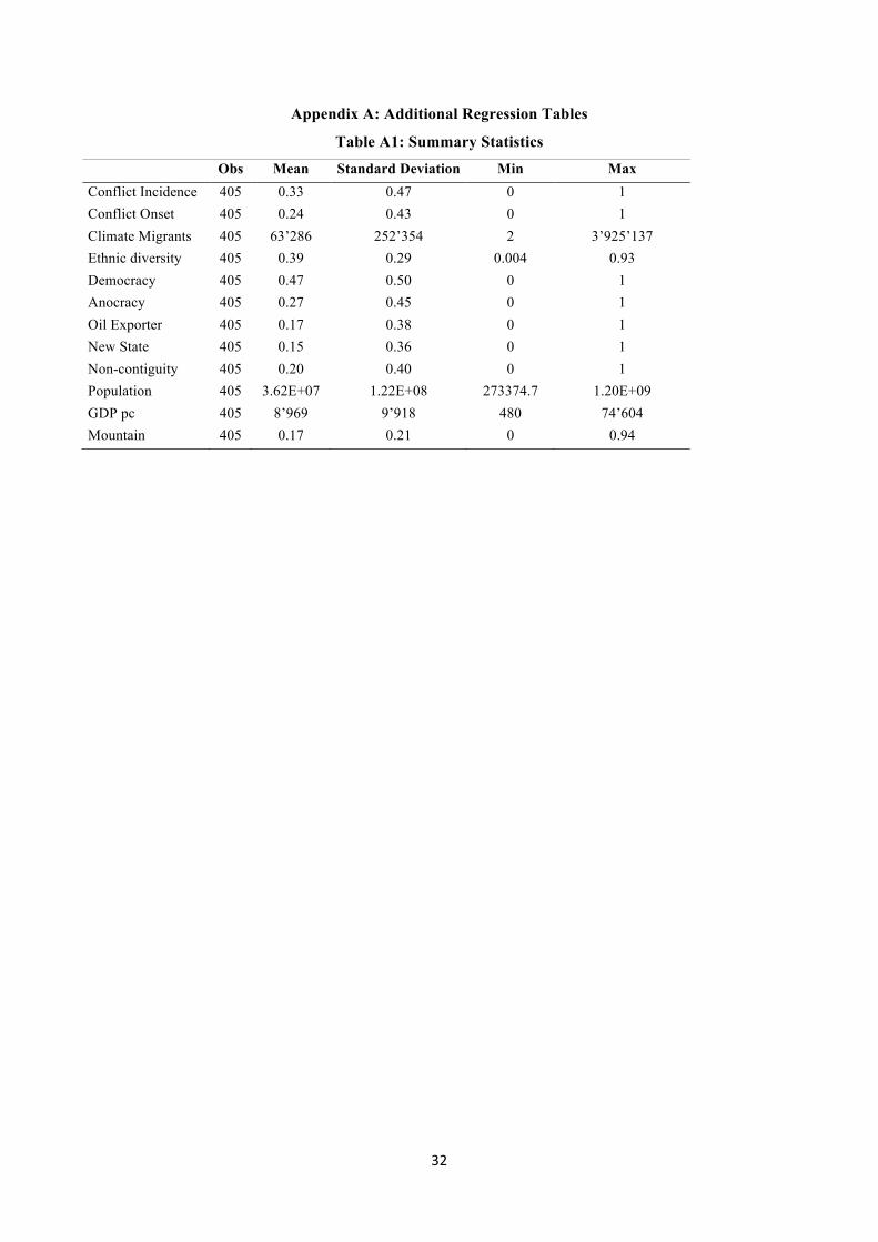
Obs Mean Standard Deviation Min Max Conflict Incidence 405 0.33 0.47 0 1 Conflict Onset 405 0.24 0.43 0 1 Climate Migrants 405 63’286 252’354 2 3’925’137 Ethnic diversity 405 0.39 0.29 0.004 0.93 Democracy 405 0.47 0.50 0 1 Anocracy 405 0.27 0.45 0 1 Oil Exporter 405 0.17 0.38 0 1 New State 405 0.15 0.36 0 1 Non-contiguity 405 0.20 0.40 0 1 Population 405 3.62E+07 1.22E+08 273374.7 1.20E+09 GDP pc 405 8’969 9’918 480 74’604 Mountain 405 0.17 0.21 0 0.94

33

Table A2: Civil Conflict, controls at the beginning of the decade (1) (2) (3)

Decade FE Decade, Region FE Decade X Region Panel A: Civil Conflict Incidence (OLS)

Ln(Climate Migrants) 0.005 -0.005 0.004 [0.015] [0.014] [0.013] Panel B: Civil Conflict Incidence (2SLS)


First Stage F-stat 20.49 20.83 16.71 Panel C: Civil Conflict Onset (OLS)

Ln(Climate Migrants) 0.010 0.001 0.010 [0.012] [0.013] [0.013] Panel D: Civil Conflict Onset (2SLS)


First Stage F-stat 20.49 20.83 16.71 Country FE X X

Decade X Region FE X X Observations 385 385 385


34

Table A3: Civil Conflict, control for polarization (1) (2) (3)






Ln(Climate Migrants) 0.001 -0.004 0.007 [0.046] [0.047] [0.048]




35

Table A4: Civil Conflict, controls for geography (1) (2) (3)









Note: The dependent variable is equal to one if at least one civil war was ongoing in the decade t in country j and zero otherwise in Panels (a) and (b); it is equal to one if at least one civil war started in the decade t in country j and zero otherwise in Panels (c) and (d); *, **, *** indicate significance at the 10, 5 and 1% confidence level; the standard errors are clustered by country and bootstrapped with 200 replications.

36

Table A5: Civil Conflict, controls for climate (1) (2) (3)


Ln(Climate Migrants) 0.001 0.001 0.005 [0.013] [0.014] [0.015] Panel B: Civil Conflict Incidence (2SLS)








37

Table A6: Civil War (1) (2) (3)

Decade FE Decade, Region FE Decade X Region Panel A: Civil War Incidence (OLS)

Ln(Climate Migrants) -0.025* -0.029* -0.023 [0.014] [0.015] [0.015] Panel B: Civil War Incidence (2SLS)


First Stage F-stat 22.43 20.67 18.92 Panel C: Civil War Onset (OLS)

Ln(Climate Migrants) -0.009 -0.011 -0.009 [0.008] [0.010] [0.008] Panel D: Civil War Onset (2SLS)




Note: The dependent variable is equal to one if at least one civil war was ongoing in the decade t in country j and zero otherwise in Panels (a) and (b); it is equal to one if at least one civil war started in the decade t in country j and zero otherwise in Panels (c) and (d); *, **, *** indicate significance at the 10, 5 and 1% confidence level; the standard errors are clustered by country and bootstrapped with 200 replications.

Table A7: Number of conflicts in the decade

(1) (2) (3)

Decade FE Decade, Region FE Decade X Region Panel A: Number of conflicts (OLS)

Ln(Climate Migrants) -0.091 -0.083 -0.066 [0.079] [0.076] [0.074] Panel B: Number of conflicts (2SLS)

Ln(Climate Migrants) -0.063 0.029 -0.042 [0.170] [0.180] [0.114]



Note: The dependent variable is the count of the civil conflicts in a decade; *, **, *** indicate significance at the 10, 5 and 1% confidence level; the standard errors are bootstrapped with 200 replications. Given the count nature of the dependent variable, a Poisson regression is employed.

38

Table A8: Coup

(1) (2) (3)

Decade FE Decade, Region FE Decade X Region Panel A: Coup (OLS)

Ln(Climate Migrants) 0.099 0.082 0.061 [0.121] [0.132] [0.122] Panel B: Coup (2SLS)




Note: The dependent variable is military coup attempts; *, **, *** indicate significance at the 10, 5 and 1% confidence level; the standard errors are clustered by country and bootstrapped with 200 replications.

Table A9: Civil Conflict, only Africa and Asia (1) (2) (3)


Ln(Climate Migrants) 0.009 0.011 0.012 [0.025] [0.025] [0.024] Panel B: Civil Conflict Incidence (2SLS)








39

Appendix B: List of countries in the conflict specification

Afghanistan, Albania, Angola, Argentina, Australia, Austria, Bahrain, Bangladesh, Benin, Bhutan, Bolivia,

Botswana, Brazil, Bulgaria, Burkina Faso, Burundi, Cambodia, Cameroon, Canada, Central African

Republic, Chad, Chile, China, Colombia, Congo, Democratic Republic of the Congo, Costa Rica, Cote

d'Ivoire, Cuba, Cyprus, Denmark, Djibouti, Dominican Republic, Ecuador, Egypt, El Salvador, Ethiopia,

Fiji, Finland, France, Gabon, Gambia, Germany, Ghana, Greece, Guatemala, Guinea, Guinea-Bissau,

Guyana, Haiti, Honduras, India, Indonesia, Iran, Iraq, Ireland, Israel, Italy, Jamaica, Japan, Jordan, Kenya,

Republic of Korea, Kuwait, Lao People's Democratic Republic, Lebanon, Lesotho, Liberia, Libya,

Madagascar, Malawi, Malaysia, Mali, Mauritania, Mauritius, Mexico, Mongolia, Mozambique, Nepal,

Netherlands, New Zealand, Nicaragua, Niger, Nigeria, Norway, Oman, Pakistan, Panama, Papua New

Guinea, Paraguay, Peru, Philippines, Poland, Portugal, Romania, Rwanda, Saudi Arabia, Senegal, Sierra

Leone, Singapore, Somalia, South Africa, Spain, Sri Lanka, Sudan, Swaziland, Sweden, Switzerland, Syria,

Tanzania, Thailand, Togo, Trinidad and Tobago, Tunisia, Turkey, Uganda, United Arab Emirates, United

Kingdom, United States of America, Uruguay, Venezuela, Viet Nam, Yemen, Zambia

List of high income countries in the migration specification

Argentina, Australia, Austria, Bahamas, Belgium, Brunei, Canada, Chile, Cyprus, Denmark, Equatorial

Guinea, Finland, France, Germany, Greece, Hungary, Iceland, Ireland, Israel, Italy, Japan, Republic of

Korea, Kuwait, Luxembourg, Netherlands, New Zealand, Norway, Oman, Poland, Portugal, Qatar, Saudi

Arabia, Spain, Sweden, Switzerland, Taiwan, Trinidad and Tobago, United Arab Emirates, United Kingdom,

United States, Uruguay, Venezuela

List of middle income countries in the migration specification

Albania, Algeria, Angola, Bangladesh, Belize, Bhutan, Bolivia, Botswana, Brazil, Bulgaria, Cameroon, Cape

Verde, China, Colombia, Republic of Congo, Costa Rica, Cote d`Ivoire, Cuba, Djibouti, Dominican

Republic, Ecuador, Egypt, El Salvador, Fiji, Gabon, Ghana, Guatemala, Guyana, Honduras, India, Indonesia,

Iran, Iraq, Jamaica, Jordan, Kenya, Laos, Lebanon, Lesotho, Libya, Malaysia, Mauritania, Mauritius,

Mexico, Mongolia, Morocco, Myanmar, Namibia, Nicaragua, Nigeria, Pakistan, Panama, Papua New

Guinea, Paraguay, Peru, Philippines, Romania, Samoa, Sao Tome and Principe, Senegal, Solomon Islands,

South Africa, Sri Lanka, St. Vincent and Grenadines, Sudan, Suriname, Swaziland, Syria, Thailand, Tunisia,

Turkey, Vanuatu, Vietnam, Yemen, Zambia

List of low income countries in the migration specification

Afghanistan, Benin, Burkina Faso, Burundi, Cambodia, African Republic, Chad, Comoros, Dem. Rep.

Congo, Ethiopia, Gambia, Guinea, Guinea-Bissau, Haiti, Dem. Rep. Korea, Liberia, Madagascar, Malawi,

Mali, Mozambique, Nepal, Niger, Rwanda, Sierra Leone, Somalia, Tanzania, Togo, Uganda, Zimbabwe

40

Appendix C: Data description and sources

Conflict Incidence: dummy variable equal to one if at least one civil conflict occurred in the decade t. Data

are taken from UCDP/PRIO Armed Conflict Dataset

Conflict Onset: dummy variable equal to one if at least one civil conflict started in the decade t. Data are

taken from UCDP/PRIO Armed Conflict Dataset

Climate migrants: climate-induced net immigration flows, predicted from Eq. 2. Data on flows of migrants

are taken from Ozden et al. (2011).

Ethnic diversity: Index of ethnic fractionalization. From Fearon and Laitin (2003).

Democracy: Dummy variable equal to 1 if the Polity scores from Polity IV (2012) is greater than six.

Anocracy: Dummy variable equal to 1 if the Polity scores from Polity IV (2012) is lower than minus six.

Oil Exporter: Dummy variable taking a value of 1 if in a given country and year the fuel exports (in % of

merchandise exports) is above 33%. Variable from Morelli and Rohner (2015)

New State: Dummy variable taking a value of 1 if a state was created in the previous 10 years, coded as 0

otherwise.

Non-contiguity: Dummy taking a value of 1 if a state has noncontiguous territory. From Fearon and Laitin

(2003).

Ln(Population): Total population. From World Bank (2016).

Ln(GDP pc): PPP adjusted GDP per capita at constant prices. From the Penn World Tables (Heston,

Summers, and Aten, 2011).

Mountain: Percentage of territory covered by mountains. From Morelli and Rohner (2015)

Climate-induced international migration and conflicts

41

Fond

azio

ne C

entr

o Eu

ro-M

edite

rran

eo s

ui C

ambi

amen

ti C

limat

ici

© Fondazione CMCC - Centro Euro-Mediterraneo sui Cambiamenti Climatici 2017 Visit www.cmcc.it for information on our activities and publications.

The Foundation Euro-Mediterranean Centre on Climate Change has its registered office and administration in Lecce and other units in Bologna, Venice, Capua, Sassari, Viterbo and Milan. The CMCC Foundation doesn’t pursue profitable ends and aims to realize and manage the Centre, its promotion, and research coordination and different scientific and applied activities in the field of climate change study.

rp0284 – climate-induced international migration and · rp0284 – climate-induced international...

Documents