routes to chaos in neural networks with random weights

Papers

International Journal of Bifurcation and Chaos, Vol. 8, No. 7 (1998) 1463–1478c© World Scientific Publishing Company

ROUTES TO CHAOS IN NEURAL NETWORKSWITH RANDOM WEIGHTS

D. J. ALBERS and J. C. SPROTTDepartment of Physics, University of Wisconsin, Madison,

1150 University Avenue, Madison, WI 53706, USA

W. D. DECHERTDepartment of Economics, University of Houston,

Houston TX 77204-5882, USA

Received January 13, 1998; Revised May 9, 1998

Neural networks are dense in the space of dynamical systems. We present a Monte Carlo studyof the dynamic properties along the route to chaos over random dynamical system functionspace by randomly sampling the neural network function space. Our results show that asthe dimension of the system (the number of dynamical variables) is increased, the probabilityof chaos approaches unity. We present theoretical and numerical results which show that asthe dimension is increased, the quasiperiodic route to chaos is the dominant route. We alsoqualitatively analyze the dynamics along the route.

1. Introduction

The study of complex systems over the past fewdecades has led to many interesting and diverse re-sults. The dynamics encountered in many differ-ent systems occurs across diverse disciplines. Thisapparent similarity in dynamics has motivated ourMonte Carlo study of dynamical systems using neu-ral networks, since neural networks are dense inthe set of continuous functions on a bounded in-terval. We investigate the general dynamic prop-erties, including the probability of chaos, and thepower spectrum. As the dimension is increased,the probability of chaos approaches unity. Withthis in mind, we study the route to chaos as theconnection strengths are increased. Numerically wefind that as the dimension is increased the proba-bility of the first bifurcation being Hopf increases tonear unity. Based on observing the bifurcation dia-grams of hundreds of networks, we conject that thequasiperiodic route dominates at high dimension.Besides the evidence and conjectures put forth byDoyon et al., [1993] and Brock [1997] regarding very

general systems, there is evidence that some spe-cialized systems such as coupled map lattices andcoupled identical period-doubling systems also tendto, or do undergo the quasiperiodic route to chaos[Wang & Cerdeira, 1996; Reick & Mosekilde, 1995].

2. Bifurcation Theory andChaotic Dynamics

Define X to be an open subset of a Banach space,E. Next set I = [a, b] ∈ R. Now define the mapfµ : X 7→ E for µ ∈ I, thus forming a param-eterized family of maps for which µ is the bifur-cation parameter. Define µ0 ∈ I such that fµ0

has a fixed point at x0 ∈ X. Define Γ such thatΓ = {(µ, x) ∈ I × X : fµx = x}. Now, supposethat (µ0, x0) ∈ Γ, where x0 is not hyperbolic. Abifurcation occurs where Dx0fµ0 has a eigenvalueon the unit circle. There are three generic waysthis can occur, (and hence three generic bifurca-tions): Flip, where a negative real eigenvalue lieson the unit circle (Dx0fµ0 = −1), (this correspondsto a period-two oscillation); saddle-node, where

1463

1464 D. J. Albers et al.

a positive real eigenvalue lies on the unit circle(Dx0fµ0 = 1), (this corresponds to the appearanceof two branches of stable equilibria); and Hopf,1

where a complex conjugate pair of eigenvalues lieon the unit circle (Dx0fµ0 = |a ± bi| = 1, b 6= 0),(this corresponds to the appearance of a limit cycleor torus). The three types of bifurcations describedabove are generic when Γ is a nonsingular smoothcurve. We have yet to impose any symmetry groups,but it should be noted that the presence of symme-try groups changes which bifurcations are generic[Ruelle, 1989].

A “route to chaos” is the path of bifurcationsthat a system undergoes from a steady state to achaotic state as a control parameter is varied. Sincewe are only concerned with the generic bifurcations,all our routes to chaos must follow combinations ofthem. The main theme of this study is determiningthe most likely first bifurcation along this route fora random system. We also concern ourselves withthe general dynamics along the route, in the chaoticregime, and then the transition out of chaos at verylarge values of the control parameter. For our pur-poses, we will define a system to be chaotic if itslargest Lyapunov exponent is positive.

3. General Neural Networks

Single layer feed-forward neural networks of theform

f(y) =n∑i=1

βiφ

sωi0 + sd∑j=1

ωijyj

(1)

where f : Rd → R, with arbitrary squashing func-tions φ, can uniformly approximate any continu-ous function on any compact set, and any mea-surable function arbitrarily well, given a sufficientnumber of hidden units [Hornik et al., 1989]. InEq. (1), n represents the number of hidden unitsor neurons, d is the embedding dimension of thesystem which for our purposes is the number oftime lags, and s is a scaling factor on the weights.The function φ represents a neuron or activationfunction. If φ ∈ Smp (R, µ), (i.e. is made up offunctions in Cm(U) having derivatives up to or-der m and Lp(U, µ)-integrable), and does not van-ish everywhere, then Eq. (1) can approximate any

function belonging to C∞(Rr) and its derivatives upto order m arbitrarily well on compact sets [Horniket al., 1990]. In general the parameters are set inthe following way:

βi, wij, yj, s ∈ R (2)

where the βi’s and wij’s are elements of weightmatrices (which we hold fixed for each case),(y0, y1, . . . , yd) represent initial conditions, and(yt, yt+1, . . . , yt+d) represent the current state ofthe system at time t. For our purposes we shall as-sume that the functions are sufficiently smooth suchthat the system dynamics are representable by anelement of C2(M, M), the set of twice continuouslydifferentiable functions from a compact manifold,M , of dimension m into itself. These dynamicalsystems are of the form

xt+1 = F (xt) (3)

where F : M → M and xt ∈M . For our purposes,we use a single neural network to generate a “time-series” of scalar data. A neural network forms adynamical system on Rd by:

yt = f(yt−d, yt−d+1, . . . , yt−1) (4)

where yt ∈ R. Systems of the form Eq. (4) areequivalent to systems of form of Eq. (3) since Eq. (3)can be stated via a mapping of Rd to itself:

(y1, y2, . . . , yd)→ (y2, y3, . . . , f(y1, y2, . . . , yd)) .

(5)

Thus they form a subset of the d-dimensionaldynamical systems. Takens [1980] has shown thatsystems of the form of Eq. (3) are diffeomorphismsthat embed (generically) in Rd for some d ≤ 2m+1.Thus, there is an open and dense set of dynamicalsystems, each element of which is topologically con-jugate to a system of the form of Eq. (4). Theselatter systems can be uniformly approximated (oncompacta) by neural networks.

The significance of uniform approximation toour work is considerable. In this study we areconsidering a function space and then attemptingto gain insight into the physical world based onthe dynamics of that function space. There aretwo main considerations; whether functions from

1Hopf proved the bifurcation theorem for vector fields; the “Hopf bifurcation for maps” was proved independently by Naimark[1959] and Sacker [1965]. To avoid confusion we will refer to the Naimark–Sacker bifurcation as Hopf.

Routes to Chaos in Neural Networks with Random Weights 1465

our class mimic any dynamical system, and whetherour method of sampling is representive of that classof dynamical systems. The answer to the formeris the uniform approximation put forth by Horniket al. [1989]. A discussion of the latter follows.

3.1. Our networks

For the purpose of our study we consider networksof the form:

yt =n∑i=1

βi tanh

sωi0 + sd∑j=1

ωijyt−j

(6)

which is identical to Eq. (1) with the hyperbolic tan-gent taken as the squashing function, which, belong-ing to Smp (R, µ), is general. As previously stated,the β and w matrices are held fixed; s is held fixedfor the probability of chaos study and also used asthe bifurcation parameter. We pick the β’s iid uni-form over [0, 1], and then re-scale them to satisfythe following condition:

n∑i=1

β2i = n (7)

The wij’s are picked iid normal with zero mean andunit variance. The s parameter is a real number,and it can be interpreted as the standard devia-tion of the w matrix of weights. The initial yj’s arechosen iid uniform on the interval [−1, 1]. All theweights and initial conditions are selected randomlyusing a pseudorandom number generator [l’Ecuyer,1988; Press et al., 1992]. Iterating Eq. (6) gives atime-series whose dynamics we investigate.

The specific conditions used to pick the weightshas an important effect on the dynamics. First,tanh(x), for |x| � 1 will tend to behave much likea binary function. Since binary functions have a fi-nite number of states and must repeat, such systemscannot be chaotic. Therefore, if β or s become verylarge, the system will have a greatly reduced abilityto be chaotic. There is a simple reason for the im-posed condition on the β’s as opposed to somethinglike:

n∑i=1

|βi| = k (8)

where k is a fixed constant. If the βi are restrictedto a sphere of radius k, as n is increased, 〈βi2〉 goesto zero [Albers et al., 1996]. Also, since the tanh(x)function is nearly linear when |x| � 1, choosing s tobe small will force the dynamics to be mostly linear,

again inhibiting chaos. As d is increased, the effectof any given wij decreases, making high-d networkswith and without a bias term, wi0, very similar.

3.2. How we sample the space

The generality of the results presented hinges onhow we sample the space of neural networks andhow that is related to the space of dynamical sys-tems. First we must deal with how we are sam-pling the neural network function space in accor-dance with uniform approximation. Since we aredealing with a finite sample, the set we are study-ing is a set of measure zero of functions. What ismore important is the method used to sample thespace. Within the class of neural networks withthe β’s scaled as in our study with the wij’s suchthat wij ∈ (−12, 12), (because of the approxima-tion used to generate normally distributed weights),we produce a countable dense subset of the neuralnetworks. A harder question is whether our sam-pling method gives a dense subset of a larger classof functions, (specifically dynamical systems). Toanswer this we would need to establish a specificnorm on this larger class of functions. This is dif-ficult. After establishing this norm, we would needto show that our neural networks are dense in thatnorm, and then that our sampling method is densein our class of neural networks. The latter is not aproblem; the previous two are. For this reason, theresults at this point are suggestive of what dynam-ical system space is like. We demonstrate phenom-ena that are possible, and show just how complexthings can get with a limited number of dimensions.None of our results can be generalized to the entirespace of dynamical systems since we do not knowwhat part of the dynamical system function spacewe are sampling. In this paper we use words like“typical” or “on average” with respect to the spaceof neural networks we are considering.

3.3. Networks without bias terms

Doyon et al. [1993] considered networks with di-mensions starting near the upper range of our study(d = 1024). All the networks they considered weresimilar to the ones we studied but with wi0 = 0.Although their networks and our networks are dif-ferent, they are in many ways dynamically equiv-alent. Excluding the bias term decreases the gen-erality of the uniform approximation, but not thedynamics. Consider the following example; in


Eq. (6), wi0 = 0 ∀i. By doing this, Eq. (6) can onlyuniformly approximate odd functions. If we mapthe compact set I ⊂ R from [a, b] ∈ I to [0, ∞),the dynamics are preserved, even though the ap-proximating is lost. Since networks of the form ofEq. (6) with and without bias terms are equiva-lent over [0, ∞), the possible dynamics must alsobe equivalent. There is a subtle difference, however,in the genericity of bifurcations. Networks with nobias terms impose an odd symmetry group, makingthe pitchfork and not the saddle-node generic.

3.4. Convergence to attractors

Before presenting the numerical results, we discussbriefly numerical errors and how they might affectthe results. Since chaotic attractors have a sensi-tive dependence on initial conditions, and we onlykeep d time lags, the exact original initial condi-tions are lost in d iterations of the map, and all thatare left are points near the attractor within round-off error. The shadowing lemma [Bowen, 1978;Newhouse, 1980] helps ensure that the orbit remainsclose to the attractor. We will give a version statedin [Guckenheimer & Holmes, 1983]:

Shadowing Lemma: Let Λ be a hyperbolic in-variant set. Then for every β > 0, there is anα > 0 such that every α-pseudo-orbit xj; bi=a in Λ isβ-shadowed by a point y ∈ Λ.

The existence of this lemma is encouraging, butin practice it is often very difficult to show a sys-tem to be hyperbolic; and many systems are nothyperbolic. In order to deal with this, Grebogiet al. [1990] suggest a method of containmentguaranteeing a pseudo-orbit for nonhyperbolic sets.This method consists of constructing parallelogramsthat are oriented such that two sides are contractingand two are expanding. There are inherent prob-lems with this method; namely, when an angle ofthe parallelogram is near zero the parallelogram ef-fectively loses a dimension. These situations arerare, and this method works rather well. We do notuse this method since it is numerically costly for thebenefit gained, as shown below.

The first bifurcation of all the systems we con-sider is global. For brief substantiation, considerthe following argument. Map our networks to theorigin up to the first bifurcation. This can bedone without affecting the dynamics. We are nowconsidering the first bifurcation where the originloses its stability. The time-dependent terms of the

Jacobian of a system following the origin are:

ai =n∑i=1

βiswij sech2

s d∑j=1

ωijyj

(9)

which simplifies to

ai =n∑i=1

βiswij (10)

when yj = 0. Notice that the dependence on initialconditions is gone and the eigenvalues are simply afunction of s. To verify that this works numerically,we tested the results of the first bifurcation both forcases where the bias terms were set to zero and forthose which were not. The resulting data were thesame within statistical error.

Beyond the first bifurcation this simple trans-formation cannot apply. However, beyond the firstbifurcation we are only concerned with the probabil-ity of chaos and qualitative analysis of the dynam-ics. When the system is structurally stable, pertur-bations do not affect the dynamics, so the only placeat which the qualitative dynamics are affected is thechaotic region. Since we are not trying to mimic anyparticular system, staying on the attractor is not ascritical, albeit we have considerable experimentalevidence that this is not a problem. We studiedseveral specific cases over a variety of initial con-ditions, after various numbers of iterations. Corre-lation dimensions and largest Lyapunov exponentplots would overlay within experiment error, andthe bifurcation diagrams, if they did not directlyoverlay, would dynamically overlay. (i.e. They wereperiodic and chaotic in the same places with thesame features.) There are several cases where thismatter is of concern; they will be considered in thefollowing sections.

4. Numerical Results

4.1. Probability of chaos

The probability of chaos is the fraction of sys-tems with positive largest Lyapunov exponent. Wechoose the parameters n, d, and s between 1 and256. Weights and initial conditions are as pre-viously described. We calculate the largest Lya-punov exponent by the following method [Wolfet al., 1984]. First we randomly select aninitial point (y0, . . . , yd−1) and a nearby point


(v0, . . . , vd−1) with a small separation ε at time t.Define

∆yt = (yt − vt, . . . , yt+d−1 − vt+d−1) (11)

and let |∆y0| = ε. Both points are advanced onetime step, and the ratio

|∆y1||∆y0|

(12)

is recorded. The vector ∆y1 is then rescaled to alength ε, and the new neighbor,

(v1, . . . , vd) = (y1, . . . , yd) + ∆y1 (13)

is advanced one time period along with (y1, . . . , yd).This process is repeated, and the largest Lyapunovexponent is estimated from the average of the log-arithm of the scalings:

λ = t−1t−1∑l=0

ln|∆yl+1||∆yl|

(14)

where t is the number of iterations of the map overwhich the average is taken. We iterate the map aset number of times (usually 100 000) before begin-ning this calculation to help ensure that the orbitis near the attractor.

Figure 1 shows the percentage of chaos in net-works for varying n and d with s fixed at 8.Notice that as d is increased, the probability ofchaos approaches unity; the same is true of n. The ddependence does not change with the method usedto pick the weight matrices; the n dependence does.The relatively straight contour lines are related tothe fact that we scale the β’s with n. In previ-ous work [Albers et al., 1996] we assigned the βi’ssuch that k = 1 in Eq. (8). The formulation inEq. (8) gives “C”-shaped contour lines that de-pend on n. As stated in Sec. 3.1, as n is increased,the individual βi’s go to zero, forcing the systemto be linear at high n. The important feature ofFig. 1 is that as the available complexity (d) in-creases the probability of chaos will always be high,unless the system is binary or linear. The dip in thefirst ten percent line in Fig. 1 is a numerical artifactrelated to how the plotting program positions thelines.

Figure 2 shows the percentage of chaotic net-works for varying s and d with n fixed at 8. No-tice the “C”-shaped contour lines; this would sug-gest that the s parameter can be optimized for

Fig. 1. Probability of chaos contour plot for s = 8 andvarious d and n.

Fig. 2. Probability of chaos contour plot for n = 8 andvarious d and s.

maximum chaos. The s parameter works with theβi’s to place the argument of the squashing func-tion in different regions of the domain. For the hy-perbolic tangent squashing function, the value ofx has a significant effect on the available dynam-ics. As previously stated, the hyperbolic tangent


function is linear when |x| � 1 and binary when|x| � 1. Thus if the βi and s put the argumentinto either region, neither chaos nor limit cycles arepossible.

4.2. The power spectrum

An interesting issue is the global topology of thestrange attractor that results from the chaotic high-n, high-d systems and the power spectrum of theassociated dynamics. For this purpose a time se-ries of 32 000 points was calculated for over a dozensystems with n = 64, d = 512, and s = 8 after5000 iterations to allow any initial transient to de-cay. The power spectra typically have one or moredominant incommensurate peaks and an approxi-mately white (frequency-independent) backgroundthree or four orders of magnitude below that of thedominant frequency. Thus the global topology ofthe attractor resembles a limit cycle or higher di-mensional torus, perturbed (sometimes strongly) bychaotic deviations. This behavior is confirmed incorrelation dimension plots that show low, presum-ably integer, dimension on large scales, and an un-measurably high dimension on smaller scales of theattractor.

4.3. The basin of attraction andinitial conditions

The method used to pick initial conditions clearlyinfluences how well the results generalize. We have

determined through experiment that for one set ofparameter values, using different initial conditionscan usually produce several attractors. In prelim-inary experiments, as the dimension is increased,so are the number of attractors (we have seen asmany as 9 at d = 64). When s is small, say 0.0125,there is only one attractor. As s is increased, thenumber of attractors increases, until the squashingfunction begins to saturate. As the squashing func-tion approaches saturation the number of attractorsdecreases until there is again one attractor.

Different methods of picking initial conditionshave different effects on the bifurcation diagrams,but the first point of instability (i.e. the point wecall the first bifurcation) is a global bifurcation,which is independent of initial conditions. Beforethis bifurcation, there is only one attractor; a fixedpoint. After this bifurcation the dynamics are mostoften not global.

Figure 3 shows an interesting example of howthe structure of the basin can affect the dynam-ics. As we increase the s parameter, not only doesthe system bifurcate, but it is “riding the fence”along a basin boundary between two attractors.As we increase s, since we are re-initializing withthe same initial values, the system moves from onebasin into another. There is a difference between“jumping” basins and bifurcation. A bifurcationis a qualitative change in dynamics when a controlparameter is varied. What we call basin “jumping”is not a function of a control parameter. Ratherthis “jumping” occurs because of re-initializing the

Fig. 3(a). Bifurcation diagram for n = 64 and d = 4.


Fig. 3(b). The Lyapunov exponent for n = 64 and d = 4.

network in another basin, or structural instability.Figure 3(a) suggests three things: that most bifur-cations are not global, that the positioning of theinitial conditions in the basin is very important, andthat understanding the underlying basin structureis crucial if one wants to know how a system is ca-pable of behaving. For each value of s, we use thesame initial conditions as for previous values of s.If we were to choose new initial conditions for eachs, we would get a larger sampling of attractors.This larger sampling tends to make the diagramslook as though we had plotted several attractors atonce.

4.4. The first bifurcation

The first bifurcation of a system occurs where itslargest eigenvalue reaches the unit circle as someparameter is varied. We choose to vary the s param-eter since it acts like a gain on the weights, takingthe hyperbolic tangent from its linear range throughthe nonlinear range and into its binary range. Foreach case, we pick and fix the weights and initialconditions, run the case for an s value, calculatethe eigenvalues and largest Lyapunov exponent, andthen increase s by a constant multiple (usually closeto one), re-initialize with the same weights and ini-tial conditions, and repeat the process. When themodulus of the largest eigenvalue reaches the unitcircle we decide what kind of bifurcation has oc-curred and move on to the next set of weights andinitial conditions. This process was done over n andd values ranging from 1 to 256.

To calculate the eigenvalues for a given system,we create the Jacobian matrix:

a1 a2 a3 · · · ad−2 ad−1 ad

1 0 0 · · · 0 0 0

0 1 0 · · · 0 0 0

.... . .

...

0 0 0 · · · 0 1 0

(15)

where:

ai =n∑i=1

βiswi0 sech2

sωi0 + sd∑j=1

ωijyj

(16)

The eigenvalues of the above matrix are theeigenvalues for the system. We begin each systemwith an s value small enough such that the dynam-ics are that of a stable fixed point. Then, as weincrease s, we push the system into the more non-linear region of the squashing function, eventuallysaturating it into a binary function.

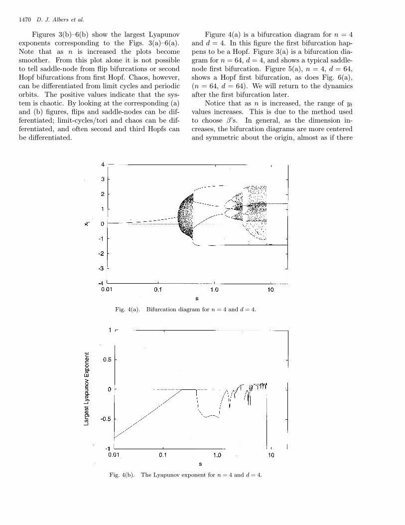
Figures 3(a)–6(a) are bifurcation diagrams forvarious n and d. In these figures the first 120 000 ytvalues are discarded and the next 128 are plotted.Each is a typical bifurcation diagram for its givenparameter values. Note that the meaning of typi-cal or characteristic for one set of n and d values isdifferent from that of another set of n and d values.There is more apparent variability in the dynamicsat low d than at high d. At high d most of the dia-grams look alike. At low d the diagrams are erraticbut differ in detail.


Figures 3(b)–6(b) show the largest Lyapunovexponents corresponding to the Figs. 3(a)–6(a).Note that as n is increased the plots becomesmoother. From this plot alone it is not possibleto tell saddle-node from flip bifurcations or secondHopf bifurcations from first Hopf. Chaos, however,can be differentiated from limit cycles and periodicorbits. The positive values indicate that the sys-tem is chaotic. By looking at the corresponding (a)and (b) figures, flips and saddle-nodes can be dif-ferentiated; limit-cycles/tori and chaos can be dif-ferentiated, and often second and third Hopfs canbe differentiated.

Figure 4(a) is a bifurcation diagram for n = 4and d = 4. In this figure the first bifurcation hap-pens to be a Hopf. Figure 3(a) is a bifurcation dia-gram for n = 64, d = 4, and shows a typical saddle-node first bifurcation. Figure 5(a), n = 4, d = 64,shows a Hopf first bifurcation, as does Fig. 6(a),(n = 64, d = 64). We will return to the dynamicsafter the first bifurcation later.

Notice that as n is increased, the range of ytvalues increases. This is due to the method usedto choose β’s. In general, as the dimension in-creases, the bifurcation diagrams are more centeredand symmetric about the origin, almost as if there


Fig. 4(b). The Lyapunov exponent for n = 4 and d = 4.



Fig. 5(b). Lyapunov exponent for n = 4 and d = 64.

were no bias term. This is because, as the numberof wij ’s is increased, the importance of the individ-ual wij is decreased, thus the importance of eachbias term is decreased. This does not affect the re-sults since there is no dynamical difference betweennetworks with and without bias terms (as stated inprevious sections).

4.4.1. A theoretical argument forthe first bifurcation

For random complex matrices, Girko [1983] proveda circular law which states that as the dimensionof a matrix becomes large, the probability of en-

countering any real eigenvalues is zero. Given arandom matrix, the eigenvalues will be uniformlydistributed within the unit circle. Making the un-wrought assumption that the set of Jacobians of oursystems are the same as a random sample of Girko’srandom matrices, we will put forth the following ar-gument. The set of eigenvalues lying on any partic-ular axis is of measure zero, thus the probability ofan eigenvalue being real is zero. Also, it would seemthat there is no difference between negative and pos-itive, thus no reason to favor a positive versus a neg-ative largest eigenvalue. Therefore, we should seeas many saddle-node bifurcations as flips. At lowdimensions we should see a much higher percentage



Fig. 6(b). Lyapunov exponent for n = 64 and d = 64.

of flips and saddle-node bifurcations because Hopfbifurcations need an even number of roots with noreal eigenvalues since they occur in pairs. At low di-mensions, arranging the roots such that they occurfrequently in even numbers, which is necessary forcomplex solutions, is not as probable as at higherdimensions. We briefly examined this numericallyfor random Girko-like real matrices. As the dimen-sion is increased the percentage of Hopf bifurcationsgoes from 0 to about 90 percent for a dimension of64. Given the aforementioned assumption, it wouldbe reasonable to assume that we would get approxi-mately the same distribution. Note that since com-plex eigenvalues occur in complex conjugate pairs,

given an odd dimension, at least one of the rootsmust be real.

4.4.2. Numerical results

Figure 7 shows the percentage of each bifurcation asthe dimension is increased for an intermediate num-ber of neurons. Much like the prediction above, theHopf’s start at about 40 percent of the first bifur-cations at d = 2 and increase to almost unity atlarge d. Also, notice that the percentage of flipsand saddle-nodes is, on average, equal throughoutthe range.

Unlike the random matrix case, we also have todeal with the n parameter. Figures 8 and 9 show


Fig. 7. Percent first bifurcation for n = 16, error bars represent the error in the probability.


the percentage of first bifurcation over an increasingrange of d at low and high n (n = 4 and n = 256).Note at high-n and low-d, the percentage of eachbifurcation is nearly equal. For the low-n, low-dcases, the percent of each bifurcation is not nearlyas close as at high-n. As d is increased, the percent-age of Hopf bifurcations rapidly increases so that, atd = 8, the percentages of each bifurcation is aboutequal to those of all n.

The n dependence is an artifact of how wechoose the β matrix. Consider a two-dimensionalsystem. For a Hopf bifurcation to occur, the dis-criminant must be negative. As we increase n, weare increasing the variance of the coefficients of the

matrix, thus pushing the expected value of the dis-criminant positive. The result is a decrease in Hopfbifurcations as n is increased at low d. As d isincreased this effect is washed out. ContrastingFigs. 7 and 8 you will notice that at d = 2 thepercentages of first bifurcations are quite different,but for d ≥ 8, Figs. 7 and 8 are almost identical.

In the high-d limit, we found that the Hopf bi-furcation was overwhelmingly dominant. We lookedat cases with d as high as 1024 and found the per-cent of first Hopf bifurcations approached unity.This confirms the result in [Doyon et al., 1993], thatin the limit of high d, the first bifurcation will beHopf.



4.5. Dynamics afterthe first bifurcation

Quantitative results for the probability of a givenbifurcation after the first requires developing theQ.R. algorithm [Eckmann & Ruelle, 1985] to allowthe tracking of quasiperiodic orbits. Tracking non-periodic orbits involves multiplying the Jacobiansat each time step and renormalizing to calculatethe eigenvalues. The numerical stability of spe-cific eigenvalues is not good when the number oftime steps is large. Although the stability of themodulus of the largest eigenvalue is acceptable andwould probably allow us to know when the systembifurcated, which eigenvalue crossed the unit cir-cle would not be certain. For this reason we willnow present qualitative trends that occur in thesesystems after the first bifurcation as gauged byobserving the largest Lyapunov exponent, period,correlation dimension, and bifurcation diagrams ofhundreds of systems.

4.5.1. A conjecture forthe second bifurcation

Doyon et al. [1993] proved a corollary of Girko’stheorem showing that the quasiperiodic route woulddominate when the dimension was high for theirmaps. For our purposes, we will first argue forflows and then adapt portions for maps. Considera flow on U that has undergone a Hopf bifurca-tion and is now living on a limit cycle. Now takea local cross-section V which is everywhere trans-verse to the flow. Next induce a discrete-time map

P : U → V thus creating the “first” return map.P is defined for a q ∈ U such that P (q) = ht(q)where t is the time required for the orbit to returnto V . This mapping has a fixed point which is thepoint q on the limit cycle. Considering the mappingP , increase the bifurcation parameter of the originalflow and keep track of the eigenvalues of the Jaco-bian of the discrete map. This will, on average, de-scribe which bifurcation will occur. Apply Girko’scircular law to the Jacobian of this map as we didfor the first bifurcation argument. For higher di-mensions, consider a flow with dimension d. Insteadof taking a 1-D “line transverse”, cut the flow witha hyper-surface (which will have dimension d − 1)that is everywhere transverse to the flow. Map thehyper-surface to itself. As above, increase the bifur-cation parameter and look at the eigenvalues of theJacobian of the map. As d goes to infinity, apply thecircular law; most of the eigenvalues lie on the unitdisk. The set of real eigenvalues is a set of measurezero with respect to the limiting Girko distribution.Because the set of real eigenvalues has measure zero,the second bifurcation must be Hopf. This sug-gests that as the dimension is increased, the pre-dominant route to chaos will be the quasiperiodicroute.

The argument for maps is somewhat differentbecause taking a Poincare section for a map is moredifficult. First consider the Jacobian at each timestep as given by the aforementioned matrix A. Sincethe probability that ai = 0, and thus the proba-bility that ad is zero, the A matrix will have fullrank. If At has full rank ∀t, then none of the A


matrices have eigenvalues that are equal to zero.Since

det(∏

At) = det(A1) det(A2) · · · det(At) (17)

and det(At) 6= 0 ∀t; det(∏At) 6= 0, and thus

∏At

is nonsingular. From here we only need to apply thecircular law to the

∏At to see that the quasiperi-

odic route will be dominant at high-d. Making theoriginal assumption rigorous is beyond the scope ofthis paper [Brock, 1997].

4.5.2. Between the first bifurcation and chaos

As stated above, the dynamics change consider-ably with d but not with n. The effect of n, forall d considered, is just to “smooth” the dynam-ics. The Lyapunov exponents are much more steadyand smooth, and the bifurcations are much moreapparent. Figures 3(b)–6(b) show typical largestLyapunov exponents over a range of s. Note thatthe dynamic transitions in Fig. 5(b) at low-n aremuch more “rough” than the changes in Fig. 6(b)at high-n. The largest Lyapunov exponent does notjump between positive and negative nearly as much.This behavior is typical over the range of n that westudied. However, n does not decrease the dynamicdiversity (types of transitions and bifurcations) ofa given network. Figures 3(a) and 4(a) show manyof the same phenomena and diversity even thoughthe number of neurons in Fig. 3(a) is much greaterthan in Fig. 4(a).

At d = 4 about 40 percent of the first bifur-cations are Hopf. After an initial Hopf bifurca-tion, recognizing a second Hopf is quite difficult,and they do not seem very frequent. More oftenthe second bifurcation appears to be a blue sky, outof a quasiperiodic orbit and into a periodic orbit.After this blue sky bifurcation the system eitherHopfs again, or period doubles to chaos [Fig. 4(a)],or just becomes chaotic [Fig. 3(a)]. Occasionally thesystem will oscillate between a quasiperiodic and aperiodic orbit several times before finally reachingthe chaotic region, but this usually occurs only forlow n. The other 60 percent of the bifurcationsare either flips or saddle-nodes. The only differ-ence between the dynamics after a saddle-node andafter a flip is that the saddle-node sometimes willjump from one branch of the fork to the other, pre-sumably because the initial conditions lie close to abasin boundary. Most often, after the flip or saddle-node, the system’s next bifurcation is a Hopf. Wedid see period-doubling cascades, but they were in-frequent prior to the onset of chaos except at low d.

Increasing n increases the probability and strength(magnitude of Lyapunov exponent) of chaos in thesystem.

The effect of d on the system dynamics is quitesignificant. As d is increased, the dynamic di-versity is greatly reduced. Networks with high dtend to be quite symmetric about the origin; thisis just an artifact of our method of choosing thew matrix. The most notable effect of increas-ing d is the increase of chaos for a given system.Flip and saddle-node bifurcations are almost neverseen in high-dimensional networks. Also, once thesystem has become chaotic, it very rarely showsperiodic windows until the s parameter is highenough to saturate the squashing function. In high-d systems, increasing n increases the range of thefunction. Doyon et al. [1993] conclude that forhigh-dimensional networks the second bifurcation isHopf. We also see this when the dimension is high,but discerning chaos from limit cycles and tori isoften difficult from the bifurcation diagrams. TheLyapunov exponent gives no insight if the secondbifurcation is Hopf, but at the onset of chaos, itbecomes positive. Doyon et al. [1993] also statethe quasiperiodic route to chaos dominates at highd. Our results agree, but speculating on how manybifurcations occur up to chaos is difficult.

4.6. The chaotic region

4.6.1. Bifurcation into chaos

The largest Lyapunov exponent for a nonchaoticmap equals the logarithm of the modulus of thelargest eigenvalue

λLyap = log |λeigen| (18)

For systems that follow the quasiperiodic route tochaos as previously stated, it is very difficult totrack specific eigenvalues, making it difficult to dis-cern which bifurcations occur into chaos. For thesame reason that it is difficult to calculate specificeigenvalues for limit cycles, it is difficult to trackthe eigenvalues in the chaotic region. We do trackthe modulus of the largest eigenvalue numerically(the Lyapunov exponent), which is used to distin-guish chaos from limit cycles. In systems followingperiodic routes, calculating the eigenvalues is dif-ficult. What is normally seen when plotting themodulus of the largest eigenvalue before and aftera flip or saddle-node bifurcation is quite expected.


At the bifurcation point, the modulus of the largesteigenvalue spikes up to one, and then just as quicklydrops back down. The largest Lyapunov exponent’sbehavior coincides with this behavior. What hap-pens at the bifurcation into chaos is not surprisingeither. The modulus of the largest eigenvalue spikesto one, the largest Lyapunov exponent spikes tozero, and it then proceeds to rise above zero. Atthis point we can no longer calculate the largesteigenvalue (or any eigenvalues) in a theoretic sense,but we continue to track the Lyapunov exponentnumerically. The modulus of the largest eigenvalueis greater than one.

4.6.2. Dynamics in the chaotic region

The chaotic region shows the least apparent dy-namic variability of any region. For the most part,the return maps of the chaotic regions all look verysimilar. (Much of this could of course be due tothat fact that we are projecting many dimensionson a plane.) As previously discussed, when n is in-creased, the range of the yt values increases, (due tothe β scaling) but that is the extent of the apparentvariability.

At low d the chaotic region is highly nonuni-form. The chaotic region contains windows of:Period-doubling sequences, limit cycles, low-periodorbits bifurcating to Hopf and then back into chaos;basically every type of dynamics imaginable. Aspreviously stated, Figs. 3(a) and 4(a) are typicalof the dynamic diversity at low d. Figures 5(a)and 6(a) are very different. Once the chaotic re-gion is reached, the system remains chaotic untilit is forced to be periodic by the saturation of thesquashing function. Figure 5(a) is an example ofwhat we call point-intermittent chaos. The chaoticregion is strongly dominated by a period-8 cyclewith chaos. The chaotic region in Fig. 5(a) is theregion corresponding to the positive Lyapunov ex-ponent region in Fig. 5(b). Figure 6(a) has a muchstronger chaotic region than Fig. 5(a), suggestingthat increasing the available complexity (increasein n), increases the chaos. Figure 6(a) is typical ofhigh d dynamics, limit cycles leading into a highlychaotic region.

4.6.3. Point-intermittent chaos

The chaotic region in Fig. 5 is especially interest-ing. When the network corresponding to Fig. 5 is

saturated, i.e.

tanh

sωi0 + sd∑j=1

ωijyt−j

= ±1 ∀i, j (19)

then there are eight possible states per dimension.2

(The upper bound on the period is then d2n.) Thesystem is chaotic when the squashing function isnot quite saturated. For most of the trajectorythe squashing function is saturated and the trajec-tory tends toward one of the eight attracting points.Certain combinations of inputs cause a neuron tobecome unsaturated, causing a point that missesthe attracting set by a significant amount caus-ing a positive largest Lyapunov exponent at thattime step. This miss effectively resets the peri-odic orbit; it also adds a nonattracting point tothe y array. A periodic orbit is interrupted be-fore it has completed one period by an intermit-tent point that is not one of the attracting points.After this miss occurs, the time-series resumes andagain consists of points in the attracting set. Ifthe system misses the attracting set enough times,the largest Lyapunov exponent will become posi-tive on average. The average time between missesis proportional to s. This behavior creates a se-quence of periodic trajectories that are strung to-gether by these points that miss the periodic orbit.The system is locally (over a short, periodic region)not chaotic, but, because of the averaging, globallychaotic.

The focus now is the cause of missing the peri-odic points. Computers have round-off errors whichcan play a significant role in the dynamics; we ar-gue that the chaos in Fig. 5 not such an artifact.Consider a function

ψ =

{±1 for |x| > a

tanh(x) for |x| ≤ a(20)

When all |x| > a the system is finite state andperiodic. When |x| is not greater than a for allx, then there are an infinite number of states thatoccur along with the eight attracting points. Ev-ery missed point not only “resets” the period, butsince it adds a new point into the yt array, allowsfor the possibility of saturating ψ in a different waythan the 8 attracting points could. The existenceof these intermittent points giving rise to other,

2There happen to be eight states for this system; there is a possibility of 2n states. We will discuss this in a later section.


different intermittent points, allows for an infi-nite number of possible intermittent points. As sis increased, the probability that ψ will be satu-rated increases, thus giving rise to less intermittentpoints.

4.7. Dynamics after the chaotic region

The dynamics after the chaotic region (large s) arequite interesting and surprising. At low d (Figs. 3and 4), there is a rapid (i.e. one or two incrementsof s), transition from chaos to periodicity. At low d,increasing n increases the complexity, as can be seenby comparing Figs. 3 and 4; high n tends to have agreater chance of chaotic windows after the periodicbehavior starts, but the dynamics are qualitativelythe same.

As before, at high d [Figs. 5(a) and 6(a)] thesituation is quite different. At low n the transitionfrom the chaotic to periodic region is quite difficultto find. Often there are strong periodic regions,with very small windows of high-period, quasiperi-odic, and chaotic orbits. If s is increased enough,the system becomes purely periodic. At high n thechaotic region occurs over a much larger range ofs. It is not until s is made very large (1000), thatthe periodicity becomes prominent. In this region,the transition between chaos and periodicity is verysimilar to that of the lower-n case, only much moregradual.

4.7.1. Theoretical argument forthe highest final period

As the s parameter is taken to infinity, for all practi-cal purposes (i.e. using a machine with limited pre-cision), the squashing function becomes a binary orstep function. This implies that the system mustrepeat, and thus cannot be chaotic. The dynamicsat high s consist of periodic orbits of varying pe-riod. There is often a dominant period, but even ats values as high as 1024 we see periodic windows.At high s, each neuron has two states, there are dsets of n neurons, and thus the highest period thenetworks can see is:

Ph = d2n (21)

We ran some experiments replacing the hyperbolictangent squashing function with a step function. Atvery low d we did see Eq. (21) reached. At d greaterthan 4 we never observed periods as high as Eq. (21)(c.f. [Kauffman, 1993]).

4.8. Interpretation ofthe qualitative results

Since all our results after the first bifurcation arevery qualitative, we would like to give some generalinterpretations of the results. Increasing n as couldbe deduced from reading [Hornik et al. 1989, 1990],smoothes the dynamics. Increasing n also increasesthe available dynamics, thus increasing the com-plexity, which increases both the probability andstrength of chaos. Increasing n increases the abil-ity to approximate, thus more dynamics can be ac-counted for, and seen. The d parameter increasesthe embedding dimension of the network and in-creases the probability of chaos. Another effect ofincreasing d is the slowing of the dynamics. Thisdecreases the largest Lyapunov exponent and alsosmoothes the dynamics. At high d most of the sys-tems appear very similar, whereas for low d the dy-namics are quite diverse. Low-d networks are al-most exclusively nonchaotic. Since we looked onlyat cases we knew were chaotic, we sampled little ofthe low-d network space. Many low-d networks stayat fixed points throughout the range of s consideredand thus look quite similar. Thus the apparent di-versity of the low-d networks might be due to thefact that we are only sampling 4 to 10 percent ofthe low-d space.

5. Conclusion

The major results of this study are: (1) as the num-ber of degrees of freedom are increased, the proba-bility of chaos approaches unity given a system thatis sufficiently nonlinear, (2) as the dimension is in-creased, the most probable first bifurcation is Hopf;the probabilities of saddle-node and flip bifurcationsare equal, and (3) qualitatively the quasiperiodicroute to chaos is the most probable as the dimensionis increased. The generality of the results hinges onthe methods used to assign the weight matrices, butgiven the conditions above, the results are general.The source code and additional details can be foundat http://sprott.physics.wisc.edu/neural/.

Acknowledgments

We would like to thank William Brock, Ian Dob-son, and Cosma Shalizi for many helpful discus-sions. The authors would like to thank Derek


Wright of the U.W. Madison Computer ScienceCondor group for help collecting data. Much ofthe data was run via the Condor High-ThroughputComputing System; without this resource our datacollection would be far more sparse. Informationconcerning the use of Condor can be found athttp://www.cs.wisc.edu/condor/

ReferencesAlbers, D. J., Sprott, J. C. & Dechert, W. D. [1996]

“Dynamical behavior of artificial neural networks withrandom weights,” in Intelligent Engineering SystemsThrough Artificial Neural Networks, eds. Dagli, C. H.,Akay, M., Chen, C. L. P., Fernanndez, B. R. & Ghosh,J. (ASME, NY), pp. 17–22.

Bowen, R. [1978] On Axiom A Diffeomorphisms, CBMSRegional Conference Series in Mathematics (A.M.S.Publications, Providence).

Brock, W. [1997] Private communication.Doyon, B., Cessac, B., Quoy, M. & Samuelides, M. [1993]

“Control of the transition to chaos in neural networkswith random connectivity,” Int. J. Bifurcation andChaos 3, 279–291.

Eckmann, J. P. & Ruelle, D. [1985] “Ergodic theory ofchaos and strange attractors,” Rev. Mod. Phys. 57(3),617–656.

Girko, V. L. [1983] “Circular law,” Theor. Prob. Appl.29, 694–706.

Grebogi, C., Hammel, S., Yorke, J. & Sauer, T. [1990]“Shadowing of physical trajectories in chaotic dynam-ics: Containment and refinement,” Phys. Rev. Lett.65, 1527–1530.

Guckenheimer, J. & Holmes, P. [1983] Nonlinear Oscilla-tions, Dynamical Systems, and Bifurcations of VectorFields (Springer-Verlag, NY).

Hornik, K., Stinchocombe, M. & White, H. [1989] “Mul-tilayer feedforward networks are universal approxima-tors,” Neural Networks 2, 359–366.

Hornik, K., Stinchocombe, M. & White, H. [1990] “Uni-versal approximation of unknown mapping and itsderivatives using multilayer feedforward networks,”Neural Networks 3, 535–549.

Kaufman, S. [1993] The Origins of Order, Self-Organization and Selection in Evolution (Oxford Uni-versity Press, NY).

l’Ecuyer, P. [1988] “Efficient and portable combinedrandom number generators,” Commun. ACM 31,742–749.

Naimark, J. [1959] “On some cases of periodic motionsdepending on parameter,” Dokl. Akad. Nauk, 736–739.

Newhouse, S. E. [1980] “Lecture on dynamical systems,”Dyn. Syst. 8, 1–114.

Press, W. H., Flannery, B. P., Teukolsky, S. A. &Vetterling, W. T. [1992] Numerical Recipes in C(Cambridge University Press, Cambridge).

Reick, C. & Mosekilde, E. [1995] “Emergence ofquasiperiodicity in symmetrically coupled, identi-cal period-doubling systems,” Phys. Rev. E52,1418–1435.

Ruelle, D. [1989] Elements of Differentiable Dynamicsand Vector Fields (Academic Press).

Sacker, R. S. [1965] “On invariant surfaces and bifur-cations of periodic solutions of ordinary differentialequations,” Comm. Pure Appl. Math., 717–732.

Takens, F. [1980] “Detecting strange attractors in tur-bulence,” in Lecture Notes in Mathematics 898,eds. Rand, D. & Young, L. (Springer-Verlag, Berlin),pp. 366–381.

Wang, W. & Cerdeira, H. A. [1996] “Dynamical behaviorof the multiplicative diffusion coupled map lattices,”Chaos 6, 200–208.

Wolf, A., Swift, J. B., Swinney, H. L. & Vastano, J. A.[1984] “Determining Lyapunov exponents from a timeseries,” Physica D16, 285–317.

routes to chaos in neural networks with random weights

Documents