Roope Uusitalo

Essays in Economics of Education

Research ReportsKansantaloustieteen laitoksen tutkimuksia 79:1999

Dissertationes OeconomicaeISBN 951 – 45 – 8705 – 9 (PDF version)

Foreword

Education as a way of increasing human capital is considered to be a basic factor in

the growth process of the aggregate economy. The returns to investment into human

capital are thus an important issue to analyze. In his Ph.D thesis Mr. Roope Uusitalo

studies the effects of education on earnings in Finland. Using a unique individual

level data set for men that also includes ability measures and information on family

background and appropriate estimation techniques Uusitalo presents new estimates

for the return of education in Finland, which are much higher than suggested by

earlier studies. Uusitalo also takes a broader issue by trying to explain changes in

earnings distribution. He augments a well-known single-index model of skills with the

the supply of skills and is able to account for a substantial portion of change in

earnings inequality between groups over the 1980s by changes in the supply of skills.

This study is part of the research agenda carried out by the Research Unit on

Economic Structures and Growth (RUESG). The aim of RUESG is to conduct

theoretical and empirical research into important issues affecting the growth and

dynamics of the macroeconomy, the financial system, foreign trade and exchange

rates, as well as problems of taxation and econometrics.

RUESG was established in the beginning of 1995 as one of the national centers of

excellence selected by the Academy of Finland. It is funded jointly by the Academy

of Finland, the University of Helsinki and the Yrjö Jahnsson Foundation. This support

is gratefully acknowledged.

Helsinki 30.12. 1998

Seppo Honkapohja Erkki Koskela

Professor of Economics Professor of Economics

Co-Director Co-Director

Acknowledgments

There are two great parts in a research project. The first is getting all exited about new

ideas and the possibilities that a new approach would offer. The second is when the

paper is finally done and can be put aside. It is the part in the middle that I had

troubles with. Endless efforts trying to make sense of the data and writing the text

over and over. Therefore, having finished this thesis, I would like to especially thank

all those that helped me with this middle part.

This thesis was written while I worked at the Research Unit on Economic Structures

and Growth at the Department of Economics at University of Helsinki. I am most

grateful to my colleagues for many fruitful discussions and to the directors of the unit,

professors Seppo Honkapohja and Erkki Koskela, for their support. As a part of the

program I also got a chance to spend an academic year at Princeton University. I

would like to thank great economists and wonderful characters Alan Krueger, Orley

Ashenfelter, Henry Farber, David Card and Bo Honore for their insight and

suggestions that not only helped solving contemporary problems with this thesis, but

also taught me a lot about how economic research really should be done. At Princeton

I also wrote the third chapter of this thesis together with Karen Conneely.

There are several others that played an important role in this project. My interest in

the economics of education originates to the research that I did while working at the

Research Unit on Sociology of Education at the University of Turku, and to the

discussions with professors Matti Viren and Osmo Kivinen. Rita Asplund and Reija

Lilja examined an earlier version of the first essay and provided useful comments in

the early stages of this project. Niels Westergård-Nielsen invited me to spend a few

months at Center of Labour Market and Social Research at Århus, where I finished

the final chapters. Tor Eriksson, Axel Werwalz, Joop Hartog, Guido Imbens and

Gordon Dahl among many others have commented parts of the thesis. Markus Jäntti

and Per-Anders Edin examined the final manuscript and made several suggestions

that improved the thesis. Without the help from Juhani Sinivuo at Finnish Defense

Forces Education Development Center, I would have not had the data that are used in

three of the four essays. Several people at Statistics Finland helped making that data

useful and answered my strange questions.

The Academy of Finland, the Yrjö Jahnsson Foundation, ASLA-Fulbright, the

Finnish Work Environment Fund and the Nordic Research Academy provided

financial support at various stages of this project. This support is gratefully

acknowledged.

Finally, I would like to thank my friends and family and, especially, my wife Miia for

making the life worth living during these long years that I spent working on this

dissertation.

Helsinki, December 1998

Roope Uusitalo

Contents

Chapter 1 Introduction ______________________________________________________1References ______________________________________________________________________ 7

Chapter 2 Return to Education in Finland ______________________________________9Abstract ________________________________________________________________________ 9

2.1 Introduction__________________________________________________________________ 9

2.2 Data _______________________________________________________________________ 11

2.3 OLS estimation results: the effect of ability bias ___________________________________ 16

2.4 Effects of endogeneity of education______________________________________________ 20

2.5 Conclusion __________________________________________________________________ 31

References _____________________________________________________________________ 33

Chapter 3 Estimating heterogeneous treatment effects in the Becker schoolingmodel____________________________________________________________________35Abstract _______________________________________________________________________ 35

3.1 Introduction_________________________________________________________________ 35

3.2 Variable returns to schooling and related estimation problems_______________________ 38

3.3 Data _______________________________________________________________________ 443.3.1 Background_______________________________________________________________________ 443.3.2 Descriptive statistics ________________________________________________________________ 47

3.4 Instrumental Variables and Control Function Estimation___________________________ 503.4.1 Selection of Instruments _____________________________________________________________ 503.4.2 IV and Control Function Estimates of the Return to Schooling _______________________________ 533.4.3 Allowing the Returns to Schooling to Vary with Observable Characteristics ____________________ 56

3.5. Maximum likelihood estimation of the system ____________________________________ 61

3.4 Conclusion __________________________________________________________________ 67

References _____________________________________________________________________ 68

Chapter 4 Schooling choices and the return to skills ______________________________70Abstract _______________________________________________________________________ 70

4.1 The nature of the problem _____________________________________________________ 70

4.2 Econometric issues ___________________________________________________________ 734.2.1 Ordered generalized extreme value model _______________________________________________ 744.2.2 Selectivity correction _______________________________________________________________ 764.2.3 Calculating the opportunity costs ______________________________________________________ 79

4.3 Data _______________________________________________________________________ 80

4.4 Empirical results_____________________________________________________________ 844.4.1 Correlation structure in the test scores __________________________________________________ 844.4.2 Simple wage equations ______________________________________________________________ 864.4.3 Schooling choice___________________________________________________________________ 894.4.4 Selectivity corrected earnings equations_________________________________________________ 914.4.5 Counterfactual outcomes_____________________________________________________________ 92

5 Conclusion ___________________________________________________________________ 95

References _____________________________________________________________________ 96

Appendix. Description of the Finnish Army basic ability test ___________________________ 98Part 1, Basic skills (Peruskoe 1)____________________________________________________________ 98Part 2, Leadership inventory (Peruskoe 2)____________________________________________________ 98

Chapter 5 Trends in between- and within-group earnings inequality in Finland ______100Abstract ______________________________________________________________________ 100

5.1 Introduction________________________________________________________________ 100

5.2 Recent trends in the distribution of earnings in Finland ___________________________ 1035.2.1 Trends in aggregate time series_______________________________________________________ 1045.2.2 Evidence from microdata ___________________________________________________________ 112

5.3 Explanations for the observed changes__________________________________________ 1165.3.1 Single-skill model _________________________________________________________________ 1175.3.2 Application for cell means and quantiles _______________________________________________ 1195.3.3 The effect of supply changes_________________________________________________________ 120

5.4 Empirical results____________________________________________________________ 1225.4.1 Estimates of the single-skill model ____________________________________________________ 1245.4.2 Conjectures on the intervening mechanisms: Institutions do matter. __________________________ 130

5.5 Concluding comments _______________________________________________________ 133

References ____________________________________________________________________ 134

Appendix 1 Cross - section regressions_____________________________________________ 136

Chapter 1

Introduction

Some forty years after the birth of the human capital theory, education is still one of the

central topics in the public policy debate. This is particularly true in Finland which has one of

the most expensive education systems in the world. The need to decrease public spending

causes pressure to cut the resources that the society allocates to running the school system. On

the other hand, it is widely realized that an increasingly complex society and rapid technical

change requires highly educated workforce, if the country wishes to succeed in the

international competition. Interestingly enough, most of the arguments in this debate are cast

in economic terms.

The basic principle of the human capital theory that stresses the role of education as a

productivity enhancing investment (Becker 1964) is widely accepted in this discussion.

Education policy is directed to meet the skill needs of the modern workplace and to improve

the performance of the individuals in the labor market. In fact, education is seen almost as a

universal cure to some of the most severe economic problems such as unemployment and

poverty. Human capital is also a regarded as key factor in generating higher productivity and

economic growth (e.g. Barro and Sala-i-Martin, 1995).

This thesis focuses on the effect of education on individual earnings. This does not

necessarily fall far from measuring its effects on productivity. Only few datasets contain

better measures of the productivity of individuals. On the other hand, earnings differences are

an important outcome themselves. Developments in inequality and poverty have become

increasingly important topics and, after recent developments in US and UK, also attracted

more and more attention in academic research.

A central theme in this thesis is, how can causal inferences be drawn when only observational

data are available. In the natural sciences, causal relationships can be identified using

carefully designed controlled experiments. To a limited extent, this is also possible in the

social sciences, but education is far outside the scope for technically feasible and morally

acceptable experiments. The only option is to use experiments that are set up by nature.

2

Nature allocates people with different amounts of talent and opportunities. Nature has no

need to be fair. Using such natural experiments and economic theory, some inferences on the

causal relationships can be drawn.

The approach in this thesis is both structural and parametric. Economic theory is used to

formulate the models and, in some cases, to provide empirically testable hypotheses.

However, the emphasis is clearly on the empirical work. A lot of effort has been devoted to

stretching the statistical methods so that various parameters could be consistently estimated.

This thesis consists of four essays, one of which is joint work with Karen Conneely at

Princeton University. All the essays are written to be read by themselves. Therefore, some

degree of overlap and repetition is unavoidable. In the following, I briefly introduce the topics

of each and summarize their main findings.

Return to education in Finland

The first essay is a straightforward attempt to estimate the rate of return to the years of

education in Finland. The major issues are potential biases in the estimates caused by

measurement errors in education, ability bias and the endogeneity of educational choice.

These problems are tackled by controlling for individual ability differences using data from

the Finnish Army psychological tests, and by applying the instrumental variable method in the

estimation.

The approach in the first essay is in line with traditional mainstream empirical human capital

research. The central issues were discussed already by Griliches (1977). Willis (1985)

provides a survey of earlier studies and Card (1994) of more recent studies. Earlier studies

relied heavily on test scores in an attempt to remove ability bias from the return to schooling

estimates. Generally, it was found that failing to account for the (pre-school) ability

differences leads to an overestimate of the return to schooling. This conclusion was largely

refuted by a number of studies in the 1990's that relied on various natural experiments and

instrumental variable techniques. The instrumental variable estimates were systematically,

though often insignificantly, higher than comparable ordinary least squares estimates. Until

just a few years ago the empirical evidence was limited to the US data. During last few years

several studies have appeared in the UK (Harmon and Walker 1995; Dearden 1995), Sweden

(Meghir and Palme 1997), Australia (Miller, Mulvey and Martin 1995) and Netherlands

3

(Levin 1997). The results in these studies were quite similar to the US findings. This thesis

adds one more piece to this accumulating international evidence.

The empirical estimates show that, accounting for measurement error, endogeneity and ability

differences, the estimates for the return to additional years of schooling are between 11 and

13%. These are significantly higher figures than earlier estimates from Finnish data (e.g.

Asplund 1993). The chapter concludes that the positive ability bias in the ordinary least

squares estimates is more than offset by a negative bias caused by endogeneity or

measurement error.

Estimating heterogeneous treatment effects in the Becker schooling model1

The second and third essays are more focused on statistical issues. In the second essay we

take seriously the Becker schooling model, which states that people decide on the schooling

investments based on the marginal costs and marginal benefits of education. We note that if

the marginal returns vary across individuals, there is no single parameter for the return to

schooling. Instead, the appropriate model is a variant of a random coefficients model. The

estimation problem is further complicated by the correlation of this random coefficient and

the endogenous schooling variable. However, we show that the average return to schooling

can still be consistently estimated with traditional instrumental variable method. We also

provide maximum likelihood estimates on the extent of unobserved and observed variation in

the returns to schooling across individuals.

The implications of variation in program effects are dealt with in the recent ''treatment

effects'' literature. Angrist and Imbens (1995) demonstrate that the instrumental variable

method can be used to calculate average causal effects of the treatment. Imbens and Angrist

(1994) show that instrumental variables estimates identify ''local average treatment effects''.

Card (1994) discusses these issues less formally in the context of estimating returns to

schooling. Heckman (1995, 1997) shows that the conclusions on the consistency of

instrumental variables estimates are only valid if the program effects do not vary across

individuals or if the variation in program effects does not influence the program participation.

Heckman's arguments concern the effect of dichotomous treatment variable. In our essay we

show that in a continuous case discussed by Garen (1984) there are some restrictive, but not

1 Joint work with Karen Conneely

4

unreasonable assumptions, under which the instrumental variables estimates are still

consistent. As empirical evidence we compare instrumental variables estimates to the control

function estimates proposed by Heckman and note that the results are close to identical.

Schooling choices and return to skills

The third essay casts some of the issues treated in the first two essays in a discrete choice

framework. Eventual education level is determined by a sequence of discrete choices. This

essay is an attempt to model these choices and the implications of the choice mechanism on

the conditional earnings distributions in the different education levels. The choices among

several potentially correlated alternatives are modeled using an ordered generalized extreme

value model and predicted outcomes in different education levels are calculated. A dataset

that includes measures of various personality traits is used to examine whether rewards for

skills vary by the education level and whether this leads to the choices being determined

according to comparative advantage.

The econometric methodology in this essay is based on work on selectivity issues in the

polychotomous choice models by Lee (1982, 1983, 1995). The Lee approach has been

criticized for its restrictive assumptions on the correlation pattern of the unobservable

components (Small, 1987, 1994; Schmertmann, 1994; Vella and Gregory, 1996). In this essay

some of these assumptions are relaxed. However, it is shown that, a multinomial logit model

used by Lee is a reasonable approximation for the data generating process.

Another issue that has caused a major controversy in public press as well as in academic

community is the effect of cognitive skills on the success in later life. This debate started

from publication of ”The Bell Curve” by Herrnstein and Murray (1994). Though the

methodology and the conclusions of the book have been strongly rejected by later research,

the debate has launched what could be called a new research program (e.g. Ashenfelter and

Rouse 1995; Cawley, Heckman and Lytchacil, 1998). Most of this research avoids biological

arguments on heriditance of personality traits but concentrates on the labor market effects of

some measurable skills. Understandably, useful data are hard to find and most of the existing

research in the U.S. utilizes cognitive skill measures available in National Longitudinal

Survey of Youth. My essay provides more empirical evidence to this discussion by using a

wide range of personality test scores that were available in the Finnish Army databases. In

5

addition, the essay takes the discussion on the effects of cognitive skills back to the context of

the original Roy model (Roy 1951) where individuals choose their careers based on their skill

endowments and the returns to these skills in the different sectors.

The empirical results show that several dimensions of skill have significant effects on

schooling choices and earnings. However, the effects on earnings are quantitatively small;

even detailed information on ability and personality factors explains only a small fraction of

earnings variation at a given level of schooling.

Trends in between- and within-group earnings inequality in Finland

The fourth essay deals with the changes in earnings inequality. Inequality has become a very

active research area during the 1990's. The increase in research activity has largely been the

economic profession's response to the increase in earnings differences in the U.S. over the

1980's. This observation required an explanation. Some of the most successful explanations

argued in terms of changes in unionization, opening of international trade, changes in the

supply of skilled labor, and the requirements of advanced technology (Levy and Murnane

1992). Of these, only the technology explanation seems to fit the facts. Changes in the

technology in the 1980’s appear to have been skill-biased, favoring workers who posses

resources and skills to take an advantage of the technological developments.

This essay focuses on one of the more difficult puzzles of the development. A large fraction

of the change in the earnings dispersion has occurred between observationally identical

workers. A starting point for the explanation is the single-skill model (Card and Lemieux,

1996). In the single-skill model a fraction of the dispersion of earnings within a group of

workers with similar education and experience is caused by unobserved differences in ability.

A technological change that favors the high-ability workers is then expected to increase the

productivity differences both between workers in the different skill groups and increase the

dispersion within each group. In the essay, I extend the single-skill model by introducing

imperfect substitutability between workers in different skill groups. This creates a role for

changes in the relative supply of workers. With this simple extension, the changes in

inequality can be analyzed in a familiar supply-demand framework.

Empirical evidence suggests that this extension aids understanding the changes that occurred

in the Finnish income distribution over the 1980's. The rapidly increasing supply of educated

6

workers seems to have prevented the increase in earnings inequality that occurred in several

other countries. On the other hand, the model does not fully explain the changes in the within-

group distribution. The paper provides some evidence that changes in institutional setting, in

particular changes in the degree of centralization in wage bargaining, may be responsible for

these changes.

Data for the three first essays are created by merging information from the databases of the

Finish Army with longitudinal census data. The sample for the first essay is drawn from the

men who were in the army in 1970. The second and third essay use a much larger sample of

men who were performing their military service in 1982. The army performs various ability

and personality tests for all recruits. Since military service is compulsory test scores are

available for the majority of the male population. Therefore, labor market effects of

individual characteristics can be analyzed using much larger samples than in previous studies.

The army data is then matched with census files using social security numbers that were

available in conscription records. Merging data from the army sample required a dataset that

contained the whole population. The census data was the only possibility and, although

lacking some desirable information, the data were sufficiently rich for the analyses performed.

In addition to a large sample size, the Finnish census data have several appealing features.

Since most information is based on registers and direct reports from, for example, tax

authorities, data is free from recall errors that are common in survey data. Reliability of not

only earnings, but also, for example, schooling information is likely to be higher than in most

commonly used datasets. Also attrition from the sample is very small.

The fourth essay utilizes microdata from the Income Distribution Surveys (IDS). Designed for

this purpose, the IDS data are the best available source for income distribution studies. IDS

contains a random representative sample from the population. Although the main income

concept is disposable income of the household, detailed information on the market income of

individuals is also available. These data also contain information on an important group for

which data were not available in army databases, namely the women.

7

References

Angrist, J. and G. Imbens (1995) ''Two-Stage Least Squares Estimation of Average Causal Effect in

the Models with Variable Treatment Intensity'', Journal of American Statistical Association 90, 431-

442.

Ashenfelter, O. and C. Rouse (1995) ”Cracks in the Bell Curve: Schooling Intelligence and Income in

America”, Unpublished paper, April 1995.

Asplund, R. (1993) ”Essays on Human Capital and Earnings in Finland”, The Research Institute of

the Finnish Economy, Series A18.

Barro, R. and X. Sala-i-Martin (1995) ”Economic Growth”, New York: McGraw-Hill.

Becker, G. (1964) ”Human Capital. A Theoretical and Empirical Analysis with a Special Reference

to Education”, New York: Cambridge University Press.

Card, D. (1994) ''Earnings Schooling and Ability Revisited'', NBER Working Papers 4832.

Card, D. and T. Lemieux (1996) ''Wage Dispersion, Returns to Skill, and Black-White Wage

Differentials'', Journal of Econometrics 74, 319-361.

Cawley, J., J. Heckman and E. Vytlacil (1998) ''Meritocracy in America: Wages within and Across

Occupations'', NBER Working Papers, 6646.

Dearden, L. (1995) “The Returns to Education and Training for the United Kingdom'', Unpublished

Ph.D. Dissertation, University College London.

Garen, J. (1984) ''The Returns to Schooling: A Selectivity Bias Approach with a Continuous Choice

Variable'', Econometrica 52, 1199-1218.

Griliches, Z. (1977) ''Estimating Returns to Schooling: Some Econometric Problems'', Econometrica

45, 1-22.

Harmon, C. and I. Walker (1995) ''Estimates of the Economic Return to Schooling for the UK'',

American Economic Review 85, 1278-1286.

Heckman, J. (1995) ''Instrumental Variables: A Cautionary Tale'' NBER Technical Working Papers

185.

Heckman, J. (1997) ''Instrumental Variables: A Study of Implicit Behavioral Asumptions Used in

Making Program Evaluations'', Journal of Human Resources 32, 441-461.

Herrnstein, R. and C. Murray (1994) ''The Bell Curve'', New York: Free Press.

8

Imbens, G. and J. Angrist (1994) ''Identification and Estimation of Local Average Treatment Effects'',

Econometrica 62, 467-476.

Lee, L. F. (1982) ''Some Approaches to the Correction of the Selectivity Bias'', Review of Economic

Studies 49, 355-372.

Lee, L. F (1983) ''Generalized Economic Models with Selectivity'', Econometrica 51, 507-512.

Lee, L. F. (1995) ''The Computation of Opportunity Costs in Polychotomous Choice Models with

Selectivity'', The Review of Economics and Statistics, 423-435.

Levin, J. (1997) ''Instrumental Variables Technique and the Rate of Return to Ecucation for Dutch

Males'', Unpublished manuscript.

Levy, F. and R. Murnane (1992) ''U.S. Earnings Levels and Earnings Inequality: A Review of Recent

Trends and Proposed Explanations'', Journal of Economic Literature 30, 1333-1381.

Meghir, C. and M. Palme (1997) ''Assessing the Rate of Returns to Education Using the Swedish

1950 Education Reform'', Unpublished manuscript.

Miller, P., C. Mulvey and N. Martin (1995) ''What Do Twins Studies Reveal About the Economic

Returns to Education? A Comparison of Australian and U.S. Findings'', American Economic Review

85, 586-599.

Roy, A. (1951) ''Some Thoughts on the Distribution of Earnings'', Oxford Economic Papers 3, 135-

146.

Schmertmann, C. (1994) ''Selectivity Bias Correction Methods in Polychotomous Sample Selection

Models'', Journal of Econometrics 60, 101-132.

Small, K. (1987) '' A Discrete Choice Model for Ordered Alternatives'', Econometrica 55, 409-424.

Small, K. (1994) ''Approximate Generalized Extreme Value Models of Discrete Choice'', Journal of

Econometrics 62, 351-382.

Vella, F. and R. Gregory (1996) ''Selection Bias and Human Capital Investment: Estimating the Rates

of Return to Education for Young Males'', Labour Economics 3, 197-219.

Willis, R. (1986) ''Wage Determinants: A Survey and Reintepretation of Human Capital Earnings

Functions'', Chapt. 10 in O. Ashenfelter and R. Layard eds.: Handbook of Labor Economics, Volume

I, Elsevier, 525 - 602.

9

Chapter 2

Return to Education in Finland1

Abstract

This study presents estimates of the return to education in Finland using anindividual-level data set that also includes ability measures and information on familybackground.

It is found that ability test scores have a strong effect on the choice of education andon subsequent earnings. Estimating the return to education with no information onability leads to an upward bias in the estimates. However, this bias is more than offsetby a downward bias caused by endogeneity or measurement error. Instrumentalvariables estimates that utilize family background variables as instruments produceestimates of the return to schooling that are approximately 60% higher than the leastsquares estimates.

Keywords: return to education, ability bias, selectivity.

JEL Classification: J24.

2.1 Introduction

In this paper I report evidence on the returns to schooling that exploits a unique data set

containing ability test scores from the Finnish army. Since military service is compulsory in

Finland and all the men are tested at the beginning of their service, it is possible to construct a

linked data set that includes test scores from military service records, income data from tax

authorities and information on schooling and family background from Finnish Census. Using

these data, I estimate returns to schooling in Finland using test scores as independent

variables and using family background as an instrumental variable to correct for measurement

error and / or endogeneity in school choices.

1 A shorter version of this chapter is forthcoming in Labour Economics

10

Despite a long debate in the empirical literature on earnings determination, a consensus on the

direction and size of the bias in the simple ordinary least squares (OLS) estimates of returns

to schooling has yet to appear. Ability differences between individuals with differing amounts

of education may bias estimates upward. Alternatively, a number of recent studies suggest

that the OLS estimates are more likely to be biased downward. Resolving this issue

conclusively would require a series of controlled experiments with random assignments of

educational levels.

The majority of the earlier literature on the return to schooling was concerned with the

potential omitted variable bias caused by the correlation of unobserved individual abilities

with both schooling and earnings. The simplest way to correct for this ability bias appeared to

be to obtain a good measure of ability and to include it in the estimated earnings function.

Typically, the data sets used for studying the effect of ability bias were constructed using

samples that included data on various ability tests taken during military service (Taubman and

Wales, 1973). More recent evidence is almost entirely based on a few large scale longitudinal

surveys, especially the National Longitudinal Survey of Youth (NLSY), initially surveyed in

1979 (e.g. Blackburn and Neumark 1993, 1995). Including ability measures in earnings

equations decreases the schooling coefficients in all these studies.

Other recent approaches for correcting potential biases in the return to education estimates

include estimating earnings functions from differences within twins or siblings (Ashenfelter

and Krueger 1994; Miller, Mulvey and Martin 1995) and resorting to various “natural

experiments” that exploit exogenous sources of variation in schooling (Angrist and Krueger

1991, 1992; Card 1993; Butcher and Case 1994; Harmon and Walker 1995). All these studies

conclude that the OLS estimates of the return to education are likely to be biased downward.

Corrected estimates range from only slightly above OLS estimates (Angrist and Krueger

1991, 1992) to more than double the OLS estimates. (Harmon and Walker 1995). It is

apparent that the two different approaches used in the literature lead to different conclusions.

In this paper I follow the tradition in Griliches (1977) and include various ability measures in

earnings equations, but I also treat education as endogenously determined or measured with

error, and use information on family background as instrumental variables for education.

Thus, I take advantage of the available information on ability of a large sample as in earlier

11

literature, but I also follow the more recent literature in attempting to provide a credible

estimate of tha causal effect of schooling on earnings.

My analysis is based on a randomly selected sample of 2,000 men who took the Finnish army

ability test in 1970. By combining army test scores, administrative records and a longitudinal

data set from Finnish population censuses, I constructed a new panel data set that includes

ability measures and information on education and earnings as well as other control variables.

Compared to commonly used large scale survey data sets such as the NLSY, constructing the

new data set was very inexpensive. Despite its low cost, the data contain comparable

measures of cognitive ability, together with information on schooling and earnings. Since this

information is based on administrative records from schools and tax authorities, it is likely to

be at least as reliable as self-reported information. The Finnish longitudinal census data file

contains information collected every five years (1970, -75, -80, -85 and -90), and it covers a

longer time span than, for example, the NLSY. It seems likely that the data construction

methods used in this paper may well be applicable also in other countries where schooling

and military records may easily be linked together.

The data used in this paper is described in section 2.2. Section 2.3 presents the basic ordinary

least squares estimates after controlling for measured ability differences. In section 2.4 the

differences in family background are used as an exogenous source of variation in education to

create instruments for schooling and to provide estimates free of measurement error /

endogeneity bias. Section 2.5 summarizes with a short discussion of why IV and OLS

estimates differ.

2.2 Data

The ability test scores used in this study were obtained from the Finnish Defense Forces Basic

Ability Test (Peruskoe 1) developed by the Finnish Defense Forces Education Development

Center. The test has been administered in unchanged format from 1955 to 1980 for all new

recruits at the beginning of their service. In 1981 the ability test was revised and

12

complemented with a broader personality test. Only the ability test is used here. Since military

service is compulsory in Finland, the tested group contains almost the entire male cohort.2

The ability test consists of three subtests measuring verbal ability, analytical reasoning and

mathematical reasoning. Each subtest has 40 multiple choice questions that become gradually

more difficult. The measure of verbal ability consists of three types of questions: the

examinee has to choose which word is a synonym or antonym of a given word, choose which

word pair displays a similar relationship to a given word pair and choose which word does

not belong to a given group of words. In the analytical reasoning section, the test-taker is

given a matrix of figures arranged according to a certain rule, but with one figure missing.

The examinee has to decide which figure completes the matrix. Finally, the mathematical

reasoning section consists of simple arithmetic operations, short problems given in a verbal

form, and completing number series arranged according to a certain rule.

The scores from different parts are combined and scaled in a range from 1 to 9. This

combined score is used as a minimum qualification in the selection of the rookies that are

given officer training. Typically a minimum score requirement for selection to the

noncommissioned officers’ school (RAUK) is 4 and for selection to the reserve officers’

school (RUK) minimum is 6.

The selected sample consists of a random sample of 2,000 recruits3, who had taken the Basic

Ability Test in 1970, from the files of the Finnish Defense Forces Education Development

Center. Conscription records were then used to match the names to the social security

numbers. Finally, the sample was connected to a longitudinal data set of Finnish population

censuses.

2 A system where every applicant is accepted for alternative (nonmilitary) service was adopted in1987. Prior to that applications were examined by military authorities and the National ExaminationBoard. Less than 3% of the age group were exempted from military service due to religious or ethicalconviction. In addition, approximately 10% were disqualified for health reasons. (Scheinin 1987)3 The sample size was limited by the difficulty of collecting the ability test scores. The scores arestored on microfilm and had to be gathered manually. Further difficulties arose because in 1970, thearmy did not use social security numbers but only names (in some cases only last names and firstinitials). Since 1982, test scores are electronically stored in a database with proper identification. Infact, a larger sample of approximately 37,000 recruits from the year 1982 was also collected but isnot used in this study because of the short time span up to the final year of observation of 1990.

13

The census file contains information on all 6.4 million residents of Finland gathered at the

censuses of 1970, -75, -80, -85 and -90. Most importantly, for the purpose of this study, the

census file includes information on taxable earnings from the tax administration4 and detailed

information on completed degrees.

Schooling information in the census is based on the Register of Degrees and Examinations

compiled by Statistics Finland. The register was created in the 1970 census and supplemented

in 1980 with a questionnaire concerning degrees completed before 1970. The register is

updated yearly with the information submitted directly by educational institutions. The data

contains a five-digit code in which the first digit indicates the level of education. For most of

the analysis, degrees completed are converted to years of schooling according to the Standard

Classification of Education by Statistics Finland. Individuals who have not completed any

post-compulsory education are assigned compulsory nine years of schooling. For a part of the

analysis, a discrete grouping is also used classifying levels 1-2 as compulsory, level 3 as

vocational, levels 4 and 5 as upper vocational and levels 6 - 8 as university education.

In addition to the records for the recruits, the census data were used to find data on the

parents. Information concerning profession, income, education and socioeconomic status of

the parents was collected to analyze the effects of the family background. Information on

parents was collected from the earliest available census of 1970 so that measures of family

background refer to the period when the sample males were about 18 - 20 years of age.

The final data set is constructed by combining information from the census years 1975, -80, -

85 and -90. Observations are included from the years when individuals had reached their final

(1990) level of schooling and were working full-time5. For individuals who appear in more

than one census, all the variables are averaged over the years. Due to the inability to identify

all the individuals of the original sample from the census data and to missing information on

4 Statistics Finland customarily top codes the income information in census data so that the actualincomes of the highest 5% are replaced with the average income of that group. For this studyuncensored information was available5 Data on the months worked is rather unreliable in census. Information is based on a questionnaire.Respondents who did not answer the question on months worked in census were coded to haveworked for 0 months. Also, some respondents seem to have (incorrectly) subtracted vacation periodfrom the number of months worked (CSO 1991). Here only those with annual earnings of FIM 50,000in 1990 currency (approximately 80% of the lowest government salary) or more are considered to befull-time workers.

14

those who had migrated or died, only 1,537 men remain in the final data. Restricting the

analysis to those who had valid information on education and who were full-time workers in

at least one census year further reduced the sample size to 1427. Of these, family background

information was missing for 421 men so that only 1,016 observations could be used in the

analyses involving the effect of family background. Some descriptive statistics of the full-

time workers sample that was used in the final estimations are presented in Table 1.

15

Table 1 Descriptive statisticsall observations observations with

non-missing familybackground variables

mean standarddeviation

mean standarddeviation

Years of educationa 11.0 2.1 11.1 2.2Ed level 2 (compulsory, 9 years) 0.35 0.48 0.33 0.47Ed level 3 (appr. 10-11 years) 0.37 0.48 0.36 0.48Ed level 4 (appr. 12 years) 0.16 0.36 0.17 0.37Ed level 5 (appr. 13-14 years) 0.05 0.23 0.06 0.23Ed level 6 (appr. 15 years) 0.02 0.15 0.02 0.15Ed level 7 (appr. 16 years) 0.05 0.21 0.06 0.22Ed level 8 (more than 16 years) 0.01 0.08 0.01 0.08Earnings, FIMb 112 542 43 680 113 460 45 256Potential work experiencec 15.33 2.91 15.28 2.93Age 33.36 2.84 33.41 2.86Verbal test score 23.67 8.31 23.88 8.37Analytical test score 21.83 6.20 21.91 6.16Math test score 22.88 10.43 23.11 10.36Lived in Helsinki area 0.11 0.27 0.10 0.27Lived in other urban aread 0.46 0.44 0.44 0.44Works in the private sector 0.63 0.41 0.60 0.42Married 0.71 0.46 0.73 0.44Father’s taxable income in 1970 13 907 13 315Father upper white-collar 0.04 0.20Father lower white-collar 0.11 0.32Father’s education: vocational 0.07 0.25Father’s educ.: upper vocational 0.07 0.26Father’s educ.: university degree 0.03 0.17Father’s information missing 0.29 0.45 0.00 0.00Observed in 1975 0.69 0.46 0.68 0.47Observed in 1980 0.81 0.39 0.81 0.39Observed in 1985 0.86 0.35 0.86 0.35Observed in 1990 0.86 0.35 0.86 0.34N 1427 1016

All figures refer to averages over the years that an individual was a full-time worker in census.a The years of education variable was constructed from information on the highest degree achievedaccording to the standard educational classification of Statistics Finland.b Annual earned income from tax records. Includes wage and entrepreneurial income but excludescapital income. Converted with CPI to 1990 currency and averaged over years when an individual isobserved in census.c Age-years of schooling-7. Average over census years when an individual is observed.d A city where over 90% of inhabitants live in densely populated area.

16

2.3 OLS estimation results: the effect of ability bias

The earnings differences between groups with different educational levels reflect not only the

earnings effects of education but also the effects of the other characteristics of these groups.

Notably, it is likely that those with more and less education differ on the average level of

ability. Inferences on the effect of education based on the observed earnings differences may

well be biased because part of the variation in earnings is caused by the variation in ability.

To give an impression of the ability differences in the sample between individuals having

completed different levels of schooling, mean scores on the ability tests by the level of

education are reported in Table 2. It appears that mean scores on all the ability tests vary

systematically with the level of education. The differences are rather large: for example, the

average math test score of university graduates is almost double the average score of those

who have completed only the compulsory nine years of schooling.

Table 2 Mean ability test scores according to the level of educationN math test verbal test analytical test

Compulsory education(level 2)

495 17.6(0.43)

20.0(0.32)

19.2(0.25)

Vocational education(level 3)

524 21.0(0.41)

21.6(0.32)

20.8(0.25)

Upper vocational educ.(levels 4 – 5)

301 31.0(0.40)

30.0(0.37)

25.9(0.28)

University education(levels 6 – 8)

107 33.4(0.48)

33.0(0.52)

27.6(0.42)

Standard errors of means in parentheses

Figure 1 illustrates the effect of ability on earnings with a simple plot. In figure 1, the sample

has been divided into four equal sized subgroups according to the percentile rank of the total

score in the ability test. Log average annual earnings in 1990 are calculated for these groups

at each schooling level and plotted against schooling. As can be seen in Figure 1, groups with

higher ability have higher average earnings in all schooling levels. The effect of ability is

rather similar in all levels of schooling. Also, average earnings increase more rapidly with the

length of schooling in the whole sample than within groups of approximately similar ability,

which indicates that the effect of schooling on earnings may be overstated if the ability

differences are not accounted for.

17

Figure 1 Log average annual earnings in 1990 according to the level of education withingroups of similar ability

compulsory (9 years)

vocational (11 years)

upper vocational(12-14 years)

university (16+ years)

11

11,2

11,4

11,6

11,8

12

12,2

12,4

log

annu

al in

com

e

compulsory (9 years)

vocational (11 years)

upper vocational(12-14 years)

university (16+ years)

0 - 25 %26 - 50 %51 - 75 %76 - 100 %

In this study the abilty test scores are utilized to control for the effects of ability. In the basic

specification log annual earnings6 of full-time workers are regressed on a set of schooling

variables and ability test scores. In all equations the dependent variable and the time-variant

independent variables are averages over the years that the individual was included in the

sample. The equations also include controls for (potential) work experience and dummies for

region and sector, as well as a set of dummies indicating if an individual was missing from

any census year.

The ordinary least squares estimation results presented in Table 3, column (1) indicate that

the returns to education are approximately 9.3%7 when ability differences are not controlled

for. This estimate is well in line with earlier studies using Finnish data (Asplund, 1993). The

other estimated coefficients also seem reasonable. The experience profile is concave with a

one-year difference in work experience increasing earnings by 5% for the first year.

Compared to rural areas, earnings are 11.2% higher in the capital area and 5.3% higher in

other urban areas. Private sector earnings are approximately 3.3% higher than earnings in the

public sector.

6 Annual earnings are preferred to monthly earnings because the measurement and coding errors inmonths worked would cause an error in monthly earnings7 The percentage differences reported in text are calculated from the antilog of parameter estimates(eb-1)*100, where b is the estimated schooling coefficient in the log earnings equation. For small bthe estimated parameters of the log earnings equation are approximately equal to the proportionaldifference.

18

Table 3 OLS regression results. Dependent variable is log annual earnings.No test scores Test scores included

(1) (2) (3) (4)Intercept 10.18 11.04 10.26 10.92Years of education 0.089

(0.006)0.074

(0.006)Ed level 3a 0.018

(0.017)0.004

(0.017)Ed level 4 a 0.239

(0.025)0.189

(0.027)Ed level 5 a 0.352

(0.039)0.287

(0.040)Ed level 6 a 0.458

(0.043)0.396

(0.045)Ed level 7 a 0.767

(0.053)0.701

(0.054)Ed level 8 a 0.737

(0.100)0.668

(0.101)Experience 0.049

(0.024)0.057

(0.024)0.046

(0.023)0.060

(0.023)Experience squared -0.001

(0.001)-0.002(0.001)

-0.001(0.001)

-0.002(0.001)

Math test 0.003(0.001)

0.003(0.001)

Verbal test 0.002(0.001)

-0.000(0.001)

Analytical test 0.002(0.002)

0.003(0.002)

Helsinki area 0.106(0.025)

0.087(0.024)

0.089(0.025)

0.075(0.024)

Other urban area 0.052(0.016)

0.052(0.015)

0.040(0.016)

0.044(0.015)

Private sector 0.032(0.016)

0.038(0.016)

0.030(0.016)

0.038(0.016)

N 1427 1427 1427 1427R squared 0.38 0.43 0.39 0.44

Heteroskedasticity corrected (White 1980) standard errors in parentheses.All the equations include a set of dummy varaibles indicating if an individual was missing from anyof the census years.a Comparison with the reference group “only compulsory education”. For definitions, see Table 1.

In column (3) the three ability test scores measuring mathematical, verbal, and analytical

abilities are added to the estimated equation. The ability test scores have an independent

positive effect on earnings; mathematical ability, in particular, appears to be important8.

8 Taubman (1973) found that of the ability measures included in the NBER-Thorndike sample onlymathematical ability had a significant effect on earnings. The results in Bishop (1994), based on datafrom the Armed Forces Vocational Aptitude Battery (ASVAB), indicate that the most importantabilities determining earnings of young men were mechanical comprehension and computationalspeed. Mathematical reasoning ability (covering the high school math curriculum) and verbal ability

19

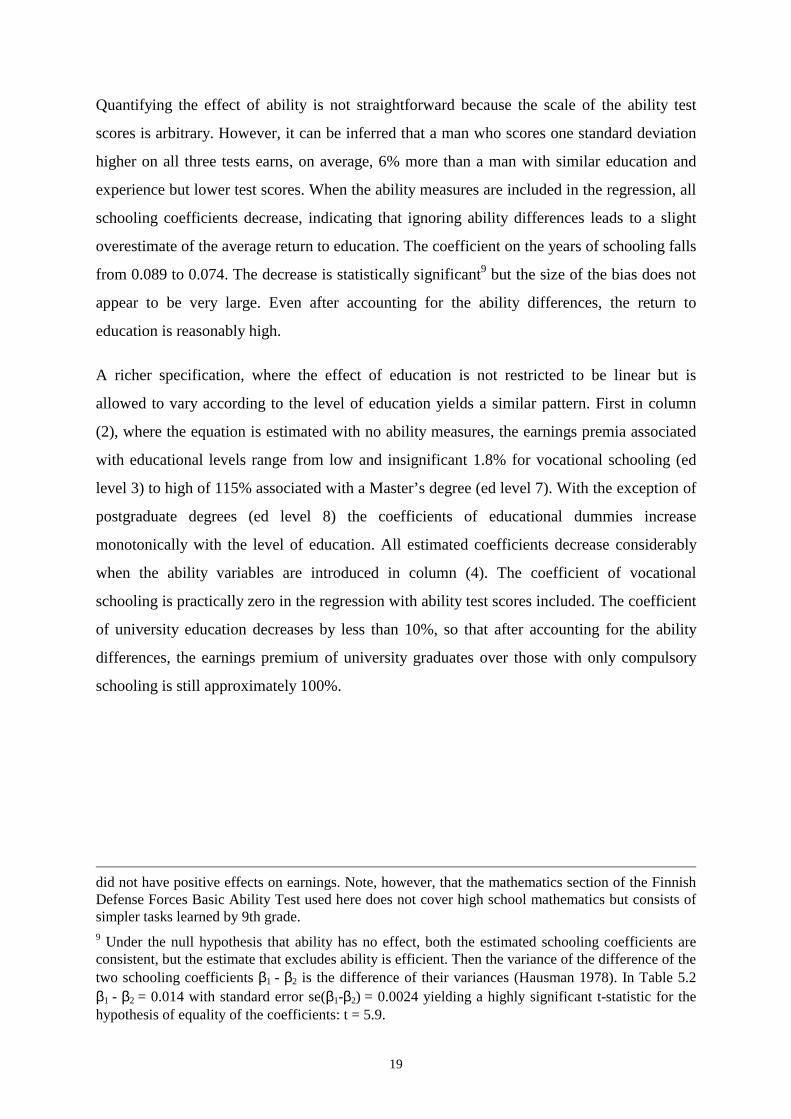
Quantifying the effect of ability is not straightforward because the scale of the ability test

scores is arbitrary. However, it can be inferred that a man who scores one standard deviation

higher on all three tests earns, on average, 6% more than a man with similar education and

experience but lower test scores. When the ability measures are included in the regression, all

schooling coefficients decrease, indicating that ignoring ability differences leads to a slight

overestimate of the average return to education. The coefficient on the years of schooling falls

from 0.089 to 0.074. The decrease is statistically significant9 but the size of the bias does not

appear to be very large. Even after accounting for the ability differences, the return to

education is reasonably high.

A richer specification, where the effect of education is not restricted to be linear but is

allowed to vary according to the level of education yields a similar pattern. First in column

(2), where the equation is estimated with no ability measures, the earnings premia associated

with educational levels range from low and insignificant 1.8% for vocational schooling (ed

level 3) to high of 115% associated with a Master’s degree (ed level 7). With the exception of

postgraduate degrees (ed level 8) the coefficients of educational dummies increase

monotonically with the level of education. All estimated coefficients decrease considerably

when the ability variables are introduced in column (4). The coefficient of vocational

schooling is practically zero in the regression with ability test scores included. The coefficient

of university education decreases by less than 10%, so that after accounting for the ability

differences, the earnings premium of university graduates over those with only compulsory

schooling is still approximately 100%.

did not have positive effects on earnings. Note, however, that the mathematics section of the FinnishDefense Forces Basic Ability Test used here does not cover high school mathematics but consists ofsimpler tasks learned by 9th grade.9 Under the null hypothesis that ability has no effect, both the estimated schooling coefficients areconsistent, but the estimate that excludes ability is efficient. Then the variance of the difference of thetwo schooling coefficients β1 - β2 is the difference of their variances (Hausman 1978). In Table 5.2β1 - β2 = 0.014 with standard error se(β1-β2) = 0.0024 yielding a highly significant t-statistic for thehypothesis of equality of the coefficients: t = 5.9.

20

It can be argued that the ability measured by the tests taken while in the army are affected by

the schooling completed before the test and, therefore, the effect of ability can not be

distinguished from the effect of schooling. After all, at least the tests for mathematical and

verbal ability measure skills that are taught in school. However, the inclusion of ability

measures in the regression has an effect also on the estimated return to university education

which occurs mainly after the test. In any case, the army ability test scores are less dependent

on prior schooling than other more school-related measures of ability such as school report

cards or final examination results, which are more or less measures of the quality of

schooling. Compared with the alternatives, the army tests are more independent and arguably

closer measures of the abilities rewarded in the labor market.10 In addition, only the results of

the matriculation examination would be comparable across schools. However, in late 1960’s,

when the men in this study finished their secondary schooling, only approximately 25% of the

age group stayed at school until the matriculation examination, i.e. finished twelve years of

general education (Kivinen and Rinne 1995). Thus, the examination results would only cover

the upper tail of the schooling distribution.

2.4 Effects of endogeneity of education

The schooling decision is at least in part a result of optimizing behavior of individuals or their

parents. This behavior is based on expected outcomes of different choices, i.e. some

anticipated earnings functions. To the extent that unobservable (to the econometrician)

‘errors’ of ex-post and ex-ante earnings functions are correlated, they will induce a correlation

between schooling and these unobservable disturbances (Griliches 1977). Controlling for

measured ability differences is not sufficient for unbiased estimation, because this correlation

may be caused by other unobserved variables.

In this section I present a set of estimation results of earnings equations, where schooling is

treated as an endogenous explanatory variable. Family background variables are used as

10 This argument is supported by Bishop (1994) who found that high-level academic competencies inscience and mathematics had no positive effect on earnings of young men. Also Blackburn andNeumark (1995) found that “academic test scores” did not have a significant effect on earnings while“nonacademic tests”, particularly, “numerical operations” and “auto and shop information”components of the Armed Services Vocational Aptitude Battery had a significant positive effect onearnings.

21

instruments that can be excluded from the earnings equation. It is assumed that family

background has no direct effect on earnings, but only affects earnings through its effect on

schooling. If education is endogenous with respect to earnings, the instrumental variable

estimates are consistent, while the ordinary least squares estimates are not. Estimations are

performed using two-stage least squares, assuming that years of schooling is a continuous

variable. For comparison, a selectivity model with an ordered probit selection rule that

captures the discrete nature of the schooling choice is also estimated.

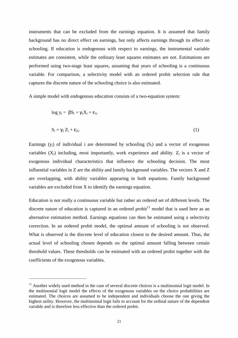
A simple model with endogenous education consists of a two-equation system:

log yi = βSi + γ1Xi + ε1i

Si = γ2 Zi + ε2i. (1)

Earnings (yi) of individual i are determined by schooling (Si) and a vector of exogenous

variables (Xi) including, most importantly, work experience and ability. Zi is a vector of

exogenous individual characteristics that influence the schooling decision. The most

influential variables in Z are the ability and family background variables. The vectors X and Z

are overlapping, with ability variables appearing in both equations. Family background

variables are excluded from X to identify the earnings equation.

Education is not really a continuous variable but rather an ordered set of different levels. The

discrete nature of education is captured in an ordered probit11 model that is used here as an

alternative estimation method. Earnings equations can then be estimated using a selectivity

correction. In an ordered probit model, the optimal amount of schooling is not observed.

What is observed is the discrete level of education closest to the desired amount. Thus, the

actual level of schooling chosen depends on the optimal amount falling between certain

threshold values. These thresholds can be estimated with an ordered probit together with the

coefficients of the exogenous variables.

11 Another widely used method in the case of several discrete choices is a multinomial logit model. Inthe multinomial logit model the effects of the exogenous variables on the choice probabilities areestimated. The choices are assumed to be independent and individuals choose the one giving thehighest utility. However, the multinomial logit fails to account for the ordinal nature of the dependentvariable and is therefore less effective than the ordered probit.

22

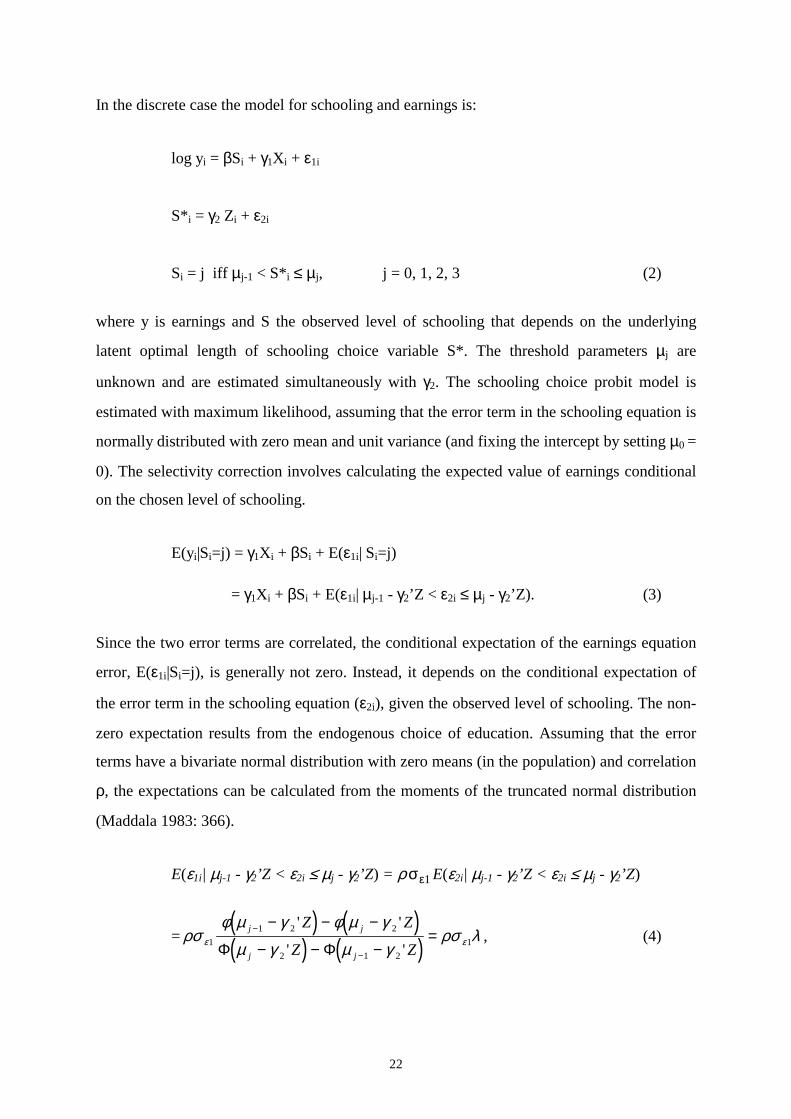
In the discrete case the model for schooling and earnings is:

log yi = βSi + γ1Xi + ε1i

S*i = γ2 Zi + ε2i

Si = j iff µj-1 < S*i ≤ µj, j = 0, 1, 2, 3 (2)

where y is earnings and S the observed level of schooling that depends on the underlying

latent optimal length of schooling choice variable S*. The threshold parameters µj are

unknown and are estimated simultaneously with γ2. The schooling choice probit model is

estimated with maximum likelihood, assuming that the error term in the schooling equation is

normally distributed with zero mean and unit variance (and fixing the intercept by setting µ0 =

0). The selectivity correction involves calculating the expected value of earnings conditional

on the chosen level of schooling.

E(yi|Si=j) = γ1Xi + βSi + E(ε1i| Si=j)

= γ1Xi + βSi + E(ε1i| µj-1 - γ2’Z < ε2i ≤ µj - γ2’Z). (3)

Since the two error terms are correlated, the conditional expectation of the earnings equation

error, E(ε1i|Si=j), is generally not zero. Instead, it depends on the conditional expectation of

the error term in the schooling equation (ε2i), given the observed level of schooling. The non-

zero expectation results from the endogenous choice of education. Assuming that the error

terms have a bivariate normal distribution with zero means (in the population) and correlation

ρ, the expectations can be calculated from the moments of the truncated normal distribution

(Maddala 1983: 366).

E(ε1i| µj-1 - γ2’Z < ε2i ≤ µj - γ2’Z) = ρσε1 E(ε2i| µj-1 - γ2’Z < ε2i ≤ µj - γ2’Z)

=( ) ( )( ) ( )ρσ

φ µ γ φ µ γ

µ γ µ γρσ λε ε1

1 2 2

2 1 21

j j

j j

Z Z

Z Z−

−

− − −

− − −=

' '

' 'Φ Φ, (4)

23

where σ ε1 is the standard error of the disturbance term in the earnings equation and φ(.) and

Φ(.) are, respectively, the density function and the distribution function of the standard

normal distribution.

Estimation resultsThe results of the first stage regression of schooling on ability and family background

variables are presented in Table 4. The reduced form least squares and ordered probit

coefficients are not directly comparable, since in the least squares equation, the dependent

variable is years of schooling, while in the ordered probit it is a discrete level of schooling.

However, the results are qualitatively similar with the father’s education and ability variables

having a highly significant impact on the length of schooling. The family background

variables that are to be excluded from the earnings equation are jointly significant in the

schooling equation and can, therefore, be used as instruments for schooling.12 The effect of

ability on schooling choice can be calculated from the parameter estimates of the reduced-

form OLS equation in the same way as the effect of ability on earnings in section 2.3. One

standard deviation increase in all the test scores increases schooling by 0.6 years. The impact

calculated using coefficients from a regression of schooling on family background and ability

variables only, without controlling for the other covariates of the earnings equation, is 1.2

years. The high predictive power of reduced form least squares is caused partly by inclusion

of earnings equation covariates, especially work experience.

12 Father’s income was originally also used as an instrument but since it was insignificant in theschooling equation and caused problems with the specification tests in the earnings equation, it wasswitched to the set of explanatory variables in the earnings equation. Father’s income apparently hasalso a direct effect on earnings.

24

Table 4 First stage regressions for schoolingReduced form OLSa Ordered probit

coefficient standard error coefficient standarderror

Intercept 17.612 0.780 -1.721 0.130Math test 0.019 0.005 0.039 0.006Verbal test 0.038 0.007 0.036 0.006Analytical test 0.013 0.009 0.021 0.009Father upper white-collar 0.323 0.231 0.395 0.177Father lower white-collar 0.133 0.130 0.234 0.127Father university educ. 0.991 0.259 0.971 0.231Father upper voc. educ. 0.507 0.161 0.415 0.156Father vocational educ. 0.078 0.143 0.217 0.129µ1 1.255 0.060µ2 2.098 0.077µ3 2.522 0.086µ4 2.749 0.092N 1016 1016F-test for excluded instrumentsb F(5,997)=9.53

p=0.00R squared 0.73Log likelihood -1237a All the equations include a set of dummy varaibles indicating if an individual was missing from anyof the census years. Reduced form OLS equation also includes all the covariates of the earningsequation.b The instruments that are to be excluded from the earnings equation are: indicator variables offather’s socio-economic status (upper white-collar, lower white-collar) and father’s education(university, upper vocational, vocational).

The estimation results from the different earnings equation specifications are reported in

Table 5. In the first column, the equation of Table 3, column (3) is re-estimated with ordinary

least squares using only the observations with nonmissing family background variables to

ensure that the difference between the OLS and IV estimates is not caused by sample

selection. The results in this subsample are not very different from the full sample estimates.

25

Table 5 Wage equations with endogenous education. Dependent variable is log annualearnings.

OLS IV (2SLS)a IV (2SLS)a selectivitycorrectedb

(1) (2) (3) (4)Intercept 10.08 8.69 9.10 9.47Years of education 0.081

(0.007)0.157

(0.017)0.129

(0.018)0.124

(0.013)Math test 0.003

(0.001)0.001

(0.001)0.002

(0.001)0.000

(0.001)Verbal test 0.001

(0.001)-0.003(0.002)

-0.001(0.002)

-0.002(0.002)

Analytical test 0.002(0.002)

0.001(0.002)

0.001(0.002)

0.001(0.002)

Experience 0.057(0.025)

0.109(0.034)

0.089(0.034)

0.081(0.028)

Experience squared -0.001(0.001)

-0.002(0.001)

-0.002(0.001)

-0.002(0.001

Log father’s income 0.014(0.005)

0.014(0.005)

λc -0.097(0.024)

N 1016 1016 1016 1016R squared 0.40 0.33 0.38 0.42Hausman testd t=2.50

p=0.01t=1.53p=0.12

Overidentification test χ2(5)=13.05p=0.02

χ2(4)=5.60p=0.23

The estimated equations also include same additional dummy variables for region and sector as table3 as well as indicators for missing data on any census. Standard errors are in parentheses.a The set of instruments that are excluded from the earnings equation includes dummy variables forfather’s education, father’s socioeconomic status and the place of residence in 1970 (See table 4). Incolumn (2) the set of instruments also includes father’s income while in column (3) father’s income isamong the regressors.b Calculating standard errors in the ordered probit is rather complicated. The residuals of the orderedprobit equation come from several truncated distributions. The correction used here is programmed inthe LIMDEP manual, p. 628 (Greene 1991).c Inverse Mills’ ratio, E(ε2 |S=j).d Test for the hypothesis that the OLS and IV coefficients are equal, performed by testing with the t-test the significance of the coefficients of the fitted values from the first-stage instrumental variablesregression in the log wage equation estimated with ordinary least squares. (Davidson and MacKinnon1993: 239)

26

The results from the instrumental variable estimation are presented in columns (2) and (3). In

column (2), the set of excluded instruments contains all the family background variables. The

schooling coefficient rises to almost 0.16 and schooling appears to be endogenous according

to the Hausman test. However, overidentification restrictions requiring that all instruments

are orthogonal to the earnings equation error are rejected.13 A prime candidate for a nonvalid

instrument is the father’s income which appears to have a direct effect on the son’s earnings.

When the father’s income is included in the earnings equation in column (3), the

overidentification restrictions are not rejected. The return to schooling estimate is now 0.129,

which is still clearly higher than the OLS-estimate of 0.081 but the Hausman test no longer

rejects the null hypothesis of equality of OLS and IV coefficients. The difference between IV

and OLS estimates is similar in magnitude to the estimates of Card (1993) but somewhat

smaller than in Harmon and Walker (1995). It is also interesting to note that the coefficients

of the ability variables decrease and lose their significance in the IV estimation.

Estimation of the selectivity-corrected earnings equation with the ordered probit selection

function in column (4) produces an estimate for the return to education that is also higher than

the OLS estimate. Endogeneity is supported by the significance of the selectivity correction

term λ. The estimate for λ is negative, which implies that the least squares estimates are

biased downwards.

13 The essential idea of the test is that, after controlling for the other covariates, the excludedinstruments should have no explanatory power in the earnings equation. The easiest way to performthis overidentification test is to regress the residuals from the two-stage least squares estimation onall the included explanatory variables and the excluded instruments. It can be shown that under thenull hypothesis of no correlation between the instruments and the error term of the earnings equation,nR2 from this regression is asymptotically χ2(l-k)-distributed, where l-k is the number ofoveridentification restrictions (Davidson and MacKinnon 1993).

27

So far the topic of this section has been the endogeneity of education. However, if the number

of years spent in school is endogenous, work experience, defined as the number of years at

work after school, must also be endogenous.14 Table 6 presents estimation results that are

consistent when experience is endogenous. In the first two columns, work experience is

replaced with age which can safely be treated as an exogenous variable. The interpretation of

the coefficient on education is now the net effect of spending an additional year in school

rather than gaining work experience. Here the schooling coefficient from the instrumental

variable regression exceeds the OLS estimate by almost 60%. In column (3) the equation is

estimated with two-stage least squares treating experience as endogenous and using age and

age squared as additional instruments. The resulting schooling coefficient is 0.11, only

slightly lower than in Table 5 where experience was treated as exogenous. Interestingly, the

coefficient of experience also decreases and is no longer significant at conventional levels.

14 A more convincing test for the endogeneity of experience would require information on actualyears of work experience. Since labor supply is expected to depend on wages, accumulated laborsupply will depend on an individual’s history of wages. Fixed components in the wage equation errorcould lead to current experience being correlated with the current error. As schooling and experienceare correlated, inconsistency in the experience coefficient estimate can carry over to the schoolingcoefficient estimate (Blackburn and Neumark 1995). However, treating work experience asendogenous may not be irrelevant even when information is available only on potential workexperience. The measure of work experience depends on the length of schooling. If the length ofschooling is endogenous, the work experience measure may also be correlated with the error term.

28

Table 6 Wage equations with endogenous education and experience.Dependent variable is log annual earnings.

OLSage proxyingexperience

IV (2SLS)age proxyingexperience

IV(2SLS)endogenousexperiencea

(1) (3) (3)Intercept 10.17 9.00 9.95Years of education 0.066

(0.005)0.104

(0.022)0.110

(0.021)Math test 0.003

(0.001)0.001

(0.002)0.001

(0.002)Verbal test 0.001

(0.002)-0.002(0.002)

-0.001(0.002)

Analytical test 0.002(0.002)

0.001(0.002)

0.001(0.002)

Log father’s income 0.016(0.004)

0.014(0.005)

0.014(0.005)

Age 0.013(0.083)

0.072(0.092)

Age squared -0.000(0.001)

-0.001(0.001)

Experience 0.033(0.073)

Experience squared -0.001(0.002)

N 1016 1016 1016R squared 0.41 0.37 0.38Hausman test t=1.79

p=0.07F(3,998)=1.42

p=0.23b

Overidentification test χ2(4)=3.91p=0.42

χ2(4)=4.33p=0.36

The estimated equations also include same additional dummy variables for region and sector as table3, as well as indicators for missing data on any census. Standard errors are in parentheses.The set of instruments (for both schooling and experience) includes dummy variables for father’seducation and father’s socioeconomic status.a In column 3 age and age squared are used as additional instruments.b Joint test of significance for the fitted values of schooling and experience from the first-stageregression in the log earnings equation.

While the returns to years of education give an impression of the average effects of education,

it may be more meaningful to study the returns to educational credentials. The return to a year

in school may vary according to the level of schooling. A year at a university is not equivalent

to a year in a vocational school. And, since the highest level of completed education is the

information that is actually recorded in the data, it is probably more reliable than an

artificially constructed measure of years of education.

29

Table 7 shows the results obtained when schooling is measured by the highest degree

completed. In the first column are the OLS estimates for the subsample with non-missing

family background information. In column (2) selectivity correction is applied using an

ordered probit selection function. Columns (3) and (4) repeat the analysis using wider

educational categories classifying levels 4 and 5 as upper vocational education and levels 6, 7

and 8 as university education. This grouping is used in estimating both selection and earnings

functions.

The reference category in the equations of Table 7 is individuals with only a compulsory

education. According to the OLS estimation, there are significant returns to all levels of

education except vocational schooling the effect of which is practically zero. These results are

similar to the full sample estimates.

The selectivity-corrected estimation results in column (2) again indicate an increase in the

estimated effect of education when the endogeneity of education is taken into account.

According to these estimates, a man with vocational schooling earns about 7 % more and a

man with a university degree about 140% more than he would have earned had he started

working directly after compulsory school.

The same pattern is visible also in columns (3) and (4) where education levels are not as

narrowly defined. Selectivity correction leads to a systematic although not significant increase

in estimated returns to educational credentials. The selectivity correction term is negative but

insignificant in both columns (2) and (4).

30

Table 7 Returns to qualifications. Dependent variable is log annual earningsOLS Selectivity

correctedOLS Selectivity

corrected(1) (2) (3) (4)

Intercept 10.64 10.67 10.82 10.85Ed level 3a 0.013

(0.022)0.067

(0.050)-0.005(0.022)

0.047(0.051)

Ed level 4 a 0.176(0.030)

0.265(0.079)

0.174 0.265

Ed level 5 a 0.281(0.043)

0.392(0.101)

(0.030) (0.084)

Ed level 6 a 0.425(0.061)

0.543(0.115)

0.569 0.702

Ed level 7-8 a 0.727(0.059)

0.873(0.135)

(0.052) (0.127)

Math test 0.003(0.001)

0.002(0.002)

0.003(0.001)

0.002(0.002)

Verbal test -0.001(0.001)

-0.002(0.002)

-0.000(0.001)

-0.002(0.002)

Analytical test 0.003(0.002)

0.002(0.002)

0.003(0.002)

0.003(0.001)

Experience 0.078(0.025)

0.080(0.025)

0.062(0.025)

0.063(0.025)

Experience squared -0.002(0.001)

-0.002(0.001)

-0.002(0.001)

-0.002(0.001)

λb -0.042(0.035)

-0.041(0.035)

N 1016 1016 1016 1016R squared 0.45 0.46 0.44 0.44Equations also include dummy variables for region and sector as well as a set of dummy varaiblesindicating if an individual was missing from any of the census years. Standard errors are inparentheses.a Comparison to the reference group “only compulsory education”.b Inverse Mills’ ratio, E(ε2 |S=j).

According to all the estimation results reported above, two-stage methods that take into

account the endogeneity of education produce systematically higher estimates for the effect of

education on earnings. This result implies that there is a negative correlation between

schooling and the earnings equation residual. This is a rather nonintuitive result; common

sense would suggest that unobserved ‘good’ characteristics should have a positive effect on

both earnings and schooling. Hence, the correlation between the residuals in the earnings

equation and the schooling equation should be positive. However, the estimation results

reported above as well as in previous studies based on the IV approach (Card 1993, Harmon

and Walker 1995) suggest the opposite.

31

2.5 Conclusion

Since individuals with different amounts of schooling generally differ also by other observed

and unobserved characteristics, ordinary least squares estimates based on comparison across

individuals may not reflect the true returns to schooling. In this paper I estimate returns to

education controlling for individual abilities by including ability test scores in the earnings

equations. I also treat education as endogenously determined or erroneously measured and use

family background variables as instruments for education.

The first question addressed in this paper concerns the effect of cognitive abilities, as

measured by the army test scores in 1970. These abilities are found to have a significant and

fairly large effect both on the choice of the length of schooling and on subsequent earnings.

Also, ignoring individual ability differences apparently overstates the profitability of

education, although the bias in the estimated return to years of schooling is not very large.

Introducing ability measures in the earnings equation decreases the estimated effect of years

of schooling on earnings from 9.3% to 7.7%

Taking into account the endogeneity of schooling suggests, however, that ordinary least

squares estimates are subject to a downward bias. Even after controlling for ability

differences, estimates using instrumental variables or selectivity correction techniques

produce estimates of the return to education in the range of 11-13%, significantly higher than

ordinary least squares estimates. These estimates are similar to those obtained by Card (1993)

and Ashenfelter and Krueger (1994) with U.S. data and Harmon and Walker (1995) with

U.K. data. The results suggest that the unobservable disturbances in the equations that

determine schooling and earnings are negatively correlated. Those who have completed

unexpectedly high amounts of schooling, given their family background and ability test

scores, are those who, for whatever reason, have lower than average initial earnings capacity.

There are at least three distinct explanations for the difference between ordinary least squares

and instrumental variables estimates. First, the least squares estimates may be downward

biased because of measurement error in schooling. Instrumental variable estimates are

consistent also in the presence of measurement errors. Second, the excluded instruments may

also have a direct effect on earnings. While overidentification tests generally did not reject the

hypothesis that family background can legitimately be excluded from the earnings equation,

the possibility of misspecification, that would bias the instrumental variable estimates

32

upwards, remains. Third, optimizing behavior by individuals may result in a correlation

between optimal schooling and the earnings equation error which leads to a bias in the OLS

estimates.

There is no clear-cut test to discriminate between these explanations. However, it appears

unlikely that measurement error could fully explain the difference between OLS and IV

estimates. In survey data, the reliability of schooling measures is typically estimated to be

around 90% (Ashenfelter and Krueger, 1994), which would attenuate the schooling

coefficient by 10% in a bivariate regression with schooling as the only explanatory variable.

In the administrative data used here, measurement error is likely to be smaller. When the

estimated equation includes several correlated variables that may all be erroneously

measured, the effect of measurement errors on estimates is much more complicated, but the

measurement error in schooling would have to be very large to induce a bias of the magnitude

found here.

However, it is tempting to note that the difference between IV and OLS estimates is in

accordance with models of the optimal choice of schooling. Schooling is cheaper for

individuals who have less income to forego while in school and, therefore, the optimal

amount of schooling is larger. In terms of Griliches (1977), optimized schooling and the

unobserved disturbance in the earnings equation may be negatively correlated if there is also

“another unmeasured individual income generating factor unrelated to ability (for example,

motivation or energy)” which only increases potential earnings and therefore marginal costs

of schooling with no effect on the marginal return to schooling. A negative correlation

between schooling and the error term is likely to bias OLS estimates downward.

33

References

Angrist, J. and A. Krueger, 1991, Does compulsory school attendance affect schooling and earnings?

The Quarterly Journal of Economics 106(4).

Angrist, J. and A. Krueger, 1992, Estimating the payoff to schooling using the Vietnam era draft

lottery, NBER Working Papers, no. 4067.

Ashenfelter, O. and A. Krueger, 1994, Estimates of the economic return to schooling from a new

sample of twins, American Economic Review 84(5).

Asplund, R., 1993, Essays on human capital and earnings in Finland, The Research Institute of the

Finnish Economy, Series A18.

Bishop, J., 1994, Schooling, learning and worker productivity, in: R. Asplund, ed., Human capital

creation in an economic perspective (Physica-Verlag, Helsinki).

Blackburn, M. and D. Neumark, 1993, Omitted-ability bias and the increase in the return to

schooling, Journal of Labor Economics 11(3).

Blackburn, M. and D. Neumark, 1995, Are OLS estimates of the return to schooling biased

downward? Another look, The Review of Economics and Statistics 77(2).

Butcher, K. and A. Case, 1994, The effect of sibling sex composition on women’s education and

earnings, The Quarterly Journal of Economics 109(3).

Card, D., 1993, Using geographic variation in college proximity to estimate the return to schooling,

NBER Working Papers, no. 4483.

Card, D., 1994, Earnings, schooling and ability revisited, NBER Working Papers, no. 4832.

CSO, 1991, Väestölaskentojen pitkittäistiedosto 1970 - 1985, Käsikirja (Handbook of longitudinal

census file 1970 - 1985) (Central Statistical Office of Finland, Helsinki).

Davidson, R. and J. MacKinnon, 1993, Estimation and inference in econometrics (Oxford University

Press, Oxford).

Greene, W., 1991, LIMDEP. User’s manual and reference guide (Econometric Software Inc.).

Greene, W., 1993, Econometric analysis, 2 ed. (Macmillan, New York).

Griliches, Z. and W. Mason, 1972, Education income and ability, Journal of Political Economy, 80(2).

Griliches, Z., 1977, Estimating the returns to schooling: Some econometric problems, Econometrica,

45(1).

34

Harmon, C. and I. Walker, 1995, Estimates of the economic return to schooling for the UK, American

Economic Review, 85(5).

Hausman, J., 1978, Specification tests in econometrics, Econometrica, 46.

Heckman, J., 1979, Sample selection bias as a specification error, Econometrica, 47(1).

Kivinen, O. and R. Rinne, 1995, Koulutuksen periytyvyys. Nuorten koulutus ja tasa-arvo Suomessa

(The inheritance of schooling. Schooling and equality in Finland), Statistics Finland, Education

1995:4.

Maddala, G., 1983, Limited-dependent and qualitative variables in econometrics (Cambridge

University Press).

Miller, P., C. Mulvey and N. Martin, 1995, What do twin studies reveal about the economic returns to

education? A comparison of Australian and U.S. findings, American Economic Review, 85(3).

Scheinin, M., 1987, Constitution, conscription and conscientious objection in Finland, in: J.

Väänänen, K. Kinnunen, eds., Youth and conscription (Suomen Rauhanliitto - YK-yhdistys,

Helsinki).

Taubman, P. and T. Wales, 1973, Higher education, mental ability and screening, Journal of Political

Economy, 81(1).

White, H., 1980, A heteroskedasticity-consistent covariance matrix estimator and a direct test for

heteroskedasticity, Econometrica, 48.

Willis, R., 1986, Wage determinants: A survey and reinterpretation of human capital earnings

functions, in: O. Ashenfelter and R. Layard, eds., Handbook of Labor Economics, Vol. 1 (Elsevier).

35

Chapter 3

Estimating heterogeneous treatment effects

in the Becker schooling model1

Abstract

In this paper, we provide evidence that the rate of return to schooling varies acrossindividuals and this variation is responsible for much of the variation in the length ofschooling. The varying returns imply a random coefficient model of earningsdetermination. We show that instrumental variable estimators still consistentlyestimate the average return to schooling under reasonable assumptions and that theIV-estimates are almost identical to more general control function estimates. Ourmaximum likelihood estimates imply that variation in the returns to schooling isrelated to ability differences while family background only affects the discount rates.

Keywords: Returns to schooling, random coefficient models, IV-estimators

3.1 Introduction

The empirical literature on program evaluation, including the impressive body of literature on

returns to schooling, typically frames selection bias as an omitted variable problem. If

treatment, the degree of participation in a social program, is positively or negatively

correlated with unobservables that affect the outcome of interest, then ordinary least squares

estimates of the average effect of treatment will absorb the effects of these unobservables, and

will be biased accordingly. This selection problem will occur when program participation is

endogenously determined by the same unobservable factors which influence the outcome.

Given this omitted variable problem, instrumental variable estimators or appropriate two-step

selection correction methods consistently estimate treatment effects.

1 Joint work with Karen Conneely.

36

However, the traditional concept of selection bias as a problem of omitted variables is overly

narrow. According to economic theory, individual participation decisions should weight

equally the costs and benefits of participation. The simple selection problem described above

reflects only cost-based selection. As we discuss below, the endogeneity problem due to

selection based on variable benefits is different and more severe.

Variation in benefits implies positive selection, since individuals with higher benefits to

participation in a program are more likely to participate, ceteris paribus. In this case, the

endogenous treatment variable is influenced by its own coefficient, yielding an endogeneity

problem that is not accounted for in most selection-correction models. This problem will exist

unless the benefits of the program are truly constant across individuals. However, the

assumption of constant benefits is probably unrealistic. It seems likely that individuals who

are heterogeneous in all other dimensions, including the observed regressors, unobserved

earnings potential, and costs of participation, will also vary in their potential to benefit from a

social program.

In the empirical literature, the benefits to a program are commonly treated as a single

population parameter to be estimated, even when it is accepted that benefits vary. Often it is

more feasible to estimate a single parameter of interest, such as the average benefit to a year

of education, than an entire distribution of benefits. However, estimates of the average benefit

of the treatment may be biased upward if actual benefits vary.

Still, much of the theoretical literature acknowledges the presence of heterogeneity in returns

without addressing the selection bias implied by this heterogeneity. Angrist and Imbens

(1995) show that the IV-method can be used to calculate average causal responses to

treatment even in the case when the responses vary between individuals. Implicit in their

analysis, however, is the assumption that the expected responses do not affect the choice of

the level of treatment. In a related paper, Imbens and Angrist (1994) show that the IV-

estimates identify local average treatment effects, that is, the average effect of treatment on

the people who were induced to change their participation status by a change in the

instrument. Again, individual variation in treatment effects is acknowledged but the

possibility that this variation may influence participation is not.

37

Heckman (1995,1997) shows that instrumental variables estimates of treatment effects are

consistent only if (a) the effect of treatment is the same for everyone (conditional on

observables) or (b) treatment effects are variable across people but do not affect the decision

to participate in the program. While condition (a) is typically assumed in the empirical

literature and condition (b) is implicitly assumed in the work by Angrist and Imbens (1995),

Heckman argues that neither of these assumptions is realistic. Condition (b), the less

restrictive of the two conditions, requires that the persons being studied do not have better

information than the econometrician on the likely effects of the program. Since this

assumption requires extremely rich data available to the econometrician, Heckman concludes

that the method of instrumental variables is likely to fail in estimating the effects of treatment

on the treated.

Heckman and Robb (1985) and Garen (1984) discuss the use of control function estimators,

which include terms that proxy the variable component of the coefficient. These estimators

generally require assumptions that are somewhat stronger than those conventionally used to

guarantee consistency of the IV-estimators, but are weaker than the more general IV-

assumptions discussed above. In the case of dichotomous treatment these estimators are

usually dependent on distributional assumptions and hence very different from their IV

counterparts. In the case of continuous treatment with linearity assumptions (as in Garen

1984), the appropriate control function estimator is simply a more general IV-estimator

requiring only slightly weaker assumptions.

Under this framework, we consider the consistency of instrumental variables estimation of

average treatment effects when the effects may vary across individuals, and analyze the

resulting estimation problems in the familiar context of estimating the returns to schooling. In

section 3.2 we present the continuous-treatment evaluation problem in terms of the Becker

schooling model, yielding a variant of the random coefficients model. Section 3.3 descibes

the data. The IV and control function estimates are presented in section 3.4. Finally, in

Section 3.5 we use maximum likelihood to estimate a joint model of wage determination and

schooling. Section 3.6 wraps up with a brief conclusion.

38

3.2 Variable returns to schooling and related estimation problems

A common example of an estimation problem of the effects of continuous treatment is the

classic case of the returns to schooling. While most of the empirical literature on this topic

has not dealt with the possibility of individual variation in returns to schooling, the idea has

received attention in several more theoretical treatments of the topic. Variation in returns is

implicit in the dichotomous schooling choice model of Willis and Rosen (1977), who analyze

the decision to attend college. Card (1994), in a re-interpretation of Becker (1967), presents a

model of endogenous schooling determination where schooling choice is continuous and is

influenced by varying returns. This model is consistent with the stylized facts about the

determinants of schooling and the relation between schooling and earnings, predicting that

variation in family background and ability will have a strong effect on schooling choice and

that the relationship between schooling and log earnings is approximately linear.

We adopt Card’s version of the Becker model and assume that individuals choose schooling

to maximize a utility function (U) defined over average earnings (y) and years of schooling (S):1

U(y,S) = ln y - f(S) (1)

where f(S) is an increasing convex function representing the disutility of attaining schooling

level S. Individual opportunities can be summarized by a log-concave function y = g(S),

which represents the level of earnings available at each level of education. This yields the first

order condition for optimal schooling:

gg

f' (S)(S)

' (S)= . (2)

In the standard case ln y=a+bS and f(S)=rS, where b is the marginal return and r the marginal

cost. Now, the optimization problem is equivalent to maximizing discounted lifetime

earnings for infinitely lived individuals: g S e dt g S er

rt

S

rS

( ) ( )−∞ −

∫ = . The first-order condition

(2) above reduces to b=r, so optimal schooling equates the marginal rate of return to

schooling with the marginal cost of schooling or marginal rate of substitution between current

1 For a similar derivation see Ashenfelter and Rouse (1996).

39

and future earnings.2 If b and r are constant in schooling, the solution to the optimization

problem will be a corner solution: S*=0 if b<r; S*→∞ if b>r. An interior solution can only be

guaranteed with the assumption that either marginal returns or marginal costs vary with the

level of schooling.

As in Card (1994), we operationalize the model by assuming that marginal costs are

increasing linear functions of schooling. To keep our analysis simple, we diverge from Card’s

model with our assumption that marginal returns do not vary with schooling, although we will

relax and test this restriction when we estimate the model with maximum likelihood. To

allow for individual heterogeneity in marginal returns and marginal costs, we assume person-

specific intercepts but assume a homogenous slope for marginal costs:

gg

bi' (S)(S)

= (3)

f r kSi' (S) = + (4)

Equalizing marginal costs and benefits yields an optimal level of schooling for individual i:

Sb r

kii i* =−

(5)

In this model, schooling choices vary across individuals for two reasons: because individuals

have different rates of return to schooling (variation in bi), and because individuals have

different rates of substitution between schooling and future earnings (variation in ri). Card

(1994) speculates that variation in bi corresponds to variation in ability while variation in ri

corresponds to variation in access to funds or tastes for schooling. Denoting the population

means of bi and ri as b and r we can rewrite returns and costs as :

bi = b + νbi, (6)

2 We use the terms marginal costs and (marginal) discount rates interchangeably. Both refer to thederivative of function f (S) with respect to schooling. In our model, the discount rates and themarginal costs of schooling are not separately identified.

40

ri = r + νri. (7)

Integrating the marginal returns equation yields our implicit assumption of the standard log-

linear earnings equation for individual i:

ln yi = a + bi Si + ε. (8)

If marginal returns to schooling vary between individuals then the above equation can be

treated as a random coefficients model:

ln yi = a + ( b + νbi)Si + ε. (9)

Note that because schooling depends on the return, bi, there is positive correlation between Si

and its random coefficient. This variant of the random coefficients model is not commonly

dealt with in the literature. The textbook random coefficients model3 treats random

coefficients as white noise, assuming that there is no correlation between the random

individual component of the slope coefficient and any of the other regressors. In the textbook

case, the standard OLS or IV methods yield consistent, but inefficient estimates. However,

such a model is not a realistic descriptor of schooling choice if individuals have private

information about their ability to benefit from additional schooling.

The above random coefficient model can be rewritten as

Y = a + b S + (ε + νbS) = a + b S + U. (10)

The interesting parameter here is the average return to a year of schooling, b ,4 but the OLS

estimates of b will be inconsistent if S is correlated with the error term. In this case, the OLS

estimates will suffer from two separate types of bias since S may be correlated with both ε

and νbS.

3 See, for example, Greene (1993)4 Note that contrary to a discrete choice case, the average population return to education is theinteresting parameter when treatment is continuous. In a discrete choice case it might be moreinteresting to estimate the effect of treatment to some subpopulation actually receiving treatment. Inthe continuous case everyone receives treatment, but in varying intensities.

41

S and ε will be positively correlated if individuals with higher potential earnings tend to attain

more schooling, perhaps because of lower costs or disutilities of schooling (E(ενr) < 0). In

this case, the OLS estimates will overstate the return to schooling. If this were the only source

of bias (i.e. if νb=0) then consistent estimates of b could be obtained with instrumental

variables estimators or simple selection correction. For the IV estimates to be consistent, the

instrument Z must be correlated with the endogenous variable (S) but uncorrelated with the

error (U):

A1) E(S|Z) ≠ E(S);

A2) E(U|Z) = 0.

If benefits of the program are constant across individuals (νb=0), then U is simply ε, so these

conditions are met by variables which affect the costs of schooling but not earnings. Potential

instruments could include measures of family background, as well as variables which mimic

random assignment.

When benefits or the program vary, these conditions cannot be satisfied. In a population of

rational, well-informed individuals, those with a higher return to a year of schooling, should

attain more schooling than those with lower returns. Hence, S will be positively correlated

with νb, violating the condition E(U|Z) = E(ε + νbS |Z) =0. Also, A1 explicitly states that S

must be correlated with Z in some way, so ε + νbS is likely to depend on the instrument Z.

Using this argument, Heckman and Robb (1985) demonstrate the general inconsistency of

instrumental variables estimators in random coefficients models. Their proposed solution to

the random coefficient estimation problem is control function approach, similar to the two-

step procedure commonly used to correct for traditional selectivity bias. In this approach, the

participation decision is modeled to obtain consistent estimates of E[ε + νbS |S, Z], which are

then plugged into an OLS regression of earnings on schooling:

E[Y|S,Z] = a + b S + E[ε |S,Z] + S ⋅ E[νb |S,Z]. (11)

This approach requires that the conditional expectation of the unobservables, νb and ε, can be

specified up to unknown parameters in terms of the observables S and Z. This is usually done

42

by specifying the functional form of the participation decision and the relationships between

the unobservable terms. Since schooling is a roughly continuous variable, it seems natural to

specify a linear relationship between S and Z:

S = γ Z + η (12)

where γ ≠0 and η is uncorrelated with Z:

CF1) E(η|Z) =0 .

Depending on the assumptions one is willing to make about the conditional expectations in

(11) several estimation strategies are available. In a linear case the most common assumption

is that conditional expectations of the outcome equation are linear in η = S - γ Z.

CF2) E[ε |S, Z] = E[ε |η] = c η

E[νb |S, Z] = E[νb |η] = d η.

Given the relationship specified in CF2, the appropriate control function estimate of b would

be obtained by obtaining the OLS residuals �η from the reduced form schooling equation (12)

and estimating the following OLS regression:

Y = a + b S + λ1 �η + λ2 �η S5. (13)

Garen (1984) uses this control function approach to estimate the return to schooling in a

random coefficients framework, asserting that the IV estimates are inconsistent in this type of

model due to violation of the condition E[U|Z]=0. He specifies a model similar to the one

discussed here, except for the additional assumption of joint normality of the unobservables.

5 The standard errors from this regression will need to be corrected for the presence of estimatedregressors and heteroskedasticity of known form. Rewriting equation (13) as Y = X ’β + u, Var(β) =(X‘X)-1 (X‘VX + (X‘DZ) ση2(Z’Z)-1 (Z’DX)) (X‘X)-1, where D is a diagonal matrix containing thederivative of Y with respect to �η (in this model Di = λ1 + λ2 S). V is a diagonal matrix containing theestimated variance of the disturbance term u. In this model Vi = σε|η2 + 2Si σbε|η + Si

2σb|η2. Provided that

the disturbances are homoskedastic with respect to each other, Vi is a function of schooling only andcan be estimated using the predicted values from a regression of the squared residual from equation(13) on Si and Si

2.

43

This additional assumption is sufficient but overly strong for consistency of a control function

estimator. It not only generates conditions CF1 and CF2, but imposes homoskedasticity of all

unobservables. We will show below that this guarantees the consistency of the IV estimator

as well.

Note that if the final term were left out of the regression, that is, if λ2 were restricted to zero,

equation (13) would be equivalent to a simple two-step selection correction. When the

participation decision is linear, however, the two-step selection correction is numerically

equivalent to instrumental variables. Hence, the control function specified above is just a less

restrictive form of instrumental variables.

In addition to CF1 and CF2, the only extra condition required for consistency of the IV

estimator, using Z as the instrument, is the assumption that η is homoskedastic: E(η2|Z) = ση2.

This is obviously not satisfied in a discrete choice case with a linear probability model, but

may be quite reasonable in a continuous case. Given CF1, CF2, and homoskedasticity of η,

and using the law of iterated expectations

E(ε + νb S |Z) = E[E(ε + νb S |Z, η)|Z] = E[cη + dη(γZ+η)|Z]

= (c + dγZ) E[η|z] + dE[η2|Z] = dση2 = E(ε + νbS). (14)

As noted by Robinson (1989), E(U|Z) = E(U) is sufficient for consistent IV estimation of all

parameters in the earnings equation except the intercept term. The assumption deviates from

A2 only in that the error term is unconditionally biased; this bias is simply absorbed by the

intercept term and all other parameters can be estimated consistently with IV6.

So given the requirements for the control function estimator and the additional assumption of

homoskedasticity, IV estimator will consistently estimate all of the interesting parameters

even when schooling is correlated with its coefficient. If these assumptions can be reasonably

expected of a typical instrument, then this is good news for the multitude of instrumental

6 Wooldridge (1997) shows that the IV estimates are consistent in the random coefficient model using essentiallysimilar arguments. He also presents an alternative set of assumptions that could be applied to treatment if theparticipation choice follows a linear probability model.

44

variables estimates of the return to education. These assumptions are stronger than the usual

requirements for IV, and credible instruments are hard enough to find without the extra

restrictions. However, many of these assumptions are implied by other common (but stronger)

assumptions. For example, true independence of η and Z (as opposed to mean independence)

will guarantee homoskedasticity of η conditional on Z. Although stronger than necessary,

independence is often explicitly assumed in the theoretical literature since it yields

consistency results for a broader class of models. It is also implicit in most distributional

assumptions, including joint normality of unobservables, which also generates CF1 and CF2.

The control function estimator described above is slightly less restrictive in this case and will

be consistent under weaker conditions. However, as pointed out by Wooldridge (1997), the

gains to consistency from using a control function estimator may not be worth the extra

computation required, since the standard errors will need to be adjusted to reflect the two-

stage estimation process.

3.3 Data

3.3.1 BackgroundThis study utilizes a unique Finnish dataset of 37,000 young men who were performing their

military service in 1982. Since military service is compulsory in Finland, the sample contains

almost the entire 1962 birth cohort.7 This dataset includes scores from a battery of ability tests

performed during service. Statistics Finland has linked the army sample to a longitudinal file

of Finnish censuses which contains usual labor market information. The latest information

available on earnings and schooling is from 1994 administrative labor market records. Family

links are provided in the Finnish censuses, so the dataset also contains labor market

information on the parents of the men in the sample. Below several features of the dataset are

discussed in greater detail.

7 It is possible to postpone military service because of school enrollment and apply for service earlieras a volunteer. For this reason only about 70% of the sample were actually born exactly in 1962.

45

Test scores

The Finnish Defense Forces Basic Ability Test (Peruskoe 1) developed by the Finnish

Defense Forces Education Development Center has been administered since 1955 for all new

recruits at the beginning of their service. The ability test consists of three subtests measuring

verbal ability, analytical reasoning and mathematical reasoning.8 The raw scores of different

subtests are approximately normally distributed and range from 1 to 40. The army uses a

combined and scaled score in the selection of the rookies that are given officer training. In

this paper the scores are handled separately and are standardized to a mean of zero and unit

variance. Because the tests may partially reflect schooling attained, this analysis uses the

residual component of test scores that is not explained by education level at time of test. We

obtained these residuals by regressing the test scores on pre-test schooling, final schooling

level and family background variables. Then we subtracted from the test scores the

component that was explained by pre-test schooling. The component explained by post-test

schooling was left in, since it obviously could not influence the test scores.

Educational information

Schooling information in the Finnish data is based on the Register of Degrees and

Examinations compiled by Statistics Finland. The register is updated yearly with information

submitted directly by educational institutions. The data contains a five-digit code in which the

first digit indicates the level of education. For this analysis, degrees completed are converted

to years of schooling based on the Standard Classification of Education by Statistics Finland.9

Since the data is based on administrative reports it is free from the recall errors common in

survey data. The major problem with the data is that it has no record of schooling that did not

lead to a degree.

8 A more detailed description of the test items can be found in Uusitalo (1996).9 Statistics Finland classifies post-compulsory education into six levels according to the length ofeducation. Here individuals with no record on post-compulsory education are assigned to the lowestlevel (9 years) of schooling. For this analysis, an additional category was created splitting the highestlevel into licentiates and PhD’s. All other levels of education are coded according to the officialclassification, resulting in eight possible levels of education corresponding to 9, 11, 12, 14, 15, 17, 19and 21 years of schooling.

46

Earnings information

The earnings information in Finnish census data is based on income tax reports and is

collected directly from tax authorities. In this paper, annual pre-tax income from wages and

salaries are used as the earnings measure. As with education, this measure of earnings is

better than usual in that it is free from the usual reporting and recall errors. Unfortunately,

there is no reliable measure of hours worked so it is not possible to calculate an hourly wage.

Instead, log monthly earnings (calculated using annual income and available information on

months worked10) is used as the outcome variable.

Geographic information

To control for local labor market differences and other geographic factors that may influence

earnings and schooling, some specifications utilize information on place of residence in 1980,

when most of the men of the sample were 18 years old. We include indicators for geographic

region, residence in a city that has a university, and population of city of residence in 1980.

10 Months worked is calculated by subtracting months unemployed from months in the labor force.Unemployment data is based on unemployment records of Ministry of Labor and labor forceparticipation on pension registers. There is some measurement error in the months worked (averagemonthly wage decreases with months worked). To minimize the problem, observations reported ashaving worked less than six months are excluded from the analysis.

47

3.3.2 Descriptive statisticsThe analysis is restricted to men who are out of school and work full-time.11 Also excluded

are observations with reported monthly earnings below 2,000 marks and observations with

missing family background variables (father’s and mother’s education). As a result of these

restrictions, the effective sample is 22572 for most specifications. Table 1 presents some

descriptive statistics of this sample. Comparing the Finnish data to more commonly used

datasets with similar information content, such as the National Longitudinal Survey of Youth,

it can be concluded that these data have several advantages. The sample size is greater than in

comparable datasets. Reliance on administrative data ensures more accurate information on

schooling and earnings. The ability test score data is of comparable quality. The main

disadvantages of this dataset are its lack of information on hours and non-completed spells of

education.

Table 1. Descriptive statisticsVariable Mean Std Dev Minimum MaximumEarnings 1994 128742 57929 12000 1034721Calculated monthly wage (1994) 11229 4763 2000 86899

Years of schooling 1994 12.04 2.38 9 21Potential (Mincer ) experience (1994) 13.18 2.33 3 25

Calculated work experience (1994) 11.32 4.35 0.5 25.58

Age in 1994 32.22 1.52 29 41

Residual component of age 0.009 1.394 -5.407 9.075

Logic test score (normalized) 0.116 0.987 -2.186 2.641

Verbal test score (normalized) 0.114 0.980 -2.782 2.312

Math test score (normalized) 0.113 0.966 -3.807 2.783

Mother’s years of schooling (1980) 9.88 1.63 9 20

Father’s years of schooling (1980) 10.11 2.09 9 20

Mother’s earnings in 1980 27033 20032 0 283699

Father’s earnings in 1980 46380 39195 0 618291

Population of city of residence in 1980 73968 128972 <1000 483000

Living in a university city in 1980 0.255 0.436 0 1

N=22572

11 In 1994 Finland was going through the biggest recession of the century and the unemployment ratewas 18%. Excluding the unemployed from the sample is likely to reduce the estimates for the returnto schooling, since those with less schooling (and earnings) are more likely to be unemployed.

48

Table 2 presents results from several simple OLS regressions of log earnings on schooling.

The estimated return to schooling of 0.091 in Column (1), a conventional earnings function

using Mincer experience (age-schooling-7) as a proxy for true work experience, is consistent

with previous estimates using Finnish data (Asplund 1993). The model in Column (2) is the

same except a more accurate measure of potential experience is substituted for Mincer

experience. This measure is the amount of time lapsed since the last degree was received. In

Column (3) both measures are used, and they share the task of explaining wages pretty

equally.

Columns (5) - (8) include measures of family background and ability test scores in addition to

the simple Mincer specification. Including ability measures in the regression (Column (6))

reduces the return to schooling somewhat, from 0.085 in Column (4) to 0.079. All three

ability measures affect earnings positively, although the effect of the verbal test score is

insignificant. Of the three ability measures, the math test score has the largest direct impact

on earnings. The inclusion of parents’ education and earnings in the model (Columns (6) and

(7)) decreases the estimated return to schooling only slightly, even though parents’ earnings

and father’s schooling all have a clear positive effect on their sons’ earnings. In Column (6),

which includes parents’ schooling levels but not earnings, father’s schooling appears to have

a significant positive effect on earnings. However, with the addition of parents’ earnings and

ability (Column 8), the effect of father’s schooling is no longer significant and the effect of

mother’s schooling appears to be negative. Ability and parents’ earnings retain their positive

effect on wages in this specification.

49

Table 2. OLS estimates of the return to schooling(1) (2) (3) (4) (5) (6) (7) (8)

Schooling 0.091t=55.3

0.087t=61.9

0.096t=56.7

0.085t=60.9

0.079t=53.7

0.083t=57.7

0.083t=58.7

0.077t=51.7

Mincer experience 0.029t=17.4

0.018t=9.5

Calculated workexperience

0.014t=18.8

0.010t=11.9

0.014t=17.8

0.015t=19.2

0.014t=18.1

0.014t=18.6

0.015t=7.7

Math score 0.031t=7.8

0.030t=7.6

Verbal score 0.003t=0.9

0.003t=0.7

Logic score 0.013t=3.8

0.011t=3.3

Father’sschooling

0.008t=5.6

0.001t=0.8

Mother’sschooling

0.000t=0.04

-0.005t=-2.8

Father’s earnings(10 000 FIM)

0.006t=10.0

0.006t=7.7

Mother’s earnings(10 000 FIM)

0.007t=5.93

0.007t=5.3

Regional variables no no no yes yes yes yes yes

R squared 0.179 0.181 0.184 0.194 0.202 0.196 0.199 0.206

N=22572. T-statistics reported below coefficients.

50

3.4 Instrumental Variables and Control Function Estimation

3.4.1 Selection of InstrumentsThe OLS estimates in the previous section will be inconsistent as long as (a) earnings are

affected by other unobservable factors which are correlated with schooling or (b) the return to

schooling itself varies and individuals at least partially observe their own returns. Under

conventional assumptions, IV estimates will be consistent under (a) but not (b). In this case,

consistency of IV is dependent on stronger assumptions. A control function estimator that

explicitly accounts for the variation in return to schooling will be consistent under both (a)

and (b) under slightly weaker conditions. Both estimators require an instrument that exerts no

independent effect on earnings.

A good instrument must be highly correlated with the endogenous variable of interest

(condition IV1) and not be correlated with the error term in the outcome equation (condition

IV2). Two possible instruments available in the data are residence in a university city in 1980

and parents’ education. Residence in a university city is similar to other instruments that have

been used in the literature (see, for example, Card 1995b) and is generally considered to be a

credible instrument. Its appeal is that as long as other regional differences are controlled for,

it seems unlikely to affect earnings except through its effect on schooling. As for parents’

schooling, instruments based on family background are less credible in general because they

are likely to be correlated with unobservable determinants of earnings. Table 2 shows that

controlling for parents’ earnings, parents’ schooling has no direct effect on earnings, but this

does not prove that it meets condition IV2.

Both potential instruments for schooling satisfy condition IV1, and this can be verified easily.

Results from two sets of reduced form schooling regressions are presented in Table 3. Note

that since these regressions are the first stage of two stage least squares, all exogenous

variables from the earnings equation are included in the schooling equations and all

endogenous variables must be excluded. Naturally, any measure of experience which is based

on schooling will also be endogenous, so an instrument for experience is needed also. Age is

the usual candidate, but in this case age is slightly endogenous with respect to schooling, due

51

to selection into the sample.12 So in this analysis the instrument for experience is the residual

component of age with respect to schooling: the conditional means E(Age|Schooling) are

computed at each schooling level and are subtracted from actual age. Since the university city

instrument is only likely to be valid if other geographic characteristics are controlled for, a

full set of regional indicators is also included as well as the population of the city of residence

in 1980.

Looking at the first column of the first table, the family background and ability test scores are,

as expected, the most important determinants of schooling. Both mother’s and father’s

schooling have a highly significant positive effect on son’s schooling. An increase in either

mother’s or father’s schooling by one year is associated with approximately 0.1 year increase

in son’s schooling, even controlling for ability differences. Growing up in a city with a

university also increases the amount of education attained, although this effect is slight

compared to the others. The age residual also has only a slight effect, as it should. The next

two columns contain the first stage regressions for the two different kinds of experience. In

both cases, the age residual is a powerful determinant of experience, while all the predictors

of schooling have the expected negative effects on experience.

So, both parents’ schooling and university city have significant effects on schooling, meeting

condition IV1, but parents’ schooling has greater explanatory power. This leads to somewhat

of a tradeoff, since university city is probably more likely to meet condition IV2. In

identifying potential biases in IV estimates, condition IV2 is typically emphasized more than

condition IV1. Theoretically, the bias associated with a weak instrument that is just slightly

correlated with the error term (as it always will be in finite samples) could be greater than the

bias associated with a stronger instrument that is somewhat more correlated with the error

term (see Bound et al. 1995). On the other hand, Card (1998) shows that using family

background measures as instruments will lead to upward biased estimates.

A separate problem in instrument selection is that, if the returns are not constant, the

estimates do not necessarily reflect the average effects in the population. As shown in Angrist

12 The sample consists of men who served in the army 1982. About two thirds of the men were 20years of age at the beginning of their service. However, it is possible to postpone service or applyearlier as a volunteer. The most common reason for postponing service is continued schooling. Also,serving at 19 is very convenient for college-bound high school graduates. Therefore, both older andyounger cohorts had on average more schooling before entering the army than the 1962 birth cohort.

52

and Imbens (1995), the instrumental variables estimate is a weighted average of causal

responses to treatment (schooling) for those whose treatment status is affected by the

instrument. They point out that in the well-known study by Angrist and Krueger (1991), the

group with 8-12 years of schooling contributes the most to the estimates. In a related

argument, Card (1995) shows that college proximity has larger effects on those with low

predicted schooling. In this case IV estimates of the return to schooling based on college

proximity will be upward biased since they get disproportionately more weight from students

from poorer family backgrounds who face higher discount rates and, in optimum, higher

marginal returns to schooling. This implies that the use of university city as an instrument

will actually estimate the marginal returns education to those on the margin rather than the

average return to a year of education. Here, we follow Card’s suggestion and include the

interaction of college city with predicted schooling as an instrument which permit the effect

of university city to vary with predicted schooling.

Table 3. First stage regressions for 2SLS and control function estimation

University city as an instrumentDependent variable Years of schooling Mincer experience Calculated

experiencet stat. t stat. t stat.

Age (residual) 0.029 3.07 0.976 130.58 0.933 53.01University city (1980) 0.234 5.32 -0.158 -4.57 -0.214 -2.63Father’s schooling 0.195 25.60 -0.147 -24.52 -0.247 -17.53Mother’s schooling 0.180 18.74 -0.133 -17.71 -0.213 -12.00Math score 0.711 32.98 -0.566 -33.43 -0.934 -23.43Verbal score 0.416 19.72 -0.343 -20.72 -0.727 -18.65Logic score 0.080 4.15 -0.075 -4.92 -0.239 -6.68City population(in thousands)

-0.0006 -3.36 0.0006 4.05 0.0010 2.99

53

Table 3. cont. First stage regressions for 2SLS and control function estimationUniversity city and it’s interactions with parents’ schooling as an instrumentDependent variable Years of schooling Mincer experience Calculated

experiencet stat. t stat. t stat.

Age (residual) 0.029 3.03 0.977 130.60 0.933 52.99University city (1980) -0.359 -1.98 0.113 0.79 -0.989 -2.94Father’s schooling 0.188 19.13 -0.144 -18.65 -0.269 -14.79Mother’s schooling 0.162 13.33 -0.125 -13.07 -0.229 -9.93University city *mother’s schooling

0.046 2.32 -0.022 -1.43 0.025 0.68

University city *father’s schooling

0.013 0.87 -0.005 -0.40 0.051 1.80

Math score 0.712 33.02 -0.566 -33.44 -0.933 -23.43Verbal score 0.416 19.74 -0.343 -20.73 -0.726 -18.62Logic score 0.081 4.19 -0.075 -4.94 -0.238 -6.64City population(in thousands)

-0.0006 -3.41 0.0006 4.08 0.0010 2.96

N=22572. T-statistcs are to the right.

3.4.2 IV and Control Function Estimates of the Return to SchoolingTable 4 contains, for each of the four instruments discussed above, a set of estimates of the

return to schooling under four different IV and control function specifications, as well as OLS

estimates for comparison. Results are presented using the two different measures of

experience. All specifications include regional dummies and city population for the city of

residence in 1980.

Row 2a contains estimates obtained using parents’ schooling as an instrument. These

estimates range from 0.098 to 0.118 depending on the specification, significantly exceeding

their OLS counterparts in Row 1. The underlying assumption here, condition IV2, is that

parents’ schooling only affects sons’ earnings through its effect on sons’ schooling. This

assumption is actually testable with over-identification tests since parents’ schooling is

actually two instruments (mother’s schooling and father’s schooling). The p-values from

over-id tests are presented beneath the estimated standard errors. For both specifications, the

hypothesis that condition IV2 is met is strongly rejected at the 5% level, so parents’ schooling

is not a valid instrument.

54

Table 4. Instrumental variables (2SLS) and control function estimates of the return toschooling

(1) (2) (3) (4)

Included regressors: Mincer experience =Age – years of schooling -7

Experience calculated based ongraduation dates

Ability yes yes yes Yes

Parents’ schooling no yes no Yes

1) OLS 0.083(0.002)

0.082(0.002)

0.079(0.001)

0.077(0.001)

2a) 2SLS(parents’ schooling)

0.098(0.004)p=0.006

0.112(0.005)p=0.005

2b) 2SLS(college city)

0.095(0.018)

0.089(0.034)

0.105(0.018)

0.096(0.033)

2c) 2SLS (college cityand college city *parents’ schooling)

0.090(0.006)p=0.111

0.061(0.028)

p=0.266

0.098(0.006)

p=0.085

0.055(0.029)p=0.042

2d) 2SLS (college cityand college city *predicted schooling)

0.092(0.014)p=0.816

0.072(0.024)

p=0.442

0.091(0.014)

p=0.212

0.055(0.025)

p=0.062

3a) Control function(parents’ schooling)

0.099(0.004)

t Sη=-0.117

0.111(0.005)

t Sη =3.21

3b) Control function(college city)

0.095(0.022)

t Sη=-0.134

0.090(0.033)

t Sη=-0.136

0.100(0.018)

t Sη =3.33

0.091(0.033)

t Sη =3.23

3c) CF (college city andcollege city *parents’ schooling)

0.090(0.006)

t Sη=-0.460

0.061(0.028)

t Sη=-0.284

0.098(0.006)

t Sη =3.02

0.052(0.028)

t Sη =3.21

3d) CF (college city andcollege city *predicted schooling)

0.092(0.014)

t Sη=-0.117

0.072(0.024)

t Sη=-0.232

0.088(0.014)

t Sη =3.33

0.053(0.024)

t Sη =3.21

N=22572. Dependent variable is 1994 log monthly wages. Excluded variables (instruments) inparentheses in left column. All regressions include experience as an endogenous right-hand sidevariable and use age as its instrument, and all regressions include as exogenous regressors a set ofregional indicators and population of city of residence in 1980. First stage regressions for controlfunctions are identical to the first stage regressions for the corresponding 2SLS model. The first stageregressions presented in Table 3 correspond to the 2SLS and control function estimates in models 2b,2c, 3b, and 3c in Columns 4 and 8.Standard errors are presented in parentheses below estimates. All standard errors on control functionestimates are corrected for the presence of estimated regressors and heteroskedasticity of known form(see footnote 5). For 2SLS estimates, the values in italics below the standard errors are p-values fromover-id tests. For control function estimates, the values in italics are t-statistics for the coefficient onSη.

55

Row 2b contains estimates obtained by using an indicator for residence in a university city in

1980 as an instrument. The schooling coefficients range from 9 to 11%. All IV estimates in

this row exceed the corresponding OLS estimates in Row 1, but none by more than a standard

error mostly because precision of the estimates using college city as an instrument is much

lower than precision of the estimates obtained in Row 2a. Over-identification tests are not

possible for these regressions since only a single instrument is used for schooling. However,

the over-id tests for the next two rows lend credibility to university city as an instrument. The

model in Row 2c uses university city and its interactions with parents’ schooling as

instruments, providing two over-identifying restrictions. For three of the four specifications in

Row 2c, the test fails to reject these restrictions. The model in Row 2d includes the

interaction between university city and predicted schooling as an instrument (in addition to

university city) providing one over-identifying restriction. This restriction is not rejected.

The models in Rows 2c and 2d are particularly appealing in that they allow the instrument to

have different effects for individuals with different characteristics. This avoids the bias

associated with the instrument affecting different groups differently and adds precision to the

estimates. Allowing an interaction between university city and parents’ schooling allows for

the possibility that the lowered costs associated with university proximity are more important

to individuals from less-educated families, which seems plausible. In this model (Row 2c),

the estimated returns are generally lower than in the previous two models (Rows 2a and 2b),

particularly when the specification includes family measures. When both ability and parents’

schooling are included (Column (4)), the estimates in Row 2c are lower than the

corresponding OLS estimates. The pattern is similar in Row 2d, where, in addition to

university city, the interaction between university city and predicted schooling is used as an

instrument.

There is some variation in the three valid models (Rows 2b-2d), but overall, the estimates

seem robust and similar to IV estimates in the literature. The estimates in Row 2b (where

university city is the only instrument) are higher than the estimates in rows 2c and 2d because

they assign more weight to those who are more likely to be affected by the instrument. In this

case, university proximity is likely to affect only decisions about university (rather than other

forms of education), so the estimates will reflect the average return to a year of university,

which may be higher than the average return to schooling in general.

56

The lower section of Table 4 contains comparable results obtained using the control function

approach described in Section 3.2. These results are, without exception, very close to the IV

estimates. This is not surprising, since if the assumptions for IV are met, both methods will be

consistent. Because a control function estimator is simply an IV estimate with an extra

interaction term, a test of the extra restrictions required for IV is available: if the coefficient

on the extra correction term (Sη) is significant, the restriction doesn’t hold and control

function estimation is needed. If it is not significant, than there is no gain to using a control

function estimator and IV is more efficient. The t-statistics for Sη are presented below the

estimates and standard errors for the control function estimates. Right away, it becomes

apparent that these statistics are very consistent within specification, but are not necessarily

robust across different specifications. When Mincer experience is used (Columns (1) and (2)),

the extra term is always insignificant and there appears to be no reason to go beyond IV.

However, when calculated experience is used (Columns (3) and (4)), there does seem to be a

significant positive effect of Sη. In these specifications, it appears that there is a significant

selection effect due to heterogeneous returns.

3.4.3 Allowing the Returns to Schooling to Vary with Observable CharacteristicsWith mixed evidence for the presence of heterogeneous returns, there remains the question of

whether these returns can be partially or fully explained by characteristics semi-observable to

the econometrician, for instance, ability or family background. This part of the analysis will

explore this question by interacting these characteristics with schooling in an attempt to

explain the selection effects.

The model implicit in the above control function estimates is essentially a generalization of

equations (5) and (8) from Section 3.2:

Sb r

kii i* =−

(15)

ln yi = a + bi Si + Xiα + ε (16)

To make the IV and control function models in Table 4 estimable, it was necessary to assume

that the variable part in marginal costs is a linear function of a set of observable covariates Z

and unobservable factors νr:

57

ri = r + Ziγ + νr (17)

where Xi and Zi are row vectors of characteristics; Zi includes all characteristics in Xi and at

least one characteristic excluded from Xi. The control function estimator includes a term

( �η S) that proxies the part of bi that varies with unobservable characteristics but a restriction

implicit in this model is that bi does not vary in observable characteristics:

bi = b + νb. (18)

This restriction can easily be relaxed by including interaction terms between schooling and

other observable characteristics. This is consistent with the assumption that the variable part

of marginal returns is a linear function of observable characteristics A, and unobservable

characteristics νb:

bi = b + Aiφ + νb. (19)

The schooling and earnings equations can then be written

)ν(ν)ZAφrb(S rbk1

k1 −+−+−= γ (20)

S)ν(εαXS)Aφb(aln(y) b+++⋅++= . (21)

Specifying unnecessary interaction terms will reduce efficiency, but if bi is related to

observable characteristics, then it is much more informative to model this relationship directly

instead of simply including an erroneous proxy. Figure 1 illustrates the relationship between

several observable characteristics and the returns to schooling. For this figure, the sample is

divided into cells based on ability quintile and family background quintile. Figure 1 plots the

estimated schooling coefficients from an OLS regression of earnings on schooling, experience

and experience squared estimated within these 25 cells. The pattern of the coefficients is

clear: the estimated returns are higher at higher ability levels but do not vary much with

parents’ schooling. Hence, it would be informative to interact schooling with the ability

measures since returns appear to vary with ability.

58

Mean returns to schooling in quintiles by family background and ability

0.04

0.05

0.06

0.07

0.08

0.09

0.1

Ability1 Ability2 Ability3 Ability4 Ability5

Family1Family2Family3Family4Family5

Mean returns to schooling in quintiles by ability and family background

0.04

0.05

0.06

0.07

0.08

0.09

0.1

Family1 Family2 Family3 Family4 Family5

Ability1Ability2 Ability3Ability4Ability5

Figure 1For this figure, the sample is divided into cells based on ability quintile and family backgroundquintile, where “Ability1” denotes top quintile of ability, etc. Quintiles are defined by rankingindividuals according to their predicted schooling based only on the three ability measures for abilityquintiles and based only on parents’ schooling for family background quintiles. Plotted above are theestimated schooling coefficients from an OLS regression of earnings on schooling, experience andexperience squared estimated within these 25 combinations of ability and family background.

59

Table 5 contains a set of OLS and control function specifications, each estimated with and

without interaction terms. Columns (1) and (2) contain the OLS results. In the first column,

there is evidence that returns vary with ability since the interaction between schooling and the

math test scores has a positive significant coefficient. This indicates that returns to schooling

are on average higher for people with higher math ability. The pattern is not as clear for the

other two ability measures. Verbal test score has no significant effect, and the logic test score

has a significant negative effect, which would indicate that controlling for other factors,

people with high logic scores gain less from schooling. Mother’s schooling has a positive but

insignificant effect on the return to schooling, while father’s schooling has a significant

negative effect. These patterns change when parents’ earnings variables are included (Column

2). In this specification mother’s schooling has a large positive effect, while fathers’

schooling is insignificant. Father’s earnings have no strong effect, but mother’s earnings have

a strong negative effect. The pattern for mothers’ earnings and schooling is probably

consistent with several different stories. The effects of ability remain unchanged from

Column (1). These patterns persist when control function estimation is used, as can be seen in

Columns (3) – (6).

The biggest difference between the OLS and the control function estimates is that with the

latter, the return to schooling is very sensitive to the inclusion or exclusion of parents’

earnings; it falls drastically when earnings are included in the specification. In the next

section, this specification will be used, so it is important to note that the drop in returns to

schooling is due to specification and not to something else. The purpose of adding

interactions to the control function estimates is to see whether the selection due to

heterogeneity can be explained with observable heterogeneity. In Columns (5) and (6), it

appears that it can’t – even though some of the interaction terms are significant, the

coefficient on S �η does not change with the inclusion or exclusion of interaction terms. So

observable characteristics are important here, but there is also still significant unexplained

variation in the returns to schooling.

60

Table 5. Estimates of the return to schooling with interactions(1) (2) (3) (4) (5) (6)

Estimation method: OLS Control function using university city asan instrument

Experience measure: Calculated exper. Mincer exper. Calculated exper.Parents’ earnings andinteractions included:

No yes no yes No yes

S (Schooling) 0.082(0.006)

0.075(0.006)

0.089(0.034)

0.050(0.036)

0.091(0.033)

0.050(0.036)

S*Math score 0.0043(0.0016)

0.0044(0.0016)

0.0048(0.0016)

0.0049(0.0017)

0.0046(0.0016)

0.0048(0.0016)

S*Verbal score -0.0006(0.0016)

-0.0004(0.0016)

-0.0003(0.0016)

-0.0001(0.0016)

-0.0004(0.0016)

-0.0002(0.0016)

S*Logic score -0.0037(0.0015)

-0.0034(0.0015)

-0.0035(0.0015)

-0.0032(0.0015)

-0.0033(0.0015)

-0.0030(0.0015)

S*Father’sschooling / 100

-0.100(0.048)

-0.079(0.056)

-0.063(0.049)

-0.046(0.057)

-0.68(0.048)

-0.048(0.056)

S* Mother’s schooling /100

0.053(0.060)

0.175(0.069)

0.072(0.061)

0.190(0.068)

0.084(0.060)

0.201(0.067)

S*Father’searnings / 10000

-0.0004(0.0003)

-0.0003(0.0003)

-0.0003(0.0003)

S*Mother’searnings / 10000

-0.0021(0.0005)

-0.0020(0.0004)

-0.0020(0.0005)

Correction term forendog. experience

0.0416(0.0164)

0.0374(0.0164)

-0.0170(0.0023)

-0.0189(0.0023)

η (correction term forendog. Schooling)

0.0199(0.0382)

0.0465(0.0403)

-0.0397(0.0329)

-0.0075(0.0354)

S*η 0.0001(0.0007)

0.0003(0.0007)

0.0013(0.0004)

0.0014(0.0004)

Same model as above estimated without interactionsS (Schooling) 0.077

(0.001)0.077

(0.001)0.090

(0.033)0.063

(0.035)0.091

(0.033)0.063

(0.035)

Correction term forendog. experience

0.0497(0.0135)

0.0464(0.0134)

-0.0169(0.0022)

-0.0188(0.0023)

η 0.0299(0.0367)

0.0522(0.0389)

-0.0386(0.0329)

-0.0120(0.0354)

S*η -0.0001(0.0007)

0.0001(0.0006)

0.0014(0.0004)

0.0015(0.0004)

Standard errors in parentheses below estimates All regressions include the main effects of thevariables that are interacted with schooling as well as experience and regional variables. Standarderrors on control function estimates are corrected for the presence of estimated regressors andheteroskedasticity of known form.

61

The information in Columns (3) – (6) allows examination of the pattern in the selectivity

correction terms. When experience is calculated based on graduation date (Columns (5) and

(6)), the coefficient on �η is always negative and the coefficient on �ηS positive and

significant, indicating that cost-based selection causes underestimation of the returns to

schooling, while selection based on benefits naturally leads to overestimation of returns.

Garen (1984) finds a similar pattern, which he attributes to comparative advantage in

schooling. Lower than expected schooling is associated with higher than expected earnings at

low levels of schooling. At higher levels of schooling the pattern is reversed; higher than

expected schooling is associated with higher than expected earnings. When traditional Mincer

experience is used, the coefficient on �η is positive and the coefficient on �ηS is close to

zero. This is consistent with traditional thinking about selection bias – that cost-based

selection involves people with more financial backing (who would have done better anyway)

receiving more schooling. However, the coefficient on �η is not actually significant. It seems

to be the coefficient on the selection term for experience that is driving the difference in the

relationship between S �η and wages.

3.5. Maximum likelihood estimation of the system

Implicit in the model which motivated the control function estimates in Table 5 (equations

(20) and (21)) is a cross-equation restriction: note that the parameter vector φ is present in

both equations. This restriction was not imposed in the estimation in Table 5, but is

potentially testable if all parameters of the model can be identified. The model is not fully

identifiable when the equations are estimated separately, but the system is actually

overidentified when the equations are estimated simultaneously. In this section maximum

likelihood estimation is used to jointly estimate the system of equations, allowing the above

cross-equation restriction and other nested restrictions to be imposed and tested.

The joint normality assumed in the following maximum likelihood estimation is stronger than

the requirements for IV or control function estimates stated in Section 3.2, but all of these

conditions can be (and often are) generated by the assumption of joint normality. Although

the IV and control function estimates presented above are consistent under weaker conditions,

maximum likelihood estimation has several advantages in this case. Besides allowing the

62

estimation and testing of the full model, MLE furnishes estimates of the full covariance

structure of the system, providing inference about the extent to which the returns and costs

vary and about their respective distributions.

Table 6 presents results from maximum likelihood estimation of the whole system. The

specification in Column 1 is based on the model in equations (20) and (21). Full identification

of this model rests on the assumption that ability affects schooling entirely through its effect

on marginal benefits to schooling. This implies the restriction (later relaxed) that the

coefficients on ability in the schooling equation must be equal to the coefficients of the

interaction between ability and schooling in the earnings function. When these cross-equation

restrictions are imposed, all the parameters of the model can be identified. In fact, the system

is overidentified if at least two ability measures are available (with only one ability measure,

k is still free), providing a test of the model.

Assuming that the unobservables in the schooling and earnings equations, ε, νb, and νr,

covary freely and have a joint normal distribution,13

ννε

σ σ σσ σ σσ σ σ

ε

ε

ε ε ε

b

r

b b r b

b r r r

b r

N

~ ,000

2

2

2

then for each level of schooling the error terms on the schooling and earnings equations are

also normally distributed, with the following covariance structure:

ν νε ν

σ σ σσ σ σ σ σ σ σε ε ε ε

b r

b

b r br

b r b br i b i b iN

S S−

+

+ −− + − + +

Si

~ ,( )S

00

22

2 2

2 2 2 2

.

Column (1) contains estimation results for the model described above. Column (2) estimates

the same model but relaxes the constraint k1=0 that returns to schooling do not vary with

schooling. A likelihood ratio test fails to reject the restriction at any level of significance

13 In order to guarantee that the covariance matrix is positive definite the covariance matrix isspecified as a product of a lower triangular matrix and its transpose. The optimization was doneusing the BHHH algorithm in GAUSS with analytical first derivatives. The estimated standard errorsare based on a Hessian matrix calculated from outer product of the gradients at the optimum.

63

(χ2(1) = 0.05), so it appears that in this sample, the relationship between schooling and log

earnings is approximately linear even at the individual level.

In Column (3) the restriction that the ability measures have no effect on marginal returns is

imposed and tested. This model is similar to the model implicit in the estimations of Table 4:

returns to schooling are allowed to vary with unobservables but not observables. Comparing

the log-likelihoods of Columns (1) and (3) this restriction is decisively rejected by a

likelihood ratio test (χ2(3) = 6804). This is consistent with the pattern observed in Figure 1,

where ability appears to have a strong effect on estimated returns. In Column (4) a restriction

is imposed on the error structure to test the hypothesis that there is no random component in

the marginal returns. This restriction, which allows schooling to vary only with observables,

is also rejected (χ2(3) = 131). Apparently marginal returns to schooling are quite variable and

are related to both observable and unobservable individual characteristics.

In Column (5) the cross-equation restrictions that constrain ability to affect schooling only

through marginal returns are relaxed, allowing ability to affect schooling through marginal

costs as well as benefits. In terms of the model this frees the coefficients on the ability

variables in the schooling equation, since they are no longer constrained to be the same as the

interaction coefficients in the earnings equation. This specification provides a test of the

cross-equation restriction (implicit in the specification in Column (1)) that ability affects

schooling only because it affects the return to schooling. These cross-equation restrictions

implied are rejected (χ2(2) = 14), implying that ability must also influence schooling through

its effect on costs of schooling.

The specification in Column (6) is similar to Column (5) except ability is restricted to affect

the schooling decision only through marginal costs. This restriction is also rejected (χ2(3) =

27). It appears that the strong effect of ability on schooling attainment is due to the combined

effect of lower costs and higher returns for individuals with higher ability. In Column (7) the

constraints made in Column (1) are relaxed to allow family background (parents’ schooling

levels) to affect the rate of return to schooling as well as the discount rate. This time the

restrictions of Column (1) are not rejected (χ2(2) = 2.5), implying that the strong effect of

family background on schooling is due only to its effect on the discount rate. Again, this is

consistent with the pattern shown earlier in Figure 1.

64

The estimated average return to schooling does not vary much with the different

specifications of marginal returns and marginal costs. In all specifications the average return

is close to 6%. This is smaller than the OLS estimates, but is very similar to the IV and

control function estimates, particularly those with similar specifications. As predicted, math

and verbal test scores have significant but small positive effects on the marginal return to

schooling. Ceteris paribus, an individual with a math test score three standard deviations

above the mean would have a return to schooling of only 0.0637 (as opposed to the mean

return of 0.0547) according to the specification in Column (1). In Column (5), where the

cross-equation restriction is relaxed and ability is allowed to affect schooling through costs as

well as returns, the predicted variation in marginal returns is much larger. An individual with

a math score three standard deviations above the mean would now have a return to schooling

of 0.08.

Returns to schooling vary considerably between individuals. The point estimate for the

standard deviation of the random coefficient is 0.020 in Columns (1) and (3). The mean

return to schooling in Column (3) is 0.06, but if marginal returns to schooling are normally

distributed, which is consistent with the structural assumption, then only 38.3% of individuals

have marginal returns between 0.05 and 0.07. So there is a significant amount of dispersion in

individual returns to education, but this dispersion is within practical limits, with a very

reasonable range of returns to schooling. If returns are distributed normally, as assumed, then

98.8% of individual returns fall between 0.01 and 0.11, and only 0.1% of individuals have

negative returns to schooling.

65

Table 6. Maximum likelihood estimates of the jointly estimated modelVariable Parameter (1) (2) (3) (4) (5) (6) (7)

Marginal returns: bi= b + φi Ai + kS+ νb

Average rate ofreturn to schooling

b 0.0547(0.0063)

0.0579(0.0153)

0.0603(0.0038)

0.0622(0.0061)

0.0554(0.0063)

0.0593(0.0061)

0.0568(0.0105)

Slope of return(w.r.t schooling)

k1 0.0008(0.0036)

A1(math score)

φ1 0.0029(0.0008)

0.0032(0.0018)

0.0025(0.0008)

0.0082(0.0017)

0.0029(0.0008)

A2(logic score)

φ2 -0.0001(0.0001)

-0.0001(0.0001)

-0.0001(0.0001)

-0.0043(0.0016)

-0.0001(0.0001)

A3(verbal score)

φ3 0.0018(0.0005)

0.0021(0.0012)

0.0016(0.0005)

-0.0009(0.0017)

0.0019(0.0005)

F1 (father’sschooling level)

φ4 0.0003(0.0004)

F2 (mother’sschooling level)

φ5 -0.0006(0.0004)

Discount rates: ri + kS = r + δ Fi + kS + νr

Average discountrate

r 0.0437(0.0075)

0.0455(0.0108)

0.0494(0.0038)

0.0525(0.0073)

0.0445(0.0063)

0.0484(0.0061)

0.0455(0.0108)

Slope of discountrate (w.r.tschooling)

k2 0.0036(0.0001)

0.0033(0.0033) =0.0036*

0.0032(0.0010) =0.0036* =0.0036*

0.0037(0.0010)

F1 (father’sschooling level)

δ1 -0.0006(0.0002)

-0.0007(0.0004)

-0.0010(0.0000)

-0.0005(0.0002)

-0.0006(0.0000)

-0.0006(0.0000)

-0.0003(0.0004)

F2 (mother’sschooling level)

δ2 -0.0006(0.0002)

-0.0006(0.0003)

-0.0009(0.0000)

-0.0005(0.0002)

-0.0005(0.0000)

-0.0005(0.0000)

-0.0012(0.0001)

A!(math score)

δ3 0.0053(0.0017)

-0.0028(0.0001)

A2(logic score)

δ4 -0.0043(0.0016)

0.0001(0.0001)

A3(verbal score)

δ5 -0.0027(0.0017)

-0.0018(0.0001)

66

Table 6 continuedVariable parameter (1) (2) (3) (4) (5) (6) (7)

Earnings equation: αX

A1(math score)

α1 0.0269(0.0065)

0.0253(0.0096)

0.0306(0.0039)

0.0313(0.0065)

0.0114(0.0079)

0.0332(0.0063)

0.0252(0.0096)

A2(logic score)

α2 0.0115(0.0034)

0.0115(0.0034)

0.0113(0.0034)

0.0102(0.0034)

0.0228(0.0054)

0.0107(0.0034)

0.0115(0.0034)

A3(verbal score)

α3 0.0040(0.0051)

0.0029(0.0068)

0.0063(0.0037)

0.0068(0.0050)

0.0115(0.0068)

0.0081(0.0049)

0.0029(0.0068)

Father’s earnings(in 10,000 FIM)

α4 0.0008(0.0001)

0.0008(0.0001)

0.0008(0.0001)

0.0007(0.0001)

0.0008(0.0001)

0.0008(0.0001)

0.0007(0.0001)

Mother’s earnings(in 10,000 FIM)

α5 0.0009(0.0001)

0.0009(0.0001)

0.0009(0.0001)

0.0009(0.0001)

0.0009(0.0001)

0.0009(0.0001)

0.0010(0.0001)

Experience α6 0.0362(0.0029)

0.0362(0.0029)

0.0356(0.0029)

0.0322(0.0026)

0.0356(0.0029)

0.0346(0.0028)

0.0362(0.0029)

Experience2 α7 -0.0012(0.0001)

-0.0012(0.0001)

-0.0011(0.0001)

-0.0009(0.0001)

-0.0012(0.0001)

-0.0011(0.0001)

-0.0012(0.0001)

Intercept onearnings

a 8.7622(0.0222)

8.7569(0.0322)

8.7469(0.0182)

8.7522(0.0215)

8.7635(0.0222)

8.7538(0.0221)

8.7563(0.0322)

Covariance matrix of the error terms

Var(νb) σb2 0.000420 0.000428 0.000424 0.000404 0.000408 0.000424

Cov(νb,νr) σbr 0.000371 0.000368 0.000363 0.000358 0.000360 0.000375Cov(νb,ε) σbε

0.000656 0.000625 0.000581 0.000667 0.000654 0.000620Var(νr) σr

2 0.000370 0.000369 0.000365 0.000037 0.000358 0.000358 0.000375Cov(νr,ε) σrε 0.000719 0.000724 0.000749 -0.000112 0.000738 0.000739 0.000710Var(ε) σε

2 0.115595 0.115692 0.115932 0.126009 0.115600 0.115866 0.115683Log-likelihood -0.603265 -0.603264 -0.752867 -0.606151 -0.602957 -0.603546 -0.603210

N=22739 *not identified, fixed at the same value as in the first columnIn order to guarantee that the covariance matrix is positive definite we actually specify the covariancematrix as a product of a lower triangular matrix and its transpose and estimate the elements of thistriangular matrix. In the estimation we used the BHHH algorithm in GAUSS and provided analyticalfirst derivatives. The estimated standard errors are based on a Hessian matrix calculated from outerproduct of the gradients at the optimum.

67

3.6 Conclusion

In this paper we have specified a model of schooling choices that explicitly accounts for

individual variation in the returns and costs of schooling. We have also extended the analysis

of heterogeneous treatment effects to the case of continuous treatments and shown that,

contrary to a discrete choice case, the average effects of schooling on earnings can still be

consistently estimated with traditional instrumental variables methods, given slightly stronger

assumptions than usual. However, a simple control function estimator is available that is

consistent under weaker assumptions.

We compare IV and control function estimates under a set of different specifications, and find

that while the control function estimates are consistently lower than their IV counterparts, this

difference is never significant. We obtain similar results with maximum likelihood

estimation. These results show a considerable variation in individual returns, only part of

which is captured by the interactions between schooling and the observable individual

characteristics. These results suggest that family background mainly influences schooling

choices through its effect on the costs of schooling while ability affects schooling choice

through both costs and benefits. The observable part of variation in the returns to schooling

could reflect individual differences in ability to convert the human capital absorbed in school

into marketable skills valued at the workplace.

68

References

Altonji, J. and T. Dunn, 1996. “Using Siblings to Estimate the Effect of School Quality on Wages.”

Review of Economics and Statistics 78, 665-71.

Angrist, J. and G. Imbens, 1995. “Two-Stage Least Squares Estimation of Average Causal Effects in

Models with Variable Treatment Intensity.” Journal of American Statistical Association 90, 431-442.

Angrist, J. and A. Krueger, 1991. ”Does Compulsory School Attendance Affect Schooling and

Earnings?” Quarterly Journal of Economics 106, 979-1014.

Ashenfelter, O. and C. Rouse, 1996. ”Income, Schooling, and Ability: Evidence from a New Sample of

Identical Twins.” Princeton University Industrial Relation Section Working Paper 365.

Asplund, R., 1993. ”Essays on Human Capital and Earnings in Finland.” The Research Institute of

Finnish Economy, Series A18.

Becker, G., 1967. Human Capital and the Personal Distribution of Income. Ann Arbor: University of

Michigan Press.

Björklund, A. and R. Moffitt, 1987. ”The Estimation of Wage Gains and Welfare Gains in Self-

Selection Models,” The Review of Economics and Statistics 69, 42-49.

Bound J., D. Jaeger and R. Baker, 1995. ”Problems with Instrumental Variables Estimation when the

Correlation Between the Instruments and the Endogenous Variables Is Weak.” Journal of American

Statistical Association 90, 443-450.

Card, D., 1995a. ”Earnings, Schooling, and Ability Revisited.” in Research in Labor Economics Vol.

14, ed. S. Polachek. Greenwich, CT: JAI Press.

Card, D., 1995b. ”Using Geographic Variation in College Proximity to Estimate the Return to Schooling.”

in Aspects of Labour Market Behaviour: Essays in Honour of John Vanderkamp, eds. L. Christofides, E.

Grant, and R. Swidinsky. Toronto: University of Toronto Press.

Card, D., 1998. ”The Causal Effect of Education on Earnings.” Forthcoming in Handbook of Labor

Economics, eds. O. Ashenfelter and D. Card.

Garen, J., 1984. “The Returns to Schooling: A Selectivity Bias Approach with a Continuous Choice

Variable.” Econometrica 52, 1199-1218.

Greene, W., 1993. Econometric Analysis. New York: Macmillan Publishing Company.

Heckman, J., 1998. “Identification and Estimation in the Model, “Earnings, Ability, and Schooling.”

Unpublished discussion paper, University of Chicago.

69

Heckman, J., 1995. ”Instrumental Variables: A Cautionary Tale.” National Bureau of Economic

Research Technical Working Paper 185.

Heckman, J., 1997. ”Instrumental Variables: A Study of Implicit Behavioral Assumptions Used In

Making Program Evaluations.” Journal of Human Resources 32, 441-462.

Heckman, J. and R. Robb, 1985. ”Alternative Models for Evaluating the Impact of Intervention.” in

Longitudinal Analysis of Labor Market Data, eds. J. Heckman and B. Singer. Cambridge: Cambridge

University Press.

Imbens, G. and J. Angrist, 1994. ”Identification and Estimation of Local Average Treatment Effects.”

Econometrica 62, 467-476.

Robinson, C., 1989. “The Joint Determination of Union Status and Union Wage Effects: Some Tests

of Alternative Models.” Journal of Political Economy 97, 639-667.

Willis, R. and S. Rosen, 1979. ”Education and Self-Selection.” Journal of Political Economy 87, S7-S36.

Wooldridge, J., 1997. ”On Two Stage Least Squares Estimation of the Average Treatment Effect in a

Random Coefficient Model.” Unpublished manuscript, Michigan State University.

70

Chapter 4

Schooling choices and the return to skills

Abstract

I estimate returns to education in a discrete choice model, where individuals haveseveral potentially non-independent alternative options. An ordered generalizedextreme value model is used for describing the choice problem and returns toschooling are calculated by comparing actual and counterfactual outcomes.

The empirical analysis is based on data on personality test scores from the FinnishArmy files. Various personal characteristics, and family background, are shown tohave a large impact for the schooling choice but a relatively small effect on earnings.

Keywords: OGEV-model, return to skills, selectivity

4.1 The nature of the problem

The human capital theory of educational choice involves optimizing agents deciding on

investments in additional schooling based on the marginal costs and the (expected) marginal

benefits of extra years of schooling. Human capital investments will be continued as long as

the marginal benefits exceed the marginal costs. However, the marginalist approach is rather

awkward in a more realistic case where the agents face a choice between discrete alternatives.

The eventual level of schooling is determined by a sequence of such choices. Nevertheless,

these individual choices are not marginal and usually involve major investments that take

several years to complete.

Also, the upgrading of the educational system tends to happen not by extending the length of

education at current schools, but by accepting more students to schools providing higher

education. Since the mid 1980's the number of new students in the Finnish universities have

risen by approximately 40% and the creation of new higher education institutions,

''polytechnics'', will further increase the number of students in higher education. A discrete

choice framework seems better suited for the evaluation of potential benefits of such policies.

71

In the Finnish schooling system, there are two major selection points. The first occurs after

nine years of compulsory schooling when approximately half of the students continue in

upper secondary schools. These schools provide three years of general education, at the end of

which students take ''the matriculation examination'' that is generally required for university

admission. The other half continue in various vocational schools. The second major selection

stage, which is the focus of this paper, occurs after secondary schooling. Of those completing

general upper secondary education around one third are admitted to universities while the

remainder continue their studies in vocational education institutions or move to the labor

market.

The goal of this paper is to estimate the returns to education in a setting where individuals are

faced with a choice between several alternative education levels. The interesting question is

how individuals, whose labor market outcomes are observed after their educational choices,

would have succeeded, had they chosen another education career. In the program evaluation

jargon the interest is in ''the treatment effects on the treated'' as well as in ''potential treatment

effects on the non-treated'' (Heckman, 1997). Evaluating such counterfactual outcomes

naturally requires some assumptions on the choice mechanism, since alternative outcomes

can never be observed.

There are two central issues in computing the counterfactual outcomes (Vella 1996). First, the

labor markets at the different levels of schooling may value individual characteristics

differently. The skills that are useful in jobs typically filled with college graduates may differ

greatly from skills that are rewarded in jobs that are typically filled with high school

graduates. Therefore, skill prices may vary across the educational categories.

A number of studies use scores in cognitive skill tests as measures of relevant personal

characteristics (e.g. Murnane, Willet and Levy 1995; Grogger and Eide 1995; Blackburn and

Neumark 1993). Especially mathematical ability has been shown to have an effect on the

labor market outcomes. However, cognitive skills are not the only measurable skills that are

valued at the market. As most jobs require interacting with others, social skills,

communication skills and motivation are also important. A clear indication of their

importance is that the employers are willing to spend considerable sums of money to find an

employee with a particular skill mix. Testing the job applicants using some sort of personality

tests is a widespread practice, especially in the white-collar jobs. However, there is very little

72

evidence of the effect of non-cognitive skills on earnings. The issue is difficult, foremost,

because relevant skills are hard to identify and accurately measure. In this study a rather

unique set of skill measures from ability and personality tests administered by the Finnish

Army is used to empirically assess the importance of such factors.

The second issue is the endogeneity of the investment decision. Faced with different skill

prices prevailing at the different labor markets, rational individuals choose the educational

level leading to the occupations where their skills are best rewarded. The optimizing process

causes self-selection so that only censored samples are available in each education level.

Censoring must be somehow accounted for unbiased estimation of structural relationships

from a censored sample. This can be achieved using various selectivity correction methods.

However, optimization also reveals information about the unobservable components. If a

certain choice was made by an optimizing agent, it must have maximized utility for the

decision maker. This information can be exploited in calculating the counterfactual outcomes.

In this paper I first formulate a discrete choice schooling model in a way that is consistent

with the random utility maximization assumption (McFadden 1981). In order to avoid

imposing unrealistic assumptions on the independence of unobservable random components

across the alternative options, I use an ordered generalized extreme value model by Small

(1987). Then earnings functions on different levels of schooling are estimated using a simple

selectivity correction method suggested by Lee (1982). The Lee method derives the selectivity

correction terms as a function of choice probabilities alone. The attractive feature of the

method is that it provides a straightforward way of calculating counterfactual outcomes (Lee

1995a).

In section 4.2 the econometric issues concerning the choice problem, selectivity correction

and estimation of counterfactual outcomes are discussed. Section 4.3 describes the data that

have been created by combining information of psychological test scores from the Finnish

army with longitudinal census data files. Section 4.4 presents the estimation results and

Section 4.5 concludes with some final comments.

73

4.2 Econometric issues

The first empirical application of polychotomous choice models with selectivity to the

schooling choices and earnings was in an article by Trost and Lee (1984). They explain a

choice between three possible schooling levels using a multinomial logit model. They then

correct for potential selectivity bias in the earnings functions using methods in Lee (1983).

The problem in their study is that the multinomial logit model is derived from the axiom of

independence of irrelevant alternatives and, therefore, imposes a strong independence

restriction on the unobserved utility components. As Vella and Gregory (1996) point out, this

assumption is likely to be violated in the estimation of educational outcomes. Some

unobserved factor may make all levels of education that require a long period of study more

or less likely to be chosen. In an attempt to avoid the independence assumption, Vella and

Gregory (1996) use an ordered probit model instead. An ordered response model specifies

educational choices in terms of a single latent variable and the observed choices reflect

intervals on this one-dimensional index. However, the assumption that choices depend on

only a single index is also quite restrictive and may lead to serious biases in the case that the

true model is unordered (Amemiya 1985). Since the models are not nested, it is difficult to

find a data-based selection criterion between the two.1

To avoid imposing implausible a priori assumptions on the correlation pattern on the

unobservable components, I chose a more general approach. Small (1987, 1994) presents an

ordered generalized extreme value (OGEV) model2 which relaxes the multinomial logit

independence assumptions and allows correlation between unobservable components of

adjacent schooling levels but still retains the flexibility and ease of estimation of multinomial

logit models.3

1 Some attempts to formulate an ordered model that is nested in an unordered model can be found inthe Statistics literature. Andersson (1984) discusses "a stereotype model'' that is closely related to theordered logit model. The stereotype model imposes restrictions in the multinomial logit coefficientsresulting in a model where coefficients of different alternatives are proportional and, therefore,allows testing of the single-dimensionality assumption.2 Despite its apparent plausibility the OGEV-model has not been used in empirical studies. Small(1987) applies the model to study trip scheduling by automobile commuters facing congestion andestablishes computational feasibility but does not find strong support for the model's applicability.3 Another possibility would be to model choices using a multinomial probit model that would allowany correlation patters between the random utility components. As this would require evaluatingmultivariate integrals, the computational burden would be far greater, though with only four

74

As a starting point let us suppose that there is one potential regression outcome in each

schooling level

y x u i N s Sis i s is= + = =β , , , , ,1 1� � , (1)

where xi is a vector of individual characteristics and β s a sector specific vector of skill

prices prevailing in labor markets for those with schooling level s. Random components in

individual wages are captured with a stochastic term uis that has a zero mean in the

population. The econometric problem arises because the sth equation can only be estimated

from the data on those with schooling level s. If the choice of schooling depends on the

expected outcomes, the expected value of uis, conditional on the observed level of schooling,

is not zero. Furthermore, if the variables that are included in the regression equation also have

an effect on the choice probability, they will be correlated with the error term inducing biases

in the estimates. However, given suitable assumptions on the choice mechanism, the

conditional expectation of uis can be added to the equation (1) and consistent estimates of

parameters β s can be obtained with ordinary least squares regression.

4.2.1 Ordered generalized extreme value modelLet the utilities of different schooling levels for individual i be

U V zis is is i s is= + = +ε γ ε , (2)

where s =1,...,S indexes the alternatives and i=1,...,N individuals. Vis are non-stochastic ''strict

utilities'' that depend on a vector of individual characteristics zi and alternative specific

coefficient vectors γ s . To simplify the notation the individual subscript is suppressed below.

The random components ε is have a joint generalized extreme value distribution.

{ }( ) { }[ ]F G essε ε= − −exp , (3)

where G(y1,...,yS) satisfies the conditions for random utility maximization in McFadden

(1981). Equation (2) can be viewed as a reduced form of a structural equation that has present

alternatives, still feasible. In addition to computational simplicity, the OGEV- model also allowstesting restrictions that simplify the model to a multinomial logit model.

75

value of expected lifetime earnings as one of its components. Supposing that individuals

choose the alternative that maximizes their utility, it then follows that the probability that

alternative k is chosen is

( ) ( )( )

PV GG

V G

V Gk

k k k k

s ss

S= =+

+=∑

exp exp log

exp log1

, (4)

where Gj denotes the derivative of G with respect to the jth argument. In the simplest case

G ys=∑ and the above equation reduces to the multinomial logit model. To allow for a

more flexible covariance structure in { }ε s Small (1987, 1994) suggested defining G as

follows

G w yr s ss Br

S Mr

r

r

=

−

∈=

+

∑∑ 1

1

/ρ

ρ

, (5)

where M is a positive integer related to the number of alternatives in same subset; wm, m =

0,...M are non-negative weights that sum up to one; ρ r is a parameter describing the

correlation among close alternatives and

{ }{ }B s S r M s Mr = ∈ − ≤ ≤1, ,�

define the nesting structure.

The model closely resembles the nested logit model (McFadden 1981) except that the subsets

Br overlap. For example, with M = 1 and J = 4 the subsets are

{ } { } { } { } { }B B B B and B1 2 3 4 51 1 2 2 3 3 4 4= = = = =, , , , , , . As in the nested logit model, the

stochastic elements in the same subset can be correlated with each other. Letting the subsets

overlap allows correlation between the alternatives that are close in some natural ordering.

For practical estimation purposes, it is necessary to reduce the number of free parameters in

(5). Small (1987) suggests restricting the weights be equal wm = 1/(M+1) for all m and the

within nest covariance parameter ρr = ρ for all r. This leads to the ''standard OGEV model''.

The model can be estimated with maximum likelihood but it is simpler to use a first order

76

approximation and specify the OGEV-model using pseudovariables and to estimate

probabilities of the form

( )( )

PV N

V Nk

k k

s ss

S=+

+=∑

exp

exp

θ

θ1

, (6)

where

( )N w w P Ps r j r j j sj Br

= − −∈∑log /0 0 (7)

and P0 are predicted probabilities from the multinomial logit model. Now, the model can be

estimated in two steps both involving only computationally simple logit models.4 The

pseudovariable Ns captures the effect of close substitutes. In fact, contrary to usual two-step

estimators, the pseudovariable estimator also provides consistent estimates of the standard

errors of the parameters since all the parameters are re-estimated in the second stage (Small

1987).

4.2.2 Selectivity correctionGiven the estimated choice probabilities from the OGEV-model, selectivity correction can be

done as suggested by Lee (1983).5 The Lee correction constructs the expected values of the

random terms in the outcome equations as functions of the choice probabilities. Most

4 Note that in the multinomial logit model the coefficients vary across alternatives while the variableszi are constant for each individual. In equation (6) the pseudovariable gets different values for eachalternative but a single coefficient as in the conditional logit model (Maddala, 1983). The simplestway to estimate the combined model is to define a set of alternative specific dummy variables and letthe individual characteristics enter as interactions with these dummy variables. Then the model canbe estimated using software for conditional logit models.5 Hay (1980) and Dubin and McFadden (1984) propose an alternative selectivity correction method.While the Lee approach is based on transformation of random utility components through maximumorder statistics, the Hay approach generalizes the Heckman two-step method directly to a multivariatesetting. As Schmertmann (1994) notes, the Hay approach is slightly less restrictive in its assumptions,but more prone to multicollinearity problems caused by correlation between the original regressorsand synthetic regressors (correction terms). An attempt to apply the Hay approach to the data in thisstudy did not yield stable results. Also semiparametric selectivity correction methods forpolychotomous choice models have been developed recently (Ichimura and Lee 1991, Lee 1995b) butnot much is known of their performance in empirical applications.

77

applications have generated these predicted probabilities using the multinomial logit model,

but there is no reason why a more general first stage approach could not be used.6

For the Lee specification, it is useful to define a new random variable η

{ }η εs j sV j S j s= = ≠ −max : , ,1� . (8)

The alternative s is then chosen if

V V j S j s zs j s s i> = ≠ ⇔ <, , ,1� η γ . (9)

This new random variable is then transformed to a normal variate using a transformation

J Fs= −Φ 1 , where Fs is the distribution function of ηs and Φ−1 the inverse normal

distribution function. Clearly, the function Fs is nothing more than the probability of choice

s. Assuming a joint normal distribution7 for the transformed variable ( )η ηs sJ* = and the

error term us in the outcome (wage) equation, the expected value of the outcome equation

error can be written as

( ) ( )( )( )( ) ( )

E u x s chosen E u x J z

FF

P

s u s s s

u

s

su s

s s

s s s s

, ,,*

, ,

*

* *

= <

=−

=−

σ η γ

σφ

σ λ

η

η η

Φ 1 , (10)

where ( )φ . denotes the standard normal density. ( )λ Ps is the standard selectivity correction

term that only depends on the predicted choice probability. Since ( )λ Ps is a nonlinear

function of z, the equation is identified even if all variables in z also appear in x. However,

identification through functional form requires sufficient variation in z8, and correct

specification of the functional form of both selection and earnings equations. In practice, 6Falaris (1987) applies the Lee correction with a nested logit choice model in a study of migrationbetween states in Venezuela.7 While joint normality is convenient for calculating the expressions below, it is sufficient that thejoint distribution F(u, η) has E(u|η) linear in η.

78

reliable identification requires an exclusion restriction, i.e., finding a variable that affects only

the choice probability but not the outcome.

Estimating the selectivity corrected earnings equations (10) is straightforward but

interpretation of the coefficient estimates can cause confusion. A ''positive selection bias''

(Lee 1995a) occurs when E(us|x,s chosen)>0, i.e. the individuals who chose the alternative s,

earn more than a randomly chosen individual would earn at this schooling level (controlling

for the observed differences in x). Since the expression (10) involves a density and a

distribution function, both of which are always positive, positive selectivity requires that

σ ηus s, * < 0 . On the other hand ( ) ( )( )−

= <φ

η η γ.

|* *

FE J z

ss s s is an expectation of a right

truncated normally distributed variable (Maddala 1983). This expression is an increasing

function of the choice probability and an increasing function of the index γsz. 9 Therefore,

positive selection implies that those with low predicted probability of choosing s but who,

nevertheless, chose the alternative s, have a higher expected value of us than those with a high

predicted choice probability. This counterintuitive result can be understood by examining the

selection rule in equation (9). A low predicted choice probability, i.e. a low value of the index

γsz, implies that in order for the equation (9) to be satisfied, ηs has to take a very small value.

According to (8) a small ηs is related to a big εs. Thus, a person that chooses s, even if by

observed characteristics the choice appears unlikely, probably receives exceptionally high

utility from that choice and this could well be related to high expected earnings.

Finally, a word of warning should be attached to all interpretations. A wrong exclusion

restriction will have serious consequences for the estimates. Suppose that a variable has a

positive effect on both choice probability and earnings conditional on the choice, but is

excluded from the outcome equation. Then since λ(.) is an increasing function of this

variable, a coefficient estimate for σ ηus s, * tends to be positive implying spurious negative

selection. On the other hand, dropping this variable from the choice equation would result in

8 λ(.) is roughly linear over the body of permissible values if the index γsz, but becomes nonlinear atextreme values of the index. Identification through functional form exploits this tail behavior (Vella1998).

9 ( )( ) ( ) ( ) ( )∂∂

λφ

PP

PP

PP

for P= + > ∈− −Φ Φ1 1

2 0 0 1( )

, , .

79

true positive selection (an unobservable that affects positively the choice probability and the

outcome). Therefore, a careful choice of identifying exclusion restrictions is crucial for the

validity of the results. Unfortunately, the theoretical grounds on the choice of variables to be

excluded are often weak. For example, in the basic Roy model (Roy 1951), individuals

choose their occupation based on expected earnings in different occupations, suggesting that

there are no variables that would affect the choice without affecting the earnings in these

occupations.

4.2.3 Calculating the opportunity costsThe expected opportunity costs for individual i who chose the schooling level k instead of

level s are given by

( ) ( )E y k s x E u k sis i s is| |≠ = + ≠β . (11)

The first term in this expression is simply a product of the individual characteristics and the

skill prices at the schooling level s. The second term is more complicated since it involves

conditional expectations of random variables that cannot be observed. However, Lee(1995a)

shows that, given the parametric forms for Pk, Ps and E(us|s chosen); E(us|k chosen) can be

evaluated. Lee's lengthy derivation will not be repeated here, but the resulting expression for

the opportunity costs in the case of logit choice probabilities is of a rather simple form.

( )

( )( ) ( )

E u k chosene

e

ee

P

PP

PP

s u z

z

j

M

z

z

j

M

u

s

su

s

ss

s s s

j

s

j

s s s s

|,

, ,

*

* *

=−

⋅

= ⋅−

= − ⋅−

=

−

=

−

∑∑

σ φ

σφ

σ λ

η γ

γ

γ

γ

η η

1

1

1 1

1

1

1

1

Φ

Φ

, (12)

which depends only on the probability of choice s . Therefore, the expected value of the error

term in invariant with k. This invariance property follows from the sample selection

correction method. The choice of schooling level s only depends on whether it maximizes

utility.10 If s was not chosen, there is no additional information in knowing what the actual 10 Note that the choice probability is the probability that a random variable ( )η γs sJ z* < . Theselectivity correction term depends on the expectation of this truncated normal variate. In the case

80

choice was. This is clearly a restriction in the potential covariance patterns between J error

terms in the utility functions and the error term in the outcome equation, basically requiring

that all covariance terms have the same sign (Schmertmann, 1994), but at the same time it

allows a simple way of calculating the expected values in errors in the alternatives that were

not chosen.

Another interesting implication of (12) is that when there is positive selectivity on

unobservables, E(us|x, s chosen) > 0, the expected opportunity cost of individuals who did not

choose this alternative will be less than population average, E(us|x, k chosen) < 0 (Lee 1995a).

The result is similar as in binary choice models (Heckman 1990).

4.3 Data

The data set used in this study is created by merging test score data from the Finnish Army

with census data files. The data include all the men who were serving in the army in 1982.11

Since military service is compulsory in Finland this covers almost the entire male cohort.

Usually men enter the army at the age of twenty, but it is possible to apply earlier as a

volunteer or postpone the service up to the age of 30. The typical high school graduation age

in Finland is 19, so most high school graduates serve in the military before pursuing further

studies at universities or other higher education institutions. Since this study focuses on post

high school schooling decisions, only men with a recent high school diploma and no further

education at the time of entering the army are included in the sample.

The army gives all recruits a general ability test that is used as an ability measure in this

study. The test consists of two parts. The first part measures basic cognitive skills:

mathematical ability, verbal ability and logical reasoning. This device has been in use since

the 1950's. In 1982 the army introduced a personality test to measure various psychological

factors. This personality test includes a section labeled as leadership inventory. This section

measures leadership motivation, energy, achievement motivation, self-confidence,

considerateness, sociability, sense of responsibility and masculinity. A brief description of that the choice s was not made, the only available information is that ( )η γs sJ z* > . So calculatingexpected values simply involves left truncated instead of a right truncated normal variates.11 The army records were not readily available prior to 1982. Since 1982 all records are stored in adatabase using social security numbers that make merging with other data sources possible.

81

test items is in the appendix. The test scores are used in selection of men into officer's

training. Since the officer training extends the length of service from the minimum of eight

months to eleven months,12 there may be an incentive to mispresent ones ability. However,

the test incorporates some consistency checks and according to the army psychologist the

correlation patterns across the different test items do not suggest that such behavior is

common among test takers.13 In this study, the test score variables are simply used as proxies

for individual characteristics.

The labor market data are based on the longitudinal census data files of Statistics Finland.

The data cover the entire population living in Finland in any of the census years 1970, -75, -

80, -85 and -90. For the 1990's the same information is available on the annual basis from the

Labor Force Statistics of Statistics Finland. In this study, the labor market outcomes are

recorded in 1994, twelve years after army, when the median age of the men in the sample is

32. These data include register-based information of the highest level of schooling completed

and taxable earnings. Here, annual taxable earnings are converted to monthly earnings using

the information on months in employment. This information on the labor force status is based

on the number of months that the employer paid social security contributions for the

employee. There is some measurement error in this variable leading to extremely low and

extremely high calculated monthly earnings for some individuals. To minimize the impact of

measurement error, only the men who earned at least FM 4000 per month and who were

employed for at least 6 months, were included in the wage regressions. Income from self-

employment is not included and the men whose main income source was other than wages

and salaries are also dropped. These exclusions apply only to wage regressions; there is no

reason to exclude these individuals from the schooling choice equations.

Another source of uncertainty is related to schooling measures. The data originate from a

register of completed degrees and contain no information on spells of education that did not

lead to a degree. In particular, some who are recorded as having high school education only,

actually have an unfinished university degree. Here the problem is partially taken into account

by dropping the men whose highest degree in 1994 was high school diploma but who were

12 This refers to the system in 1982. After a recent reform, the possible lengths of service are 6, 9 or12 months.13 This information is based on personal communication with the director of Defense ForcesEducation Development Center, Juhani Sinivuo.

82

reported to be students in the 1985 or the 1990 census or who were still enrolled in university

in 1994.

To capture the essential elements of the schooling alternatives, post-high school education is

categorized into three different groups based on the educational classification of Statistics

Finland. The first group is composed of those with upper secondary level vocational

education. A typical education in this group is lower business degree ''merkonomi'' from a

commercial college. Here the group is labeled ''vocational'' for simplicity. The second group

has lower tertiary education. Statistics Finland classifies this as ''lowest level of higher

education''. In practice, most of these men are engineers and, hence, labeled as ''technical'' in

this study. A rather small group of men with a lower candidate level education is also

included in this group. Finally, the third group consists of those with at least upper candidate

level (Master's degree) university education.14 Naturally, the fourth option is not to continue

schooling beyond high school. These men are classified here as ''high school''. The

alternatives can be ranked based on average length of education required, but it is not evident

how well such single dimensional ranking describes the choice mechanism.

In addition to labor market outcomes the census files were also used to gather data on parents.

The data contain information on both parents' education, occupation, and earnings measured

in 1980, approximately at the time when their sons were making their post high school

investment decisions. If no information on one or both parents were available, it is assumed

that the parent was not present in 1980 and an indicator variable for missing variable is

created.

Table 1 contains descriptive statistics of the sample broken down by the level of schooling.

There is no natural scale for the test scores. In order to make comparisons between the

magnitude of their coefficients easier, these variables are normalized to have a zero mean and

unit variance. Also, there is no real labor market experience measure in these data. Here

(potential) work experience is constructed based on time elapsed since the graduation date.

14 Corresponding education levels in Statistics Finland education classification are 3 and 4 forvocational, 5 and 6 for technical, and 7 and 8 for university education. This classification is, ofcourse, arbitrary but seems to capture some of the essential differences between groups. For example,those with ''lower candidate level education'' (level 6) are in all observable characteristics closer to''lowest higher education'' (level 5) than ''upper candidate level'' (level 7).

83

This underestimates the work experience, especially for the university graduates, who often

acquire significant amounts of experience before graduation.

Table 1. Means of variables by the level of schoolingHigh school Vocational Technical University

Test scoresVerbal ability -0.15 -0.17 -0.06 0.31Mathematical ability -0.24 -0.28 0.01 0.43Logical reasoning -0.15 -0.21 0.06 0.26Leadership motivation -0.10 -0.10 -0.09 0.23Energy -0.15 -0.05 0.03 0.12Achievement motivation -0.21 -0.15 -0.04 0.31Self confidence -0.14 -0.13 -0.04 0.25Prudence -0.30 -0.12 0.07 0.23Sociability -0.03 -0.027 -0.07 0.11Sense of responsibility -0.25 -0.11 -0.02 0.24Masculinity -0.08 0.05 0.11 -0.08Family backgroudMother’s ed basic 0.58 0.59 0.55 0.42Mother’s ed secondary 0.29 0.29 0.32 0.33Mother’s ed higher 0.09 0.09 0.10 0.22Mother’s annual earnings in 1980 33,200 31,500 31,000 36,700Father’s ed basic 0.44 0.49 0.46 0.34Father’s ed secondary 0.31 0.28 0.30 0.29Father’s ed higher 0.14 0.13 0.16 0.31Father’s annual earnings in 1980 65,900 60,000 60,400 76,100Labor market variablesWage earner* 0.69 0.75 0.83 0.61Work experience 12.1 7.9 5.9 4.6Monthly earnings 11,600 11,400 12,400 15,500N 893 2411 1604 1954

*Months in employment ≥ 6, wage income > other income, and monthly wage > 4000 mk. Only wageearners are included in the calculations of average monthly earnings.

Comparing the means of the variables across different levels of schooling reveals that

schooling choice is related both to the measurable personal characteristics and family

background. The university graduates have clearly the highest test scores in cognitive tests but

also in personality tests. Those who chose ''technical'' schooling rank second in most tests.

There is not much difference in the cognitive skills between those who ended their schooling

after high school and those who continued in vocational schools. The same observation can

be made looking at the family background variables. The proportion of men whose parents

had higher education increases and the proportion of men whose parents had only compulsory

84

schooling decreases as own schooling level increases. Again there is not much difference in

family background between the high school and vocational school groups.

4.4 Empirical results

4.4.1 Correlation structure in the test scoresWith a large number of test scores it is reasonable to ask whether they really measure

different characteristics or whether the information could be summarized in some simple

indices. To shed some light on the issue, Table 2a displays the pairwise correlation

coefficients of the test score variables. The first observation from the table concerns the

cognitive skill measures. These measures have pairwise correlation coefficients around 0.5

but the correlations between the cognitive skill measures and the other test scores are not very

high. Among the other measures there are some very high correlations. For example, the

pairwise correlations between sociability, leadership motivation and self-confidence are

around 0.7. Unfortunately, there is no information available on the reliability of any of the

measures. Therefore, it impossible to say whether the difference in these scores is just

measurement error.

Table 2b presents results of principal component analysis of the test score variables. The first

principal component is simply the linear combination of the individual scores that has the

maximum variance. In the psychometrics literature this measure is often called general ability

or g. Since here the test scores also include non-cognitive components, this terminology may

be somewhat misleading but is adopted for simplicity. In fact, the first principal component

appears to be more heavily loaded with the personality test scores than the cognitive scores.

Most interestingly, the second component clearly distinguishes the cognitive and non-

cognitive tests. Also the third and fourth principal components have rather clear

interpretations. The third loads positively on achievement ''motivation'', ''prudence'' and ''sense

of responsibility'', all traits that could have something to do with future orienteness or, using

more common economics terminology, the rate of time preference. The fourth component

85

appears to load positively almost entirely on the ''masculinity''15 measure. Together these four

components explain three quarters of the variance in the test scores.

Table 2a Pairwise correlations between the test scores

Ver. Mat. Log. Lea. Ene. Ach. Sel. Pru. Soc. Res. Mas.Verbal 1.00Math .51 1.00Logic .46 .50 1.00Leadership .19 .12 .16 1.00Energy .17 .12 .14 .69 1.00Achievement .21 .19 .18 .62 .61 1.00Self confidence .24 .17 .19 .69 .61 .46 1.00Prudence .09 .07 .08 .24 .33 .35 .32 1.00Sociability .15 .07 .11 .77 .60 .43 .70 .10 1.00Responsibility .18 .11 .14 .52 .47 .49 .49 .59 .40 1.00Masculinity .07 .12 .06 .14 .31 .18 .22 .12 .13 .04 1.00

Table 2b Principal components

Eigenvectors1st principalcomponent

2nd principalcomponent

3rd principalcomponent

4th principalcomponent

Verbal 0.17 0.53 -0.00 -0.08Math 0.14 0.58 0.00 0.06Logic 0.15 0.55 -0.01 -0.08Leadership 0.42 -0.13 -0.20 -0.15Energy 0.39 -0.13 -0.10 0.16Achievement 0.36 -0.04 0.10 0.03Self confidence 0.39 -0.07 -0.16 -0.05Prudence 0.23 -0.08 0.72 0.14Sociability 0.36 -0.16 -0.40 -0.22Responsibility 0.34 -0.10 0.46 -0.15Masculinity 0.13 0.01 -0.16 0.92Eigenvalue 4.23 1.80 1.17 1.01Proportion of variance 0.38 0.16 0.11 0.09Cumulative proportion 0.38 0.55 0.65 0.75

15 The fourth principal component turned out to have no significant effects in neither schoolingchoice nor earnings, and were subsequently dropped below.

86

4.4.2 Simple wage equationsAs a first indication of the importance of the characteristics measured by the test scores

simple ordinary least squares regression models were estimated. Log monthly earnings is

explained by measures of schooling, family background and the test scores. The first column

in Table 3 includes only education and experience as explanatory variables. According to the

estimates the return to the post high school education is about 6% for vocational, 21% for

technical and 47% for the university education. The experience profile is concave with the

return to the first year of experience about 6%. The explanatory power of the equation is

rather weak compared to typical cross-section earnings functions that usually explain about

30% of the variation in earnings. This is mostly due to a restriction in range of the

explanatory variables. All the men in the sample have at least high school education and are

in their early thirties. Therefore, if the residual variation in the sample is of same magnitude

as in a typical cross-section regression, the lower explained variation leads to a low R2

measure.

In the next column, the test score variables are added to the equation. This reduces slightly the

coefficients of the schooling variables, suggesting a small upward omitted variable bias in the

estimates of the first column. Of the individual test items the mathematics score, ''leadership

motivation'' and ''sociability'' appear to have positive effects on earnings, and interestingly,

''sense of responsibility'' a negative effect. Overall, the test scores do not add much to the

explanatory power of the equation. Apparently, even observing a large number of individual

characteristics, that would usually be picked up by the error term, does not explain the

earnings differences within a group of men with similar education and experience.

Adding eleven test scores into a regression equation is not necessarily a very efficient

procedure. Measurement errors in the test scores will cause biases in the coefficients and

collinearity between different scores will inflate the standard errors of the estimates. In

column three, only the three first principal components are used. This simply imposes a

constraint in the model that the test scores can only enter in the equation as linear

combinations given by the first three eigenvectors. Since the principal components are by

construction orthogonal, there is collinearity between them. Also the measurement error

problem is reduced by ''averaging'' over the different test scores.

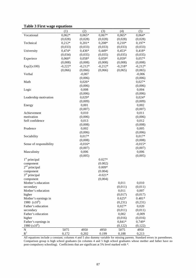
87

Table 3 First wage equations(1) (2) (3) (4) (5)

Vocational 0,062*(0,028)

0,065*(0,028)

0,067*(0,028)

0,065*(0,028)

0,064*(0,028)

Technical 0,212*(0,033)

0,201*(0,033)

0,208*(0,033)

0,210*(0,033)

0,197*(0,033)

University 0,474*(0,034)

0,436*(0,035)

0,449*(0,035)

0,453*(0,035)

0,418*(0,035)

Experiece 0,060*(0,008)

0,058*(0,008)

0,059*(0,008)

0,059*(0,008)

0,057*(0,008)

Exp2(x100) -0,222*(0,066)

-0,212*(0,066)

-0,212*(0,066)

-0,218*(0,065)

-0,212*(0,065)

Verbal -0,007(0,006)

-0,006(0,006)

Math 0,026*(0,006)

0,027*(0,006)

Logic 0,008(0,006)

0,004(0,006)

Leadership motivation 0,029*(0,009)

0,024*(0,009)

Energy 0,001(0,007)

0,002(0,007)

Achievementmotivation

0,010(0,006)

0,011(0,006)

Self confidence 0,013(0,008)

0,012(0,008)

Prudence 0,002(0,006)

0,005(0,006)

Sociability 0,017*(0,008)

0,017*(0,008)

Sense of responsibility -0,016*(0,007)

-0,015*(0,007)

Masculinity 0,006(0,005)

0,006(0,005)

1st principalcomponent

0.027*(0.002)

2nd principalcomponent

0.009*(0.004)

3rd principalcomponent

-0.021*(0,004)

Mother’s educationsecondary

0,011(0,011)

0,010(0,011)

Mother’s educationhigher

0,011(0,017)

0,007(0,017)

Mother’s earnings in1980 (x106)

0.625*(0,231)

0.481*(0,231)

Father’s educationsecondary

0,027*(0,011)

0,020(0,011)

Father’s educationhigher

0,002(0,016)

-0,009(0,016)

Father’s earnings in1980 (x106)

0,841*(0,122)

0,749*(0,122)

N 5075 4950 4950 5075 4950R2 0,172 0,202 0.199 0,188 0,213All equations include a constant; columns 4 and 5 also dummy variable for missing parents. Standard errors in parentheses.Comparison group is high school graduates (in columns 4 and 5 high school graduates whose mother and father have nopost-compulsory schooling). Coefficients that are significant at 5% level marked with *.

88

The first principal component (general ability) has a clear positive impact on earnings. Also

the coefficient of the second component (academic skills) is statistically significant and

positive. In contrast, the third principal component appears to have a negative sign. This

result is probably best interpreted by noting that the third component is negatively loaded on

''leadership motivation'' and ''sociability'' measures both of which have a positive effect on

earnings.

In columns 4 and 5, measures of parents’ education and earnings were added to the equation.

Parents' education was described with dummy variables for secondary and higher education

and an indicator for missing information. The comparison group is parents with only

compulsory schooling. The results indicate that both mother's and father's earnings have a

positive effect of son's earnings but parents' education or even missing parent does not have

any effect.

In Table 4, the same regression equations were estimated separately by the level of schooling.

Again parents' education did not have any significant effects and the table reports the results

from a specification with family background variables omitted. For brevity, only regressions

on the first three principal components are reported; below each column the test scores that

were statistically significant at the 5% level in a regression of earnings on separate scores are

listed. The first notable feature in this exercise were that the test scores explain relatively little

of the within education level variation in earnings. The R2 is greatest 0.13 for university

graduates, but just regressing their earnings on a quadratic function of experience results in an

R2 of 0.10. The first principal component is significant and positive in all education levels.

The coefficient on the second is only significant on technical schooling group. Also, the

coefficients do not vary a lot across schooling levels, suggesting that the skill prices in the

different levels of schooling may not be that different after all.

89

Table 4 Wage regressions by the level of schoolingHigh school Vocational Technical University

Experience -0,344(0,630)

0,035*(-0,017)

0,031*(0,015)

0,056*(0,016)

Exp2(x100) 1,489(2,555)

-0,107(0,125)

0,0810,143

-0,045(0,182)

1st principalcomponent

0,023*(0,007)

0,029*(0,004)

0,021*(0,004)

0,030*(0,005)

2nd principalcomponent

0,013(0,011)

0,011(0,006)

0,014*(0,007)

-0,001(0,001)

3rd principalcomponent

-0,005(0,013)

-0,018*(0,007)

-0,033*(0,008

-0,024*(0,008)

N 1456 1739 1198 1430R2 0,098 0,050 0,102 0,133Significant in a Logic Math Math Mathseparate Leadership Leadership Sociabilityregression Masculinity

4.4.3 Schooling choiceTable 5 presents estimates of the OGEV-model for schooling choice. The model is identified

by setting the coefficients for the base category (high school) equal to zero. The estimates

reported in the table are, therefore, effects of a change in the explanatory variables on the log

odds of choosing category s rather than the base category. Since the choice of the base

category is arbitrary, a proper test of the effect of a variable on the choice probabilities is a χ2-

test of the hypothesis that all coefficients corresponding to the same variable are zero across

equations. This is reported in the last column.

90

Table 5 OGEV model for schooling choice

Vocational Technical University χ2 (3)Constant 1.20 0.86 0.25Verbal -0.02 -0.11 0.10 7.26*Math -0.04 0.21 0.56 77.88**Logic -0.02 0.16 0.04 6.86*Leadership motivation -0.09 -0.24 -0.03 4.81Energy 0.09 0.14 -0.18 14.97**Achievement mot. -0.02 0.08 0.41 41.50**Self confidence -0.11 0.02 0.31 25.77**Prudence 0.11 0.25 0.35 32.60**Sociability 0.05 -0.06 -0.22 15.56**Sense of responsibility 0.10 0.11 0.13 4.29Masculinity 0.10 0.09 -0.16 23.31**No mother present -0.47 -0.36 0.02 4.78Mother’s educationsecondary

0.12 0.23 0.30 9.35**

Mother’s education higher 0.29 0.44 0.94 30.40**Mother’s earnings in 1980 -2.62 -4.50 -0.04 4.33No father present -0.32 -0.44 -0.32 5.34Father’s educationsecondary

-0.15 -0.03 0.08 5.67

Father’s education higher -0.01 0.25 0.62 24.47**Father’s earnings in 1980 -2.27 -2.83 -0.06 6.65*θ 0.17 (0.52)N 6677Pseudo R2 0.12

* significant at 10% level, χ2 (3) > 6.25;** significant at 5% level, χ2 (3) > 7.81

The coefficients for university education have the clearest interpretation. A high score in

math, achievement motivation, self-confidence and prudence measures increase the odds of

completing a university education. The odds of completing a university degree also increase if

parents have higher education. The other coefficients are not so clear cut. Some general

observations can be made. First, there are not many variables that would help predicting the

choice between quitting after high school and continuing in vocational education. Second, the

coefficients are not always proportional as would be expected if the choice probabilities were

generated from an ordered model. For example, a high score in the verbal test seems to

decrease odds of technical education and increase the odds of university education, while a

high score in the logic test has an opposite effect. Finally, correlation between the

unobservables in the adjacent categories is of reasonable magnitude, but very imprecisely

estimated. With the coefficient θ restricted to zero, the OGEV-model reduces to the

91

multinomial logit model. As shown in Small (1994), a t-test of this restriction is equivalent to

the Lagrange multiplier - specification test of the multinomial logit model against the OGEV-

model as the alternative hypothesis. Since the null hypothesis (θ = 0) is not rejected, the

multinomial logit model seems to provide a sufficient description of the choice process.

4.4.4 Selectivity corrected earnings equationsBefore estimating the selectivity corrected earnings functions two simplifications were made

to the choice model. As the estimates of the earnings functions in the previous section

suggested, the information in the test scores can be reasonably summarized in the three first

principal components. Also, based on the estimates of the choice model, the covariance

between the unobservables can be ignored, which reduces the OGEV-model to the

multinomial logit model.

For the exclusion restrictions, the available data provide two possibilities. Firstly, it can be

argued that parents' schooling has no effect on earnings. Parents’ education can still have an

impact on schooling choices either through lowering the costs of schooling or by influencing

the preferences of their son. The other possibility would be to interpret some of the

personality test scores as measures of tastes for schooling. In particular, ''achievement

motivation'' and ''prudence'' measures actually include statements of attitudes toward

schooling. Since excluding some test scores from earnings equations would make

summarizing the rest in the principal components more complicated, I chose to identify the

model by excluding parents' education.16

Table 6 presents the results from the selectivity-corrected earnings equations. Apparently, the

selectivity correction does not alter the results much and, in fact, the selectivity correction

terms are insignificant in all four estimated equations. The first principal component (general

ability) has a significant and almost equal impact in all equations. The second (academic

skills) is significant only in technical education group and the third has a negative impact in

all but the high school equation. Parents' earnings also appear important, father's earnings

have a positive and statistically significant coefficient in all equations.

16 In a specification were all the test scores entered the earnings equations separately (not shown), theresults were not sensitive for the choice of the exclusion restrictions.

92

Table 6 Selectivity corrected earnings equations

High school Vocational Technical UniversityExp -0,300

(0,629)0,035*(-0,016)

0,030*(0,015)

0,052*(0,016)

Exp2(x100) 1,302(2,555)

-0,123(0,124)

0,075(0,143)

0,004(0,182)

1st principalcomponent

0,020*(0,010)

0,021*(0,006)

0,020*(0,004)

0,024*(0,008)

2nd principalcomponent

0,013(0,013)

-0,001(0,012)

0,016*(0,007)

-0,008(0,011)

3rd principalcomponent

-0,003(0,020)

-0,019*(0,009)

-0,024*(0,009)

-0,025*(0,010)

Father’s earnings in1980 (x106)

0,915*(0,326)

0,564*(0,226)

0,744*(0,218)

0,447*(0,190)

Mother’s earningsin 1980 (x106)

-0,170(0,707)

1,230*(0,400)

-0,523(0,489)

0,321(0,351)

-φ/F -0,015(0,144)

-0,120(0,100)

-0,169(0,120)

0,044(0,091)

N 583 1739 1198 1430R2 0,038 0,063 0,116 0,144Standard errors that are corrected for the presence of generated regressors in parentheses

4.4.5 Counterfactual outcomesThe estimates in Table 6 can be used for calculating the expected earnings in each alternative

for an individual with given characteristics. The method involves simply treating the

estimated coefficients as sector specific skill prices and plugging in the observed individual

characteristics. Information on the actual choices and the estimated choice probabilities can

then be used for calculating the expected values of the error terms as described in equation

(12). A slight additional complication arises from variables, such as experience, that are

directly related to the schooling choices. In the simulations that follow all individuals are

assigned 32 years of age (median age in the sample). Then for predicting earnings at the

schooling level s, all individuals are assigned the level of experience equal to average

experience of those 32-year-olds who actually chose the schooling level s17.

17 The simulation procedure is essentially similar to that in Gregory and Vella (1996). However, theirordered probit choice model is not as attractive for simulations, because it requires an assumption that

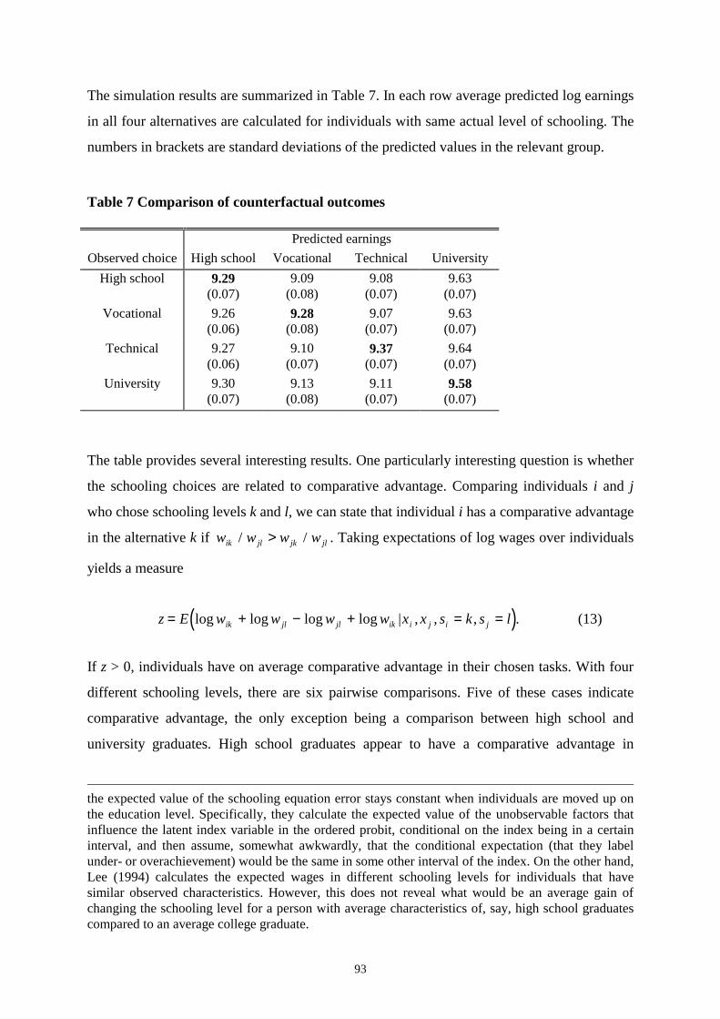
93

The simulation results are summarized in Table 7. In each row average predicted log earnings

in all four alternatives are calculated for individuals with same actual level of schooling. The

numbers in brackets are standard deviations of the predicted values in the relevant group.

Table 7 Comparison of counterfactual outcomes

Predicted earningsObserved choice High school Vocational Technical University

High school 9.29(0.07)

9.09(0.08)

9.08(0.07)

9.63(0.07)

Vocational 9.26(0.06)

9.28(0.08)

9.07(0.07)

9.63(0.07)

Technical 9.27(0.06)

9.10(0.07)

9.37(0.07)

9.64(0.07)

University 9.30(0.07)

9.13(0.08)

9.11(0.07)

9.58(0.07)

The table provides several interesting results. One particularly interesting question is whether

the schooling choices are related to comparative advantage. Comparing individuals i and j

who chose schooling levels k and l, we can state that individual i has a comparative advantage

in the alternative k if w w w wik jl jk jl/ /> . Taking expectations of log wages over individuals

yields a measure

( )z E w w w w x x s k s lik jl jl ik i j i j= + − + = =log log log log | , , , . (13)

If z > 0, individuals have on average comparative advantage in their chosen tasks. With four

different schooling levels, there are six pairwise comparisons. Five of these cases indicate

comparative advantage, the only exception being a comparison between high school and

university graduates. High school graduates appear to have a comparative advantage in

the expected value of the schooling equation error stays constant when individuals are moved up onthe education level. Specifically, they calculate the expected value of the unobservable factors thatinfluence the latent index variable in the ordered probit, conditional on the index being in a certaininterval, and then assume, somewhat awkwardly, that the conditional expectation (that they labelunder- or overachievement) would be the same in some other interval of the index. On the other hand,Lee (1994) calculates the expected wages in different schooling levels for individuals that havesimilar observed characteristics. However, this does not reveal what would be an average gain ofchanging the schooling level for a person with average characteristics of, say, high school graduatescompared to an average college graduate.

94

university education. This is not the only strange result concerning the university graduates.

According to the last column in Table 7, the individuals who ended up with a university

degree are not the ones with highest expected earnings after a university degree. This

anomality is not sensitive to changes in specification: changing the set of the excluded

variables or estimating the equations using the individual scores instead of principal

components produces qualitatively similar results. There are at least two possible

explanations. It may be that the test scores do not measure the relevant skills for university

graduates. The tests are designed to discriminate between average recruits, not necessarily

between the top percentiles that end up with a university education. Also entrance to

universities is restricted, the number of applicants being much greater than the number of

accepted students. This may break down the utility maximization assumption on which the

estimates of the selectivity corrected earnings equations and the counterfactual outcomes are

based on.

Another related observation is that Table 7 can be used for calculating returns to schooling for

particular groups. For example, the return to vocational education for those who did attend

vocational education (average effect of treatment on the treated) is the difference between

predicted earnings of individuals with vocational education minus their expected earnings had

they quit after high school. In Table 7, this corresponds to the difference between the second

and first column on the second row. Calculating returns to schooling in this manner yields

returns of 3% for vocational education, 10% for technical education and 29% for university

education. Comparable numbers for potential returns for high school students are -19%, -20%

and 34%.

95

4.5 Conclusion

It is demonstrated that several dimensions of skill are important for schooling choice and

earnings determination. The skills cannot be combined into a single dimension so that a one-

factor ability model would describe the observed variation. Of course, principal component

analysis is just one way of summarizing this data. Another option would involve selecting

some measures that could be argued to be relevant for schooling choice and earnings, for

example, mathematical and social skills and motivation. However, this choice would be

somewhat arbitrary. An attractive feature of the principal component analysis is that no a

priori assumptions on what skills might be important were needed.

Another important result is that observed skills explain relatively little of the variation in

earnings. Observing a large number of factors that would usually be in the unobservable

component increases the predictive power of the equations very little.

The schooling choices appear to be roughly consistent with the comparative advantage story.

It seems that students who did not continue in vocational or technical education had a good

reason not to do so; they actually did better with just high school education. However,

university education seems to be highly rewarded for most people. The evidence on

comparative advantage is not very strong. A basic requirement for the existence of

comparative advantage is that the rewards to skills are different in the different sectors. The

estimates of the impact of the measured skills show a surprising degree of similarity across

schooling levels.

On the econometric issues it was demonstrated that the OGEV-model can be used in

selectivity correction. However, allowing correlation between the random components of the

consecutive alternatives did not change the results. A multinomial logit model appears to be a

sufficient approximation of the choice mechanism.

96

References

Amemiya, T. (1985) ''Advanced Econometrics'', Cambridge: Harvard University Press.

Anderson, J. A. (1984) ''Regression and Ordered Categorical Variables'', Journal of the Royal

Statistical Society B 46, 1-30.

Blackburn, M. and D. Neumark (1993) ''Omitted-ability Bias and the Increase in the Return to

Schooling'', Journal of Labor Economics 11, 521-544.

Cawley, J., J. Heckman and E. Vytlacil (1998) ''Meritocracy in America: Wages Within and Across

Occupations'', NBER Working Papers 6646.

Falaris, E. (1987) Migration Model with Selectivity'', International Economic Review 28, 429-444.

Grogger, J. and E. Eide (1995) ''Changes in College Skills and the Rise in College Wage Premium'',

The Journal of Human Resources 30, 280-310.

Hay, J. (1980) ''An Analysis of Occupational Choice and Income''. Dissertation. New Haven: Yale

University.

Heckman, J. (1990) ''Varieties of selection bias'', American Economic Review, Papers and

Proceedings 80, 313-318.

Heckman, J. (1997) ''Instrumental Variables. A Study of Implicit Behavioral Assumptions Used in

Making Program Evaluations'', Journal of Human Resources 32, 441-461.

Ichimura, H. and L.F Lee (1991) ''Semiparametric Least Squares Estimation of Multiple Index

Models: Single Equation Estimation'', Chapt. 1 in W.A. Barnett, J. Powell and G. Tauchen, eds..

Nonparametric and Semiparametric Methods in Economics and Statistics, New York: Cambridge

University Press.

Lee, L.F. (1982) ''Some Approaches to the Correction of Selectivity Bias'', Review of Economic

Studies 49, 355-372.

Lee, L.F. (1983) ''Generalized Econometric Models with Selectivity'', Econometrica 51, 507- 512.

Lee, L.F. (1995a) ''The Computation of Opportunity Costs in Polychotomous Choice Models with

Selectivity'', The Review of Economics an Statistics 77, 423-435.

Lee, L.F. (1995b) ''Semiparametric Maximum Likelihood Estimation of Polychotomous and

Sequential Choice Models'', Journal of Econometrics 65, 381-428.

Maddala, G. (1983) ''Limited Dependent and Qualitative Variables in Econometrics'', Cambridge:

Cambridge University Press.

97

McFadden, D. (1981) ''Econometric Models of Probabilistic Choice'', chapt. 5 in C. Manski and D.

McFadden eds. Structural Analysis of Discrete Data with Econometric Applications. Cambridge:

MIT Press.

Murnane, R., J. Willet and F. Levy (1995) ''The Growing Importance of Cognitive Skills in Wage

Determination'', The Review of Economics and Statistics 77, 251-266.

Roy, A. (1951) ''Some Thoughts on the Distribution of Earnings'', Oxford Economic Papers 3, 135-

146.

Schmertmann, C. (1994) ''Selectivity Bias Correction Methods in Polychotomous Sample Selection

Models'', Journal of Econometrics 60, 101-132.

Small, K. (1987) ''A Discrete Choice Model for Ordered Alternatives'', Econometrica 55, 409-424.

Small, K. (1994) ''Approximate Generalized Extreme Value Models of Discrete Choice'', Journal of

Econometrics 62, 351-382.

Trost, R. and L.F. Lee (1984) ''Technical Training and Earnings: A Polychotomous Choice Model

with Selectivity'', The Review of Economics and Statistics 66, 151-156.

Vella, F. and R. Gregory (1996) ''Selection Bias and Human Capital Investment: Estimating the Rates

of Return to Education for Young Males'', Labor Economics 3, 197-219.

Vella, F. (1998) ''Estimating Models with Sample Selection Bias: A Survey'', Journal of Human

Resources 33, 127-169.

98

Appendix. Description of the Finnish Army basic ability test18

Part 1, Basic skills (Peruskoe 1)Each test consists of 40 multiple-choice questions. The raw score is the number of correct

answers.

Math: The test consists of simple arithmetic operations, short problems given in a verbal

form and completition number series that are arranged according to a certain rule.

Verbal: The questions involve choosing a word that is a synonym or an antonym of a given

word, selecting a word pair that displays a similar relationship than a given word pair and to

choosing which word does not belong to a given group of words.

Logical: The questions show a matrix of figures with one figure missing. The examinee has

to decide which figure completes the matrix.

Part 2, Leadership inventory (Peruskoe 2)The items are yes/no statements that sum up to the following scores.

Leadership motivation: A person with a high score is socially active and brave. He wants to

make plans, and to influence others. He also trusts in his ability to lead others and he takes a

responsibility of his actions also in difficult situations. A person with a low score rather

remains on the background and avoids situations where he would have to be responsible of

planning and leading.

Energy: A person with a high score is vital and action-oriented. He gets started quickly and

works effectively and quickly. He has to be almost constantly doing something. A person

with a low score is slow and phlegmatic and avoids physical action. He expects that problems

solve themselves. Tasks that require speed or constant action are stressful for him.

Achievement motivation: A person with a high score enjoys studying. He sets his goals high.

Achievement is important for him and he is confident that he will be successful. A person

18 Translated and shortened from unpublished Finnish Army documents.

99

with a low score has a negative attitude towards schooling. He does not have high goals and

he puts minimum effort in his work.

Self-confidence: A person with a high score believes in himself. He views himself at least as

able and intelligent than others and believes that he will manage in life, if necessary, even

without help from others. A person with a low score is uncertain about himself. He gives up

easily and blames others for his failures.

Prudence: A person with a high score plans far in the future and considers carefully the

results of his actions. He avoids taking unnecessary risks. A person with a low score is

impulsive and cannot resist temptations. He gets excited easily but has a careless attitude, and

often fails to finish his tasks.

Sociability: A person with a high score seeks company of other people. He enjoys talking and

entertaining others. He finds it easy to meet new people and to create new relationships. A

person with a low score is quiet and reserved. He has trouble to express himself and he is

afraid of public presentations.

Sense of responsibility: A person with a high score has high ethical and moral standards. He

is usually trustworthy and takes the responsibility if things go wrong. A person with a low

score avoids taking personal responsibility. He has rather loose ethical and moral standards

and a tendency to act against commonly accepted norms.

Masculinity: A person with a high score prefers traditionally male dominated occupations.

He also prefers action and excitement to emotionally sensitive thinking. A person with a low

score is an emotional person. He is intellectually and culturally oriented and prefers female

dominated occupations.

100

Chapter 5

Trends in between- and within-group

earnings inequality in Finland

Abstract

This study describes the changes in the wage structure in Finland between 1977 and1995, and provides a simple explanation based on demand and supply of skills. Thestudy augments the single index model of Card and Lemieux (1996) to incorporatechanges in the supply of skills. The augmented model adequately accounts for thechanges in the relative wages between groups of different education and experience,but does not capture the changes in within-group distribution.

Keywords: Wage dispersion, return to skill

5.1 Introduction

Studies of trends in the wage distribution typically decompose changes in inequality into

changes in earnings differences between some skill groups (for example levels of education)

and changes in dispersion within these groups. While changes in between-group inequality

can often be reasonably well explained in a simple supply-demand framework, changes in

within-group distribution do not fit as well into the standard Economics 1 analysis. In this

paper, I present a simple conceptual framework for analyzing both between- and within-group

changes in inequality. I also test the hypotheses implied by the model using data from the

Finnish Income Distribution Surveys 1977-1995.

101

The revival of interest in earnings inequality among economists was largely caused by the

dramatic increase in the earnings differences in the US during the 1980's (e.g. survey by Levy

and Murnane, 1992). The US experience was shared to a lesser extent by other OECD

countries, particularly the UK (Gottshalk and Smeeding, 1997). Changes in the wage

distribution in Finland have been smaller than in the US or the UK. However, Eriksson and

Jäntti (1997) report a substantial increase in inequality between 1985 and 1990. They also

find that the change was mostly due to increasing wage dispersion within groups of workers

with similar education and experience.

Several explanations for the increase in earnings inequality have been proposed in the

literature. Changes in the institutional setting, such as the decline in the real value of the

minimum wage and the decline in unionization, may have increased the dispersion of

earnings. The greatest increase in inequality occurred in the countries with least centralized

wage bargaining, US and UK (Gottschalk and Smeeding 1997). Decentralization may also

help explaining the developments in other OECD countries, since even in countries where the

unionization rates remained high, there was a movement toward more decentralized wage

bargaining (OECD Employment Outlook 1993).

Supply-related reasons, such as changes in the quantity (or quality) of labor supply across

skill groups, were advocated, for example, by Katz and Murphy (1992) and, using Swedish

data, by Edin and Holmlund (1995). In a world where workers with different educational

qualifications are imperfect substitutes in production, an increase in the relative size of a

group will decrease the relative wage of that group (and vice versa). However, in most

countries the proportion of the workforce with higher levels of education grew simultaneously

with the relative earnings of highly educated workers. Therefore, it is clear that changes in

relative supplies are not sufficient to explain the observed changes in the relative wages, but

some demand side explanations are required as well.

The demand side explanations for widening inequality include the decline in manufacturing

employment, maybe partly caused by an increase of international trade. Other explanations

relate changes in the relative demand of different types of workers to changes in final product

demand, such as increased demand for services. It has been argued that the flow of less

educated workers from the highly paid manufacturing jobs to the low productivity service

jobs increased wage inequality. However, since wage differences have increased also within

102

industries, even this cannot be a sufficient explanation. An emerging consensus view of the

demand side factors emphasizes the role of skill-biased technological change. Advanced

technology and skilled labor appear to be complements in production and technological

change increases the relative productivity of the more skilled workers. The empirical problem

in assessing the merits of this theory is that the rate of technological change and its effect on

relative labor demand is hard to measure. Technological change is often the residual factor

that is used to explain the changes that cannot be accounted for by the observed factors. Some

direct evidence on this issue is provided by the studies that show how, for example, the

spread of computing technology has changed the wage structure (Krueger, 1993).

In this paper, I use changes in wage dispersion within narrowly defined age/education groups

to identify demand effects. I therefore assume that variability in wages within groups of

employees with similar education and experience is partially caused by differences in skills

not captured with these human capital proxies. If technological changes cause more skilled

workers to become relatively more productive, we would expect an increase in both between-

group and within-group wage inequality. However, provided that the within-group skill

distribution stays approximately constant, the relative supply changes should only affect

between group variation.

The rest of this article is organized following the suggestion by Levy and Murnane (1992).

They present three questions that an ideal study on earnings inequality trends should answer,

namely:

1. What is the trend in earnings inequality over the period under study?

2. Along what dimensions is inequality changing?

3. What shifts in demand, shifts in supply and/or changes in wage setting institutions are

responsible for the observed trend?

I thus begin by documenting the changes in the earnings distribution in Finland during the

period from 1977 to 1995 trying to answer the first two questions in section 5.2. The

conceptual framework for answering the most difficult third question is formulated in section

5.3. Section 5.4 presents the empirical results and section 5.5 presents some concluding

comments.

103

5.2 Recent trends in the distribution of earnings in Finland

Contrary to popular belief, the wage distribution in Finland is not particularly compressed.

Nor are the returns to observed skills, such as schooling, low in international comparison.

According to the figures published in the OECD Employment Outlook (1996), the earnings

dispersion among full-time full-year workers in Finland in 1991 was roughly in the level with

Germany and Italy and clearly higher than in the other Nordic countries. Also, another OECD

study shows that in 1992, the earnings difference between men with university education and

with only upper secondary education, was the highest among the OECD countries in Finland.

For women, this difference was third highest in the OECD (OECD, Education at Glance

1995)1.

Previous studies on the trends in the earnings inequality in Finland present somewhat mixed

results. Using data from manufacturing industries, Asplund (1994) finds only very small

changes in the overall wage dispersion between 1980-1992. The wage dispersion declined

slightly in the beginning of the 1980's, increased slightly up to the turn of the decade and

started a new decline in the early 1990’s. However, Asplund finds a large decrease in the

return to education between 1980 and 1985 for the white-collar employees. (She had no data

on the education of blue-collar employees.) OECD Employment Outlook (1996) that uses

data from the Income Distribution Survey, shows a similar pattern. Income dispersion appears

to have declined in the end of 1970's and started a slow increase in 1980. Inequality peaked in

1989 and declined slowly after that. The changes have, however, been much more modest

than in Canada, US and UK. Results by Eriksson and Jäntti (1997) are quite different. Using

data from quinquennial population censuses 1971- 1990, they find a sharp increase in

earnings inequality between 1985 and 1990. They note that this increase, which followed a

steady decline in inequality, was comparable in magnitude to increases observed in the United

States and the United Kingdom. In their decomposition of the changes of earnings dispersion,

they find that the 1970's decrease in inequality can be accounted for by changes in observed

characteristics and changes in returns to these characteristics, but that the increase in

inequality between 1985 and 1990 occurs almost completely in the within-group dispersion.

1 It should be noted that due to high tax progression and generous transfer programs, the post-taxincome differences in Finland are much smaller. In fact, a recent cross-country study by Atkinsson,Smeeding and Rainwater (1995) shows that Finland had the most equal distribution of householddisposable income among the OECD countries in their sutdy.

104

I start this section by describing trends in the dispersion of earnings based on published data

from the Finnish Income Distribution Survey. After that I present more detailed results based

on microdata for the years 1977, 1983, 1989 and 1995 of the same survey.

The Finnish Income Distribution Survey produces annual data on the level, formation and

distribution of incomes among households. The main income concept is disposable income,

but the survey also gathers data on the taxable earnings of individuals who belong to the labor

force. It was first conducted in 1977 and since 1983, it has used a rotating panel design where

each household is interviewed in two consecutive years and approximately half of the old

panel is replaced with a new sample every year. The survey uses stratified sampling and

oversamples high income households. The primary sampling unit is the household and all the

members of the household are included in the data. The microdata includes weights based on

sampling probabilities. These weights are calibrated to match population distribution in

income and various household characteristics. The sample size has varied from 46,600

households and 100,821 individuals in 1977 to 9,262 households and 25,229 individuals in

1995. The information in later years is based mostly on administrative registers, interviews

are used for some classification information and for some income sources that are not

available in registers. Most importantly for the present study, the earnings information is

based on tax records that should be highly reliable.

5.2.1 Trends in aggregate time seriesEvolution of real earnings

The period from 1977 to 1990 was characterized by strong economic growth. In 1977, the

Finnish economy was in recession. The recovery started in 1978 and stable growth continued

during the 1980's. An average annual growth rate of the real earnings of the median worker

was almost 2.5% between 1977 and 1990. Turnaround in the stable growth came with the

economic crisis in 1990. Average real earnings declined for several years and were in 1995

almost at the level of 1990. Figure 1 shows the development of real annual earnings of wage

earners by deciles based on the published figures of the Income Distribution Survey. For

comparability over time, the figures include all wage earners, therefore combining part-time

and full-time workers as well as workers who have been employed only part of the year.

Obviously this causes a problem when comparing periods with high and low unemployment

rates.

105

Figure 1. Annual real earnings by decile in 1990 marks.Note: Data includes all wage earners.Source: The Income Distribution Survey. The Survey was not conducted in 1981 nor 1985.

Aggregate measures of inequality

Dispersion of earnings among full-time workers has increased for both men and women from

1980 to 1989. Since the gap between men and women simultaneously decreased, the rise in

inequality among all employees was less than among men and women separately. Among

women the top decile gained compared to the median, whereas among men the widening of

earnings distribution occurred both in the 90/50 ratio and in the 50/10 ratio. After 1989 the

earnings dispersion declined sharply. Since figures are based on data on full-time year-round

workers, this decline was probably partly caused by the relative increase in unemployment

among low earners.

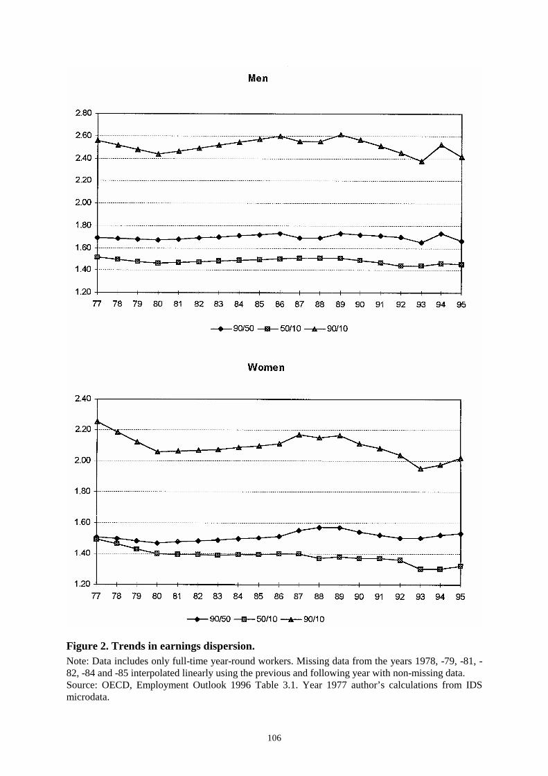
106

Figure 2. Trends in earnings dispersion.Note: Data includes only full-time year-round workers. Missing data from the years 1978, -79, -81, -82, -84 and -85 interpolated linearly using the previous and following year with non-missing data.Source: OECD, Employment Outlook 1996 Table 3.1. Year 1977 author’s calculations from IDSmicrodata.

107

Trends in the return to education

Earnings differences between different educational categories continued their decrease that

had started earlier in 1970's (Eriksson and Jäntti, 1997). Some leveling of the trend, and even

a partial rebound in returns to education can be seen in between 1985 and 1990 but the

decline of relative wages of more educated employees seems to have continued during the

1990's recession. The 1990's development is again problematic: an increase of unemployment

was more severe for workers with less education. However, it is not clear whether this

increased or decreased the wage differences among the employed workers.

Besides the trends, also the levels of relative earnings are of interest. Due to the classification

used by Statistics Finland, a college - high school wage differential, often used in

international comparisons, cannot be calculated from these data.2 Here a more natural

comparison is the earnings premium of various education categories compared to employees

with only the compulsory nine years of education. On average, during the period under the

study, men with university education have earned approximately twice as much as men with

only compulsory education. For women the difference has been approximately 80%.

Interestingly, lower secondary education (two years of vocational schooling) seems to bring

no wage gain. In several years, the average earnings of employees with lower secondary

schooling have been less than the average earnings of employees with only compulsory

schooling3.

2 High school graduates are classified as having ''upper secondary education''. However, in the 1995census only slightly over 40% of all persons classified into this group had a high school diploma asthe highest degree. The rest had completed some vocational upper secondary level education (SVT1997).3 This is partly explained by differences in work experience. The share of workers with onlycompulsory schooling is higher in the older cohorts.

108

Figure 3. Annual earnings of employees by the level of education compared to earningsof employees with compulsory level education.Source: The Income Distribution Survey. Data includes both part time and full time workers.

109

Trends in the supply of skills into labor market

Educational attainment of new labor market entrants has risen quickly. As the new entrants

replace the older, less educated workers, the average education level of the labor force

increases, though more slowly than the average education level of the new entrants.

Therefore, education is rather unequally distributed across the age groups. In 1995, 25-34 year

old Finns had a higher average education level than those in the same age group in other

Northern-European countries, but 55-64 old Finns had much less education than their

Northern-European counterparts. (OECD Education at Glance 1995).

Figures 4a and 4b show the trends in the levels of education among wage earners between

1977 and 1995. Clearly, for both men and women the number of workers with only

compulsory education has steadily declined. It appears that the share of lower secondary

education first increased but started to decline as the share of those with upper secondary

schooling increased. Although the number of employees with higher education has grown

more than 50% for men and almost 90% for women, their share of all employees, even at the

end of the period, was only about 20% .

110

Figure 4. Wage earners by the level of education.Source: The Income Distribution Survey. Missing data from years 1981 and -85, when the Surveywas not conducted, replaced by the average of previous and following years.

111

Trends in industry composition of the labor force

The composition of employment by industry has also changed rapidly in Finland. In 1970, a

quarter of the workforce was still involved in primary production. By 1995, the share of

primary production had declined to 8%. Employment in the service sector has increased fairly

steadily since 1970 reaching 65% of all workers in 1995. Since the service sector employs

women and employees with higher education in larger proportion, the increase of demand for

services benefits these groups. As a matter of fact, the service sector has largely absorbed the

increase in the labor force, caused by an increase in women's labor force participation rate.

Interestingly, manufacturing and construction maintained their share of employment until the

economic downturn in the beginning of 1990's. In fact, the absolute levels of employment in

both manufacturing and construction were almost identical in 1970 and in 1990. The largest

change in the industrial structure occurred in the 1990's when the economic crisis wiped away

some 200,000 manufacturing and construction jobs.

Figure 5 Employment by industry.Note: Classification based on SIC 1979, after 1990 on SIC 1988. Change in classification correctedby adjusting the figures after 1990 using the ratio of workers in each category according to SIC 1988and SIC 1978 in the year 1989 when both figures were available.Source: Labor Force Surveys 1970-1995.

112

5.2.2 Evidence from microdataAggregate figures of the wage distribution mask some important developments in the wage

structure. For example, a general increase in women's wages and labor force participation

rates has a big impact on aggregate wage distributions. Even more seriously, the changes in

unemployment make figures based on annual earnings hard to interpret. Microdata offers an

opportunity to control for these changes, at least to some extent, and to focus on earnings

measures that are more closely linked to the productivity differences.

In order to analyze the main components of the changes in the wage distribution, I estimated

several simple cross-section earnings equations. In each available survey year, log monthly

earnings were regressed on a set of dummy variables for six post-compulsory education

levels, a quadratic function of age, 12 regional dummies and 9 industry dummies. Estimates

are presented in Appendix 1. The estimates show a clear decrease in the return to education

between 1977 and 1983. For example, the relative earnings of Master's degree holders

compared to those with only compulsory education decreased by about 6 percentage points

for both men and women. General compression of education related wage differentials was

fairly similar across all education categories. Returns to education increased again between

1983 and 1989, but did not quite reach the 1977 level. During the recession of the 1990's the

returns to education decreased. However, employment shares changed drastically during the

recession - employment of the less educated fell much more between 1989 and 1995.

Therefore, taking into account the employment prospects would result in a more positive

impression of the change in the value of education. Interestingly, return to the work

experience (proxied by age) behaved quite differently over the period under the study,

remaining approximately constant. An inspection of the residual variation reveals that

variation in earnings not accounted for by the variables in the model, follows a pattern similar

to the that of the return to education. RMSE decreased slightly between 1977 and 1983,

increased up to 1989 and decreased again between 1989 and 1995.

In Table 1, I used data from the Income Distribution Survey to calculate various measures of

the earnings dispersion. The table shows 90/10, 50/10 and 90/50 decile ratios and the variance

of log earnings. Aggregate wage differentials appear to have decreased between 1977 and

1983, though examining men and women separately gives mixed results. Bigger changes

occured after 1983. Development from 1983 to 1989 and from 1989 to 1995 has also been

more uniform with wage inequality increasing in the former period and decreasing in the

113

latter. Movements in the 90/50 ratio appear to have been slightly bigger, than movements in

the 50/10 ratio.

Table 1. Inequality measures77 83 89 95

AllVariance of logarithms 0.161 0.153 0.163 0.138Decile ratio 90/10 0.959 0.920 0.967 0.892

50/10 0.447 0.403 0.419 0.39290/50 0.512 0.517 0.548 0.500Male

Variance of logarithms 0.152 0.156 0.173 0.152Decile ratio 90/10 0.909 0.937 1.012 0.939

50/10 0.402 0.411 0.446 0.43290/50 0.507 0.526 0.566 0.507Female

Variance of logarithms 0.111 0.106 0.118 0.100Decile ratio 90/10 0.797 0.762 0.821 0.767

50/10 0.382 0.348 0.360 0.33390/50 0.415 0.414 0.461 0.434

Note: Decile ratios are approximated by differences in log wages. For data definitions, see appendix.

In Table 2, I decompose changes in log variance to changes in the observed and the

unobserved components. The total change in the variance is simply the difference between

variance in log wages in the consecutive surveys, while the unobserved change is the change

in the variance of residuals from the regression in Appendix 1. This decomposition shows

that the increase in the earnings variance between 1983 and 1989, as well as the decrease

between 1989 and 1995, is mainly due to change in the unobserved components.4 A small

increase in dispersion in men's earnings between 1977 and 1983 appears to be accounted for

by the regressors but an equally small decrease in dispersion in women's earnings during the

same period is not.

4Calculations based on the census data in Eriksson and Jäntti (1997) are qualitatively similar but theyreported much bigger changes than what is found here. A partial explanation for the difference is thatEriksson and Jäntti used data on annual earnings. Their figures are influenced by the variation inmonths worked that may account for a large fraction of the variation in annual earnings. However,their main finding of an increase in the within-group inequality in the late 1980's is reproduced hereeven though the endpoints of the investigated period differ.

114

Table 2 Change in the variance of log earnings83-77 89-83 95-89

AllTotal -0.008 0.010 -0.025Observed -0.005 0.000 -0.011Unobserved -0.003 0.010 -0.014MaleTotal 0.004 0.017 -0.021Observed 0.006 -0.003 -0.002Unobserved -0.002 0.020 -0.019FemaleTotal -0.005 0.012 -0.018Observed -0.001 0.006 -0.004Unobserved -0.004 0.006 -0.014

Note: Unobserved change refers to change in the variance of residuals in the regression in Appendix 1of log mothly earnings on 7 education levels, age, age squared, 9 indusry and 12 region dummies.Observed change is the difference between change in the total variance and the change in the errorvariance.

To complete this section on recent trends in wage inequality, I calculated the returns to

schooling by cohort and survey year. If supply changes play a role in changes in the return to

schooling we might expect younger cohorts to have smaller returns to education. The question

is, of course, impossible to answer because age, time and cohort effects can not be separately

identified, even in a panel setting. Knowing any two will determine the third. Such analysis is

still not useless and may detect some patterns in data. In Table 3 one follows a cohort over

time by moving horizontally across columns in the same row. Changes within a cohort are

due to age or time effects. One follows the same experience group over time by moving

upward along a diagonal. Changes along this dimension are due to cohort or time effects.

Looking at figures in the same column is equivalent to estimates in a single cross section by

age group. For example, the top left corner shows return to schooling for those born between

1949 and 1954 in 1977 when they are 23 to 28 years old. The next figure to the right shows

their return to schooling in 1983 when the cohort is between 29 and 34 years of age.

115

Table 3a. Returns to schooling by cohort and year, menBirth cohort 1977 1983 1989 19951967-72 .0333

1961-66 .0507 .0534

1955-60 .0554 .0723 .0902

1949-54 .0514 .0703 .0874 .0760

1943-48 .0750 .0877 .0971 .0964

1937-42 .0952 .0994 .1082 .0854

1931-36 .1093 .1047 .1143 .0949

1925-30 .1314 .1117 .1137

1919-24 .1214 .1129

1913-18 .1180

Table 3b. Returns to schooling by cohort and year, womenBirth cohort 1977 1983 1989 19951967-72 .0472

1961-66 .0639 .0699

1955-60 .0575 .0780 .0790

1949-54 .0594 .0786 .0804 .0807

1943-48 .0774 .0763 .0844 .0800

1937-42 .0865 .0840 .0795 .0728

1931-36 .0936 .0912 .1058 .0753

1925-30 .0903 .0719 .0868

1919-24 .0853 .0931

1913-18 .0953

Note: The figures in graph are coefficients on years of schooling in a cross-section regression by agegroup. Sampling weights are used in estimation. All equations include 12 region and 9 industrydummies. Data as in Appendix 1, but years of schooling are calculated from the highest degreeachieved according to the Statistics Finland education classification.

Two observations are fairly clear. Firstly, youngest workers have the lowest returns to

schooling. The top figure in each column is the smallest and this does not appear to be a

cohort nor a time effect. Secondly, the returns to schooling appear to be lowest in 1995 no

matter whether the cohort or the age is held constant.5 For the rest of the table it is much

harder to detect obvious patterns. Since the figures seem to change more by the rows (cohort

constant) and by the columns (year constant) than by the diagonal (age constant), it seems that

the age effects are dominating. Of course, the same pattern could be caused by an interaction

of the cohort and the time effects.

5Standard errors of the estimates vary because the sample size varies by year and age group, but 95%confidence intervals are in most cases around [b-0.01,b+0.01].

116

In the next section I try to provide an explanation for the observed changes but at this point a

short summary of stylized facts might be useful.

During the period from 1977 to 1989, Finland underwent a fairly smooth transition in

industrial structure with a shift of workers from primary production to services. At the same

time, the share of more educated labor steadily increased. Movements in the wage structure

were modest. Returns to the education had a negative trend, though this trend was somewhat

reversed in the late eighties. Simultaneously with the rebound of the return to education,

unexplained variation in earnings clearly increased. Economic crisis in the 1990's caused

quite dramatic changes. Unemployment rates rose for all workers, but the employment losses

were much bigger for the less educated. For those who remained at work, real earnings

growth ceased and wage dispersion decreased in all dimensions.

5.3 Explanations for the observed changes

A coherent explanation of the changes in the wage distribution should be able to account for

changes in both between-group and within-group differences. As noted above, the first task is

considerably easier than the second. Understanding changes in the within-group wage

dispersion requires some idea of what are the causes of wage differences between workers

with similar education and work experience. No doubt, much of this variation is simply

random; for some reason wages do not equal productivitities. Part of the observed wage

dispersion is just measurement errors in earnings or hours that is always likely to be present in

any data. Some fraction of the within-group dispersion could be explained by industry wage

differences and increasing the number of covariates in the wage equations would make the

within-group dispersion smaller. However, it is questionable whether these factors could

explain the changes in the within-group dispersion. But, if within-group wage differences

reflect differences in skills that are valued by employers but not observed in the data, changes

in the within-group wage dispersion could be explained by changes in demand for those skills

(Katz and Murphy 1992, Juhn Murphy and Pierce 1993).

There is not very much evidence on what these unobservable skills that are in growing

demand would be. Results obtained by Blackburn and Neumark (1991) and Bishop (1994)

suggest that skills measured by standardized tests do not explain a very large fraction of the

117

within-group wage dispersion. Bell (1996) shows that computing skills became more valuable

during the 1980's but even in his regressions, the residual variation did not decrease much

after adding an indicator of a computer use. Results on the Finnish data are rather similar both

in terms of the predictive power of test scores (Uusitalo 1996) and computer use (Asplund

1997)6.

The best proxy for skills available in commonly used datasets is educational attainment. One

might expect that if the within-group dispersion is caused by the unobservable skills,

increases in the within-group dispersion would coincide with increases in the return to

education. As shown in the previous section, this prediction is roughly consistent with the

observed development in Finland. However, if workers with different educational

qualifications are imperfect substitutes in production, returns to education are also influenced

by changes in relative supplies. Below, I formulate a model that incorporates both changes in

the demand for skills and changes in the supply.

5.3.1 Single-skill modelA simple explanation for the observed changes in the between- and within-group inequality

was proposed by Card and Lemieux (1996). They formulate a single-index model relating the

relative wages to a one dimensional skill index. In their model, a generic increase of the

relative productivity of the more highly skilled workers is expected to increase the wage

differentials between age and education groups as well as to raise wage inequality within

narrowly defined age/education cells. The first part of this section outlines the basic structure

of the Card - Lemieux model and restates its empirical implications. The second part extends

the model to incorporate supply effects.

First assume a single-index model, where the wage equals the value of the marginal product.

This could be the case if the production technology were such that all workers were perfect

substitutes. In period t output Yt is produced using labor inputs from M groups with Nht

workers in each group. The relative productivity of workers in group h in period t equals θht

( )Y f Nt ht hth

M

=

=

∑ exp θ1

(1)

6Asplund (1997) also finds that the wage premia for computer use disappeared between 1991 and 1993.

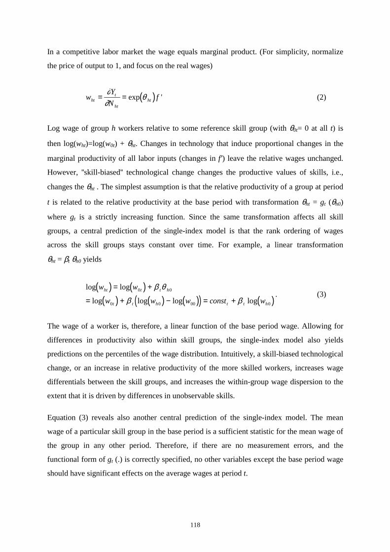
118

In a competitive labor market the wage equals marginal product. (For simplicity, normalize

the price of output to 1, and focus on the real wages)

( )wY

Nfht

t

htht= =

∂∂

θexp ' (2)

Log wage of group h workers relative to some reference skill group (with θ0t= 0 at all t) is

then log(wht)=log(w0t) + θht. Changes in technology that induce proportional changes in the

marginal productivity of all labor inputs (changes in f') leave the relative wages unchanged.

However, ''skill-biased'' technological change changes the productive values of skills, i.e.,

changes the θht . The simplest assumption is that the relative productivity of a group at period

t is related to the relative productivity at the base period with transformation θht = gt (θh0)

where gt is a strictly increasing function. Since the same transformation affects all skill

groups, a central prediction of the single-index model is that the rank ordering of wages

across the skill groups stays constant over time. For example, a linear transformation

θht = βt θh0 yields

( ) ( )( ) ( ) ( )( ) ( )

log log

log log log log

w w

w w w const wht t t h

t t h t t h

= +

= + − = +0 0

0 0 00 0

β θ

β β. (3)

The wage of a worker is, therefore, a linear function of the base period wage. Allowing for

differences in productivity also within skill groups, the single-index model also yields

predictions on the percentiles of the wage distribution. Intuitively, a skill-biased technological

change, or an increase in relative productivity of the more skilled workers, increases wage

differentials between the skill groups, and increases the within-group wage dispersion to the

extent that it is driven by differences in unobservable skills.

Equation (3) reveals also another central prediction of the single-index model. The mean

wage of a particular skill group in the base period is a sufficient statistic for the mean wage of

the group in any other period. Therefore, if there are no measurement errors, and the

functional form of gt (.) is correctly specified, no other variables except the base period wage

should have significant effects on the average wages at period t.

119

5.3.2 Application for cell means and quantilesA single individual is not likely to be observed in several years in repeated cross section data.

Even in panel data, an individual does not belong to the same education/experience group in

the different years. However, if the within-group skill distribution stays constant, the model

yields empirically testable implications in cell means and quantiles.

Card and Lemieux (1996) assume that observed log wage of an individual i in the cell h at the

period t consists of the average productivity of the individuals in cell θ ht , the individual

deviation from the group mean aiht iht ht= −θ θ , which reflects unobserved individual specific

productivity factors, and random errors εiht, which reflect measurement errors, labor market

errors etc.

( )log w aiht ht iht iht= + +θ ε (4)

where aiht and εiht are normally distributed with zero means variances σ a2 and σ ε

2 The mean

log wage of workers in group h in the base period is therefore

( ) [ ]log w E ah h ih ih h0 0 0 0 0= + + =θ ε θ , (5)

and given that the transformation of the productive value of skills is linear from year to year

θt = αt + βt θ0 the mean wage in period t is

( ) [ ] ( )log logw E a const wht t t h t ih ih t t h= + + + = +α β θ β ε β0 0 0 0 . (6)

Similar expressions can be derived for wage quantiles. Changes in the return to skill also

change the within-cell wage distribution if a fraction of within-cell variance in wages is

attributed to differences in unobservable skills. The qth quantile of wages in the cell h is

( ) ( )log w z s ahtq

htq

iht iht= + ⋅ +θ ε (7)

where zq denotes the qth percentile of the standard normal distribution and s(.) is the standard

deviation of within-cell wage distribution. Applying a linear transformation on both

120

observable and unobservable skill components yields an expression that relates wage

quantiles on the corresponding quantiles in the base year.

( ) ( )( )

log

log

w z s a

const w s z

htq

t hq

t ih iht

t t hq

hq

h

= + + ⋅ +

= + + ⋅ ⋅

α β θ β ε

β δ0 0

0

(8)

where

( )( )( )

s

R R

R

h a

h t h h t

h a

2 2 2

2 1 2

2 2 2

1

= +

= − + −

= +

σ σ

δ β β

σ σ σ

ε

ε ε

/

/

The equation (8) can be estimated by regressing wages of the qth percentile of skill groups in

the year t on constant, previous period wage and quantile-specific intercepts. If the within-

group wage dispersion is driven by changes in the relative demand for skills, the coefficients

of the base period wages should be equal across different quantiles. Furthermore, if the return

to skill has increased (β > 1) and if a part of the within-cell variance is measurement error (R

> 0), the expression for δh is negative. Therefore, we would expect the wages of lower

quantiles to grow by more and upper quantiles by less than the median.

5.3.3 The effect of supply changesIn order to incorporate changes in the relative supply of different skill groups, a slightly more

complicated production technology must be specified. A simple assumption is a CES-

production function with M groups and Nht workers in each group, all providing labor input

Xit. Further, assume that workers are perfect substitutes within same sex-education-experience

cell but imperfectly substitutable across groups. This is a special case of the two level CES-

production function (Hamermesh 1993, p. 39, eq. 2.41).

( )Y Xt iht ihti

N

h

M ht

=

==

∑∑ exp

/

θρ ρ

11

1

(9)

121

Assuming that the relative labor supply is exogenous7, the wage of an individual i is

determined by the marginal productivity at full employment:

( )( )

( ) ( )

( )( )

wY

X

Y

ihtt

ihtX iht

i

N

h

M

ihti

N

iht

t

ihti

N iht

iht

ht ht

ht

= =

×

=

===

−

=

−

=

−

∑∑ ∑

∑

∂∂ ρ

θ ρ θ θ

θθ

ρ ρ ρ ρ

ρ

111

1

1

1

1

1

1 exp exp exp

expexp

/

.

(10)

Taking logarithms and using approximation ( )exp θ θih h hi

N Nh ==∑ 1

yields

( ) ( ) ( ) ( )[ ]log log logw Y Niht t ht ht iht= − − − +1 ρ θ θ . (11)

Mean log wages in cell h at period t are then

( ) ( ) ( ) ( )[ ]log log logw Y Nht t ht ht ht= − − − +1 ρ θ θ , (12)

and log wages of qth quantile of cell h

( ) ( ) ( ) ( )[ ] ( )log log log .w Y N z s ahtq

t ht ht htq

iht iht= − − − + + ⋅ +1 ρ θ θ ε (13)

s() denotes the standard deviation of the within-cell wage distribution. Let us suppose again

that the relative productivity is related to the relative productivity at the base period by a

linear transformation θt = αt + βt θ0. Using the expressions above, cell means and quantiles of

wages can then be written as a function of the base period wages and supply changes

( ) ( ) ( )[ ]log log log logw const w N Nht t h ht h= + − − −β ρ0 01 (14)

( ) ( ) ( )[ ]log log log logw const w N N s zhtq

t hq

ht t h hq

h= + − − − + ⋅ ⋅β ρ β δ0 01 . (15)

7This is not very far from reality in Finland were the supply of educated labour mainly depends on thenumber of slots in the government-run education system.

122

Both of the above equations are nonlinear in parameters, but with β close to one, the terms in

square brackets can be reasonably approximated with changes in log supplies.

The equations (14) and (15) are the equations to be estimated. Extending the single-skill

model to incorporate supply effects simply adds in the equations an additional cell-specific

term that reflects changes in the relative supplies. If the productive value of the skills

increases (βt > 1) and relative supplies stay constant, both the between-group wage

differences and the within-group wage dispersion increase. However, a change in relative

supply only affects between-group differences with no effects on the within-group

differences. Note also that the supply change identifies the intergroup elasticity of

substitution, σ (Hamermesh 1993):

( )− = − −1 1/ σ ρ . (16)

5.4 Empirical results

To estimate the augmented single-skill model, I first divided the data from each survey into

48 cells based on sex, six education categories8 and ten-year age-intervals9. The self-

employed and those who had worked for less than six months in the survey year were

excluded from the data. For this restricted sample, a measure of monthly wage was

constructed based on the annual taxable wage and salary income and information on the

number of months spent at paid employment, counting every month in part-time work as half

a month. The individuals whose calculated monthly earnings were less than 3000 marks in the

1995 prices were dropped. This restricted sample, weighted by the sampling weights, was

used to calculate means and quantiles of the cell wages.

In order to calculate changes in supply, fever restrictions were applied. Following Katz and

Murphy (1992), all members of the labor force were included, no matter whether they were

employees, self-employed or unemployed. A weighted sum of months in the labor force over

all individuals in the cell was used as a measure of labor supply. Normalizing the labor

8Those with postgraduate education are merged with those with Master's level education.9Groups are 25-34, 35-44, 45-54 and 55-64. The youngest (below 25) and the oldest workers (over64) are excluded.

123

supplies in the cells by dividing each by the total supply in each year resulted to a cell

employment share, a log of which was included in the estimated equations. Changes in the

supply measure are, therefore, driven by the changes in the age structure, the changes in the

labor force participation rate and the changes in the education composition of the successive

cohorts. On the other hand, changes in the demand conditions only affect this supply measure

if the changes in employment opportunities induce changes in participation.

There are some obvious problems in explaining mean cell wages with mean the cell wages in

the previous survey and change in employment shares. Both mean log wages and employment

shares were estimated from sample data. Both estimates contain sampling errors that may not

be negligible since the cohort size is relatively small. The problem is potentially more serious

in the employment shares, since they enter into the equation as differences. Errors in the

explanatory variables cause bias in the estimates. However, error variances for the estimators

can be estimated from the data, and these estimates can then be used to derive consistent

estimators using errors in variables techniques (Deaton 1985).

Following this strategy, I first estimated the sampling variances of the estimators using

standard formulas for variances of means in complex surveys.10 The across-cell average of the

error variance of means provided an estimate for measurement error in cell means.

�VM N

stht

hth

M

==∑1 1 2

1

where sht2 is the within-cell variance of log wages in cell h A sampling variance of wage

quantiles was similarly calculated using a normal approximation.

�VM N

k stht

qht

qh

M

= ∑∑=

13

1 2

1

where k q q zq q= −( ) / ( )1 2φ and zq is the qth quantile of the standard normal distribution

and φ(.) the density of the standard normal.

10The survey mean estimator is programmed in STATA and takes in the account of stratification,clustering and sampling weights.

124

To estimate the sampling variance in the change of supply, first the sampling variance of the

sum of months in the labor force were calculated. The delta method was then used to derive

the sampling error in the change of log supplies.

Var N NVar N

NVar N

Nht hht

ht

h

h

(log log )( ) ( )

− = +0 20

02

Finally, the estimates of the sampling errors and the across-cell variances were used to

calculate reliabilities of the explanatory variables and the regressions were run with a

standard measurement error correction with known (estimated) reliability ratios (Fuller,

1987). The method is computationally somewhat simpler than the one used by Card and

Lemieux (1996), where an estimate of a matrix of measurement errors is deducted from an

observed moment matrix. The only difference is that relying on reliabilities ignores

covariances between the sampling errors in different variables, which should have little

practical importance.

5.4.1 Estimates of the single-skill modelThe estimates of the single-index model are presented in Tables 4a and 4b. First in Table 4a

cell means of log wages are regressed on the cell means of log wages in the previous survey.

Four available surveys result in three panels of regression results. In the columns 1, 4 and 7 of

each panel, only previous period wages are used as explanatory variables, producing estimates

that are comparable with the estimates in Card and Lemieux (1996). If the demand for skills

had increased the coefficients of the previous period wage should exceed one. However, all

the estimated coefficients are below unity. In fact, in all but one case out of nine, they are

significantly below unity. In columns 2, 5 and 8, relative supply changes are added to the

estimated equations. Seven out of nine estimated coefficients of the supply change are

negative as expected. The magnitude of the supply effects is fairly stable around -0.05 for the

first two panels. These estimates are of borderline significance with t-values around 2. There

are no significant supply effects between 1989 and 1995.

If the (augmented) single-index model is an adequate description of wage changes, no other

variables except the previous period wages should have statistically significant effects. In

columns 3, 6 and 9, mean years of education in the cell, mean age in the cell and sex are

added as additional predictors of wages. First, in column 3, where the male and female cells

125

are combined, several of these variables turn out as statistically significant. Between 1977 and

1983, as well as between 1983 and 1989, women's wages grew faster than predicted by the

single-skill model. More educated lost ground compared to the model predictions and older

workers gained from 1977 to 1983, and lost between 1983 and 1989. The single-index model,

even when augmented by supply effects, does not appear to predict wage changes very

accurately in the combined data. When estimated separately for men and women, in columns

6 and 9, the augmented single-index model performs better. The only significant effects of the

additional variables are in 1983 when more educated men earned less and older men more

than predicted, and in 1995 older women earned more than the model prediction. All other

coefficients of additional variables are insignificant.

Another test of the model specification is the goodness of fit statistic suggested by Card and

Lemieux (1996). If the model is an accurate description of changes in the wage structure,

there should be no random component in mean cell wages except for sampling error. Given

the estimates of the dependent and indepedent variables �y y= + ε and �x x u= + , the model

can be written in terms of observable variables

� �y x uh h h h= + −β ε β .

Ignoring the covariance terms, the variance of the residual of the above equation

( )� � � �η β ε β β βh h h h h hy x u x= − = − − − can be written as a sum of three terms.

( ) ( )Var Var Var u x Var xh h h h hη ε β β β β= + + −( ) ( ) ' � ' .

An estimator for the covariance matrix of a vector of residuals [ ]� � , � , , �η η η ηh M= 1 2 � is then

�

( � ) ( � , � )( � , � ) ( � )C

Var CovCov Var=

⋅⋅

⋅ ⋅ ⋅

η η ηη η η

1 1 2

2 1 2 .

As shown by Card and Lemieux (1996), under the null hypothesis that the model is correctly

specified, the goodness of fit statistics G is asymptotically chi-squared distributed with M - 3

degrees of freedom

126

G C= −� ' �η η1

The goodness of fit statistic in the jointly estimated models is always above 1% critical

values. However, the models estimated separately for men and women fit considerably better.

The single-skill model seems to explain the 1989 wages well, as the goodness of fit statistics

are below the 5% critical values for both men and women. For women, the goodness of fit

statistics are below the 5% critical values also in 1995 and close to it in 1983. Adding supply

effects resulted to a considerable improvement for model fit for women in 1983 and 1989,

when female participation in the labor force grew rapidly.

Table 4a. Single index model for cell meansDependent variable mean log cell wage in 1983

All Male Female

Constant 1.018(0.174)

0.809(0.196)

-0.697(0.424)

0.833(0.366)

0.583(0.446)

-0.432(0.597)

1.173(0.269)

0.359(0.331)

-0.364(0.564)

Mean cell wagein 1977

0.894(0.019)

0.919(0.022)

1.087(0.054)

0.914(0.040)

0.943(0.049

1.062(0.076)

0.877(0.031)

0.971(0.038)

1.063(0.077)

Relative supplychange 1977 - 83

-0.058(0.029)

-0.035(0.023)

-0.056(0.058)

-0.005(0.036)

-0.098(0.031)

-0.076(0.030)

Mean years ofeducation in cell

-0.017(0.006)

-0.018(0.008)

-0.011(0.008)

Mean age in cell 0.0020.001

0.003(0.001)

0.001(0.001)

Female 0.066(0.019)

N 48 48 48 24 24 24 24 24 24

R squared 0.979 0.981 0.994 0.960 0.962 0.989 0.974 0.986 0.995

Goodness of fit(deg. of freedom)

128.5(46)

113.3(45)

64.2(42)

81.7(22)

75.5(21)

35.9(19)

43.7(22)

33.0(21)

22.3(19)

127

Table 4a cont. Dependent variable mean log cell wage in 1989All Male Female

Constant 0.720(0.097)

0.620(0.108)

-0.519(0.201)

0.448(0.127)

0.206(0.137)

-0.160(0.352)

0.502(0.267)

0.070(0.321)

-0.513(0.762)

Mean cell wagein 1983

0.939(0.011)

0.950(0.012)

1.087(0.025)

0.968(0.014)

0.994(0.015)

1.042(0.044)

0.964(0.030)

1.013(0.036)

1.093(0.098)

Relative supplychange 1983 – 89

-0.023(0.012)

-0.044(0.007)

-0.042(0.015)

-0.046(0.015)

-0.045(0.022)

-0.042(0.023)

Mean years ofeducation in cell

-0.007(0.002)

-0.004(0.004)

-0.007(0.008)

Mean age in cell -0.001(0.001)

0.001(0.001)

-0.001(0.001)

Female 0.061(0.008)

N 48 48 48 24 24 24 24 24 24

R squared 0.994 0.995 0.999 0.996 0.997 0.998 0.978 0.984 0.987

Goodness of fit(deg. of freedom)

74.1(46)

72.9(45)

64.6(42)

31.5(22)

30.9(21)

30.5(19)

36.3(22)

31.9(21)

29.0(19)

Dependent variable mean log cell wage in 1995

All Male Female

Constant 1.183(0.186)

1.237(0.214)

0.634(0.682)

1.125(0.359)

1.269(0.426)

0.486(1.081)

1.075(0.241)

1.023(0.300)

1.066(0.563)

Mean cell wagein 1989

0.873(0.020)

0.867(0.023)

0.926(0.085)

0.879(0.038)

0.864(0.045)

0.945(0.149)

0.886(0.027)

0.891(0.033)

0.869(0.073)

Relative supplychange 1989 – 95

0.012(0.022)

-0.031(0.022)

0.032(0.049)

-0.032(0.043)

-0.006(0.020)

-0.045(0.016)

Mean years ofeducation in cell

-0.005(0.008)

0.010(0.014)

0.003(0.007)

Mean age in cell 0.003(0.001)

0.003(0.002)

0.003(0.001)

Female 0.016(0.026)

N 48 48 48 24 24 24 24 24 24

R squared 0.977 0.977 0.989 0.961 0.962 0.983 0.981 0.981 0.995

Goodness of fit(deg. of freedom)

95.4(46)

95.4(45)

61.7(42)

62.5(22)

60.9(21)

34.9(19)

32.3(22)

32.1(21)

23.2(19)

Note: Estimation method is measurement error corrected least squares. The goodness of fit tests thenull hypothesis of perfect fit, ie. according the null the residual term is entirely sampling error.

128

In Table 4b, the single-index model is estimated for the 10th, 50th and 90th percentiles11 of

the cell wage distribution. These percentiles were regressed on the corresponding wage

percentiles in the previous survey, quantile-specific constants and relative supply changes.

The results confirm the results from the means data. Coefficients of the previous period

wages are in all but three cases below one. The difference is significant in all models from the

joint data and, in 1995, also in the separately estimated models. For separately estimated

models in 1983 and 1989, the coefficient of the previous period wage is never significantly

different from one, as long as the supply effects are included in the model. The estimated

supply effects are quite similar to the previous estimates, though insignificant in 1995.

The model predicts that the different quantiles have common slopes and separate intercepts.

According to the equation (8), if the return to skills has increased (the coefficient of the

previous period wage is greater than one), the intercept of the lower quantiles should have a

positive sign and the intercept of the higher quantiles a negative sign that is approximately

equal in absolute value. If returns to skills decreased, these signs should reverse. This

prediction is roughly consistent with the data in cases where the coefficient of the previous

period wage is significantly different from one. On the other hand, the common slopes

prediction is not supported by the data. The common slopes assumption is rejected at 1%

significance level in 12 out of 15 cases where the model with separate slopes could be

estimated.12 Also, the goodness of fit statistics indicate specification problems. The goodness

of fit statistics are above 5% critical values in all estimated equations and in all but four cases

also above 1% critical values.

11Qualitatively similar results were obtained fitting the model to the 25th, 50th and 75th percentiles.According to the goodness of fit statistics the model fits slightly better to the quartiles, which mayindicate that the normal approximation used in calculating sampling errors performs worse in the tailsof the distribution.12In three cases adding interactions of the quantile dummies and the previous period wage resulted toa noninvertable (measurement error corrected) moment matrix.

129

Table 4b. Single index model for wage quantilesDependent variable 10th 50th or 90th percentile of log wage distribution in 1983

All Male Female

Constant 0.894(0.115)

0.608(0.125)

0.690(0.212)

0.253(0.237)

0.845(0.208)

-0.274(0.270)

Corresponding wagepercentile in 1977

0.908(0.013)

0.941(0.014)

0.930(0.023)

0.980(0.026)

0.914(0.024)

1.043(0.031)

Relative supply change1977 – 83

-0.080(0.019)

-0.100(0.031)

-0.129(0.025)

Dummy for 10th percentile -0.014(0.010)

-0.003(0.009)

-0.018(0.015)

-0.001(0.015)

0.002(0.013)

0.047(0.013)

Dummy for 90th percentile 0.020(0.009)

0.009(0.009)

0.019(0.016)

0.002(0.015)

0.0100.012)

-0.030(0.012)

N 144 144 72 72 72 72

R squared 0.988 0.990 0.985 0.988 0.987 0.993

Goodness of fit(deg. of freedom)

285.7(140)

257.4(139)

151.7(68)

136.4(67)

126.4(68)

108.2(67)

F-test for quantile specificslopes (p-value)

7.59(0.001)

8.55(0.000)

1.27(0.289)

1.62(0.207)

6.29(0.003)

18.0(0.000)

Dependent variable 10th 50th or 90th percentile of log wage distribution in 1989

All Male Female

Constant 0.600(0.082)

0.483(0.093)

0.355(0.088)

0.114(0.099)

0.257(0.210)

-0.332(0.255)

Corresponding wagepercentile in 1983

0.951(0.009)

0.964(0.010)

0.977(0.010)

1.004(0.011)

0.991(0.024)

1.057(0.029)

Relative supply change1983 – 89

-0.027(0.011)

-0.043(0.011)

-0.060(0.017)

Dummy for 10th percentile -0.024(0.006)

-0.020(0.006)

-0.025(0.006)

-0.016(0.006)

-0.001(0.012)

0.020(0.012)

Dummy for 90th percentile 0.057(0.006)

0.053(0.006)

0.051(0.006)

0.041(0.006)

0.042(0.011)

0.023(0.012)

N 144 144 72 72 72 72

R squared 0.995 0.995 0.998 0.998 0.991 0.993

Goodness of fit(deg. of freedom)

221.7(140)

220.9(139)

92.3(68)

92.9(67)

118.4(68)

112.5(67)

F-test for quantile specificslopes (p-value)

562.5(0.000)

na 0.8(0.441)

Na 129.2(0.000)

Na

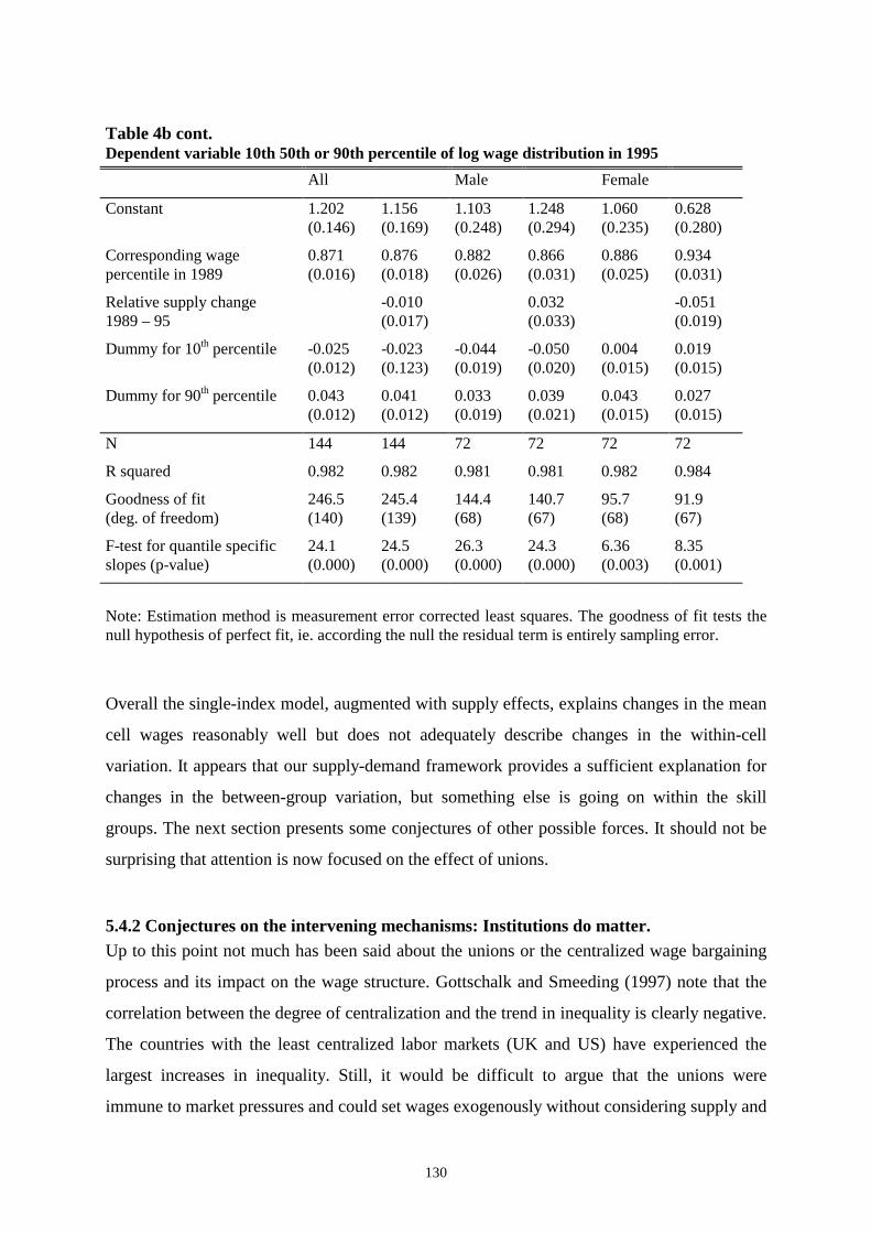
130

Table 4b cont.Dependent variable 10th 50th or 90th percentile of log wage distribution in 1995

All Male Female

Constant 1.202(0.146)

1.156(0.169)

1.103(0.248)

1.248(0.294)

1.060(0.235)

0.628(0.280)

Corresponding wagepercentile in 1989

0.871(0.016)

0.876(0.018)

0.882(0.026)

0.866(0.031)

0.886(0.025)

0.934(0.031)

Relative supply change1989 – 95

-0.010(0.017)

0.032(0.033)

-0.051(0.019)

Dummy for 10th percentile -0.025(0.012)

-0.023(0.123)

-0.044(0.019)

-0.050(0.020)

0.004(0.015)

0.019(0.015)

Dummy for 90th percentile 0.043(0.012)

0.041(0.012)

0.033(0.019)

0.039(0.021)

0.043(0.015)

0.027(0.015)

N 144 144 72 72 72 72

R squared 0.982 0.982 0.981 0.981 0.982 0.984

Goodness of fit(deg. of freedom)

246.5(140)

245.4(139)

144.4(68)

140.7(67)

95.7(68)

91.9(67)

F-test for quantile specificslopes (p-value)

24.1(0.000)

24.5(0.000)

26.3(0.000)

24.3(0.000)

6.36(0.003)

8.35(0.001)

Note: Estimation method is measurement error corrected least squares. The goodness of fit tests thenull hypothesis of perfect fit, ie. according the null the residual term is entirely sampling error.

Overall the single-index model, augmented with supply effects, explains changes in the mean

cell wages reasonably well but does not adequately describe changes in the within-cell

variation. It appears that our supply-demand framework provides a sufficient explanation for

changes in the between-group variation, but something else is going on within the skill

groups. The next section presents some conjectures of other possible forces. It should not be

surprising that attention is now focused on the effect of unions.

5.4.2 Conjectures on the intervening mechanisms: Institutions do matter.Up to this point not much has been said about the unions or the centralized wage bargaining

process and its impact on the wage structure. Gottschalk and Smeeding (1997) note that the

correlation between the degree of centralization and the trend in inequality is clearly negative.

The countries with the least centralized labor markets (UK and US) have experienced the

largest increases in inequality. Still, it would be difficult to argue that the unions were

immune to market pressures and could set wages exogenously without considering supply and

131

demand conditions. Therefore, treating the wage bargaining mechanism as an exogenous

factor could be quite misleading.

Institutions do have a crucial role in wage setting. The wage bargaining system is highly

centralized in Finland. Since 1969 wage negotiations have been co-ordinated on the national

level and annual wage contracts covered all unions. Union wage agreements are also binding

for the non-union workers. In order to provide an explanation for the change in inequality,

there should have been a change in the wage setting system. However, during the period

under the study, no major changes occurred. Membership in the labor unions actually grew

during the 1980's, especially among the white-collar workers (Kyntäjä, 1993). Yet, there has

been some variation in the degree of centralization from year to year. Between 1977 and 1995

there were five occasions when no central agreement was achieved and wages were

negotiated at the industry level. Also, even in years when a national central agreement was

negotiated not all unions accepted the contract.

Ruutu (1997) has calculated the share of the union members that were outside the central

bargain in each round of the wage negotiations. This share shows a strong correlation with the

increase in wage dispersion. Figure 6 shows the change in the 90/10 wage differential in three

year intervals13 with the average fraction of union members outside the central bargains that

were in force during the same periods. With just six observations, the statistical significance

is questionable but the visual impression is striking. Of course, this association does not

imply a causal relationship. The changes in inequality observed in Figure 6 could also fairly

well match other time series, such as the growth rate of the GNP. In fact, Ruutu (1997) shows

that the unions are more likely to opt out from the central bargain if the unemployment has

been low, or the economic growth has been high in the year before the wage negotiations.

13Inequality measures were not available for the years -78, -79, -81, -82, -84 and -85. Focusing onthree year intervals skips these years.

132

Figure 6. Changes in aggregate wage dispersion and centralization of wage bargaining.Note: Centralization index (vertical bars) is a three year average of the percentage of all unionmember who were outside central agreement. It includes members of SAK unions which did notaccept the centrally negotiated bargain and members of other central union organizations (STTK,AKAVA) in the years when more than one central bargain was negotiated. Source: Ruutu (1997).Inequality indices (thin lines) were calculated from OECD data shown in Figure 2 and refer to thethree year change in the decile ratios.

Bearing in mind qualifications about the direction of causality, the results still suggest that the

changes in the bargaining system may provide the missing piece for understanding the

changes in the wage distribution. The growing within-group wage dispersion in the end of the

1980's might well be related to the decentralization, as well as the supply and demand factors.

The contraction of the wage distribution in the early 1990's occurred during four successive

rounds of nationwide wage negotiations. After industry level bargains in 1994 and 1995 wage

differences increased again.

133

5.5 Concluding comments

In this paper, a simple supply and demand framework is developed in order to explain the

observed changes in the aggregate wage distribution in Finland from 1977 to 1995. A single-

skill model, augmented with supply effects, fits relatively well the data on age/education cell

means, but less well on quantiles. Therefore, it seems that the changes in age and education

related wage differentials can be reasonably explained with just supply and demand factors,

but changes within groups of similar age and education requires more. One possible

explanation is based on changes in the institutional setting.

Comparing different time periods with goodness of fit indices reveals that the augmented

single-skill model performs best in explaining changes in the period from 1983 to 1989.

Changes in the other periods are not as well accounted for. The changes in the wage

distribution during the rapidly increasing unemployment in the 1990's would be particularly

interesting, but its closer examination is outside the scope of this paper. Also, it is clear that

the single-index model cannot account for a relative increase in women's wages. The most

obvious explanation for the increase is the shift in the female skill distribution caused by

increasing labor force participation and increasing amount of work experience.

Most interestingly, very little evidence of increasing demand for skills is found in this study.

At least changes in the demand for skills do not show as widening skill related wage

differences. Consequences of such apparently rigid wage structure for relative employment of

different skill groups, particularly during high unemployment, will be an interesting topic for

further research.

134

References

Asplund, R. (1994) ''Palkkaerot Suomen Teollisuudessa,” The Research Institute of the Finnish

Economy, Series B 91.

Asplund, R (1997) ''The Disappearing Wage Premium of Computer Skills,'' The Research Institute of

the Finnish Economy, Discussion Papers 619.

Atkinson, A., Smeeding, T. and Rainwater, L. (1995) “Income Distribution in OECD Countries:

Evidence from the Luxembourg Income Study,” OECD Social Policy Studies 18.

Bell, B. (1996) “Skill-biased Technical Change and Wages: Evidence from a Longitudinal Data Set,”

Working Paper 25, Nuffield College, Oxford.

Blackburn, M. and Neumark, D. (1993) “Omitted-ability Bias and the Increase in the Return to

Schooling,” Journal of Labor Economics 11, 521-544.

Bound, J. and Johnson, G. (1992) ''Changes in the Structure of Wages in the 1980's: An Evaluation of

Alternative Explanations,'' American Economic Review 82, 371-392.

Card, D. and Lemieux, T. (1996) ''Wage Dispersion, Returns to Skill, and Black-White Wage

Differentials,'' Journal of Econometrics 74, 319-361.

Deaton, A. (1985) ''Panel Data from Time Series of Cross Sections,'' Journal of Econometrics 30,

109-126.

DiNardo, J., Fortin, N. and Lemieux, T. (1996) ''Labor Market Institutions and the Distribution of

Wages 1973-1992: A Semiparametric Approach,'' Econometrica, 64, 1001-1044.

Edin, P-A. and Holmlund B. (1995) ''The Swedish Wage Structure: The Rise and Fall of Solidarity

Wage Policy?'' in Freeman, R. and Katz, L. eds. Differences and Changes in Wage Structures.

Chicago: University of Chicago Press.

Eriksson T. and Jäntti M. (1997) ''The Distribution of Earnings in Finland 1971-1990,'' European

Economic Review 41, 1763-1779.

Fuller, W. (1987) ''Measurement Error Models,'' New York: Wiley.

Gottschalk, P. and Smeeding, T. (1997) ''Cross-National Comparisons of Earnings an Income

Inequality,'' Journal of Economic Literature 35, 633-687.

Hamermesh, D. (1993) ''Labor Demand,'' Princeton: Princeton University Press.

Juhn, C., Murphy, K. and Pierce, B. (1993) ''Wage Inequality and the Rise in Returns to Skill,''

Journal of Political Economy 101, 410- 442.

135

Katz, L. and Murphy, K. (1992) ''Changes in Relative Wages, 1963-1987: Supply and Demand

Factors,'' Quarterly Journal of Economics 107, 35-78.

Krueger, A. (1993) ''How Computers Have Changed the Wage Structure? Evidence from Microdata,

1984-1989,'' Quarterly Jornal of Economics 108.

Kyntäjä, T. (1993) ''Tulopolitiikka Suomessa: Tulopoliittinen Diskurssi ja Instituutiot 1960-luvulta

1990-luvun Kynnykselle,'' Helsinki: Gaudeamus.

Levy, F. and Murnane, R. (1992) ''U.S. Earnings Levels and Earnings Inequality: A Review of Recent

Trends and Proposed Explanations,'' Journal of Economic Literature 30, 1333-1381.

OECD (1996) ''Earnings Inequality, Low-Paid Employment and Earnings Mobility,'' chapt. 3, in

Employment Outlook. Paris: Organization for Economic Co-operation and Development.

OECD (1995) ''Education at Glance'' Paris: Organization for Economic Co-operation and

Development.

SVT (1997). ''Official Statistics of Finland,'' Statistics Finland, Education 1997:1, Helsinki.

Ruutu, J. (1997) ''The Finnish System of Collective Agreements, Wages and Inflation,'' The Research

Institute of the Finnish Economy, Discussion Papers 611.

Uusitalo, R. (1996) ''Return to Education in Finland,'' Department of Economics, University of

Helsinki, Research Reports 71.

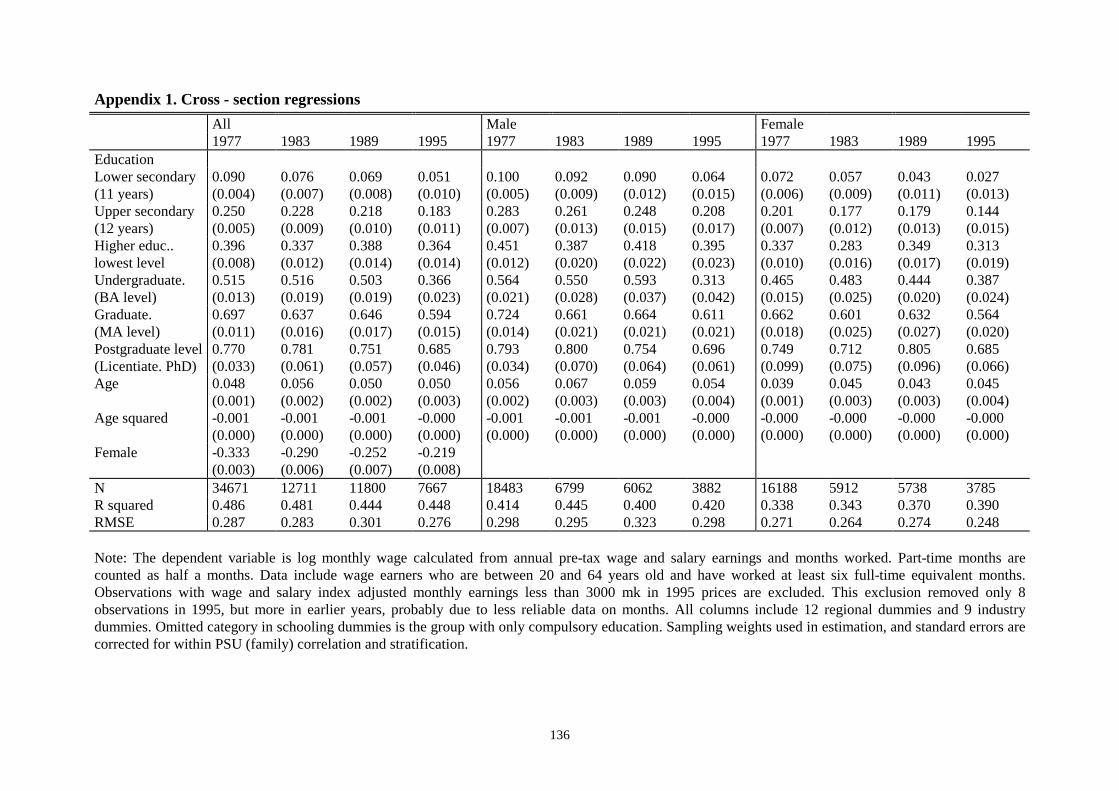
136

Appendix 1. Cross - section regressionsAll Male Female1977 1983 1989 1995 1977 1983 1989 1995 1977 1983 1989 1995

EducationLower secondary(11 years)

0.090(0.004)

0.076(0.007)

0.069(0.008)

0.051(0.010)

0.100(0.005)

0.092(0.009)

0.090(0.012)

0.064(0.015)

0.072(0.006)

0.057(0.009)

0.043(0.011)

0.027(0.013)

Upper secondary(12 years)

0.250(0.005)

0.228(0.009)

0.218(0.010)

0.183(0.011)

0.283(0.007)

0.261(0.013)

0.248(0.015)

0.208(0.017)

0.201(0.007)

0.177(0.012)

0.179(0.013)

0.144(0.015)

Higher educ..lowest level

0.396(0.008)

0.337(0.012)

0.388(0.014)

0.364(0.014)

0.451(0.012)

0.387(0.020)

0.418(0.022)

0.395(0.023)

0.337(0.010)

0.283(0.016)

0.349(0.017)

0.313(0.019)

Undergraduate.(BA level)

0.515(0.013)

0.516(0.019)

0.503(0.019)

0.366(0.023)

0.564(0.021)

0.550(0.028)

0.593(0.037)

0.313(0.042)

0.465(0.015)

0.483(0.025)

0.444(0.020)

0.387(0.024)

Graduate.(MA level)

0.697(0.011)

0.637(0.016)

0.646(0.017)

0.594(0.015)

0.724(0.014)

0.661(0.021)

0.664(0.021)

0.611(0.021)

0.662(0.018)

0.601(0.025)

0.632(0.027)

0.564(0.020)

Postgraduate level(Licentiate. PhD)

0.770(0.033)

0.781(0.061)

0.751(0.057)

0.685(0.046)

0.793(0.034)

0.800(0.070)

0.754(0.064)

0.696(0.061)

0.749(0.099)

0.712(0.075)

0.805(0.096)

0.685(0.066)

Age 0.048(0.001)

0.056(0.002)

0.050(0.002)

0.050(0.003)

0.056(0.002)

0.067(0.003)

0.059(0.003)

0.054(0.004)

0.039(0.001)

0.045(0.003)

0.043(0.003)

0.045(0.004)

Age squared -0.001(0.000)

-0.001(0.000)

-0.001(0.000)

-0.000(0.000)

-0.001(0.000)

-0.001(0.000)

-0.001(0.000)

-0.000(0.000)

-0.000(0.000)

-0.000(0.000)

-0.000(0.000)

-0.000(0.000)

Female -0.333(0.003)

-0.290(0.006)

-0.252(0.007)

-0.219(0.008)

N 34671 12711 11800 7667 18483 6799 6062 3882 16188 5912 5738 3785R squared 0.486 0.481 0.444 0.448 0.414 0.445 0.400 0.420 0.338 0.343 0.370 0.390RMSE 0.287 0.283 0.301 0.276 0.298 0.295 0.323 0.298 0.271 0.264 0.274 0.248

Note: The dependent variable is log monthly wage calculated from annual pre-tax wage and salary earnings and months worked. Part-time months arecounted as half a months. Data include wage earners who are between 20 and 64 years old and have worked at least six full-time equivalent months.Observations with wage and salary index adjusted monthly earnings less than 3000 mk in 1995 prices are excluded. This exclusion removed only 8observations in 1995, but more in earlier years, probably due to less reliable data on months. All columns include 12 regional dummies and 9 industrydummies. Omitted category in schooling dummies is the group with only compulsory education. Sampling weights used in estimation, and standard errors arecorrected for within PSU (family) correlation and stratification.