rong liu monitoring, modeling, and control of …
TRANSCRIPT

RONG LIUMONITORING, MODELING, AND CONTROL OF NUTRIENT REMOVAL IN THE
ACTIVATED SLUDGE PROCESS(Under the Direction of M. BRUCE BECK)
The activated sludge process has been one of the most widely used biological
processes for treating wastewater containing inorganic and organic pollutants. However,
increased process complexity in the activated sludge system makes it more vulnerable to
external disturbances, such as large variations in flow. Under these circumstances,
analysis in mathematical form stands out with the potential benefits of improving
understanding of process performance under dynamic conditions, and optimizing
operation to treat greater volumes of wastewater, to deal with higher variability in
influent load, and meet even more stringent discharge standards.
The objectives of this research are accordingly (i) to develop an understanding of
the dynamic behavior of the biological nutrient removal processes in the activated sludge
process and (ii) to determine efficient control strategies to achieve more reliable plant
operation.
The dissertation begins with an extensive review of (i) dynamic behavior of the
process; (ii) dynamic models of the activated sludge processes; and (iii) control schemes
applied to the system. Collection of high-quality data at Athens Wastewater Treatment
Facility No. 2 for an extended period of time is then described. The University of
Georgia’s Environmental Process Control Laboratory (EPCL) demonstrates enormous
potential in retrieving high-frequency, high-quality field data, which is a prerequisite for
success in the subsequent development of process models and process control strategies
for these systems. A high-order model was then built up to simulate the nutrient removal
processes, including especially a modified means of characterizing transport and mixing
of both solute and particulate matter in the activated sludge system. Subsequently, the
calibrated model was validated to test its robustness of under conditions different from
those of calibration. The model is considered to be acceptable in its performance and thus

adequate for its subsequent application in studies of process control. Using the model
thus identified, a detailed assessment of control strategies for the activated sludge process
has been conducted. This is focused on storm event control. The manipulated control
variables are confined to those routinely used, i.e., recycle rate, wastage rate, step-feed,
and step-sludge. Even so, the operational flexibility of the activated sludge process can
thus be fully exploited.
INDEX WORDS: Activated sludge system, Real time monitoring, Dynamic modeling,
Signal processing, Model calibration, Model validation, Control
strategies

MONITORING, MODELLING, AND CONTROL OF NUTRIENT REMOVAL IN THE
ACTIVATED SLUDGE PROCESS
by
RONG LIU
B.E., East China University of Science and Technology, China, 1993
M.E., East China University of Science and Technology, China, 1996
A Dissertation Submitted to the Graduate Faculty of The University of Georgia in Partial
Fulfillment of the Requirements for the Degree
DOCTOR OF PHILOSOPHY
ATHENS, GEORGIA
2000

© 2000
Rong Liu
ALL Rights Reserved

MONITORING, MODELLING, AND CONTROL OF NUTRIENT REMOVAL IN THE
ACTIVATED SLUDGE PROCESS
by
RONG LIU
Approved:
Major Professor: Dr. M. B. Beck
Committee: Dr. Todd Rasmussen Dr. Rhett Jackson
Dr. Matt Smith Dr. William Kisaalita
Electronic Version Approved:
Gordhan L. PatelDean of the Graduate SchoolThe University of GeorgiaDecember 2000

iv
ACKNOWLEDGEMENTS
First of all, I want to acknowledge my major professor, Dr. M. B. Beck, for his
kindness, generosity, consistent involvement, and encouragement throughout my Ph.D
career. He certainly deserves an awful lot more than simply a few words of appreciation.
I want to thank all my friends for their professional and personal support through
these years as well. Just to mention a few here, the successful sampling campaign with
the EPCL at the Athens Wastewater Treatment Facility No.2 would not have been a
success without Stefan Winkler’s hard work, from commissioning of the EPCL untill his
departure at the end of 1997, and Robert Lawler’s assistance during the period of the
sampling campaign. Thanks are also due to the staff at the Athens Wastewater Treatment
Facility No.2 for their cooperation during the data-collection, and permission to use their
field data, without which this dissertation could not have been completed. I also want to
thank Dr. Beck’s administrative coordinator, Ms. Jenny Yearwood, for her true friendship
in seeing me through all the hardships. Appreciation is also extended to Wei Zeng and his
wife, Tongrui, for their kindness and help.
All my family is to be acknowledged for their constant support, especially my
parents and parents-in-law.
Finally, my deepest appreciation goes to my husband, Yu. Without his support, I
would not have come such a long way. He not only has to be thanked, but also deserves
part of the credit.

v
TABLE OF CONTENTS
Page
ACKNOWLEDGEMENTS................................................................................................ iv
CHAPTER
1. INTRODUCTION ..............................................................................................1
1.1 BACKGROUND ................................................................................1
1.2 OBJECTIVES OF RESEARCH.........................................................4
1.3 CONTENTS AND CONTRIBUTIONS.............................................4
2. DYNAMICS, MODELING, AND CONTROL OF THE ACTIVATED
SLUDGE PROCESS—A REVIEW ...................................................................7
2.1 INTRODUCTION ..............................................................................7
2.2 DYNAMIC BEHAVIOR....................................................................7
2.3 MODELS ..........................................................................................21
2.4 CALIBRATION ...............................................................................35
2.5 SENSITIVITY ANALYSIS .............................................................37
2.6 PROCESS CONTROL .....................................................................38
2.7 CONCLUSIONS ..............................................................................44
3. DATA COLLECTION AND DATA PRE-PROCESSING .............................45
3.1 INTRODUCTION ............................................................................45
3.2 SAMPLING CAMPAIGN................................................................45
3.3 ENVIRONMENTAL PROCESS CONTROL LABORATORY
(EPCL)..............................................................................................52
3.4 INTRODUCTION TO SMOOTHING ALGORITHM OF TVP
ANALYSIS TOOLBOX...................................................................64
3.5 EXAMPLE OF SMOOTHED MODEL INPUT DATA..................65
vi
3.6 CONCLUSIONS ..............................................................................72
4. MODEL DEVELOPMENT..............................................................................73
4.1 INTRODUCTION ............................................................................73
4.2 PURPOSE OF THE MODEL...........................................................73
4.3 OVERALL ARRANGEMENT OF THE MODEL..........................74
4.4 AERATOR MODEL STRUCTURE................................................80
4.5 SECONDARY CLARIFIER MODEL STRUCTURE...................100
4.6 DISCUSSIONS...............................................................................106
4.7 CONCLUSIONS ............................................................................106
5. MODEL CALIBRATION, VALIDATION, AND SENSITIVITY
ANALYSIS......................................................................................................108
5.1 INTRODUCTION ..........................................................................108
5.2 MODEL CALIBRATION RESULTS AND DISCUSSIONS .......108
5.3 MODEL VALIDATION ................................................................131
5.4 PARAMETER ESTIMATION.......................................................143
5.5 SENSITIVITY ANALYSIS ...........................................................146
5.6 CONCLUSIONS ............................................................................151
6. DEVELOPMENT AND EVALUATION OF PROCESS CONTROL
STRATEGIES.................................................................................................152
6.1 INTRODUCTION ..........................................................................152
6.2 SPECIFICATION OF THE ASSESSMENT..................................152
6.3 DETAILED SPECIFICATION OF THE CONTROL
ALGORITHMS ..............................................................................161
6.4 SIMULATION RESULTS AND EVALUATION OF CONTROL
STRATEGIES.................................................................................172
6.5 FURTHER CONSIDERATIONS ..................................................194
6.6 CONCLUSIONS ............................................................................197

vii
7. CONCLUSIONS AND RECOMMENDATIONS..........................................199
7.1 INTRODUCTION ..........................................................................199
7.2 CONCLUSIONS ............................................................................199
7.3 RECOMMENDATIONS FOR FUTURE WORK .........................200
REFERENCES ...............................................................................................................202
APPENDICES .................................................................................................................242
I. QA/QC PROCEDURES FOR THE MONITORS .........................................242
II. DAILY MAINTENANCE CHECKLIST OF THE INSTRUMENTS
IN EPCL.........................................................................................................251

1
CHAPTER 1
INTRODUCTION
1.1 BACKGROUND
Over the past decades eutrophication of surface water as a result of nutrient
discharges has become manifest. Occurrences of elevated levels of nitrogen and
phosphorus in various chemical forms give rise to algae blooms, which cause oxygen
depletion, odor problems, aesthetic problems and serious disturbance of aquatic
ecosystems. Consequently, legislation has imposed stricter demands on effluent nutrients.
The nutrients present in the wastewater can be removed either physically or converted by
means of chemical or biological processes. Due to its consistent efficiency in removing
inorganic and organic pollutants from wastewater, activated sludge is currently one of the
most widely used biological processes for treating domestic wastewater. However,
increased process complexity in the activated sludge system makes it more vulnerable to
disturbances such as large variations in flow, load and temperature. Sometimes the
process loses its stability suddenly for no obvious reason, which underlines the
importance of taking operational elements into consideration during the design process
(Andrews, 1974). Thus there is a continuous need to better understand this biological
wastewater treatment process. One strategy to fulfill this need is to model this process in
mathematical form, which offers a number of potential benefits:
q Improve understanding of process performance under dynamic conditions;
q Optimize design of wastewater treatment plants;
q Optimize operation (prevent process failure and enhance treatment efficiency) to treat
larger volumes of water, to deal with higher variability in influent load, and meet
even more stringent discharge standards (Lijklema, 1973).
2
Reliable design and operation of biological wastewater treatment systems
demands effective modeling of the various nutrient removal processes involved. Steady-
state models are normally used for process design, and they can also be used for
prediction of process performance. Due to the dynamic nature of biological processes and
the unsteady disturbances to which they are subject, dynamic models are essential for
describing the operation of biological wastewater treatment processes (for example,
activated sludge process), and establishing the most effective real-time control strategy.
Therefore, mathematical analysis is widely used to optimize or pinpoint the most cost-
effective operational solution. By imposing feasible control strategies on the activated
sludge system, wastewater treatment plants can save money from more reliable and cost-
effective operation, and can, in principle, save even more money from deferring plant
capacity expansion. Carucci et al. (1999) optimized the operating of a large wastewater
treatment plant by shutting down one of the three treatment lines and overloading the
other two. The potential cost savings of the vacuum-exhaust control (VEC) strategy for
the city of Houston, Texas, 69th Street Treatment Complex was examined by Clifft et al.
(1988). At 80% of design loading VEC was found to provide an oxygen-utilization
efficiency of 94.9% as compared to 77.0% for the conventional control method. Based on
the expected turn-down capability of Houston’s oxygen production facilities, their
simulations indicated that the VEC strategy would more than double the possible cost
savings of the conventional control method. Additional savings at 80% and 100% of
design loading were estimated to be $113,000 and $46,500 per year for the VEC strategy.
As a rule of thumb, constructing a good mathematical model requires high-quality real
world data of sufficient quantity. Reliable, on-line, ‘intelligent’ instruments can certainly
satisfy this demand. However, lack of either first-class high-frequency real-time field
data, reflecting the process responses to dynamic perturbations, or reasonably good
process models, has long prevented environmental scientists from achieving better
reconciliation of mathematical models with real data (Beck, 1986).

3
The University of Georgia’s recently commissioned Environmental Process
Control Laboratory (EPCL) opens up an opportunity to correct the above-mentioned data
limitation. It has proven to be an effective tool in revealing actual process performance
on-line. As an integrated facility equipped with multiple automatic instruments, it can be
deployed in the wastewater treatment plant or other features of the aquatic environment,
such as an aquaculture pond, for continuous sampling campaigns over extended periods,
typically of the order of months. The data thus retrieved provide a solid foundation for
subsequent model development, calibration, and application (Beck and Liu, 1998).
In 1986, the International Association of Water Quality (IAWQ), now
International Water Association (IWA), published the Activated Sludge Model No. 1
(ASM1) (Henze et al., 1986), which describes biological nitrification and denitrification
processes in the activated sludge system. In 1999, its most recent successor, the ASM3
(Gujer et. al., 1999) was published. ASM3 relates to the ASM1 and corrects for some
defects of ASM1. As an extension to ASM1, the IWA published the ASM2 (Gujer et. al.,
1995) in 1995. ASM2’s successor, the ASM2d (Henze et. al., 1999), was later published
in 1999. In addition to what is already described in ASM1/ASM3, enhanced biological
phosphorus removal (EBPR) and two other chemical processes are incorporated in
ASM2/ASM2d. The completeness of ASM2/ASM2d is certainly a significant
contribution. They represent the state of art in modeling the activated sludge process.
However, they have not been successfully calibrated against extended experimental
observations collected from actual wastewater treatment processes. They are definitely
not universally best for every single practical application, and will certainly suffer from
problems of a lack of identifiability in model calibration. In other words, it is not possible
to find a uniquely best set of parameter values for the model. Rather than a final answer,
ASM2/ASM2d establishes a platform for further model development under different
circumstances (Gujer et. al., 1995).

4
1.2 OBJECTIVES OF RESEARCH
The primary objectives of this research are to:
q Develop an understanding of the dynamic behavior of the biological nutrient removal
processes in the activated sludge system with data acquired with the EPCL;
q Determine efficient control strategies to achieve more reliable plant operation.
These goals are achieved via the following steps:
q Retrieval of first-class high-frequency real-time field data over an extended period of
time through a case-study experiment at the Athens Wastewater Treatment Facility #2
in Athens, GA;
q Signal pre-processing directed at the goal of model development;
q Development of a new dynamic model to simulate various nutrient removal processes
in the activated sludge system. The detailed steps include:
• Characterization of solute and particulate transport (through the aeration tank and
secondary clarifier);
• Development of nitrogen removal model (nitrification and denitrification);
• Development of model for carbonaceous compound removal;
• Development of phosphorus removal model.
q Development and assessment of feasible control strategies for operational
management of the activated sludge process based on the resulting model.
1.3 CONTENTS AND CONTRIBUTIONS
There are seven chapters in the dissertation. This chapter has set out the
background and objectives of the research.
In Chapter 2, the nature of the dynamic behavior of the activated sludge process is
reviewed and presented. Subsequently, aspects of dynamic models and process control
strategies for the activated sludge system are collected from the literature.

5
Following this review, three aspects are dealt with in Chapter 3. One aspect is the
sampling campaign arrangements at the Athens Wastewater Treatment Facility #2,
including case study site description, sampling regime and retrieved data streams. The
second aspect is the Environmental Process Control Laboratory (EPCL), including its
hardware, software, and quality assurance and quality control (QA/QC) aspects. The
sampling campaign succeeded in acquiring first-class extensive experimental results
collected from an actual wastewater treatment process. Such comprehensive data, to the
best of our knowledge, exist nowhere else in the published literature. The third aspect
deals with data pre-processing, which concerns how raw data are processed without bias
before being presented for model development. This work also provides an opportunity
for assessing transport and mixing properties of both solute and particulate materials as
they pass through the bioreactor and secondary clarifier of the activated sludge process,
although these features will not be covered in this dissertation.
Chapter 4 deals with the subject of model development, with emphasis laid on
characterization of solute and particulate transport through the aeration tank and
secondary clarifier, together with nitrification and denitrification model development.
This is where the proposed model is significantly different from what has usually been
reported in the literature. This new model substantially enhances our capability to match
the field data.
Following Chapter 4, Chapter 5 deals with model calibration. Complete
calibration was carried out for the nitrification and denitrification processes. The overall
strategy was to achieve successful nitrification fitting, because it is the best defined
process and is most sensitive to external upsets of the various biological processes.
Within the restricted span of the dissertation, efforts were then made to obtain acceptable
carbon and phosphorus calibrations.
Based on the model thus identified, process control strategies are simulated in
Chapter 6 to assess their effectiveness in improving plant operations during storm events.

6
Advanced algorithms are tested to assess whether the process can be effectively
controlled using the routinely manipulated control variables.
The principle conclusions of this research and recommendations for future work
are given in Chapter 7.

7
CHAPTER 2
DYNAMICS, MODELING, AND CONTROL OF THE
ACTIVATED SLUDGE PROCESS—A REVIEW
2.1 INTRODUCTION
The purpose of this chapter is to provide a general view of what has been captured
in the literature on dynamics, modeling, and control of the activated sludge process.
The chapter is organized as follows. In section 2.2, the dynamic behavior of the
activated sludge process is summarized. Based on a comprehensive understanding of
process behavior thus provided, dynamic modeling of the activated sludge process is
reviewed in section 2.3, which includes the reactor model (section 2.3.1) and secondary
clarifier model (section 2.3.2). Section 2.4 deals with model calibration. Sensitivity
analysis and control of the activated sludge process are then reviewed in sections 2.5 and
2.6 respectively.
2.2 DYNAMIC BEHAVIOR
2.2.1 Activated Sludge Process
The activated sludge process is a suspended growth system consisting of two
stages, aeration and sludge/liquid separation. In theory, in the aeration stage extremely
high rates of microbial growth and respiration can be achieved with unlimited food and
oxygen, resulting in the utilization of available inorganic and organic matter to produce
oxidized end products or the biosynthesis of new microorganisms. Air is added to the
system either by surface agitators or via diffusers. Aeration has dual functions: supply of
oxygen to the aerobic microorganisms for respiration, and maintenance of the microbial
flocs in a continuous state of agitated suspension, ensuring maximum contact between the
8
surfaces of the flocs and the substrates in wastewater. The mixed liquor (mixture of
wastewater and microbial biomass) is subsequently displaced into secondary clarifiers.
This is the final stage in the activated sludge process, where the flocculated biomass
settles rapidly out of suspension to the bottom of the secondary clarifiers forming sludge
under quiescent conditions, with the clarified effluent, which should be free of solids,
discharged as the final effluent. It is a characteristic of the activated sludge process that a
fraction of the settled sludge is recycled back to the aeration tank to achieve efficient
nutrient removal. The surplus solids are wasted.
2.2.2 Microbial Biomass
Mixed liquor suspended solids (MLSS) concentration is a crude measurement of
the amount of biomass within the aeration tank. In biological wastewater treatment a
wide variety of microorganisms are found, including viruses, bacteria, fungi and
protozoa. But the most widely occurring and abundant group of microorganisms is
bacteria, and it is this group of biomass that is most important in terms of utilizing the
inorganic and organic substrate in the wastewater.
The inorganic and organic matter in wastewater is utilized in a series of enzymatic
reactions. Enzymes are pure proteins or proteins combined with either an inorganic or
low molecular weight organic molecule. Enzymes act as catalysts to form complexes
with the organic substrate, which they subsequently convert to a specific product. The
enzyme is then released to catalyze the same reaction over and over again. Enzymes have
such a high degree of substrate specificity that bacterial cells must produce a different
enzyme for each substrate utilized. There are basically two types of enzymes. Extra-
cellular enzymes convert substrates extracellularly into forms that can be taken into the
cell for further breakdown by the intracellular enzymes, which are involved in synthesis
and energy reactions within the cell. Normally the product of one enzymatic reaction

9
immediately combines with another enzyme until the final end product required by the
cell is reached after a sequence of enzyme-substrate interactions (Gray, 1990).
The most commonly used model, relating microbial growth to substrate
utilization, is the Monod relationship. It is assumed in this model that the growth rate of
biomass is not only a function of microorganism concentration, but also of limiting
substrate concentrations. The relationship between the specific growth rate of biomass
(µ) and the residual concentration of growth-limiting substrate (S) is described as
follows:
where,
µm−Maximum specific growth rate (d-1) of microorganisms at saturation concentration of
growth limiting substrate;
S−Growth limiting substrate concentration (mg/L);
Ks−Saturation coefficient (mg/L) which is the concentration of growth-limiting substrate
at which the specific growth rate of microorganisms equals one-half of the maximum
specific growth rate (µ = µm / 2).
2.2.3 Inorganic and Organic Substrate
Organic Substrate
Wastewater normally contains different kinds of organic matter, which all have in
common at least one carbon atom (and thus are also known as carbonaceous compounds).
They can be oxidized either chemically or biologically to yield carbon dioxide and water.
Through these reactions the microorganisms obtain the energy necessary for their growth.
A measurement of each individual organic matter is impossible. Therefore different
collective analyses, such as Total Organic Carbon (TOC), Chemical Oxygen Demand
(COD), and Biochemical Oxygen Demand (BOD), are adopted.
SKS
sm +
= *µµ

10
Inorganic Substrate (Nitrogen and Phosphorus)
Nitrogen and phosphorus together are known as nutrients in the wastewater.
Nitrogen in sewage arises primarily from metabolic conversions of excreta-derived
compounds, whereas 50% or more of the phosphorus arises from synthetic detergents
(Gray, 1990). The principal forms of nutrients occurring in municipal wastewater are:
NH4+ (ammonium), NO2
- (nitrite), NO3- (nitrate), and PO4
3- (orthophosphate). Perhaps the
most widespread example of pollution through nitrogen and phosphorus discharges
occurs through its ability to promote growth of algae. Significant seasonal and annual
trends in effluent NH4+ variability were found in six out of seven nitrification plant
studies in Ohio (Rossman, 1984).
2.2.4 Biochemical and Chemical Reactions
2.2.4.1 Nitrification
The microbial oxidation of ammonium occurs in two distinct stages, each of
which involves different species of nitrifying bacteria. The first stage is the oxidation of
ammonium to nitrite by Nitrosomonas. In the second stage nitrite is oxidized to nitrate by
Nitrobacter. In practice it is the oxidation of ammonium that is generally believed to be
the rate-limiting step in the overall process. The whole nitrification process requires a
high input of oxygen.
In the context of sequential Nitrosomonas-Nitrobacter activity and a low-level of
nitrite presence, the conversion of ammonium to nitrite by Nitrosomonas has long been
deemed as the rate-limiting step for complete conversion of ammonium to nitrate
(Benefield and Randall, 1980). Several studies, however, have observed the presence of a
considerable amount of nitrite, a so-called ‘nitrite buildup’ (Silverstein and Schroeder
1983; Randall and Buth 1984; Abeling and Seyfried 1992; Mauret 1996). The possible
conditions under which an elevated nitrite concentration might be realized in a
nitrification system are reduced temperatures, limiting oxygen presence, elevated pH,

11
free ammonia presence, elevated solids wastage, acute process loading, and unusual
nitrate reduction (Alleman, 1984; Balmelle et al., 1992; Mauret et al., 1996; Surmacz-
Górska et al., 1997). In a similar study, Yang and Alleman (1992) discovered that nitrite
buildup did not correlate well with either dissolved oxygen concentration or free
ammonia. The concentration of free hydroxylamine and other intermediates in
nitrification were the principal factor behind nitrite accumulation in batch nitrifying
systems. Some researchers took inhibition of nitrite oxidation to nitrate as a more
economical method of nitrogen removal in comparison with the traditional method of
nitrogen removal (Turk and Mavinic 1989; Akunna et al., 1993).
Oxidation of nitrite by Nitrobacter in a chemostat system was reported to depend
strongly on the presence of the ammonium oxidizer Nitrosomonas (Gee et al., 1990).
Nitrite oxidation in the absence of ammonium required a 10-day retention time, whereas
complete oxidation of ammonium was achieved at a retention time of 2.7 days. Reduction
of nitrite and nitrate was reported to occur simultaneously and was dependent on the
oxidation of ferrous to ferric iron (Nielsen and Nielsen, 1998).
Organic matter is known to “poison’ the nitrifiers, so that increases in organic
loading results in rapid decreases in the rate of nitrification. This is probably due to the
increased activity of heterotrophs, which, because of their more rapid growth rates,
successfully out-compete the nitrifying bacteria for access to dissolved oxygen and
nutrients. This direct competition from heterotrophs is a major cause of nitrification
failure (Gray, 1990; Henze et al., 1995b).
2.2.4.2 Denitrification
This is a biological process which occurs under low dissolved oxygen (anoxic)
conditions and when a suitable carbon source is available. Oxidized forms of nitrogen,
nitrite or nitrate, are reduced to molecular nitrogen form. The rate of denitrification
occurring in secondary clarifiers, characterized by flocs buoyed up to the surface by

12
nitrogen gas, is extremely low due to a number of factors, the most important being
insufficient carbon substrate for metabolism (Gray, 1990).
Two studies emphasized the role of denitrification in oxidation ditches (Huang
and Drew, 1985; Rittmann and Langeland, 1985). In both investigations, significant
denitrification was observed in the anoxic zone. Mateju et al. (1992) reviewed biological
denitrification including its microbiology, reaction stoichiometry, bioreactors, and unit
processes. Theoretically, denitrification can only proceed under anoxic conditions where
a suitable carbon source, such as methanol, is available. Nitrate is progressively reduced
to nitrogen gas by heterotrophic bacteria via the following route:
NO3 NO2 NO N2O N2
Nitrate Nitrite Nitric Oxide Nitrous Oxide Nitrogen
The enzymes associated with denitrification are synthesized when conditions
become advantageous for denitrification (Knowles, 1982). However, it has been shown
that denitrification can also occur with certain species in the presence of oxygen
(Meiberg et al., 1980). Casey et al. (1994) found that aerobic denitrification only
proceeded with nitrite, but not with nitrate and was enhanced under conditions of low
readily biodegradable substrate in the aerobic phase. The influence of oxygen
concentration (Krul and Veeningen, 1977; Simpkin and Boyle, 1988; Downes, 1988;
Kokufuta et al., 1988), pH (Allison and MacFarlane, 1989), temperature (Lewandowski,
1982), nitrate, and intermediate product concentrations (Skrinde and Bhagat, 1982;
Snyder et al., 1987) on denitrification performance have been investigated in detail.
Denitrification rates by activated sludge increased from 0.001 to 0.02 mg N/mg MLSS/h
in a solution containing 250 mg/L NO2 when the pH was increased from 6 to 8 (Glass et
al., 1997). Thomsen et al. (1994) demonstrated that pH significantly affected intermediate
accumulation in denitrification. At pH 5.5 nitrate, significant quantities of nitrite, and

13
N2O were formed, whereas at pH 8.5 lower concentrations of intermediate products were
formed. Batch tests determined that denitrification could occur at a DO concentration of
up to 0.11 mg/L (Eliosov et al. 1997). Two models of denitrification intermediates were
presented by Wild et al. (1995). Model I included the reduction of nitrate, nitrite, and
nitrous oxide with noncompetitive inhibition by O2 and NO2-. To improve the fitting of
data, Model II incorporated the process of synthesis and decay of denitrification enzymes
and the component “enzyme saturation coefficient.” It was shown that increasing the
anoxic zone DO concentration from 0 to 0.2 mg/L reduced denitrification activity by
approximately 50%. The production and consumption of nitric oxide during
denitrification and its implications were reviewed by Ye et al. (1994).
2.2.4.3 Aerobic Heterotrophic Conversion of Organic Matter
Organic matter in the wastewater can be separated into the following categories:
q Dissolved easily biodegradable organic matter, which can enter the biodegradation
process directly;
q Dissolved biologically inert organic matter, which can not be biodegraded;
q Suspended slowly biodegradable organic matter, which must undergo cell
external hydrolysis before being available for biodegradation;
q Suspended biologically inert organic matter, which cannot be biodegraded.
The most important factors for aerobic conversions of organic compounds are
temperature, oxygen, pH, toxic substances, nitrogen, and phosphorus (Henze et al.,
1995b). Ammonium assimilation by heterotrophs can take place in preference to
nitrification in the aeration tank, with only the surplus ammonium after assimilation
being subject to nitrification. Ammonium assimilation by heterotrophs was demonstrated
to be proportional to COD consumption, and consequently significantly reduced the
availability of ammonium for nitrification. Besides this effect, organic loading produced
an inhibitory effect on ammonium oxidation. Production of toxic compounds by

14
heterotrophs is a possible reason (Hanaki et al., 1990a). Another likely reason for the
inhibitory effect is the localized competition between the heterotrophs and the nitrifiers
for common substrates (Painter, 1977). Research on nitrification at low levels of
dissolved oxygen, with and without organic loading in a suspended-growth reactor,
reveals that a low DO concentration enhances the inhibitory effect of organic loading
through heterotrophic activity on ammonium oxidation.
2.2.4.4 Phosphorus Removal
Phosphorus in the wastewater can be categorized into the following fractions:
q Dissolved inorganic orthophosphate, which is available for immediate biological
metabolism;
q Dissolved inorganic poly-phosphate, which requires further decomposition to the
more assimilable orthophosphate form;
q Dissolved organic phosphate, which requires further decomposition to the more
assimilable orthophosphate form;
q Suspended organic phosphate.
Chemical Phosphorus Removal
In a biological wastewater treatment system precipitation of phosphorus via
addition of metals, such as iron or aluminum salts, is a traditional strategy for phosphorus
removal. But chemicals are very expensive, and the inorganic residues left from the
chemicals can occasionally cause pollution problems. Recent advances in our
understanding have led to the development of biological processes for phosphorus
removal, which is a natural mechanism for removal of phosphorus by the phosphorus-
accumulating bacteria in the mixed liquor. But biological phosphate removal is heavily
dependent on the formation of these polyphosphate-accumulating bacteria. In cases
where the ratio of COD to phosphate in the influent is too low to produce enough
15
biomass for poly-phosphate storage, it is sensible to supplement the biological
phosphorus removal process with chemical phosphorus precipitation.
Biological Phosphorus Removal
The first indication of biological phosphate removal occurring in a wastewater
treatment plant was described by Srinath et al. (1959). They observed that sludge from a
certain treatment plant when aerated exhibited excess phosphorus uptake, more than
needed for cell growth. Milbury et al. (1971) defined some basic requirements for
phosphorus removal by stating that the reactor must operate as a plug-flow scheme, and
the first part of the reactor should not be well aerated. They also found that the sludge had
a maximum capacity for accumulating phosphate. In the second half of the 1970s
research in microbiology expanded. Fuhs and Chen (1975) concluded that bacteria of the
genus Acinetobacter were responsible for biological phosphate removal. They postulated
that an anaerobic phase was needed to produce volatile acids, which are the substrates for
phosphate-removing organisms. Acinetobacter-type organisms could use these substrates
under aerobic conditions for growth and excessive phosphate uptake. Rensink (1981)
was the first to report that substrate might be sequestered as poly-hydroxybutyrate (PHB)
by strictly aerobic organisms under anaerobic conditions at the expense of energy stored
as poly-phosphate. He was therefore the first to make a direct mechanistic link between
phosphate release and uptake in the biological phosphorus removal (BPR) process.
Rather than providing a stress factor, the anaerobic phase not only supplies
polyphosphate-accumulating bacteria with volatile fatty acids, but also offers a
competitive advantage for their substrate uptake over other heterotrophic bacteria. This
basic hypothesis was further developed and put in a more biochemical framework by
subsequent researchers (Comeau et al., 1986; Wentzel et al., 1986; Arun et al., 1987;
Smolders et al., 1996; Maurer et al., 1997). It was realized that phosphorus-accumulating
bacteria take up easily degradable organic matter in the anaerobic zone as poly-

16
hydroxybutyrate (PHB) or poly-hydroxyvalerate (PHV) (Comeau et al. 1987). The
energy required for storage of PHB/PHV is produced via decomposition of the
intracellular polyphosphate. As a result, the phosphorus accumulating bacteria will
release phosphate in connection with the storage of organic matter. Under aerobic
conditions, the phosphorus accumulating bacteria consume PHB/PHV. The energy
produced is used by the phosphorus accumulating bacteria for growth and storage of
phosphate in polyphosphate form. The phosphorus accumulating bacteria can also take up
phosphate under anoxic conditions with nitrate serving as the oxidant, which was
demonstrated by Comeau et al. (1987) and Kerrn-Jespersen et al. (1993). They found that
the phosphorus uptake was more rapid under aerobic conditions than under anoxic
conditions. Faster uptake under aerobic conditions was explained by the presence of two
groups of bacteria. One group of bacteria could use both nitrate and oxygen as oxidants,
while the other could only use oxygen as oxidant. Deterioration of enhanced biological
phosphorus removal by the domination of microorganisms without polyphosphate
accumulation was also observed (Satoh et al., 1994). Biological phosphorus removal has
been observed in an aerated bioreactor in which no formal anaerobic zone is available
(Brewer et al., 1995; Cinar et al., 1998). Storage of poly-phosphate might stop if
phosphorus content within phosphorus-accumulating bacteria is too high (Gujer et al.,
1995). Jones and Stephenson (1996) observed anaerobic phosphate release and aerobic
phosphate uptake over a wide range of temperatures (5-45°C).
2.2.4.5 Hydrolysis Process
Many high molecular weight organic substrates cannot be utilized directly by the
microorganisms. But they can be transformed into readily biodegradable substrates
through enzymatic reactions external to the cell, which are usually called hydrolysis
processes. Typically, these processes are considered to be surface reactions, which occur
between the organisms, which provide the enzymes, and the slowly biodegradable

17
substrates. Hydrolysis can possibly take place under three different conditions: aerobic,
anoxic, and anaerobic conditions. It is assumed that only heterotrophic organisms may
catalyze these processes. Rates of hydrolysis processes under anoxic and anaerobic
conditions are slower than that under aerobic conditions (Henze et al., 1985).
2.2.5 Factors Affecting the Activated Sludge Process
Pitman et al. (1988) reviewed the various factors responsible for obtaining low
nitrogen and phosphorus effluent concentrations at biological nutrient removal plants.
Effectiveness of the activated sludge process is generally affected by the nature of the
crude sewage (the wastewater entering the plant prior to treatment) as well as
environmental, climatic, and hydrological factors.
Biological activity of sludge flocs and their settling characteristics are affected by
wastewater composition. In a conventional activated sludge process a BOD: N: P ratio of
100:6:1 is required to maintain the optimal nutrient balance for heterotrophic activity.
The presence of toxic or inhibitory substances affects the metabolic activity of aerobic
heterotrophs, although activated sludge does become acclimated to low concentrations of
toxic substances with time (Gray, 1990; Henze et al., 1995).
Randall et al. (1982) examined the impact of temperature changes on various
facets of activated sludge metabolism using experimental results and literature data. They
argued that an increase in temperature of the mixed liquor enhances the inorganic and
organic substrate removal of the activated sludge system. However, it might lead the
system to the state of being oxygen-limited due to enhanced microbial activities at higher
temperature. In the activated sludge system all the biochemical reaction rates, such as
organic substrate stabilization, production of cellular material, maintenance energy
requirements, oxygen utilization, auto-oxidation of cellular mass, and nitrification, follow
the Arrhenius relationship over the 5-20°C range (Gray, 1990).

18
where,
T−temperature (°C);
KT−reaction rate constant (d-1) at temperature T;
θ−temperature coefficient.
The growth rate of nitrifying bacteria increases considerably with temperature
over the range of 8-30°C, with Nitrosomonas having a 9.5 per cent increase per 1°C rise.
Below 10°C the nitrification rate drops sharply, while above 10°C the rate is almost
directly proportional to the temperature (Gray, 1990). Nitrosomonas isolated from
activated sludge has an optimum growth rate at 30°C (Loveless and Painter, 1968)
although a slightly higher range has also been reported at 30-35°C (Buswell et al., 1954).
There is little growth of Nitrobacter below 5°C and no growth at all below 4°C.
Nitrobacter has a slightly higher optimum temperature for growth at 35°C, although
maximum growth has been reported up to 42°C (Gray, 1990). Nitrifying bacteria are
especially sensitive to sudden variation of temperature. Lower nitrification performance
at colder temperatures resulted from numerous factors, including lower reactant
diffusivity in the bulk liquid and in the biofilm, low dissolved oxygen concentrations
compared with saturation, and lower metabolic rate of the microorganisms. Pöpel and
Fischer (1998a and 1998b) found that the traditional temperature coefficient tended to
exaggerate the influence of temperature on effluent concentrations, particularly for plants
with low loading.
The effect of oxygen absence on the activated sludge dynamics was studied by
feeding an activated sludge pilot plant with a synthetic substrate (Maurines-Carboneill et
al., 1998). Most of the bacteria revived after 8 days of anaerobiosis, indicating that some
bacteria possess the capability of enduring oxygen limitation up to a limited amount of
time. An analysis of operational data from 23 activated sludge plants led to the
2020 * −= T
T KK θ

19
conclusion that surface aeration systems did not nitrify as well as diffused systems due to
the DO shortage (Maier and Krauth, 1988). It was also concluded that it is necessary for
surface aerators to maintain an oxygen concentration of about 2.5 mg/L at the surface to
facilitate complete nitrification, whereas for diffused air plants 1.5mg/L oxygen
concentration over the whole tank surface was adequate.
The nitrification process itself reduces the alkalinity in water. It is favored by
moderate pH of 7.2-9.0, with an optimum at 8.0-8.4. Below 8.0 the nitrification rate
decreases until it is completely inhibited at pH below 5 (Wild et al., 1971). A decrease in
pH inhibits the nitrifying organisms in such a way that their growth rates become lower
than their wastage rates in the surplus sludge, which results in subsequent loss of
nitrification. This can be controlled by addition of chemicals or provision of an anoxic
zone to reduce the concentration of nitric and nitrous acids in the recycled sludge. Even
though nitrifying bacteria can be acclimatized to slightly acidic conditions, it may take
several weeks to do so. For example, a pH shift from 7.0 to 6.0 required 10 days of
acclimatization before nitrification eventually returned to its former rate (Haug and
McCarty, 1972). Antoniou et al. (1990) studied the effect of temperature and pH on the
nitrifying bacteria. A functional relationship for the dependence of the maximum specific
growth rate on both temperature and pH was verified via batch experiments with sludge
from a local wastewater treatment plant. An optimum pH of approximately 7.8 was
determined and the maximum specific growth rate was found to be a monotonically
increasing function of temperature in the range of 15-25°C.
The nitrification process is inhibited by various kinds of substances, such as
metals, sulphur, phenol and cyanide (Henze et al., 1995b). Even a limited inhibition could
cause the nitrification to cease completely. However, this will not take place
instantaneously, but only after a washout period over several weeks. The toxicity of
copper and nickel on the activity of Nitrosomonas sp. was equal to or greater than
Nitrobacter sp. (Lee et al., 1997).

20
A sudden increase in the hydraulic loading to the aeration tank due to storm
events or recirculation of wastewater within the plant will increase discharge of mixed
liquor to the secondary clarifiers. This will result in a reduction of MLSS in the aeration
tank with more sludge stored within the secondary clarifiers. Sludge being stored for
longer periods within the secondary clarifiers before being recycled to the aeration tank
may adversely affect the viability of the microorganisms. Increased flow also reduces the
effectiveness of the secondary clarifiers by increasing the upward flow rate, which
extends the sludge blanket toward the surface with the possibility that some of the sludge
is discharged with the final effluent resulting in pollution in the receiving water body.
The effects of transient loads on full-scale nitrification were modeled using performance
data from an activated sludge plant (Bliss and Barnes, 1986). Computer simulations
indicated that hydraulic transients caused by on/off pump control increased effluent
suspended solids and that dynamic models were useful in sizing pumps and selecting
pumping strategies which minimized transient effects (Nakamura et al., 1986).
The normal operation of the sludge handling system leads to recycling of
supernatant with a high content of ammonium to the inlet end of the reactor. The load
from the supernatant made about 15% of the total nitrogen load on the plant on an
average basis but could reach up to 65% during working hours. The digester supernatant
and its impact on daily variation in ammonium and nitrate have been examined in detail
and the examination has formed the basis for a mathematical modeling of the system in
order to test strategies for optimized handling (Jansen et al., 1993). Studies in the past
have neglected the effects of recycled supernatant when using optimization techniques
for choosing the best design from numerous alternatives. This can lead to serious errors
in optimization and faulty selection of the “best” design. Arun et al. (1988) described an
approach, which would enable incorporation of the recycle supernatant to any
optimization techniques. Separate nitrification of supernatant from dewatering processes
was investigated in a pilot SBR (Mossakowska et al., 1997). During the nitrification
21
process nitrite was accumulated until ammonium nitrogen was depleted in the reactor. It
was shown that nitrite accumulation was primarily caused by the initial concentration of
ammonium and secondly by the oxygen concentration.
2.3 MODELS
2.3.1 Dynamic Modeling of the Nutrient Removal Processes in Aeration Tank
Recent developments in modeling the activated sludge process were reviewed by
Lessard and Beck (1991). Orhon et al. (1999) provided a comprehensive coverage of the
experimental information required for the activated sludge treatment of industrial
wastewater, such as choice of parameters for organic carbon removal, the value of basic
relationships between major parameters, the merit of size distribution for the evaluation
of pretreatment, COD fractionation and its implication in system design, major kinetic
and stoichiometric coefficients for process modeling. Henze (1992, 1995c) provided a
guideline on how to characterize the wastewater for activated sludge process modeling.
The improvement in modeling the dynamics of activated sludge wastewater
treatment process using a distributed parameter approach has been discussed (Lee et al.,
1997). The hydraulic model employed in that study considers backmixing or intermixing,
which can represent the actual process more accurately than the idealised flow schemes
commonly employed for modeling and/or design of the activated sludge bioreactor. A
computational algorithm, based on the global orthogonal collocation procedure, for the
activated sludge process was developed in this work. Dochain et al. (1997) suggested
how to use asymptotic observers to model and validate reaction schemes independent of
the reaction kinetics. The model represents the hydrodynamics, transport dynamics, and
biochemical conversions in an activated sludge system. Yuan et al. (1997) used an
observer-based approach to identify modeling error in a denitrifying bioreactor. The
method was used to pinpoint errors in model structure and parameters and identify
additional laboratory experiments to improve calibration. Gao et al. (1997) applied a

22
cybernetic approach to the modeling of mixed substrate biodegradation and found
reasonably good agreement with experimental data. Additional mechanisms, such as the
interaction of enzyme synthesis with multiple substrates and biomass adsorption of
substrate, need to be included to improve model accuracy. A procedure has been
developed to improve the accuracy of an existing mechanistic model of the activated
sludge process, previous described by Lessard and Beck (1991) using neural network
(Cote et al., 1995). The coupling of the mechanistic model with neural network models
resulted in a hybrid model yielding accurate simulations of five key variables of the
activated sludge process.
Watson et al. (1994) showed that there is no general rule or global “optimal
level” of modeling, and the required modeling detail is a function of influent flow and
loading levels, processes to be simulated, and the purpose of the model. The degree of
detail is often constrained by data availability and reliability. Steffens et al. (1997)
proposed a systematic approach for reducing complex models of biological wastewater
treatment processes. They provided a means of quantifying the interaction between state
variables, the “speed” of a state and whether it is a candidate for reduction.
2.3.1.1 Nitrification
Mathematical modeling of the nitrification process in wastewater treatment
systems was reviewed (Prosser, 1990). One of the early comprehensive dynamic models
for the nitrification process was developed by Poduska and Andrews (1975), which
successfully employed Monod kinetics to depict the growth rate of the nitrifying bacteria.
In the model there were five state variables: ammonium, nitrite, nitrate, Nitrosomonas
and Nitrobacter. This model was later evaluated with data collected at Norwich Sewage
Works in eastern England, where it was recognized that the model was limited in its
ability to characterize nitrifier growth principally because of the assumption that growth
of nitrifying bacteria was independent of dissolved oxygen concentration (Beck, 1981).

23
Beck (1984) later reported a model for the activated sludge process accounting for CBOD
removal and 2-stage nitrification, with crude mechanisms for simulating the behavior of a
toxic substance, a bulking sludge, and a rising sludge. This model has in fact been
developed as a surrogate of the real system for developing and testing the fuzzy controller
of Tong et. al. (1980). In ASM1 Henze et al. (1986) considered for simplicity that the
autotrophic conversion of ammonium to nitrate is a single-step process. In ASM2 (Henze
et al., 1995a) the nitrification process is modeled similar to that in ASM1, the difference
being that phosphorus is taken up as nutrient by the single nitrifying species. ASM3
(Gujer et. al., 1999) includes the possibility to differentiate decay rates of nitrifiers under
aerobic and anoxic conditions. Nowak et al. (1995) and Huang et al. (1996) extended
ASM1 by using a 2-step nitrification with nitrite as intermediate product. Lessard (1989)
and Chen (1993) calibrated their models based on ASM1 with data, especially for
nitrification. Andreottola et al. (1997) introduced nitrite-buildup into a dynamic
simulation model based on ASM1. The new model was successfully reconciled with
actual data. Nowak et al. (1995) developed an extended nitrification model on the basis of
ASM1 in order to control the process under inhibiting conditions. Model elements for
competitive and non-competitive inhibition as well as for biodegradation of the inhibitor
were added. Operational as well as simulation results showed that nitrifying activated
sludge plants may become acclimatized to inhibitory compounds, but had to be protected
from peak loads of both nitrogen (ammonium, nitrite and nitrate) and inhibitory
compounds.
Spies et al. (1988) discussed the importance of DO in obtaining full nitrification.
Operating procedures that increase oxygen transfer were found to be most effective in
increasing the rate of nitrification (Gullicks and Cleasby, 1990). Strenstrom and Song
(1991) introduced a model accounting for oxygen transport limitation and competition for
oxygen between heterotrophs and nitrifiers. The simulation results indicated that DO
could limit nitrification rates at concentrations ranging from 0.5 to 4.0 mg/L. The

24
nitrifying bacteria are more sensitive to low oxygen concentrations than the heterotrophic
bacteria. It is generally accepted that nitrification does not occur below 0.2-0.5 mg/L.
However, no inhibition is found at oxygen concentrations greater than 1.0 mg/L (Wild et
al. 1971; Sharma 1977). Under DO concentrations that limit nitrification, the
Nitrosomonas and Nitrobacter compete with each other for the available oxygen
(Stenstrom and Song, 1991). The outcome of the competition will be determined by their
specific affinities for oxygen as well as their population sizes. Result of a mixed
continuous culture experiment showed that the specific affinity for oxygen of
Nitrosomonas was in general higher than that of Nitrobacter. When aerobic conditions
were switched to anoxic, Nitrobacter was washed out and nitrite accumulated. However,
when nitrifying bacteria grew at low oxygen concentrations, the specific oxygen affinity
of Nitrobacter increased and became as great as that of Nitrosomonas. Due to its larger
population size, Nitrobacter, the nitrite-oxidizing bacteria, became the better competitor
for oxygen, and ammonium was then accumulated in the fermenter (Laanbroek et al.,
1994). Ossenbruggen et al. (1991) used oxygen uptake rate and dynamic models to
describe interactions between the organisms responsible for nitrification.
2.3.1.2 Denitrification
The most important factor influencing nitrogen gas bubble evolution in the
secondary clarifier tanks is the rate of biological denitrification (Henze et al., 1993).
Rising sludge due to nitrogen bubbles will rarely appear, even at higher ammonium
influent concentrations if return sludge is adjusted appropriately (Siegrist et al., 1994). In
order to control denitrification in the secondary clarifier, a model was developed which
included a variable sludge volume in the clarifier related to scraper interval under the
assumption of constant sludge mass in the entire system. Hamilton et al. (1992) presented
two models in their paper. One considered bioreactions in the secondary clarifier, while
the other neglected them but incorporated a more detailed model of the clarification and
25
thickening functions. In ASM2 (Henze et al., 1995a) denitrification is assumed to be
inhibited by oxygen, and the maximum growth rate of heterotrophic biomass due to
denitrification is reduced relative to its value under aerobic conditions. This accounts for
the fact that not all the heterotrophic organisms may be capable of denitrification or that
denitrification may only proceed at a reduced rate.
2.3.1.3 Simultaneous Nitrification and Denitrification
Nitrification and denitrification are usually regarded as separate processes,
occurring in different layers of water and requiring individual reactors for separate
wastewater treatment. A separate anoxic zone for denitrification is generally chosen close
to the point where the settled sewage and return sludge are fed to the reactor. The process
can also be configured to remove the nutrients by providing mixed and nonaerated zones
and internal process recycle streams to create the anoxic and anaerobic environments
needed for biological nitrogen and phosphorus removal. The design and operation of
biological nutrient removal activated sludge systems using these well-defined anoxic and
anaerobic zones has evolved during the past 20 years to the point where it is a widely
applied technology. However, researches in the 1980s and 1990s established that
nitrifiers and denitrifiers were not as metabolically fastidious as previously thought, and
strict segregation was not necessary. Nutrient removal has been observed numerous times
in the activated sludge facilities that do not possess explicitly defined anoxic and
anaerobic zones. Nitrogen losses from aerated facilities have been observed frequently
(Applegate et al., 1980; Drews and Greef, 1973; Rittmann and Langeland, 1985; van
Huyssteen et al., 1990; van Munch et al., 1996; Bertanza,1997). This phenomenon has
been referred to as simultaneous nitrification and denitrification because it was assumed
that these two biological processes were occurring simultaneously in the same aerated
biological aerator. It is well known that full-scale bioreactors do not provide an entirely
uniform environment throughout. Examples of such bioreactors include oxidation ditches
26
and plants with oxygen transfer devices, such as mechanical surface aerators that cause
large scale recirculation of the mixed liquor (Applegate et al., 1980; Cinar et al., 1998;
Drews and Greef, 1973; Grady et al., 1999; Randall et al., 1992; Rittmann and
Langeland, 1985; and van Huyssteen et al., 1990). In such facilities intense oxygen
transfer occurs in one portion of the bioreactor, limited oxygen transfer occurs throughout
the rest of the bioreactor, and mixed liquor is recycled between the aerated and
nonaerated zones. Simultaneous nitrification and denitrification occurred at nitrogen
concentration up to 11 mg/L nitrogen in a combined system with a low DO (Hanaki et al.,
1990b). The Orbal process for the treatment of wastewater was claimed to have
simultaneous nitrification and denitrification in the outer lane in the presence of a
dissolved oxygen concentration of 1.5 mg/L. Denitrification continued for some time
before oxygen replaced nitrate as the terminal electron acceptor and the length of the
lagged response was a function of the duration of the anoxic conditions (O’Neill et
al.,1995). Dynamic simulations of nitrification and denitrification were performed using
ASM1 calibrated to field conditions at full-scale industrial and municipal wastewater
treatment plants (Coen et al., 1997). Standard analyses and respirometry were used to
determine heterotrophic and autotrophic growth parameters, and the simulations showed
how various anoxic volumes, recycle flow rates, and feed schemes impacted system
performance.
2.3.1.4 Phosphorus Removal
Barnard (1983) summarized the early work on phosphorus removal in activated
sludge plants in the USA. Discovery of simultaneous nitrogen and phosphorus removal,
as well as full-scale experiments, was discussed. Several researchers reviewed the
microbiology and biochemistry of enhanced biological phosphorus removal (van
Loosdrecht et al., 1997a and 1997b; Smolders et al., 1996; Mino et al., 1998). Wentzel et
al. (1991) and Toerien et al. (1990) described the kinetics of biological phosphorus

27
removal in nitrification and denitrification activated sludge systems. Limitations in
current models were stated to be due to inadequate understanding of denitrification rates
in biological nutrient removal systems. Barker and Dold (1996) collaborated on a
literature review of denitrification behavior in biological excess phosphorus removal
(BEPR) activated sludge systems. It was found that a significant fraction of poly-P
organisms could use nitrate as an electron acceptor in the absence of oxygen for oxidation
of stored PHB and simultaneous uptake of phosphorus. Murnleitner et al. (1997)
presented an integrated metabolic model for the aerobic and denitrifying biological
phosphorus removal
Temmink et al. (1996) reported that the high effluent phosphate level that
occurred during and after short periods of low organic loading resulted from the slow rate
at which depleted poly-ß-hydroxybutyrate (PHB) storage was replenished. The authors
recommend using decreased aeration times during and after periods of low organic
loading to obtain faster rates of biological phosphorus removal recovery. Phosphorus
removal was found to be affected by nitrogen in activated sludge plants (Barnard, 1982).
Below a COD/N ratio of 10:1, it is very difficult to control phosphate removal. A double-
Monod kinetic expression was used to model the biodegradation capability of
Pseudomonas denitrificans at varying concentrations of nitrate or nitrite (Kornaros and
Lyberatos, 1997). The presence of high concentrations of nitrate or nitrite (up to 400
mg/L as nitrogen) caused a severe decrease in the specific growth rate and cell yield of
phosphorus-accumulating microorganism. Gerber et al. (1987) studied the interactions
between phosphate, nitrate and organic compounds in biological nutrient removal
processes. The phosphate release was controlled primarily by the nature of the substrate
rather than the creation of an anaerobic state. And it was concluded that phosphate uptake
and release occur simultaneously in the presence of fatty acids, which also render the best
overall phosphate removal during aeration. Stephens and Stensel (1998) reported that
longer aeration times and low acetate concentrations significantly decreased phosphorus

28
removal efficiency in sequential batch reactors (SBR).
The effect of temperature on the biological phosphorus removal (BPR) process
was investigated by Brdjanovic et al. (1997) and Tasli et al. (1997). Kumar et al.(1998)
compared EBPR at 25 and 10°C, and found that the effluent phosphorus concentrations
were the same although phosphorus release was lower at 10°C. Anaerobic phosphorus
release reached the maximum rate at 20°C, and the rate of aerobic conversion increased
continuously as the temperature increased from 5-30°C. The temperature coefficients for
the anaerobic and aerobic processes were determined to be 1.078 for temperature
between 5 and 20°C, and 1.057 for temperatures between 5 and 30°C, respectively
Ante et al. (1994) developed a mathematical model based on ASM1, including the
kinetics of enhanced biological phosphorus elimination in particular. Model assumptions
and interaction between the phosphorus accumulating and nitrogen eliminating organisms
were considered in the light of recent literature. Smolders et al. (1994 and 1995) proposed
a metabolic model for the biological phosphorus removal process. The model was based
on the bioenergetics and stoichiometry of the metabolism. It was able to describe the
dynamic behavior of all the components in a sequenced batch reactor during the
anaerobic and aerobic phases very well over a wide range of sludge retention time (SRT)
values. ASM2 was used to explain a rise in phosphate levels due to an accumulation of
polyhydroxyalkanoates in an alternating type activated sludge pilot plant (Isaacs et al.,
1995).
2.3.1.5 Combined Nitrogen and Phosphorus Removal
Developments in modeling the kinetics of three types of activated sludge system
were reviewed by Wentzel et al. (1992). Examples of research areas that require attention
to complete the development of the general kinetic model were found to be denitrification
by poly-P organisms, and calibration and verification of the model for cyclic flow and
load. A river water quality model was presented for the prediction of the concentration

29
fields of the water quality variables in an oxidation ditch performing carbon oxidation,
nitrification and denitrification (Stamou, 1997). This model involved the one-dimensional
convection-dispersion equations for all the variables, which are described in ASM1.
Hydrodynamic effects were represented in a model developed by Stamou (1994).
The effect of temperature on the overall nitrogen/phosphorus removal process in a
biological nutrient removal (BNR) plant was studied (Choi et al., 1998a, 1998b). Ninety
percent of nitrification occurred at temperatures of 8°C, but with decreased denitrification
resulting in lower phosphorus removal due to elevated nitrate concentrations in the return
sludge. The phosphorus removal was not affected at low temperature when nitrification
did not occur. The operations of a biological phosphorus removal and a biological
nitrogen removal plant at low temperatures were compared (Ydstebo and Bilstad, 1997).
The authors reported that biological phosphorus removal was accomplished at 5°C with
0.6mg/L total phosphorus in the effluent, and biological nitrogen removal was
accomplished at 6-8°C with an average of 0.25 mg/L total phosphorus and 5.3-9.6 mg/L
total nitrogen in the effluent. To aid in design and optimization of temperature-sensitive
biological treatment processes, the effect of dynamic temperature changes was modeled
by Scherfig et al. (1996). The model predicts the hourly temperature in biological
treatment tanks within 0.5°C during a 1-month period when the hydraulic retention time
ranges between 12 and 36 hours. The authors showed that the daily temperature
fluctuations are strongly dependent on the local wind conditions, and they recommended
the use of windbreaks or tank covers to reduce temperature variability in treatment
systems. Based on IAWQ activated sludge models, the cold temperature operation of a
full-scale wastewater treatment plant was successfully simulated at temperatures down to
12°C (Funamizu and Takakuwa, 1994). Aeration basin temperature was modeled by
Sedory and Stenstrom (1995) to account for changing weather conditions and wastewater
characteristics. Evaporation and relative humidity were found to have a major impact on
wastewater cooling.

30
Dold et al. (1986) reviewed the antecedents to the general activated sludge model
proposed by the IAWPRC Task Group on modeling of the activated sludge system.
Modifications to the Group model were proposed and sets of experimental data from a
wide range of single sludge systems were presented to validate the model. A modification
to the IAWPRC model was proposed which permitted predetermination of denitrification
rates (Griffiths, 1994). Extension of this modification may well provide insight into the
effect of “selectors” on activated sludge systems and the varying specific growth rates
measured for both heterotrophs and autotrophs. ASM2, with the recommended default
and calibration parameters, was used to successfully predict the effluent nutrient
concentrations with the exception of ammonia and nitrate (Mino et al., 1995). Modeling
difficulties were attributed to uncertainty in the anaerobic hydrolysis rate, anaerobic
substrate uptake rate, and poly-ß-hydroxy-alcanoic acids (PHA) yield. This case study
showed how relevant calibration procedures could be developed with limited static data.
Sen and Schwinn (1997) reviewed several case histories for biological nutrient removal
systems. Cinar et al. (1998) applied ASM2 to characterize the nutrient removal of four
ASPs. It was concluded that the model was successful in modeling the plants having
surface aeration and diffused aeration but could not characterize the performance of the
two oxidation ditch plants. The authors suggested that the incompleteness of fundamental
understanding of the specific hydraulic flow pattern and bioreactor configuration of these
two oxidation ditch plants might have contributed to the failure. The complexities of
activated sludge process modeling were investigated in a modification of the ASM1 to
include biological phosphorus removal (Barker and Dold, 1997a). Model simulations
showed reasonable predictions; however, some uncertainties, particularly with respect to
denitrification, suggest that some kinetic and stoichiometric parameters must be
calibrated for different reactor configurations, flow regime, and microbial communities
(Barker and Dold, 1997b). Maurer et al. (1998) presented a dynamic model based on
ASM2 for the description of enhanced biological phosphorus removal. With the aid of 18

31
batch-experiments and measurements from a wastewater treatment pilot plant, a set of
kinetic parameters was estimated, which was able to reproduce satisfactorily the nutrient
removal behavior of the investigated sludge. Cinar et al. (1996) concluded that the
application of ASM2 to biological nutrient removal processes in the oxidation ditch using
available plant operating and design data was a difficult task. For bioreactor processes,
ASM2 was robust in modeling heterotrophs, requiring calibration of only one parameter,
whereas for extension to the modeling of phosphorus accumulating organisms and
nitrifiers, calibration of three and two additional parameters was required, respectively.
Dynamic models for NDBEPR (Nitrification Denitrification Biological Excess
Phosphorus Removal) systems that achieved combined biological removal of nitrogen
and phosphorus were presented (Ducato et al., 1995; Takacs et al., 1995; Bogdan et al.,
1998). The model included the biological reactors and the secondary settler.
The Orbal process bioreactor consists of three closed-loop reactors in series.
Oxygen input to each stage can be varied to allow the creation of different environments
(Smith, 1996). As a result, spatially varying environments can be created throughout the
bioreactor. The performance of seven full-scale, staged, closed-loop bioreactor activated
sludge plants were studied to characterize their overall nutrient removal performance and
the effect of operating parameters on nutrient removal. This evaluation was conducted in
the context of an overall evaluation of simultaneous biological nutrient removal, which
hypothesizes that three mechanisms may be responsible for simultaneous biological
nutrient removal: (1) mixing pattern, that is, the bioreactor macroenvironment, (2) the
floc microenvieonment, and (3) novel microorganisms (Daigger et al., 2000). In
comparing full-scale performance of a Pasveer oxidation ditch with a Carrousel facility,
Mulready et al. (1982) found that the latter system consistently produced a higher quality
effluent. The results of experimental and mathematical modeling of simultaneous
processes of organic and nitrogen removal in an industrial wastewater treatment plant
were presented by Derco et al. (1994).

32
2.3.1.6 Tracer Study
Wastewater of three treatment plants was characterized using ASM1 (Siegrist et
al., 1992). The mixing characteristics of the aeration tanks were determined with sodium
bromide as a tracer. Newell et al. (1998) fitted model predictions for a conservative tracer
passing through a series of completely mixed reactors of a nutrient removal plant to
Rhodamine dye data profile and concluded that the number of model compartments could
be reduced to 66% of the number of plant tanks. The performance of large-scale aeration
tanks from the viewpoints of substrate behavior and characteristics of fluid flow was
evaluated (Iida, 1988). The results of tracer studies applied to mathematical models
indicated that flow was subject to high longitudinal and latitudinal dispersion in the
aeration tanks. However, the flow patterns were too complicated to describe satisfactorily
with the mathematical models; a key problem lay in trying to join a transient system to an
equilibrium model. Horan et al. (1991) used four tracing agents to test mixing efficiency
in an activated sludge reactor. There are many different methods available for analyzing
the results of tracer studies on the aeration lanes of activated sludge plants. If the results
are to be used for modeling, it is necessary to calculate the number of tanks in series to
allow the dispersion within the tanks to be accurately modeled (Burrows et al., 1999).
The effects of aeration tank mixing characteristics on activated sludge process
performance were evaluated both experimentally and theoretically (Shimizu et al., 1993).
A multistage tower aeration tank outperformed a completely mixed aeration tank with
respect to removal efficiency and sludge settlability in experiments, and modeling results
indicated plug flow with partial mixing to be the optimal design. Simultaneous
differential equations of plug-flow reactors resulting from mass balances on substrate and
biomass around an infinitesimal volume element were solved analytically taking the
longitudinal biomass gradient into account under steady-state conditions (San, 1989). It
was found that kinetic coefficients have pronounced effects upon mean solids residence
times, suggesting that more realistic studies reflecting field conditions are required for

33
determination of kinetic coefficients and for evaluation of treatability experiment. A 3D
hydraulic model was found to be successful when applied to plant layouts with surface
aerators (Alex et al., 1998). Interpretation of reactor mixing characteristics in the light of
dissolved oxygen data was considered when the performance of a wastewater treatment
works was simulated using a dynamic modeling package from WRc, STOAT (Stokes,
1997).
2.3.2 Dynamic Modeling of the Secondary Clarifier
Krebs (1995) summarized the successes and shortcomings of clarifier modeling.
A dynamic model essential for implementation of control strategies for the activated
sludge process was developed for the thickening function of the secondary clarifier
(Tracy et al., 1974). Dick (1972, 1985) and Vitasovic (1989) predicted the solids
concentration of the recycled sludge and the resulting mixing liquor solids for varying
conditions of operation based on the basic sedimentation characteristics of the sludge.
This model incorporated all requisite operating parameters of the unit. Simulations were
presented which illustrated the utility of the model as a tool in the design and operation of
activated sludge wastewater treatment plants. Solids gravity flux variability was found to
be appreciable at three operating municipal wastewater treatment facilities investigated
during a 14-month study (Morris et al., 1989). Choi et al. (1993) carried out research to
determine an appropriate settling velocity model to calculate secondary settlers of an
activated sludge system by using the solid flux theory. Takacs et al. (1991) presented a
model, which was an alternate form of the settling velocity model, allowing for the
development of a unified approach to dynamic modeling of the clarification and
thickening functions of settlers. A paper written by Jeppson et al. (1996a, 1996b)
supported and illustrated recent theoretical results on the mathematical modeling of the
secondary clarifier. A new settler model was compared with a traditional layer model by
means of numerical simulations. An important conclusion was that a layer model

34
dividing the settler into only ten layers (normally used in setter models) is too crude an
approximation to capture the detailed dynamic behavior of the settler. Hasselblad and Xu
(1998) described a process to determine settling parameters from dynamic, full-scale
rectangular clarifiers that can be used to model the clarifier performance. One and two-
dimensional hydrodynamic models of secondary clarifiers were discussed by Krebs
(1995). The lack of current knowledge and the potential for significant improvements in
modeling were addressed. Two one-dimensional algorithms were evaluated by means of
numerical simulations (Jeppsson et al., 1996). The second algorithm, which is based on a
percentage vector that describes the different particulate biological components as
fractions of the total suspended solids concentration, was computationally efficient and
did not exhibit any oscillatory behavior. In Chen (1993)’s model it was assumed that
when the mixed liquors from the reactor flow into the secondary clarifier, suspended
solids matter pass entirely into the thickening zone, and any suspended solids
subsequently found in the clarification zone are as a result of resuspension from the
thickening zone. This conceptualization of resuspension is considered an important step
towards improving the clarification model.
Dupont et al. (1992) took their biokinetic expressions from ASM1, whereas their
sludge-thickening component was based on a parabolic partial differential equation
derived from a material balance. The model predicted the sludge blanket height and the
suspended solids concentration profile in the secondary clarifier under both steady state
and dynamic conditions. A dynamic model of the activated sludge process was presented,
in which emphasis was put on the hydrodynamic aspects of the system (Zhong et al.,
1996). Hasselblad et al. (1998) applied a simple linear dynamic model to secondary
clarifier performance. The dynamic modeling could accurately predict movement of the
sludge blanket height in secondary clarifiers and also indicated the level of the current
limiting solids flux. When coupling a model of the biological reactor to a model of the
settler, difficulties appear because of the different representations used for the particulate

35
material. A combined model of the entire activated sludge process needs to include an
algorithm for the dynamic propagation of the biological components of the particulate
material through the secondary clarifier. In particular, this is of importance for an
accurate description of the sludge that is recycled to the biological reactor. Diehl and
Jeppsson (1996) presented an ASP model based on the coupling of ASM1 model with a
one-dimensional partial differential equation (PDE) settling model based on the Kynch
sedimentation theory. Halttunen (1996) presented a simple thickening model, based on
the use of a combination of plug-flow reactor (PFR) and continuous stirred-tank reactor
(CSTR) modules to simulate short-circuiting, with the time variation of solids
concentration being inversely proportional to a thickening factor and the solids
concentration. Applied to a full-scale plant, the model simulated observed sludge blanket
volume in the clarifier. Predicted RAS concentration deviations from the measurements
were approximately 5 to 15%. Research into denitrification in the secondary clarifier has
been conducted (Henze et al., 1993; Siegrist et al., 1994).
Operation of clarifiers in series can produce better settling sludge than operating
clarifiers in parallel, since better settling microorganisms were selected in the series
arrangement (Kim et al., 1998). According to Siegrist et al., (1994), denitrification in the
secondary clarifiers is primarily due to hydrolysis of particulate degradable COD and
decay of biomass. The reduction factor of these processes under anoxic as compared to
aerobic conditions was investigated in the treatment plants of the City of Zurich.
2.4 CALIBRATION
Very few case studies in calibration of dynamic process models with field data, as
opposed to individual kinetic models tested on laboratory batch data, have been reported
in the literature. Nitrification performance data from an activated sludge plant was
simulated using a simple model based on growth requirements of nitrifiers only and a
complete-mix flow pattern (Bliss et al., 1986). With the experimental data of

36
investigations at the treatment plants Zurich-Glatt, Wattwil, and Zurich-Werdholzli the
ASM1 was calibrated for COD removal and nitrification for a typical Swiss municipal
wastewater (Siegrist et al., 1992). The calibrated model was verified with experimental
data of the Zurich-Werdholzli treatment plant during an ammonia shock load. Lessard
(1989) and Chen (1993) calibrated their activated sludge process models with the field
data collected from the Norwich Sewage Works. The actual data were sampled on a 3-
hour basis over a 10-day period from May 7 to 17, 1986. Ducato et al. (1995) presented a
dynamic model for a NDBEPR (Nitrification Denitrification Biological Excess
Phosphorus Removal system) that achieved combined biological removal of nitrogen and
phosphorus. The model included the biological reactors and the secondary settler. The
model was verified with reference to an existing urban wastewater treatment plant with a
three-stage configuration (anaerobic, anoxic, aerobic reactors). Carlsson et al. (1996)
conducted studies on enhanced biological phosphorus removal operation in activated
sludge processes on a pilot plant at the Sjoelunda wastewater treatment plant in Malmoe,
Sweden since 1986. Results derived from daily, composite samples taken over 3-year
formed the basis of a general description of the water quality and the performance of the
process. In addition, intensive field studies and laboratory studies have been used as ways
of investigating certain phenomena in more detail. Rouleau et al. (1997) conducted an
evaluation exercise using data collected through intensive sampling during rain events.
The results show that it is possible to simulate the behavior of a plant during a wet
weather period with the usual models found in the literature. An activated sludge model
for biological N- and P-removal was developed, which describes anoxic and aerobic P-
uptake based on bacteria metabolism (van Veldhuizen et al., 1999). This model was
calibrated over 2-day measurements in two treatment plants. The model appeared to be
able to give an adequate description of the performance of these treatment plants under
different conditions.

37
2.5 SENSITIVITY ANALYSIS
A sensitivity analysis was performed on a kinetic-based model for wastewater
stabilization ponds (Prats and Llavador, 1994). The analysis revealed that the stability of
the simulation was dependent on mean residence time of the process and the kinetic
parameter being adjusted. The authors indicated that their method of analysis should be
applicable to any kinetic model of biochemical reactors. van Veldhuizen et al. (1999)
analyzed the sensitivity of the effluent concentrations and the sludge production as a
function of the stoichiometric and kinetic coefficients, the influent composition, the set-
up of the hydraulic model and the flows of air, mixed liquor and return sludge. This
analysis showed that besides a limited number of model parameters (12%) the influent
characterization influenced the model output significantly. von Sperling (1993) described
an adaptation of the regionalized sensitivity analysis on Monte Carlo simulations for the
parameter estimation and sensitivity analysis of an activated sludge model. A dynamic
model of an activated sludge waste treatment plant was described, examples of typical
simulation results were offered, and a sensitivity analysis of an example plant was given
in Tanthapanichakoon et al. (1981). Sensitivity studies for the most important parameters
and operating conditions were done, using plant data (Scheer et al., 1996).
Recommendations were given, based on these studies, for the optimization of the EBPR
process. These recommendations illustrate the most effective means of improving the
operating conditions for EBPR (e.g. increase of amount of readily available organic
substrate, decrease of sludge age) with regard to an increase of the biologically removed
phosphorus content. A structured model for sequencing batch reactors, which was
developed earlier and tested successfully against a number of experimental data sets, was
used in a study to investigate the sensitivity of model predictions to some of the system
kinetic parameters for a wide range of parameter values (Abasaeed, 1997).

38
2.6 PROCESS CONTROL
Hartley (1985) provided an overall presentation on the subject of activated sludge
process control. Chen (1993) developed a systematic procedure by which models of the
activated sludge process can be identified and a more complete framework within which
suitable control strategies for the activated sludge process can be derived. In the activated
sludge process the principal objective of process control are to damp out input variation,
minimize effluent variation, prevent and recover from process upsets (Lumbers, 1989;
Leeuw et al., 1996; Otterpohl et al., 1994; Tench, 1994; Spanjers et al., 1998; Solly et al.,
1997; Rosen and Morling, 1998; van Veldhuizen et al., 1999; Nolasco et al., 1994;
Bradstreet and Johnson, 1994; Carucci et al., 1999). Control of these factors is directly
related to process reliability in terms of meeting discharge requirements and minimizing
energy expenditure. Control strategies have been developed for all these objectives, but
results have been mixed for a variety of reasons.
Publications aimed at improving the performance of treatment plants, that were
not meeting standards, were provided (Stover and Cowan, 1985; the U.S. EPA, 1985). In
both publications improvement of operational procedures played the key role. The use of
contract operation rather than in-house public service employees was addressed by
several authors (Carter,1985; Peterson,1985). Other procedures for improving treatment
plant performance include the use of effective management techniques (Andrews, 1974),
record systems (Trout, 1985), and video taping (Nicolai, 1984). Video tapes were used to
train personnel to install and maintain equipment properly. However, automation and
real-time control of wastewater treatment plants have increasingly become important
topics of research and development in recent years. Real-time control is considered a
desirable goal for moderate and large facilities to attain better treatment efficiencies,
improved compliance, and reduced operating costs. For an efficient implementation, real-
time control must be supported by adequate modeling methodologies that take into full
account the dynamic properties of the treatment system. Capodaglio (1994) evaluated the
39
requirements of such applications, the properties of available modeling approaches, and
some application examples.
2.6.1 Manipulated Variables
Variables, which can truly be manipulated in the activated sludge process, are
summarized below.
q Sludge Recycle Rate
Sludge is returned to the aeration tank in order to maintain sufficient microbial
biomass for oxidation of nutrients in the wastewater. The traditional strategy to control
return sludge is to use a fixed percentage of the plant inflow. Brune (1985) developed an
optimal control strategy for the recycle flow rate. Simulation of the controlled system
showed that for this specific plant the biomass concentration in the aeration tank could be
lowered significantly. However, great care must be exercised when recycle rate is
increased significantly because the hydraulic and solids loadings on the settler are also
eventually increased, which could destroy the positive impact brought by such an action
(Lessard, 1989).
q Sludge Wastage Rate
The normal objective of sludge wasting is to stabilize the concentration of mixed
liquor suspended solids (MLSS) in the aeration tank. Holmberg et al. (1984) found out
that the activated sludge process was not sensitive to the recycle flow rate control, while
waste flow control with the objective to keep the sludge concentration constant was
promising. In a case study done by Georgakakos et al. (1990), a new control approach
was compared with the commonly proposed recycle ratio control strategy, and a constant
recycle and wastage rate strategy. Wastage regulation was a much more effective control
input than recycle for reducing effluent organic variability. The control framework
proposed could be extended to include other regulation schemes and account for process
and input uncertainties. Vacari et al. (1989) compared several control algorithms for

40
activated sludge waste rate by computer simulation. There are two ways to implement
sludge wastage: from the clarifier or from the mixed liquor. Considering the considerable
hydraulic effect on the secondary clarifier of a change in recycle rate, the adjustment of
wastage is preferred in practice over the manipulation of recycle rate, provided they can
achieve the same objective. The slow responses of the activated sludge system to wastage
rate determine that it may be more suitable for long-term control.
q Step Feed
Step-feed control is the manipulation of the spatial distribution of influent flow
along the aeration tank. It can equalize the oxygen supply and demand in the plug-flow
configuration. It is used when hydraulic shocks act on the system, such as a rain event.
Detailed studies of step-feed control can be found in the dissertations by Lessard (1989)
and Chen (1993). Research conducted by Sorour et al. (1993) provided a better
understanding of applying step feed control considering the role of biomass activity in the
settler. They developed a procedure for varying the feed point to ensure optimum
operation under varying conditions. Strategies for operation and control of the secondary
clarifiers were presented by Keinath (1985). Step-feed control was considered effective
for clarifiers overloaded in regard to both clarification and thickening. The model that
included the ASM2 was developed for simulating the performance of the plant in
Sapporo City (Funamizu et al., 1997). Simulated results showed that the choice of the
sewage step-feed ratio did not affect the nitrogen removal and that the denitrification rate
in the anoxic zone was controlled by the hydrolysis rate of the slowly biodegradable
organic matters. The results of the lab-scale experiment and simulation results showed
that the addition of the readily biodegradable organic matters like fermentation products
of the primary settler sludge was effective to improve the performance of nitrogen
removal. A step-feed activated sludge configuration with pre-anoxic zones at or
following each point of influent addition was found to achieve reliable nitrification
whereas plug flow regimes with pre-anoxic zones did not (Stephenson and Luker, 1994).

41
Since step-feed control shortens the retention time of influent in the aeration tank and a
poor nutrient removal may result. This is especially true in the case of nitrification, as a
result of the short hydraulic retention time (Lessard, 1989).
q Step Sludge
Step-sludge control is manipulation of spatial distribution of recycle sludge along
the aeration tank. Zickefoose (1981) proved that step-sludge control could handle highly
variable wastewater with a weak organic loading.
Step-sludge control transfers sludge from the aeration tank to the secondary
clarifier in such a faster way that suspended solids might be carried over in the effluent
when the sludge blanket is high. Also in order to prevent the sludge blanket from
overflowing as a result of implementing step-sludge control, the sludge wastage rate has
to be increased which inevitably causes the reduction in sludge age. From these
perspectives step-sludge control has to be exercised with caution.
q Aeration Control
The ability to control the rate of aeration should be a primary consideration in
plant design. This is especially true when it is recognized that the energy requirements of
aeration equal to 60 to 80% of all energy costs to operate the plant, and that with control,
savings of from 25 to 50% are possible (Robert, 1983). Buhr et al. (1984) adopted the
step-aeration approach, the most versatile of the activated sludge modifications. A
simulation study (Healey, 1989) permitted the selection of an effective DO control
system that would adjust aeration rates during diurnal and seasonal changes in inlet water
quality. The advanced simulation model, STREAM, was used to simulate wastewater
treatment plants (van der Kuij et al., 1994). The model was successfully employed to
optimize aeration control and evaluate a number of technological process adjustments,
without the need for costly research, at the Kralingseveer wastewater treatment plant. The
result of this approach was to improve the treatment process. Czeczot (1998) discussed
42
the minimal-cost control of the modified activated sludge process with varying level of
wastewater in the aeration tank.
2.6.2 Control Algorithms
In spite of the fact that there are now many examples of conventional PID
controllers being used in reality (Beck, 1986), most of the more advanced algorithms are
discussed in theoretical terms. Von Jeszenszky et al. (1976) found out that sludge recycle
control provided substantial improvement for all models. On-off feedback control was
best for linear models, and feedforward control was more effective for Monod kinetics.
Chen (1993) found that combined feedback control of returned sludge flow and wastage
flow is not advantageous in controlling storm events and improving effluent performance.
However, combined control provides a good biomass control and can thus be important
for long-term operation.
Other control algorithms have attracted attention as well (Tong et al., 1980).
Fuzzy inferential control was applied to activated sludge by detecting the presence and
quantity of inhibitory or dangerous compounds in the influent and taking steps to prevent
process upset (Müller et al., 1997). The behavior of the system was tested with and
without process control, and improved reliability was observed with fuzzy control. Serra
et al. (1994) showed an application of artificial intelligence to help wastewater treatment
plant operators with process control. Other researchers have proposed “expert system”
type models (Patry et al., 1989; Lai and Berthouex, 1990). Expert systems consist of a set
of rules, defined by a domain expert, that are linked with the historic (past and present)
database of the treatment system.
Although various algorithms have been developed for control of the activated
sludge process, few of them have ever been applied in practice, except for DO control
(Olsson and Andrew, 1978; Holmberg, 1984). The reasons are numerous and an
assessment of some of these controllers is therefore conducted in Chapter 6.

43
2.6.3 Operational Indicators
The effects of control actions taken are in turn reflected in operational indicators, among
which the following are frequently used:
q Effluent water quality
The most obvious indicator of system performance is the effluent water quality,
such as effluent ammonium, nitrite, nitrate, and COD concentrations. And they are the
values subject to legislative regulations.
q MLSS
MLSS is a crude measurement of biomass in the system. The minimization of
system cost based on the balance between aeration tank volume and clarifier surface area
was addressed by Pincince et al. (1995). The authors argue that the ideal MLSS value for
treatment of a given wastewater can be determined using cost curves for aeration tanks
and clarifiers and present a case study based on their methods.
q DO
DO profile in the aeration tank is an overall reflection of the activated sludge
process including its hydraulic and organic loading, reaction rate, and the degrees of
completion of the various reactions. Olsson and Andrews (1978) found that DO profile is
a good qualitative indicator of the system’s overall performance.
q Sludge blanket height
This is an empirical indicator for the performance of the secondary clarifier.
There are also many other operational indicators. Fujimoto et al. (1981) and
Spanjers et al. (1998) used respiration rate as an operational indicator on treatment
facilities. Oxidation and reduction potential (ORP) has been in use for a long time as a
measurement of the factors that contribute to electron activity, such as pH, chemical
constituents of the system, the variety of biological activity and temperature (Peddie et
al., 1990).
44
Certainly none of the above indicators is on its own a good enough measure of the
state of the process. Alternatively, the combination of some of the indicators should be
able to represent the process better.
2.7 CONCLUSIONS
From this extensive literature review of dynamic modeling of the activated sludge
process, we can draw the following conclusions. Most published biological nutrient
removal models are based on the ASM2, either simplified or extended according to actual
application. However, their calibration is greatly limited by the availability of real field
conditions at full-scale wastewater treatment over extended periods. Also there have
hardly been any reports on successful calibration of such models to high quality field data
at full-scale wastewater treatment plants. The purpose of the next Chapter is to
summarize the sampling campaign carried out in the Athens Wastewater Treatment
Facility No. 2 and data processing for model development later in Chapter 4.
45
CHAPTER 3
DATA COLLECTION AND DATA PRE-PROCESSING
3.1 INTRODUCTION
It can generally be concluded from the preceding literature review chapter that
scarcity of on-line experimental data is one of the reasons that have long obstructed better
reconciliation of the model with observed behavior (Beck, 1986), and implementation of
efficient control actions (Lessard and Beck, 1991). The University of Georgia’s
Environmental Process Control Laboratory (EPCL), however, turns out to be outstanding
in achieving the state of being “data rich”. This chapter describes the sampling campaign
covering February, March, and April, 1998, hardware and software aspects of the EPCL,
some interpretations of the resulting data, and aspects of data pre-processing for the
subsequent development of the model in Chapter 4.
3.2 SAMPLING CAMPAIGN
3.2.1 Case Study Site Description
The Athens Wastewater Treatment Facility No. 2, one of the three operated by
Athens-Clarke County, was constructed in 1963. It was designed to provide primary and
secondary treatment of sewage from the western residential area of Athens-Clarke
County. The preliminary treatment stage involves the removal of solids in the influent as
it passes through screens. During the biological treatment stage the concentration of
carbon and nitrogen-based pollutants are reduced. Sludge produced in the aeration tanks
settles to the bottom of the secondary clarifiers, where it is collected and then either
returned to the aeration tanks to aid in the treatment process or thickened and digested in

46
the anaerobic digesters. After digestion the sludge is pumped to the dewatering building,
where it is mixed with polymers and run through centrifuges to achieve the separation of
solids from excess water (supernatant). Usually, when the solid content in the sludge is
higher than 20%, it is hauled and discharged into a sanitary landfill. The excess water
(supernatant), however, is returned to the aeration tanks. Effluent of the secondary
clarifiers is disinfected by chlorine, which therefore completes the whole treatment
process before the effluent is discharged to the Middle Oconee River. Figure 3.1 shows
the process configuration at the Athens Wastewater Treatment Facility No. 2, Athens,
GA. The annual average wastewater flow to the plant is about 5MGD, and the
corresponding hydraulic detention time in the aeration tank is about 24 hours if two tanks
operate together.
Figure 3.1 Process Configurations at the Athens Wastewater Treatment Facility No. 2 during Spring ,1998.
gritremoval
influen
grit to landfillaerationtank 1
aerationtank 2
clarifier1
1/3
1/3
1/3
chlori-nation
middleoconeeriver
returnedsludge pumpstation
RAS
sludgedigestion
sludgedewatering
dewateredsludgeto landfill
WAS
sludgethickening
clarifier2
clarifier3
Wastewater Wastewater Flow Only Running During Rain Event
Sludge Supernatant with High Concentration of Nutrients

47
There are two aeration tanks in the plant, each of which has three channels (Orbal
facility). The sewage flows in sequence from the outer channel through middle channel
into the inner one. Effluent from the two tanks is combined and then split equally into
three secondary clarifiers for water-sludge separation and sludge settlement. Under
normal operation the returned activated sludge is pumped from the bottom of the
secondary clarifiers back to the outer channels of the aeration tanks. Figure 3.2 shows the
overview of the plant. The outer channel, middle channel and inner channel typically
contain 50 to 55%, 30 to 35%, and 15 to 20% of the total bioreactor volume, respectively.
A typical design and operating strategy for the Orbal process is to provide less oxygen to
the outer channel than required to meet the full process oxygen demand (Smith, 1996).
Typical calculations indicate that approximately 70% of the total process oxygen demand
will be exerted in the outer channel. However, the oxygen supply provided in the outer
channel is only 50 to 70% of the calculated demand. This is done to allow nitrification
and denitrification to occur in the outer channel. Grady et al. (1999) and Randall et al.
(1992) discussed manipulation of oxygen supply to control nitrification and
denitrification. Mixed liquor can also be recycled from the inner channel to the outer
channel to transport nitrate-nitrogen formed in the middle and inner channels back to the
outer channel, where it can be denitrified. Nitrogen removal efficiency greater than 90%
can be achieved using these strategies (Applegate et al., 1980; Drews and Greef, 1973;
and Smith, 1996). The Orbal process can also be operated in the step-feed mode by
feeding all or a portion of the process influent to the middle and inner channels. This
operating mode would typically be used during high wet-weather flow conditions to
avoid overloading the secondary clarifer and causing thickening failure in the secondary
clarifier. But this operating mode might not support simultaneous biological nutrient
removal (Daigger et al., 2000).

48
Figure 3.2 Overview of Athens Wastewater Treatment Plant No. 2
In the activated sludge system as shown in Figure 3.2, both the influent
wastewater and the returned sludge are added at the front of the aeration tank. The tank is
equipped with surface mechanical aerators to provide oxygen to the mixed liquor along
the length of the tank. As the mixed liquor proceeds along the tank the organic matter is
utilized with the desired level of removal being controlled by the time it takes to reach the
outlet at the far end. In theory the sludge growth rate should be discernible as the mixed
liquor moves along the tank with an initially rapid rate of removal of organic substrate
(waste) becoming progressively slower as the mixed liquor makes its way along the tank.
There should also be discernible nutrient concentration gradients along the tank. The rate
of oxygen utilization also changes along the length of the aeration tank, so the oxygen
supply may be deficient at the inlet where demand is greatest and be in excess at the
outlet where the demand is lowest. But this can be overcome by a modification known as
step aeration. The term “step aeration” suggests a gradual reduction in the aeration along
the tank. It is vital to ensure that the aeration at the outlet end of the tank is also
sufficient to maintain the sludge in suspension as well as supply the required oxygen. It is
easier to introduce step aeration where surface aerators are used, and the different

49
aeration rates are achieved by altering their speed of rotation. The same function can also
be performed by introducing the influent wastewater incrementally at several points
along the length of the tank with all the recycled sludge still introduced into the aeration
tank at the inlet end. A useful advantage of this “step feed” strategy is that the proportion
of influent wastewater entering the tank at each stage can be varied according to changes
in the organic or hydraulic loadings. This gives the process a considerable degree of
flexibility in operation. A third strategy similar to “step aeration” or “step feed” is to feed
the returned sludge incrementally at several points along the length of the tank with the
influent wastewater entering the system at a single point at the inlet and the aeration
being uniform along the length of the tank at the same time.
3.2.2 Sampling Regime
The sampling campaign started on February 1, 1998, and was completed on April
28, 1998. Considering that operating just one aeration tank, as opposed to both, should
achieve equally good treatment efficiency and, more importantly, save power costs, the
plant stopped feeding the influent to aeration tank No.1 on 11 February 1998, using it
subsequently as a backup. The sampling campaign was divided into two sections. The
first sampling section (02/01/98~04/06/98) was a comprehensive monitoring of the whole
activated sludge system. Figure 3.3 shows the plant schematic with sampling locations
for the first section. The second sampling campaign (04/20/98~04/28/98) was focused
around one of the secondary clarifiers, with measurements for the aeration tank effluent,
returned activated sludge just before its mixing with the sewage in the aeration tank, and
the secondary clarifier outflow as seen in Figure 3.4. The results of the second sampling
campaign will not be discussed in this dissertation.

50
Figure 3.3 Plant Schematic with Sampling Locations in the First Sampling Section
Figure 3.4 Plant Schematic with Sampling Locations in the Second Sampling Section
PO4-P, NOx-N
TOC, NH3-N
Sludge blanket level
DO
MLSS
Trailer 1: line 1--crude sewage; line 2 -- outer ring; line 3 -- inner ring.
Trailer 2: line 1 -- crude sewage; line 2 -- middle ring; line 3 -- clarifier tank.
crude sewage
Clarifier Tank
Aeration Tank 2
Aeration Tank 1
PO4-P, NOx-N
TOC, NH3-N
Sludge blanket level
DO
MLSS
Trailer 1: line 1 -- RAS; line 2 -- inner ring; line 3 -- clarifier.Trailer 2: line 1 -- RAS; line 2 -- inner ring; line 3 -- clarifier.
crudes sewage
Clarifier Tank
Aeration Tank 2
Aeration Tank 1
outflow from the tank
RAS
overflow from the clarifier
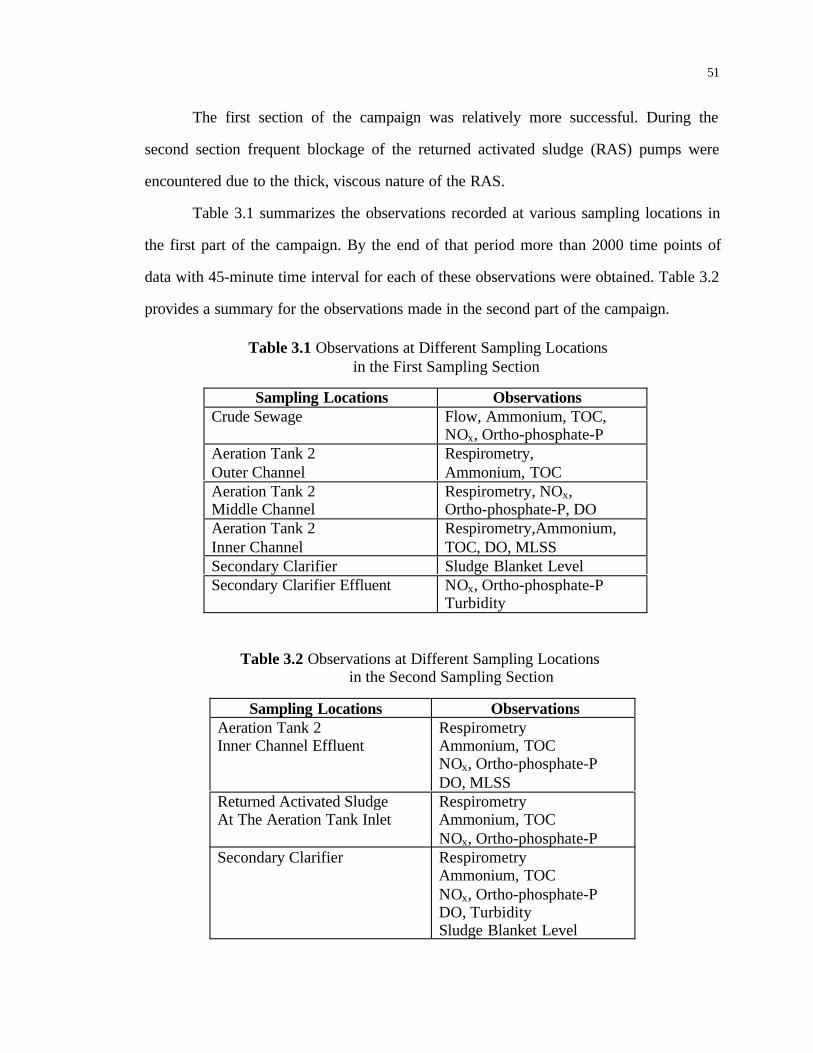
51
The first section of the campaign was relatively more successful. During the
second section frequent blockage of the returned activated sludge (RAS) pumps were
encountered due to the thick, viscous nature of the RAS.
Table 3.1 summarizes the observations recorded at various sampling locations in
the first part of the campaign. By the end of that period more than 2000 time points of
data with 45-minute time interval for each of these observations were obtained. Table 3.2
provides a summary for the observations made in the second part of the campaign.
Table 3.1 Observations at Different Sampling Locations in the First Sampling Section
Sampling Locations ObservationsCrude Sewage Flow, Ammonium, TOC,
NOx, Ortho-phosphate-PAeration Tank 2Outer Channel
Respirometry,Ammonium, TOC
Aeration Tank 2Middle Channel
Respirometry, NOx,Ortho-phosphate-P, DO
Aeration Tank 2Inner Channel
Respirometry,Ammonium,TOC, DO, MLSS
Secondary Clarifier Sludge Blanket LevelSecondary Clarifier Effluent NOx, Ortho-phosphate-P
Turbidity
Table 3.2 Observations at Different Sampling Locations in the Second Sampling Section
Sampling Locations ObservationsAeration Tank 2Inner Channel Effluent
RespirometryAmmonium, TOCNOx, Ortho-phosphate-PDO, MLSS
Returned Activated SludgeAt The Aeration Tank Inlet
RespirometryAmmonium, TOCNOx, Ortho-phosphate-P
Secondary Clarifier RespirometryAmmonium, TOCNOx, Ortho-phosphate-PDO, TurbiditySludge Blanket Level

52
3.3 ENVIRONMENTAL PROCESS CONTROL LABORATORY (EPCL)
3.3.1 Introduction
The Environmental Process Control Laboratory (EPCL) was manufactured by
Capital Controls (Minworth Systems Limited) in Birmingham, England. It can be used in
many contexts, especially in the study of municipal and industrial wastewater treatment,
protection of surface water quality, and groundwater contamination. It is also referred to
as being “mobile” in the sense that it can be moved around and deployed at different sites
for real-time water quality monitoring as opposed to an ordinary “stationary” laboratory
in a building. In this research the EPCL was fully adopted to support the development of
a dynamic process model for the activated sludge system at the Athens Wastewater
Treatment Facility No. 2 in Athens, GA.
3.3.2 Hardware Aspects
As seen in Figure 3.5, the two white trailers essentially comprise the so-called
Environmental Process Control Laboratory (EPCL). Each of the trailers is equipped with
on-line automatic monitors. One trailer houses a respirometer, ammonium monitor, TOC
monitor, and turbidity sensor (specifically for determining samples with low suspended
solid concentrations, such as secondary clarifier effluent) coupled with a homogenizer
and a debubbler. The other trailer has a respirometer, NOx (nitrite and nitrate) monitor
and orthophosphate monitor. Figure 3.6 presents the interior view of the trailer. Other
than the on-board monitors, such out-board monitors as two DO probes, a mixed liquor
suspended solid (MLSS) probe, and a sludge blanket level sensor are installed outside the
trailers in the process tanks. For instance, the sludge blanket level sensor was fixed to the
bridge over the secondary clarifier to monitor the movement of sludge blanket level.
Most of these monitors have the capability of self-cleaning and self-calibration
operations. The calibration frequency is preset by the commands issued at the “Trailer

53
Terminal” interface, which is explained below. Some monitors, such as DO probes, can
even perform the function of self-correction, which is to correct its operation against
driftings or malfunctions. The following is brief definitions of the monitors in the EPCL,
their corresponding analytical methods and the calibration frequency against the
standards (where appropriate).
Figure 3.5 External View of the EPCL
Figure 3.6 Internal View of the EPCL

54
Each on-board and out-board monitor will be defined in summary note form as follows.
On-board Monitors
q Respirometer
In tank form designed by Capital Controls (MSL), housing the following monitors
with their respective working ranges: temperature (0-50oC); pH (0-14); DO (0-10gm-
3); MLSS (0-10,000gm-3); and conductivity (0-20,000µS).
q Ammonium Monitor
Designed by Capital Controls (MSL) with heat-insulated, temperature-controlled
housing, ion-selective probe (a Cole Palmer 27502-00 gas sensing electrode), and a
pH probe for monitoring the pH of a caustic buffer together with a temperature
sensor. Operating range is 0-100gm-3, with daily calibration against 1gm-3 and 10gm-3
standard solutions.
q TOC Monitor
Pollution and Process Monitoring Protoc 100 TOC analyzer using and infra-red CO2
detector (0-3,000ppm) to provide an operating range of 0-500gm-3 TOC. Calibration
is on a daily basis using clean water and a standard solution of 200gm-3 TOC.
q Orthophosphate Monitor
Designed by Capital Controls (MSL) using colorimetric detection and having an
operating range of 0-20gm-3; calibration is on a daily basis using a combination of an
obscured light source, an empty cell, and a standard solution of 10gm-3
orthophosphate.
q Nitrate/TON (NOx) Monitor
Prototype Capital Controls (MSL) design using colorimetric detection of NO2 and 0-
30gm-3 TON. Calibration is on a daily basis using a combination of an obscured light
55
source, an empty cell, and a standard solution of 10gm-3 TON made up of 90% nitrate
and 10% nitrite.
q Turbidity Sensor
Infra-red reflection (Nephelometric) detection operating over 0-500ftu ranges and
designed by Capital Controls (MSL). Calibration is done manually.
Out-board Monitors
q Sludge Blanket Level Sensor
Zellweger Analytics SLM-3000 sludge level monitor and profiler with 4-way
detector.
q DO Probe
Clarke-type DO cell designed by Capital Controls (MSL), with Danfoss Evita
085G0022 DO cartridge. The probe is pneumatically operated, self-cleaning and self-
calibrating against air in the respirometer and against air blown into the housing on a
daily basis.
q MLSS Probe
Optical detection system designed by Capital Controls (MSL), pneumatically
operated and self-cleaning. Requires manual calibration against either a formazin
standard, clean water, or gravimetric analysis of grab samples of sludge on a daily
basis.
Each of the trailers can continuously receive samples from three locations on site.
All the samples are pretreated through the ultrafilters to ensure being solid-free before
being presented to the instrumentations on-board. Filtrates from these ultrafilters enter
each individual monitor in turn through pneumatical valves. For instance, the ammonium
monitor is presented in turn with a sample from each of the three streams, producing a

56
measurement of the ammonium concentration in each of the three sample lines once
every 45 minutes.
Day-to-day records of all measurements taken in 15-minute sampling interval are
stored in the on-board data loggers, together with data recorded with a much shorter time
interval down to one second. The data with much shorter time intervals are essentially
electrical signals gathered during the calibration cycles of each instrument for diagnostic
purposes. Since the data logger can only hold a data volume of up to several days, the
on-line data amassed are accordingly transferred from the local system to a remote UNIX
based workstation through a phone line on a regular basis.
In order to check the operational status or set up the operational mode of the
monitors, the instruments can be accessed in three ways:
q Front panel access, which is for access to the operational information of the
instruments with the keypads on the faces of the instruments;
q Local PC access, which is to hook up a personal PC to the communication port on-
board such that the operational information of the instruments can be assessed and/or
changed with one of the three-letter commands;
q Remote PC access, which is to remotely check or reset the operational information of
the instruments through a phone line without even being in the EPCL in person.
3.3.3 Software Aspects
The software package of the EPCL has the following components:
q FT for windows (Capital Controls, 1994)
This enables stored data to be retrieved directly from the monitors, and is usually
used for the purpose of instrument testing.

57
q GFX (Capital Controls, 1996)
This presents the data in graphical form. It can also export data in a format
compatible with the "Translate for Windows" program, which makes it possible to
add or edit "GFX for Windows" data.
q Translation for Windows (Capital Controls, 1996)
This allows a file with time-stamped data to be converted into a form where it is
manipulated by GFX. It is designed to facilitate viewing and limited editing of the
data.
q Trailer Terminal (Capital Controls, 1996)
This provides a platform for accessing and controlling the operations of the
instrumentations.
3.3.4 Quality Assurance and Quality Control (QA/QC)
The detailed data files logged at a resolution of down to 1-second intervals are
collected principally for QA/QC purposes. Whenever a monitor is engaged in a self-
calibration, a detailed data file is triggered with diagnostic information being logged. By
checking the diagnostic information of an individual monitor, a judgement can be made
as to whether the monitor is functioning properly, or otherwise identify possible
problems. For example, the measurements taken by the orthophosphate monitor involve a
colorimetric mechanism. Figure 3.7 shows the PO4 Head Output curve when the
orthophosphate monitor is functioning properly, while the curve as seen in Figure 3.8
denotes problems with the monitor. The PO4 Head Output is the voltage generated by the
amplifier and thus is an easy indicator of the proper functioning of the monitor. In Figure
3.8 there is none of the color development phase as seen in Figure 3.7 (the flat platform
near the tail end of the curve), which is caused by reagent failure, either because of
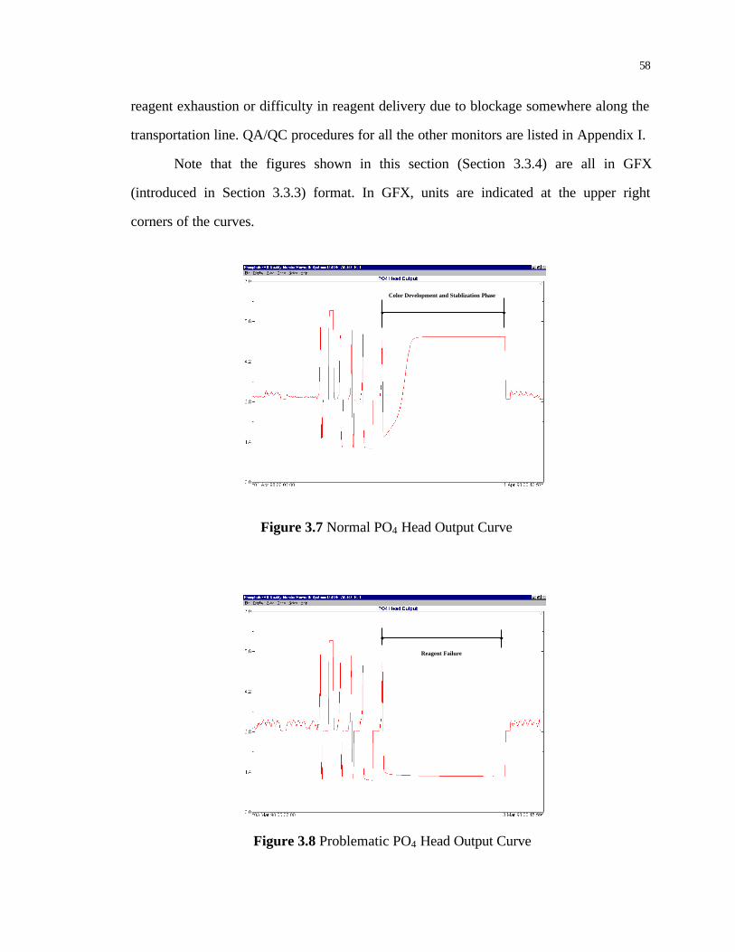
58
reagent exhaustion or difficulty in reagent delivery due to blockage somewhere along the
transportation line. QA/QC procedures for all the other monitors are listed in Appendix I.
Note that the figures shown in this section (Section 3.3.4) are all in GFX
(introduced in Section 3.3.3) format. In GFX, units are indicated at the upper right
corners of the curves.
Figure 3.7 Normal PO4 Head Output Curve
Figure 3.8 Problematic PO4 Head Output Curve
Reagent Failure
Color Development and Stablization Phase

59
Regular intra- and inter-laboratory checking of the standard solutions for the
monitors is also essential for ensuring quality of the data quality. Using again the
example of the orthophosphate monitor, it gave a reading of 10.00mg/L to a 10mg/L
standard solution. The standard solution was also sent to the on-site laboratory at the
Athens Wastewater Treatment Facility No.2 for inter-laboratory checking, where the
result was 10.13mg/L.
3.3.5 Practical Experience With The On-line Monitors
The on-line monitors require attentive service and maintenance if they are to
function properly. A complete daily routine was consistently exercised during the
sampling campaign to ensure smooth operation of the EPCL. This daily routine basically
included checking instrument status through the built-in software and visual inspection.
Checking logged diagnostic data for each monitor with the EPCL built-in software allows
one to determine the possibility of existing problems, such as those indicated in Figure
3.8 for the orthophosphate monitor. A summary of the daily maintenance checklist is
included in Appendix II.
Typical of the raw time-series is that for ammonium concentration in the crude
sewage shown in Figure 3.9. The abrupt decrease of ammonium concentration labeled as
1 was caused by the misplacement of the sodium hydroxide suction tube. Sodium
hydroxide is used for the ammonium monitor to maintain an ideal alkalinity. After the
normal NaOH transport into the ammonium monitor was recovered, the diagnostic curve
returned to a “normal” value. On some occasions the ammonium monitor failed due to a
faulty ammonia probe, in which case the voltage output of the probe was extremely low
compared to the desired, optimum value. In order to overcome this kind of problem, the
ammonia probe was replaced, and the monitor was recalibrated and left to stabilize for at
least 24 hours before the normal measurement was resumed. Generally, after replacement
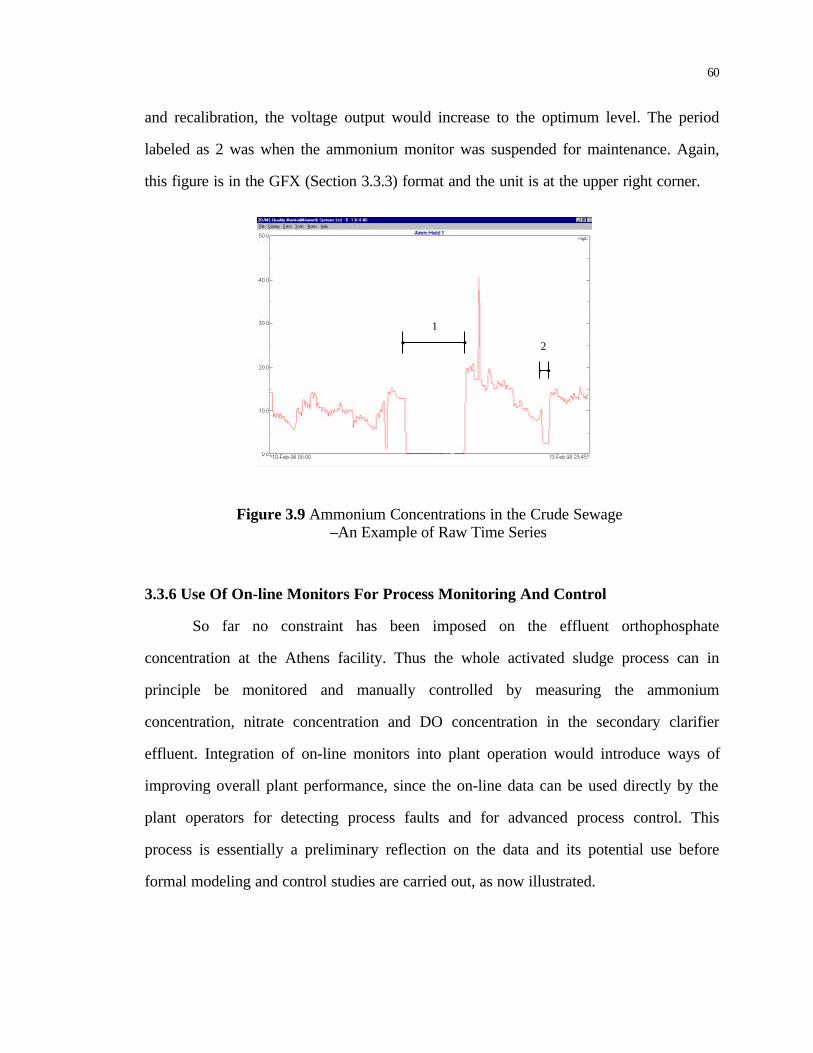
60
and recalibration, the voltage output would increase to the optimum level. The period
labeled as 2 was when the ammonium monitor was suspended for maintenance. Again,
this figure is in the GFX (Section 3.3.3) format and the unit is at the upper right corner.
Figure 3.9 Ammonium Concentrations in the Crude Sewage –An Example of Raw Time Series
3.3.6 Use Of On-line Monitors For Process Monitoring And Control
So far no constraint has been imposed on the effluent orthophosphate
concentration at the Athens facility. Thus the whole activated sludge process can in
principle be monitored and manually controlled by measuring the ammonium
concentration, nitrate concentration and DO concentration in the secondary clarifier
effluent. Integration of on-line monitors into plant operation would introduce ways of
improving overall plant performance, since the on-line data can be used directly by the
plant operators for detecting process faults and for advanced process control. This
process is essentially a preliminary reflection on the data and its potential use before
formal modeling and control studies are carried out, as now illustrated.
1
2

61
Use of On-line Monitors for Process Fault Detection
The activated sludge process requires a thorough control of the dissolved oxygen
concentrations in the aeration tanks. It is important to sustain a given dissolved oxygen
level for efficient nitrification and reasonable energy consumption. However, during the
period of Figure 3.10, dissolved oxygen concentration in the middle channel (lower plot)
was consistently deficient compared to dissolved oxygen concentration in the inner
channel (upper plot).
Figure 3.10 Dissolved Oxygen Concentration in (a) the Inner channel and (b) Middle Channel (bottom) of Aeration Tank #2.
In order to obtain complete nitrification, ammonium in the crude sewage has to be
oxidized to nitrite and eventually to the end product of nitrate. However, during the time
period from 5 February, 1998 to 5 April, 1998, there was an obvious ammonium buildup
in both the outer channel and inner channel of aeration tank #2, and correspondingly loss
of nitrification in terms of nitrite and nitrate decreases in the middle channel and clarifier
effluent (See Figure 3.11). In Figure 3.11 the plots in the left column are in the sequence
of ammonium concentration in the outer channel, and nitrite and TON concentrations in
(a)
(b)
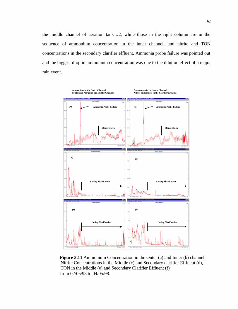
62
the middle channel of aeration tank #2, while those in the right column are in the
sequence of ammonium concentration in the inner channel, and nitrite and TON
concentrations in the secondary clarifier effluent. Ammonia probe failure was pointed out
and the biggest drop in ammonium concentration was due to the dilution effect of a major
rain event.
Ammonia Probe Failure Ammonia Probe Failure
Major Storm Major Storm
Ammonium in the Outer Channel Nitrite and Nitrate in the Middle Channel
Losing Nitrification Losing Nitrification
Losing Nitrification Losing Nitrification
Ammonium in the Inner Channel Nitrite and Nitrate in the Clarifier Effluent
(a) (b)
(c)(d)
(e) (f)
Figure 3.11 Ammonium Concentration in the Outer (a) and Inner (b) channel, Nitrite Concentrations in the Middle (c) and Secondary clarifier Effluent (d), TON in the Middle (e) and Secondary Clarifier Effluent (f) from 02/05/98 to 04/05/98.

63
Use of On-line Monitors for Process Control
During heavy rain events, the high flow rate to the plant leads to high
concentrations of suspended solids in the secondary clarifier effluent.
Figure 3.12 (a) Influent Flow, (b) MLSS In Inner Channel of Aeration Tank #2, (c) Sludge Blanket Level, and (d) Secondary Effluent Suspended Solids Concentration During One of the Rain Events.
Figure 3.12 shows the wastewater flow, the MLSS concentration in the inner
channel of aeration tank No.2, the sludge blanket level in one of the secondary clarifiers,
and the suspended solids concentration in the effluent of one of the secondary clarifiers
during a major rain event. The figure shows that the influent flow jumped to over
1300m3/h from an average 800m3/h, thus diluting the mixed liquor concentration in the
aeration tank. The sludge blanket level increased on this occasion with a time delay due
to transport reason, causing heavy sludge loss with the effluent. In cases of this kind the
plant adopted alternative strategies. The process control action taken then was that the
Major Storm
Mixed Liquor Concentration Secondary Clarifier Effluent Suspended Solids Concentration
Operational Mistake
Sample LineOff
Manual Calibration
(a)
(b)
(c)
(d)
Dilution Effect of the Storm
Sludge Blanket LevelIncrease due to the Storm
Sludge Loss
Minor Storm
Sludge Loss

64
influent was directed to the inner channel of the aeration tank, bypassing the first two.
The returned activated sludge, however, still went through regular route, that is, from
outer channel through middle channel to inner channel. But its rate was much slower than
under “normal weather” condition. Influent flow was switched back to the outer channel
when it fell to a normal level.
Aspects of process control, including sludge age control, feedback control of
return sludge rate and sludge wastage rate, step feed, step sludge, and DO set-point
control, will be experimented fully in Chapter 6.
3.4 INTRODUCTION TO SMOOTHING ALGORITHM OF TVP ANALYSIS
TOOLBOX
Great efforts were made to make sure that the sampling process was carried out
as smooth as possible, as described in the previous sections in this Chapter. However,
things still went wrong in spite of these efforts. The ammonium probe failed; the sample
line became blocked; a switch was left in the “off” position after manual maintenance of
an instrument; a lawn-mower destroyed one of the sample lines by driving over it; and so
on. These factors result in gaps, drift, and potential outliers in the retrieved data sets.
Their corrupting effects have to be accounted for before the raw data are presented for
development and evaluation of the mathematical model in Chapters 4 and 5. The goal is
to generate a set of refined, clean data, yet without tainting them in the process. Among
the many approaches available for signal pre-processing, our work has employed a
package of software constructed around the algorithms of recursive estimation and time-
series analysis (Young, 1984; Young and Benner, 1991), in particular, a smoothing
algorithm based on filtering theory, as illustrated through applications in processing
hydrological data in Young and Beven (1994) and Young et. al., (1997).
65
This software is based on a Kalman filter, and processes the time-series data first
forwards and then backwards in time. Smoothed estimates of the components of the
observed signal, typically its long-term trend and seasonal components, are therefore
generated at each point in time with the benefit of having processed the entire record of
the data. The net effect of this is to give the software the ability to deal successfully with
outliers and to interpolate across gaps in the data (Beck and Liu, 1999). Interpolation
across the gaps in the model input data stream is especially important for implementing a
model, since these are the forces driving the model and must be given for each period of
the solution scheme.
3.5 EXAMPLE OF SMOOTHED MODEL INPUT DATA
Using ammonium concentration in the crude sewage as an example, the
procedures taken to obtain the trend, seasonal component, and smoothed traces of the raw
data with a so-called Dynamic Harmonic Regression (DHR) algorithm in the Time
Variable Parameter (TVP) toolbox are summarized as follows.
The basic DHR model contains trend, seasonal, cyclical, and white noise
components: i.e.,
ttttt eCSTy +++= t = 1, 2, …, N (3.1)
where,
St–Seasonal component;
Ct–Cyclical component;
Tt–Trend;
et–White noise.

66
The seasonal component is described as:
∑=
+=i
itiitit tbtaS1
,, )}sin()cos({ ωω (3.2)
where,
ai,t and bi,t–Stochastic time variable parameters (TVP’s);
ωi (i=1,2,…,Rs)–Fundamental and harmonic frequencies associated with the seasonality.
The cyclical component is described as:
∑=
+=i
itiitit tftfC1
,, )}sin()cos({ βα (3.3)
where,
αi,t and β i,t–Stochastic time variable parameters (TVP’s);
fi (i=1,2,…,Rc)–Fundamental and harmonic frequencies associated with the cyclical
component.
In the TVP analysis toolbox, however, the cyclical component is not taken into
account. Therefore, the DHR model is simplified into the following format:
tttt eSTy ++= t = 1, 2, …, N (3.4)
In order to specify an appropriate form of equation (3.4) for a specific data stream, it is
necessary to identify the number and values of the fundamental and harmonic frequencies
associated with the seasonality in equation (3.2). This is accomplished by referring to the
empirical spectral properties of yt in equation (3.4) using standard methods of spectral
analysis (Priestley, 1981). There are many ways to compute the empirical spectrum, but
one of the most useful is the Auto Regression (AR) spectrum of the data, with the AR
order identified from the Akaike Information Criterion (AIC) (Priestley, 1981). The AR
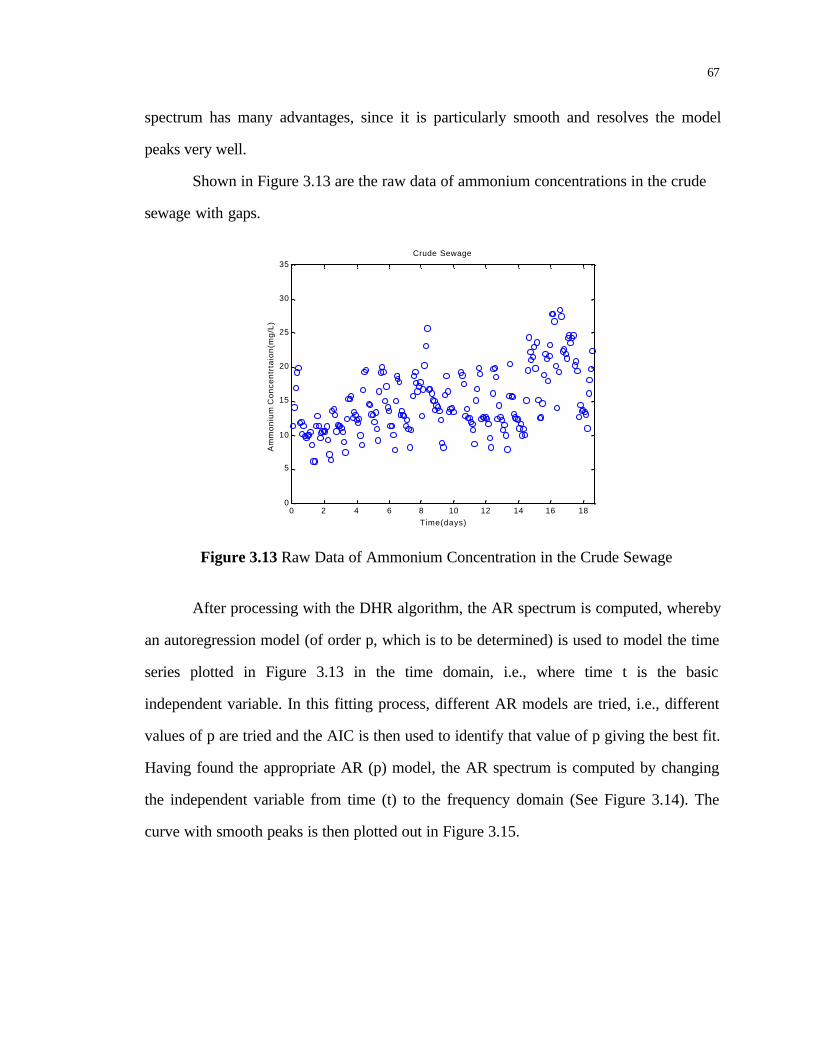
67
spectrum has many advantages, since it is particularly smooth and resolves the model
peaks very well.
Shown in Figure 3.13 are the raw data of ammonium concentrations in the crude
sewage with gaps.
0 2 4 6 8 10 12 14 16 180
5
10
15
20
25
30
35
Time(days)
Am
mo
niu
m C
on
cen
trta
ion
(mg
/L)
Crude Sewage
Figure 3.13 Raw Data of Ammonium Concentration in the Crude Sewage
After processing with the DHR algorithm, the AR spectrum is computed, whereby
an autoregression model (of order p, which is to be determined) is used to model the time
series plotted in Figure 3.13 in the time domain, i.e., where time t is the basic
independent variable. In this fitting process, different AR models are tried, i.e., different
values of p are tried and the AIC is then used to identify that value of p giving the best fit.
Having found the appropriate AR (p) model, the AR spectrum is computed by changing
the independent variable from time (t) to the frequency domain (See Figure 3.14). The
curve with smooth peaks is then plotted out in Figure 3.15.

68
Figure 3.14 AR Spectrum of Order 16 for Ammonium Concentration in the Crude Sewage
0 2 4 6 8 10 12 14 16 180
5
10
15
20
25
30
35
Time(days)
Am
mo
niu
m C
on
cen
trta
ion
(mg
/L)
Crude Sewage
raw data smoothed data
Figure 3.15 Raw and Smoothed Data of Ammonium Concentration in the Crude Sewage
20 10 6.67 5 4 3.33 2.86 2.5 2.22
0
0.5
1
1.5
2
2.5
3
3.5
4
AR(16) Spectrum of Ammonium Concentration in the Crude Sewage
Period(samples/cycle)
log1
0(P)
Fitted ARSpectrum
Actual ARSpectrum

69
From the AR spectrum curve in the frequency domain, the number of
fundamental and harmonic components can be specified. Thus the overall structure of the
DHR model can be determined, i.e., the choice of Rs in equation (3.2).
0 2 4 6 8 10 12 14 16 180
5
10
15
20
25
30
35
Time(days)
Am
mo
niu
m C
on
cen
trta
ion
(mg
/L)
Crude Sewage
raw datatrend
Figure 3.16 Raw Data of Ammonium Concentration in the Crude Sewage and its Trend
0 2 4 6 8 10 12 14 16 18-10
-8
-6
-4
-2
0
2
4
6
8
10
Time(days)
Am
mo
niu
m C
on
cen
trta
ion
(mg
/L)
Crude Sewage
Figure 3.17 Seasonal Component of Ammonium Concentration in the Crude Sewage

70
Therefore, the variations of the DHR model’s component parameters over time
can be estimated, which then generates the trend and diurnal oscillation curves as shown
in Figure 3.16 and Figure 3.17.
Either of the two different traces for ammonium concentration in the crude
sewage with the gaps filled can possibly be used as model input data stream. One trace is
the pure smoothed data produced from the DHR algorithm (the curve plotted as a
continuous line in Figure 3.15. The other option is the raw data with its gaps filled with
data produced from the DHR algorithm. Table 3.3 illustrates the difference between these
two different model input traces using some numbers from the observed sequence. The
effect of these two different input traces for ammonium concentration in the crude
sewage on the simulation results of ammonium concentration in the inner channel is
plotted out in Figure 3.18.
Table 3.3 Difference of Two Model Input Traces
Raw Data with Gaps
Smoothed Data from DHR Analysis
Raw Data with Gaps Filledwith Data from DHR Analysis
1.5 1.3 1.52 1.8 2
3.1 3.2 3.1NaN 3.4 3.4NaN 3.6 3.64.3 4.3 4.33.7 3.4 3.75 4.8 5
4.4 4.1 4.44 3.9 4
3.9 3.6 3.93.8 3.5 3.8
NaN 3.6 3.63.5 3 3.54 3.7 4
In Table 3.3, “NaN” denotes gap in the raw data stream.

71
0 2 4 6 8 10 12 14 16 180
2
4
6
8
10
12
14
16
18
20
22
Time(days)
Am
mo
niu
m C
on
cen
trta
ion
(mg
/L)
Crude Sewage
raw data with gaps smoothed data simulation result with smoothed data simulation result with gaps in raw data filled with DHR result
Figure 3.18 Comparison of Model Result of Ammonium Concentration in the Inner Channel with Different Model Input Streams
In Figure 3.18 the sequence plotted in circle is the raw data of ammonium
concentration in the inner channel corrupted with gaps, and the sequence plotted in
diamonds is the smoothed data of ammonium concentration in the inner channel without
gaps. The curve plotted in red line is the model simulation result of ammonium
concentration in the inner channel with smoothed ammonium concentration in the crude
sewage as model input, while the curve plotted in blue line is the model simulation result
of ammonium concentration in the inner channel with raw ammonium concentration in
the crude sewage plus gaps filled with data produced from DHR analysis as model input.
There is little difference between the two model simulation results, but the trace in
circles, i.e., raw ammonium concentration in the inner channel data with gaps, provides a
better model fitting result. So what can be concluded from this exercise is that using raw

72
data with gaps filled with data produced from DHR algorithm as model input is a
reasonable way to pre-process the raw data streams and it does a better job in allowing us
to reconcile the model with the data.
Other than smoothing the raw data set, worthy of mention in passing is the
potential of the TVP toolbox in assessing transport and mixing properties of both solute
and particulate materials as they pass through the bioreactor and secondary clarifier of the
activated sludge process. This can be achieved through identifying Active Mixing
Volume (AMV) models (Young and Lees, 1993) using the seasonal components
extracted from the same variable, such as ammonium-N, at different sampling locations.
3.6 CONCLUSIONS
This Chapter describes how high quality data was collected in the case study at
Athens Wastewater Treatment Facility No.2, and how the resulting data streams are pre-
processed without bias by the so-called “TVP analysis toolbox” before being presented
for model development in the next Chapter.
The scope and quality of the data retrieved from Athens Wastewater Treatment
Facility No.2 with EPCL are found to be better than what have been presented in the key
published papers mentioned in Chapter 2 (Bliss et al., 1986; Siegrist et al., 1992; Ducato
et al., 1995; Carlsson et al., 1996; Rouleau et al., 1997).
73
CHAPTER 4
MODEL DEVELOPMENT
4.1 INTRODUCTION
This chapter is organized as follows. The purposes for which the model is to be
developed are stated first in section 4.2. Following a brief statement of the overall
structure of the model (section 4.3), section 4.4 sets out the key modification of the
aerator sub-model with respect to characterization of solute and particulate transport. The
clarification and thickening functions of the secondary clarifier model are discussed in
section 4.5. A key assumption is that all particulate matter entering the settler from the
aerator passes into the thickening zone of the model. Any suspended solids subsequently
found in the clarification zone are represented by an upward flux at the interface between
the thickening and clarification zones. Discussion of the features of the model is given in
section 4.6.
4.2 PURPOSE OF THE MODEL
The model should be able to simulate general behavior of the wastewater
treatment plant, i.e., carbonaceous oxidation, nitrification, denitrification, and ortho-
phosphate-P removal. To satisfy the above objectives, it is unavoidable that a large
dynamic model will have to be developed. Such a model would apparently be undesirable
because of its lack of identifiability (Beck, 1987). However, the model is to be used as a
test bed for the development of control strategies. As with any model, the model is
inevitably a simplification of highly complex kinetic processes. Despite the uncertainty
surrounding many of the mechanisms in the model (Chen, 1993), such a model will be
acceptable as long as the sensitivity of the control strategies to such uncertainty can be

74
established. In other words, if we can find a control strategy that works well irrespective
of the gross uncertainty attaching to the model, using such a large model is legitimate.
In the following sections, a dynamic multiple-species model is thus developed in
order to meet the above objective. In Chapter 5 the model’s parameters are established
with reference to field data. “Trial-and-error” calibration is adopted for this case study. In
Chapter 6, the calibrated model is subsequently used for the assessment of control
strategies to explore the extent to which such a capability could improve process
performance.
4.3 OVERALL ARRANGEMENT OF THE MODEL
Generally speaking, the model contains three independent sub-models according
to their functions in the whole system. The aerator is where the various biological
reactions take place. The thickener is where the biomass is concentrated and then
recycled back to the reactor/aerator. The clarification zone is where solid/liquid
separation takes place.
The thickening and clarification functions occur within the secondary clarifier.
The arrangement of the sub-models is shown in Figure 4.1. The state variables for each
sub-model, as well as their inputs, are listed in Table 4.1. Input variables except return
sludge flow and wastage sludge flow rates were monitored by the EPCL in a continuous
manner at the Athens Wastewater Treatment Facility No.2. Return sludge flow and
wastage flow rates were monitored on a daily basis by the plant. All the sub-models are
predominantly “mechanistic” in nature. The parameters associated with these
mechanisms are summarized in Table 4.2. In Figure 4.1, “XA” represents the aeration
tank; “XB1” represents the thickening zone; “XB2” represents the compaction zone;
“XC” represents the clarification zone.

75
Figure 4.1. Schematic Structure of the Activated Sludge Model
Table 4.1 Definitions of State Variables and Input Variables in the Activated Sludge Model
Variable DefinitionXAi,j
XB1i,s andXB2i,s
State variables in the ith CSTR of the aerator sub-modelj=1 Ammonium (SNH4)
2 Nitrosomonas (XSO)3 Nitrite (SNO2)4 Nitrate (SNO3)5 Nitrobacter (Xba)6 Easily biodegradable substance (Seasy)7 Fermentation products (Sferment)8 Heterotroph (XH)9 Slowly biodegradable substance (Xslow)10 Ortho-phosphate-P (SPO4)11 Phosphorus-accumulating bacteria (XPAO)12 Cell internal organic storage substance (XPHA)13 Poly-P (XPP)14 Dissolved oxygen (SO2)15 Mixed Liquor Suspended Solids (XMLSS)
State variables in the ith CSTR of the thickening zone sub-model and in the compaction zone sub-model respectivelys=1 SS (XSS)
2 Ammonium (SNH4)3 Nitrite (SNO2)4 Nitrate (SNO3)
Aerator XA Thickener
Clarification Zone XC
Effluent
Returned SludgeWasted Sludge
Thickening Zone (XB1)
Compaction Zone (XB2)
CrudeSewage
Secondary Clarifier

76
XCi,s
Um
UCk
V1V2V3
ASCAaHCiHSBi
HCZHSBM
5 Easily biodegradable substance (Seasy)6 Fermentation products (Sferment)7. Slowly biodegradable substance (Xslow)8. Ortho-phosphate-P (SPO4)
State variables in the ith CSTR of the clarification zone sub-models=1 SS (XSS)
2 Ammonium (SNH4)3. Nitrite (SNO2)4. Nitrate (SNO3)5. Easily biodegradable substance (Seasy)6. Fermentation products (Sferment)7. Slowly biodegradable substance (Xslow)8. Orthophosphate-P (SPO4)
Measured input variablesm=1 Influent flow (QI)
2 Returned activated sludge flow (QR)3 Wasted sludge flow (QW)4 Influent ammonium (SNH4)5 Influent nitrite (SNO2)6 Influent nitrate (SNO3)7 Influent total organic carbon (STOC)8 Influent ortho-phosphate-P (SPO4)Note: no measurement of input DO concentration isavailable.
Input variables to the secondary clarifier, k has the samemeaning as in XCi,s
Volume of water in the outer channel of the aeration tankVolume of water in the middle channel of the aeration tankVolume of water in the inner channel of the aeration tankCross sectional area of the secondary clarifierCross sectional area of the aeration tankHeight of the ith CSTR of the clarification zoneHeight of the ith CSTR of the thickening zone other than thetop oneHeight of the compaction zoneHeight of the top CSTR in the thickening zoneNote: HCi, HSBi, and HSBM are time-varying. While Hcz is
fixed.
In this table, CSTR represents Continuously Stirred Tank Reactor.

77
Table 4.2 Parameters in the Activated Sludge Model
Symbols Definitionmax_vel
paravel
alpha1
alpha2 & cratio1
ratio2
ratio3
beta
alpha45
alpha46alpha54
KO2_SO, KO2_ba
KO2_H, KO2_PAOa2b2b1YSO
Yba
YhYPAO
bso
bbabhbPAO
bPHA
bPP
Settling velocity of suspended solids in thethickening zone (feet/h)Settling parameter (l/mg)Settling velocity of suspended solids from top CSTRto bottom CSTR in the aeration tank (feet/h)Ratio of Qabove/(QI+QR) in the aeration tank, whereQabove is the flow through the upper layer CSTRs inthe aeration tank (%)Parameters in QResuspension=alpha2*(QI+QR)^cFraction of active volume in the outer channel of theaeration tank (%)Fraction of active volume in the middle channel ofthe aeration tank (%)Fraction of active volume in the inner channel of theaeration tank (%)Fraction of RAS flow dropping into the 1st bottomCSTR upon entering the aeration tank due to thedensity difference between water and sludge (%)Minimum flux from the thickening zone to theclarification zone (mg/l)Resuspension factor(d/MG)Settling velocity of solids in the clarification zone ofthe secondary clarifier (feet/h)Saturation coefficients for oxygen (mg O2/l)
Biomass growth factor in the bottom CSTRs (d-1)Biomass decay factor in the bottom CSTRs (d-1)Biomass decay factor in the upper CSTRs (d-1)Yield coefficient for Nitrosomonas (g Nitrosomonasformed/g NH4 oxidized)Yield coefficient for Nitrobacter (g Nitrobacterformed/g NO2 oxidized)Yield coefficient for heterotroph (g/g)Yield coefficient for phosphorus-accumulatingbacteria (g PAO formed/g PHA)Decay coefficient for Nitrosomonas (d-1)Decay coefficient for Nitrobacter (d-1)Decay coefficient for heterotroph (d-1)Decay coefficient for phosphorus-accumulatingbacteria (d-1)Rate constant for lysis of cell internal organic storagesubstance (d-1)Rate constant for lysis of poly-P (d-1)

78
qppqpha
ipbmKNH4_SO
KNO2_ba
KPO4_SO
KPO4_ba
Keasy_h
KNO3_h
KNH4_h
Kpo4_h
KNO2_h
fxiKh
Kx_h
qfe
eda_NO3
Kfe
KNH4_PAO
Keasy_PAO
KPO4_PAO
KNO3_PAO
KA_PAO
KPP
KPHA
Kmax
Kipp
Rate constant for storage of poly-P (d-1)Rate constant for storage of cell internal organicstorage substance (d-1)Phosphorus content of biomassSaturation constant of ammonium for Nitrosomonas(mg NH4/l)Saturation constant of nitrite for Nitrobacter (mgNO2/l)Saturation constant of phosphorus for Nitrosomonas(mg P/l)Saturation constant of phosphorus for Nitrobacter(mg P/l)Saturation constant of easily biodegradable substancefor heterotroph (mg/l)Saturation constant of nitrate for heterotroph (mg/l)Saturation constant of ammonium for heterotroph(mg/l)Saturation constant of phosphorus for heterotroph(mg P/l)Saturation constant of nitrite for heterotroph (mg/l)Fraction of inert substance in biomass lysisRate constant of hydrolysis (d-1)Saturation constant for slowly biodegradablesubstanceMaximum fermentation rate (d-1)Anoxic hydrolysis reduction factorSaturation coefficient for fermentation of easilybiodegradable substance (mg/l)Saturation constant of ammonium for phosphorus-accumulating bacteria (mg/l)Saturation constant of easily biodegradable substancefor phosphorus-accumulating bacteria (mg/l)Saturation constant of phosphorus for phosphorus-accumulating bacteria (mg P/l)Saturation constant of nitrate for phosphorus-accumulating bacteria (mg N/l)Saturation constant of fermentation product forphosphorus-accumulating bacteria (mg/l)Saturation constant of poly-P for phosphorus-accumulating bacteria (mg PP/mg PAO)Saturation constant of cell internal storage organicsubstance for phosphorus-accumulating bacteria (mgPHA/mg PAO)Maximum ratio of Poly-P/phosphorus-accumulatingbacteria (mg PP/mg PAO)Inhibition coefficient for poly-P storage (mg PP/mg
79
constgamma_PO4
gamma_pha
ratio_so
ratio_ba
ratio_h
ratio_pao
ratio_pha
ratio_ppratio_slowdeni1
deni2
deni3
deni4
percentage_easypercentage_fermentpercentage_inertmiu_somiu_bamiu_hmiu_pao
PAO)Oxygen transfer coefficient (d-1)Poly-P requirement per cell internal storage organicsubstance stored (g P/g)Cell internal storage organic substance requirementfor poly-P storage (g/g)Ratio of Nitrosomonas in the returned activatedsludge (%)Ratio of Nitrobacter in the returned activated sludge(%)Ratio of heterotroph in the returned activated sludge(%)Ratio of phosphorus-accumulating bacteria in thereturned activated sludge (%)Ratio of cell internal storage organic substance in thereturned activated sludge (%)Ratio of poly-P in the returned activated sludge (%)Ratio of slowly biodegradable substance (%)Denitrification rate of nitrite in the upper CSTRs ofall three channels (d-1)Denitrification rate of nitrate in the upper CSTRs ofall three channels (d-1)Denitrification rate of nitrite in the bottom CSTRs ofall three channels (d-1)Denitrification rate of nitrate in the bottom CSTRs ofall three channels (d-1)Ratio of easily biodegradable substance in TOC (%)Ratio of fermentation products in TOC (%)Ratio of inert substance in TOC (%)Maximum growth rate of Nitrosomonas (d-1)Maximum growth rate of Nitrobacter (d-1)Maximum growth rate of heterotroph (d-1)Maximum growth rate of phosphorus-accumulatingbacteria (d-1)
The reactor sub-model is essentially a modified version of the ASM2 model
(Henze et al., 1986 and 1995a; Lessard, 1989) especially in terms of using a new way to
characterize solute and particulate transport in the activated sludge process. Because of
the interactions between the reactor and the secondary clarifiers, particulate substrates
and various biomass in the reactor outlet have to be aggregated into a single quantity,
mixed liquor suspended solids (MLSS), before they are directed to the secondary

80
clarifier, and then disaggregated into individual parts, i.e., various biomass fractions,
based on their ratios to the total solids (MLSS) before they are transferred back to the
aeration tanks. Detailed discussion of each sub-model now follows.
4.4 AERATOR MODEL STRUCTURE
4.4.1 Conceptual Model Structure
The conceptual structure of the biochemical and microbial interactions in the
aerator model is shown in Figure 4.2.
Figure 4.2 Conceptual Structure of the Biochemical and Microbial Interactions in the Aerator Model
INFLUENT
Ammonium Nitrite Nitrate
Nitrosomonas Nitrobacter O2
Carbonaceous Compounds
Biodegradable Soluble
Biodegradable Particulate
Nonbiodegradable
heterotroph
heterotroph, O2
CO2
Phosphorus Poly-P
PAO, Aerobic
Fermentation Products PHA
No O2
No O2
O2
Biomass Decay
No O2
Energy
No O2
N2 No O2 Carbon
N2
81
Here PAO represents phosphorus-accumulating organisms; Poly-P represents poly-
phosphate, and PHA represents cell internal storage organic substances. Biomass decay
refers to decay of Nitrosomonas, Nitrobacter, heterotroph and phosphorus-accumulating
organisms.
The biochemical processes described in the aerator model as shown in Figure 4.2 are:
q Aerobic growth of autotrophs (Nitrosomonas and Nitrobacter)
q Oxic/anoxic growth of heterotrophs
q Oxic/anoxic growth of phosphorus-accumulating bacteria
q Decay of autotrophs, heterotrophs, and phosphorus-accumulating bacteria
q Oxic/anoxic hydrolysis of slowly biodegradable substances
q Fermentation
q Denitrification from nitrite and nitrate
q Oxic/anoxic storage of poly-P
q Storage of cell internal storage organic substances
q Lysis of cell internal storage organic substances
q Lysis of poly-P.
4.4.2 Solute and Particulate Transport Characterization in the Activated Sludge
Process
The mixing of biomass and nutrients in the aeration tank is normally supposed to
be perfect in the vertical dimension according to conventional activated sludge theory.
However, for an activated sludge system with surface aeration, mechanical mixing may
not be ideal in reality, i.e., partial mixing is achieved at the upper part of the tank with
dead zones created at the lower part of the tank (Nielsen et al., 1999). In other words, the
surface aerators can only mix well a certain amount of mixed liquor (biomass and
nutrients), referred to as the effective mixing volume, such that the rest is left largely
82
unmixed at the bottom of the tank, to which significant amounts of particulate matter may
also settle. From this perspective the contents in the tank are not uniform in concentration
in the vertical direction, so that a two-layer model might better characterize this vertical
variation, which is subsequently confirmed by model simulation results in Chapter 5. The
first step towards the development of this two-layer model is to decompose the three-
dimensional tank into a series of CSTRs in the horizontal based on the channel
configuration. Due to the vertical variation, the physical tank is then divided into layers, a
top and a bottom layer. The volume of each top CSTR is a fraction of the total volume of
the channel to which it belongs, which results in parameters ratio1, ratio2, and ratio3 in
Table 4.2. These three parameters are respectively fractions of active volumes (%) in the
outer, middle, and inner channel of the aeration tank. The flow velocity in the top layer is
significantly higher than that in the bottom layer (Hunze et al., 2000), with alpha1 (as
seen Table 4.2) being the ratio of flow running through the top CSTRs to the combination
of crude sewage and return sludge flows. Crude sewage and returned activated sludge are
separately fed to the top layer of the outer channel of the aeration tank, and the effluent
from the inner channel of the aeration tank leaves the system from the same top layer.
Upon entry into the aeration tank, part of the returned activated sludge, denoted as a ratio
(beta in Table 4.2) of the total amount of return sludge flow, is assumed to drop to the
bottom layer of the outer channel very quickly, as a function of its high density about
10,000 mg/L. Because of hydraulic effects it is assumed that there exist exchanges
between the top layers and the bottom layers immediately below, i.e., upward and
downward fluxes. The upward flow is conceptualized as a linear function (‘alpha2’ in
Table 4.2) of the power (‘c’ in Table 4.2) of the combination of crude sewage and return
sludge (Simons et al., 1992). Conceptually, suspended solids in the top layers undergo
free gravitational settling into the bottom layers immediately below as well, and the

83
settling velocity of suspended solids is described in the same manner as that of Dick and
Young (1972).
The need for separate solute and particulate transport characterization was not
recognized in the first place. In the next Chapter (Chapter 5) the full “story” of how the
changes were made will be explained. The parameters mentioned immediately above in
this section become crucial in making the model fit the data, although we shall have no
hard empirical evidence to assess the “correctness” of the values chosen for them.
The resulting model structure is presented in Figure 4.3.
With the aeration tank being divided into top and bottom layers, it is essentially
assumed that the transport of solute and particulates in the aeration tank now involves
more complicated mechanisms, most notably that the mixed liquor suspended solids
(biomass) cannot be treated, in effect, as a solute. The mathematical counterpart of the
CRUDESEWAGE
TOPFLOW
TOPFLOW
COMBINED FLOW
Resuspension Flow from Bottom CSTRs to Top CSTRs
Combined Flow
Flow Through Top CSTRs
Flow Through Bottom CSTRs
Downward Flux from Top CSTRs to Bottom CSTRs
Free settling of solids from Top CSTRs to Bottom CSTRs
Figure 4.3 Structure of the 2-Layer Model in the Aeration Tank
BOTTOM FLOW
BOTTOM FLOW
DENSITY FLOW

84
conceptual structure depicted in Figure 4.3 is shown in Figure 4.4. In this figure each
block represents a conceptual CSTR unit. For instance, upper(1) refers to the first CSTR
element in the top layer.
Qd−Downward movement of flow from top CSTRs to bottom CSTRs, Qd1≠Qd2≠Qd3
Qresus−Upflow from bottom CSTRs to top CSTRs, Qresus1= Qresus2=Qresus3
Qresus=alpha2*(QI+QR)^c , where c=1 Vsettling=vel*exp(-para*X), where X is the suspended solids concentration Qd1=Qresus+Qbottom-beta*QR
Qd2=Qresus
Qd3=Qresus-Qbottom
Figure 4.4 Characterization of Solids Transportation in the Aeration Tank
4.4.3 Representative Model Equations
Differential equations for the component mass balances of the top first CSTR
element in the aerator are given in Table 4.3, while those equations for the component
mass balances of the bottom first CSTR element are given in Table 4.4. For example,
SNH4_upper(1) refers to ammonium concentration in the top first CSTR element.
upper(1)
bottom(1) bottom(2) bottom(3)
Qabove=alpha1*(QI+QR)
Qbottom=(1-alpha1)* (QI+QR)
Qabove
Qbottom
QI+QR
QI, XI=0
(1-beta)*QR, XR
Qabove+Qbottom=QI+QR
upper(2) upper(3)
beta*QR, XR

85
Table 4.3 Differential Equations for the Top First CSTR Element in the Aerator (all notations are given in Table 4.1 and 4.2)
q Ammonium (SNH4)
)1(*)1(
)1(*
)1(
)1(*
)1(
)1(*
)1(
)1(**022.0
)1(*)1(
)1(
*)1(
)1(*
)1(
)1(*
)1(*)1(*)(
)3(**)1()(*)1(
__4_4
_4
_4_4
_4
_2_2
_2
__
_
__4_4
_4
_2_2
_2
_4_4
_4
1
_4_41
1
44_4
upperHupperPOHPO
upperPO
upperNHHNH
upperNH
upperOHO
upperO
uppereasyHeasy
uppereasyH
SO
upperSOupperPOSOPO
upperPO
SO
upperOSOO
upperO
upperNHSONH
upperNHSO
upper
bottomNHresusupperNHdabove
upper
NHRNHIupperNH
XSK
S
SK
S
SK
S
SK
S
Y
XSK
SY
SK
S
SK
S
V
SQSQQ
VthickenSQbetaecrudeSewagSQ
dt
dS
+
+++−
+
++−
++−
+−+
=
µ
µ
)1(*)1(/)1(
)1(/)1(*
)1(
)1(*
)1(
)1(*
)1(
)1(**07.0
___
__
_4_4
_4
_4_4
_4
_2_2
_2
upperPAOupperPAOupperPHAPHA
upperPAOupperPHA
upperPOpaoPO
upperPO
upperNHpaoNH
upperNH
upperOPAOO
upperOPAO
XXXK
XX
SK
S
SK
S
SK
S
++
++− µ
)]1(*)1(*)1(*)1(*[*031.0
)1(*)1(/)1(
)1(/)1(*
)1(
)1(**01.0
____
____
__
_2_2
_2
upperhhupperpaopaoupperbabaupperSOSO
upperHupperHupperslowHX
upperHupperslow
upperOHO
upperOH
XbXbXbXb
XXSK
XS
SK
SK
++++
+++

86
q Nitrite (SNO2)
q Nitrate (SNO3)
hNOupperNO
upperNO
ba
upperbaupperPObaPO
upperPO
ba
upperObaO
upperO
upperNObaNO
upperNOba
SO
upperSOupperPOSOPO
upperPO
SO
upperOSOO
upperO
upperNHSONH
upperNHSO
upper
bottomNOresusupperNOdabove
upper
NORNOIupperNO
KS
Sdeni
Y
XSK
SY
SK
S
SK
S
Y
XSK
SY
SK
S
SK
S
V
SQSQQ
VthickenSQbetaecrudeSewagSQ
dt
dS
_2_2
_2_
_4_4
_4
_2_2
_2
_2_2
_2
__4_4
_4
_2_2
_2
_4_4
_4
1
_2_21
1
22_2
)1(
)1(*1
)1(*)1(
)1(
*)1(
)1(*
)1(
)1(*
)1(*)1(
)1(
*)1(
)1(*
)1(
)1(*
)1(*)1(*)(
)3(**)1()(*)1(
+−
+
++−
+
+++
++−
+−+
=
µ
µ
)1(*2
)1(*)1(
)1(
_3
__4_4
_4
upperNOba
upperbaupperPObaPO
upperPO
SdeniY
XSK
S
−+
*)1(
)1(*
)1(
)1(*
)1(*)1(*)(
)3(**)1()(*)1(
_2_2
_2
_2_2
_2
1
_3_31
1
33_3
ba
upperNObaNO
upperNO
upperObaO
upperOba
upper
bottomNOresusupperNOdabove
upper
NORNOIupperNO
Y
SK
S
SK
S
V
SQSQQ
VthickenSQbetaecrudeSewagSQ
dt
dS
+++
++−
+−+
=
µ
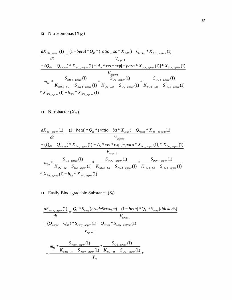
87
q Nitrosomonas (XSO)
q Nitrobacter (Xba)
q Easily Biodegradable Substance (Sf)
1
___1
1
__
)1(*)]1(*exp[**)1(*)(
)1(*)*_(**)1()1(
upper
upperSOupperSOaupperSOaboved
upper
bottomSOresusRASRupperSO
V
XXparavelAXQQ
V
XQXsoratioQbeta
dt
dX
−−+−
++−
=
)1(*)1(*
)1(
)1(*
)1(
)1(*
)1(
)1(*
)1(*)]1(*exp[**)1(*)(
)1(*)*_(**)1()1(
__
_4_4
_4
_2_2
_2
_2_2
_2
1
___1
1
__
upperbabaupperba
upperPObaPO
upperPO
upperNObaNO
upperNO
upperObaO
upperOba
upper
upperbaupperbaaupperbaaboved
upper
bottombaresusRASRupperba
XbX
SK
S
SK
S
SK
S
V
XXparavelAXQQ
V
XQXbaratioQbeta
dt
dX
−
++++
−−+−
++−
=
µ
)1(*)1(*
)1(
)1(*
)1(
)1(*
)1(
)1(*
__
_4_4
_4
_2_2
_2
_4_4
_4
upperSOSOupperSO
upperPOSOPO
upperPO
upperOSOO
upperO
upperNHSONH
upperNHSO
XbX
SK
S
SK
S
SK
S
−
++++ µ
1
__1
1
_
)1(*)1(*)(
)3(**)1()(*)1(
upper
bottomeasyresusuppereasydabove
upper
easyReasyIuppereasy
V
SQSQQ
V
thickenSQbetaecrudeSewagSQ
dt
dS
++−
+−+
=
*)1(
)1(*
)1(
)1(*
_2_2
_2
__
_
H
upperOHO
upperO
uppereasyHeasy
uppereasyH
Y
SK
S
SK
S
++−
µ

88
q Fermentation Products (SA)
q Heterotroph (XH)
)1(*)1(/)1(
)1(/)1(*
)1(
)1(*
)1(*)1(
)1(*
)1(
)1(
____
__
_2_2
_2
__4_4
_4
_4_4
_4
upperHupperHupperslowHX
upperHupperslow
upperOHO
upperOH
H
upperHupperPOHPO
upperPO
upperNHHNH
upperNH
XXSK
XS
SK
SK
Y
XSK
S
SK
S
+++
++
1
__1
1
_
)1(*)1(*)(
)3(**)1()(*)1(
upper
bottomAresusupperAdabove
upper
ARAIupperA
V
SQSQQ
VthickenSQbetaecrudeSewagSQ
dt
dS
++−
+−+
=
)1(*
)1(*)1(/)1(
)1(/)1(*
)1(
)1(*
_
___
__
__
_
upperPHAPHA
upperPAOupperPAOupperPPPP
upperPAOupperPP
upperAPAOA
upperAPHA
Xb
XXXK
XX
SK
Sq
+
++−
)1(*
)1(*)1(
)1(*
_
__4_4
_4
upperHH
upperHupperPOHPO
upperPO
Xb
XSK
S
−
+
)1(
)1(*
)1(
)1(*
)1(
)1(*
)1(*)]1(*exp[**)1(*)(
)1(*)*_(**)1()1(
_4_4
_4
_2_2
_2
__
_
1
___1
1
__
upperNHHNH
upperNH
upperOHO
upperO
uppereasyHeasy
uppereasyH
upper
upperHupperHaupperHaboved
upper
bottomHresusRASRupperH
SK
S
SK
S
SK
S
V
XXparavelAXQQ
V
XQXhratioQbeta
dt
dX
++++
−−+−
++−
=
µ

89
q Slowly Biodegradable Substance (XS)
q Ortho-phosphate-P (SPO4)
+−+
=1
_ )3(**)1()(*)1(
upper
slowRslowIupperslow
VthickenXQbetaecrudeSewagXQ
dt
dX
)]1(*
)1(*)1(*)1(*[*)1(
)1(*)1(/)1(
)1(/)1(*
)1(
)1(*
)1(*)]1(*exp[**
)1(*)1(*)(
_
___
____
__
_2_2
_2
1
__
1
__1
upperPAOPAO
upperHhupperbabauppersosoX
upperHupperHupperslowHX
upperHupperslow
upperOHO
upperOH
upper
upperslowupperslowa
upper
bottomslowresusupperslowdabove
Xb
XbXbXbf
XXXK
XX
SK
SK
V
XXparavelA
V
XQXQQ
I
+
++−+
++−
−−
+++−
1
_4_41
1
44_4
)1(*)1(*)(
)3(**)1()(*)1(
upper
bottomPOresusupperPOdabove
upper
PORPOIupperPO
V
SQSQQ
VthickenSQbetaecrudeSewagSQ
dt
dS
++−
+−+
=
)1(*)1(
)1(*
)1(
)1(* _
_4_4
_4
_2_2
_2upperPAO
upperPOPAOPO
upperPO
upperOPAOO
upperOPP X
SK
S
SK
Sq
++−

90
q Phosphorus-Accumulating Organisms (XPAO)
)1(*
)]1(*)1(*)1(*)1(*[*01.0
)1(*)1(/)1(
)1(/)1(*
)1(
)1(**
)1(*)1(
)1(*
)1(
)1(*
)1(
)1(*
)1(
)1(**004.0
)1(*)1(
)1(*
)1()1(
*)1(
)1(**
)1(*)1(
)1(*
)1()1(
*)1(
)1(**
)1(*)1(/)1(
)1(/)1(*
)1(
)1(*
)1(
)1(*
)1(
)1(**
)1(/)1(
)1(/)1(*
)1(/)1(
)1(/)1(*
_
____
___
__
__
_4
__4_4
_4
_4_4
_4
_2_2
_2
__
_
_4_4
4
2_2
2
2_2
2
_4_4
4
2_2
2
4_4
4
___
__
_44
_4
_4_4
_4
_2_2
_2
__
__
__
__
upperPPPP
upperhhupperpaopaoupperbabaupperSOSO
upperPAOuppePAOupperPPPP
upperPAOupperPP
upperAPAOA
upperAPHAPO
upperHupperPOHPO
upperPO
upperNHHNH
upperNH
upperOHO
upperO
uppereasyHeasy
uppereasyH
upperbaPObaPO
PO
ObaO
O
NObaNO
NObaPBM
upperSOPOSOPO
PO
OSOO
O
NHSONH
NHSOPBM
upperPAOupperPAOupperPHAPHA
upperPAOupperPHA
upperPOPO
upperPO
upperNHpaoNH
upperNH
upperOPAOO
upperOPAOPBM
upperPAOupperPPMAXIPP
upperPAOupperPPMAX
upperPAOupperPHAPHA
upperPAOupperPHA
Xb
XbXbXbXb
XXXK
XX
SK
Sq
XSK
S
SK
S
SK
S
SK
S
XSK
SSK
SSK
Si
XSK
SSK
SSK
Si
XXXK
XX
SK
S
SK
S
SK
Si
XXKK
XXK
XXK
XX
+
++++
+++
+
+++−
+++−
+++−
+
+++−
−+
−
+
γ
µ
µ
µ
µ
)1(*
)1(*)1(/)1(
)1(/)1(*
)1(
)1(*
)1(
)1(*
)1(
)1(*
_
___
__
_44
_4
_4_4
_4
_2_2
_2
upperPAOPAO
upperPAOupperPAOupperPHAPHA
upperPAOupperPHA
upperPOPO
upperPO
upperNHpaoNH
upperNH
upperOPAOO
upperOPAO
Xb
XXXK
XX
SK
S
SK
S
SK
S
−
+
++++ µ
1
___1
1
__
)1(*)]1(*exp[**)1(*)(
)1(*)*_(**)1()1(
upper
upperPAOupperPAOaupperPAOaboved
upper
bottomPAOresusRASRupperPAO
V
XXparavelAXQQ
V
XQXpaoratioQbeta
dt
dX
−−+−
++−
=
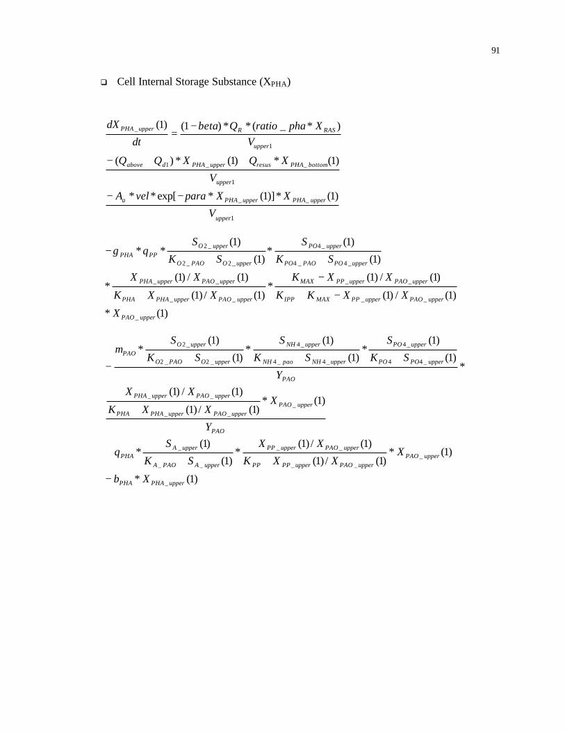
91
q Cell Internal Storage Substance (XPHA)
)1(*
)1(/)1(
)1(/)1(*
)1(/)1(
)1(/)1(*
)1(
)1(*
)1(
)1(**
_
__
__
__
__
_4_4
_4
_2_2
_2
upperPAO
upperPAOupperPPMAXIPP
upperPAOupperPPMAX
upperPAOupperPHAPHA
upperPAOupperPHA
upperPOPAOPO
upperPO
upperOPAOO
upperOPPPHA
X
XXKK
XXK
XXK
XX
SK
S
SK
Sq
−+
−
+
++− γ
1
__
1
__1
1
_
)1(*)]1(*exp[**
)1(*)1(*)(
)*_(**)1()1(
upper
upperPHAupperPHAa
upper
bottomPHAresusupperPHAdabove
upper
RASRupperPHA
V
XXparavelA
V
XQXQQ
VXpharatioQbeta
dt
dX
−−
+++−
+−
=
)1(*
)1(*)1(/)1(
)1(/)1(*
)1(
)1(*
)1(*)1(/)1(
)1(/)1(
*)1(
)1(*
)1(
)1(*
)1(
)1(*
_
___
__
__
_
___
__
_44
_4
_4_4
_4
_2_2
_2
upperPHAPHA
upperPAOupperPAOupperPPPP
upperPAOupperPP
upperAPAOA
upperAPHA
PAO
upperPAOupperPAOupperPHAPHA
upperPAOupperPHA
PAO
upperPOPO
upperPO
upperNHpaoNH
upperNH
upperOPAOO
upperOPAO
Xb
XXXK
XX
SK
Sq
Y
XXXK
XXY
SK
S
SK
S
SK
S
−
+++
+
+++−
µ

92
q Poly-P (XPP)
q Dissolved Oxygen (SO2)
)1(*)1(
)1(*
)1(
)1(*
)1(
)1(*
)1(
)1(**)
11(
)1(*)1(
)1(*
)1(
)1(*
)1(
)1(**)
14.11(
)1(*)1(
)1(*
)1(
)1(*
)1(
)1(**)
43.31(
)1(*)1(*)(
)]1([**1)1(
__4_4
_4
_4_4
_4
_2_2
_2
__
_
__4_4
_4
_2_2
_2
_2_2
_2
__4_4
_4
_2_2
_2
_4_4
_4
1
_2_21
_2_2
upperHupperPOHPO
upperPO
upperNHHNH
upperNH
upperOHO
upperO
uppereasyHeasy
uppereasyH
H
upperbaupperPObaPO
upperPO
upperNObaNO
upperNO
upperObaO
upperOba
ba
upperSOupperPOSOPO
upperPO
upperOSOO
upperO
upperNHSONH
upperNHSO
SO
upper
bottomOresusupperOdabove
upperOSupperO
XSK
S
SK
S
SK
S
SK
S
Y
XSK
S
SK
S
SK
S
Y
XSK
S
SK
S
SK
S
Y
V
SQSQQ
SCconstndt
dS
++
++−+
+
++−+
+
++−+
++−
+−=
µ
µ
µ
)1(*
)1(*)1(/)1(
)1(/)1(*
)1(
)1(**
)1(*
)1(/)1(
)1(/)1(*
)1(/)1(
)1(/)1(*
)1(
)1(*
)1(
)1(*
)1(*)]1(*exp[**)1(*
)1(*)(_***)1()1(
_
___
__
__
_4
_
__
__
__
__
_4_4
_4
_2_2
_2
1
___
1
_1_
upperPPPP
upperPAOuppePAOupperPPPP
upperPAOupperPP
upperAPAOA
upperAPHAPO
upperPAO
upperPAOupperPPMAXIPP
upperPAOupperPPMAX
PHAupperPAOupperPHA
upperPAOupperPHA
PAOPOupperPO
upperPO
PAOOupperO
upperOPP
upper
upperPPupperPPabottomPPresus
upper
upperPPdaboveRRupperPP
Xb
XXXK
XX
SK
Sq
X
XXKK
XXK
KXX
XX
KS
S
KS
Sq
V
XXparavelAXQ
V
XQQppratioXQbeta
dt
dX
−
++−
−+
−
+
+++
−−
++−−
=
γ

93
)1(*)1(/)1(
)1(/)1(*
)1(/)1(
)1(/)1(*
)1(
)1(*
)1(
)1(**
)]1(*)1(/)1(
)1(/)1(*
)1(
)1(*
)1(
)1(*
)1(
)1(*[*)
11(
___
__
__
__
_4_4
_4
_2_2
_2
___
__
_44
_4
_4_4
_4
_2_2
_2
upperPAOupperPAOupperPPMAXIPP
upperPAOupperPPMAX
PHAupperPAOupperPHA
upperPAOupperPHA
PAOPOupperPO
upperPO
PAOOupperO
upperOPPPHA
upperPAOupperPAOupperPHAPHA
upperPAOupperPHA
upperPOPO
upperPO
upperNHpaoNH
upperNH
upperOPAOO
upperOPAO
PAO
XXXKK
XXK
KXX
XX
KS
S
KS
Sq
XXXK
XX
SK
S
SK
S
SK
S
Y
−+
−
+
++−
+
+++−+
γ
µ
Table 4.4 Differential Equations for the Bottom First CSTR Element in the Aerator (all notations are given in Table 4.1 and 4.2)
q Ammonium (SNH4)
)1(*
)1(/)1(
)1(/)1(*
)1(
)1(***01.0
)1(*)1(
)1(*
)1(**03.0
)1(*)(
)1(*)3(**)1(
_
___
__
_3_3
_33
__
_
_3_3
_3
1
_4
1
_414_4
bottomH
bottomHbottomslowHX
bottomHbottomslow
bottomNOHNO
bottomNONOH
bottomHbottomeasyfe
bottomeasy
bottomNOHNO
HNOfe
bottom
bottomNHbottomresus
bottom
upperNHdNHRbottomNH
X
XSK
XS
SK
SK
XSK
S
SK
Kq
V
SQQ
V
SQthickenSQbeta
dt
dS
+++
+++
+−
++
=
η
)1(*)1(
)1(*
)1(
)1(*
)1(
)1(*
)1(
)1(***022.0
__4_4
_4
_4_4
_4
_3_3
_3
__
_3
bottomHbottomPOHPO
bottomPO
bottomNHHNH
bottomNH
bottomNOHNO
bottomNO
bottomeasyHeasy
bottomeasyNOH
XSK
S
SK
S
SK
S
SK
S
++
++− ηµ
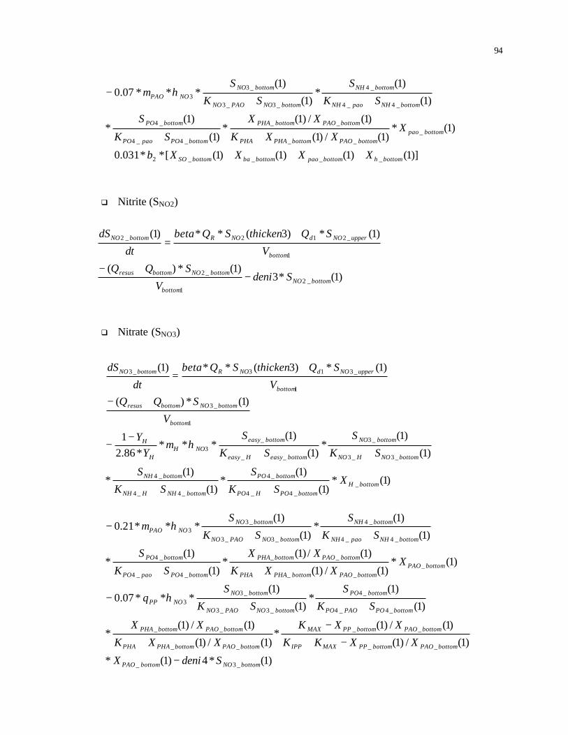
94
q Nitrite (SNO2)
q Nitrate (SNO3)
)]1()1()1()1([**031.0
)1(*)1(/)1(
)1(/)1(*
)1(
)1(*
)1(
)1(*
)1(
)1(***07.0
____2
___
__
_4_4
_4
_4_4
_4
_3_3
_33
bottomhbottompaobottombabottomSO
bottompaobottomPAObottomPHAPHA
bottomPAObottomPHA
bottomPOpaoPO
bottomPO
bottomNHpaoNH
bottomNH
bottomNOPAONO
bottomNONOPAO
XXXXb
XXXK
XX
SK
S
SK
S
SK
S
++++
++
++− ηµ
)1(*3)1(*)(
)1(*)3(**)1(
_21
_2
1
_212_2
bottomNObottom
bottomNObottomresus
bottom
upperNOdNORbottomNO
SdeniV
SQQ
V
SQthickenSQbeta
dt
dS
−+−
++
=
)1(*)1(
)1(*
)1(
)1(*
)1(
)1(*
)1(
)1(***
*86.21
)1(*)(
)1(*)3(**)1(
__4_4
_4
_4_4
_4
_3_3
_3
__
_3
1
_3
1
_313_3
bottomHbottomPOHPO
bottomPO
bottomNHHNH
bottomNH
bottomNOHNO
bottomNO
bottomeasyHeasy
bottomeasyNOH
H
H
bottom
bottomNObottomresus
bottom
upperNOdNORbottomNO
XSK
S
SK
S
SK
S
SK
S
YY
V
SQQV
SQthickenSQbeta
dt
dS
++
++−
−
+−
++
=
ηµ
)1(*4)1(*
)1(/)1(
)1(/)1(*
)1(/)1(
)1(/)1(*
)1(
)1(*
)1(
)1(***07.0
)1(*)1(/)1(
)1(/)1(*
)1(
)1(*
)1(
)1(*
)1(
)1(***21.0
_3_
__
__
__
__
_4_4
_4
_3_3
_33
___
__
_4_4
_4
_4_4
_4
_3_3
_33
bottomNObottomPAO
bottomPAObottomPPMAXIPP
bottomPAObottomPPMAX
bottomPAObottomPHAPHA
bottomPAObottomPHA
bottomPOPAOPO
bottomPO
bottomNOPAONO
bottomNONOPP
bottomPAObottomPAObottomPHAPHA
bottomPAObottomPHA
bottomPOpaoPO
bottomPO
bottomNHpaoNH
bottomNH
bottomNOPAONO
bottomNONOPAO
SdeniX
XXKK
XXK
XXK
XX
SK
S
SK
Sq
XXXK
XX
SK
S
SK
S
SK
S
−
−+
−
+
++−
++
++−
η
ηµ

95
q Nitrosomonas (XSO)
q Nitrobacter (Xba)
q Easily Biodegradable Substance (Sf)
)1(*
)1(*)]1(*exp[**)1(*)(
)1(*)_*(**)1(
_2
1
___
1
_1_
bottomSO
bottom
upperSOupperSOabottomsobottomresus
bottom
uppersodRRbottomSO
XbV
XXparavelAXQQ
V
XQsoratioXQbeta
dt
dX
−
−++−
++
=
)1(*
)1(*)]1(*exp[**)1(*)(
)1(*)_*(**)1(
_2
1
___
1
_1_
bottomba
bottom
upperbaupperbaabottombabottomresus
bottom
upperbadRRbottomba
XbV
XXparavelAXQQ
V
XQbaratioXQbeta
dt
dX
−
−++−
++
=
)1(*)1(/)1(
)1(/)1(*
)1(
)1(**
)1(*)1(
)1(
*
)1(
)1(*
)1(
)1(*
)1(
)1(**
)1(*)1(
)1(*
)1(*
)1(*)(
)1(*)3(**)1(
____
__
_3_3
_33
__4_4
_4
_4_4
_4
_3_3
_3
__
_3
__
_
_3_3
_3
1
_
1
_1_
bottomHbottomHbottomslowHX
bottomHbottomslow
bottomNOHNO
bottomNONOH
H
bottomHbottomPOHPO
bottomPO
H
bottomNHHNH
bottomNH
bottomNOHNO
bottomNO
bottomeasyHeasy
bottomeasyNOH
bottomHbottomeasyfe
bottomeasy
bottomNOHNO
HNOfe
bottom
bottomeasybottomresus
bottom
uppereasydeasyRbottomeasy
XXSK
XS
SK
SK
Y
XSK
SY
SK
S
SK
S
SK
S
XSK
S
SK
Kq
V
SQQV
SQthickenSQbeta
dt
dS
+++
+
+++−
++−
+−
++
=
η
ηµ

96
q Fermentation Product (SA)
q Heterotroph (XH)
q Slowly Biodegradable Substance (XS)
1
_
1
_1_
)1(*)(
)1(*)3(**)1(
bottom
bottomAbottomresus
bottom
upperAdARbottomA
V
SQQ
V
SQthickenSQbeta
dt
dS
+−
++
=
)]1()1()1()1([**)1(
)1(*)1(/)1(
)1(/)1(*
)1(
)1(**
)1(*)]1(*exp[**)1(*)(
)1(*)3(**)1(
____2
____
__
_3_3
_33
1
___
1
_1_
bottomPAObottomHbottombabottomsoX
bottomHbottomHbottomslowHX
bottomHbottomslow
bottomNOHNO
bottomNONOH
bottom
upperSlowupperslowabottomslowbottomresus
bottom
upperslowdslowRbottomslow
XXXXbf
XXXK
XX
SK
SK
V
XXparavelASQQV
XQthickenXQbeta
dt
dX
I+++−+
++−
−++−
++
=
η
)1(*
)1(*)1(
)1(*
)1(
)1(*
)1(
)1(*
)1(
)1(**
)1(*)]1(*exp[**)1(*)(
)1(*)_*(**)1(
_2
__4_4
_4
_4_4
_4
_3_3
_3
__
_3
1
___
1
_1_
bottomH
bottomHbottomPOHPO
bottomPO
bottomNHHNH
bottomNH
bottomNOHNO
bottomNO
bottomeasyHeasy
bottomeasyNOH
bottom
upperHupperHabottomHbottomresus
bottom
upperHdRRbottomH
Xb
XSK
S
SK
S
SK
S
SK
SV
XXparavelAXQQ
V
XQhratioXQbeta
dt
dX
−
++
+++
−++−
++
=
ηµ
)1(*)1(*)1(
)1(*
)1(*
)1(*)1(/)1(
)1(/)1(*
)1(
)1(*
___
_
_3_3
_3
___
__
__
_
bottomPHAPHAbottomHbottomeasyfe
bottomeasy
bottomNOHNO
HNOfe
bottomPAObottomPAObottomPPPP
bottomPAObottomPP
bottomApaoA
bottomAPHA
XbXSK
S
SK
Kq
XXXK
XX
SK
Sq
+++
+
++−

97
q Ortho-phosphate-P (SPO4)
)1(*)1(
)1(*
)1(
)1(*
)1(
)1(*
)1(
)1(***004.0
)1(/)1(
)1(/)1(*
)1(/)1(
)1(/)1(*
)1(*)1(
)1(*
)1(
)1(**
)1(*)1(
)1(*
)1(**01.0
)1(*)1(/)1(
)1(/)1(*
)1(
)1(**
)1(*)(
)1(*)3(**)1(
__4_4
_4
_4_4
_4
_3_3
_3
__
_3
__
__
__
__
__4_4
_4
_3_3
_33
__
_
_3_3
_3
___
__
__
_4
1
_4
1
_414_4
bottomHbottomPOHPO
bottomPO
bottomNHHNH
bottomNH
bottomNOHNO
bottomNO
bottomeasyHeasy
bottomeasyNOH
bottomPAObottomPPMAXIPP
bottomPAObottomPPMAX
bottomPAObottomPHAPHA
bottomPAObottomPHA
bottomPAObottomPOpaoPO
bottomPO
bottomNOPAONO
bottomNONOPP
bottomHbottomeasyfe
bottomeasy
bottomNOHNO
HNOfe
bottomPAObottomPAObottomPPPP
bottomPAObottomPP
bottomAPAOA
bottomAPHAPO
bottom
bottomPObottomresus
bottom
upperPOdPORbottomPO
XSK
S
SK
S
SK
S
SK
S
XXKK
XXK
XXK
XX
XSK
S
SK
Sq
XSK
S
SK
Kq
XXXK
XX
SK
Sq
V
SQQV
SQthickenSQbeta
dt
dS
++
++−
−+
−
+
++−
+++
+++
+−
++
=
ηµ
η
γ
)1(*
)]1()1()1()1([**01.0
)1(*)1(/)1(
)1(/)1(*
)1(
)1(*
)1(
)1(*
)1(
)1(***
_
____2
___
__
_4_4
_4
_4_4
_4
_3_3
_33
bottomPPPP
bottomhbottompaobottombabottomSO
bottomPAObottomPAObottomPHAPHA
bottomPAObottomPHA
bottomPOpaoPO
bottomPO
bottomNHpaoNH
bottomNH
bottomNOPAONO
bottomNONOPAOPBM
Xb
XXXXb
XXXK
XX
SK
S
SK
S
SK
Si
+
++++
++
++− ηµ

98
q Phosphorus-Accumulating Organism (XPAO)
q Cell Internal Storage Substance (XPHA)
++
=1
_1_ )1(*)_*(**)1(
bottom
upperPAOdRRbottomPAO
V
XQpaoratioXQbeta
dt
dX
)1(/)1(
)1(/)1(*
)1(/)1(
)1(/)1(*
)1(*)1(
)1(*
)1(
)1(*
)1(*)1(/)1(
)1(/)1(*
)1(
)1(*
)1(*)]1(*exp[**)1(*)(
)1(*_***)1(
__
__
__
__
__4_4
_4
_3_3
_3
___
__
__
_
1
___
1
_1_
bottomPAObottomPPMAXIPP
bottomPAObottomPPMAX
bottomPAObottomPHAPHA
bottomPAObottomPHA
bottomPAObottomPOPAOPO
bottomPO
bottomNOPAONO
bottomNOPPPHA
bottomPAObottomPAObottomPPPP
bottomPAObottomPP
bottomAPAOA
bottomAPHA
bottom
upperPHAupperPHAabottomPHAbottomresus
bottom
upperPHAdRRbottomPHA
XXKK
XXK
XXK
XX
XSK
S
SK
Sq
XXXK
XX
SK
Sq
V
XXparavelAXQQ
V
XQpharatioXQbeta
dt
dX
−+
−
+
++−
+++
−++−
++
=
γ
)1(*
)1(*)1(/)1(
)1(/)1(*
)1(
)1(*
)1(
)1(*
)1(
)1(**
)1(*)]1(*exp[**)1(*)(
_2
___
__
_4_4
_4
_4_4
_4
_3_3
_33
1
___
bottomPAO
bottompaobottomPAObottomPHAPHA
bottomPAObottomPHA
bottomPOpaoPO
bottomPO
bottomNHpaoNH
bottomNH
bottomNOPAONO
bottomNONOPAO
bottom
upperPAOupperPAOabottomPAObottomresus
Xb
XXXK
XX
SK
S
SK
S
SK
S
V
XXparavelAXQQ
−
++
+++
−++−
ηµ

99
q Poly-P (XPP)
q Dissolved Oxygen (SO2)
1
_2_2_21_2 )1(*)1(*)1(*)1(
bottom
bottomObottombottomOresusupperOdbottomO
V
SQSQSQ
dt
dS −−=
Those equations in Table 6.3 and 6.4 include not only features of characterization
of solids and nutrient transport in the aeration tank, but also the two-step nitrification
process from ammonium to nitrite and then nitrate, and simultaneous nitrification and
denitrification in the upper CSTRs. Nitrogen losses from aerated facilities have been
observed frequently (Applegate et al., 1980; Drews and Greef, 1973; Rittmann and
Langeland, 1985; van Huyssteen et al., 1990; van Munch et al., 1996; Bertanza,1997). As
quoted in Chapter 2, O’Neill et al. (1995) reported that simultaneous nitrification and
denitrification in the outer lane of the Orbal process took place in the presence of a DO
concentration of 1.5 mg/L. The biochemistry of ortho-phosphate-P removal in the current
model is based on that is proposed in ASM2.
)1(*)1(*
)1(/)1(
)1(/)1(*
)1(/)1(
)1(/)1(*
)1(
)1(*
)1(
)1(**)1(*
)1(/)1(
)1(/)1(*
)1(
)1(**
)1(*)]1(*exp[**)1(*)(
)1(**_**)1(
__
__
__
__
__
_4_4
_4
_3_3
_33_
__
__
__
_4
1
___
1
_1_
bottomPPPPbottoomPAO
bottomPAObottomPPMAXIPP
bottomPAObottomPPMAX
PHAbottomPAObottomPHA
bottomPAObottomPHA
bottomPOpaoPO
bottomPO
bottomNOPAONO
bottomNONOPPbottomPAO
PPbottomPAObottomPP
bottomPAObottomPP
bottomAPAOA
bottomAPHAPO
bottom
upperPPupperPPabottomPPbottomresus
bottom
upperPPdRASRbottomPP
XbX
XXKK
XXK
KXX
XX
SK
S
SK
SqX
KXX
XX
SK
Sq
V
XXparavelAXQQV
XQXppratioQbeta
dt
dX
−
−+
−
+
+++
++−
−++−
++
=
η
γ

100
4.5 SECONDARY CLARIFIER MODEL STRUCTURE
In the Athens Wastewater Treatment Facility case study, only one secondary
clarifier was monitored for its dynamic behavior. Therefore, it is assumed that the
aeration tank effluent is equally distributed among the three secondary clarifiers, and that
equal amounts of wastage sludge are drawn from each individual clarifier. In the
secondary clarifier, particulate transport is characterized based on the classical flux
theory (Dick & Young, 1972), with the solutes simply being routed through each
individual CSTR in the thickening zone, compaction zone, and clarification zone,
assuming that no biochemical reactions take place there. As drawn in Figure 4.1, the
secondary clarifier is represented by three conceptual zones, i.e., clarification, thickening,
and compaction zones. The descriptions for each of these sub-models are given below.
4.5.1 Clarification Sub-Model
The volume of the clarification zone varies due to the time-varying nature of the
sludge blanket level in the thickening zone, and is equal to the volume of the secondary
clarifier above the sludge blanket. The mixing characteristics of the clarification zone are
approximated by 4 identical CSTR elements in the vertical direction of variable volumes
by calibration.
4.5.1.1 Characterization of Solute Matter in the Clarification Zone
Seven soluble state variables are quantified in the clarification sub-model.
Effluent from the aeration tank is the input to three secondary clarifiers. Their
compositions in the influent to the clarification zone are assumed to be equal to their
compositions in the effluent from the aerator. They are routed in a simple manner through
the CSTR elements as follows (Table 4.5).
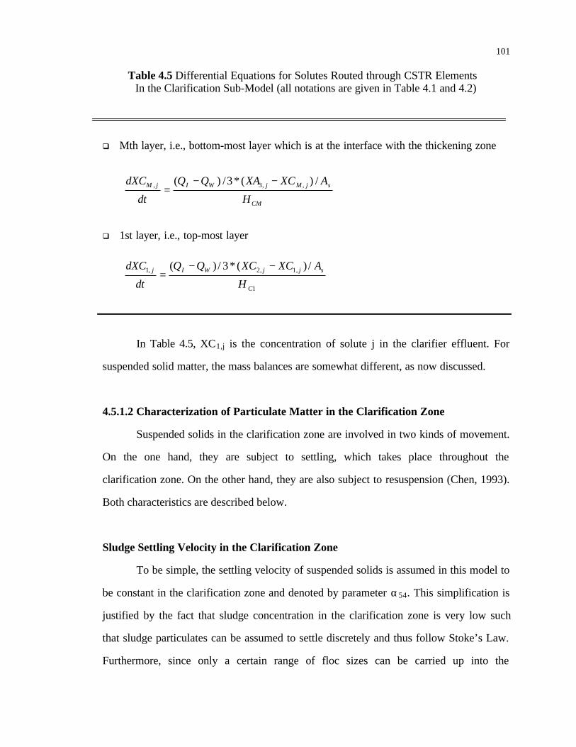
101
Table 4.5 Differential Equations for Solutes Routed through CSTR Elements In the Clarification Sub-Model (all notations are given in Table 4.1 and 4.2)
q Mth layer, i.e., bottom-most layer which is at the interface with the thickening zone
q 1st layer, i.e., top-most layer
In Table 4.5, XC1,j is the concentration of solute j in the clarifier effluent. For
suspended solid matter, the mass balances are somewhat different, as now discussed.
4.5.1.2 Characterization of Particulate Matter in the Clarification Zone
Suspended solids in the clarification zone are involved in two kinds of movement.
On the one hand, they are subject to settling, which takes place throughout the
clarification zone. On the other hand, they are also subject to resuspension (Chen, 1993).
Both characteristics are described below.
Sludge Settling Velocity in the Clarification Zone
To be simple, the settling velocity of suspended solids is assumed in this model to
be constant in the clarification zone and denoted by parameter α54. This simplification is
justified by the fact that sludge concentration in the clarification zone is very low such
that sludge particulates can be assumed to settle discretely and thus follow Stoke’s Law.
Furthermore, since only a certain range of floc sizes can be carried up into the
CM
sjMjWIjM
H
AXCXAQQ
dt
dXC /)(*3/)( ,,3, −−=
1
,1,2,1 /)(*3/)(
C
sjjWIj
H
AXCXCQQ
dt
dXC −−=

102
clarification zone and then settle (Mueller et al., 1967; Magara et al., 1976; Otterpohl and
Freund, 1992), it is reasonable to assume that the distributions of floc density and
diameter for settleable suspended solids in the clarification zone do not show significant
variations. As a result, it is acceptable to assume that their average settling velocity is
largely invariant with time.
Sludge Resuspension in the Clarification Zone
The feed point for the secondary clarifier is below the surface of the unit. Upon
entering the secondary clarifier, the solids stream is assumed to behave as a submerged
waterfall passing entirely into the thickening zone. Therefore, any suspended solids
subsequently found in the clarification zone are there as a result of resuspension from the
thickening zone. Resuspension occurring at the interface layer between the clarification
zone and the thickening zone is characterized by a mass flux in the model below denoted
by Qt t. The resuspension flow can be related to a number of factors, among which
hydraulic shocks are the most important (Zhou and McCorquodale, 1992; Chen, 1993).
The resuspension flow is quantified as follows (Chen, 1993):
where,
α45−Minimum suspended solids flux. In other words, there is always some upward
movement of particles into the clarification zone ;
α46−Hydraulic effect factor;
XMLSS−MLSS from inner channel of the aeration tank.
These two components constitute a form of Pflanz empirical expression for
relating the transfer flux into the clarifier to both the flow rate and suspended solids
concentration of the influent to the secondary clarifier (Pflanz, 1969; Takacs, 1986).
MLSSintt XQQ **4645 αα +=
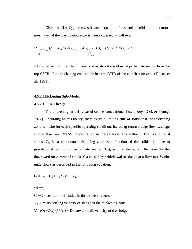
103
Given the flux Qt t, the mass balance equation of suspended solids in the bottom-
most layer of the clarification zone is then expressed as follows:
where the last term on the numerator describes the upflow of particulate matter from the
top CSTR of the thickening zone to the bottom CSTR of the clarification zone (Takacs et
al., 1991).
4.5.2 Thickening Sub-Model
4.5.2.1 Flux Theory
The thickening model is based on the conventional flux theory (Dick & Young,
1972). According to this theory, there exists a limiting flux of solids that the thickening
zone can take for each specific operating condition, including return sludge flow, wastage
sludge flow, and MLSS concentration in the aeration tank effluent. The total flux of
solids, Gt, in a continuous thickening zone is a function of the solids flux due to
gravitational settling of particulate matter (Gg), and of the solids flux due to the
downward movement of solids (Gu) caused by withdrawal of sludge at a flow rate Vu (the
underflow), as described in the following equation:
Gt = Gg + Gu = Ci * (Vs + Vu)
where,
Ci −Concentration of sludge in the thickening zone;
Vs−Gravity settling velocity of sludge in the thickening zone;
Vu=(QR+QW)/(3*AS) − Downward bulk velocity of the sludge.
CM
sMWIMMttM
H
AXCQQXCXCQ
dt
dXC /*3/)()(* 1,1,1,1541, −−−+= −α

104
Any applied flux exceeding the limiting flux will result in a continual increase of
the sludge blanket as long as the applied flux is higher than the limiting flux. The sludge
blanket concentration will then be equal to the limiting concentration corresponding to
the limiting flux associated with the given operating condition (Dick & Young, 1972).
4.5.2.2 Representative Equations
The thickening zone is represented by 2 CSTR elements with variable volume by
calibration, where variation is due to the increase or decrease of the sludge blanket
height. When there is no blanket, the compression layer is fed directly by the aeration
tank effluent. The concentration of suspended solids in the upper-most layer of the
thickening zone is never allowed to exceed the limiting concentration defined by the flux
theory for the given operating conditions. But once at its limiting concentration, the
blanket volume is allowed to expand with overloading or to contract with underloading.
The compaction zone, on the other hand, comprises just one CSTR element with fixed
volume by calibration as shown in Figure 5.1.
Eight state variables are simulated in the thickening zone model: seven for the
solute state variables and one for the particulate state variables. The seven solute state
variables are routed through the thickening zone and the compaction zone as
conservative, non-reacting substances. The feed point for the secondary clarifier is
located near the surface of the unit, and the solids stream is assumed to behave as a
submerged waterfall entering the sludge blanket at height HSBM directly.
For the uppermost layer of the thickening zone, the suspended solids
concentration is described as:
SBM
uisjittjsinRIji
H
VVXBQXCAXQQ
dt
dXB )(*1*/*]3/)[(1 ,,,154, +−−++=
α

105
where,
Xin −Suspended solids concentration from the aerator to the secondary clarifier;
XC1,j−Suspended solids concentration at the bottom-most CSTR of the clarification zone.
After each iteration of the calculation, the resulting concentration of the blanket
will be checked against the flux theory. If a violation has occurred, such as exceeding the
limiting concentration, the concentration of the blanket will be reset to the limiting value
with the flux imbalance being provided for by an increase in the blanket height.
For the layer beneath the uppermost layer of the thickening zone:
For the compaction zone:
The volume of the compaction zone is invariant. The settling velocity of the
suspended solids in the thickening zone is described by an exponential function as
follows (Dick and Young, 1972):
Vs=max_vel*exp(-para*X)
where,
max_vel and para −Constants;
X−Suspended solids concentration in each individual CSTR.
SBi
uisjiuisjiji
H
VVXBVVXB
dt
dXB )(*1)(*11 1,,1,,,1 +−+= −−−
CZ
uRASusjRAS
H
VXBVVXB
dtdXB *2)(*12 1,,1 −+
=

106
4.6 DISCUSSIONS
4.6.1 Assumptions and Restrictions Associated With the Model
As with every model, the proposed model is certainly a compromise. Inevitably it
has some assumptions and restrictions, which are summarized as follows:
q During the simulation, it is assumed that there is no evidence of any abnormal
behavior, such as sludge bulking taking place;
q The system operated at a constant pH level;
q The concentration of suspended solids is completely uniform within any vertical layer
within the thickening zone;
q The mass flux into the top CSTR of the thickening zone cannot exceed the mass flux
that element is capable of taking, nor can it exceed the mass flux which the element
immediately below it is capable of taking;
q The gravitational settling velocity of solids in the thickening zone and the compaction
zone is a function of the suspended solids concentration;
q No significant biological reactions take place in the secondary clarifier.
4.6.2 Implementation of the Model
A computer program written in Matlab was developed for use on a PC. The
simulation results from the program were then analyzed within the environment of
Matlab in terms of checking the model results against the real data.
4.7 CONCLUSIONS
A dynamic multiple species model has been developed and presented in this
Chapter for simulating nutrient removal processes in the activated sludge process. Its
major innovations compared to ASM2 are:
q Characterization of solute and particulate transport in the activated sludge process;
107
q Differentiation of functions of Nitrosomonas and Nitrobacter in the nitrification
process;
q Characterization of simultaneous nitrification and denitrification in the aerated
environment.
The proposed model will be used to improve understanding of activated sludge
process performance under dynamic conditions. A detailed examination of the model,
i.e., calibration by trial and error, validation and sensitivity analysis, follows in Chapter 5.

108
CHAPTER 5
MODEL CALIBRATION, VALIDATION, AND SENSITIVITY ANALYSIS
5.1 INTRODUCTION
A comprehensive dynamic model has been developed in the preceding chapter.
Now it is time to assess the validity of the model’s structure, in particular in respect of its
novel features. The calibration method adopted hereby is trial-and-error. However, in
identifying such a complicated model with so many parameters the harsh reality is that it
is hard to retrieve a uniquely best set of parameters when checked against real world data.
In section 5.2 calibration results are presented, and possible reasons for mismatches
between model results and data are discussed. Thereafter, another set of data is used for
model validation in section 5.3. Sensitivity analysis is finally carried out at the end of this
Chapter in section 5.4.
5.2 MODEL CALIBRATION RESULTS AND DISCUSSIONS
The field data used for this calibration exercise were part of the data retrieved
from the comprehensive sampling campaign from the Athens Wastewater Treatment
Facility No.2 case study illustrated in Chapter 3. It is some 19 days long, from March 12,
1998 to March 31, 1998.
Shown below in Figure 5.1 is the influent flow data for the calibration period,
averaging about 4 MGD. On the 6th day there was a moderate rain event. Unfortunately,
control actions taken by the plant during the event, such as step-feed or step-sludge, were
not recorded. Figure 5.2 plots out the return sludge rate during this 19-day period. These
data were recorded roughly on a daily basis (missing for some days), and it is therefore
assumed in the model that return sludge rate remains constant over a 24h period (straight

109
line in Figure 5.2).
Figure 5.1 Influent Flow for Model Calibration
Figure 5.2 Return Sludge Flow for Model Calibration
The same applies to sludge wastage rate. Sludge processing personnel in the treatment
plant worked only 4 days a week; sludge wastage was stopped during their off days.
0 2 4 6 8 10 12 14 16 18 2
2.5
3
3.5
4
4.5
5
5.5
6
6.5
7
Time (Days)
Influ
ent F
low
(M
GD
)
0 2 4 6 8 10 12 14 16 18 1.5
2
2.5
3
Time(Days)
Com
bine
d R
etur
n S
ludg
e F
low
(MG
D)

110
Sludge wastage rate was never above 0.22 MGD due to the wastage capacity. DO
concentration in the outer channel of the aeration tank was measured by treatment plant
personnel on a daily basis, while those in the middle and inner channels were
continuously measured by the out-board DO probes of EPCL (Table 3.1). It is apparent
that DO concentration in the middle channel was consistently lower relative to those in
the other two channels. The average temperature of the sewage for the 19 days was
around 16°C. However, temperature for the last four days or so (day 14 onwards) was
about 5°C higher. PH value of the sewage stayed relatively stable at about 6.5. As cited in
Chapter 2, Wild et al. (1971) found that nitrification rate decreases below pH of 8.0 until
it is completely inhibited at pH below 5.
5.2.1 Nitrification and Denitrification
The calibration exercise started with nitrification, the reason being that this is
generally believed to be the most well defined process, and thus should be a relatively
“simple” process to identify. In order to illustrate how model results were improved by
progressively changing model structures, ammonium concentration in the outer channel
of the aeration tank is therefore selected as the focus of discussion in this section. The
outer channel is closer to the feeding points of crude sewage and return sludge compared
to middle and inner channels, and better simulation results are expected there. It is also
believed that description of how fitting for ammonium concentration in the outer channel
was achieved, step by step, should be able to give a good account of how the 2-layer
model come to be proposed.
At the beginning of the simulation exercise, nitrification was simulated as a one-
step process, from ammonium directly to nitrate, based on the configuration in ASM2
(Henze et al., 1995a). Under this configuration, nitrifiers are treated as one entity
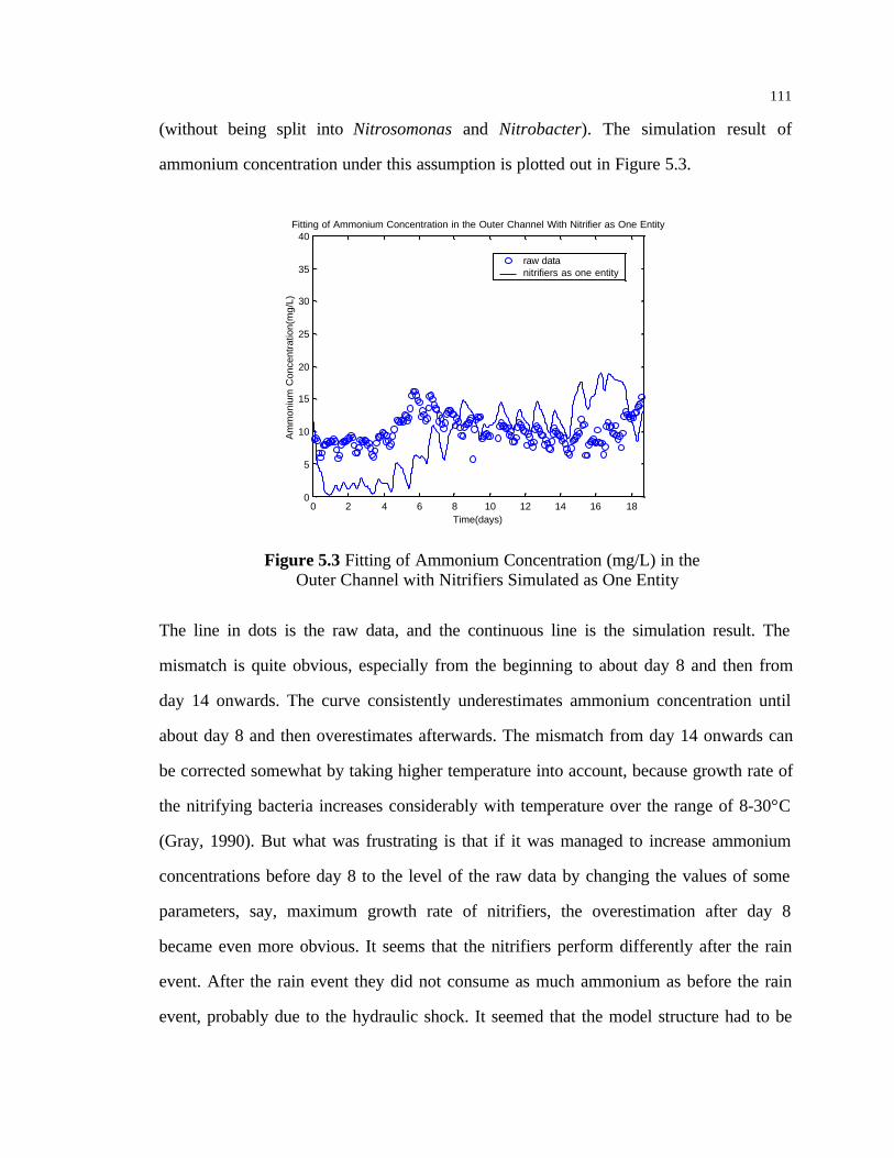
111
(without being split into Nitrosomonas and Nitrobacter). The simulation result of
ammonium concentration under this assumption is plotted out in Figure 5.3.
Figure 5.3 Fitting of Ammonium Concentration (mg/L) in the Outer Channel with Nitrifiers Simulated as One Entity
The line in dots is the raw data, and the continuous line is the simulation result. The
mismatch is quite obvious, especially from the beginning to about day 8 and then from
day 14 onwards. The curve consistently underestimates ammonium concentration until
about day 8 and then overestimates afterwards. The mismatch from day 14 onwards can
be corrected somewhat by taking higher temperature into account, because growth rate of
the nitrifying bacteria increases considerably with temperature over the range of 8-30°C
(Gray, 1990). But what was frustrating is that if it was managed to increase ammonium
concentrations before day 8 to the level of the raw data by changing the values of some
parameters, say, maximum growth rate of nitrifiers, the overestimation after day 8
became even more obvious. It seems that the nitrifiers perform differently after the rain
event. After the rain event they did not consume as much ammonium as before the rain
event, probably due to the hydraulic shock. It seemed that the model structure had to be
0 2 4 6 8 10 12 14 16 180
5
10
15
20
25
30
35
40
Time(days)
Am
mon
ium
Con
cent
ratio
n(m
g/L)
Fitting of Ammonium Concentration in the Outer Channel With Nitrifier as One Entity
raw data nitrifiers as one entity

112
adjusted somehow to relieve this predicament. It was then realized that the mismatch up
to day 8 might be corrected by associating only Nitrosomonas with ammonium removal
rather than the combination of Nitrosomonas and Nitrobacter. The reason is that even
though both nitrifiers play important roles in the nitrification process, they in fact oxidize
different substrates, i.e., Nitrosomonas oxidizes ammonium to nitrite, while Nitrobacter
subsequently oxidizes the intermediate products to nitrate, and therefore they cannot be
simply combined as one entity.
Efforts were then made to simulate nitrification as a two-step process instead of a
simple one-step process. Essentially, nitrifiers, previously assumed as an entity, were
split up into two entities, i.e., Nitrosomonas and Nitrobacter. Therefore one more state
variable, nitrite, is introduced into the model as an intermediate product. The
corresponding model result is shown in Figure 5.4.
Figure 5.4 Fitting of Ammonium Concentration (mg/L) in the Outer Channel with Nitrifiers Simulated as Two Entities
Clearly, the new model structure does a better job in matching the data before day
8 compared to Figure 5.3, even though not equally well after day 8. Undeniably, this has
been a significant improvement. Looking closer at the mismatch after day 8 in Figure 5.4,
0 2 4 6 8 10 12 14 16 180
5
10
15
20
25
30
35
40
Time(days)
Am
mon
ium
Con
cent
ratio
n(m
g/L)
Fitting of Ammonium Concentration in the Outer Channel With Nitrifiers as Two Entities
raw data nitrifiers as two entities
Rain Event
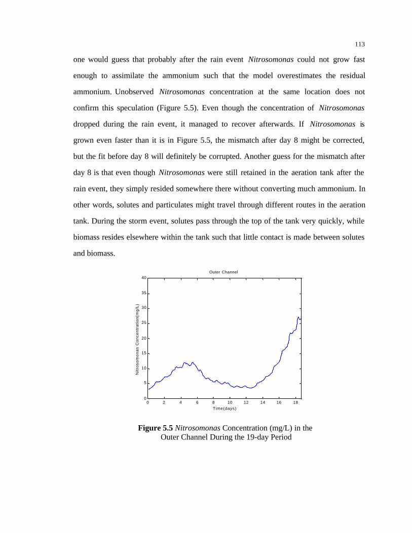
113
one would guess that probably after the rain event Nitrosomonas could not grow fast
enough to assimilate the ammonium such that the model overestimates the residual
ammonium. Unobserved Nitrosomonas concentration at the same location does not
confirm this speculation (Figure 5.5). Even though the concentration of Nitrosomonas
dropped during the rain event, it managed to recover afterwards. If Nitrosomonas is
grown even faster than it is in Figure 5.5, the mismatch after day 8 might be corrected,
but the fit before day 8 will definitely be corrupted. Another guess for the mismatch after
day 8 is that even though Nitrosomonas were still retained in the aeration tank after the
rain event, they simply resided somewhere there without converting much ammonium. In
other words, solutes and particulates might travel through different routes in the aeration
tank. During the storm event, solutes pass through the top of the tank very quickly, while
biomass resides elsewhere within the tank such that little contact is made between solutes
and biomass.
0 2 4 6 8 10 12 14 16 180
5
10
15
20
25
30
35
40
Time(days)
Nit
roso
mo
na
s C
on
cen
tra
tio
n(m
g/L
)
Outer Channel
Figure 5.5 Nitrosomonas Concentration (mg/L) in the Outer Channel During the 19-day Period

114
It appears that a 1-layer tanks-in-series model might be an oversimplification of
the reality, and the model structure needs to be further adjusted in order to improve the
model results. Attention was then directed to characterization of mixed liquor suspended
solids (MLSS) transport in the aeration tank. At this point a two-layer model was built up
with 3 CSTRs in series in both the top and bottom layers. In other words, each channel in
the aeration tank is represented by a CSTR on the top of another one at the bottom.
Volume of CSTR on the top layer represents the effective mixing volume. As a result of
this new 2-layer configuration, exchange flows (upward and downward flows) between
CSTRs on the top and the ones immediately below, and free settling of suspended solids
from top CSTRs to bottom CSTRs, need to be accounted for. The upward flow is
considered a linear function of (QR+QW)^c based on previous investigations on
suspended solids (Simons et al., 1992), where QR and QW are return sludge rate and
wastage flow rate, and c is a constant. Downward movement flows can therefore be
calculated based on mass balances around each individual CSTR on the bottom layer.
Instinctively, flow through the top CSTRs (effective mixing volume) should be much
higher than that through the bottom CSTRs (ineffective mixing volume), and the
combination of which should amount to the flow leaving the aeration tank, i.e., crude
sewage flow plus return sludge flow. Another assumption made was that due to the high
density nature of return sludge, it may well be that a small part of the return sludge settles
immediately to the bottom CSTR upon entering the aeration tank, which was backed up
by the simulation results (Section 5.5.2.1). After exhaustive “trial-and-error” model
calibration, it turns out that the free settling velocity of suspended solids from top CSTRs
to bottom CSTRs, denoted as ‘vel’ in Table 4.2, is zero, which implies that mixing in the
effective mixing zone is so good that no free settling of suspended solids occurs (Section
5.5.2.4). Figure 5.6 below shows fitting of MLSS in the inner channel of the aeration tank

115
against real data based on the 2-layer configuration. Generally speaking, the result is very
good except obvious mismatches between day 6 and 7 and around day 11.
Figure 5.6 Fitting of MLSS in the Inner Channel During the 19-day Period
Figure 5.7 MLSS in the Upper and Bottom Middle Channel
0 2 4 6 8 10 12 14 16 18 2000
2500
3000
3500
4000
4500
5000
Time(Days)
MLS
S C
once
ntra
tion(
mg/
L)
data model
0 2 4 6 8 10 12 14 16 18 2000
2500
3000
3500
4000
4500
5000
Time(Days)
MLS
S C
once
ntra
tion
(mg/
L)
MLSS in top Middle CSTR MLSS in bottom middle CSTR

116
Intuitively, MLSS should be denser in the bottom CSTRs than in the relevant top
CSTRs, and this is confirmed by the model results as well. For example, MLSS
concentration in the upper middle CSTR is higher than that in bottom middle CSTR, as
seen in Figure 5.7.
Based on this 2-layer structure, solute transport was characterized. Figure 5.8
shows the new model results in comparison with those shown in Figure 5.3 and Figure
5.4. Improvements are fairly evident. The model tracks the data reasonably well until
shortly after day 7. From day 10 to day 14 the model underestimates observed conditions.
After that the model overestimates them. One explanation is that some parameters
considered constant are in reality variable, such as effective mixing volumes due to
shifting and on and off controls of the aerators. Clearly the 2-layer model further
improves the model results after day 8 without degrading the fitting before day 8. The
step-by-step process described so far embodies a significant success in reaching a good
model structure to properly describe the nitrification dynamics in the aeration tank.
Figure 5.8 Comparison of Ammonium Concentration in the Outer Channel with Different Model Structures
0 2 4 6 8 10 12 14 16 18 0
5
10
15
20
25
30
Time(Days)
Am
mon
ium
Con
cent
ratio
n(m
g/L)
raw data nitrifiers as one entity nitrifiers as two entities new model structure

117
Comparison of model results for ammonium concentration in the inner channel
with different model structures is shown in Figure 5.9. These results are quite
encouraging as well.
Figure 5.9 Comparison of Ammonium Concentration in the Inner Channel with Different Model Structures
Fittings of nitrite and nitrate concentrations in the middle channel and secondary
clarifier effluent are shown in Figure 5.10.
0 2 4 6 8 10 12 14 16 18 0
5
10
15
20
25
Time(Days)
Am
mon
ium
Con
cent
ratio
n (m
g/L)
raw data nitrifiers as one entity nitrifiers as Nitrosomonas and Nitrobacter 2-layer model

118
Figure 5.10 Fittings of Nitrite and Nitrate Concentrations in the Middle channel of the Aeration Tank and in the Secondary Clarifier Effluent
As seen in the upper two figures in Figure 5.10, nitrite data stays at a fairly low
level and the model results largely catch the level. However, in the bottom two figures
the model overestimates nitrate in the middle channel after about day 8. In order to
correct this mismatch, different denitrification mechanisms of nitrate were tried including
introducing the actions of heterotrophic bacteria capable of denitrification in the upper
CSTRs other than in the bottom CSTRs, because according to Meiberg (1980)
denitrification can occur in the presence of oxygen. But unfortunately the mismatch
became more evident with this effort. So the results in Figure 5.10 are about the best
achievable at present. Literature show that denitrification is not only affected by oxygen
and nitrate concentrations, intermediate product concentrations, such as NO and N2O,
0 5 10 150
0.1
0.2
0.3
0.4
0.5
Time(days)
Nitr
ite C
once
ntra
tion(
mg/
L)
Nitrite Concentration In The Middle Channel
data model
0 5 10 150
0.1
0.2
0.3
0.4
0.5
Time(days)
Nitr
ite C
once
ntra
tion(
mg/
L)
Nitrite Concentration In The Clarifier Effluent
data model
0 5 10 150
1
2
3
4
5
Time(days)
Nitr
ate
Con
cent
ratio
n(m
g/L)
Nitrate Concentration In The Middle Channel
data model
0 5 10 150
1
2
3
4
5
Time(days)
Nitr
ate
Con
cent
ratio
n(m
g/L)
Nitrate Concentration In The Clarifier Effluent
data model

119
have impacts on denitrification performance as well (Skrinde and Bhagat, 1982; Snyder
et al., 1987), which are not incorporated in the model.
0 2 4 6 8 10 12 14 16 1830
35
40
45
50
55
60
Time(days)
Nit
roso
mo
na
s C
on
cen
tra
tio
n(m
g/L
)
Middle Channel
upper middle CSTR bottom middle CSTR
(a) Nitrosomonas Concentration in the upper and lower CSTRs of the middle channel
0 2 4 6 8 10 12 14 16 1845
50
55
60
65
70
75
80
85
90
95
100
Time(days)
Nitr
obac
ter
Con
cent
ratio
n(m
g/L)
Middle Channel
upper middle CSTR bottom middle CSTR
(b) Nitrobacter Concentration in the upper and lower CSTRs of the middle channel
Figure 5.11 Nitrifiers Profiles in the Upper and Lower CSTRs of the Middle Channel
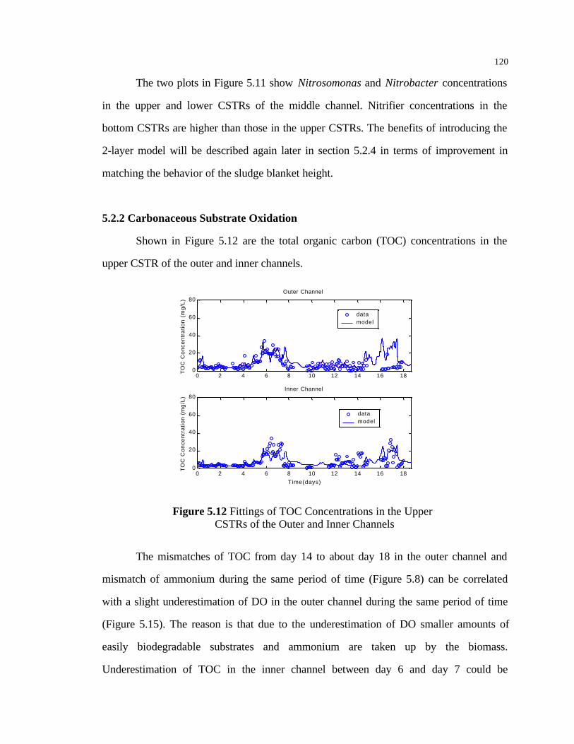
120
The two plots in Figure 5.11 show Nitrosomonas and Nitrobacter concentrations
in the upper and lower CSTRs of the middle channel. Nitrifier concentrations in the
bottom CSTRs are higher than those in the upper CSTRs. The benefits of introducing the
2-layer model will be described again later in section 5.2.4 in terms of improvement in
matching the behavior of the sludge blanket height.
5.2.2 Carbonaceous Substrate Oxidation
Shown in Figure 5.12 are the total organic carbon (TOC) concentrations in the
upper CSTR of the outer and inner channels.
0 2 4 6 8 10 12 14 16 180
20
40
60
80
TO
C C
once
ntra
tion
(mg/
L)
Outer Channel
data model
0 2 4 6 8 10 12 14 16 180
20
40
60
80
Time(days)
TO
C C
on
cen
tra
tio
n (
mg
/L)
Inner Channel
data model
Figure 5.12 Fittings of TOC Concentrations in the Upper CSTRs of the Outer and Inner Channels
The mismatches of TOC from day 14 to about day 18 in the outer channel and
mismatch of ammonium during the same period of time (Figure 5.8) can be correlated
with a slight underestimation of DO in the outer channel during the same period of time
(Figure 5.15). The reason is that due to the underestimation of DO smaller amounts of
easily biodegradable substrates and ammonium are taken up by the biomass.
Underestimation of TOC in the inner channel between day 6 and day 7 could be
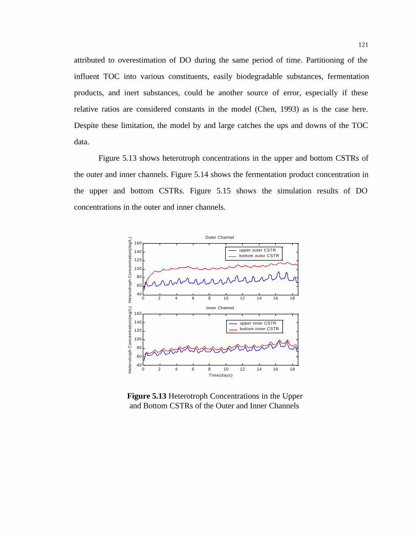
121
attributed to overestimation of DO during the same period of time. Partitioning of the
influent TOC into various constituents, easily biodegradable substances, fermentation
products, and inert substances, could be another source of error, especially if these
relative ratios are considered constants in the model (Chen, 1993) as is the case here.
Despite these limitation, the model by and large catches the ups and downs of the TOC
data.
Figure 5.13 shows heterotroph concentrations in the upper and bottom CSTRs of
the outer and inner channels. Figure 5.14 shows the fermentation product concentration in
the upper and bottom CSTRs. Figure 5.15 shows the simulation results of DO
concentrations in the outer and inner channels.
0 2 4 6 8 10 12 14 16 1840
60
80
100
120
140
160
Het
erot
roph
Con
cent
ratio
n(m
g/L) Outer Channel
upper outer CSTR bottom outer CSTR
0 2 4 6 8 10 12 14 16 1840
60
80
100
120
140
160
He
tero
tro
ph
Co
nce
ntr
atio
n(m
g/L
) Inner Channel
Time(days)
upper inner CSTR bottom inner CSTR
Figure 5.13 Heterotroph Concentrations in the Upper and Bottom CSTRs of the Outer and Inner Channels

122
Figure 5.14 Fermentation Product Concentration in the Upper and Bottom CSTRs of the Outer and Inner Channels
0 2 4 6 8 10 12 14 16 1 80
1
2
3
4
Oxy
ge
n C
on
cen
tra
tion
(mg
/L) Outer Channel
data model
0 2 4 6 8 10 12 14 16 1 80
1
2
3
4
Time(days)
Oxy
ge
n C
on
cen
tra
tio
n(m
g/L
) Inner Channel
data model
Figure 5.15 Fittings of DO Concentrations in the Outer and Inner Channel
0 2 4 6 8 10 12 14 16 18 0
10
20
30
40
Fer
men
tatio
n P
rodu
ct(m
g/L) Outer Channel
upper CSTR bottom CSTR
0 2 4 6 8 10 12 14 16 18 0
10
20
30
40
Time(Days)
Fer
men
tatio
n P
rodu
ct(m
g/L)
Inner Channel
upper CSTR bottom CSTR

123
As seen in Figure 5.15, the model consistently overestimates DO in the outer
channel from day 4 to about day 14, while it underestimates DO in the inner channel
from about day 9 until about day 15. The possible reasons for the mismatches are as
follows. Firstly, an incoming dissolved oxygen concentration of zero is assumed in the
model, which is not the case in reality (Bocken et al., 1989), especially during higher
crude sewage flows. Secondly, the oxygen transfer is not only a function of the number
of active aerators, but also several other variables including temperature, wastewater
characteristics (Casey and Karmo, 1974), and turbulence (Horan, 1989). Since there were
no DO concentration measurements for the last four days, it is assumed that DO
concentrations stay constant for the last four days, which might have contributed to the
mismatch from day 14 onwards for DO in the outer channel.
5.2.3 Phosphorus
Biological phosphorus removal is a new but quite complex process. Introduction
of a very detailed mechanistic model for the processes responsible for biological
phosphorus removal is, however, premature. Despite extensive research efforts, the
behavior and physiology of PAOs in the biological phosphate removal processes have not
yet been fully understood, as discussed in Chapter 2. The IAWQ Task Group
acknowledged the simplicity in the current model, and realized that it is the base for
further development (Henze et al., 1999).
Shown in Figure 5.16 are the simulation results of phosphorus concentrations in
the middle channel and secondary clarifier effluent, which is admittedly poor. There is an
obvious surge of phosphorus concentration in data from day 4 to day 8, which is missed
by the model. It correlates with the small surge from the rain event and very low DO in
the inner channel as seen in Figure 5.15. During the calibration process, if the surge is
better simulated, results for the rest part became much worse than what is shown in

124
Figure 5.16. Figure 5.17 shows the phosphorus-accumulating bacteria concentration in
the upper and bottom CSTR of the middle channel.
0 2 4 6 8 10 12 14 16 180
5
10
15
20
Ort
ho
-P C
on
cen
tra
tio
n(m
g/L
)
Middle Channel
data model
0 2 4 6 8 10 12 14 16 180
5
10
15
20
Time(days)
Ort
ho
-P C
on
cen
tra
tio
n(m
g/L
)
Clarifier Effluent
data model
Figure 5.16 Fittings of Ortho-phosphate-P Concentration in the Middle Channel and the Secondary Clarifier
0 2 4 6 8 10 12 14 16 18140
150
160
170
180
190
200
210
220
230
240
Time(days)
PA
O C
on
cen
tra
tio
n(m
g/L
)
Middle Channel
upper middle CSTR bottom middle CSTR
Figure 5.17 Phosphorus-Accumulating Bacteria in the Upper and Bottom CSTRs of the Middle Channel

125
According to plant operation records, no step sludge/feeding control actions were
taken around rain event on day 6, which is suspicious. But the surge in data suggests that
large amount of phosphorus might have been released due to low DO concentration
caused by under-aerated sludge. In order to interpret the data, various control alternatives
were experimented, albeit speculative. One alternative, feeding all the influent into the
inner channel while leaving the sludge in the outer channel, achieves better result in
simulating the surge (Figure 5.18). Unfortunately, by doing so simulation results for other
monitored variables, such as TOC, are seriously deteriorated.
0 2 4 6 8 10 12 14 16 180
5
10
15
Ort
ho-p
hosp
hate
-P C
once
ntra
tion(
mg/
L) Middle Channel
data model
0 2 4 6 8 10 12 14 16 180
5
10
15
Time(days)Ort
ho
-ph
osp
ha
te-P
Co
nce
ntr
ati
on
(mg
/L)
Secondary Clarifer Effluent
data model
Figure 5.18 Ortho-Phosphate-P Concentration (mg/L) in the Middle Channel and Secondary Clarifier Effluent
Both poly-phosphorus and PHA occur only associated with phosphorus-
accumulating bacteria, and are so-called “cell internal stored materials”. In ASM2 (Henze
et al., 1995a) poly-phosphorus and PHA are not included in the mass of phosphorus-
accumulating bacteria. Calibration results show that concentrations of these two cell

126
internal stored materials stay at zero during the whole simulation window. Any further
calibration would cause their concentrations in the bottom CSTRs lower that those in the
upper CSTRs, which is impossible. Model calibration results essentially suggest that
biological phosphorus removal in terms of ortho-phosphate-P uptake and release did not
actually take place in the aeration tank with the presence of the phosphorus-accumulating
bacteria, even though carbon removal still takes place in the system as identified in
Section 5.2.2. The phenomenon of anaerobic substrate removal without phosphorus
release was first reported by Fukase et al. (1985). Cech and Hartman (1990, 1993)
reported that when glucose was fed to an anaerobic-aerobic system, some organisms
grew significantly which were able to induce breakdown of the phosphorus removal
process. They termed the organism “G-bacterium”; however, the microbiological aspects
of the organism are not well understood (Matsuo, 1994).
The phosphorus results obtained are certainly far from satisfactory. However, they
pinpoint the need for more research and thus result in the development of enhanced
models based upon sounder principles. Several limitations associated with current ortho-
phosphate-P removal models might have contributed to the mismatches. For example, it
is assumed in ASM2 that the PAOs can grow aerobically on stored PHA only, not on
fermentation products directly; and PHAs represent all the carbon storage materials in
PAO cells in the present models, although glycogen or carbohydrate has been proposed
as another carbon storage material (Mino et al., 1987; Satoh et al., 1992).
5.2.4 MLSS and Sludge Blanket Height
Shown in Figure 5.19 is the result for the sludge blanket level (above tank base)
in one of the secondary clarifiers based on the 1-layer model configuration. Obviously the
model consistently overestimates the sludge blanket level, indicating that more MLSS are

127
transferred to the secondary clarifier than actually was the case. However, by
implementing the 2-layer model, better results were obtained, as seen in Figure 5.20.
0 2 4 6 8 10 12 14 16 18 0 1 2 3 4 5 6 7 8 9
10
Time(Days)
Slu
dge
Bla
nekt
Lev
el
(fee
t)
data model
Figure 5.19 Fittings of Sludge Blanket Level with 1-layer model
0 2 4 6 8 10 12 14 16 180
1
2
3
4
5
6
7
8
9
10
Time(days)
SB
H(f
eet)
data model
Figure 5.20 Fittings of Sludge Blanket Level with 2-layer model

128
Correspondingly, MLSS simulation results (Figure 5.21) show that by
implementing 2-layer model, the model detects more MLSS retained in the aeration tank,
which therefore decreases the level of sludge blanket in the secondary clarifier (Figure
5.20).
0 2 4 6 8 10 12 14 16 18 2500
3000
3500
4000
4500
5000
Time(Days)
MLS
S C
once
ntra
tion
(mg/
L)
1-layer model 2-layer model
Figure 5.21 Comparison of MLSS Concentrations in the Inner Channel with Different Model Structures
0 2 4 6 8 10 12 14 16 18 2500
3000
3500
4000
4500
5000
Time(Days)
MLS
S C
once
ntra
tion
(mg/
L)
data model
Figure 5.22 Fitting of MLSS in the Aeration Tank Outlet

129
The figure above (Figure 5.22) shows MLSS simulation results in the inner
channel of the aeration tank, with the solids out of the aeration tank being routed through
the secondary clarifier. In other words, in the model concentration of return sludge (RAS)
into the aeration tank is the simulation result of that from the compaction zone of the
secondary clarifier, rather than real data. The 2-layer model does a good job getting the
phasing right and also the amplitude correct except for the tail end of the record. Since
the treatment plant did not keep regular detailed records of the sludge wastage, including
wastage sludge rate, sludge wastage rates for some days, including the last four days or
so in this simulation, have to be assumed zero, which might have been higher than that in
actual operation.
5.2.5 Returned Activated Sludge
Shown in Figure 5.23 is return sludge concentration from bottom of one clarifier.
The model result largely matches the level. The overestimation at the tail end might be
related to the unavailability of wastage flow rate data as illustrated in Section 5.2.4 as
well. Returned activated sludge (RAS) concentration data were provided by the plant. No
data are available for several days. Under this situation, it is assumed that RAS data for
the missing days are the same as those days immediately before. RAS samples are taken
before the sludge being fed into the aeration tank. So this is essentially a mixture of
return sludge pumped from the bottom of all three secondary clarifiers. Since operations
of all three secondary clarifiers are not exactly the same, RAS measurement by the plant
might be a biased representation of the actual RAS concentration pumped from the
bottom of the secondary clarifier being monitored and simulated. Also for simplicity, the
flux theory was used to simulate the secondary clarifier behavior. It is a very classic
theory, which has been widely used, but has some limitations (Morris et al., 1989).

130
0 2 4 6 8 10 12 14 16 180.6
0.8
1
1.2
1.4
1.6
1.8x 10
4
Time(days)
RA
S C
on
cen
tra
tio
n (
mg
/L)
data model
Figure 5.23 Fitting of RAS Concentration in One Secondary Clarifier
The corresponding suspended solid concentration in the secondary clarifier
effluent is shown in 5.24. Since measurements of effluent suspended solid concentrations
are in a different unit (FTU) other than mg/L generated by the model, unfortunately no
comparison can be made between data and model result.
0 2 4 6 8 10 12 14 16 181
1.5
2
2.5
3
3.5
4
4.5
5
5.5
6
Time(days)
Su
spe
nd
ed
So
lids
Co
nce
ntr
atio
n (
mg
/L)
Figure 5.24 SS Concentration in One Secondary Clarifier Effluent
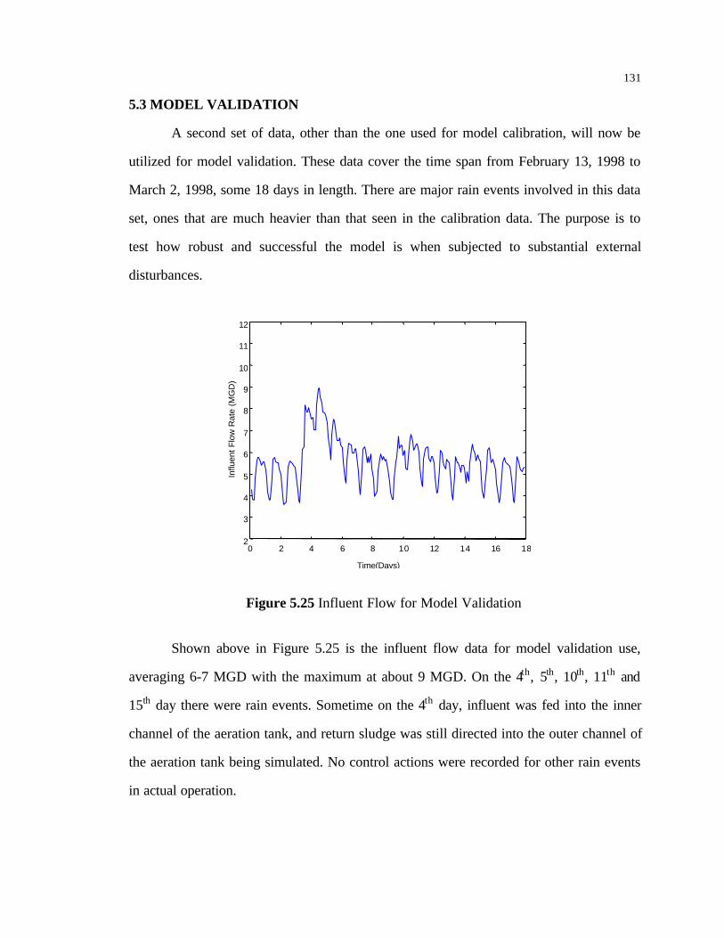
131
5.3 MODEL VALIDATION
A second set of data, other than the one used for model calibration, will now be
utilized for model validation. These data cover the time span from February 13, 1998 to
March 2, 1998, some 18 days in length. There are major rain events involved in this data
set, ones that are much heavier than that seen in the calibration data. The purpose is to
test how robust and successful the model is when subjected to substantial external
disturbances.
0 2 4 6 8 10 12 14 16 18 2 3 4 5 6 7 8 9
10 11 12
Time(Days)
Influ
ent F
low
Rat
e (M
GD
)
Figure 5.25 Influent Flow for Model Validation
Shown above in Figure 5.25 is the influent flow data for model validation use,
averaging 6-7 MGD with the maximum at about 9 MGD. On the 4th, 5th, 10th, 11th and
15th day there were rain events. Sometime on the 4th day, influent was fed into the inner
channel of the aeration tank, and return sludge was still directed into the outer channel of
the aeration tank being simulated. No control actions were recorded for other rain events
in actual operation.
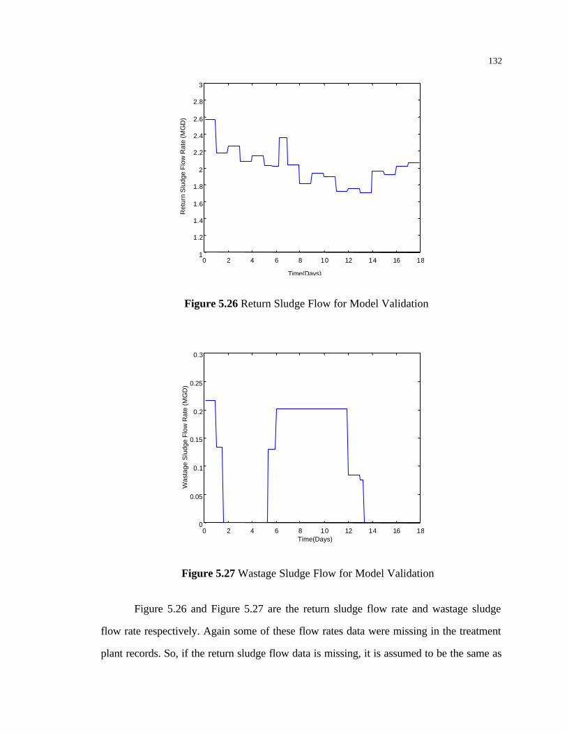
132
0 2 4 6 8 10 12 14 16 18 1 1.2 1.4 1.6 1.8
2 2.2 2.4 2.6 2.8
3
Time(Days)
Ret
urn
Slu
dge
Flo
w R
ate
(MG
D)
Figure 5.26 Return Sludge Flow for Model Validation
0 2 4 6 8 10 12 14 16 18 0
0.05
0.1
0.15
0.2
0.25
0.3
Time(Days)
Was
tage
Slu
dge
Flo
w R
ate
(MG
D)
Figure 5.27 Wastage Sludge Flow for Model Validation
Figure 5.26 and Figure 5.27 are the return sludge flow rate and wastage sludge
flow rate respectively. Again some of these flow rates data were missing in the treatment
plant records. So, if the return sludge flow data is missing, it is assumed to be the same as
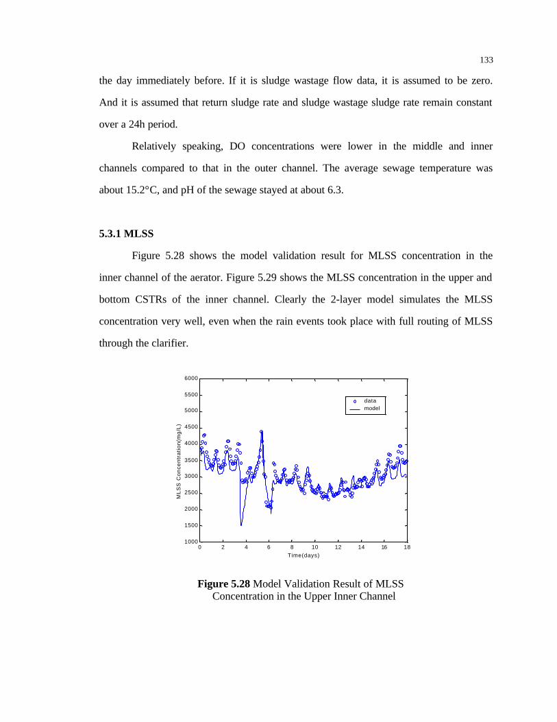
133
the day immediately before. If it is sludge wastage flow data, it is assumed to be zero.
And it is assumed that return sludge rate and sludge wastage sludge rate remain constant
over a 24h period.
Relatively speaking, DO concentrations were lower in the middle and inner
channels compared to that in the outer channel. The average sewage temperature was
about 15.2°C, and pH of the sewage stayed at about 6.3.
5.3.1 MLSS
Figure 5.28 shows the model validation result for MLSS concentration in the
inner channel of the aerator. Figure 5.29 shows the MLSS concentration in the upper and
bottom CSTRs of the inner channel. Clearly the 2-layer model simulates the MLSS
concentration very well, even when the rain events took place with full routing of MLSS
through the clarifier.
0 2 4 6 8 10 12 14 16 181000
1500
2000
2500
3000
3500
4000
4500
5000
5500
6000
Time(days)
ML
SS
Co
nce
ntr
ati
on
(mg
/L)
data model
Figure 5.28 Model Validation Result of MLSS Concentration in the Upper Inner Channel

134
0 2 4 6 8 10 12 14 16 181000
2000
3000
4000
5000
6000
7000
Time(days)
ML
SS
Co
nce
ntr
ati
on
(m
g/L
)
upper layer bottom layer
Figure 5.29 MLSS Concentration in the Upper and Bottom CSTRs of the Inner Channel
The underestimation at the front end is probably due to the time-varying feature
of parameter ‘beta’ (Table 4.2), which is nevertheless assumed constant in the model.
This specific parameter is the fraction of RAS flow dropping into the bottom 1st CSTR
upon entering the aeration tank due to its high density. Its value should be changing with
the number of active aerators in the outer channel, i.e., the more aerators on, the smaller
its value. According to the plant operation records, there were 3 aerators on at the starting
point of the calibration window, while there were 5 operating aerators at the starting point
of the validation window. An alternative smaller value of ‘beta’ was tried, and the
mismatch was minimized.
According to plant records, during certain time period between day 4 and day 5
half of the influent flow was fed directly into the inner channel of the aeration tank being
simulated, with the other half directed to the unused aeration tank. In actual operation the
flow fed into the inner channel might have been less than half, which could have caused
the sharp drop just before day 4 in the simulation result (Figure 5.28). An alternative
value was tested and the speculation was confirmed.

135
The mismatch at the tail end is again attributed to insufficient wastage sludge
flow data. On the very last day sludge was being wasted, but no actual flow data was
recorded. So it is assumed to follow the data of the day immediately before, which might
have not been the case in reality.
All in all, the results above further confirm that 2-layer model is a good
approximation of the real system studied.
5.3.2 Returned Activated Sludge
Figure 5.30 shows the model validation result of RAS concentration in one of the
secondary clarifiers. Obviously the model result misses a peak in data between day 4 and
day 6. The data, however, are quite suspicious, because at that time the sludge was
wasted at a relatively high rate.
0 2 4 6 8 10 12 14 16 180.6
0.8
1
1.2
1.4
1.6
1.8x 10
4
Time(days)
RA
S C
on
cen
tra
tio
n (
mg
/L)
data model
Figure 5.30 Model Validation Result of RAS Concentration in One of the Secondary Clarifiers

136
5.3.3 Sludge Blanket Height
0 2 4 6 8 10 12 14 16 180
5
10
15
Time(days)
SB
L(fe
et)
data model
Figure 5.31 Model Validation Result of Sludge Blanket Height in One of the Secondary Clarifiers
Figure 5.31 shows the model validation result of sludge blanket level. Due to high
flow rate during the rain event, mixed liquor suspended solids are washed out of the
aeration tank into the secondary clarifier (Figure 5.28) such that the sludge blanket level
gradually builds up (as seen in Figure 5.31) if the recycle and waste sludge flow rates are
relatively small, and therefore more suspended solids are seen in the secondary clarifier
effluent (Figure 5.32). Since the measurement of suspended solids in the secondary
effluent is in the unit of FTU, check against model result is impossible.
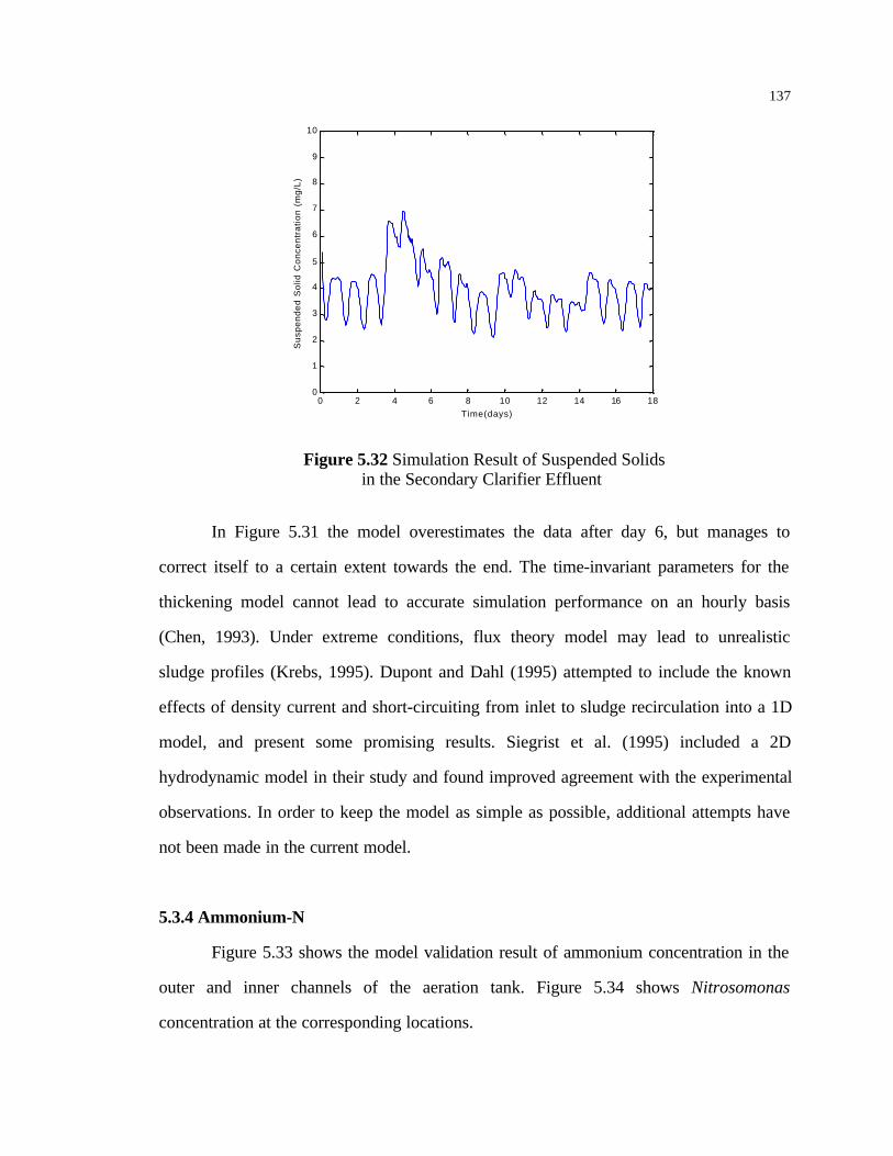
137
0 2 4 6 8 10 12 14 16 180
1
2
3
4
5
6
7
8
9
10
Time(days)
Su
spe
nd
ed
So
lid C
on
cen
tra
tion
(m
g/L
)
Figure 5.32 Simulation Result of Suspended Solids in the Secondary Clarifier Effluent
In Figure 5.31 the model overestimates the data after day 6, but manages to
correct itself to a certain extent towards the end. The time-invariant parameters for the
thickening model cannot lead to accurate simulation performance on an hourly basis
(Chen, 1993). Under extreme conditions, flux theory model may lead to unrealistic
sludge profiles (Krebs, 1995). Dupont and Dahl (1995) attempted to include the known
effects of density current and short-circuiting from inlet to sludge recirculation into a 1D
model, and present some promising results. Siegrist et al. (1995) included a 2D
hydrodynamic model in their study and found improved agreement with the experimental
observations. In order to keep the model as simple as possible, additional attempts have
not been made in the current model.
5.3.4 Ammonium-N
Figure 5.33 shows the model validation result of ammonium concentration in the
outer and inner channels of the aeration tank. Figure 5.34 shows Nitrosomonas
concentration at the corresponding locations.
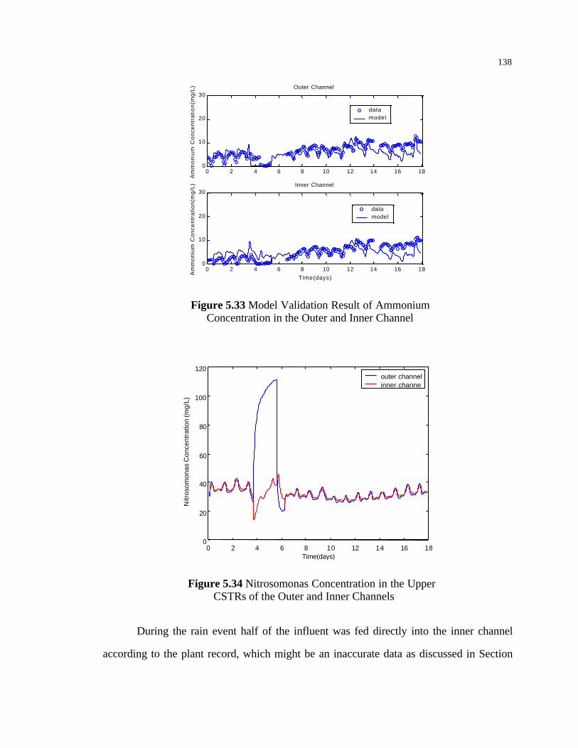
138
0 2 4 6 8 10 12 14 16 180
10
20
30
Am
mo
niu
m C
on
cen
tra
tio
n(m
g/L
) Outer Channel
data model
0 2 4 6 8 10 12 14 16 180
10
20
30
Time(days)
Am
mo
niu
m C
on
cen
tra
tio
n(m
g/L
) Inner Channel
data model
Figure 5.33 Model Validation Result of Ammonium Concentration in the Outer and Inner Channel
0 2 4 6 8 10 12 14 16 18 0
20
40
60
80
100
120
Time(days)
Nitr
osom
onas
Con
cent
ratio
n (m
g/L)
outer channel inner channel
Figure 5.34 Nitrosomonas Concentration in the Upper CSTRs of the Outer and Inner Channels
During the rain event half of the influent was fed directly into the inner channel
according to the plant record, which might be an inaccurate data as discussed in Section

139
5.3.1. This might be the reason the model detects more ammonium downstream than
upstream between day 4 and day 6, as seen in Figure 5.33.
Towards the end of the period, the model underestimates ammonium
concentration in both the outer and inner channels. One possible reason for the
mismatches towards the end of the simulation window is the overestimation of DO in
both the outer and inner channels as seen in Figure 5.35. Data around day 15 are
suspicious because the ammonia probe failed on day 15. Calibration of the probe was
carried out once a day in the early morning. Once a new probe is installed, it needs 24
hours to stabilize (Capital Controls, 1997).
0 2 4 6 8 10 12 14 16 180
2
4
6
8
10
Oxy
ge
n C
on
cen
tra
tion
(mg
/L)
Outer Channel
data model
0 2 4 6 8 10 12 14 16 180
2
4
6
8
10
Time(days)
Oxy
ge
n C
on
cen
tra
tio
n(m
g/L
) Inner Channel
data model
Figure 5.35 DO Concentration in the Upper CSTRs of the Outer and Inner Channels
The consistent overestimation of DO concentration in the outer channel might be
due to the fact that the measurement was taken at the tail end of the aerator, where DO
levels can be expected to be lower than that at the head end of the aerator. Another
explanation for the overestimation is that during the rain event when influent flow is fed

140
directly into the inner channel and the return sludge is still fed into the outer channel, the
number of aerators operating in the outer channel is usually decreased to 2 to keep the
solids in suspension. But this decrease in aerator number might not have been recorded.
5.3.5 Nitrite-N
The following figure shows the simulation results of nitrite in the middle channel
and secondary clarifier effluent. The model largely matches the fairly low nitrite level.
0 2 4 6 8 10 12 14 16 180
0.5
1
1.5
2
Nit
rite
Co
nce
ntr
ati
on
(mg
/L)
Middle Channel
data model
0 2 4 6 8 10 12 14 16 180
0.5
1
1.5
2
Time(days)
Nitr
ite C
once
ntra
tion(
mg/
L)
Clarifier Effluent
data model
Figure 5.36 Model Validation Result of Nitrite Concentration in the Middle Channel and the Secondary Clarifier Effluent
5.3.6 Nitrate-N
Figure 5.37 shows the model validation results of nitrate concentrations in the
middle channel and the secondary clarifier effluent using the parameter values obtained
from model calibration exercise. Obviously, denitrification rates for the calibration data
do not quite apply to the validation data, especially in reference to the top plot in Figure
5.37. This is due to the fact that more aerators were on during the validation data period
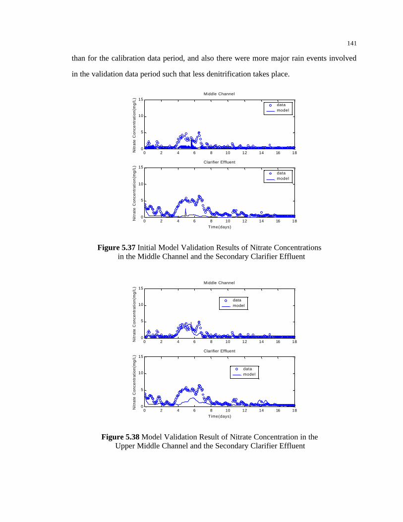
141
than for the calibration data period, and also there were more major rain events involved
in the validation data period such that less denitrification takes place.
0 2 4 6 8 10 12 14 16 180
5
10
15
Nitr
ate
Con
cent
ratio
n(m
g/L)
Middle Channel
data model
0 2 4 6 8 10 12 14 16 180
5
10
15
Time(days)
Nitr
ate
Co
nce
ntr
atio
n(m
g/L
)
Clarifier Effluent
data model
Figure 5.37 Initial Model Validation Results of Nitrate Concentrations in the Middle Channel and the Secondary Clarifier Effluent
0 2 4 6 8 10 12 14 16 180
5
10
15
Nitr
ate
Co
nce
ntr
atio
n(m
g/L
)
Middle Channel
data model
0 2 4 6 8 10 12 14 16 180
5
10
15
Time(days)
Nitr
ate
Con
cent
ratio
n(m
g/L)
Clarifier Effluent
data model
Figure 5.38 Model Validation Result of Nitrate Concentration in the Upper Middle Channel and the Secondary Clarifier Effluent

142
Therefore, smaller denitrification rate values were chosen. Figure 5.38 shows the
model validation result of nitrate concentration in the upper middle channel and
secondary clarifier effluent. The model successfully simulated the surge for nitrate in the
middle channel, however, less so for that in the secondary clarifier effluent. The
underestimation of nitrate concentration in the secondary clarifier (bottom plot in Figure
5.38) can be somehow correlated with overestimation of ammonium concentration in the
inner channel in Figure 5.33. The source of error can also be associated with inaccurate
operational data on the percentage of influent feeding into the inner channel during the
rain events as discussed in Section 5.3.1.
5.3.7 TOC
Figure 5.39 shows the model validation result of TOC concentration in the outer
and inner Channel respectively. The model does a relatively good job in matching the
data. The mismatches in the inner channel from day 3 to about day 5 correlate with
underestimations of DO (as shown in Figure 5.35). Partitioning of the aerator influent
TOC into various constituents could be another source of error, as discussed in Section
5.2.2.
0 2 4 6 8 10 12 14 16 180
20
40
60
TO
C C
once
ntra
tion(
mg/
L)
Outer Channel
data model
0 2 4 6 8 10 12 14 16 180
20
40
60
Time(days)
TO
C C
once
ntra
tion(
mg/
L)
Inner Channel
data model
Figure 5.39 Model Validation Result of TOC Concentration in the Outer and Inner Channel

143
5.3.8 Ortho-Phosphate-P
Figure 5.40 shows the model validation results of phosphorus concentration in the
middle channel and the secondary clarifier effluent. The possible explanation for the
overestimation of ortho-phosphate-P between day 6 to about day 9 is lower organic
loading during the same period of time. The mismatch might have resulted from the slow
rate at which depleted poly-β-hydroxybutyrate (PHB) storage is replenished (Temmink et
al., 1996), as reported in Chapter 2.
0 2 4 6 8 10 12 14 16 180
1
2
3
Ort
ho
-P C
on
cen
tra
tio
n(m
g/L
)
Middle Channel
data model
0 2 4 6 8 10 12 14 16 180
1
2
3
Time(days)
Ort
ho
-P C
on
cen
tra
tio
n(m
g/L
)
Clarifier Effluent
data model
Figure 5.40 Model Validation Result of Phosphorus Concentration in the Upper Middle Channel and Secondary Clarifier Effluent
5.4 PARAMETER ESTIMATION
The parameters in the proposed model were changed on a “trial and error” basis to
achieve the best fit between the results generated by the model and the data obtained
from the sample campaign. No more complicated calibration techniques were adopted
due to large number of parameters in the current model. The final parameter values are
listed in Table 5.1 below, for which the simulation results have already been illustrated in
Sections 5.2 (calibration) and 5.3 (validation).
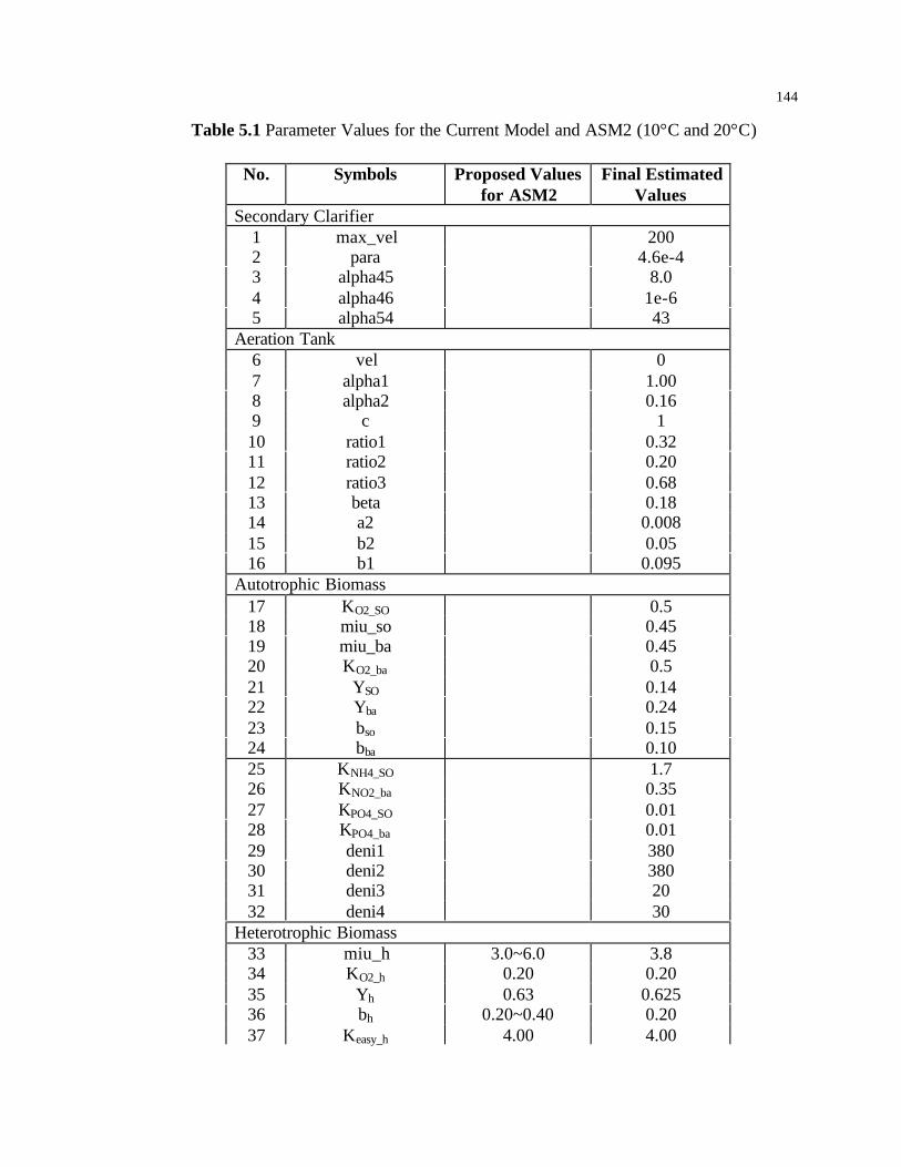
144
Table 5.1 Parameter Values for the Current Model and ASM2 (10°C and 20°C)
No. Symbols Proposed Valuesfor ASM2
Final EstimatedValues
Secondary Clarifier1 max_vel 2002 para 4.6e-43 alpha45 8.04 alpha46 1e-65 alpha54 43
Aeration Tank6 vel 07 alpha1 1.008 alpha2 0.169 c 110 ratio1 0.3211 ratio2 0.2012 ratio3 0.6813 beta 0.1814 a2 0.00815 b2 0.0516 b1 0.095
Autotrophic Biomass17 KO2_SO 0.518 miu_so 0.4519 miu_ba 0.4520 KO2_ba 0.521 YSO 0.1422 Yba 0.2423 bso 0.1524 bba 0.1025 KNH4_SO 1.726 KNO2_ba 0.3527 KPO4_SO 0.0128 KPO4_ba 0.0129 deni1 38030 deni2 38031 deni3 2032 deni4 30
Heterotrophic Biomass33 miu_h 3.0~6.0 3.834 KO2_h 0.20 0.2035 Yh 0.63 0.62536 bh 0.20~0.40 0.2037 Keasy_h 4.00 4.00

145
38 KNO3_h 0.50 0.5039 KNH4_h 0.05 0.0540 Kpo4_h 0.01 0.0141 KNO2_h 0.3242 qfe 1.5~3.0 1.5043 Kfe 20.00 20.00
Phosphorus-accumulating bacteria44 miu_pao 0.67~1.00 0.7045 KO2_PAO 0.20 0.2046 YPAO 0.63 0.62547 bPAO 0.10~0.20 0.1048 bPP 0.10~0.20 0.1049 bpha 0.10~0.20 0.1050 qpp 1.00~1.50 1.5051 qpha 2.00~3.00 3.0052 KNH4_PAO 0.05 0.0553 KPO4_PAO 0.01 0.0154 KNO3_PAO 0.50 0.5055 KA_PAO 4.00 4.0056 KPP 0.01 0.0157 KPHA 0.01 0.0158 Kmax 0.34 0.3459 Kipp 0.02 0.02
Hydrolysis60 Kh 2.00~3.00 2.5061 Kx_h 0.10~0.30 0.1062 eda_NO3 0.60 0.60
Others63 ipbm 0.02 0.0264 fxi 0.10 0.1065 gamma_PO4 0.40 0.4066 gamma_pha 0.20 0.2067 const 868 ratio_so 0.01169 ratio_ba 0.02070 ratio_h 0.01871 ratio_pao 0.0572 ratio_pha 073 ratio_pp 074 ratio_slow 075 percentage_easy 176 percentage_ferment 077 percentage_inert 0

146
5.5 SENSITIVITY ANALYSIS
5.5.1 Sensitivity of Biomass to Initial Conditions
In this section alternative initial concentrations for different kinds of biomasses
are tested to obtain a sense of the characteristic time constants of their dynamic behavior.
Now sensitivity of various categories of biomass to initial conditions will be
tested. Location for each kind of biomass is picked purely at random. For each kind of
biomass their initial concentrations in each channel are taken the same values.
5.5.1.1 Nitrosomonas
0 0.5 1 1.5 2 2.5 3 3.5 4 4.5 510
15
20
25
30
35
40
45
50
Time(days)
Nit
roso
mo
na
s C
on
cen
tra
tio
n (
mg
/L)
Outer Channel
Figure 5.41 Sensitivity of Nitrosomonas to Different Initial Concentrations
Figure 5.41 shows sensitivity of Nitrosomonas to different initial concentrations.
It reaches stable state in less than 1.5 days.

147
5.5.1.2 Nitrobacter
0 0.5 1 1.5 2 2.5 3 3.5 4 4.5 510
20
30
40
50
60
70
80
90
Time(days)
Nitr
ob
act
er
Co
nce
ntr
atio
n (
mg
/L)
Middle Channel
Figure 5.42 Sensitivity of Nitrobacter to Different Initial Concentrations
Figure 5.42 shows sensitivity of Nitrobacter to different initial concentrations. It
reaches stable state in a bit less than 2 days.
5.5.1.3 Heterotroph
0 0.5 1 1.5 2 2.5 3 3.5 4 4.5 510
20
30
40
50
60
70
80
90
Time(days)
Het
erot
roph
Con
cent
ratio
n (m
g/L)
Inner Channel
Figure 5.43 Sensitivity of Heterotroph to Different Initial Concentrations
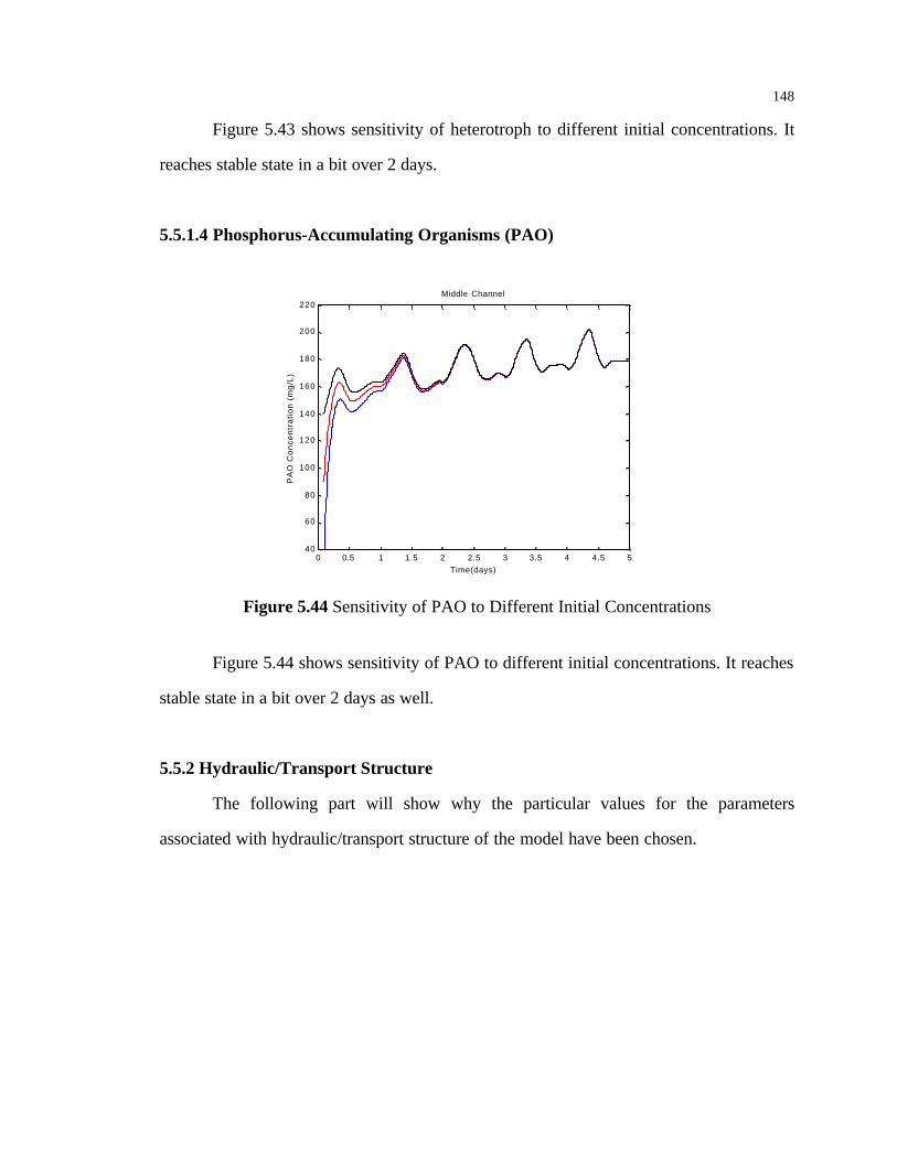
148
Figure 5.43 shows sensitivity of heterotroph to different initial concentrations. It
reaches stable state in a bit over 2 days.
5.5.1.4 Phosphorus-Accumulating Organisms (PAO)
0 0.5 1 1.5 2 2.5 3 3.5 4 4.5 540
60
80
100
120
140
160
180
200
220
Time(days)
PA
O C
on
cen
tra
tio
n (
mg
/L)
Middle Channel
Figure 5.44 Sensitivity of PAO to Different Initial Concentrations
Figure 5.44 shows sensitivity of PAO to different initial concentrations. It reaches
stable state in a bit over 2 days as well.
5.5.2 Hydraulic/Transport Structure
The following part will show why the particular values for the parameters
associated with hydraulic/transport structure of the model have been chosen.

149
5.5.2.1 ‘beta’
0 2 4 6 8 10 12 14 16 182600
2800
3000
3200
3400
3600
3800
4000
4200
4400
Time(days)
ML
SS
Co
nce
ntr
ati
on
(m
g/L
)
Inner Channel
data beta=0 beta=0.15beta=0.18
Figure 5.45 MLSS Concentration in the Inner Channel
‘beta’ is the fraction of return sludge immediately dropping into the bottom CSTR
of the outer channel upon entering the aeration tank. The chosen value for ‘beta’ in the
model is 0.18.
5.5.2.2 ‘alpha1’
0 2 4 6 8 10 12 14 16 182600
2800
3000
3200
3400
3600
3800
4000
4200
4400
Time(days)
ML
SS
Co
nce
ntr
ati
on
(m
g/L
)
Inner Channel
data alpha1=0.95alpha1=0.98alpha1=1
Figure 5.46 MLSS Concentration in the Inner Channel
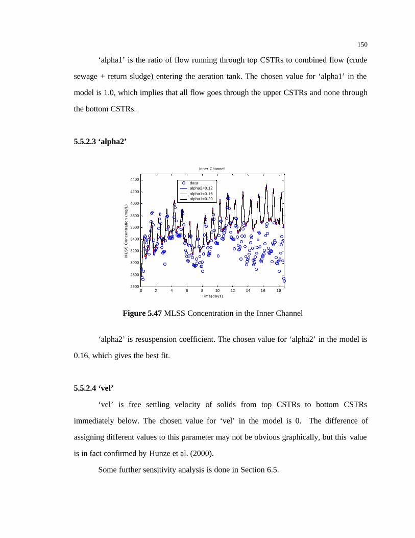
150
‘alpha1’ is the ratio of flow running through top CSTRs to combined flow (crude
sewage + return sludge) entering the aeration tank. The chosen value for ‘alpha1’ in the
model is 1.0, which implies that all flow goes through the upper CSTRs and none through
the bottom CSTRs.
5.5.2.3 ‘alpha2’
0 2 4 6 8 10 12 14 16 182600
2800
3000
3200
3400
3600
3800
4000
4200
4400
Time(days)
ML
SS
Co
nce
ntr
ati
on
(m
g/L
)
Inner Channel
data alpha2=0.12alpha1=0.16alpha1=0.20
Figure 5.47 MLSS Concentration in the Inner Channel
‘alpha2’ is resuspension coefficient. The chosen value for ‘alpha2’ in the model is
0.16, which gives the best fit.
5.5.2.4 ‘vel’
‘vel’ is free settling velocity of solids from top CSTRs to bottom CSTRs
immediately below. The chosen value for ‘vel’ in the model is 0. The difference of
assigning different values to this parameter may not be obvious graphically, but this value
is in fact confirmed by Hunze et al. (2000).
Some further sensitivity analysis is done in Section 6.5.

151
5.6 CONCLUSIONS
The model has been evaluated against two sets of field data retrieved from the
same sampling campaign described in Chapter 3. The first set of data is used for model
calibration. The second study deals with model validation. Evaluation of the model
against both sets of data demonstrates the model’s capability to simulate the nutrient
removal processes in an activated sludge system. However, it is also found that there are
flaws in the model structure, in particular, with respect to biological phosphorus removal.
Yet, since they are not found to be critical, the model can reasonably be used for the
assessment of operational control strategies in the next Chapter.

152
CHAPTER 6
DEVELOPMENT AND EVALUATION OF PROCESS
CONTROL STRATEGIES
6.1 INTRODUCTION
Various control strategies for the activated sludge process have been reviewed in
Chapter 2. A dynamic model was then developed in Chapter 4 and the results of its
evaluation against field data were presented in Chapter 5. Therefore, we are now in a
position to explore the application of this model in the development and evaluation of
process control strategies for the activated sludge system. The strategies to be studied in
this Chapter are for short-term operational control under transient variations in the
influent, especially for the case of storm run-off events.
This Chapter is organized as follows. Overall design of the assessment is
specified in section 6.2, including control objectives and selection of the criteria for
evaluation of the various strategies. A comprehensive set of control algorithms is then set
out in section 6.3. The results of testing these algorithms are presented in section 6.4.
6.2 SPECIFICATION OF THE ASSESSMENT
6.2.1 Configuration of The Activated Sludge Process
A typical conventional activated sludge plant configuration to be studied in this
Chapter is basically the same as that at the Athens Wastewater Treatment Facility No. 2.
All the influent flow passes through the entire plant without any diversions of excess
flow. By doing so, the effects of storm events and their control can be fully revealed. The
aeration tank has three circular channels. Both crude sewage and returned activated
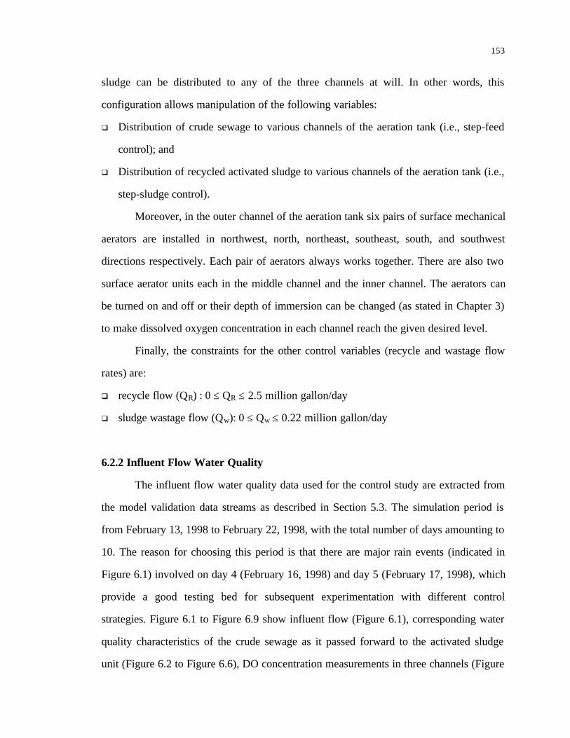
153
sludge can be distributed to any of the three channels at will. In other words, this
configuration allows manipulation of the following variables:
q Distribution of crude sewage to various channels of the aeration tank (i.e., step-feed
control); and
q Distribution of recycled activated sludge to various channels of the aeration tank (i.e.,
step-sludge control).
Moreover, in the outer channel of the aeration tank six pairs of surface mechanical
aerators are installed in northwest, north, northeast, southeast, south, and southwest
directions respectively. Each pair of aerators always works together. There are also two
surface aerator units each in the middle channel and the inner channel. The aerators can
be turned on and off or their depth of immersion can be changed (as stated in Chapter 3)
to make dissolved oxygen concentration in each channel reach the given desired level.
Finally, the constraints for the other control variables (recycle and wastage flow
rates) are:
q recycle flow (QR) : 0 ≤ QR ≤ 2.5 million gallon/day
q sludge wastage flow (Qw): 0 ≤ Qw ≤ 0.22 million gallon/day
6.2.2 Influent Flow Water Quality
The influent flow water quality data used for the control study are extracted from
the model validation data streams as described in Section 5.3. The simulation period is
from February 13, 1998 to February 22, 1998, with the total number of days amounting to
10. The reason for choosing this period is that there are major rain events (indicated in
Figure 6.1) involved on day 4 (February 16, 1998) and day 5 (February 17, 1998), which
provide a good testing bed for subsequent experimentation with different control
strategies. Figure 6.1 to Figure 6.9 show influent flow (Figure 6.1), corresponding water
quality characteristics of the crude sewage as it passed forward to the activated sludge
unit (Figure 6.2 to Figure 6.6), DO concentration measurements in three channels (Figure

154
6.7), MLSS concentration measurement in the inner channel (Figure 6.8), and sludge
blanket level measurement in one of the secondary clarifies (Figure 6.9). Figure 6.7 to
Figure 6.9 complete the picture of actual operating conditions.
Figure 6.1 Influent Flow
Figure 6.2 Influent Ammonium Concentrations
0 1 2 3 4 5 6 7 8 9 102
3
4
5
6
7
8
9
10
Time(day)
Influ
ent F
low
(MG
D)
0 1 2 3 4 5 6 7 8 9 100
5
10
15
20
25
Time(day)
Am
mon
ium
Con
cent
ratio
n (m
g/L)
Rain Events

155
Figure 6.3 Influent Nitrite Concentrations
Figure 6.4 Influent Nitrate Concentrations
0 1 2 3 4 5 6 7 8 9 100
0.005
0.01
0.015
0.02
0.025
0.03
0.035
0.04
0.045
0.05
Time(day)
Nitr
ite C
once
ntra
tion
(mg/
L)
0 1 2 3 4 5 6 7 8 9 100
0.2
0.4
0.6
0.8
1
1.2
1.4
1.6
1.8
2
Time(day)
Nitr
ate
Con
cent
ratio
n (m
g/L)

156
Figure 6.5 Influent TOC Concentrations
Figure 6.6 Influent Ortho-phosphate-P Concentrations
Obviously, influent concentrations of ammonium, TOC and orthophosphate-P
decrease during the rain events due to the dilution effects. However, influent nitrite and
0 1 2 3 4 5 6 7 8 9 100
5
10
15
20
25
30
35
40
45
50
Time(day)
TOC
Con
cent
ratio
n (m
g/L)
0 1 2 3 4 5 6 7 8 9 100
1
2
3
4
5
6
7
8
9
Time(day)
Orth
opho
spho
rus
Con
cent
ratio
n (m
g/L)

157
nitrate concentrations increase during the storm events, something which can be
attributed to many factors, including acute high loadings (Alleman, 1984; Henze, 1995).
0 1 2 3 4 5 6 7 8 9 100
1
2
3
4
5
6
7
8
Time(days)
DO
Con
cent
ratio
n(m
g/L)
outer channel middle channelinner channel
Figure 6.7 DO Concentration Measurements in All Three Channels
0 1 2 3 4 5 6 7 8 9 101000
1500
2000
2500
3000
3500
4000
4500
5000
5500
6000
Time(days)
ML
SS
Co
nce
ntr
ati
on
(mg
/L)
Figure 6.8 MLSS Concentration Measurement in Inner Channel

158
0 1 2 3 4 5 6 7 8 9 10
0
2
4
6
8
10
12
Time(days)
SB
L(fe
et)
Figure 6.9 Sludge Blanket Level Measurement in One Secondary Clarifier
During the storm events, DO concentrations increase in all three channels (Figure
6.7) due to elevated turbulency. Mixed liquor suspended solids, however, are flushed out
of the aeration tank (Figure 6.8) because of the hydraulic surge, such that sludge begins
to build up in the secondary clarifier subsequently (Figure 6.9).
6.2.3 Objectives and Constraint Functions For Process Control Strategies
The following two control objectives will be used in the study:
q Ensure that the plant satisfies the regulatory effluent standards for suspended solids
(SS), and ammonium, and specified standards for nitrite, nitrate, TOC and ortho-
phosphate-P;
q Improve the effluent water quality as much as possible under the conditions provided.
The objectives above can be expressed in the following mathematical forms such
that the settings of the manipulated control variables (returned sludge flow, wastage flow,
etc.) during the simulation can be chosen on the basis of their satisfaction.

159
q Effluent in compliance
where,
Yeff−Simulated effluent water quality, and
Ystd−Desired effluent standard over the period of T.
For SS and ammonium, the current regulatory effluent standards are 30 and 17
mg/L respectively. While the effluent standards for nitrite, nitrate, TOC and
ortho-phosphate-P to be used in this control study are assumed to take the
values of 0.2 (Effler et al., 1996), 2.5 (Orth et al., 1988), 30 (Orth et al., 1988),
and 2 mg/L (Werumeus Buning et al., 1991) respectively;
T−Sampling period over which the actual behavior of the process is checked against
its desired behavior.
q Maximum water quality
where,
Yss,YNH3,YTOC,YP,YNO2,YNO3−Simulated effluent water quality for the suspended
solids, ammonium, TOC, ortho-phosphate-P, nitrite, and nitrate respectively;
w1, w2, w3, w4, w5, w6−Weighting coefficients. In this study, SS and ammonium
are given priority over TOC, ortho-phosphate-P, nitrite and nitrate, so that w1, w2,
w3, w4, w5, and w6 are chosen as 0.3, 0.3, 0.1, 0.1, 0.1, and 0.1 respectively.
The formulation immediately above is based on Chen’s work (1993), but
including more water quality indicators, specifically TOC, ortho-phosphate-P, nitrite and
nitrate.
∫ ≤=T
stdeff YdtYT
P0
1
1
})*6*5
*4*3*2*1({
3,
3
2,
2
0 ,,3,
3
,2
dtYY
wYY
w
YY
wYY
wYY
wYY
wMinP
NOstd
NO
NOstd
NO
T
Pstd
P
TOCstd
TOC
NHstd
NH
SSstd
SS
++
+++= ∫

160
For these two objectives, the control variables are changed on an hourly basis,
except the step-feed and step-sludge controls as discussed below, because effluent quality
is more easily influenced by relatively fast transient disturbances. More detailed
discussion of the design of the control algorithms will be continued in section 6.3.
6.2.4 Criteria for Evaluation of Controlled Plant Performance
It is hard to differentiate between the performances of the various control
strategies in the context of the entire sewage plant management without simulating the
behavior of the whole treatment plant and the receiving water quality. Such a more
complete assessment is beyond the scope of this dissertation, although extensive work
has been done on evaluating the impacts of effluent discharges on receiving water quality
(Reda,1993; Duchesne et al., 2000; Schutze et al., 2000). In this control study, evaluation
of the controlled plant performance will be based primarily on the performance of the
activated sludge process itself. For each strategy tested, the following summaries will be
used for comparative assessment:
q Maximum concentrations of SS, ammonium, nitrite, nitrate, TOC, and ortho-
phosphate-P in the secondary clarifier effluent over the storm period;
q Average effluent loadings of SS, ammonium, nitrite, nitrate, TOC, and ortho-
phosphate-P in the secondary clarifier effluent over the storm period;
q Graphs of the effluent and activated sludge process responses, including the effluent
SS, effluent ammonium, mixed liquor suspended solid concentration, and sludge
blanket height.
The threshold values mentioned above are set at 30, 17, 0.2, 2.5, 30, and 2 mg/L
for SS, ammonium, nitrite, nitrate, TOC and ortho-phosphate-P respectively. They are
also approximately the maximum effluent concentrations found during normal operation
at Athens wastewater treatment facility No.2.

161
6.3 DETAILED SPECIFICATION OF THE CONTROL ALGORITHMS
Many combinations of the control strategies presented in Chapter 2 might be used
for exploring the operational flexibility of the activated sludge process. Such an
exhaustive analysis, however, would be beyond the scope of this dissertation. Only the
practical strategies and those clearly demonstrating both the potential of the model and
the importance of simple control actions will be examined herein.
More specifically, the following four groups of control strategies are to be
investigated for the control of storm disturbances.
q Conventional Control
• Returned sludge flow rate (QR) is manipulated in proportion to the influent flow
rate (Qin);
• Sludge wastage flow rate (Qw) is chosen as a function of the calculated sludge
age. Sludge age is calculated as the total amount of sludge in the system divided
by the rate of sludge loss from the system. The equation is defined as follows
(Grady et al., 1999).
eewws XQXQ
VXt
+=
where,
ts−Sludge age;
V−Volume of liquid in the aeration tank;
X−MLSS concentration in the aeration tank;
Qw−Sludge wastage rate;
Xw−Sludge concentration in the sludge wastage flow;
Qe−Secondary effluent flow;
Xe−Suspended solid concentration in the secondary effluent;

162
q Feedback Control
• QR is changed as a function of the effluent quality;
• Qw is similarly manipulated as QR.
q Advanced Control
• Step Feed
• Step Sludge
q DO Set-Point Control
6.3.1 Base Case Control
One simulation run is essential to provide a reference point for comparisons
among the various control strategies. Return sludge flow and wastage sludge flow data
used in this simulation run are the same as those in the actual operation of the Athens
Wastewater Treatment Facility No. 2. Figure 6.10 shows return sludge flow from one of
the three secondary clarifiers for the entire simulation window. Due to the limited number
of facilities in EPCL, only this specific clarifier was monitored during the sampling
campaign described in Chapter 3. During actual plant operation return sludge flow in
each secondary clarifier (three in total) is adjusted according to the sludge blanket level in
the specified clarifier based purely on experience. For instance, if the sludge blanket level
is above 10 feet, return sludge flow is increased by about 0.10MGD. Conversely, if the
sludge blanket level is below 2 feet, return sludge flow is decreased by about 0.10 MGD.
Shown in Figure 6.11, on the other hand, is the combined return sludge flow from all
three secondary clarifiers.

163
0 2 4 6 8 10 12 14 16 18 0.4
0.5
0.6
0.7
0.8
0.9
1
Time(days)
One Secondary Clarifier
Ret
urne
d S
ludg
e F
low
(M
GD
)
Figure 6.10 Returned Sludge Flow Rate Data During the Entire Simulation Period from One of the Secondary Clarifiers
Figure 6.10 Returned Sludge Flow Rate Data During the Entire Simulation Period
Figure 6.11 Combined Returned Sludge Flow Rate Data from All Three Secondary Clarifiers
0 1 2 3 4 5 6 7 8 9 10 1.2
1.4
1.6
1.8
2
2.2
2.4
2.6
2.8
3
Time(day)
Ret
urne
d S
ludg
e F
low
(M
GD
)

164
Figure 6.11 Wasted Sludge Flow Rate Data
During the Entire Simulation Period
Figure 6.12 Sludge Wastage Flow
Figure 6.12 shows the actual manipulation of the sludge wastage flow. Processing
of waste sludge is operated at the Athens Wastewater Treatment Facility No.2 only four
days a week, normally from 5:00am to 4:00pm, Monday through Thursday. The sludge
wastage processing machines are stopped at times other than that specified. Also there
exists a limitation on the sludge wastage capacity. When sludge builds up in the
secondary clarifier and an elevated sludge wastage is desirable, the sludge-processing
sector in the treatment plant may therefore not be able to accommodate this need.
Half of the influent flow was fed directly into the inner channel of aeration tank
No. 2 with the other half fed into the inner channel of aeration tank No.1 at 3:00pm on
February 16, 1998. On February 19, 1998 at 8:15am all the influent flow began to be
channeled through the outer channel of aeration tank No.2 again. Thereafter normal
operation resumed.
Shown in Figure 6.13 is the actual number of active aerators in the outer channel
during the simulation period. There are six pairs of aerators in the outer channel of the
aeration tank, and two each in the middle and inner channel. The aerators in the middle
0 1 2 3 4 5 6 7 8 9 100
0.05
0.1
0.15
0.2
0.25
0.3
Time(day)
Was
ted
Slu
dge
Flow
(M
GD
)
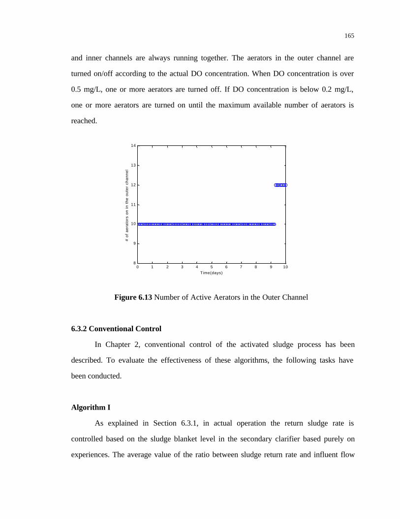
165
and inner channels are always running together. The aerators in the outer channel are
turned on/off according to the actual DO concentration. When DO concentration is over
0.5 mg/L, one or more aerators are turned off. If DO concentration is below 0.2 mg/L,
one or more aerators are turned on until the maximum available number of aerators is
reached.
0 1 2 3 4 5 6 7 8 9 108
9
10
11
12
13
14
Time(days)
# of
aer
ator
s on
in t
he o
uter
cha
nnel
Figure 6.13 Number of Active Aerators in the Outer Channel
6.3.2 Conventional Control
In Chapter 2, conventional control of the activated sludge process has been
described. To evaluate the effectiveness of these algorithms, the following tasks have
been conducted.
Algorithm I
As explained in Section 6.3.1, in actual operation the return sludge rate is
controlled based on the sludge blanket level in the secondary clarifier based purely on
experiences. The average value of the ratio between sludge return rate and influent flow

166
rate, however, is about 0.28 even though it was not in fact so manipulated during the
storm event. In this algorithm the sludge return rate (QR) is controlled in proportion to the
influent flow rate Qin, i.e., QR=k1*Qin. The following three cases are tested:
q Strategy 1: QR = 0.25 * Qin
q Strategy 2: QR = 0.35 * Qin
q Strategy 3: QR = 0.42 * Qin
Algorithm II
Sludge wastage rate (Q w) can be controlled using the sludge age. In actual
operation the sludge wastage flow stayed zero during the storm event for the reason
explained in Section 6.3.1. Conventional activated sludge has a sludge age of 3-4 days,
and has good settling properties. However, at a sludge age greater than 6 day there is a
reduction in settleability (Gray, 1990). The following three cases are therefore tested:
q Strategy 4: Qw is adjusted to give a sludge age of 3 days
q Strategy 5: Qw is adjusted to give a sludge age of 4 days
q Strategy 6: Qw is adjusted to give a sludge age of 12 days
6.3.3 Feedback Control
Although conventional feedback control may include what is called proportional
(P), integral (I), and derivative (D) action (Olsson and Newell, 1999), only proportional
feedback controllers are considered in this study. Again, as for the conventional controls
in section 6.3.2, the sludge return rate (QR) and sludge wastage (Qw) rate are considered
as the only control variables.
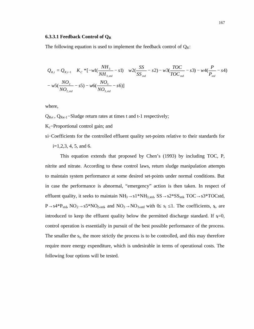
167
6.3.3.1 Feedback Control of QR
The following equation is used to implement the feedback control of QR:
where,
QR,t , QR,t-1−Sludge return rates at times t and t-1 respectively;
Kc−Proportional control gain; and
si−Coefficients for the controlled effluent quality set-points relative to their standards for
i=1,2,3, 4, 5, and 6.
This equation extends that proposed by Chen’s (1993) by including TOC, P,
nitrite and nitrate. According to these control laws, return sludge manipulation attempts
to maintain system performance at some desired set-points under normal conditions. But
in case the performance is abnormal, “emergency” action is then taken. In respect of
effluent quality, it seeks to maintain NH3→s1*NH3,std, SS→s2*SSstd, TOC→s3*TOCstd,
P→s4*Pstd, NO2→s5*NO2,std, and NO3→NO3,std with 0≤ si ≤1. The coefficients, si, are
introduced to keep the effluent quality below the permitted discharge standard. If si=0,
control operation is essentially in pursuit of the best possible performance of the process.
The smaller the si, the more strictly the process is to be controlled, and this may therefore
require more energy expenditure, which is undesirable in terms of operational costs. The
following four options will be tested.
)]6(6)5(5
)4(4)3(3)2(2)1(1[*
,3
3
,2
2
,3
31,,
sNONO
wsNONO
w
sPP
wsTOCTOC
wsSSSS
wsNHNH
wKQQ
stdstd
stdstdstdstdCtRtR
−−−−
−−−−−+−−+= −

168
Algorithm III
q Strategy 7: Kc = -5e-3, s1 = s2 = s3 = s4 = s5 = s6 = 0.8
q Strategy 8: Kc = -1e-4, s1 = s2 = s3 = s4 = s5 = s6 = 0.8
q Strategy 9: Kc = -1e-3, s1 = s2 = s3 = s4 = s5 = s6 = 0.5
6.3.3.2 Feedback Control of Qw
Feedback control of Qw is based on a principle similar to that described in section
6.3.3.1 for QR. The control rules are thus applied to Qw as shown in the following
equation.
Obviously, the control gain Kc will be different. So we have the following options.
Algorithm IV
q Strategy 10: Kc = - 0.001, s1 = s2 = s3 = s4 = s5 = s6 = 0.8
q Strategy 11: Kc = -0.003, s1 = s2 = s3 = s4 = s5 = s6 = 0.8
q Strategy 12: Kc = -0.003, s1 = s2 = s3 = s4 = s5 = s6 = 0.6
6.3.4 Advanced Control
In Chapter 2 we noted that operation of the activated sludge process can be
enhanced by implementing step-feed control, especially when the system experiences
abnormal short-term influent shocks (Funamizu et al., 1997). This and other options are
now considered. Step-sludge and step-feed are both implemented only during the storm
event.
)]6(6)5(5
)4(4)3(3)2(2)1(1[*
,3
3
,2
2
,3
31,,
sNONO
wsNONO
w
sPP
wsTOCTOC
wsSSSS
wsNHNH
wKQQ
stdstd
stdstdstdstdCtwtw
−+−+
−+−+−−−+= −

169
6.3.4.1 Step Sludge
In this algorithm, the influent flow still enters the aeration tank from the outer
channel, while the returned activated sludge flow is split between outer, middle, and inner
channels. In other words, each channel receives a portion of the total returned sludge
flow, and the sum of the returned sludge fed to each channel amounts to the total returned
sludge flow pumped from the bottom of the secondary clarifiers.
Algorithm V
q Strategy 13: w7 = 0.80, w8 = 0.20, w9 = 0
q Strategy 14: w7 = 0.60, w8 = 0.20, w9 = 0.20
q Strategy 15: w7 = 0.10, w8 = 0.20, w9 = 0.70
where,
w7−Fraction of returned sludge entering the outer channel of the aeration tank;
w8−Fraction of returned sludge entering the middle channel;
w9−Fraction of returned sludge entering the inner channel.
6.3.4.2 Step Feed
In this algorithm, the returned sludge flow enters the aeration tank from the outer
channel, while influent flow is split between outer, middle, and inner channels. In other
words, each channel receives a portion of the influent flow. And the sum of influent flow
fed to each channel amounts to the influent flow entering the aeration tank.
Algorithm VI
q Strategy 16: w10 = 1.00, w11 = 0, w12 = 0
q Strategy 17: w10 = 0.60, w11 = 0.20, w12 = 0.20
q Strategy 18: w10 = 0.20, w11 = 0.20, w12 = 0.60
q Strategy 19: w10 = 0, w11 = 0, w12 = 1.00

170
where,
w10−Fraction of influent flow entering the outer channel;
w11−Fraction of influent flow entering the middle channel;
w12−Fraction of influent flow entering the inner channel.
6.3.5 DO Set-point Control
The purpose of oxygen control is to keep DO profile in the aeration tank at a
desired level such that biochemical reaction would not be downgraded. Many papers
have reported on DO set-point control by adjusting air compressor flow rate (Buhr et al.,
1984; Healey, 1989; Olsson and Newell, 1999). Model based DO set-point control by
turning on and off surface aerators is achieved in a manner similar to airflow control as
suggested by Olsson and Newell (1999).
The error between the DO set-point, SO,SP , and the true DO value, SO, is defined as:
e= SO,SP-So (6.1)
The controller should work so that the error will approach zero. Therefore it is prescribed
that the error should obey the differential equation:
edtde
−= (6.2)
Then take the derivative of Equation 6.1 assuming that DO set-point is constant.
dtdS
SSdtd
dtde O
OSPO −=−= )( , (6.3)
Combining equation 6.2, equation 6.3, and DO dynamics listed in Table 4.3, the
number of aerators needed to keep the desired DO level can be deduced. For instance, the

171
number of aerators needed in the outer channel (denoted as ‘n1’) as a result of the DO
controller is derived as follows:
)1(*)1(
)1(*
)1(
)1(*
)1(
)1(*
)1(
)1(**)
11(
)1(*)1(
)1(*
)1(
)1(*
)1(
)1(**)14.11(
)1(*)1(
)1(*
)1(
)1(*
)1(
)1(**)
43.31(
)1(*)1(*)([1
__4_4
_4
_4_4
_4
_2_2
_2
__
_
__4_4
_4
_2_2
_2
_2_2
_2
__4_4
_4
_2_2
_2
_4_4
_4
1
_2_21
upperHupperPOHPO
upperPO
upperNHHNH
upperNH
upperOHO
upperO
uppereasyHeasy
uppereasyH
H
upperbaupperPObaPO
upperPO
upperNObaNO
upperNO
upperObaO
upperOba
ba
upperSOupperPOSOPO
upperPO
upperOSOO
upperO
upperNHSONH
upperNHSO
SO
upper
bottomOresusupperOdabove
XSK
S
SK
S
SK
S
SK
S
Y
XSK
S
SK
S
SK
S
Y
XSK
S
SK
S
SK
S
Y
V
SQSQQen
++
++−−
+
++−−
+
++−−
++−−=
µ
µ
µ
Although DO control is widely used and an accuracy of 0.2mg/L was reported 20
years ago (Ryder, 1972), the set-point of the DO level is quite system-specific and mostly
in the range of 0.5-1.5 mg/L (Ryder, 1972). In this DO set-point control study, the
following options will be tested:
)](*/[)]1(*
)1(/)1(
)1(/)1(*
)1(/)1(
)1(/)1(*
)1(
)1(*
)1(
)1(**
)1(*)1(/)1(
)1(/)1(*
)1(
)1(*
)1(
)1(*
)1(
)1(**)
11(
,_
__
__
__
__
_4_4
_4
_2_2
_2
___
__
_44
_4
_4_4
_4
_2_2
_2
OSPOupperPAO
upperPAOupperPPMAXIPP
upperPAOupperPPMAX
PHAupperPAOupperPHA
upperPAOupperPHA
PAOPOupperPO
upperPO
PAOOupperO
upperOPPPHA
upperPAOupperPAOupperPHAPHA
upperPAOupperPHA
upperPOPO
upperPO
upperNHpaoNH
upperNH
upperOPAOO
upperOPAO
PAO
SSconstX
XXKK
XXK
KXX
XX
KS
S
KS
Sq
XXXK
XX
SK
S
SK
S
SK
S
Y
−
−+
−
+
+++
++
++−−
γ
µ

172
Algorithm VII
q Strategy 20: SO,SP = 1.0
q Strategy 21: SO,SP = 1.5
q Strategy 22: SO,SP = 5.0
DO set-point as high as 5.0 mg/L is chosen to find out the possible scale of
nitrification improvement and associated energy requirement.
For all the 21 control strategies listed above, the control actions are taken 2 hours
before the storm events start, and ceased 2 hours after the storm events subside. No
control is exercised before and after the event. The time before the event indicates
‘normal operation’, while the simulation window after the storm event could possibly
show the impact on the treatment system in the aftermath of the storms. Also for each
control strategy tested, other than step-feed and step-sludge, during the storm event all
influent flow is still fed into the outer channel (not into the inner channel as in the base
case) and the same for the return sludge flow for the ease of comparing different control
strategies.
6.4 SIMULATION RESULTS AND EVALUATION OF CONTROL STRATEGIES
The results to be presented here have to be selective. The discussion is oriented
towards comparison of the various control strategies and demonstration of the operational
flexibility of the activated sludge process.
Table 6.1 gives summary statistics of the simulation results for the control
strategies tested. Their detailed discussion is presented below.
6.4.1 Conventional Control
6.4.1.1 Control of QR in Proportion to Qin (strategies 1 to 3)
Control of QR in proportion to Qin has both advantages and disadvantages relative
to the base case. From the results of strategies 1-3, it is apparent that ratio control of

173
return sludge rate is better at reducing the average effluent mass loads of ammonium,
nitrate, TOC, and ortho-phosphate-P than the base case. Yet it increases the average
effluent mass loads of SS (see Table 6.1).
0 1 2 3 4 5 6 7 8 9 100
2
4
6
8
10
12
14
16
18
Time(days)
TO
C C
once
ntra
tion
(mg/
L)base case strategy 1strategy 2strategy 3
Figure 6.14 TOC Concentration in the Secondary Clarifier Effluent
0 1 2 3 4 5 6 7 8 9 1020
30
40
50
60
70
80
90
100
110
120
Time(days)
He
tero
tro
ph
Co
nce
ntr
atio
n (
mg
/L)
Inner Channel
base case strategy 1strategy 2strategy 3
Figure 6.15 Heterotroph Concentration in the Upper Inner Channel

174
0 1 2 3 4 5 6 7 8 9 100
0.5
1
1.5
2
2.5
3
Time(days)
Fe
rme
nta
tio
n P
rod
uct
s (m
g/L
)
Inner Upper Channel
base case strategy 1strategy 2strategy 3
Figure 6.16 Fermentation Products Concentration in the Upper Inner Channel
0 1 2 3 4 5 6 7 8 9 100
2
4
6
8
10
12
14
16
18
Time(days)
Ea
sily
Bio
de
gra
da
ble
Su
bst
an
ce (
mg
/L)
Inner Upper Channel
base case strategy 1strategy 2strategy 3
Figure 6.17 Easily Biodegradable Substance Concentration in the Upper Inner Channel
Figure 6.14 shows the TOC concentration profiles in the secondary clarifier
effluent under base-case and strategies 1-3 controls. Obviously, the effluent TOC

175
concentrations are consistently lower than the base case during the storm by
implementing any of strategies 1-3. Figure 6.15 shows heterotroph concentration in the
upper inner channel with different control strategies (strategy 1-3). Figure 6.16 shows
fermentation product concentrations in the upper inner channel. And those curves shown
in Figure 6.17 are easily biodegradable substance concentrations at the same location.
Even though heterotroph concentrations in the inner upper channel for the base
case are higher from day 4.5 to day 6.5 relative to strategy 1-3 (Figure 6.15),
concentrations of fermentation products and easily biodegradable substances at the same
location are consistently higher (Figure 6.16 and Figure 6.17), which therefore causes
higher effluent TOC mass load in the secondary clarifier effluent for the base case (Table
6.1). Worthy of mention is that TOC is modeled as the combination of easily
biodegradable substance, fermentation products, and inert product, which last turns out to
be zero from model calibration (‘percentage-inert’ in Table 5.1).
0 1 2 3 4 5 6 7 8 9 101000
1500
2000
2500
3000
3500
4000
4500
5000
5500
6000
Time(days)
ML
SS
Co
nce
ntr
ati
on
(m
g/L
)
Inner Channel
base case strategy 1strategy 2strategy 3
Figure 6.18 MLSS Concentration in the Upper Inner Channel

176
0 1 2 3 4 5 6 7 8 9 100
2
4
6
8
10
12
14
Time(days)
Slu
dge
blan
ket
leve
l (fe
et)
base case strategy 1strategy 2strategy 3
Figure 6.19 Sludge Blanket Level in One Secondary Clarifier
0 1 2 3 4 5 6 7 8 9 100
5
10
15
Time(days)
Su
spe
nd
ed
so
lids
(mg
/L)
Secondary Clarifier Effluent
base case strategy 1strategy 2strategy 3
Figure 6.20 Suspended Solid Concentration in the Secondary Clarifier Effluent
However, caution should be taken in applying ratio control of QR as far as the
behavior of the sludge blanket is concerned. The more the sludge is returned to the
aeration tank, the larger the mixed liquor concentration in the aeration tank (Figure 6.18).

177
Such circumstances will clearly leave more sludge in the clarifier (Figure 6.19), so that
the risk of sludge overflow is greater (Figure 6.20).
In summary, ratio control of return sludge rate could achieve a better performance
in effluent mass loadings, and a good maintenance of the sludge in the aeration tank
during storm events, but it could lead to deterioration of effluent SS and an increased risk
of sludge overflow.
6.4.1.2 Sludge Age Control (strategies 4 to 6)
The effect of sludge age control through the wastage of sludge (QW) during the
storm event does not prove to be a better strategy than base-case control in terms of
effluent water quality indicators such as ammonium, nitrite, nitrate, and ortho-phosphate-
P (Table 6.1).
0 1 2 3 4 5 6 7 8 9 100
1
2
3
4
5
6
7
8
Time(days)
Am
mo
niu
m C
on
cen
tra
tio
n (
mg
/L)
Secondary Clarifier Effluent
base case strategy 4strategy 5strategy 6
Figure 6.21 Ammonium Concentration in the Secondary Clarifier Effluent

178
0 1 2 3 4 5 6 7 8 9 1020
25
30
35
40
45
50
Time(days)
Nit
roso
mo
na
s C
on
cen
tra
tio
n (
mg
/L)
Inner Upper CSTR
strategy 4strategy 5strategy 6
Figure 6.22 Nitrosomonas Concentration in the Inner Upper CSTR
Also the benefit of implementing different sludge age controls is not obvious.
Figure 6.21 shows the ammonium concentration in the secondary clarifier effluent with
different sludge ages. Figure 6.22 plots out Nitrosomonas concentration in the inner
upper CSTR of the aeration tank. Clearly, Nitrosomonas concentration stays unchanged
with different sludge age control strategies.
0 1 2 3 4 5 6 7 8 9 100
2
4
6
8
10
12
14
Time(days)
Slu
dge
blan
ket
leve
l (fe
et)
base case strategy 4strategy 5strategy 6
Figure 6.23 Sludge Blanket Level in One Secondary Clarifier
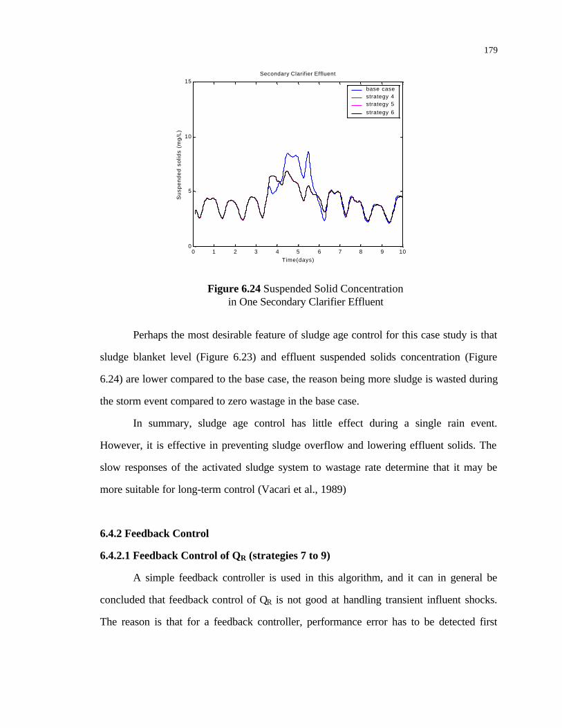
179
0 1 2 3 4 5 6 7 8 9 100
5
10
15
Time(days)
Su
spe
nd
ed
so
lids
(mg
/L)
Secondary Clarifier Effluent
base case strategy 4strategy 5strategy 6
Figure 6.24 Suspended Solid Concentration in One Secondary Clarifier Effluent
Perhaps the most desirable feature of sludge age control for this case study is that
sludge blanket level (Figure 6.23) and effluent suspended solids concentration (Figure
6.24) are lower compared to the base case, the reason being more sludge is wasted during
the storm event compared to zero wastage in the base case.
In summary, sludge age control has little effect during a single rain event.
However, it is effective in preventing sludge overflow and lowering effluent solids. The
slow responses of the activated sludge system to wastage rate determine that it may be
more suitable for long-term control (Vacari et al., 1989)
6.4.2 Feedback Control
6.4.2.1 Feedback Control of QR (strategies 7 to 9)
A simple feedback controller is used in this algorithm, and it can in general be
concluded that feedback control of QR is not good at handling transient influent shocks.
The reason is that for a feedback controller, performance error has to be detected first

180
before control actions are implemented and such action is therefore applied too late to
improve the performance of the activated sludge process.
Under this algorithm both nitrification and the effluent ortho-phosphate-P
concentration are worse than for the base case, with some improvement in effluent SS
and TOC concentration. Since DO concentration in the inner channel increases (Figure
6.25), elevated carbonaceous substance removal becomes possible. However, the
elevated DO concentration in the inner channel is not sufficient to improve nitrification.
The biomass concentrations for all three strategies are significantly reduced during the
storm event although they recover thereafter (Figure 6.26). It seems that the feedback
controller for QR tries to improve the effluent water quality at the expense of process
stability. Therefore, feedback control of QR may not be a good control in the sense that
effluent performance might be deteriorated.
0 1 2 3 4 5 6 7 8 9 100
0.5
1
1.5
2
2.5
3
Time(days)
DO
Co
nce
ntr
ati
on
(m
g/L
)
Inner Channel
base case strategy 7strategy 8strategy 9
Figure 6.25 DO Concentration in the Inner Upper Channel

181
0 1 2 3 4 5 6 7 8 9 101000
1500
2000
2500
3000
3500
4000
4500
5000
5500
6000
Time(days)
ML
SS
Co
nce
ntr
ati
on
(m
g/L
)
Inner Channel
base case strategy 7strategy 8strategy 9
Figure 6.26 MLSS Concentration in Inner Upper Channel
6.4.2.2 Feedback Control of Sludge Wastage Rate (strategies 10 to 12)
Compared to feedback control of QR, feedback control of QW achieves slightly
better effluent performance in terms of maximum effluent water quality indicators and
average effluent mass loadings. However, if compared to sludge age control strategies,
feedback control of Qw achieves the same control effect (Table 6.1).
0 1 2 3 4 5 6 7 8 9 1050
100
150
200
250
300
350
400
450
500
550
Time(days)
PA
O C
on
cen
tra
tio
n (
mg
/L)
Outer Upper CSTR
base case strategy 10strategy 11strategy 12
Figure 6.27 Phosphorus-Accumulating Bacteria Concentration in Outer Upper Channel
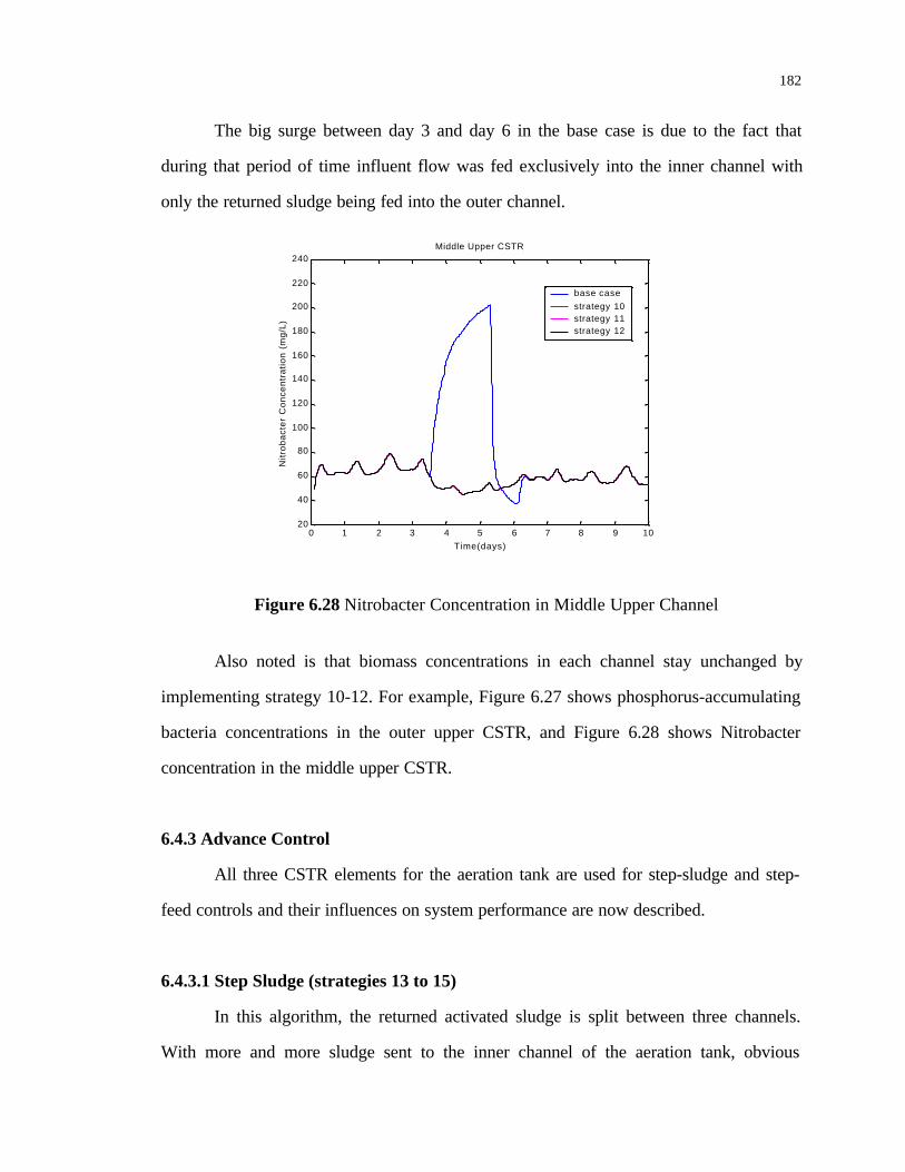
182
The big surge between day 3 and day 6 in the base case is due to the fact that
during that period of time influent flow was fed exclusively into the inner channel with
only the returned sludge being fed into the outer channel.
0 1 2 3 4 5 6 7 8 9 1020
40
60
80
100
120
140
160
180
200
220
240
Time(days)
Nitr
obac
ter
Con
cent
ratio
n (m
g/L)
Middle Upper CSTR
base case strategy 10strategy 11strategy 12
Figure 6.28 Nitrobacter Concentration in Middle Upper Channel
Also noted is that biomass concentrations in each channel stay unchanged by
implementing strategy 10-12. For example, Figure 6.27 shows phosphorus-accumulating
bacteria concentrations in the outer upper CSTR, and Figure 6.28 shows Nitrobacter
concentration in the middle upper CSTR.
6.4.3 Advance Control
All three CSTR elements for the aeration tank are used for step-sludge and step-
feed controls and their influences on system performance are now described.
6.4.3.1 Step Sludge (strategies 13 to 15)
In this algorithm, the returned activated sludge is split between three channels.
With more and more sludge sent to the inner channel of the aeration tank, obvious
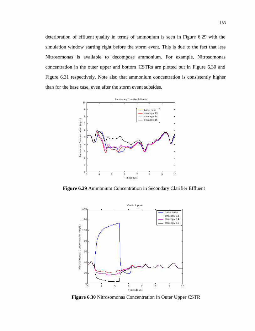
183
deterioration of effluent quality in terms of ammonium is seen in Figure 6.29 with the
simulation window starting right before the storm event. This is due to the fact that less
Nitrosomonas is available to decompose ammonium. For example, Nitrosomonas
concentration in the outer upper and bottom CSTRs are plotted out in Figure 6.30 and
Figure 6.31 respectively. Note also that ammonium concentration is consistently higher
than for the base case, even after the storm event subsides.
3 4 5 6 7 8 9 100
1
2
3
4
5
6
7
8
9
10
Time(days)
Am
mo
niu
m C
on
cen
tra
tio
n (
mg
/L)
Secondary Clarifier Effluent
base case strategy 13strategy 14strategy 15
Figure 6.29 Ammonium Concentration in Secondary Clarifier Effluent
3 4 5 6 7 8 9 100
20
40
60
80
100
120
140
Time(days)
Nit
roso
mo
na
s C
on
cen
tra
tio
n (
mg
/L)
Outer Upper
base case strategy 13strategy 14strategy 15
Figure 6.30 Nitrosomonas Concentration in Outer Upper CSTR
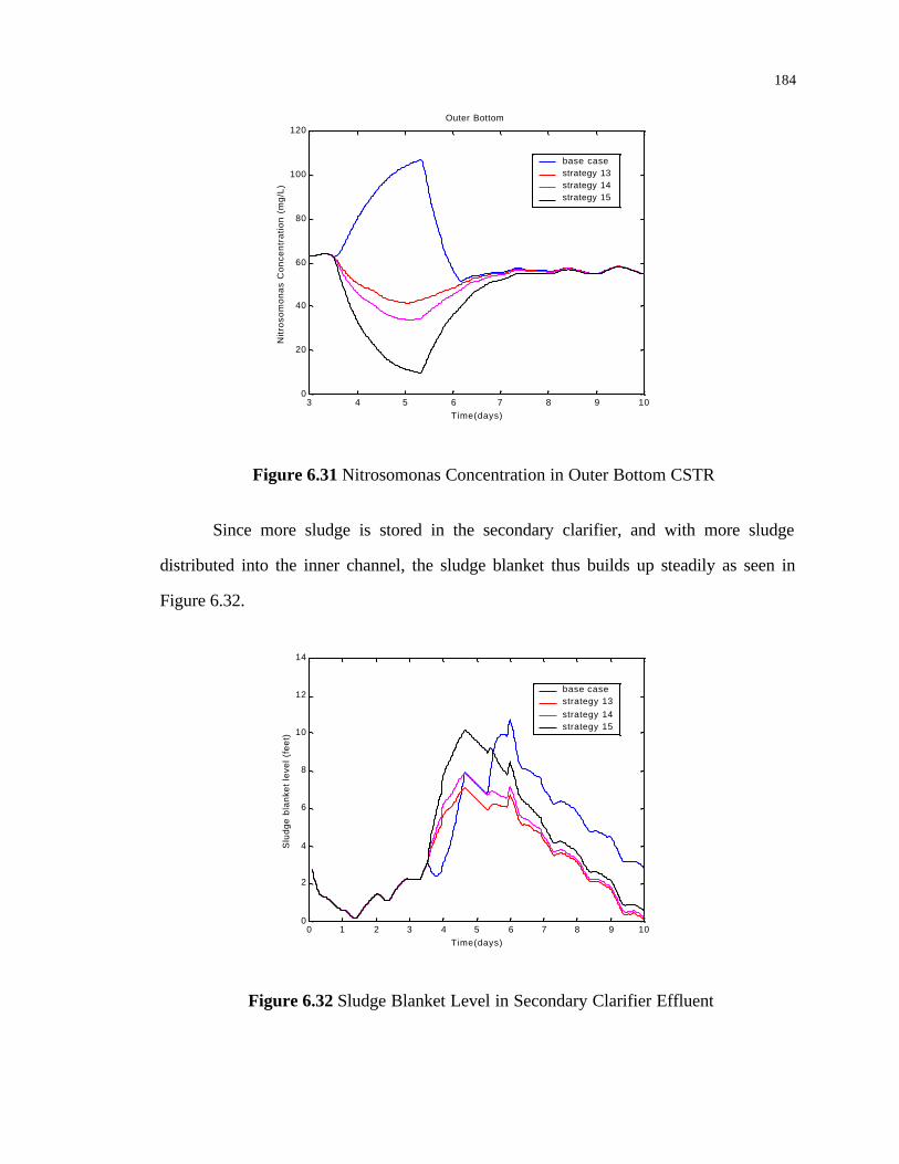
184
3 4 5 6 7 8 9 100
20
40
60
80
100
120
Time(days)
Nit
roso
mo
na
s C
on
cen
tra
tio
n (
mg
/L)
Outer Bottom
base case strategy 13strategy 14strategy 15
Figure 6.31 Nitrosomonas Concentration in Outer Bottom CSTR
Since more sludge is stored in the secondary clarifier, and with more sludge
distributed into the inner channel, the sludge blanket thus builds up steadily as seen in
Figure 6.32.
0 1 2 3 4 5 6 7 8 9 100
2
4
6
8
10
12
14
Time(days)
Slu
dge
blan
ket
leve
l (fe
et)
base case strategy 13strategy 14strategy 15
Figure 6.32 Sludge Blanket Level in Secondary Clarifier Effluent

185
In summary, step-sludge control can easily lead to sludge buildup if more sludge
is distributed closer to the outlet of the aeration tank, so that it is not good for storm event
control. So the closer returned sludge is kept to the head of aeration tank during the storm
event, the better it is for the system performance. Step-sludge control is advantageous
when the system is oxygen-limited at the inlet stage.
6.4.3.2 Step Feed (strategies 16 to 19)
As far as maximum effluent quality is concerned, step-feed configurations
(strategies 16 to strategy 18) achieve worse effluent ammonium, nitrite and ortho-
phosphate-P concentrations relative to the base case even thought none of them exceed
effluent standards. Figure 6.33 shows ortho-phosphate-P concentration in the secondary
clarifier effluent. The maximum ortho-phosphate-P concentration found during the storm
event is higher for strategies 16 to 18 than for the base case. The reason is that in the base
case only half of the influent was routed through the aeration tank No.2.
0 1 2 3 4 5 6 7 8 9 100
0.1
0.2
0.3
0.4
0.5
0.6
0.7
0.8
Time(days)
Ort
ho
-ph
osp
ha
te-p
Co
nce
ntr
atio
n (
mg
/L)
Secondary Clarifier Effluent
base case strategy 16strategy 17strategy 18
Figure 6.33 Ortho-Phosphate-P Concentration in Secondary Clarifier Effluent as a Result of Step Feed Control

186
In consideration that in case there is no tank for temporary storage of storm flow
during the storm event, one more simulation is then run to find out the maximum water
quality if all influent flow is put into the inner channel without diversion (strategy 19 in
Table 6.1). The results show that step-feed control evidently improves the effluent water
quality compared to strategy 19.
An attractive feature of step-feed control is that the sludge blanket level is
properly kept at a safe level such that sludge overflow would not take place. Such
behavior is highly desirable since it gives the system a better ability to withstand the
effects of more intense and frequent storm events. Figure 6.34 shows the behavior of the
sludge blanket level with step-feed control.
0 1 2 3 4 5 6 7 8 9 100
2
4
6
8
10
12
14
Time(days)
Slu
dge
blan
ket
leve
l (fe
et)
base case strategy 16strategy 17strategy 18
Figure 6.34 Sludge Blanket Level in Secondary Clarifier As A Result of Step Feed Control

187
0 1 2 3 4 5 6 7 8 9 100
1
2
3
4
5
6
7
Time(days)
Ort
ho
-ph
osp
ha
te-P
Co
nce
ntr
atio
n (
mg
/L)
crude sewage outer channel
Figure 6.35 Ortho-phosphate-P Concentration in the Crude Sewage and Outer Channel (Base Case)
DO concentration goes up towards the end of the bioreactor during a major storm
and ortho-phosphate-P is released upstream where the MLSS is being stored as a
consequence of the step-feed strategy being practiced at the Athens Wastewater
Treatment Facility No.2 as seen in Figure 6.35, where the curve in red is for the base
case. Obviously, ortho-phosphate-P concentration is higher in the outer channel than in
the crude sewage during the storm event, which is presumed to result from the effect of
ortho-phosphate-P release. This is certainly an operational complication of an otherwise a
promising strategy. However, this complication might be attenuated by keeping
sufficiently high DO concentration upstream during the storm events.
To summarize, step-feed manipulation is a promising strategy for storm event
control due to the fact that it not only improves effluent performance (even though only
effluent ortho-phosphate-P was shown in Figure 6.33), but also controls sludge blanket
level at a safe level.

188
6.4.4 DO Set-Point Control
For the base case the numbers of operating aerator units in the outer, middle, and
inner channel during the rain event are 10, 2, and 2 respectively. Figures 6.36-6.38 show
the number of operating aerator units needed in the outer, middle, and inner channel
respectively under various control strategies.
Figure 6.36 Number of Aerators in Outer Channel Under DO Set-point Control
Figure 6.37 Number of Aerators in Middle Channel Under DO Set-point Control
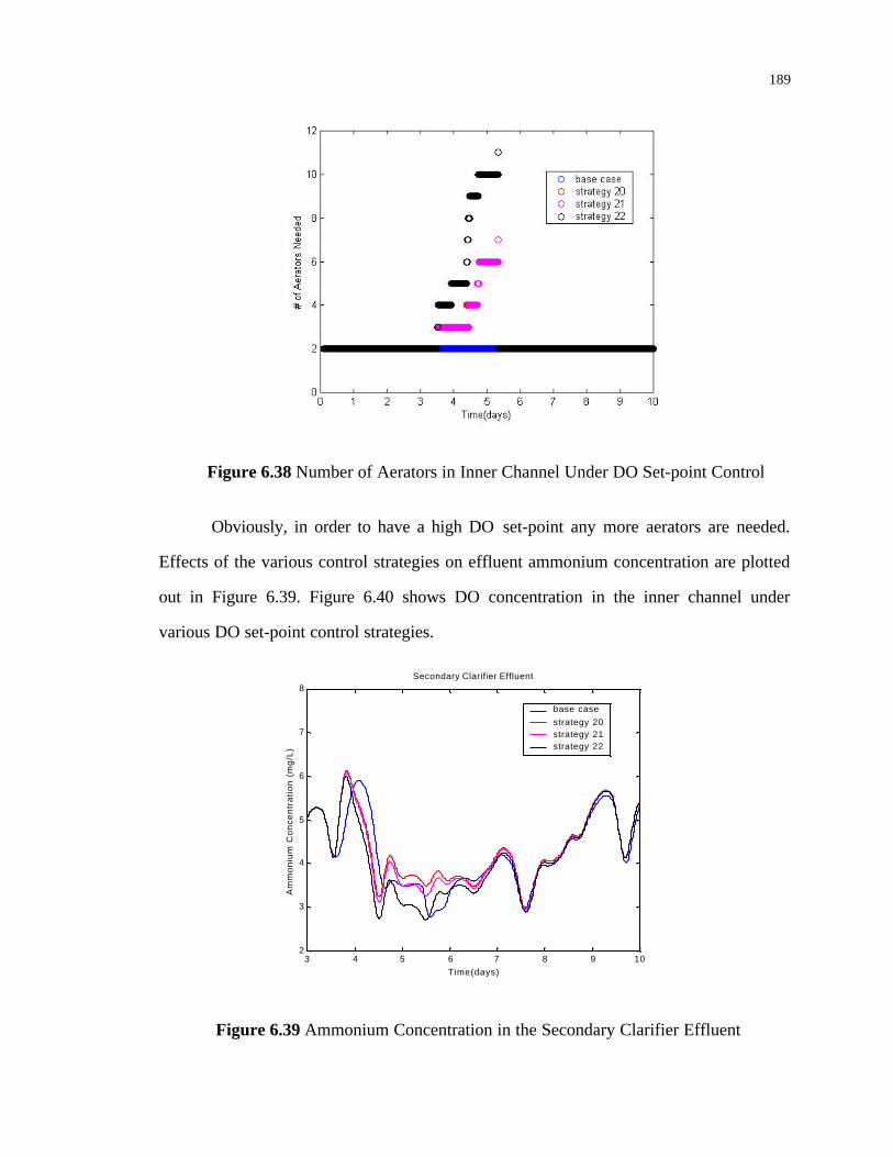
189
Figure 6.38 Number of Aerators in Inner Channel Under DO Set-point Control
Obviously, in order to have a high DO set-point any more aerators are needed.
Effects of the various control strategies on effluent ammonium concentration are plotted
out in Figure 6.39. Figure 6.40 shows DO concentration in the inner channel under
various DO set-point control strategies.
3 4 5 6 7 8 9 102
3
4
5
6
7
8
Time(days)
Am
mo
niu
m C
on
cen
tra
tio
n (
mg
/L)
Secondary Clarifier Effluent
base case strategy 20strategy 21strategy 22
Figure 6.39 Ammonium Concentration in the Secondary Clarifier Effluent

190
0 1 2 3 4 5 6 7 8 9 100
1
2
3
4
5
6
Time(days)
DO
Con
cent
ratio
n (m
g/L)
Inner Channel
base case strategy 20strategy 21strategy 22
Figure 6.40 DO Concentration in the Inner Channel
By running more aerators during the storm event, effluent quality, for instance,
ammonium can be improved to a certain extent, but obviously not significantly better
than for the base case (Figure 6.39). But these many aerators needed do not actually exist
in the treatment plant itself. Therefore, DO set-point control has to be balanced between
effluent quality and economic expenditures.
Table 6.1 Assessment of Operational Control Strategies of Activated Sludge Process During Storm Event
Maximum Concentration During the Storm Event (mg/L)No. ofStrategy ammonium nitrite nitrate TOC ortho-phosphate-P sseffluent
standard 17.0 0.2 2.5 30.0 2.0 30.0
0 5.91E+0 1.10E-1 3.01E+0 1.64E+1 3.51E-1 8.52E+01 6.14E+0 1.22E-1 3.02E+0 1.02E+1 3.81E-1 6.55E+02 6.00E+0 1.21E-1 3.02E+0 8.76E+0 3.79E-1 8.73E+03 5.95E+0 1.23E-1 3.02E+0 8.12E+0 3.79E-1 1.04E+14 6.05E+0 1.21E-1 3.02E+0 9.84E+0 3.79E-1 6.94E+05 6.06E+0 1.21E-1 3.02E+0 9.84E+0 3.79E-1 6.94E+06 6.06E+0 1.21E-1 3.02E+0 9.84E+0 3.79E-1 6.94E+07 6.07E+0 1.21E-1 3.02E+0 9.14E+0 3.79E-1 7.53E+08 6.07E+0 1.21E-1 3.02E+0 9.97E+0 3.79E-1 6.82E+09 6.07E+0 1.21E-1 3.02E+0 9.79E+0 3.79E-1 6.95E+0

191
10 6.07E+0 1.21E-1 3.02E+0 9.84E+0 3.79E-1 6.94E+011 6.07E+0 1.21E-1 3.02E+0 9.84E+0 3.79E-1 6.94E+012 6.07E+0 1.21E-1 3.02E+0 9.84E+0 3.79E-1 6.94E+013 5.78E+0 1.50E-1 3.02E+0 9.78E+0 3.79E-1 7.02E+014 5.83E+0 1.53E-1 3.02E+0 1.06E+1 3.79E-1 7.12E+015 5.98E+00 1.61E-1 3.02E+0 1.38E+1 3.78E-1 7.66E+016 6.07E+0 1.21E-1 3.02E+0 9.84E+0 3.79E-1 6.94E+017 6.25E+0 1.13E-1 3.02E+0 1.06E+1 3.75E-1 6.80E+018 6.73E+0 1.11E-1 3.01E+0 1.67E+1 3.69E-1 6.26E+019 7.38E+0 1.10E-1 3.01E+0 2.41E+1 3.64E-1 5.29E+020 6.13E+0 1.18E-1 3.02E+0 1.05E+1 3.79E-1 6.94E+021 6.11E+0 1.20E-1 3.02E+0 1.01E+1 3.79E-1 6.94E+022 6.01E+0 1.33E-1 3.02E+0 9.30E+0 3.79E-1 6.94E+0
Average Effluent Loadings (Kg/h)No. ofStrategy ammonium nitrite nitrate TOC ortho-phosphate-P ss
0 1.40E+0 2.89E-2 7.91E-1 2.22E+00 8.87E-2 2.16E+01 1.35E+0 3.46E-2 6.53E-1 1.21E+0 7.99E-2 1.82E+02 1.29E+0 3.49E-2 7.08E-1 1.06E+0 8.12E-2 2.30E+03 1.27E+0 3.47E-2 7.36E-1 9.90E-1 8.24E-2 2.63E+04 1.31E+0 3.41E-2 6.58E-1 1.15E+0 7.88E-2 1.87E+05 1.32E+0 3.42E-2 6.61E-1 1.15E+0 7.92E-2 1.88E+06 1.33E+0 3.45E-2 6.68E-1 1.16E+0 8.00E-2 1.90E+07 1.31E+0 3.49E-2 6.91E-1 1.10E+0 8.07E-2 2.04E+08 1.34E+0 3.46E-2 6.66E-1 1.18E+0 8.02E-2 1.89E+09 1.33E+0 3.47E-2 6.71E-1 1.16E+0 8.03E-2 1.92E+010 1.32E+0 3.44E-2 6.65E-1 1.16E+0 7.96E-2 1.89E+011 1.30E+0 3.38E-2 6.54E-1 1.13E+0 7.84E-2 1.85E+012 1.32E+0 3.43E-2 6.64E-1 1.15E+0 7.96E-2 1.89E+013 1.28E+0 4.02E-2 7.03E-1 1.15E+0 8.04E-2 1.93E+014 1.36E+0 4.31E-2 6.57E-1 1.27E+0 8.08E-2 1.96E+015 1.61E+0 4.39E-2 5.59E-1 1.84E+0 8.22E-2 2.07E+016 1.33E+0 3.47E-2 6.71E-1 1.17E+0 8.03E-2 1.90E+017 1.30E+0 2.94E-2 7.19E-1 1.39E+0 7.96E-2 1.85E+018 1.43E+0 2.49E-2 7.11E-1 2.24E+0 7.86E-2 1.70E+019 1.72E+0 2.28E-2 5.72E-1 3.27E+0 7.70E-2 1.40E+020 1.41E+0 3.23E-2 6.22E-1 1.25E+0 8.04E-2 1.90E+021 1.38E+0 3.42E-2 6.41E-1 1.21E+0 8.03E-2 1.90E+022 1.28E+0 3.86E-2 7.04E-1 1.11E+0 8.02E-2 1.90E+0
6.4.5 Evaluation of Control Strategies (Strategy 1-Strategy 22)
All of the 22 control strategies have thus been tested. We are now in a position to
compare them and pick out the best and worst among them, excluding strategy 19, which
is an extreme case and is introduced to support the discussion of Section 6.4.3.2. Table
6.2 lists the best and worst strategies as far as maximum nutrient concentrations in the

192
secondary clarifier are concerned. Table 6.3 lists the best and the worst strategy as far as
average effluent loadings are concerned.
Table 6.2 Comparison of Control Strategies Based on Maximum Nutrient Concentration in the Secondary Clarifier Effluent
ammonium nitrite nitrate TOC ortho-phosphate-P
ss
best strategy(No.)
No.13 No.18 No.3 No.18 No.18
worst strategy(No.)
No.18 No.15 No.18 No.1 No.3
differencerelative to basecase for worststrategy (%)
14% 46% 2% 9% 22%
over effluentstandards forworst strategy?
No No No No No
Table 6.3 Comparison of Control Strategies Based on Average Effluent Loadings in the Secondary Clarifier Effluent
ammonium nitrite nitrate TOC ortho-phosphate-P
ss
best strategy(No.)
No.3 No.18 No.18 No.3 No.18 No.18
worst strategy(No.)
No.18 No.15 No.3 No.18 No.3 No.3
differencerelative to basebase for worststrategy (%)
2% 52% 7% 1% 7% 22%
As far as maximum effluent ammonium concentration is concerned (Table 6.2),
strategy 18 (step-feed control) is ranked the worst (6.8 mg/L) because it is 14% higher
than that in the base case (6.0mg/L). However, the effluent standard for ammonium is 17
mg/L. So even in the worst case, effluent ammonium concentration is not even half-way
close to the effluent standard. As far as average effluent loadings are concerned (Table
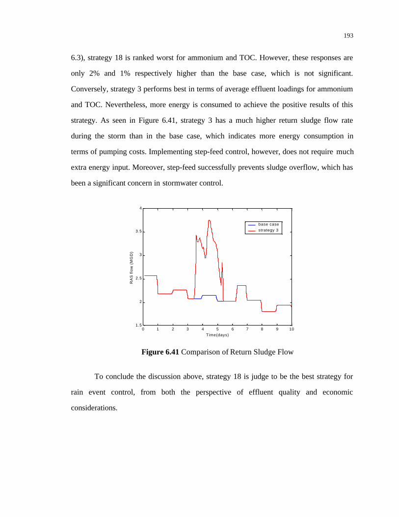
193
6.3), strategy 18 is ranked worst for ammonium and TOC. However, these responses are
only 2% and 1% respectively higher than the base case, which is not significant.
Conversely, strategy 3 performs best in terms of average effluent loadings for ammonium
and TOC. Nevertheless, more energy is consumed to achieve the positive results of this
strategy. As seen in Figure 6.41, strategy 3 has a much higher return sludge flow rate
during the storm than in the base case, which indicates more energy consumption in
terms of pumping costs. Implementing step-feed control, however, does not require much
extra energy input. Moreover, step-feed successfully prevents sludge overflow, which has
been a significant concern in stormwater control.
0 1 2 3 4 5 6 7 8 9 101.5
2
2.5
3
3.5
4
Time(days)
RA
S f
low
(M
GD
)
base case strategy 3
Figure 6.41 Comparison of Return Sludge Flow
To conclude the discussion above, strategy 18 is judge to be the best strategy for
rain event control, from both the perspective of effluent quality and economic
considerations.

194
6.5 FURTHER CONSIDERATIONS
6.5.1 Effect of Alternative Effective Mixing Volume
In this section, more simulations will be run based on the best strategy (strategy
18 in Table 6.1) to explore the impact of alternative equally effective mixing volumes in
each channel (from 50% effective mixing to approaching 100% effective mixing) on the
system performance. The following three options will be tested (Table 6.4). The relevant
statistics are computed in Table 6.5. In Table 6.5 ‘case 0’ refers to the base case.
Table 6.4 Test Cases for Impact of Alternative Effective Mixing Volumes
Outer Channel Middle Channel Inner ChannelEffectiveMixing
(%)
Non-EffectiveMixing
(%)
EffectiveMixing
(%)
Non-EffectiveMixing
(%)
EffectiveMixing
(%)
Non-EffectiveMixing
(%)Case 1 50 50 50 50 50 50Case 2 80 20 80 20 80 20Case 3 95 5 95 5 95 5
Evidently by having ever larger effective mixing volumes in each channel,
effluent water quality in terms of ammonium is significantly improved, and significantly
better than strategy 18 in Table 6.1. To accompany this argument, Figure 6.42 shows
ammonium concentration in the outer channel; Figure 6.43 is the DO concentration at the
same location; and Figure 6.44 gives the corresponding Nitrosomonas concentration.
Effluent water quality in terms of other nutrient concentrations is improved as well,
except for nitrate. The reason might be due to the fact that elevated DO concentrations
result in more nitrite being transformed to nitrate.

195
0 1 2 3 4 5 6 7 8 9 100
1
2
3
4
5
6
7
8
Time(days)
Am
mo
niu
m C
on
cen
tra
tio
n (
mg
/L)
Secondary Clarifier Effluent
base casecase 1 case 2 case 3
Figure 6.42 Ammonium Concentration in the Outer Channel
0 1 2 3 4 5 6 7 8 9 100
1
2
3
4
5
6
7
8
9
10
Time(days)
DO
Con
cent
ratio
n (m
g/L)
Outer Channel
base casecase 1 case 2 case 3
Figure 6.43 DO Concentration in the Outer Channel

196
0 1 2 3 4 5 6 7 8 9 1010
20
30
40
50
60
70
80
90
100
110
120
Time(days)
Nit
roso
mo
na
s C
on
cen
tra
tio
n (
mg
/L)
Outer Channel
base casecase 1 case 2 case 3
Figure 6.44 Nitrosomonas Concentration in the Outer Channel
6.5.2 Effect of One Layer Model Structure
Further to cases 1-3, one more simulation will be run here to test out the best
strategy (strategy 18 in Table 6.1) with no flow routed through the base of the channel
(the lower set of three CSTRs), i.e., with all of the volume of the actual tank assigned to
the upper CSTRs. The statistics of the model results are listed in Table 6.5 as case 4.
Clearly, effluent water quality in terms of ammonium is further improved to a small
extent, but the system performance in terms of nitrite and nitrate has deteriorated
compared to case 3.
In order to achieve good nitrification in the case study plant, large effective
mixing volume proves to be an extremely important issue. The revised two-layer model
makes evaluation of system performance under better effective mixing volume possible.
Some form of deliberate mixing control might cure this plant’s inability to achieve good
nitrification, such as using diffused air at the bottom of the tank to increase effective
mixing volume and resuspension. Maier and Krauth (1998) reported that surface aeration
systems did not nitrify as well as diffused systems due to DO shortage. Unfortunately,

197
this option cannot be tested out in the current model structure, because it is assumed in
the model that the bottom layers are anoxic. If oxygen input is exerted into the bottom
CSTRs, they become oxic and therefore the biochemical mechanisms in the bottom
layers need to be changed completely accordingly.
Table 6.5 Assessment of Further Test Cases
Maximum Concentration During the Storm Event (mg/L)No. ofCase ammonium Nitrite nitrate TOC ortho-phosphate-P ss
effluentstandard 17.0 0.2 2.5 30.0 2.0 30.0
0 5.91E+0 1.10E-1 3.01E+0 1.64E+1 3.51E-1 8.52E+01 4.84E+0 8.15E-2 4.82E+0 1.52E+1 3.57E-1 6.30E+02 3.91E+0 8.37E-2 6.25E+0 1.39E+1 3.47E-1 6.33E+03 3.67E+0 8.57E-2 6.59E+0 1.35E+1 3.44E-1 6.35E+04 3.60E+0 8.68E-2 6.69E+0 1.35E+1 3.43E-1 6.35E+0
Average Effluent Loadings (Kg/h)No.of
Caseammonium nitrite nitrate TOC Ortho-phosphate-P ss
0 1.40E+0 2.89E-02 7.91E-01 2.22E+00 8.87E-2 2.16E+01 1.09E+0 2.33E-2 9.62E-1 2.00E+0 7.89E-2 1.69E+02 8.73E-1 2.30E-2 1.22E+0 1.78E+0 7.98E-2 1.67E+03 8.21E-1 2.31E-2 1.31E+0 1.72E+0 8.00E-2 1.66E+04 8.07E-1 2.33E-2 1.34E+0 1.71E+0 8.00E-2 1.66E+0
6.6 CONCLUSIONS
The results of a detailed assessment of control strategies for the activated sludge
process have been presented in this Chapter. The controlled event is a short-term event
with storm runoff as the chosen example. The following conclusions can be drawn from
these results:
q Of the tested strategies, the advanced controllers are found to be more powerful than
the “conventional” and “feedback” ones for controlling the deleterious effects of the
rain events;
q Of the tested control variables, step-feed can be declared to be the best for rain-event
control;

198
q Great effective mixing volume is essential for good nitrification.

199
CHAPTER 7
CONCLUSIONS AND RECOMMENDATIONS
7.1 INTRODUCTION
This very last chapter is comprised of two parts. Firstly, the conclusions from
major sections of the dissertation are presented. Secondly, recommendations for future
work are presented.
7.2 CONCLUSIONS
Throughout the program of research presented attempts have been made to
address the problems of modeling and operational control of the activated sludge process.
The following is concluded from the results of the study:
q The scope and quality of the some 60-day data acquired from the Athens Wastewater
Treatment Facility No.2 with the EPCL are found to be exceptional, compared to
what has been reported in the literature, and thus provides a solid base for subsequent
model and control strategy development;
q A dynamic multiple species model has been developed for simulating nitrogen,
carbon, and ortho-phosphate-P removal in the activated sludge system. Significant
contributions have been made in the characterization of solute and particulate
transport in the activated sludge process, and simultaneous nitrification and
denitrification in the aerated zones;

200
q The constituent hypotheses of the proposed model have first been tested against a 19-
day period data from the experiment at the treatment plant. The general conclusion of
this assessment is that the model, as a whole, is acceptable for simulating the behavior
of the activated sludge process. From sensitivity analyses of the model parameters,
especially those associated with the hydraulic transport component, it is found that
the chosen values for these parameters are appropriate;
q Following this preliminary assessment of its structure, the model has been validated
against another set of data, covering some 18 days. Evaluation results demonstrate the
model’s capacity to simulate the system performance, particularly under extreme flow
conditions;
q Using the model thus identified, a detailed analysis of control strategies for regulating
the effects of storm events has been undertaken. In general, it is found that,
• Of the tested strategies, the advanced controllers are found to be more powerful
than the “conventional” and “feedback” ones for the rain events;
• Of the tested control variables, step-feed can be declared to be the best for rain
event control;
• An effective mixing volume is essential to good nitrification.
7.3 RECOMMENDATIONS FOR FUTURE WORK
Based on the results of this study, the following recommendations for future work are
made:
q From the perspective of data collection, detailed information on aerator operation and
sludge wastage processing should be recorded for more accurate model results;

201
q A tracer study should be undertaken to confirm the current 2-layer model
configuration of the aeration tank;
q Detailed and sophisticated analyses based on the Kalman filtering-smoothing
algorithms would also be helpful to confirm that it is essential to reconstruct the
model into a 2-layer configuration. Using the signal extraction algorithms to separate
trend and noise components from a periodic component, incisive insights into the two
fundamental aspects of bioreactor reactor behavior, its mixing and biomass activities,
together with their variation with time, could thereby be exposed;
q Improvement of the proposed model in terms of biological removal of ortho-
phosphate-P is very desirable with increasing knowledge of this process in the future;
q For the proposed dynamic model, further refinement of the clarification and
thickening sub-models is essential if any improvement in simulation performance is
required. More detailed exploration of biochemical reactions during clarification,
thickening and sludge recycle, will be desirable.
q There is scope for the wider application of formal search techniques for model
parameter estimation, including in particular the increasing popular methods of
controlled random search.

202
REFERENCES
Abasaeed, A. E. (1997). “Sensitivity Analysis on a Sequencing Batch Reactor Model I.
Effect of Kinetic Parameters”. Journal of Chemical Technology in Biotechnology,
70, 379-383.
Abeling, U., and Seyfried, C. F. (1992).“Anaerobic-Aerobic Treatment of High-Strength
Ammonium Wastewater Nitrogen Removal via Nitrite”. Water Science and
Technology, 26, 5-6, 1007-1015.
Akunna, J. C., Biazeau, C., and Moletta, R. (1993).“Nitrate and Nitrite Reductions with
Anaerobic Sludge Using Various Sources: Glucose, Glycerol, Acetic Acid, Lactic
Acid and Methanol”. Water Research, 27, 8,1303-1312.
Alex, J., Tschepetzki, R., Jumar, U., and Rosenwinkel, K. (1998).“Analysis and Design
of Suitable Model Structures for Activated Sludge Tanks with Circulating Flow”.
Proceeding of Aquatech’98 on Application of Models in Water Management,
Amsterdam, The Netherlands, September 24-25.
Alleman, J. E. (1984).“Elevated Nitrite Occurrence in Biological Wastewater Treatment
Systems”. Water Science and Technology, 17, 2-3, 409-419.
Allison, C., and MacFarlane, G. T. (1989).“Dissimilatory Nitrate Reduction by
Propionibacterium Acnes”. Applied and Environmental Microbiology, 55, 11,
2899-2903.

203
Andreottola, G., Bortone, G., and Tilche, A. (1997).“Experimental Validation of a
Simulation and Design Model for Nitrogen Removal in Sequencing Batch
Reactors”. Water Science and Technology, 35, 1,113-120.
Andrews, J. F. (1974).“Review Paper: Dynamic Models and Control Strategies for
Wastewater Treatment Process”. Water Research, 8, 1, 261-289.
Ante, A., Besche, H. U., and Voss, H. (1994). “A Mathematical Model for Enhanced
Biological Phosphorus Removal”. Water Science and Technology, 30,2,193-203.
Antoniou, P., Koopman, B., Jain, R., Holloway, B., Lyberatos, G., and Svoronos, S. A.
(1990).“Effect of Temperature and pH on the Effective Maximum Specific
Growth Rate of Nitrifying Bacteria”. Water Research, 24,1,97-101.
Applegate, C.S., Wilder, B., and DeShaw, J.R. (1980). “Total Nitrogen Removal in a
Multi-Channel Oxidation System”. Journal-Water Pollution Control Federation,
52, 568-577.
Arun, V., Mino, T., and Matsuo, T. (1987).“Biological Mechanisms of Acetate Uptake
Mediated by Carbonhydrate Consumption in Excess Phosphate Removal
Systems”. Water Research, 22, 5, 565-570.
Arun, V., and Lohani, B. N. (1988). “Estimating Supernatant Recycle from Sludge
Treatment”. Journal of Environment Engineering, 114, 2, 447-453.

204
Balmelle, Bnguyen, K. M., Capdeville, B., Cornie, J. C., and Deguin, A. (1992).“Study of
Factors Controlling Nitrite Build-up in Biological Processes for Water
Nitrification”. Water Science and Technology, 26, 5-6, 1017-1025.
Barker, P. S., and Dold, P. L. (1996).“Denitrification Behavior in Biological Excess
Phosphorus Removal Activated Sludge Systems”. Water Research, 30, 4,769-780.
Barker, P.S., and Dold, P. L. (1997a).“General Model for Biological Nutrient Removal
Activated-Sludge Systems: Model Presentation”. Water Environment Research,
69, 7-8, 969-984.
Barker, P. S., and Dold, P. L. (1997b).“General Model for Biological Nutrient Removal
Activated-Sludge Systems: Model Application”. Water Environment Research,
69, 7-8, 985-991.
Barnard, J. L. (1982).“The Influence of Nitrogen on Phosphorus Removal in Activated
Sludge Plants”. Water Science and Technology, 14, 1/2, 31-45.
Barnard, J. L. (1983). “Background to Biological Phosphorus Removal”. Water Science
and Technology, 15,1-13.
Beck, M. B. (1981).“Operational Estimation and Prediction of Nitrification Dynamics in
the Activated Sludge Process”. Water Research, 15, 7-12, 1313-1330.
Beck, M. B. (1984). “Modeling and Control Studies of the Activated Sludge Process at
Norwich Sewage Works”. Trans. Inst. M. C., 6, 3, 117-131.

205
Beck, M. B. (1986).“Identification, Estimation and Control of Biological Wastewater
Treatment Process”, IEE Proceedings, 133, 5, 254-264.
Beck, M. B. (1987). “Water Quality Modeling: A Review of the Analysis of
Uncertainty”. Water Resources Research, 23, 8, 1393-1442.
Beck, M. B., and Liu, R. (1998).“On-line Analyzers and Modeling in Wastewater
treatment Plant Control”. Preprint, Pre-Conference Workshop on Online
Analyzers Based Control of Wastewater Treatment Plants, Water Environment
Federation, 71st Annual Conference and Exposition, Orlando, Florida, (1998),
11p.
Beck, M. B., and Liu, R. (1999).“Data Processing and Interpretation: Filtering,
Smoothing, and Signal Extraction”. Preprint, Pre-Conference Workshop
Automatic Monitoring and Control of Wastewater Treatment Plants, Water
Environment Federation, 72nd Annual Conference and Exposition, New Orleans,
Louisiana, (1999), 7p.
Benefield, L. D., and Randall, C. W. (1980). Biological Process Design for Wastewater
Treatment. Prentice Hall Inc., New Jersey.
Bertanza, G. (1997).“Simultaneous Nitrification-Denitrification Process in Extended
Aeration Plants: Pilot and Real Scale Experiences”. Water Science and
Technology, 35, 6,53-61.
Bliss, P. J., and Barnes, D. (1986).“Modeling Nitrification in Plant Scale Activated
Sludge”. Water Science and Technology, 18, 6,139-148.

206
Bogdan, L., Lomotowski, J., Nahorski, Z., Studzinski, J., and Szetela, R. (1998).
“Mathematical Model and Its Calibration for Rzeszow Wastewater Treatment
Plant”. Environment Protection Engineering, 24,1-2,95-112.
Bradstreet, K. A., and Johnson, G. R. (1994).“Study of Critical Operational Parameters
for Biological Nitrogen Reduction at a Municipal Wastewater Treatment Plant”.
Proceeding of the 67th Annual Conference of Water Environment Federation,
Chicago, I11, 1,669.
Brdjanovic, D., van Loosdrecht, M. C. M., Hooijmans, C. M., Alaerts, G. L. J., and
Heijnen, J. J. (1997). “Temperature Effects on Physiology of Biological
Phosphorus Removal”. Journal of Environmental Engineering,123, 2,144-153.
Brewer,H., Stephenson,J.P., and Green,D. (1995). “Plant Optimization Using Online
Phosphorus Analyzers and Automated SRT Control to Achieve Harbour
Selisting”. Proceedings of Water Environment Federation 68th Annual Conference
and Exposition, Miami Beach, Florida, 5, 673.
Brune, D. (1985). “Optimal Control of the Complete-Mix Activated Sludge Process”.
Environmental Technology Letters ETLEDB, 6, 11, 467-476.
Buhr, H. O. (1984).“Making Full Use of Step Feed Capability”. Journal-Water Pollution
Control Federation, 56, 4, 325-332.
Burrows, L. J., Stokes, A. J., West, J. R., Foster, C. F., and Martin, A. D.
(1999).”Evaluation of Different Analytical Methods for Tracer Studies in
Aeration Lanes of Activated Sludge Plants”. Water Research, 33,2,367-374.

207
Buswell, A. M., Shiota, T., Lawrence, N., and Meter, I. V. (1954).“Laboratory Studies on
the Kinetics of the Growth of Nitrosomonas with Relation to the Nitrification
Phase of the BOD Test”. Applied Microbiology, 2, 21-25.
Capital Controls (Minworth Systems Limited) (1994). “MSL‘FT For Windows User’s
Manual”, UK.
Capital Controls (Minworth Systems Limited) (1996). “GFX for Windows User’s
Manual”, Version 2.51d, UK.
Capital Controls (Minworth Systems Limited) (1996). “’Translate’ For Windows User’s
Manual”, UK.
Capital Controls (Minworth Systems Limited) (1996). “FT For Windows User’s
Manual”, UK.
Capital Controls (Minworth Systems Limited) (1997). “Respirometer Manual”, Version
4.1, UK.
Capital Controls (Minworth Systems Limited) (1997). “Ammonia Monitor User Manual
(version 4.1)”, UK.
Capodaglio, A. G. (1994).“Evaluation of Modeling Techniques for Wastewater
Treatment Plant Automation”. Water Science and Technology, 30,2,149-156.

208
Carlsson, H., Aspegren, H., and Hilmer, A. (1996). “Interactions Between Wastewater
Quality and Phosphorus Release in the Anaerobic Reactor of the EBPR Process”.
Water Research, 30, 6, 1517-1527.
Carter, K. B. (1985).“Contract Operations: Private Contracts for Public Work”. Journal-
Water Pollution Control Federation, 57,7,750-755.
Carucci, A., Rolle, E., and Smurra, P. (1999).“Management Optimization of a Large
Wastewater Treatment Plant”. Water Science and Technology, 39,4,129-136.
Casey, T. G., Wentzel, M. C., Ekama, G. A., Lowenthal, R. E., and Marais, G. v. R.
(1994). “A Hypo-thesis for the Causes and Control of Anoxic-Aerobic (AA)
Filament Bulking in Nutrient Removal Activated Sludge Systems”. Water Science
and Technology, 29,7,203-210.
Chen, J. N. (1993). “Modeling and Control of the Activated Sludge Process: Towards a
Systematic Framework”. Ph.D Thesis, Imperial College.
Choi, E., Rhu, D., Yun, Z., and Lee, E. (1998).“Temperature Effects on Biological
Nutrient Removal System with Weak Municipal Wastewater”. Water Science and
Technology, 37, 9,219-226.
Choi, S. H., Colin, F., Sardin, M., and Prost, C. (1993).“Settling Velocity Model of
Activated Sludge”. Water Research, 27,7,1237-1242.
Cinar, O., Daigger, G. T., and Graef, S. P. (1996).“Evaluation of IAWQ Activated Sludge
Model No.2 Using Four full-scale Wastewater Treatment Plants”. Proceeding of

209
the 69th Annual Technical Conference and Exposition of Water Environment
Federation, Dallas, Texas.
Cinar, O., Daigger, C. F., Yuang, H. C., and You, S. J. (1998).“Evaluation of IAWQ
Activated Sludge Model No.2 Using Steady State Data from Four Full-Scale
Wastewater Treatment Plants”. Water Environment Research, 70,6,1216-1224.
Cliff, R. C., and Garrett, M. T. (1988). “Improved Oxygen Dissolution Control for
Oxygen Activated Sludge”. Water Science and Technology, 20, 4/5, 101-108.
Coen, F., Vanderhaegen, B., Boonen, I., Vanrolleghem, P. A., and Van Meenen, P.
(1997).“Improved Design and Control of Industrial and Municipal Nutrient
Removal Plants Using Dynamic Models”. Water Science and Technology, 35,10,
53-63.
Colby, S., and Ekster, A. (1997).“Control-Loop Fault Detection”. Water Environment
and Technology, 9,11,43-46.
Comeau, Y., Hall, K. J., Kancock, R. E. W., and Oldham, W. K. (1986).“Biochemical
Model for Enhanced Biological Phosphorus Removal”. Water Research, 20,12,
1511-1521.
Comeau, Y., Oldham, W. K., and Hall, K. J. (1987).“Dynamics of Carbon Reserves in
Biological Dephosphatation of Wastewater”. Pergamon Press, Oxford.

210
Cote, M., Grandjean, B. P. A., Lessard, P., and Thibault, J. (1995).”Dynamic Modeling
of the Activated Sludge Process: Improving Prediction Using Neural Networks”.
Water Research, 29,4,995-1004.
Culp, R. L., Wesner, G. M., and Culp, G. L. (1978). Handbook of Advanced Wastewater
Treatment. Van Nostrand Reinhold, New York.
Czeczot, J. (1998).“Model-Based Control of the Substrate Concentration in an Aeration
Basin Using the Wastewater Level”. Water Science and Technology, 37,12,335-
342.
Daigger,G.T., and Littleton, H.X. (2000). “Characterization of Simultaneous Nutrient
Removal in Staged, Closed-Loop Bioreactors”. Water Environment Research,
72,3,330-339.
Derco, J., Kralik, M., Hutnan, M., Bodik, I., and Cernak, R. (1994).”Modeling of the
Carrousel Plant”. Water Science and Technology, 30,6,345-354.
Dick, R. I. (1985). “Dynamic and Control of Solids-Liquid Separation in the Activated
Sludge Process”. Ph.D Dissertation, Rice University.
Dick, R.I., and Young, K.W. (1972). “Analysis of Thickening Performance of Final
Settling Tanks”. Proceedings of the 27th Industrial Waste Conference, Part 1, 33-
54. Purdue University,Lafayette, Indiana.
Diehl, S., and Jeppsson, U. (1998).“A Model for the Settler Coupled to the Biological
Reactor”. Water Research, 32,2,331-342.

211
Dochain, D., Agathos, S. N., and Vanrolleghem, P. (1997).“Asymptotic Observers as a
Tool for Modeling Process Dynamics”. Water Science and Technology, 36,5,259-
268.
Dold, P. L., and Marais, G.v.R. (1986). “Evaluation of the General Activated Sludge
Model Proposed by the IAWPRC Task Group”. Water Science and Technology,
18,63-69.
Downes, M. T. (1988).“Aquatic Nitrogen Transformations at Low Oxygen
Concentrations”. Applied and Environmental Microbiology, 54,1,172-175.
Drews, R. J. L. C., and Greef, A. M. (1973). “Nitrogen Elimination by Rapid Alternation
of Aerobic/Anoxic Conditions in Orbal Activated Sludge Plants”. Water
Research,7,1183-1194.
Ducato, R., and Galluzzo, M. (1995). “Dynamic Simulation of a NDBEPR Activated
Sludge Process”. Computers in Chemical Engineering, 19, supplement, 441-446.
Duchesne, S., Beck, M. B., and Reda, A. L. L. (2000). “Ranking Stormwater Control
Strategies Under Uncertainty: The River Cam Case Study”. 5th International
Symposium on Systems Analysis and Computing in Water Quality Management,
Ghent, Belgium, September 18-20, 2000. 6.17-6.24.
Dupont, R., and Dahl, C. (1995). “A One-dimensional Model for A Secondary Settling
Tank Including Density Current and Short-circuiting”. Water Science and
Technology, 31,2, 215-224.

212
Dupont, R. and Henze, M. (1992). “Modeling of the Secondary Clarifier Combined with
the Activated Sludge Model No.1”. Water Science and Technology, 25,6,285-
300.
Eckenfelder, W. W. et al. (1985). “The Activated Sludge Process: State of the Art”. CRC
Critical Reviews in Environ. Contr., 15, 2, 111-178.
Effler, S. W., and Hennigan, R. D. (1996). “Onondaga Lake, New York: Legacy of
Pollution”. Lake and Reservoir Management, 12, 1, 1-13.
Eliosov, B., Rubin, D., Libman, V., and Argaman, Y. (1997). “A New Approach to the
Effect of Dissolved Oxygen on the Rate of Denitrification”. Proceeding of the 70th
Annual Water Environment Federation Conference and Exposition, Chicago, I11,
1, 325.
Fuhs, G. W., and Chen, M. (1975).“Microbiological Basis of Phosphate Removal in the
Activated Sludge Process for the Treatment of Wastewater”. FEMS Microbiology
Ecology, 2,119-138.
Fujimoto, E., Iwahori, K., and Sato, N. (1981). “Automatic Measurement Device of the
Respiration Rate and Experimental Investigation on the Constant DO Control by
Using the Device for the Activated Sludge Process”. Water Science and
Technology, 13, 9, 193-198.
Fukase, T., Shibata, M., and Miyaji, Y. (1985). “Factors Affecting Biological Removal of
Phosphorus”. Water Science and Technology, 17,11/12, 187.

213
Funamizu, N., and Takakuwa, T. (1994).“Simulation of the Operating Conditions of the
Municipal Wastewater Treatment Plant at Low Temperature Using a Model that
includes the IAWPRC Activated Sludge Model”. Water Science and Technology,
30, 4,105-113.
Funamizu, N., Yamamoto, S., Kitagawa, Y., and Takekuwa, T. (1997).“Simulation of the
Operational Conditions of the Full-Scale Municipal Wastewater Treatment Plant
to Improve the Performance of Nutrient Removal”. Water Science and
Technology, 36,12,9-18.
Gao, C., Govind, R., and Tabak, H. H. (1997).“Studies on Biodegradation Kinetics for
Mixed Substrate Systems”. Proceeding of the 51st Industrial Waste Conference,
Purdue University, West Lafayette, Ind., 40.
Gee, C. S., Pfeffer, J. T., and Suidan, M. T. (1990). “Modeling of Nitrification under
Substrate-Inhibiting Conditions”. Journal of Environment Engineering, 116, 1, 4-
17.
Georgakakos, A. P., and Kabouris, J. C. (1990).“Optimal Control of the Activated Sludge
Process”. Water Research, 24,10,1197-1208.
Gerber, A., Mostert, E. S., Winter, C. T., and Villiers, R. H. de (1987).“Interactions
between Phosphate, Nitrate and Organic Substance in Biological Nutrient
Removal Processes”. Water Science and Technology, 19, 1/2, 183-194.
Glass, C. J., and Oh, J. (1997).“Inhibition of Denitrification in Activated Sludge by
Nitrite”. Water Environment Research, 69, 6,1086-1093.
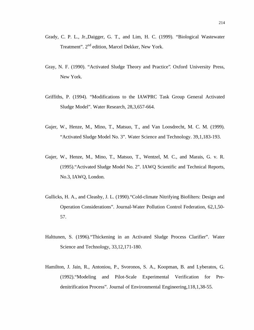
214
Grady, C. P. L., Jr.,Daigger, G. T., and Lim, H. C. (1999). “Biological Wastewater
Treatment”. 2nd edition, Marcel Dekker, New York.
Gray, N. F. (1990). “Activated Sludge Theory and Practice”. Oxford University Press,
New York.
Griffiths, P. (1994). “Modifications to the IAWPRC Task Group General Activated
Sludge Model”. Water Research, 28,3,657-664.
Gujer, W., Henze, M., Mino, T., Matsuo, T., and Van Loosdrecht, M. C. M. (1999).
“Activated Sludge Model No. 3”. Water Science and Technology. 39,1,183-193.
Gujer, W., Henze, M., Mino, T., Matsuo, T., Wentzel, M. C., and Marais, G. v. R.
(1995).“Activated Sludge Model No. 2”. IAWQ Scientific and Technical Reports,
No.3, IAWQ, London.
Gullicks, H. A., and Cleasby, J. L. (1990).“Cold-climate Nitrifying Biofilters: Design and
Operation Considerations”. Journal-Water Pollution Control Federation, 62,1,50-
57.
Halttunen, S. (1996).“Thickening in an Activated Sludge Process Clarifier”. Water
Science and Technology, 33,12,171-180.
Hamilton, J. Jain, R., Antoniou, P., Svoronos, S. A., Koopman, B. and Lyberatos, G.
(1992).“Modeling and Pilot-Scale Experimental Verification for Pre-
denitrification Process”. Journal of Environmental Engineering,118,1,38-55.
215
Hanaki, K., Wantawin, C., and Ohgaki, S. (1990a).“Effects on the Activity of
Heterotrophs on Nitrification in a Suspended-Growth Reactor”. Water Research,
24,3,289-296.
Hanaki, K., Wantawin, C., and Ohgaki, S. (1990b).“Nitrification at Low Levels of
Dissolved Oxygen with and without Organic loading in a Suspended-Growth
Reactor”. Water Research, 24,3,297-302.
Hartley, K. J. (1985).“Operating the Activated Sludge Process”. Gutteridge Haskins &
Davey Pty. Let., Brisbane, Queensland, Australia.
Hasselblad, S., Bjoerlenius, B., and Carlsson, B. (1998).“Use of Dynamic Models to
Study Secondary Clarifier Performance”. Water Science and Technology,
37,12,207-212.
Hasselblad, S., and Xu, S. (1998).“Solids Separation Parameters for Secondary
Clarifiers”. Water Environment Research, 70, 7,1290-1294.
Haug, R. T., and McCarty, P. L. (1972).“Nitrification with Submerged Filters”. Journal-
the Water Pollution Control Federation, 44,11,2087-2102.
Healey, M. J. (1989).“Improvements in the Activated Sludge Process in the U.K. and
U.S.”. Journal-Water Pollution Control Federation, 61,4,446-451.
Henze, M. (1992).”Characterization of Wastewater for Modeling of Activated Sludge
Processes”. Water Science and Technology, 25,6,1-15.
216
Henze, M., Dupont, R., Grau, P., and Sota, A. (1993).“Rising Sludge in Secondary
Settlers Due to Denitrification”. Water Research, 27, 2,231-236.
Henze, M., Grady, C., Gujer, W., Marais, G., and Matsuo, T. (1986).“Activated Sludge
Model No. 1. IAWPRC Task Group on Mathematical Modeling for Design and
Operation of Biological Wastewater Treatment”. IAWPRC Scientific and
Technical Report No.1.
Henze, M., Gujer, W., Mino, T., Matsuo, T., Wentzel, M. C., and Marais, G. v. R
(1995a).“Activated Sludge Model No. 2”. IAWQ Scientific and Technical
Reports, No.3, IAWQ, London, UK.
Henze, M., Gujer, W., Mino, T., Matsuo, T., Wentzel, M.C., and Marais, G.v.R. (1995c).
“Wastewater and Biomass Characterization for the Activated Sludge Model No.2:
Biological Phosphorus Removal”. Water Science and Technology, 31,2,13-23.
Henze, M., Harremoes, P., Jansen, Jes la C., and Arvin, E. (1995b).“Wastewater
Treatment”. Springer-Verlag Berlin Heidelbert, Germany.
Henze, M., Gujer, W., Mino, T., Matsuo, T., Wentzel, M. C., Marais, G. v. R., and Van
Loosdrecht, M. C. M. (1999). “Activated Sludge Model No. 2D. IAWQ Task
Group on Mathematical Modeling for Design and Operation of Biological
Wastewater Treatment”. Water Science and Technology, 39,1,165-182.
Holmberg, A., and Forsstrom, J. (1984).“Application of Models in Developing Control
Strategies for Activated Sludge Wastewater Treatment Plants”. Water Science and
Technology, 16,5-7,587-594.

217
Horan, N. J., Parr, J., and Naylor, P. J. (1991).“Evaluation of Tracers for Determination
of the Mixing Characteristics of Activated Sludge Reactors”. Environmental
Technology, 12,603-608.
Huang, J., and Hao, O. J. (1996).“Alternating Aerobic-Anoxic Process for Nitrogen
Removal: Dynamic Modeling”. Water Environment Research, 68,1,94-104.
Huang, J. V. C., and Drew, D. M. (1985).“Investigation of the Removal of Organics and
Nitrogen in an Oxidation Ditch”. Journal-Water Pollution Control Federation,
57,2,151-156.
Hunze, M., Krause, K., and Obenaus, F. (2000). “Compartmentalization of A Surface-
Aerated Circulation Basin Using a 3-D Velocity Field”. 5th International
Symposium on Systems Analysis and Computing in Water Quality Management,
Gent, Belgium, September 18-20, 2000.
Iida, Y. (1988).”Performance Analysis of the Aeration Tanks in the Activated Sludge
System”. Water Science and Technology, 20,4/5,109-120.
Isaacs, S., Hansen, J. A., Schmidt, K., and Henze, M. (1995).“Examination of the
Activated Sludge Process No. 2 with an Alternating Process”. Water Science and
Technology, 31,2,55-66.
James, A. (1982).“Some Perspectives in the Modeling of Biological Treatment of
Wastewater”. Water Science and Technology, 14, 227-240.
218
Jansen, Jes la C., Nyberg, Ulf., Aspegren, H., and Andersson, B. (1993). “Handling of
Anaerobic Digester Supernatant Combined with Full Nitrogen Removal”. Water
Science and Technology, 27, 5-6, 391-403.
Jeppsson, U., and Diehl, S. (1996a).“An Evaluation of a Dynamic Model of the
Secondary Clarifier”. Water Science and Technology, 34,5-6,19-26.
Jeppsson, U., and Diehl, S. (1996b).“On the Modeling of the Dynamic Propagation of
Biological Components in the Secondary Clarifier”. Water Science and
Technology, 34,5-6,85-92.
Jones, G. L. (1973).“Bacterial Growth Kinetics: Measurement and Significance in the
Activated Sludge Process”. Water Research, 7, 7-12, 1475-1492.
Jones, M., and Stephenson, T. (1996). “The Effects of Temperature on Enhanced
Biological Phosphate Removal”. Environmental Technology, 17,965-976.
Kabouris, J. C., and Georgakakos, A. P. (1990).“Optimal Control of the Activated Sludge
Process”. Water Research, 24,10,1197-1208.
Keinath, T. M. (1985).“Operational Dynamics and Control of Secondary Clarifiers”.
Journal-Water Pollution Control Federation, 57,7,770-776.
Kerrn-Jespersen, J. P., and Henze, M. (1993).“Biological Phosphorus Uptake under
Anoxic and Aerobic Conditions”. Water Research, 27, 4,617-624.

219
Kim, Y., Pipes, W. O., and Chung, P. G. (1998).“Control of Activated Sludge Bulking by
Operating Clarifiers in a Series”. Water Science and Technology, 38, 8/9,1-8.
Knowles, B. (1982).“Denitrification”. Microbiology Reviews, 46, 1,43-67.
Koerner, H., and Zumft, W. G. (1989).“Expression of Denitrification Enzymes in
Response to the Dissolved Oxygen Level and Respiratory Substrate in Continuous
Culture of Pseudomonas Stutzeri”. Applied and Environmental Microbiology,
55,7,1670-1676.
Kokufuta, E., Shimohashi, M., and Nakamura, I. (1988).“Simultaneous Occurring
Nitrification and Denitrification under Oxygen Gradient by Polyelectrolyte
Complex-Coimmobilized Nitrosomonas Europaea and Paracoccus Denitrificans
Cells”. Biotechnology and Bioengineering, 31,2,382-384.
Kornaros, M., and Lyberatos, G. (1997).“Kinetics of Aerobic Growth of a Denitrifying
Bacterium, Pseudomonas Denitrificans, in the Presence of Nitrates and/or
Nitrites”. Water Research, 31,3,479-488.
Krebs, P. (1995).“Success and Shortcomings of Clarifier Modeling”. Water Science and
Technology, 31,2,181-191.
Krul, J. M., and Veeningen, R. (1977).“The Synthesis of the Dissimilatory Nitrate
Reductase under Aerobic Conditions in a Number of Denitrifying Bacteria
Isolated from Activated Sludge and Drinking Water”. Water Research, 11,6,39-
43.
220
Kuenen, J. G., and Robertson, L. A. (1994).“Combined Nitrification-Denitrification
Processes”. FEMS Microbiology Reviews, 15, 109-117.
Kumar, P., Mehrotrat, I., and Viraraghavan, T. (1998).“Temperature Responses of
Biological Phosphorus-Removing Activated Sludge”. Journal of Environmental
Engineering,124,2,192-196.
Laanbroek, H. J., Bodelier, P. L. E., and Gerards, S. (1994).“Oxygen Consumption
Kinetics of Nitrosomonas and Nitrobacter Grown in Mixed Continuous Cultures
at Different Oxygen Concentrations”. Archives of Microbiology, 161, 156-162.
Lai, W., and Berthouex, P. M. (1990).“Testing Expert System for Activated Sludge
Process Control”. Journal of Environment Engineering,116,5,890-909.
Lee, T. T., Wang, F. Y., and Newell, R. B. (1997).“On the Modeling and Simulation of a
BNR Activated Sludge Process Based on Distributed Parameter Approach”.
Water Science and Technology, 39,6,79-88.
Lee, T. T., Wang, F. Y., and Newell, R. B. (1999).“Dynamic Modeling and Simulation of
Activated Sludge Process Using Orthogonal Collocation Approach”. Water
Research, 33,1,73-86.
Lee, Y. W., Ong, S. K., and Sato, C. (1997).“Effects of Heavy Metals on Nitrifying
Bacteria”. Water Science and Technology, 36, 12,69-74.

221
Leeuw, E. J., Kramer, J. F., Bult, B. A., and Wijcherson, M. H. (1996).“Optimization of
Nutrient Removal with On-Line Monitoring and Dynamic Simulation”. Water
Science and Technology, 33,1,203-209.
Lessard, P. (1989). “Operational Water Quality Management: Control of Storm Water
Discharges”. Ph.D Thesis, Imperial College.
Lessard, P., and Beck, M. B. (1991).“Dynamic Modeling Of Wastewater Treatment
Process”. Environmental Science and Technology, 25,1,30-39.
Lewandowski, Z. (1982).“Temperature Dependency of Biological Denitrification with
Organic Materials Additions”. Water Research, 16,1,19-22.
Lijklema, L. (1973).“Models in Biological Wastewater Treatment: Objectives, Results,
Applicability”. Mathematical Analysis of Decision Problems in Ecology
(Proceedings of the NATO Conference, Istanbul, Turkey July 1973), Vol. 5 of
Lecture Notes in Biomathematics. A. Charnes and W. R. Lynn, Eds., Springer-
Verlag, Berlin, 1975, 174-203.
Loveless, J. E., and Painter, H. A. (1968).“The Influence of Metal Concentration and pH
Value on the Growth of a Nitrosomonas Strain Isolated from Activated Sludge”.
Journal of General Microbiology, 52,1-14.
Lumbers, J. P., Cook, S. C., and Thomas, G. A. (1989). “Modeling of Nitrification at the
Mogden Treatment Works”. Water Science and Technology, 21, 4/5,305-314.

222
Magara, Y., Nambu, S., and Utosawa, K. (1976). “Biological and Physical Properties of
an Activated Sludge on Settling Characteristics”. Water Research, 10,71-77.
Maier, W., and Krauth, K. (1988).“Optimizing Nitrification in Aeration Basins with
Surface Aerators”. Water Science and Technology, 20, 4/5, 23-28.
Matéju, V., Cizinska, S., Krejci, J., and Janoch, T. (1992).“Biological Water
Denitrification-A Review”. Enzyme Microbial Technology, 14,3,170-183.
Matsuo, Y. (1994). “Effect of the Anaerobic SRT on Enhanced Biological Phosphorus
Removal”. Water Science and Technology, 28,127.
Maurer, M., and Gujer, W. (1998).”Dynamic Modeling of Enhanced Biological
Phosphorus and Nitrogen Removal in Activated Sludge Systems”. Water Science
and Technology, 38,1,203-210.
Maurer, M., Gujer, W., Hany, R., and Bachmann, S. (1997).“Intracellular Carbon Flow in
Phosphorus Accumulating Organisms in Activated Sludge Systems”. Water
Research, 31, 4,907-917.
Mauret, M., Paul, E., Costes, E. P., Maurette, M. T., and Baptiste, P. (1996).“Application
of Experimental Research methodology to the Study of Nitrification in Mixed
Culture”. Water Science and Technology, 34, 1-2, 245-252.
Maurines-Carboneill, C., Morin, L., Pernelle, J .J., Derlet, N., Sachon, G., and Leblon, G.
(1998).“Reviviscence of Aerobic Chemo-heterotrophic Bacteria in an Activated

223
Sludge Pilot Plant After a Prolonged Absence of Oxygen”. Water Research, 32,
4,1213-1221.
Meiberg, J. B. M., Bruinenbert, P. M. m., and Harder, W. J. (1980).“Effects of Dissolved
Oxygen Tension on the Metabolism of Methylated Amines in Hyphomicrobium
in the Absence and Presence of Nitrate: Evidence for ‘Aerobic’ Denitrification”.
Journal of General Microbiology,120,453-463.
Milbury, W. F., McCauley, D., and Hawthorne, C. H. (1971).“Operation of Conventional
Activated Sludge for Maximum Phosphorus Removal”. Journal of Water
Pollution Control Federation, 43, 9-12, 1890-1901.
Mino, T., San Pedro, D. C., Yamamoto, S. and Matsuo, T. (1995).”Application of the
IAWQ Activated Sludge Model to Nutrient Removal Process”. Water Science and
Technology, 35,8,111-118.
Mino, T., Van Loosdrecht, C. M., and Heijnen, J. J. (1998).“Microbiology and
Biochemistry of the Enhanced Biological Phosphate Removal Process”. Water
Research, 32, 11,3193-3207.
Morris, J. W., Batchelder Adams, L. A., and Tozer, H. G. (1989).“Activated Sludge
Secondary Solids Flux Variability”. Journal-Water Pollution Control Federation,
61,1,73-82.
Mossakowska, A., Reinius, L., and Hultman, B. (1997).“Nitrification Reactions in
Treatment of Supernatant from Dewatering of Digested Sludge”. Water
Environment Research, 69, 6,1128-1133.
224
Muller, J.A. et al. (1967). “Floc Sizing Techniques”. Applied Microbiology,15,125-134.
Müller, A., Marsili-Libelli, S., Aivasidis, A., Lloyd, T., Kroner, S., and Wandrey, C.
(1997).“Fuzzy Control of Disturbances in a Wastewater Treatment Process”.
Water Environment Research, 31, 12,3157-3167.
Mulready,C.R., Payne,D.C., and Watkins,D.W. (1982). “A Comparison of the Carrousel
and Passveer Ditch Activated-Sludge Plant”. Water Pollution Control, 81, 297-
307.
Murnleitner,E.,Kuba,T., van Loosdrecht,M.C.M., and Heijnen,J.J. (1997). “An Integrated
Metabolic Model for the Aerobic and Denitrifying Biological Phosphorus
Removal”. Biotechnology and Bioengineering, 54,5,434-450.
Nakamura, K., Noike, T., Matsumoto, J. (1986).“Effect of Operation Conditions on
Biological Fe2+ Oxidation with Rotating Biological Contactors”. Water Research,
20, 1,73-77.
Newell, B., Bailey, J., Islam, A., Hopkins, L., and Lant, P. (1998).“Characterizing
Bioreactor Mixing with Residence Time Distribution (RTD) Tests”. Water
Science and Technology, 37, 12,43-47.
Nicolai, B. (1984).“Video Taping-A New Tool for Wastewater Operations”. Public
Works, 115,10,66.

225
Nielsen, J. L., and Nielsen, P. H. (1998).“Microbial Nitrate-Dependent Oxidation of
Ferrous Iron in Activated Sludge”. Environmental Science & Technology,
32,3556-3561.
Nielsen, M. K., Bechmann, H., and Henze, M. (1999). “Modeling and Test of Aeration
Tank Settling Ats”. 8th IAWQ Conference on Design, Operation and Economics
of Large Wastewater Treatment Plants, 6-9 September 1999, Budapest, Hungary.
Nielsen, M. K., and Onnerth, T. B. (1996).“Strategies for Handling of On-Line
Information for Optimizing Nutrient Removal”. Water Science and Technology,
33, 1, 211-222.
Nolasco, D. (1994).“Optimization of Nutrient Removal at a Large Facility with
Advanced Field Evaluation Tools and Dynamic Modeling”. Proceeding of the 67th
Annual Conference of Water Environment Federation, Chicago, I11, 1,619.
Nowak, O., Svardal, K., and Schweighofer, P. (1995).“The Dynamic Behavior of
Nitrifying Activated Sludge Systems Influenced by Inhibiting Wastewater
Compounds”. Water Science and Technology, 31, 2,115-124.
Olsson, G., and Andrews, J. F. (1978). “The Dissolved Oxygen Profile-A Valuable Tool
for Control of the Activated Sludge Process”. Water Research, 12, 985-1004.
Olsson, G. and Newell, B. (1999). “Wastewater Treatment Systems Modeling, Diagnosis
and Control”. IWA Publishing, London, UK.
226
O’Neil, M., and Horan, N. J. (1995).“Achieving Simultaneous Nitrification and
Denitrification of Wastewater at Reduced Cost”. Water Science and Technology,
32, 9-10, 303-312.
Orhon, D., Tasli, R., and Sozen, S. (1999).”Experimental Basis of Activated Sludge
Treatment for Industrial Wastewater-the State of the Art”. Water Science and
Technology, 40,1,1-11.
Orth, H. M., and Sapkota, D. P. (1988). “Upgrading a Facultative Pond by Implanting
Water Hyacinth”. Water Research WATRAG, 22, 12, 1503-1511.
Ossenbruggen, P. J., Spanjers, H., Aspegren, H., and Klapwijk, A. (1991).“Designing
Experiments for Model Identification of the Nitrification Process”. Water Science
and Technology, 24, 6,9-16.
Otterpohl, R. and Freund, M. (1992). “Dynamic Models for Clarifiers of Activated Sludge
Plants with Dry and Wet Weather Flows”. Water Science and Technology,
26,5/6,1391-1400.
Otterpohl, R., Rolfs, T., and Londong, J. (1994).“Optimizing Operation of Wastewater
Treatment Plants by Offline and Online Computer Simulation”. Water Science
and Technology, 30,2, 165-174.
Painter, H. A. (1977).“Microbial Transformation of Inorganic Nitrogen”. Progress in
Water Technology, 8, 4/5, 3-29.

227
Parker, D. S., Merrill, M. S., and Tetreault, M. J. (1992).”Wastewater Treatment Process
Theory and Practice: The Emerging Convergence”. Water Science and
Technology, 25,6,301-315.
Patry, G. G. and Chapman, D. (1989). “Dynamic Modeling and Expert Systems in
Wastewater Engineering”. Lewis Publishers, Chelsea, Michigan.
Peddie, C. C., Muvinic, D. S. and Jenkins, C. J. (1990). “Use of ORP for Monitoring and
Control of Aerobic Sludge Digestion”. Journal of Environmental Engineering,
116, 3, 461-471.
Peterson, W. (1985).“Contract Operations-One Alternative for Water Treatment
Facilities”. Journal of the North England Water Works Association, 99,1,62.
Pflanz, P. (1969). “Performance of Activated Sludge Secondary Sedimentation". In
Advances in Water Pollution Research (Edited by Jenkins S.H.), 569-581.
Pergamon Press, London.
Pitman, A. R., Trim, B. C., and van Dalson, L. (1988).“Operating Experience with
Biological Nutrient Removal at the Johannesburg Bushkipie Works”. Water
Science and Technology, 20, 4/5, 51-62.
Poduska, R. A., and Andrews, J. F. (1975).“Dynamics of Nitrification in the Activated
Sludge Process”. Journal-Water Pollution Control Federation, 47,11,2599-2619.
Pöpel, H. J., and Fischer, A. (1998a).“A New Comprehensive Concept for Modeling
Temperature Influences on Biological Treatment”. Proceedings of Water
228
Environment Federation 71st Annual Conference and Exposition, Orlando,
Florida, 1, 605.
Pöpel, H. J., and Fischer, A. (1998b).“Combined Influences of Temperature and Process
Loading on the Effluent Concentration of Biological Treatment”. Water Science
and Technology, 38, 8/9,129-136.
Prats, D., and Llavador, F. (1994).“Stability of Kinetic Models from Waste Stabilization
Ponds”. Water Research, 28, 10,2125-2132.
Priestley, M. (1981).“Spectral Analysis and Time Series”. (Sixth Printing, 1989), New
York: Academic Press.
Princince, A. B. (1995).“Minimizing Costs of Activated Sludge Systems: Application to
Deer Island Treatment Plant”. Proceeding of the 68th Annual Conference of Water
Environment Federation, Miami Beach, FL, 1,693.
Prosser, J. I. (1990).“Mathematical Modeling of Nitrification Processes”. Advances In
Microbial Ecology, 11, 263.
Randall, C. W., Barnard, J. L., and Stensel, H. D. (Eds.) (1992). “Design and Retrofit of
Wastewater Treatment Plants for Biological Nutrient Removal”. Technomics
Publishing, Lancaster, PA.
Randall, C. W., Benefield, C. D., and Buth, D. (1982).“The Effects of Temperature on
the Biochemical Reaction Rates of the Activated Sludge Process”. Water Science
and Technology, 14,1/2, 413-430.

229
Randall, C. W., and Buth, D. (1984).“Nitrite Buildup in Activated Sludge Resulting From
Temperature Effects”. Journal-Water Pollution Control Federation, 56,9,1039-
1043.
Reda, A. (1993). “Simulation and Control of Storm Water Impacts on River Water
Quality.” Ph.D Dissertation, Imperial College.
Rensink, C. W., Marshall, D. W., and King, P. H. (1981).“Biologische defosfatering en
procesbepalende factoren”. NVA Symposium Proceedings, Nieuwe
ontwikkelingen en praktijkervaringen in Nederland en Zweden.
Rittmann, B. E., and Langeland, W. E. (1985).“Simultaneous Denitrification with
Nitrification in Single-Channel Oxidation Ditches”. Journal-Water Pollution
Control Federation, 57,4,300-308.
Robert, M. A. (1983). “Procedures and Practices in Activated Sludge Process Control”.
Butterworth Publishers.
Rosen, B., and Morling, S. (1998).“A Systematic Approach to Optimal Upgrading of
Water and Wastewater Treatment Plants”. Water Science and Technology, 37,
9,9-16.
Rossman, L. A. (1984).“Effluent Ammonia Variability from Nitrification Plants”.
Proceeding of American Society of Civil Engineers, Environmental Engineering
Special Conference, 573.

230
Rouleau, S., Lessard, P., and Bellefleur, D. (1997). “Simulation of A Transient Failure in
A Wastewater Treatment Plant: A Case Study”. Water Science and Technology,
36, 5, 349-355.
Ryder, R. A. (1972). “Dissolved Oxygen Control of Activated Sludge Aeration”. Water
Research, 6, 441-445.
San, H. A. (1989).”A Kinetic Model for Ideal Plug-Flow Reactors”. Water Research,
23,5,647-654.
Satoh, H., Mino, T., and Matsuo, T. (1994).“Deterioration of Enhanced Biological
Phosphorus Removal by the Domination of Microorganisms without
Polyphosphate Accumulation”. Water Science and Technology, 30, 6,203-211.
Scheer, H., and Seyfried, C. F. (1997).“Enhanced Biological Phosphate Removal:
Modeling and Design in Theory and Practice”. Water Science and Technology,
35,10,43-52.
Scherfig, J., Schleisner, L., BrØnd, S., and Kilde, N. (1996).“Dynamic Temperature
Changes in Wastewater Treatment Plants”. Water Environment Research,
68,3/4,143-151.
Schutze, M., Butler, D., and Beck, M. B. (2000). “Parameter Optimization of Real-Time
Control Strategies for Urban Wastewater Systems”. 5th International Symposium
on Systems Analysis and Computing in Water Quality Management, Ghent,
Belgium, September 18-20, 2000. 3.17-3.24.

231
Sedory, P. E., and Stenstrom, M. K. (1995).“Dynamic Prediction of Wastewater Aeration
Basin Temperature”. Journal of Environmental Engineering,121,9,609-618.
Sen, D., and Schwinn, D. E. (1997).“Case Histories of Innovative Approaches to
Nitrogen Removal without New Tankage”. Proceeding of the 70th Annual Water
Environment Federation Conference and Exposition, Chicago, I11.
Serra, P., Sanchez, M., Lafuente, J., Cortes, U., and Poch, M. (1994).“DEPUR: A
Knowledge-based Tool for Wastewater Treatment Plants”. Engineering
Applications of Artificial Intelligence, 7,1,23-30.
Sharma, B. (1977).“Nitrification and Nitrogen Removal”. Water Research, 11, 7-12, 897-
925.
Shimizu, T., Kudo, K., and Nasu, Y. (1993).“Activated Sludge Process Performance
Using a Multistage Tower Aeration Tank”. Biotechnology and Bioengineering,
42,3,315-325.
Siegrist, H., and Gujer, W. (1994).“Nitrogen Removal in Activated Sludge Systems
Including Denitrification in Secondary Clarifiers”. Water Science and
Technology, 30, 6,101-111.
Siegrist, H., Krebs,P., Buhler, R., Purtschert, I., Rock, C., and Rufer, R. (1995).
“Denitrification in Secondary Clarifiers”. Water Science and Technology, 31,2,
205-214.
232
Siegrist, H., Krebs, P., Buehler, R., Purtschert, I., Roeck, C., and Rufer, R.
(1994).“Denitrification in Secondary Clarifier”. Water Science and Technology,
31,2,205-214.
Siegrist, H., and Tschui, M. (1992).”Interpretation of Experimental Data with Regard to
the Activated Sludge Model No. 1 and Calibration of the Model for Municipal
Wastewater Treatment Plants”. Water Science and Technology, 25,6,167-183.
Silverstein, J., and Schroeder, E. D. (1983).“Performance of SBR Activated Sludge
Processes with Nitrification/Denitrification”. Journal-Water Pollution Control
Federation, 55,4,377-382.
Simons, D. B., and Senturk, F. (1992). “Sediment Transport Technology: Water and
Sediment Dynamics”. Water Resources Publications.
Simpkin, T. J., and Boyle, W. C. (1988).“The Lack of Repression by Oxygen of the
Denitrifying Enzymes in Activated Sludge”. Water Research, 22, 2,201-206.
Skrinde, J. R., and Bhagat, S. K. J. (1982).“Industrial Wastes as Carbon Sources in
Biological Denitrification”. Journal-Water Pollution Control Federation,
54,4,370-377.
Smith,G.(1996). “Increasing Oxygen Delivery in Anoxic Tanks to Improve
Denitrification”. Proceedings of Water Environment Federation 69th Annual
Conference and Exposition, Dallas, Texas, 5, 345.

233
Smolders, G. J. F., Loosdrecht, M. C. M. van, Heijnen, J. J. (1995). “A Metabolic Model
for the Biological Phosphorus Removal Process”. Water Science and Technology,
31, 2,79-93.
Smolders, G. J. F., Meij, J. van der, van Loosdrecht, M.C.M., and Heijnen, J. J. (1994).
“Stoichiometric Model of the Aerobic Metabolism of the Biological Phosphorus
Removal Process”. Biotechnology and Bioengineering, 44, 837-848.
Snyder, S. W., Bazylinski, D. A., and Hollocher, T. C. (1987).“Loss of N2O Reductase
Activity as an Expression for Poor Growth of Psendomonas Aeruginosa on N2O”.
Applied and Environmental Microbiology, 53,9,2045-2049.
Solly, D., and Barr, K. (1997). “Optimize What You Have First! Low Cost Upgrading of
Plants for Improved Nutrient Removal”. Water Science and Technology,
39,6,127-134.
Sorour, M. T., Olsson, G., and Somlyody, L. (1993).“Potential Use of Step Feed Control
Using the Biomass in the Settler”. Water Science and Technology, 28,11-12,239-
248.
Spanjers, H., Vanrolleghem, P., Nguyen, K., Vanhooren, H., and Patry, G. G.
(1998).“Towards a Simulation-Benchmark for Evaluating Respirometry-Based
Control Strategies”. Water Science and Technology, 37, 12,219-226.
Spies, P. J., and Seyfried, C. F. (1988).“Ammonia Controlled Activated Sludge Process
for Nitrification-Denitrification”. Water Science and Technology, 20, 4/5, 29-36.

234
Srinath, E. G., Sastry, C. A., Pillai, S. C. (1959).“Rapid Removal of Phosphorus from
Sewage by Activated Sludge”. Experienta, 15, 339-340.
Stamou, A. I. (1994).”Modeling Oxidation Ditches Using the IAWPRC Activated Sludge
Model with Hydrodynamic Effects”. Water Science and Technology, 30,2,185-
192.
Stamou, A. I. (1997).“Modeling of Oxidation Ditches Using an Open Channel Flow 1-D
Advection-Dispersion Equation and ASM1 Process Description”. Water Science
and Technology, 36,5,269-276.
Steffens, M. A., lant, P. A., and Newell, R. B. (1997).“A Systematical Approach for
Reducing Complex Biological Wastewater Treatment Models”. Water Research,
31, 3, 590-606.
Stenstrom, M. K., and Song, S. S. (1991).“Effects of Oxygen Transport Limitation on
Nitrification in the Activated Sludge Processes”. Journal-Water Pollution Control
Federation, 63,3,208-219.
Stephens, H. L., and Stensel, H. D. (1998).“Effect of Operating Conditions on Biological
Phosphorus Removal”. Water Environment Research, 70, 3,362-369.
Stephensons, R. V., and Luker, M. (1994).“Full-Scale Demonstration of Nitrogen Control
by Operationally Modified Plug-Flow and Step-Feed Activated Sludge
Processes”. Proceeding of the 67th Annual Conference of Water Environment
Federation, Chicago, I11, 1,563.

235
Stokes, A. J., West, J. R., Forster, C. F., Kruger, R. C. A., Bel, M. de., and Davies, W. J.
(1997). “Improvements to a STOAT Model of a Full Scale Wastewater Treatment
Works Through the Use of Detailed Mechanistic Studies”. Water Science and
Technology, 36,5,277-284.
Stover, E. L., and Cown, B. W. (1985).“Making Treatment Plants Work”. Civil
Engineering, 55,3,64.
Strenstrom, M. K., and Song, S. S. (1991).“Effects of Oxygen Transport Limitation on
Nitrification in the Activated Sludge Process”. Research Journal of Water
Pollution Control Federation, 63, 208-219.
Surmacz-Górska, Joanna, Cichon, A., and Miksch, K. (1997). “Nitrogen Removal from
Wastewater with High Ammonia Nitrogen Concentration via Shorter Nitrification
and Denitrification”. Water Science and Technology, 36,10, 73-78.
Takacs, I. (1986). “Application of a Mathematical Model for Activated Sludge
Treatment”. Water Science and Technology WSTED4, 18, 6, 163-174.
Takacs, I., Patry, G. G., and Nolasco, D. (1991).“A Dynamic Model of the Clarification-
Thickening Process”. Water Research, 25,10,1263-1271.
Takacs, I., Patry,G. G.,Watson, B., and Gall, B. (1995). “Case Studies in Dynamic
Modeling of Large-scale Wastewater Treatment Plants”. Mathematical Modeling
of Systems, 1,3,185-198.
236
Tanthapanichakoon, W., and Himmelblam, D. M. (1981).”Simulation of a Time
Dependent Activated Sludge Wastewater Treatment Plant”. Water Research,
15,10,1185-1195.
Tasli, R., Artan, N., and Orhon, D. (1997).“The Influence of Different Substrates on
Enhanced Biological Phosphorus Removal in a Sequencing Batch Reactor”.
Water Science and Technology, 35, 1,75-80.
Temmink, H., Petersen, B., Isaacs, S., and Henze, M. (1996).“Recovery of Biological
Phosphorus Removal after Periods of Low Organic Loading”. Water Science and
Technology, 34,1-2,1-8.
Tench, H. B. (1994).“A Theory of the Operation of Full Scale Activated Sludge Plants”.
Water Research, 28,5,1019-1024.
Thomsen, J. K., Geest, T., and Cox, R. P. (1994).“Mass Spectrometric Studies of the
Effect of pH on the Accumulation of Intermediate in Denitrification by
Paracoccus denitrificans”. Applied and Environmental Microbiology, 60,2,536-
541.
Toerien, D.F. et al., (1990). “Enhanced Biological Phosphorus Removal in Activated
Sludge System”. Advances in Microbial Ecology, 11.
Tong, R. M., Beck, M. B., and Latten, A. (1980). “Fuzzy Control pf the Activated Sludge
Wastewater Treatment Process”. Automatica, 16, 659-701.
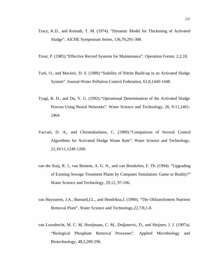
237
Tracy, K.D., and Keinath, T. M. (1974). “Dynamic Model for Thickening of Activated
Sludge”. AICHE Symposium Series, 136,70,291-308.
Trout, P. (1985).“Effective Record Systems for Maintenance”. Operation Forum, 2,2,18.
Turk, O., and Mavinic, D. S. (1989).“Stability of Nitrite Build-up in an Activated Sludge
System”. Journal-Water Pollution Control Federation, 61,8,1440-1448.
Tyagi, R. D., and Du, Y. G. (1992).“Operational Determination of the Activated Sludge
Process Using Neural Networks”. Water Science and Technology, 26, 9-11,2461-
2464.
Vaccari, D. A., and Christodoulatos, C. (1989).“Comparison of Several Control
Algorithms for Activated Sludge Waste Rate”. Water Science and Technology,
21,10/11,1249-1260.
van der Kuij, R. J., van Bentem, A. G. N., and van Brenkelen, F. Th. (1994). “Upgrading
of Existing Sewage Treatment Plants by Computer Simulation: Game or Reality?”
Water Science and Technology, 29,12, 97-106.
van Huyssteen, J.A., Barnard,J.L., and Hendriksz,J. (1990). “The Olifantsfontein Nutrient
Removal Plant”. Water Science and Technology,22,7/8,1-8.
van Loosdrecht, M. C. M, Hooijmans, C. M., Drdjanovic, D., and Heijnen, J. J. (1997a).
“Biological Phosphate Removal Processes”. Applied Microbiology and
Biotechnology, 48,3,289-296.
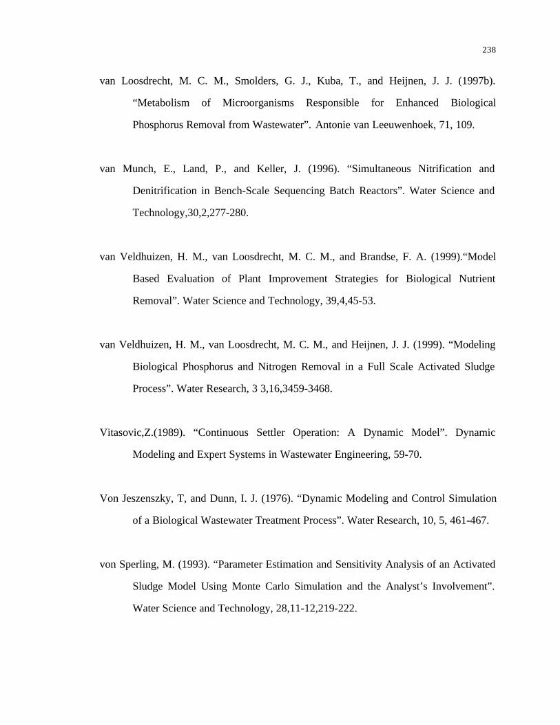
238
van Loosdrecht, M. C. M., Smolders, G. J., Kuba, T., and Heijnen, J. J. (1997b).
“Metabolism of Microorganisms Responsible for Enhanced Biological
Phosphorus Removal from Wastewater”. Antonie van Leeuwenhoek, 71, 109.
van Munch, E., Land, P., and Keller, J. (1996). “Simultaneous Nitrification and
Denitrification in Bench-Scale Sequencing Batch Reactors”. Water Science and
Technology,30,2,277-280.
van Veldhuizen, H. M., van Loosdrecht, M. C. M., and Brandse, F. A. (1999).“Model
Based Evaluation of Plant Improvement Strategies for Biological Nutrient
Removal”. Water Science and Technology, 39,4,45-53.
van Veldhuizen, H. M., van Loosdrecht, M. C. M., and Heijnen, J. J. (1999). “Modeling
Biological Phosphorus and Nitrogen Removal in a Full Scale Activated Sludge
Process”. Water Research, 3 3,16,3459-3468.
Vitasovic,Z.(1989). “Continuous Settler Operation: A Dynamic Model”. Dynamic
Modeling and Expert Systems in Wastewater Engineering, 59-70.
Von Jeszenszky, T, and Dunn, I. J. (1976). “Dynamic Modeling and Control Simulation
of a Biological Wastewater Treatment Process”. Water Research, 10, 5, 461-467.
von Sperling, M. (1993). “Parameter Estimation and Sensitivity Analysis of an Activated
Sludge Model Using Monte Carlo Simulation and the Analyst’s Involvement”.
Water Science and Technology, 28,11-12,219-222.

239
Wang, J. C., and Park, J. K. (1998).“Effect of Anaerobic/Aerobic Contact Time on the
Change of Internal Storage Energy in Two Different Phosphorus-Accumulating
Organisms”. Proceeding of the Water Environmental Federation 71st Annual
Conference & Exposition, Orlando, Florida, 1,129.
Watson, B., Rupke, M., Takacs, I., and Patry, G. (1994).“Modeling of Full-Scale
Wastewater Treatment Plants: How Detailed should it be?” Water Science and
Technology, 30,2,141-147.
Watts, J. D., and Cavenor-Shaw, A. R. (1998).“Process Audit and Asset Assessment
Using Online Instrumentation”. Water Science and Technology, 37, 12,55-61.
Wentzel, M. C., Ekama, G. A., and Marais, G. v. R. (1991).“Kinetics of Nitrification
Denitrification Biological Excess Phosphorus Removal Systems-A Review”.
Water Science and Technology, 23,4/6,555-565.
Wentzel, M. C., Ekama, G. A., and Marais, G. v. R. (1992).“Processes and Modeling of
Nitrification Denitrification Biological Excess Phosphorus Removal Systems-A
Review”. Water Science and Technology, 25,6,59-82.
Wentzel, M. C., Lotter, L. H., Loewenthal, R. E., and Marais, G. v. R. (1986).“Metabolic
Behavior of Acinetobacter sp. in Enhanced Biological Phosphorus Removal – A
Biochemical Model”. Water SA, 12, 209-224.
Werumeus Buning, W. G., Rijnart, F. W. A. M., and Weesendorp, P. P. (1991). “A
Systems Choice for Wastewater Treatment Systems for Biological Treatment of

240
Domestic Wastewater with Excessive N- and P-Removal”. Water Science and
Technology WSTED4, 24, 10, 231-237.
Wild, H. E., Sawyer, C. N., and McMahan, T. C. (1971).“Factors Affecting Nitrification
Kinetics”. Journal-Water Pollution Control Federation, 43,9,1845-1854.
Wild, D., Von Schulthess, R., and Gujer, W. (1995).“Structured Modeling of
Denitrification Intermediates”. Water Science and Technology, 31, 2,45-54.
Yang, L., and Alleman, J. E. (1992).“Investigation of Batchwise Nitrite Build-up by an
Enriched Nitrification Culture”. Water Science and Technology, 26, 5/6, 997-
1005.
Ydstebo, L., and Bilstad, T. (1997).“Experiences with Bio-P and BNR at Low
Temperature”. Proceeding of the 70th Annual Water Environment Federation
Conference and Exposition, Chicago, I11, 1,451.
Ye, R. W., Averill, B. A., and Tiedje, J. M. (1994).“Denitrification: Production and
Consumption of Nitric Oxide”. Applied and Environmental Microbiology,
60,4,1053-1058.
Young, P. C. (1984). Recursive Estimation and Time-series Analysis. Springer, Berlin.
Young, P. C., and Benner, S. (1991).“MicroCAPTAIN 2: User Handbook, First Edition,
Center for Research on Environment Systems”. Institute of Environmental and
Biological Sciences, Lancaster University, UK.

241
Young, P. C., and Beven, K. J. (1994).“Data-Based Mechanistic (DBM) Modeling and
the Rainfall-flow Nonlinearity”. Environmetrics, 5,3,335-363.
Young, P. C., Jakeman, A. J., and Post, D. A. (1997).“Recent Advances in the Data-based
Modeling and Analysis of Hydrological Systems”. Water Science and
Technology, 36, 5,99-116.
Young, P.C., and Lees, M. (1993).“The Active Mixing Volume: A New Concept in
Modeling Environmental Systems”. Statistics for the Environment. John Wiley
and Sons Ltd.
Yuan, Z., Vanrolleghem, P. A., and Vansteenkiste, G. C. (1997).“Modeling Error
Identification of Activated Sludge Models”. Water Science and Technology, 36,
5,81-88.
Zhong, J., McCorquodale, J. A., Zhou, S. P., and Vitasovic, Z. (1996).“A Dynamic Solids
Inventory Model for Activated Sludge Systems”. Water Environment Research,
68,3,329-337.
Zhou, S., and McCorquodale, J. A. (1992). “Modeling of Rectangular Settling Tanks”.
Journal of Hydraulic Engineering, ASCE, 118,10,1391-1405.
Zickefoose, C. S. (1981). “Activated Sludge Troubleshooting at the Pullman, Washington
WWTP”. Water Pollution Control Federation Highlights, 18, 1, 9 and 14-17.

242
APPENDIX I
QA/QC PROCEDURES FOR THE MONITORS
1. DATA DOWNLOADING
On a daily basis fresh data (detailed data & daily data) have to be FTPed from HP
workstation onto the personal computer. Then data, especially detailed data for each
individual instrument have to be checked for diagnostic purposes. Once malfunction of
instrument is spotted from the diagnostic information, laboratory visit is necessary to
correct the problem as soon as possible and then resume the normal operations.
2. NUMBERING OF THE TRAILERS AND INSTRUMENTS
The trailer housing ammonium monitor, TOC monitor, and suspended solids
monitor is numbered as trailer 1, while the other one with orthophosphate monitor, NOx
monitor is numbered as trailer 2. All the instruments coming with EPCL, either on-board
or out-board, are numbered in sequence as follows:
q Instrument #1: Respirometer 1 (trailer 1);
q Instrument #2: Data Logger 1 (trailer 1);
q Instrument #3: TOC/NH3/ Low Suspended Solid Monitor (outboard);
q Instrument #4: Respirometer 2 (trailer 2);
q Instrument #5: Data Logger 2 (trailer 2);
q Instrument #6: PO4 Monitor (trailer 2);
q Instrument #7: NOx Monitor (trailer 2);
q Instrument #8: Sludge Blanket Level Sensor (outboard);
q Instrument #9: External Double DO and MLSS Sensors (outboard).

243
3. LOCATIONS OF SAMPLE FLOWS AND THEIR NUMBERING
During the comprehensive sample campaign from 1 February, 1998 to 6 April,
1998, the locations of sample flows directed to each trailer and the numbering are as
follows:
Trailer 1
Stream 1–Tail end of the outer channel in the aeration tank #2;
Stream 2–Tail end of the middle channel in the aeration tank #2;
Stream 3–Tail end of the inner channel in the aeration tank #2 before disposal into the
secondary clarifier.
Trailer 2
Stream 1–Tail end of the inner channel in the aeration tank #2;
Stream 2–Tail end of the middle channel in the aeration tank #2;
Stream 3–Final effluent of the secondary clarifier before its being discharged into the
receiving water body.
4. DETAILED DATA CHECKING
The detailed data files have the extension of ".p*", where * represents the
instrument number.
4.1 Respirometers
Check the "DO" plot to see if the cycles are doing exactly as it is set up. And also
check to see if there is time gap between adjacent data files.

244
Figure 1. An Examplary ‘absolute d.o.” Curve of the Respirometer Detailed Data.
For example, if the respirometer is set up to run 11 DO cycles, one should be able
to see that much cycles in every single ‘absolute d.o.’ plot as shown if Figure 1.
4.2 TOC/NH3/ Low Suspended Solid Monitor
These three instruments are bundled together and numbered as instrument #3.
Since all three instruments can be accessed with the same keypad on the face of
ammonium monitor, if maintenance work is performed on one of the three instruments
the operations of the other two have to be temporarily suspended.

245
4.2.1 Ammonium Monitor
Figure 2. Detailed Data of the Ammonium Monitor
Shown in Figure 2 is the diagnostic information for the ammonium monitor. One
always has to make sure that ‘Diagnostic pH’ is over 11 such that all ammonium in the
samples is liberated into ammonia gas to be measured by the ammonia probe. Also make
sure that the ‘Diagnostic temperature’ stays constant at 40 degree centigrade.
The ammonium monitor performs self-calibration on two standard solutions on a
regular basis before taking any samples, ensuring that any following sample analysis is
sound. Calibration starts with the high standard solution (10 mg/L) and then goes to the
low standard solution (1 mg/L). During the calibration cycle, ammonium concentration
readings (mg/L) should stay constant and fairly close to the real standard solution
concentrations as shown in Figure 2.

246
4.2.2 TOC Monitor
Figure 3. Detailed Data of the TOC Monitor
Figure 3 shows the diagnostic information for the TOC monitor. Two signals in
this graph serve the diagnostic purposes. One is ‘Oxidisable C (mg/l)’, which is the
concentration of carbon that can be oxidized by a very strong oxidant. The other signal is
‘rip TOC (voltage)’. This monitor is calibrated against two standard solutions. One is
deionized water (0 mg/L), the other solution has a carbon concentration of 200 mg/L. So
the readings of "oxidisable C" should stay fairly constant at 0 and 200 mg/L. In the "rip
TOC" curve the "flat plane" near the end should stay stable.
4.3 External Double DO and MLSS Sensors
As shown in Figure 4, the ‘raw sat. DO’ signal should be over 80% saturation,
and the ‘autocal. DO’ signal should be automatically adjusted to somewhere around
100% saturation.
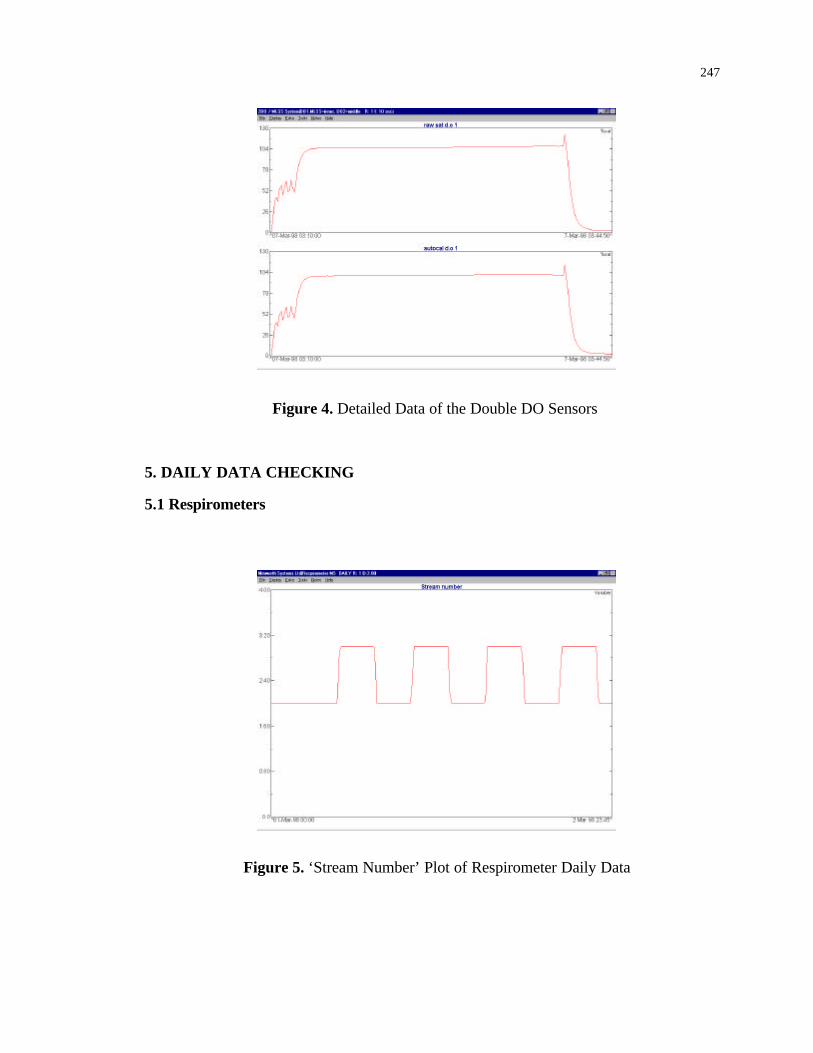
247
Figure 4. Detailed Data of the Double DO Sensors
5. DAILY DATA CHECKING
5.1 Respirometers
Figure 5. ‘Stream Number’ Plot of Respirometer Daily Data

248
The "stream number" plot as shown in Figure 5 is used to check whether there is
problem in flow switching due to blockage in any of the lines. If stream 1 is the current
sample flow, the curve should stay at 1.0. Likewise if stream 3 is the current sample flow,
the curve should stay at 3.0. If the curve stays at levels other than 1 or 3 when it should
be, blockage in sample lines needs to be cleared.
5.2 Ammonium Monitor
Figure 6. ‘Amm Delta Cal’ Plot of Ammonium Monitor Daily Data
As shown in Figure 6, the "ammonia delta cal" signal should be consistently over
50 mV.
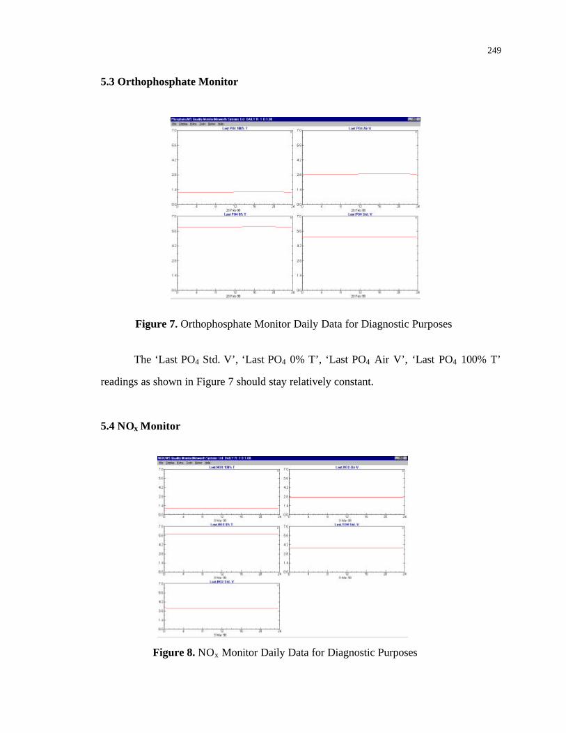
249
5.3 Orthophosphate Monitor
Figure 7. Orthophosphate Monitor Daily Data for Diagnostic Purposes
The ‘Last PO4 Std. V’, ‘Last PO4 0% T’, ‘Last PO4 Air V’, ‘Last PO4 100% T’
readings as shown in Figure 7 should stay relatively constant.
5.4 NOx Monitor
Figure 8. NOx Monitor Daily Data for Diagnostic Purposes

250
The ‘Last NO2 Std. V’, ‘Last TON Std V’, ‘Last NOx 0% T’, ‘Last NOx Air V’,
‘Last NOx 100% T’ readings as shown in Figure 8 should stay relatively constant.
251
APPENDIX II
DAILY MAINTENANCE CHECKLIST OF THE
INSTRUMENTS IN EPCL
1. SAMPLING SYSTEM
q Sampling collection & pumping
Rinse the collection drums with high-pressure hose daily.
q Observe sample loop condition and monitor discharge rates daily
q Ultrafilters
• Avoid buildup of debris in ultrafilter casings. When debris buildup is spotted,
stop the line and take the ultrafilter out for a clean;
Note: Avoid regular purging of sample loops with compressed air. Try to
avoid full-scale air blasts, since the ultrafilters are delicate.
• Monitor and record the suction pressure on each filtrate line & intervene
before the pressures become excessive.
2. RESPIROMETERS
q Wash respirometer tanks to remove excess fouling inside the walls;
q Keep the float switches as clean as possible. Better test the overflow level
switches periodically;
q Observe the filling rate of sample into the tank;
q Prevent mixer problems by cleaning any debris collected on the impeller;
q Clean and check the pH probe periodically.
252
3. TOC MONITOR
q Check reagents & standard solutions regularly, especially on Fridays;
q Look inside the enclosure for water leakages, which may indicate pump tube
failures;
q Check deflection of "U" tube water.
4. NH3 MONITOR
q Check reagents & standard solutions regularly, especially on Fridays;
q Check the free flow of sample, indicated by the ratio of air and sample in
scavenge pump inlet tube;
q Pulsing of sample feed tube is indicative of sample starvation;
q Look in tray for evidence of pump tube failure.
5. TURBIDITY MONITOR
q Check that the sample delivery line has no entrained air;
q Clean the debubbler with large bottle brush.
6. PO4 MONITOR
q Visually inspect for free delivery of sample & reagents;
q Check dilution water supply and replenish it if necessary;
q Check condition of deionizer cartridge.
7. NOX MONITOR
The same as those listed for PO4. Other than that, watch Cd column performance
and replace it when necessary.

253
8. EXTERNAL DOUBLE D.O PROBES
Inspect daily for gross fouling.
Note: Try to avoid over-maintaining, but should not neglect it either.
9. EXTERNAL MLSS PROBE
The same as those listed for external double DO probes. Other than that, calibrate
the external MLSS probe on a weekly basis.
10. SLUDGE BLANKET LEVEL SENSOR
Calibrate and inspect head of the sensor weekly. Make sure that the head is clean.