Rolling Contact Phenomena: Linear

Elasticity

J.J. Kalker*

*Department of Applied Mathematical Analysis, Delft University of Technology, The Netherlands

Abstract. In this paper, we treat the rolling contact phenomena of linear elasticity, withspecial emphasis on the elastic half-space.Section 1 treats the basics; rolling is defined, the distance between the deformable bod-ies is calculated, the slip velocity between the bodies is defined and calculated; a verybrief recapitulation of the theory of elasticity follows, and the boundary conditions areformulated.Section 2 treats the half-space approximation. The formulae of Boussinesq-Cerruti aregiven, and the concept of quasiidentity is introduced. Then follows a brief descriptionof the linear theory of rolling contact for Hertzian contacts, with numerical results, andof the theory of Vermeulen-Johnson for steady-state rolling. Finally, some examples aregiven.Section 3 is devoted to the simplified theory of rolling contact.In Section 4, the variational, or weak theory of contact is considered. First, we set up thevirtual work inequality, and it is shown that it is implied by the boundary conditions ofcontact. Then the complementary virtual work inequality is postulated, and it is shownthat it implies the boundary conditions of contact. Elasticity is introduced into bothinequalities, and the potential energy and the complementary energy follow. Finally,surface mechanical principles are derived.In Section 5, we return to the exact half-space theory. The problem is discretized, andsolved by means of the CONTACT algorithm. Finally, results are shown in Section 6.

1 Basics

In this Section, rolling is defined. Also, the distance between the bodies is calculated,the slip velocity between the bodies is defined and computed; a very brief recapitulationof the theory of elasticity follows, and the boundary conditions are formulated.

1.1 Definition of rolling

Consider two bodies of revolution. They are distinguished from each other by attachingto them the numbers 1 and 2. They are, for the time being considered as rigid. They

1

are pressed together so that they touch in a point; line contact will be treated presently.They are rotated, so that the contact point moves over the bodies. Then there are twopossibilities: either the velocity v1 of the contact point over body 1 equals the velocityv2 of the contact point over body 2, or this is not so. In the former case (equal velocities)one speaks of rolling, in the latter case one speaks of sliding or rolling with sliding.We consider the case that the bodies contact each other along a line. Again, the bodiesare rotated, and the line moves over the bodies. Rolling occurs when the velocities of thecontacting line over the bodies are equal at each point of the line, otherwise we speak ofsliding or rolling with sliding.We now consider that the bodies are deformable. First we have to define what we meanby that. We assume that each body is made up of particles that are glued together toform a continuum. Stresses and strains may be present in such a body. We count thedisplacement from an unstressed state in a manner which will be explained presently.The bodies are pressed together so that a contact patch forms between them, and theyare rotated. When the velocity v1 of the contact patch over body 1 almost equals thevelocity v2 of the contact patch over body 2 we speak of rolling, otherwise of sliding orrolling with sliding:

|v1 − v2| � |v1 + v2| (1)

(rolling, otherwise rolling with sliding).As we said, we count the displacement from the unstressed state, that is, the state inwhich there are no stresses acting in the bodies. A local Cartesian coordinate system isattached to each body. Each particle corresponds to a point y of the local coordinatesystem. The body is deformed; the displacement of the point y is denoted by w, functionof y and the time t. In the deformed state the particle lies in

y + w, w = w(y, t) (2)

We assume w small as well as its gradients:

|w| � |y|; |∂w/∂y| � 1 (3)

We assume that inertia terms may be neglected and that the deformation is elastic: thenwe arrive at a linearly elastostatic theory.We have two bodies; then we call the position ya in the a-th coordinate system, and thedisplacement wa.We want to compare the quantities of the bodies. To that end, we must refer them to asingle coordinate system. So we introduce a third, global coordinate system in which theparticles in the undeformed state are given by xa, and in the deformed state by xa +ua,that is, in the global coordinate system we also distinguish between the particles of body1 and body 2.The global coordinate system is connected to the two local systems by rotation matricesA(t) and the distance between the origins R(t) which are functions of the time. Therotation matrices are orthogonal matrices. Their columns are denoted by na, ta,ba. Let(1, 0, 0)T be given in the local system; then na is that same vector in the global system.Similarly, ta is the global representation of the vector (0, 1, 0)T in the local system, andba is the global representation of (0, 0, 1)T . It is easy to see that na, ta,ba indeed form

2

an orthonormal system.The following connection exists between the ya + wa and the xa + ua:

xa + ua = Aa(ya + Ra) + Aawa (4)

We identifyxa = (Aaya + Ra) ⇒ ya = AaT (xa −Ra) (5)

ua = Aawa(ya, t) ⇒ wa = Aaua (6)

In particular, (5) gives the global coordinate system in its dependence on the local coor-dinate system, and vice versa, and (6) defines the global displacement ua in terms of thelocal displacement wa, and vice versa.

It is clear from (5) that a variable belonging to body a can be written as a functionof xa and t or of ya and t.

Let ma be the outer normal on body a at ya; since wa is small with small gradients,ma is also the normal on the deformed body a at ya + wa. To see this, we assume thatthe surface of the body is given by F (y) = 0. Let z = y + w be the position of y in thedeformed state; that is, y = z−w. The deformed surface is then given by F (z−w) = 0.The normal m on the undeformed body at y is given by

m = ∂F/∂y (7)

The normal on the deformed body is

m′ = ∂F/∂z = (∂F/∂y)(∂y/∂z).

But

∂y/∂z = I − ∂w/∂z ≈ I ,

where I is the 3× 3 unit matrix. From this proposition it follows that m ≈ m′. In theglobal coordinates, ma becomes na, with

na = Aama (8)

The points y1 + w1 and y2 + w2 are in contact with one another when

x1 + u1 = x2 + u2, and n1 = −n2 (9)

Example: A rail surface consists of the union of a number of circular cylinders withparallel axes that touch one another. That is, the cylinders intersect and at the intersec-tion the first derivatives are continuous.

The equation of one circular cylinder is, in a Cartesian coordinate system (O;x,y,z)

(x− a)2 + (z − b)2 −R2 = 0, n = q(2(x− a), 0, 2(z − b))with the scalar q chosen so that n is a unit vector; then n is the unit normal on the rail.

3

1.2 The Distance

We assume that the bodies are not in contact at the point x, but that they are O(u)apart, and that the surface is smooth, all in the neighborhood of the point x, while therelation n1 = n2 is approximately valid. In a small neighborhood of x the bodies maybe visualized as two parallel slabs, see Fig. 1.

. .

..

xx +u1 1

1

Undef. surf. 2x2 +u2

x2

n

n

1

2

e h

Def. surf. 2

Undef. surf. 1

Def. surf. 1

Figure 1: The Distance

Let the distance between the slabs, (2) to (1), be h in the unstressed state, and e inthe deformed state. Then we have

h = n2T (x1 − x2), e = n2T {(x1 + u1)− (x2 + u2)} (10)

We simplify the expression for e. As we will see later on, the displacement occurs in alinearized contact problem such as we have here (small displacements, small displacementgradients) only in the form u1 − u2. We call this the displacement difference, and wedenote it by u. Introduction of the displacement difference into the expression for e, wefind

e = h+ n2T u = h− n1T u (11)

e: deformed, h: undeformed distance, (2) to (1).We analyze the deformed distance e.

• e > 0: there is a gap between the bodies at x1, x2; x = (x1 + x2)/2

• e = 0: the bodies are in contact at x;

• e < 0: the bodies penetrate at x. Impossible.

In sum, only e(x) ≥ 0 is possible.

In addition to the distance there is the play of forces. Contact tractions p1, p2

(dimension: N/m2) act on bodies (1) and (2). According to Newton’s Third Law,

p1 = −p2 .= p (12)

4

Then the normally directed traction on (1) at x, positive if compressive, is given by

pN = n2T (x)p Normal component (13)

and the tangential traction is given by

pT = p− n2pN (x) Tangential component (14)

When the bodies do not attract each other, the normal component of the traction vanishesoutside contact and is positive (=compressive) inside, while the deformed distance ispositive outside contact and vanishes inside. We can summarize this as follows:

e(x) ≥ 0 : either a gap or contact; (15)

pN (x) ≥ 0 : either no, or a compressive normal traction; (16)

epN = 0 (17)

In words, in contact, pN may be positive, and e = 0;outside contact, the normal traction vanishes, and e > 0.

We formalize this as follows. We choose a potential contact zone (also called thepotential contact area, pot.con.) which is such that

• The potential contact zone encompasses the real contact zone completely;

• In the potential contact zone pN ≥ 0, e ≥ 0, pNe = 0.

Note that the pot.con. may be chosen freely, as long as the above is satisfied.

Example: Consider a so-called Winkler bedding, i.e. a rigid flat plate upon whichare mounted springs. The springs are tangentially unconnected; they are equally longand have the same positive spring constant per unit area k m3/N in the normal direction:

n2T u1 = kpN , n2T u2 = −kpN , with k > 0⇒ e = h+ n2T u = h+ n2T (u1 − u2) = h+ 2kpN

Suppose that h > 0. Since pN ≥ 0 we must have that e ≥ h > 0, and hence pN = 0.Then e = h > 0, and n2T ua = 0, a = 1, 2.Suppose that h < 0. Since e ≥ 0 we must have that 2kpN = e − h > 0 ⇒ e = 0 and2kpN = −h > 0. Hence n2T u1 = −n2T u2. The solution is shown in Fig. 2.

5

N

k k k k k k k k k

F

Figure 2: Compression of a Winkler bedding (normal contact)

It is seen that the inequalities play an crucial role in determining the elastic field.This is typical of a contact problem.

1.3 The Slip

We determine the relative velocity of a particle of body 1 with respect to body 2.

Suppose that the particle y1 is in contact with the particle y2 at the time t, that is

x1(t) + u1(x1, t) = x2(t) + u2(x2, t)

If we denote time differentiation by a high dot, the velocity of particle 1 with respect tothe global coordinate system is

v1 = x1(t) + u1(x1, t) = x1(t) + (∂u1/∂x1)x1 + ∂u1/∂t (18)

v2 is similarly defined.

The slip s is the relative velocity of two particles in contact, that is,

s = v1 − v2 = {x1(t)− x2(t)}+ {u1(x1, t)− u2(x2, t)} (19)

Now,x1 = x2 + u2 − u2 ⇒ x1 ≈ x2 ≈ x

.= (x1 + x2)/2 (20)

so that, owing to the smallness of ua, and if x1 ≈ x2

s = x1 − x2 + (∂u1/∂x− ∂u2/∂x)x + ∂u1/∂t− ∂u2/∂t (21)

If x1 is not approximately equal to x2, then (x1−x2) is large with respect to {(∂ua/∂xa)xa+∂ua/∂t}, and s is also given by (21), albeit that the second and third terms are negligiblewith respect to the first.

6

We call

c = x1 − x2 creep (22)

v = −x rolling velocity (23)

u = u1 − u2 displacement difference (24)

s = c− (∂u/∂x)v + ∂u/∂t slip (25)

The minus sign in the definition of the rolling velocity calls for comment, see Fig. 3:

c

v

1

.x 2

x.

Figure 3: The definitions of creep and rolling velocity

Place the origin of the global coordinate system temporarily in x. Then x is thevelocity of the particles near x, and it is seen that the material flows backwards throughthe coordinate system, counter to the rolling direction. Hence the minus sign in thedefinition of the rolling velocity.

If a coordinate system may be found in which all quantities c, u, v are independentof the time t, one speaks of steady state rolling, otherwise of non-steady state rolling:

s = c− (∂u/∂x)v steady state rolling (26)

s = c− (∂u/∂x)v + ∂u/∂t non-steady state (or transient) rolling (27)

We finish this section on the slip by analyzing the creep for bodies of revolution that arerotated about their axes which are almost in the same plane. A number of interestingtechnological problems fall into this category.

1. Problems in which the contact area is almost flat. Examples:

(a) A ball rolling over a plane;

(b) An offset printing press: contact short in the rolling direction;

(c) An automotive wheel rolling over a road.

2. Problems with contact short in the rolling direction, curved in the lateral. Exam-ples:

7

(a) A railway wheel rolling over a rail;

(b) A ball rolling in a deep groove, as in ball bearings.

3. Problems in which the contact area is curved in the rolling direction, and conformingin the lateral direction. Example: a pin rolling in a hole.

1.4 Leading Edge, Trailing Edge

The contact region C has an edge. This edge consists of three parts: the leading edge,the trailing edge, and, possibly, a neutral edge. When the rolling velocity points outsidethe contact area at a point of the edge, this points belongs to the LEADING EDGE:particles move into the contact area with rolling velocity.

When the rolling velocity points into the contact region C at a point of the edge, thepoint belongs to the TRAILING EDGE: and particles leave the contact area at macro-scopic rolling velocity.

When the rolling velocity vanishes, or is parallel to the edge, we speak of a NEU-TRAL EDGE: particles move only into or outside the contact area through the elasticdeformation, not through the rigid body motion.

1.5 Example

We give an example of a simplified wheel-rail system. see Fig. 4.

z 1 11

O1

x

h (<0)h (>0)O

n

2n

1

x2

22 y

zy

xO 2

z

y

Figure 4: A simplified wheel-rail system

The origin O1 of the wheel lies on the axis of the cylinder (body 1). The origin O2

of the rail (body 2) lies on its surface. The origin O of the global coordinate system lieson the surface of the rail, perpendicularly below O1. It is contact fixed. The y-axis ofthe wheel coincides with the axis of the cylinder; it is the rotation axis of the wheel. They-axis of the global system coincides with the projection of the y-axis of the rail. Thex-axis is in the same sense as the rolling direction. The z-axis of the global system pointsvertically upwards. The sense of the y-axis is so that the global system is right-handed.The wheel rotates about its y-axis, clockwise, so that the wheel rolls over the rail to the

8

right.

We have

xa = Aaya + Ra ←→ ya = AaT (xa −Ra).xa is the global coordinate of the particle ya. Ra is the position of Oa in the globalcoordinates. The particle-fixed velocity at x is

xa = Aaya + Ra = AaAaT (xa −Ra) + Ra.This means: substitute xa,Ra,Ra in the right-hand side, and you find xa without calcu-lating ya.

Indeed we have:

BODY 1

R1 = (0, 0, r)T =⇒ R1 = 0

A1 =

+ coswt 0 + sinwt0 1 0

− sinwt 0 + coswt

;

A1 = w

− sinwt 0 + coswt0 0 0

− coswt 0 − sinwt

;

A1A1T = w

0 0 10 0 0−1 0 0

;

x1 = A1A1T (x1 −R1) =

wz − wr0−wx

.

BODY 2

x2 = y2 +

−vt00

=⇒ x2 =

−v00

When x = 0:

c = x1 − x2 =

v − wr00

; v = −(x1 + x2)/2 =

(v + wr)/200

c: creep at the origin, v: rolling velocity at the origin.

9

1.6 Recapitulation of the linear theory of elasticity

In the linear theory of elasticity it is more convenient to work with index notation thanwith matrix-vector notation. In index notation, the displacement ua (a = 1, 2: bodynumber) is denoted by its components ua

i , i = 1, 2, 3, in a Cartesian coordinate system.The body number a is omitted when no confusion may arise. Partial differentiation withrespect to the coordinate xj is denoted by ,j :

ui,j.= ∂ui/∂xj , the displacement gradient (28)

summation over 1,2,3 of repeated subscripts is understood. This summation conventionis undone by placing one or more subscripts between brackets.

As usual, we work in a small displacement, small displacement gradient theory. Thelinearized stresses are defined as

eij = (ui,j + uj,i)/2 = eji, (29)

and the stress is given by σij . The equations of equilibrium are

σij = σji and σij,j = 0 (30)

where we disregard inertial forces such as gravity in the rightmost equation. The surfaceload, also called the surface traction, is pi = σijnj , where nj is the outer normal on thesurface.

According to Hooke’s Law there is a linear relationship between the stresses σij andthe strains ehk. In the general case, this relation reads

σij = Eijhkehk, Eijhk : elastic constants (31)

and in the case of an isotropic material

eij =1 + ν

Eσij −

ν

Eδijσkk , σij =

Eeij

1 + ν+

Eδijekk

(1 + ν)(1− 2ν)(32)

with

E: Young’s Modulus, ν: Poisson’s Ratio, (elastic constants)

δij : Kronecker delta, =0 when i 6= j, =1 when i = j.

1.7 Friction

When two bodies slide over each other, it will often be observed that this motion isopposed by a force. This is the phenomenon of friction; the force is called the force offriction. Usually a finite compensating force is needed to set a body sliding, while inmany experiments the friction force remains constant during sliding. So it is assumed

10

that the shearing force is bounded by a force bound g, which depends on the normalforce Fz , the magnitude of the sliding velocity V and other parameters, thus

g = g(Fz, V, ...), ...: other parameters; Fz : normal comp. of total contact force (33)

When the sliding velocity (the slip, in fact) vanishes, the tangential force may fall belowthe traction bound g in absolute value; when sliding occurs, the tangential force is at thetraction bound, and it opposes the slip:

|Fτ | < g(Fz , V, ...) (34)

Fτ : tangential component of total contact force, τ = 1, 2,

|Fτ | =√

F 21 + F 2

2

if V 6= 0 : Fτ = −gvτ/V, Greek index: tangential comp. (35)

vτ : tangential component of sliding velocity; V = |vτ |.

Coulomb [2] proposed that g is proportional to Fz with a constant of proportionalitycalled the coefficient of friction:

g(Fz, V, ...) = fFz Coulomb, 1785 (36)

In order to interpret (36) Archard proposed in [1] that the friction was primarily causedby the adhesion of the bodies to each other. The adhesion takes place at the tips of theroughnesses of the bodies, which are called the asperities. At these tips the bodies are incontact and they form junctions, the real contact surface Cr, as opposed to the apparentcontact area C which consists of the junctions and the region in between them. Archardshowed that the area of the real contact surface is proportional to Fz , the normal com-pressive force.

At the real contact surface the bodies are welded together by interatomic forces. Ow-ing to the sliding motion the welded asperities shear; eventually the welds break, andthe asperities form new welds with different partners. The shearing of the asperities isaccompanied by micro-plastic deformation, and also by the detachment of material par-ticles from the bodies, thus leading to wear. From this it is seen that friction and wearare closely connected phenomena.

Despite this bolstering of Coulomb’s Law, it is generally agreed by tribologists that(36) must be modified. The simplest modification is the introduction of two coefficientsof friction, one for non-sliding (fstat) and one for sliding (fkin), with

fstat > fkin (37)

This did not suffice for many researchers, and they proposed more complicated relation-ships for the coefficient of friction.

11

So far we considered the total contact force, and the global velocity in sliding. Incontact mechanics, however, we need a local form of the friction law. A very simpletheory suggests itself: instead of global quantities use local quantities, that is instead ofF use p, the local traction, and instead of the global sliding velocity V use the slip s:

|pτ | ≤ g(pz, |sτ |, ...)

if |sτ | 6= 0 =⇒ pτ = −gsτ/|sτ | (38)

pτ : tangential traction component

sτ : slip component, τ = 1, 2

This law was stated and experimentally confirmed by Rabinowicz [7]. It was usedearlier in theoretical work see [4], [6], [3], and [5]. The traction bound is taken as

g(pz, |sτ |, ...) = f(|sτ |, ...)pz (39)

and f is usually taken constant.

1.8 Boundary conditions

We recall Hooke’s Law:σij = Eijhkehk (40)

It is valid for all types of bodies. Sometimes it is possible to bring it in surface mechanicalform:

ui(x) =

∫

∂V

Aik(x,y)pk(y)dS (y (41)

where A(x,y) is the displacement at x due to a point load at y; it is called the InfluenceFunction. The influence function depends strongly on the form of the body. In 3D elas-ticity it has been calculated for a few forms, in particular the half-space.

The advantage of (41) over (40) resides in the fact that for a 3D body (41) is takenover its 2D boundary only, while (40) extends over its entire 3D iterior.

The surface of body a is divided into three parts.

• In Ap the surface load is prescribed as p.

• In Au the surface displacement is prescribed as u

• Ac is the potential contact zone. It was already defined below eq. (17).

We give here a slightly different definition of the potential contact zone, which is roughlyequivalent to the one given before. It reads as follows:

The potential contact zone can be freely chosen under the following conditions:

12

1. It must completely encompass the contact region;

2. In it, x1 − x2 = O(u);

3. In it, n1 ≈ −n2.

Then the following relations hold in the potential contact:

e(x) = h(x) + n2T u(x), u(x) = u1(x)− u2(x), e ≥ 0 (42)

pN (x) = n2T p1, pN ≥ 0, pNe = 0 (43)

where the fields in x1 and x2 are suitably extended to

x = (x1 + x2)/2. (44)

The region where e = 0 is called the contact zone (contact region, contact area, contactpatch). It is denoted by C. In it, pN ≥ 0.The region where e > 0 is called the exterior zone (.. region, .. area). It is denoted by E.In it, pN = 0. (42),(43) are the mathematical description of C ∪ E = Ac. As we saw inthe Example of the Winkler bedding, (42),(43) determine the solution of the frictionlessproblem completely and uniquely. The inequalities of (42),(43) play a crucial role in thedetermination of the contact area and the elastic field.The equation pNe = 0 is very important. In conjunction with the inequalities it meansthat when e > 0 =⇒ pN = 0 and vice versa.

We turn to the boudary conditions of friction.We had defined the tangential component of the slip in the contact zone as s = x1− x2 +u1 − u2.The contact area is divided into two parts, viz. the stick area (area of adhesion, ..zone,..region) H , where the tangential component of the slip vanishes, and the area (zone,region) of slip S, where this is not so. We have for the total boundary conditions in thepotential contact area Ac:

in H : |sT | = 0, |pT | ≤ g (45)

in S: |sT | 6= 0, pT = −gsT/|sT (46)

S ∪H = C, S ∩H = � (47)

in C: e = 0, pN ≥ 0 (48)

in E: p = 0, e > 0 (49)

C ∪ E = Ac, C ∩ E = � (50)

References of Section 1

[1] J.F. Archard (1957), Elastic deformation and the laws of friction.Proceedings of the Royal Society of London, Ser. A 243, p. 190-205.

13

[2] C.A. Coulomb (1785), Theorie des machines simples. Memoire de Mathematiqueet de Physique de l’Academie Royale, p. 161-342.

[3] F.W. Carter (1926), On the Action of a Locomotive Driving Wheel. Proceedingsof the Royal Society of London A 112 p. 151-157.

[4] C. Cattaneo (1938), Sul contatto di due corpi elastici: distribuzione locale deglisforzi. Accademia Nazionale Lincei Rendiconti Ser 6 XXVII p. 342-348, 434-436,474-478.

[5] H. Fromm (1927), Berechnung des Schlupfes beim Rollen deformierbaren Scheiben.Zeitschrift fur angewandte Mathematik und Mechanik 7 p. 27-58.

[6] R.D. Mindlin (1949), Compliance of elastic bodies in contact. Journal of AppliedMechanics 16, p. 353-383.

[7] E. Rabinowicz, Friction and Wear of Materials. John Wiley and Sons, New York.

14

2 The half-space approximation

One of the ways to attack a contact problem is by means of the FEM. Especially whenwe deal with 3D problems this is very time consuming. The BEM of (1.41) is a muchmore promising option, if it is at all feasible.

This is so when we deal with a homogeneous, isotropic elastic 3D half-space. Thisis of great technological importance, as many problems may be approximately solved byusing a half-space.

A half-space consists of all points on one side of a plane, the bounding plane. Forinstance, in a Cartesian coordinate system (O;x, y, z) a half-space may be defined by{(x, y, z) : z ≥ 0}. The contact field of two elastic bodies may be calculated by meansof half-spaces when the maximum diameter of the contact area is small with respect toa typical dimension of the bodies, such as their diameter or the minimum radius of cur-vature near the contact. Then, the elastic field in the contact part may be calculated byreplacing the body locally by a half-space. The boundary conditions are then of the realbody, but the elasticity equations are solved for the half-space. The situation is shownin Fig. 5.Examples of the cases where the half-space approximation is valid:

trac. free trac. free

field

c

small

A

similar fields

small elastic fieldelasticsmall

fieldelastic

Figure 5: The half-space approximation

A ball pressed onto a thick slab, tread contact in wheels and rails, see Fig. 6.

15

tread contactBall on slabWheel-rail

Figure 6: Examples of the half-space approximation

Properties of the half-space approximation are:

1. Many geometries are elastically alike.This is most important as it renders software written for half-spaces applicable tomany geometries. The relative ease of the half-space approximation leads one touse it even where one is apt to make serious errors.

2. The influence numbers Aik(x,y) can be calculated exactly by means of the formu-lae of Boussinesq [1] and Cerruti [2].Derivations of these formulae may be found in [6] and in [3].

We give these formulae. We denote the global coordinate system by (O;x, y, z) =(O;xi), i = 1, 2, 3. O lies in the surface of the half-space. The axes of x and y liein the surface of the half-space. The axis if x = x1 points in the rolling direction,the axis of z = x3 points vertically upwards into body 1, and y = x2 completesthe right-handed coordinate system. Moreover, we denote the components of ua

by uai = (ua, va, wa) and the components of the surface traction by pa by pa

i =(pa

x, pay, p

az).

Clearly, by Newton’s Third Law,

p1i = −p2

i.= pi (51)

(41) reads

uai (x) =

∫

∞

−∞

∫

∞

−∞

Aaij p

aj (x′, y′) dx′dy′ (52)

In body a, a = 1, 2 we have

Aa1,3 =

1

4πGa{ (x− x

′)|z|r3

− (1− 2νa)(x − x′)r(|z|+ r)

} (53)

Aa2,3 =

1

4πGa{ (y − y

′)|z|r3

− (1− 2νa)(y − y′)r(|z|+ r)

} (54)

Aa3,3 =

−(−1)a

4πGa{z

2

r3+

2(1− νa)

r} (55)

r =√

(x − x′)2 + (y − y′)2 + z2 (56)

16

The factor −(−1)a in (55) calls for comment. When a = 1, it equals unity. Thenthe z-axis points into the body, and the component w1 has the same direction asthe concentrated load p1

3 = p3. When a = 2, we must have the same formulae butin a coordinate system in which the z-axis points vertically downwards, while theaxes of x and y remain the same. Then one must invert the sign of z in all formulae(53)-(55), and one must reverse the sign of w as well.So we see that the displacements in bodies 1 and 2 due to a normal loading obeythe law

u1(x, y, z) = u2(x, y,−z)v1(x, y, z) = v2(x, y,−z)w1(x, y, z) = −w2(x, y,−z)

if px = py = 0

The displacement differences, which are prescribed in the normal and tangentialproblems, are

u(x, y) = u1(x, y, 0)− u2(x, y, 0) =

=1

4π{1− 2ν1

G1− 1− 2ν2

G2}

∫

∞

−∞

∫

∞

−∞

pz(x′, y′)

x′ − xR2

dx′dy′

v(x, y) = v1(x, y, 0)− v2(x, y, 0) =

=1

4π{1− 2ν1

G1− 1− 2ν2

G2}

∫

∞

−∞

∫

∞

−∞

pz(x′, y′)

y′ − yR2

dx′dy′

w(x, y) = w1(x, y, 0)− w2(x, y, 0) =

=1

2π{1− ν

1

G1+

1− ν2

G2}

∫

∞

−∞

∫

∞

−∞

pz(x′, y′)/Rdx′dy′ (57)

px = py = 0, R =√

(x′ − x)2 + (y′ − y)2Ga : modulus of rigidity, νa : Poisson’s Ratio:

Elastic constants of body a

We combine ν1, ν2 and G1, G2 in the following manner:

1/G = {(1/G1) + (1/G2)}/2 (58)

ν/G = {(ν1/G1) + (ν2/G2)}/2 (59)

K = (G/4){(1− 2ν1)/G1 − (1− 2ν2)/G2} (60)

It is easy to see that G lies between G1 and G2. In the case of elastic symmetry(= both bodies having the same elastic constants),

G = G1 = G2, ν = ν1 = ν2, K = 0 (61)

The constant K vanishes when there is elastic symmetry, and also when bothbodies are incompressible: Steel on Steel, Rubber on Steel. Its maximum is 0.5

17

but in practice it is mostly small, e.g. 0.03 for steel on brass, and 0.09 for steelon aluminium. In terms of the constants of (58)-(60), the displacement differencebecomes:

u(x, y) =K

πG

∫ +∞

−∞

pz(x′, y′)

x′ − xR

dx′dy′ (62)

v(x, y) =K

πG

∫ +∞

−∞

pz(x′, y′)

y′ − yR

dx′dy′ (63)

w(x, y) =1− νπG

∫ +∞

−∞

pz(x′, y′)/Rdx′dy′ (64)

px = py = 0 (65)

R =√

(x′ − x)2 + (y′ − y)2 (66)

The procedure for the tangential traction/displacement is very nearly the same.We have for the displacement due to the load px, second index of Aa

ij equal to 1:

Aa11 = (−(−1)a)

1

4πGa{(1/r) +

+1− 2νa

|z|+ r+

(x′ − x)2r3

− (1− 2νa)(x′ − x)2r[|z|+ r]2

} (67)

Aa21 = (−(−1)a)

1

4πGa{ (x

′ − x)(y′ − y)r3

+

− (1− 2νa)(x′ − x)(y′ − y)r[|z|+ r]2

} (68)

Aa31 = − 1

4πGa{ (x

′ − x)|z|r3

+(1− 2νa)(x′ − x)

r[|z|+ r]} (69)

The displacement due to a load py in the y direction, second index of Aaij equal to

2 is found by the interchange of x and y, u and v, px and py. The factor −(−1)a

calls for comment: we must take into account that the shearing tractions on thebodies have different signs, and that therefore u, v, w have different signs in the twobodies, but that w is taken in a coordinate system that has a z-axis with the othersign, so that the factor −(−1)a is neutralized for the vertical displacement w.

The total surface displacement differences u(x, y), v(x, y), w(x, y) become (note thatz = 0!)

u(x, y) =1

πG

∫

∞

−∞

∫

∞

−∞

{px(x′, y′)[1− νR

+(x′ − x)2

R3] +

+ py(x′, y′)

(x′ − x)(y′ − y)R3

+Kpz(x′, y′)

x′ − xR2

}dx′dy′ (70)

v(x, y) =1

πG

∫

∞

−∞

∫

∞

−∞

{px(x′, y′)(x′ − x)(y′ − y)ν

R3+

18

+ py(x′, y′)[

1− νR

+(y′ − y)2R3

] +Kpz(x′, y′)

y′ − yR2

}dx′dy′

w(x, y) =1

πG

∫

∞

−∞

∫

∞

−∞

{ −Kpx(x′, y′)x′ − xR2

+

− Kpy(x′, y′)

y′ − yR2

+ pz(x′, y′)

1− νR}dx′dy′ (71)

3. Quasiidentity.The half-spaces in contact are called quasiidentical, when K = 0:

Quasiidentity ⇐⇒ K = 0 (72)

When K = 0, the displacement differences u and v are not influenced by the normaltraction pz, and the displacement diference w is not influenced by the tangentialtractions px and py. Yet there is a coupling through the traction bound, viz.

|(px, py)| ≤ fpz, f : coefficient of friction. (73)

Thus we must act as follows:

Determine pz when px = py = 0 (Normal problem)

Determine px, py when g = fpz (Tangential problem) (74)

This is called the Johnson process. It is approximately valid whenK is small. WhenK 6= 0, we must act differently. We use the so-called Panagiotopoulos process:

(a) Set I = 0, and pIx = pI

y = 0

(b) Determine the compressive traction pIz with (pI

x, pIy) as the tangential traction,

by means of a normal (= compressive traction) contact algorithm.

(c) Determine the next tangential traction (pI+1x , pI+1

y ) with pIz as the compressive

traction, by means of a tangential contact algorithm.

(d) If (pI+1x , pI+1

y ) is close enough to (pIx, p

Iy), we stop, else we set I = I + 1, and

we restart at b.

The Panagiotopoulos process was used by Oden and Pires [7] to prove the existenceof the elastic field for elastostatic contact. I use it myself for 3D half-space contact,and for 2D contact of elastic and viscoelastic layered media. It can, apparently,always be made to converge, but sometimes one must perturb the discretization ofthe contact problem.

Remark: The Johnson process is a one-step Panagiotopoulos process.

4. Slip in the Half-Space.We had seen in Section 1 that the slip was given by

s = c− (∂u/∂x)v + ∂u/∂t

19

with s the slip

c the creep

u the displacement difference

v the rolling velocity

x the position

t the time.

In half-space rolling, we assume that the rolling takes place along the positive x-axiswith constant velocity V , and that the motion takes place in the contact plane, sothat

c = V (υx − ϕy, υy + ϕx)T (75)

v = (V, 0)T (76)

and

sx = V (υx − ϕy − ∂u/∂x+ ∂u/∂(V t)) (77)

sy = V (υy + ϕx− ∂v/∂x+ ∂v/∂(V t)) (78)

υx is called the longitudinal creepage, υy is called the lateral creepage, and ϕ iscalled the spin. Another word for creepage is creep ratio.We identify

∫ t

0

V t′dt′ = q, distance traversed (79)

and divide (77) and (78) by V , where we call

S = s/V, the relative slip (80)

When we replace the time variable t by the distance traversed q, and the slip s bythe relative slip S, then we see that the relative slip is independent of the rollingvelocity V . Since the relative slip has the same direction as the real slip, and theformula for the tangential traction in sliding depends only on that direction whenthe coefficient of friction is independent of the rolling velocity (as we will assume),the entire problem becomes independent of the rolling velocity, or, more precisely,depends on the rolling velocity only through the coefficient of friction.

20

2.1 The Hertz Problem

Consider two paraboloids with parallel axes, numbered 1 and 2, see Fig. 7.

(1)

(2)

x

z

xyz

F

F

R

R(2)

(1)

x

xz

Figure 7: The Hertz problem

They are brought together so that their tips touch. A Cartesian coordinate systemis introduced in which the plane of x and y is the common tangent plane, the origin Olies in the tangent point, and the z-axis points vertically upwards into paraboloid 1. Weassume for simplicity that the planes of principal curvature coincide with one anotherand with the planes of x and y, as is often the case in rolling. The radii of curvature in

the plane of x are R(1)x and R

(2)x and those in the plane of y are R

(1)y , R

(2)y . We count

them positive when the centre of curvature lies inside the corresponding paraboloid.The bodies are compressed over a distance q. The problem is:FIND THE CONTACT AREA AND THE PRESSURE DISTRIBUTION WHEN FRIC-TION IS ABSENT OR IN THE CASE OF QUASIIDENTITY.

We choose the unstressed state so, that the displacements and the stresses vanish atinfinity. Then the equation of the surface of body a is

z(a) = −(−1)a{ x2

2R(a)x

+y2

2R(a)y

} − q(a) (81)

In the contact region, we have that

h = z(1) − z(2) = Ax2 +By2 − q (82)

with

A =1

2R(1)x

+1

2R(2)x

(83)

B =1

2R(1)y

+1

2R(2)y

(84)

q = q(1) − q(2) (85)

1

R=

A+B

2(86)

Hertz [9], [10] assumed that the contact area was elliptic in the half-space approximation,with

C = {(x, y, 0)|(x/a)2 + (y/b)2 ≤ 1} (87)

21

Then it may be shown that the normal pressure is semi-ellipsoidal

pz(x, y) = Gf00√

1− (x/a)2 − (y/b)2 (88)

where G and ν are the combined modulus of rigidity and the Poisson’s ratio, see (58),(59).The total normal force is found by integration of (88)

N =

∫ ∫

C

pzdxdy = (2/3)πabGf00, f00 =3N

2πabG(89)

The minor and the major semi-axes of the contact ellipse are denoted by S and L, andthe axial ratio by m′ = S/L:

m′ = S/L, S = min (a, b), L = max (a, b) (90)

The excentricity is signed. We have

|m| =√

1−m′2, m > 0 if a < b, m < 0 if a > b (91)

Then q, A and B are given by

q =3N(1− ν)SK

2πabG(92)

A(|m|) = B(−|m|) =3N(1− ν)(D −m2C)

2πabSG(93)

B(|m|) = A(−|m|) =3N(1− ν)(1−m2)D

2πabSG(94)

where K, B and D are complete elliptic integrals. We will encounter more completeelliptic integrals. They can all be expressed as a linear combination of two of them, forwhich we take C and D:

B =

∫ π/2

0

cos2 t√

1−m2 sin2 tdt,B = D−m2C (95)

C =

∫ π/2

0

sin2 t cos2 t√

1−m2 sin2 t3 dt (96)

D =

∫ π/2

0

sin2 t√

1−m2 sin2 tdt (97)

E =

∫ π/2

0

√

1−m2 sin2 tdt, E = (2−m2)D−m2C (98)

K =

∫ π/2

0

1√

1−m2 sin2 tdt, K = 2D−m2C (99)

We give these functions in their dependence on m′ in Table 1, taken from [4].

22

m’ B C D E K m2

↓ 0 1 -2+ln 4/m’ -1+ln 4/m’ 1 +ln 4/m’ 1.000.1 0.9889 1.7351 2.7067 1.0160 3.6956 0.990.2 0.9686 1.1239 2.0475 1.0505 3.0161 0.960.3 0.9451 0.8107 1.6827 1.0965 2.6278 0.910.4 0.9205 0.6171 1.4388 1.1507 2.3593 0.840.5 0.8959 0.4863 1.2606 1.2111 2.1565 0.750.6 0.8719 0.3929 1.1234 1.2763 1.9953 0.640.7 0.8488 0.3235 1.0138 1.3456 1.8626 0.510.8 0.8267 0.2706 0.9241 1.4181 1.7508 0.360.9 0.8055 0.2292 0.8491 1.4933 1.6546 0.191.0 .7864=π

4 .1964= π16 .7854=π

4 1.571=π2 1.571=π

2 0.00

Table 1: Complete elliptic integrals (Jahnke-Emde, 1943)[4]

It is seen from Table 1 that D > C, and it follows from (93) and (94) that A(|m| =B(−|m|) ≥ A(−|m|) = B(|m|), so that we have

A ≥ B =⇒ m ≥ 0, a ≤ b (100)

A ≤ B =⇒ m ≤ 0, a ≥ b (101)

A,B : see (86)

In order to find the excentricity of the contact ellipse, we set with Hertz [9]

cos t =|A−B|A+B

, with R =2

A+B(102)

and it follows from (93),(94), the fact that D > C and the expression of E in D and C

thatcos t = m2(D−C)/E (103)

We give the axial ratio m′ as a function of t in Table 2.

t 90o 80o 70o 60o 50o 40o 30o 20o 10o 0o

m′ = S/L 1.00 .79 .62 .47 .36 .26 .18 .10 .05 0

Table 2: The axial ratio of the contact ellipse as a function of t.

Table 2 is taken from [6] (page 197). We see from (86) to (103) that the shape ofthe contact ellipse depends only on the radii of curvature of the bodies, and not on theapplied load nor the elastic properties. The size of the contact area does, however:

A+B =2

R=

3N(1− ν)E2GπabS

(104)

or3N(1− ν)RE = 4πabSG (105)

23

A frequently used quantity is f00, see (88). Gf00 is the maximum value of the ellipsoidalpressure distribution pz(x, y). It is

f00 =3N

2πabG=

2S

(1− ν)RE(106)

Finally we determine the deepest penetration of the bodies, see (82):

q = (1− ν)KSf00 =2S2K

RE(107)

2.1.1 The linear theory of rolling contact for Hertzian contacts

We recall the formulae for the relative slip s/V in steady state rolling:

Sx = sx/V = υx − ϕy − ∂u(x, y)/∂x (108)

Sy = sy/V = υy + ϕx− ∂v(x, y)/∂x (109)

with

V : the rolling velocity

υx, υy, ϕ : longitudinal, lateral, spin creepage

(u, v) : tangential displacement difference, body (1)-(2)

x-axis : rolling direction

z-axis : vertical direction pointing into body (1)

y-axis : completes right-handed system

O : origin in centre of contact patch (ellipse)

When the creepages are very small, it is easy for (u, v) to compensate them, withoutviolating the traction bound. That is, almost the entire contact patch will be covered bythe stick region. Instead of saying that the creepages are small, one can also say that thecoefficient of friction goes up to infinity. Then the traction bound will not be violated aslong as (px, py) is finite. Now for finite (u, v) the traction is finite except maybe on theedge of the elliptic contact area, as it may be shown that the traction has inverse squareroot behaviour near the edge:

(px(x, y), py(x, y)) = O(√

1− (x/a)2 − (y/b)2−1

) (110)

so that the slip is confined to part of the edge of the contact area.

Hence inside the contact patch we have

∂u(x, y)/∂x = υx − ϕy, ∂v(x, y)/∂x = υy + ϕx (111)

Integrating with respect to x we find

u(x, y) = υxx− ϕxy + k(y) in C (112)

v(x, y) = υyx+ ϕx2/2 + l(y) in C (113)

px(x, y) = py(x, y) = 0 in E (114)

24

where k and l are arbitrary functions of y.

The question arises, how to determine k and l. We observe that (112) to (114) fullydetermine the contact problem together with the proper behaviour at infinity, where theelastic field has died out according to the half-space hypothesis.To that end, we observe that at the leading edge of the contact ellipse the traction mustvanish. For at the leading edge unloaded material flows into the contact patch. Duringtransit of the contact patch, traction builds up, which is suddenly released at the trailingedge. So at the leading edge the traction must vanish, but it need not do so at the trailingedge. Hence k and l must be determined so that the traction vanishes at the leadingedge, which is given by

{(x, y, z)|x ≥ 0, z = 0, |y| = b√

1− (x/a)2} leading edge (115)

We explain why this theory is called the Linear Theory. When we consider (112)-(114),and multiply υx, υy, ϕ, k, l with the same constantD, then it is clear thatD(px, py) satisfythe no-slip contact conditions with D(px, py) = (0, 0) on the leading edge. So the no-sliptangential traction corresponding to D(υx, υy, ϕ) is D(px, py) – a linear relationship.

At this place, we will not enter into the details of the calculation, but merely mentionthe result. We tabulate the total tangential force (Fx, Fy) and the twisting moment Mz

in terms of the creepages, as follows:

Fx =

∫ ∫

C

pxdxdy, Fy =

∫ ∫

C

pydxdy, (116)

Mz =

∫ ∫

C

(xpy − ypx)dxdy (117)

Fx = −GabC11υx, Fy = −GabC22υy −G(ab)1.5C23ϕ, (118)

Mz = −G(ab)1.5C32υy −G(ab)2C33ϕ (119)

with

Fx, Fy,Mz : total force and moment on body 1 (120)

υx, υy, ϕ : creepage (relative rigid slip) of body 1 wrt.body 2 (121)

This form of the total forces and the twisting moment follows from symmetries, while itis an empirical fact that

C11 > 0, C22 > 0, C23 = −C32 > 0, C33 > 0 (122)

These creepage and spin coefficients are tabulated in Table 3. The creepage and spincoefficients can be calculated in a purely numerical way. They can also be calculatedmore accurately in a semi-analytical way; these more accurate results are shown here.

25

a/b C11 C22 C23 = −C32 C33

ν = 0 0.5 ν = 0 0.5 ν = 0 0.5 ν = 0 0.50.1 2.51 4.85 2.51 2.53 .334 .731 6.42 11.70.2 2.59 4.81 2.59 2.66 .483 .809 3.46 5.660.3 2.68 4.80 2.68 2.81 .607 .889 2.49 3.720.4 2.78 4.82 2.78 2.98 .720 .977 2.02 2.770.5 2.88 4.83 2.88 3.14 .827 1.07 1.74 2.220.6 2.98 4.91 2.98 3.31 .930 1.18 1.56 1.860.7 3.09 4.97 3.09 3.48 1.03 1.29 1.43 1.600.8 3.19 5.05 3.19 3.65 1.13 1.40 1.34 1.420.9 3.29 5.12 3.29 3.82 1.23 1.51 1.27 1.271.0 3.40 5.20 3.40 3.98 1.33 1.63 1.21 1.161/.9 3.51 5.30 3.51 4.16 1.44 1.77 1.16 1.061/.8 3.65 5.42 3.65 4.39 1.58 1.94 1.10 .9541/.7 3.82 5.58 3.82 4.67 1.76 2.18 1.05 .8521/.6 4.06 5.80 4.06 5.04 2.01 2.50 1.01 .7511/.5 4.37 6.11 4.37 5.56 2.35 2.96 .958 .6501/.4 4.84 6.57 4.84 6.31 2.88 3.70 .912 .5491/.3 5.57 7.34 5.57 7.51 3.79 5.01 .868 .4461/.2 6.96 8.82 6.96 9.79 5.72 7.89 .828 .3411/.1 10.7 12.9 10.7 16.0 12.2 18.0 .795 .228

Table 3: Table of the creepage and spin coefficients

2.1.2 The theory of Vermeulen and Johnson for steady state rolling

In 1964, Vermeulen and Johnson [8] gave a theory for steady-state rolling for pure creep-age (ϕ = 0). They assumed that the stick area was also bounded by an ellipse, with thesame axial ratio as the contact ellipse and the same orientation, see Fig. 8, but touchingthe contact ellipse at its foremost point.

26

Slip Adh.

Figure 8: Areas and slip and adhesion according to Vermeulen and Johnson

Based upon that, they derived the creepage-force law shown in Fig. 9, broken line.In the left figure, the dots and crosses are the experimental values of Vermeulen andJohnson. Kalker improved the theoretical curve a little by making use of the creepagecoefficients, and the result is shown in the left and right figure 9 by a drawn line. In theleft figure, the dots and crosses are the experimental results of Vermeulen and Johnson,and in the right figure they are a comparison with the results of the numerical programsFastsim (see Section 3) and Contact (see Section 4).

+

∆

+O

F

FZ

a/b = 0.276

a/b = 0.683

a/b = 1.570O

ν = 0.28

a/b = 2.470f

w’

+

∆

1.0

0.9

0.8

0.7

0.6

0.5

0.4

0.3

0.2

0.1

0.00.70.60.50.40.30.20.10 0.8 1.0 1.1 1.2

Vermeulen-Johnson "THEORETICAL CURVE"

OX

X

∆X

X

O

+O

∆

∆

∆

∆

O

+O

X

X+

∆

0.9

= 2.73

= 3.28

= 4.4422

22

C

C

C

C

22

f = 0.10 (estimated)

f = 0.18 ( " )

f = 0.19 ( " )

f = 0.12 ( " )

1.3

22

= 5.53

∆

F

Fzf

w’

1.0

0.9

0.8

0.7

0.6

0.5

0.4

0.3

0.2

0.1

0.00.70.60.50.40.30.20.10 0.8 1.0 1.1 1.20.9 1.3

ν = 0.28

a/b = 0.3

a/b = 0.7

a/b = 0.6O

a/b = 0.4X

+

∆

ξ

FASTSIM, all ν and axial ratiosdiscr. 50x50

= 0

ξ

η

ξ

= 0

= 0

= η

O

XO

+

+∆O

O+∆OX+∆

O∆

X+ ∆ X"THEORETICAL CURVE"∆

Figure 9: Results of Vermeulen and Johnson. Left, comparison with the experiment;right, comparison with Fastsim and Contact, Kalker (1990)

It is seen that the drawn line is a near perfect fit to the experiment, Contact andFastsim.It is of interest to have the equation of the drawn line.Let

ξ′.= −abGC11υx

3fFz(123)

η′.= −abGC22υy

3fFzwith (124)

Cii : Creepage coefficient of the linear theory, see Table 3 (125)

a, b : Semiaxes of contact ellipse, a in rolling direction (126)

27

G : Modulus of rigidity (127)

f : Coefficient of friction (128)

Fz : Total compressive normal force (129)

We setw′ = |(ξ′, η′)| (130)

and it equals

w′ = 1− [1− (F/fFz)]1/3 if F ≤ fFz, F = |(Fx, Fy)|

≥ 1 if F > fFz (131)

We have for the ”theoretical line”:

(Fx, Fy) = (F/w′)(ξ′, η′) (132)

F = fFz [1− (1− w′)3] if w′ ≤ 1 (133)

= fFz if w′ ≥ 1 (134)

The only difference between the definition of Kalker’s line and the line of Vermeulen-Johnson is that Vermeulen-Johnson derive their line analytically on the basis of theirdivision of the contact area in regions of stick and slip, and arrive then at a different setof creepage coefficients, whereas Kalker maintains the form of the line of Vermeulen andJohnson, but gives it the correct slope at the origin w′ = 0.Indeed we have for the linear theory:

F =∂F

∂w′|w′=0w

′ = 3fFzw′ =⇒

(Fx, Fy) = (F/w′)(ξ′, η′) = 3fFz(ξ′, η′) = −abG(C11υx, C22υy)

as it should be.

2.2 Examples

2.2.1 Klingel rolling

Klingel rolling is a phenomenon that takes place in railway wheel sets when the wheelsare conical. Then the wheel set may be modelled by a rigid double cone, the rails aremodelled by two parallel straight rigid knives 2b apart, upon which the wheel set ismoving. The theory can be extended to more realistic cases.It is observed that the wheel set is not moving in a straight line, but has rather asinusoidal motion. The situation is shown in Fig. 10. IT IS REQUIRED TO GIVE ANEXPLANATION OF THIS PHENOMENON, WHICH IS CALLED THE KLINGELMOTION.

28

period = 23.8 m

(b)(a)

right rail

left rail

wheelset

railrailz

y

Figure 10: a: The wheel set as a double cone on knife-like rails b: The sinusoidalmotion of the centre of the wheel set

A coordinate system is introduced in which the origin lies in the middle betweenof the rails, the x-axis points in the rolling direction along the rails, the z-axis pointsvertically upwards, and the y-axis completes the right-handed system, i.e. it points inthe lateral, left direction if one stands looking in the direction of x. Let the centre of thewheel set have coordinates (x, y,R), where we neglect the height difference of the centreof the wheel set due to the shift of the mid position over a distance y with respect to therails. The apex angle of the double cone is 2γ, a small angle, the radius of the doublecone in the mid-position y = 0 is R, so that the radius of the wheels are

radius of left wheel on rail = R+ γy

radius of right wheel on rail = R− γy

2b is the width of the track.The angular velocity of the wheel set about the y-axis is ω > 0. The angle that the axisof the wheel set makes with the y-axis is α, a small angle. We have, when there is noslip between the wheel set and the rails:

y/V = α; α = −ωγy/b ⇒ y = −ωγyV/b = −ω2γyR/b

withV = ωR = rolling velocity

Consequently,y = y0 cos(ωt

√

γR/b)

where y0 is the amplitude (integration constant), the phase is arbitrary, and the angularfrequency is ω

√

γR/b, hence the frequency is (ω√

γR/b)/(2π) Hz. The period on the

rails is 2πR/√

γR/b, and therefore independent of the angular velocity of the wheel set.A pilot numerical value of the period on the rails is found by setting

γ = 1/40, R = 0.5 m, b = 0.715 m =⇒ period = 23.8 m

Frequency at 100 km/h = 1.17 Hz

29

2.2.2 A ball between two surfaces

Consider two steel surfaces that are mounted on an axle so that they make an angleof 2γ with one another. A steel ball with radius R is placed between them. The flatsurfaces are rotated in such a way that the angle 2γ is conserved; a coordinate system isintroduced in which the z-axis points vertically upwards, the y-axis points horizontallyoutwards, the x-axis completes the right-handed system, and the origin O lies in thecentre of the ball. The motion of the planes is so that the origin of the coordinate systemis stationary.IT IS REQUIRED TO FIND THE TOTAL FORCE IN Y-DIRECTION, WHEN THERADIAL POSITION OF THE ORIGIN OF THE COORDINATE SYSTEM IS GIVEN.The situation is sketched in Fig. 11.

x O

γγ

R

y

z

N

r

1

2

3

Figure 11: A ball between two surfaces

This problem was investigated by Johnson [5] in 1959.The angular velocity of the upper plane is ω and that of the lower plane is −ω. Theball does not rotate about the vertical axis z, by the symmetry of the two contacts. Thespin creepage at the upper contact, (2)-(1), is −ω/V = −1/r, where r is the distancebetween the axis of rotation of the two surfaces and the centre of the ball, see Fig. 11and γ = R/r is taken small. V is the velocity of rolling at the upper contact. The spincreepage, (2)-(3), at the lower contact is the same. The radius of the circular contactpatch is a, the total normal force is N = 16a3G/(3R(1 − ν)), where R is the radius ofthe ball. So the total force in y-direction is, according to the linear theory,

F = 2Nγ + 2Ga3C23/r = Nγ[2− 2C23a3G/(NR)] =

= Nγ[2− 2 ∗ 3(1− ν)/16C23] = 1.6Nγ

when we take care to stop the lateral creepage.

2.2.3 Creepage and spin for a railway wheel set

A railway wheel set consists of two wheels mounted on an axle. The wheel surfacesconsist of a flange, a tread, and a throat in between; the tread has (almost) the form of

30

a cone, as well as the flange; the throat is more or less circular, see Fig. 12. The railconsists of foot, a web and a rail head, see also Fig. 12.

tread

flangethroat

head

root

web

Figure 12: A railway wheel and rail surface

Fig. 13 schematically shows the wheel set standing on the rails. A coordinate systemis introduced in which the origin lies in the centre of the wheel set, the z-axis pointsvertically upwards, the x-axis points along the rails in the rolling direction from left toright, and the y-axis completes the right-handed coordinate system, pointing to the leftif one is facing the rolling direction.

right wheel

y

right rail

left rail

rolling

axle

α

left wheel α.

Figure 13: The wheel set standing on the rails

We start with the lateral creepage. Let α be the small angle between the y-axis andthe centre line of the wheel set, shown positive in Fig. 13. The lateral creepage consistsof two components, one due to α and one due to y, the lateral velocity of the centre ofthe wheel set. We have that y/V is compensated in part by α:

υy = y/V − α (135)

Note that in Klingel rolling, the lateral creepage vanishes. Next we consider the longitu-dinal creepage. It consists of three parts: the creepage due to the difference of the rollingradii of the wheels, and the rotation of the wheel set about a vertical axis through itscentre, and the braking or accelerating motion of the wheel set as a whole. The longi-tudinal creepage depends on whether we consider the left or the right wheel. The firstcomponent reads ω(Rleft − Rright)/V , where Rleft and Rright are the radii of left andright wheel, which depend on the lateral coordinate y, and V is the rolling velocity of thecentre of the wheel set. It compensates the longitudinal creepage, and it changes sign

31

with the wheel.The second component reads −αb/V ; it changes sign with the wheel.The third component reads (V −ωRmean)/V ; it does not change sign with the wheel. Intotal, we have for the longitudinal creepage in the left wheel

υx,left =−ω(Rleft −Rright)− αb+ (V − ωRmean)

V(136)

and in the right wheel

υx,right =ω(Rleft −Rright) + αb+ (V − ωRmean)

V(137)

Finally we consider the spin. It consists of two components, the kinematic spin and thegeometric spin.The kinematic spin is due to the rotation of the wheel set about the vertical axis. Itequals α/V , and it is the same for both wheels.The geometric spin is due to the conicity of the wheels, see Fig. 14. The conicity of thewheels is γleft, γright. The normal at the contact point of the right wheel makes an angleγright with the z-axis, hence the angular velocity about this normal is ωγright, and thecontribution to the spin is ωγright/V = γright/R. Similarly, the angular velocity aboutthe normal at the contact point of the left wheel is −ωγleft, and the contribution to thespin on the left wheel is −γleft/R. The total spin on the wheels is

ϕleft = α/V − γleft/R (138)

ϕright = α/V + γright/R (139)

contactpoint

contactpoint

ω

of rolling

1γ1γ

rγω

ω, angular velocity

y

z

x

zzr

rγ

r

1γ

Figure 14: The geometric spin

32

References of Section 2

[1] J. Boussinesq (1885), Application des potentiels a l’equilibre et du mouvement dessolides elastiques. Paris, Gauthier-Villars.

[2] V. Cerruti (1882), Accademia dei Lincei, Roma. Mem. fis. mat.

[3] G.M.L. Gladwell (1980), Contact problems in the classical theory of elasticity.Sijthoff and Noordhoff, Alphen a/d Rijn, the Netherlands.

[4] E. Jahnke, F. Emde (1943), Tables of functions. Dover publications, New York.

[5] K.L. Johnson (1959), The influence of elastic deformation upon the motion ofa ball rolling between two surfaces. Proceedings of the Institution of MechanicalEngineers 173, p. 795-810.

[6] A.E.H. Love (1926), A treatise on the theory of elasticity. 4th Ed. CambridgeUniversity Press.

[7] J.T. Oden, E.B. Pires (1983), Nonlocal and nonlinear friction laws and varia-tional principles for contact problems in elasticity. Journal of Applied Mechanics 50,p. 67-76.

[8] P.J. Vermeulen, K.L. Johnson (1964), Contact of nonspherical bodies trans-mitting tangential forces. Journal of Applied Mechanics 31, p. 338-340.

[9] H. Hertz (1882a), Uber die Beruhrung fester elastischer Korper. In: H. Hertz,Gesammelte Werke, Band 1. Leipzig: J.A. Barth, (1895), p. 155-173.

[10] H. Hertz (1882b), Uber die Beruhrung fester elastischer Korper und uber dieHarte. In: H. Hertz, Gesammelte Werke, Band 1. Leipzig: J.A. Barth, (1895), p.174-196.

33

3 The simplified theory of rolling contact

3.1 Discretization of the slip

We recall the definition of the slip, see (25):

s = c− (∂u/∂x)v + ∂u/∂t (140)

with

s = the slip: the velocity of (1) over (2)

c = the creep: the rigid velocity of (1) over (2) = x1 − x2

u = the surface displacement difference = u1 − u2

x = the position

v = the rolling velocity = −(x1 + x2)

t = the time

xa = velocity of particle ya with respect to contact patch

We consider u(x + kv, t− k), k > 0 which we expand about k = 0, taking along only thefirst two terms:

u(x + kv, t− k) = u(x, t) + k{(∂u/∂x)v − ∂u/∂t}+O(k2)

If we neglect the O(k2), then we obtain

s = c + (u− u′)/k (141)

where

u = u(x, t)

u′ = u(x + kv, t− k)

In principle, u′ is known in a non-steady state, where u evolves in time under a non-constant creep c(t).In a steady state, u and u′ are independent of explicit time, and

u = u(x),u′ = u(x + kv), (142)

34

u’

x

u

Figure 15: u and u′ in a steady state

see Fig. 15. (141) is the promised discretization of the slip. It holds for both steady andnon-steady rolling. In the steady state, u′ is known and u is unknown, in the steadystate both are unknown, but the solution is independent of explicit time.

3.2 Simplified theory

In the simplified theory of rolling contact we approximate the relation between the tan-gential surface displacement (ua, va) of body a and the tangential surface traction onbody a, viz. (pa

x, pay) by

(ua, va) = La(pax, p

ay) (143)

where La is a parameter called the FLEXIBILITY. The flexibility is comparable to 1/Ea,where Ea is the modulus of elasticity of body a.

To imagine this load displacement law, we think of a bed of springs, see Fig. 16.

L

Spring Spring

u = p

Figure 16: The body as a bed of springs

This is the basic hypothesis of the Simplified Theory.

Important remark. We note that the normal displacement is not approximated bya relationship like (143). This is because the lack of accuracy in the normal simplifiedrelationship. Instead, we use the Hertz theory, whereby the contact becomes ellipticaland the normal traction distribution semi-ellipsoidal.Later, we will go further and approximate the semi-ellipsoidal normal traction by a

35

paraboloidal one, on the same axes, and with the same total normal force.

We consider the relation between the surface traction (p1x, p

1y) and (p2

x, p2y), and we

prove that they are opposite:

(p1x, p

1y) = −(p2

x, p2y)

.= (px, py) (144)

Indeed, outside contact (p1x, p

1y) = −(p2

x, p2y) = (0, 0), while inside contact, by Newton’s

Third Law, (p1x, p

1y) = −(p2

x, p2y). This proves proposition (144).

As we saw before, a key role is played by the displacement difference. It is

(u, v).= (u1 − u2, v1 − v2) = (L1 + L2)(px, py)

.= L(px, py) (145)

We consider the flexibility L. It is comparable to 1/E, where E is Young’s modulus.Like E, it depends on the material of the bodies (steel, e.g.) but unlike E it depends onthe form of the bodies, and also on the loading:

Figure 17: Flat bodies of various forms

L = L(depth/contact length, (px, py), material)

E = E(material), by contrast

Flat bodies of various forms are shown in Fig. 17. We consider the wheel-rail system.The contact area is about 1 cm long; the wheel is about 10 cm wide, the rail head isabout 5 cm thick; depth/contact length > 5 ≈ ∞ in elasticity! The material is alwayssteel, so L = L[(px, py)]. Analysis of (px, py): px and py depend strongly on the formand size of the contact patch, that is on the semi-axes of the contact ellipse. Also, wewill consider three special loadings, (1),(2),(3), with flexibilities L1(a, b),L2(a, b),L3(a, b). From these we will later make one single L(a, b, (1), (2), (3)).

Summarized so far. We consider two bodies in contact. Only surface quantities areof interest. We have a normal problem (wa; pa

z) and a tangential problem (ua, va; pax, p

ay),

The normal problem is solved by Hertz: the contact patch is elliptical, with semi-axesa, b; the pressure distribution is semi-ellipsoidal.

The tangential problem approximately satisfies the hypothesis of the simplified theory:

(ua, va) = La(pax, p

ay)

36

but

(p1x, p

1y) = −(p2

x, p2y) = (px, py) =⇒

(u1, v1) = L1(px, py)

(u2, v2) = −L2(px, py)

and the displacement difference is

(u, v).= (u1 − u2, v1 − v2) = (L1 + L2)(px, py)

.= L(px, py)

L = L(a, b, (1), (2), (3))

with (1),(2),(3) three special loadings.

3.2.1 Coulomb’s Law

We recall Coulomb’s Law:

g = fpz; |(px, py)| < g =⇒(Sx, Sy) = local velocity of (1) over (2) = (0, 0); (146)

|(Sx, Sy)| > 0 =⇒(px, py) = −g(Sx, Sy)/|(Sx, Sy)| (147)

with

(Sx, Sy) = (υx − ϕy, υy + ϕx) − ∂(u, v)/∂x+ ∂(u, v)/∂t

= (υx − ϕy, υy + ϕx) + [(u, v)− (u′, v′)]/k (148)

u = u((x, y), t);u′ = u((x+ k, y), t− k); (vT = (1, 0, 0)). (149)

3.2.2 The linear theory

In the linear theory, the stick areaH covers the entire contact area C; as then |(px, py)| <g, this corresponds to small tractions. In steady state rolling we have

(0, 0) = (Sx, Sy) = (υx − ϕy, υy + ϕx)− ∂(u, v)/∂x =⇒u = υxx− ϕxy + k(y) (150)

v = υyx+ ϕx2/2 + l(y) (151)

where k and l are arbitrary functions of y which have the character of integration con-stants: their derivative with respect to x vanishes.With the simplified theoretic hypothesis (u, v) = L(px, py) we obtain

(px, py) = (υxx− ϕxy + k(y), υyx+ ϕx2/2 + l(y))/L, x ∈ C= (0, 0), x /∈ C (152)

37

The question arises how to determine k and l. It is answered as follows.A particle lies in front of the leading edge of the contact patch, and is unloaded. It movesuntil it reaches the leading edge, still unloaded. It enters the contact patch, and trac-tion starts building up from zero. Traction keeps building up until the traction boundis reached. Then the traction remains on the traction bound, and slip sets in. At thetrailing edge, slip prevails and the particle leaves the contact patch, again unloaded. Inlinear theory, the traction bound is never reached, but at the trailing edge the tractionis suddenly released till zero.

We denote the leading edge by xL = a(y) > 0, and the trailing edge is then xT =−a(y) < 0. At the leading edge we have

px(a(y), y) = υxa(y)− ϕa(y)y + k(y) = 0 =⇒k(y) = −υxa(y) + ϕa(y)y =⇒

px(x, y) = υx[x− a(y)]− ϕ[x− a(y)]y inside C

= 0 outside C (153)

Similarly

py(x, y) = υy[x− a(y)] + ϕ[x2 − a(y)2]/2 inside C

= 0 outside C (154)

where

C = {(x, y, z)|z = 0, (x/a)2 + (y/b)2 ≤ 1} (155)

a(y) = a√

1− (y/b)2 (156)

We can calculate the total force due to these loadings:

Fx =

∫ b

−b

∫ a(y)

−a(y)

px(x, y)dxdy = −8a2bυx/(3L) (157)

Fy =

∫ b

−b

∫ a(y)

−a(y)

py(x, y)dxdy =

= −8a2bυy/(3L)− πa3bϕ/(4L) (158)

This is the force calculated by the simplified theory. On the other hand, Fx and Fy

have been calculated by the true theory of elasticity. Such a theory will be termed theExact or Complete theory. We had found

38

Fx = −abGC11υx

Fy = −abGC22υy − (ab)1.5GC23ϕ (159)

where the Cij are the creepage and spin coefficients tabulated in Table 3 of Section 2which depend only on (a/b) and Poisson’s ratio ν. G is the modulus of rigidity whichcan be expressed in Young’s modulus E and ν:

G =E

2(1 + ν)(160)

3.2.3 The flexibility parameter

We had seen that the linear theory provides a link between the simplified and the exacttheories. We can use that link to calculate three values of the flexibility parameter L.Indeed,

Simplified theory: Fx = −8a2bυx/(3L)

Fy = −8a2bυy/(3L)− πa3bϕ/(4L)

Exact theory: Fx = −abGC11υx

Fy = −abGC22υy − (ab)1.5GC23ϕ

Equating the coefficients of υx, υy, ϕ in simplified and exact theory gives three valuesof L:

(υx) : L1 =8a

3GC11(161)

(υy) : L2 =8a

3GC22(162)

(ϕ) : L3 =πa2

4G√abC23

(163)

We add a small table valid for ν = 0.25; we see that these values differ considerably.

a/b 0.1 0.3 1.0 1/.3 1/.1GL1/a = 8/(3C11) 0.806 0.775 0.647 0.421 0.228GL2/a = 8/(3C22) 1.06 0.970 0.784 0.417 0.208GL3/a = πa/[4(ab)0.5C23] 0.525 0.602 0.534 0.352 0.170

Table 4: L(a, b, (1), (2), (3))

The dependence on a/b is very marked; but between the Li for constant a/b thereare also large differences, especially between L2 and L3 which both refer to Fy . We form

39

a single value of L as a weighted mean of the Li:

L =L1|υx|+ L2|υy|+ L3|ϕ|

√ab

√

υ2x + υ2

y + abϕ2(164)

Clearly, when

υx = υy = 0 ⇒ L = L3

υy = ϕ = 0 ⇒ L = L1

ϕ = υx = 0 ⇒ L = L2

as it should be.

3.2.4 The traction bound

According to the Hertz theory, the normal traction has the following form:

pz(x, y) = Z0

√

1− (x/a)2 − (y/b)2

with Z0 constant; the pressure is semi-ellipsoidal.

The simplified theoretic analogue of the Hertz theory exists, but it has grave defects;yet its normal pressure is extremely interesting, because, with it, the simplified theorybecomes a consistent whole. To find this adapted pressure, we take a and b from theHertz theory, and the form of the normal pressure from simplified theory:

p′z(x, y) = Z ′

0{1− (x/a)2 − (y/b)2} (no root!) (165)

Z0 is known from the Hertz theory; Z ′

0 must be adapted. We do this so that the totalcompressive forces Fz and F ′

z are equal:

Fz =

∫ ∫

C

Z0

√

1− (x/a)2 − (y/b)2dxdy =

= 2πabZ0/3 =⇒

Z0 =3Fz

2πab

F ′

z =

∫ ∫

C

Z ′

0{1− (x/a)2 − (y/b)2}dxdy =

= πabZ ′

0/2 −→

Z ′

0 =2Fz

πab

So

pz(x, y) =3Fz

2πab

√

1− (x/a)2 − (y/b)2 (166)

p′z(x, y) =2Fz

πab{1− (x/a)2 − (y/b)2} (167)

Both can be used in the traction bound g = fpz. We choose p′z for reasons of consistency– once simplified theory, always simplified theory.

40

3.2.5 An analytical solution

As we saw, the tangential traction due to pure longitudinal creepage (υy = ϕ = 0) hasthe following form in no-slip theory:

px(x, y) = (x− a(y))υx/L (168)

a(y) = a√

1− (y/b)2

The traction bound reads

g =2fFz

πab{[1− (y/b)2]− (x/a)2} =

=2fFz

πa3b{a(y)2 − x2} (169)

So, the picture is as shown in Fig. 18:

g = f p’z

x

px

L ν

Figure 18: Traction distribution for pure longitudinal creepage in simplified theory

Near the trailing edge −a(y) Coulomb’s Law is broken by the linear theory. So thelinear theory is never really valid, but only approximately so when υx → 0. Also shownin the figure is the nonlinear simplified theory. The exact solution is shown in Fig. 19.The solution for pure and combined lateral and longitudinal creepage is analogous.

g = f p

x

z

p

Figure 19: Exact theoretic traction distribution for pure longitudinal creepage

Summarizing, the simplified theoretic solution for the case ϕ = 0 is analyticallyknown. For the case of nonvanishing ϕ we need a numerical theory, F A S T S I M.

41

3.2.6 Fastsim

FASTSIM is an algorithm to determine the traction in the general case (notably non-vanishing ϕ). We recall Eq. (141), where we insert the simplified theoretic hypothesis:

s = c + (u− u′)/k

= c + L(p− p′)/k,

where

c = creep x1 − x2

p = present traction = (px[(x, y), t], py[(x, y), t])T

p′ = previous traction = p(x + vk), t− k)

We follow a particle on its path. At the leading edge a(y, t), p = 0, that is, known.We work by induction. Suppose p′ is known. What is p?

p = p′ + (k/L)[s− c]

On the right-hand side, only the slip s is unknown. The rigid slip c is, of course, known.Tentatively we set s = 0.

pH.= p(x)s=0 = p′ − (k/L)c

We determine |pH |, and compare with (known)g.

• pH ≤ g: set p = pH ;then |p| ≤ g, and s = 0: COULOMB.

• pH > g: set p = (g/|pH |)pH . Then |p| = g, and

s = c + (L/k)(p− p′) =

= (L/k)(−pH + p)

= −(L/k)pH(1− [g/|pH |])

so that s is exactly opposite p: COULOMB.

SUMMARY OF THE ALGORITHM for steady-state rolling:p(x, t) = p(x).

given :

x = (x, y)

x + kv = (x+ q, y)

m = number of x-intervals

n = number of y-intervals

V = |v| = rolling velocity, > 0

L = flexibility, > 0

42

g = g(x, y) traction bound at (x, y) ∈ Cc(x, y) = rigid slip at (x, y) ∈ Ca(y) = leading edge

−a(y) = trailing edge

a, b : semi-axes of contact ellipse

pH ,p : tangential traction, to be calculated

F : total tangential force, to be calculated.

THE ALGORITHM:

1. set r = 2b/n; y = b− r/2; F = 0 (Initiation of programme and y-loop)

2. q = 2a(y)/m; x = a(y)− q; p = p(x+ q, y) = 0 (Initiation of x-loop).

3. p′ = p (p′ is p just found).

4.

p = p′ − [q/V L]c(x+ q/2, y)

(Form pH ; (x+ q/2) is point between x and x+ q)

5. If |p| > g then p = (g/|p|)p(Form p if the traction bound is exceeded).Otherwise, |p| ≤ g, we are in the stick area, andp(x, y) = p = pH .

6. p(x, y) = p; F = F + qrp(Fill in p(x, y); update F).

7. x = x− q; if x > −a(y) go to 3 (Test of x-loop)

8. y = y − r; if y > −b go to 2 (Test of y-loop)

9. READY

3.2.7 Results

We show some results.

First: The regions of stick (A) and slip (S) for various creepages and spins (quali-tative). These regions were obtained with a parabolic traction bound (Fig. 20). Theyare quite close to the areas of slip and stick obtained with the exact theory. Using anellipsoidal traction bound gives bad results.

43

Slip Adh.

S

S

Rolling

S

S

S

SS

S

S

A A

AA A

a) b) c)

d) e) f)

Figure 20: Areas of stick (A) and slip (S). a): Pure creepage (ϕ = 0); b): Pure spin,small; (υx = υy = 0); c): Lateral creepage with spin (υx = 0); d): Longitudinal creepagewith spin (υy = 0); e): General case; f): Large pure spin. (Source: Kalker [1])

Next, we show a specific case of a calculation by Fastsim. We see areas of slip(shaded) and stick, an element division, and the traction (arrows). It is a case of purespin (Fig. 21).

44

Figure 21: Result of a calculation by Fastsim. a=6.8 mm. b=6.5 mm. fFz = 45000N. υx = υy = 0; ϕ = 0.00054mm−1. Fx = 0, Fy = −1.812e4N . (Source: Kalker andPiotrowski [2])

Next, we show the total force due to longitudinal creepage and lateral creepage with-out spin in comparison with the exact theory (Fig. 22), and the same for pure spin(Fig. 23). The curves have been scaled so that in each figure the slope in the origin isthe same. Indeed we have:

ξ′ = −abGC11υx

3fFz

η′ = −abGC22υy

3fFz

w′ =√

ξ′2 + η′2

ψ = − (ab)1.5GC23ϕ

fFz

The correspondence is striking, especially in the pure creepage case (Fig. 22).

45

∆

1.0

0.9

0.8

0.7

0.6

0.5

0.4

0.3

0.2

0.1

0.00.70.60.50.40.30.20.10 0.8 1.0 1.1 1.20.9 1.3

ν = 0.28

a/b = 0.3

a/b = 0.7

a/b = 0.6O

a/b = 0.4X

+

∆

ξ

FASTSIM, all ν and

= 0

ξ

η

ξ

= 0

= 0

= η

O

XO

+

+∆O

O+∆OX+∆

O∆

X+ ∆ X"THEORETICAL CURVE"∆

CONTACT

FyFx , )||(

f Fz

}axial ratios. Discr. 50x50 FASTSIM

2 ηξ 2+

Figure 22: The total force due to pure creepage. Comparison of Fastsim and exact theory.(Source: Kalker [1]).

Fzf

1.0

0.9

0.8

0.7

0.6

0.5

0.4

0.3

0.2

0.1

0.00.70.60.50.40.30.20.10 0.8 1.0 1.1 1.250.9 1.43

+

ν

O

1.672.0 2.5 3.33

OO

O

O

5.0 10.0

O

++

+

+

+

+

+

O

FASTSIM, b/a = 0.1

FASTSIM, b/a = 1

O

CONTACT

FASTSIM, a/b = 0.2

0.2 = a/b

a = b

0.1 = b/a

O +

+

O

Fy

O+

LINEAR L

AW

ψ

discr. 50x50

Figure 23: The total force due to pure spin. Comparison of Fastsim (dots) and exacttheory (Contact) (Source: Kalker [1]).

Finally we show the total force in some cases where only one of the creepages vanishes,Fig. 24. It is seen that υy = −ϕ, υx = 0 is pretty bad, but we think that it is one of theworst cases. The others are quite good.

46

Figure 24: Some curves when only one of the creepages vanishes. The total force forf = 1, Fz = 1, a = b = 1, G = 1, ν = 0.25, and (1) ξ′ = η′, ψ = 0; (2) ξ′ = ψ, η′ = 0; (3)η′ = −ψ, ξ′ = 0. (Source: Kalker [1]).

47

3.2.8 Summary of Simplified Theory

We split the problem into two subproblems, viz. the normal problem and the tangentialproblem. The normal problem is solved by Hertz, the tangential problem by simplifiedtheory.

In Simplified Theory, we set u = Lp, pictured by a bed of springs (brush model,mattress model). Coulomb’s Law is adopted.

Linear theory, i.e. the theory in which the slip vanishes, was studied as an exampleof simplified theory. Its development closely parallels the exact theoretic model. Thecomparison of simplified and exact linear theories yields the value of L, the flexibilityparameter, in its dependence on the modulus of rigidity G, the semi-axes of the contactellipse a and b, and the creepages υx, υy and ϕ:

L = L(G, a, b : υx, υy, ϕ).

In fact, the linear theory is only approximate, it holds for small creepages.

When the spin vanishes, one can develop an analytical solution of simplified theory,indicated in the text. When the spin does not vanish, one needs a numerical method:FASTSIM.

Results show the division of the contact area into regions of stick and slip; the be-haviour of the total force when only one creepage component is non-zero, and some caseswhen only one component of the creepage vanishes. We see that Simplified Theory maycontain an error of roughly 10-15 percent of the maximum force fFz, accurate enoughfor many needs.

IT NEEDS TO BE EMPHASIZED THAT SIMPLIFIED THEORY CAN ONLY BEUSED FOR QUASIIDENTICAL BODIES.

References of Section 3

[1] J.J. Kalker (1990), Three-dimensional elastic bodies in rolling contact. Kluwer,Dordrecht.

[2] J.J. Kalker, J. Piotrowski (1989), Some new results in rolling contact. VehicleSystem Dynamics 18, p. 223-242.

48

4 The variational theory of contact

In this Section, we treat the variational theory of contact. It was introduced by Fichera[2] and Duvaut and Lions [1]. We follow the description of Kalker’s book [4]. Thevariational theory of contact is an alternative to the conventional boundary conditiondescription of contact of Section 1. In fact, the conventional description follows from it,and vice versa. We base ourselves on the Principle of Virtual Work and its dual, thePrinciple of Complementary Virtual Work from which we derive variational inequalities.The point of departure for both principles are the equations of equilibrium:

σij,j + fi − ρui = 0, i, j = 1, 2, 3, summation convention (170)

where

ui : the displacement

σij : the linearized stress

fi : the body force per unit volume

(˙) = d/dt, t: time; particle fixed time differentiation

,i = ∂/∂xi

in two bodies that occupy the volumes V 1 and V 2.

4.1 The Variation of a Function

Consider a function f of one or more variables. f is subject to certain constraints. Ifit satisfies these constraints, it is called feasible. Consider another function δf ; thisis a function called the variation of f . It may be arbitrary (bilateral variation), orarbitrary nonnegative or nonpositive (nonnegative or nonpositive unilateral variation).At any rate, when f is feasible, f+ε.δf must be feasible also for ε small enough, positive.

Example. Let f be subject to the constraint f ≥ 0 and let actually f > 0. Then forany δf , f+ε.δf > 0 for ε small enough. So the variation δf is bilateral. Now let actuallyf = 0. Then for ε small enough, positive δf must be nonnegative: i.e. δf is nonnegative,unilateral.

Example. Let f be fully prescribed. Then δf = 0.

4.2 Virtual Work

We multiply the equation (170) with minus the variation of ui: −δui and integrate overV 1, V 2:

0 = −∑

a=1,2

∫

V a

(σij,j + fi − ρui)δuidV (171)

The integrand on the right-hand side is the virtual work done on a particle of volumedV , so that (171) is the virtual work equation. This is equivalent to

49

0 =∑

a=1,2

[−∫

V a

(σij,j + fi − ρui)δuidV +

∫

∂V a

piδuidS]

−∑

a=1,2

∫

∂V a

piδuidS (172)

with

dV : element of volume

dS : element of surface

pi = σijnj , surface load on ∂V , body number omitted

nj : outer normal on V at ∂V .

In the third term of (172) we introduce the boundary conditions of Section 1, subsec-tion 1.7,

ui = ui, prescribed displacement in region Au ⊂ ∂V⇒ δui = 0 on Au (173)

pi = pi, prescribed load in region Ap ⊂ ∂V (174)

In the potential contact area A1c ≈ A2

c ≈ Ac we have:

p1i = −p2

i.= pi in Ac, (Newton’s Third Law)

⇒ p1i δu

1i + p2

i δu2i = piδui (175)

with ui.= (u2

i − u2i ), displacement difference.

This gives for (172):

0 =∑

a=1,2

[−∫

V a

(σij,j + fi − ρui)δuidV +

∫

∂V a

piδuidS] +

−∑

a=1,2

[

∫

Aap

piδuidS]−∫

Ac

piδuidS (176)

In the potential contact Ac we introduce a right-handed orthogonal curvilinear coor-dinate system x, y: they are represented by Greek indices which run through the valuesx, y. We introduce a coordinate z along the inner normal to body 1 at (x, y). dS is theelement of area at (x, y). Then we may write

piδui = pzδuz + pτδuτ (177)

with

pz : normal pressure, positive if compressive

pτ : tangential traction

50

We consider the deformed distance and the slip.

The deformed distance e = h+ uz; h is prescribed, so pzδuz = pzδe. Now, as we sawin Section 1, if e > 0 then pz = 0 (outside contact). If e = 0 (inside contact), then pz ≥ 0(compression). e cannot be negative, so, if e = 0 then δe ≥ 0, since varied quantitiesmust be feasible. Thus if the contact conditions are satisfied, then

pzδe ≥ 0 in Ac sub e ≥ 0 (178)

where ‘sub’ means ‘subject to the auxiliary condition(s)’.The contact formation can be summarized as follows:

pz ≥ 0, pze = 0, e ≥ 0 (179)

The contact area does not occur explicitly in the formulations (178) and (179).

The slip (i.e. the velocity of body 1 over body 2) is given by

sτ = wτ + uτ (180)

with

uτ = u1τ − u2

τ (181)

wτ = x1τ − x2

τ (182)

uτ is called the displacement difference, and wτ is the rigid slip, which is defined as thelocal velocity of body 1 over body 2 when both are regarded as rigid.

We integrate (180) from time t′ to time t, where t′ < t. We call

∫ t

t′sτ (xα; q)dq = Eτ ≈ (t− t′)sτ (local) shift (183)

∫ t

t′wτ (xα; q)dq = Wτ ≈ (t− t′)wτ (local) rigid shift (184)

and we denote the displacement difference

uτ = uτ (xα; t) (185)

u′τ = uτ (xα; t′) (186)

Note that u′τ is the displacement difference at time t′, not a derivative, and that thecoordinate system is particle fixed.The integral of (180) is

Eτ = Wτ + uτ − u′τ (187)

We consider an evolution: we proceed stepwise, from t′ to t. That means: u′τ , the rigidslip wτ and the rigid shift Eτ are all known: they control the evolution from t′ to t. Sowe have

δEτ = δuτ ⇒ pτδuτ = pτδEτ (188)

51

Assume there is slip (|sτ | 6= 0 so that |Eτ | 6= 0), and

pτ = −gEτ/|Eτ |, |Eτ | =√

E21 +E2

2 (189)

where g is the traction bound, and we have adapted Coulomb’s law to shifts. So:

|Eτ | 6= 0 ⇒ pτδEτ = −gEτδEτ/|Eα| = −gδ|Eτ | (190)

Assume that there is no slip:|Eτ | = 0 ⇒ |pτ | ≤ g (191)

By Schwartz’s inequality and (191) we have

pτδEτ ≥ −|pα||δEτ | ≥ −g|δEτ | (192)

Since Eτ = 0, τ = 1, 2, we have

|δEτ | = |Eτ + δEτ | − |Eτ | = δ|Eτ | if (|Eτ | = 0) (193)

so that by (188), (192, 193, 190)

pτδuτ = pτδEτ ≥ −gδ|Eτ |⇔ pτδuτ = −g|δEτ |+ η

η ≥ 0 for slip and no-slip (194)

We note that (178) holds both inside and outside the contact, while (194) holds both inthe slip area (|Eτ | 6= 0) and in the adhesion zone (|Eτ | = 0). So (178) and (194) will leadto a uniform formulation of the contact conditions on Ac in which neither the unknowncontact area nor the unknown areas of slip and adhesion are mentioned explicitly, butnote that Ac is known a priori.

We conclude from (176),(178),(194) that a necessary condition for contact is

0 =∑

a=1,2

[−∫

V a

(σij,j + fi − ρui)dV +

∫

∂V a

piδuidS] +

−∑

a=1,2

∫

Aap

piδuidS +

∫

Ac

gδ|Eτ |dS − nonnegative (195)

∀ δui sub ui = ui in Aau; e ≥ 0 in Ac

Hence, by Gauss’s Theorem

0 ≤ δU.=

∑

a=1,2

[−∫

V a

(σij,j − ρui + fi)δui)dV +

+

∫

Aap

(pi − pi)δuidS] +

∫

Ac

[piδui + gδ|Eτ |]dS = (196)

52

=∑

a=1,2

[

∫

V a

(σijδui,j + ρui − fiδuidS) +

−∫

Aap

piδuidS] +

∫

Ac

gδ|Eτ |dS (197)

∀ δui sub ui = ui in Aau; e = h+ uz ≥ 0 in Ac (198)

with h, e: distance between opposing points in the undeformed and deformed state.

It may be shown that the conditions (196) or (197) sub (198) are not only necessary,but also sufficient for the contact conditions. We will not prove that here; we will give asimilar proof when we consider the complementary virtual work inequality.

4.3 Complementary Virtual Work

We start from the equilibrium equations (170), which we take as auxiliary conditionswhich must always be satisfied. We consider the quasistatic case that the density ρ = 0,that is, accelerations are not taken into account. Also, the body force fi is prescribed.Together with (170) ρ = 0 this implies that

δ(σij,j + fi − ρui) = δσij,j = 0 (199)

We multiply (199) by the displacement ui, and integrate:

0 =∑

a=1,2

∫

V a

uiδσij,jdV (200)

and we find in much the same manner as before, after some calculation

0 ≥ δC.=

∑

a=1,2

[

∫

V a

uiδσij,jdV +

−∫

∂V a

uiδpidS +

∫

Aau

uiδpidS] +

−∫

Ac

[hδpz + |Eτ |δg + (Wτ − u′τ )δpτ ]dS (201)

=∑

a=1,2

[

∫

Va

−eijδσijdV +

∫

Aau

uiδpidS]

−∫

Ac

[hδpz + |Eτ |δg + (Wτ − u′τ )δpτ ]dS (202)

∀ δpi, δσij sub σij,j + fi = 0 in Va

pi = pi in Aap; pz ≥ 0, |pτ | ≤ g in Ac. (203)

In (202) the term −eijδσij appears instead of −ui,jδσij . These expressions are equalbecause σij = σji and eij = (ui,j + uj,i)/2.

53

The conditions (201)-(203) are implied by the contact conditions. Conversely, thecontact problem is implied by those equations. We prove this.

To that end we restrict ourselves to the conditions in Ac. The other conditions areclassical.We start from (201), which is equivalent to (202). (203) is also valid. In (201) we notethat δσij,j = 0 in V a; if we set δpi = 0 on ∂V a outside Ac, then

0 ≤∫

Ac

[uzδpz + uτδpτ + hδpz + |Eτ |δg + (Wτ − u′τ )δpτ ]dS

1. Set δpτ = δg = 0; this is the normal contact problem. We obtain, by the indepen-dence of the δpz

0 ≤ (uz + h)δpz = eδpz sub pz ≥ 0.

If pz > 0 ⇒ δpz is bilateral, and e = 0 (contact).If pz = 0 ⇒ δpz ≥ 0, and e ≥ 0 (no contact).Here we define the contact ares as the region where pz > 0 (”Force” definition). Itthen appears that the deformed distance e is nonnegative outside contact, and = 0inside.

2. Now we set δpz = 0. We are left with

0 ≤ (uτ +Wτ − u′τ )δpτ + |Eτ |δg =

= Eτδpτ + |Eτ |δg

sub g − |pτ | ≥ 0.

• If |pτ | < g (”force” definition of the area of adhesion), then δpτ and δg areindependent and bilateral, so that

Eτ = |Eτ | = 0

• If |pτ | = g (”force” definition of the area of slip), then δg − δ|pτ | ≥ 0. Wedecompose Eτ and δpτ into components Ep

τ , δppτ parallel to the vector (pτ ),

and into components Eoτ , p

oτ orthogonal to that vector.

We set δppτ = δg = 0. Then Eo

τδpoτ ≥ 0.

Now δpoτ is bilateral, since in first order it does not contribute to

εδ|pτ | =√

|pτ + εδppτ |2 + |εδpo

τ |2 − |pτ |

Thus Eoτ = 0, that is, the slip is parallel to the tangential traction:

Eτ = ±|Eτ |pτ/|pτ |.

54

Suppose Eτ = +|Eτ |pτ/|pτ |. Then

0 ≤ |Eτ |(pτδpτ/|pτ |) + |Eτ |δg =

= |Eτ |(δ|pτ |+ δg)

Now take δg = 0. As |pτ | = g, δ|pτ | ≤ 0, and

0 ≤ |Eτ |δ|pτ | ≤ 0 ⇒ |Eτ | = 0

Evidently this does not correspond to an area of slip, and anyway this situation(and much more) is also described by

Eτ = −|Eτ |pτ/|pτ |, ⇔ pτ = −gEτ/|Eτ |Then we have

0 ≥ |Eτ |(δg − δ|pτ |) = |Eτ |δ(g − |pτ |)Now, δ(g − |pτ |) ≥ 0, unilateral, hence |Eτ | ≥ 0, which corresponds to slipopposite the traction pτ when it is at the traction bound.

We have established the normal contact formation conditions, viz. pz ≥ 0, hence:

1. If pz > 0 then e = 0 (contact)

2. If pz = 0 then e ≥ 0 (no contact)

and we have established Coulomb’s Law, viz. |pτ | ≤ g, hence:

1. If |pτ | < g then Eτ = 0

2. If |pτ | = g then Eτ = −|Eτ |pτ/|pτ |, or, equivalently, pτ = −gEτ/|Eτ |.These constitute the contact conditions.

4.4 Application to elasticity

We assume elasticity:

1

2(ui,j + uj.i) = eij = eji, linearized strain;

σij = Eijhkehk, stress-strain relations; σij = σji, stress;

Eijhk(y) = Ejihk = Ehkij , elastic constants;

1

2Eijhkeijehk = elastic energy/unit volume > 0

unless eijeij = 0. (204)

The elastic constants are prescribed, but they may be position dependent. We can invertthe stress-strain relations:

ehk = Shkij(y)σij

Shkij = Sijhk = Skhij

Sijhkσijσhk > 0 if σijσij 6= 0 (205)

55

WE SET

ρ = 0 : elastostatics (206)

δg = 0, that is, g is given a priori (207)

in order to be able to define a potential energy and a complementary energy of the system.We have, by (197)

0 ≤ δU =∑

a=1,2

[

∫

V a

(Eijhkuh,kδui,j − fiδui)dV −∫

Aap

piδui]dS +

+

∫

Ac

gδ|Eτ |dS =

= δ[∑

a=1,2

(

∫

V a

(1

2Eijhkui,juh,k − fiui)dV

−∫

Aap

piuidS) +

∫

Ac

g|Eτ |dS]

sub (206), (207), and (198).

This is equivalent to

δU ≥ 0, sub(206),(207),(198), with

U =∑

a=1,2

[−∫

V a

(1

2Eijhkuh,kui,j − fiui)dV +

−∫

Aap

piuidS] +

∫

Ac

g|Eτ |dS (208)

(209)

U is called the potential energy of the system. In the same way,

δC ≤ 0 sub (203), (206), (207), with

C =∑

a=1,2

[−∫

V a

1

2SijhkσijσhkdV +

∫

Aau

uipidS] +

−∫

Ac

[hpz + (Wτ − u′τ )pτ ]dS (210)

C is called the complementary energy.

It may be shown (see [4] (Section 4.2.1) that these conditions characterize

1. The global minimality of U at the solution;

56

2. The global maximality of C at the solution;

3. The equality of U and C at the solution;

4. The uniqueness of the solution,

all under the rather restrictive conditions (206) and (207).

4.5 The case that δg 6= 0

According to (207) the theory of the previous subsections does not seem to apply whenδg is not constrained to be zero, that is, when g is not prescribed beforehand. We sawin Section 2 that the normal pressure is independent of the tangential tractions for sym-metry of all 3D bodies, and for quasiidentical half-spaces. As the normal problem is notinfluenced by g, we can determine the normal problem regardless of g in those cases;thereafter g = fpz, g fixed, f : coefficient of friction, and we have δg = 0. So in thesecases the theory is exactly verified.

A process to deal with δg 6= 0 is the Panagiotopoulos process [7], see Section 2. Thisis an iterative method, and it results in the exact solution when it converges, which isnot always. It is designed in such a way that the theories of minimal potential energyand maximal complementary energy can be used.

The Panagiotopoulos process works as follows:

1. Set m = 0. Assume that p(0)τ = 0.

2. Determine p(m)z with p

(m)τ as tangential traction.

This is a normal contact problem with fixed tangential traction, so that g does notplay a role.

3. Determine p(m+1)τ with p

(m)z as normal traction, and g = fp

(m)z as traction bound.

Now g is given, and hence δg = 0, and we can apply our theories.

4. When p(m+1)τ is close enough to p

(m)τ , stop; else reiterate.

4.6 Existence-uniqueness theory

The principle of virtual work has been used to establish existence and uniqueness theo-rems of the contact mechanical field for several types of bulk material:

• In 1964 Fichera [2] established the existence and uniqueness of the normal contactproblem of frictionless contact g = 0.

• In 1972 Duvaut and Lions [1] established existence-uniqueness for the tangentialfield for linear viscoelastic and dynamic fields when g is a function of position only,independent of time and other quantities.

57

• In 1983 Oden and Pires [6] proved the existence of the linear elastic field due tonormal contact and friction.

• In the foregoing analysis we have considered contact problems in which a singlestep is taken from a ”previous” instant t′ to the present time t.When we have a contact evolution, it is not a priori clear whether the solution existsand is continuous as a function of time. Under certain conditions an affirmativeanswer was given by Klarbring e.a. [5].

• Another problem is the uniqueness-existence of a steady state in a continuous evolu-tion. Kalker [3] proved this for quasiidentical, 2D no-slip half-space rolling contactunder the condition that the normal compressive force and the creepage were con-stant from a certain instant of time onwards.

4.7 Surface mechanical principles

We express the principles in surface mechanical form, i.e. a form in which the volumeintegral is absent. To that end we take test functions in the principles of minimumpotential and maximum complementary energies which satisfy all elasticity equations aswell as the homogeneous boundary conditions:

ui = ui = 0 in Aau, and pi = pi = 0 in Aa

p . (211)

We assume no body force, and elastostatics, so that the equilibrium conditions are

σij,j = 0 (212)

Finally,σij = Eijhk(y)ui,j (213)

Then we obtain for the two principles, after some calculation

minu,pU =

∫

Ac

[1

2pzuz + (

1

2pτuτ + g|Eτ |)]dS (214)

sub (211)-(213), and e = h+ uz ≥ 0,

maxu,pC = −∫

Ac

[(h+1

2uz)pz + (Wτ +

1

2uτ − u′τ )pτ ]dS (215)

sub (211)-(213), and pz ≥ 0, |pτ | ≤ g,which lack volume integrals.Note that they are valid only when ρ = 0, and δg = 0. When δg 6= 0, one can use thePanagiotopoulos process. The principle (215) has been used extensively in numericalwork (CONTACT, since 1982).

58

4.8 Complementary or potential energy in numerical work?

A disadvantage of the method of potential energy is that the integral over Ac at onestage or another contains the variation δ|sτ |, while the derivative of |sτ | is discontinuouswhen |sτ | = 0.

The method of maximum complementary energy does not have this disadvantage,but it can only be used in statics, and the equations of equilibrium have to be satisfiedinside the bodies. This is no problem when one can use the surface mechanical method,as its test functions are required to do just that. So in that case the method of maximumcomplementary energy is to be preferred.

4.9 Conclusion

The variational, or weak formulation of the contact problem has been presented. Itconsists of two variational inequalities, one derived from the principle of virtual workand one from the principle of complementary virtual work. These principles are veryfruitful guidances for deriving algorithms for the contact problem.

References of Section 4

[1] G. Duvaut, J.-L. Lions (1972), Les inequations en mecanique et en physique.Paris, Dunod.

[2] G. Fichera (1964), Problemi elastostatici con vincoli unilaterale: il probleme di Sig-norini con ambigue condizioni al contorno. Memorie Accademie Nazionale dei LinceiSer. 8, 7, p. 91-140.

[3] J.J. Kalker (1970), Transient phenomena in two elastic cylinders rolling over eachother with dry friction. Journal of Applied Mechanics 37, p. 677-688.

[4] J.J. Kalker (1990), Three-dimensional, elastic bodies in rolling contact. KluwerAcademic Publishers Dordrecht, Boston, London.

[5] A. Klarbring, A. Mikelic, M. Shillor (1990), A global existence result for thequasistatic frictional contact problem with normal compliance. Proc. IV. Meeting onUnilateral Problems in Structural Analysis, Ed. F. Maceri et al., Birkhauser Verlag,Zurich.

[6] J.T. Oden, E.B. Pires (1983), Nonlocal and nonlinear friction laws and variationalprinciples for contact problems in elasticity. Journal of Applied Mechanics 50 p. 67-76.

[7] P.D. Panagiotopoulos (1975), A nonlinear programming approach to the unilat-eral contact and friction -boundary value problem in the theory of elasticity. IngenieurArchiv 44, p. 421-432.

59

5 Numerical analysis: Exact theory

5.1 Discretization

We choose the potential contact region as a rectangle with sides parallel to the x− andy-axis in the surface of the half-space. The x-axis is in the direction of rolling. Thez-axis points vertically upwards into body 1, and the y-axis completes the right-handedCartesian coordinate system. The vertex of the potential contact with the lowest x and yvalues has the coordinates (x0, y0, 0). The potential contact is subdivided into N equaland equally oriented subrectangles (elements) The elements are numbered from 1 to N ;they have height 2∆y and width 2∆x. Their centroids are denoted by

xI = (xI , yI , 0) (216)

where a capital latin index runs from 1 to N .

The origin of the potential contact does not lie necessarily in its centre. The situationis shown in Figure 25.

. .

6

1 2 3

4 5

12

z x

y

(x , y , 0)I

2 ∆

2 y

I Ix J

∆

x

(x , y )0 0

Figure 25: The potential contact area (pot.con.)

We take the traction p = (pj) constant in each element, so that the traction ispiecewise constant. This traction would seem to be representative for the force/unit areaat the centroid of the element in question.At the time t it is denoted by (pJj), and at the time t′ it is denoted by (p′Jj).We are interested in the surface displacement difference u(x, y, 0) in the surface pointx = (x, y, 0). To that end we integrate the representation of Boussinesq-Cerruti overeach element. We use the following notation: (BiJj)(x, y) is a 3-dimensional array. icorresponds to the component of the displacement difference ui(x, y), and Jj to thecomponent of the traction pJj . (x, y, 0) is the position where the displacement differenceis taken. Then

(BiJj(x, y)) =1

πG

∫ xJ+∆x

xJ−∆x

dx′∫ yJ+∆y

yJ−∆y

dy′ ·

60

·

1−νR + (x′

−x)2

R3

ν(x′−x)(y′

−y)R3

K(x′−x)

R2

ν(x′−x)(y′

−y)R3

(1−ν)R + (y′

−y)2

R3

K(y′−y)

R2

−K(x′−x)

R2 −K(y′−y)

R2

1−νR

(217)

with R =√

(x′ − x)2 + (y′ − y)2.

There are six different integrands in this formula, viz.

J1 =1

R

J2 =(x′ − x)2

R3

J3 =(x′ − x)(y′ − y)

R3

J4 =(y′ − y)2R3

J5 =x′ − xR2

J6 =y′ − yR2

Note that J1 = J2+J4, that the integration over J2 can be derived from the integrationover J4, and that the integration over J5 can be derived from the integration over J6, allby symmetry. So we need only integrate over J3, J4 and J6. We write the result usingthe notation

[[f(x, y)]] = [[f(x, y)]x−xJ+∆xx−xJ−∆x]y−yJ+∆y

y−yJ−∆y (218)

The result is:

(πG)B1J1(x, y) = [[y ln (x+ r) + (1− ν)x ln (y + r)]] (219)

(πG)B1J2(x, y) = (πG)B2J1 = [[−νr]] (220)

(πG)B1J3(x, y) = −(πG)B3J1 = [[K(y ln r + x arctan (y/x))]] (221)

(πG)B2J2(x, y) = [[x ln (y + r) + (1− ν)y ln (x+ r)]] (222)

(πG)B2J3(x, y) = −(πG)B3J2 = [[K(x ln r + y arctan (x/y))]] (223)

(πG)B3J3(x, y) = [[(1− ν)(x ln (y + r) + y ln (x+ r))]], (224)

with r =√

x2 + y2, and

1

G=

1

2(

1

G1+

1

G2) 1,2: body numbers (225)

ν

G=

1

2(ν1

G1+ν2

G2) (226)

K =G

4(1 − 2ν1

G1− 1 − 2ν2

G2) (227)

We sample the displacement difference in (xI , t) : (u) and in (xI +v(t−t′), t′) : (u′) ,present and previous displacement differences:

uI = (uIi) = (u, v, w) at (xI , t) (228)

u′

I = (u′Ii) = (u, v, w) at (xI + v(t − t′), t′) (229)

61

To that end we define

AIiJj = BiJj(xI ) (230)

CIiJj = BiJj(xI + v(t− t′)) (231)

p = (pJj) = p(xJ , t) (232)

p′ = (p′Jj) = p(xJ , t′) (233)

NOTE that in non-steady rolling p′Jj 6= pJj , while p′Jj is known; on the other hand,in steady state rolling, p′Jj = pJj , so that p′Jj is unknown.

We have:

uIi =N

∑

J=1

3∑

j=1

AIiJjpJj (234)

u′Ii =

N∑

J=1

3∑

j=1

CIiJjp′

Jj (235)

NOTE that in non-steady rolling u′Ii is known, while in steady-state rolling it isunknown, but it equals uIi shifted over a distance v(t− t′).

5.2 The NORM algorithm

We will now treat the algorithm for the normal contact. We assume that the tangentialtraction is prescribed, as well as the undeformed distance h: pJτ , τ = 1, 2 is the tangen-tial traction, function of the position xJ ; pJz = pz(xJ ) is the normal pressure, both onbody 1. The normal pressure is positive in the contact region, and vanishes outside it.

The displacement difference, defined as uI = u1(xI ) − u2(xI) is, in components,uI = (uI , vI , wI). The undeformed distance hI is the scalar distance between body 1 andbody 2 at xI in the undeformed state, measured from body 2 to body 1. The deformeddistance eI is similarly defined, but in the deformed state. We have:

eI = hI + wI (236)

The deformed distance is positive outside the contact area, and vanishes inside it. Wetake the displacement fixed at infinity, at zero. So the boundary conditions become:

pIz ≥ 0, wI ≥ 0, pIzwI = 0 (237)

ua → 0 if |x| → ∞, a = 1, 2 : body number (238)

The condition at infinity is automatically satisfied if we use the Boussinesq-Cerrutiformulae of the previous subsection. The condition pz = 0 outside the potential contact

62

is satisfied if we simply set the normal traction 0 where there are no elements, i.e. onz = 0, outside the pot.con. Inside the pot.con. we act as follows.

1. We seth∗I = hI +

∑

J,τ

AI3JτpJτ ∀xI ∈ Q

Explanation. The given tangential tractions are taken into account by modifyingthe undeformed distance (h∗ instead of h).Q is the entire pot.con.

2. Set pJz = 0 ∀J : Clear all normal tractions.

3. Initially, the exterior E = Q, and the contact area C = ∅. During the process, Eand C are modified until they correspond to the solution.

4.eI = h∗I +

∑

J

AI3J3pJz ∀xI ∈ Q (239)

Equations: eI = 0 ∀xI ∈ C, pJz = 0 ∀xJ ∈ E.These are N linear equations for the N pJz which can be solved.

5. Are all pressures pJz ≥ 0 in C? If ”no”, go to Point 6. If ”yes”, go to Point 7.

Explanation. It is checked whether the pressures are all positive in C.If ”yes”, go to Point 7.If ”no”, place all elements with negative pressure in the Exterior E, where thepressure will be annihilated according to the equations of Point 4.

Note. If we place only one such element in the exterior E, the algorithm can beproved mathematically by means of variational calculus. We have not succeeded indoing so when we place all such elements in the exterior E. Yet we never have hada failure!

6. Restore. If pJz < 0, element J is placed in Exterior E, and pJz is set equal to zero.Go to Point 4.

7. Are all deformed distances eI > 0 in E? If ”yes”, WE ARE READY.If ”no”, place all elements with deformed distance < 0 in C; go to Point 4.

Explanation. It is checked whether all deformed distances are positive in E.If ”yes”, all pressures are positive in C and vanish in E, while all deformed distancesare positive in E and vanish in C. All contact conditions are met; we are READY.If ”no”, we place all elements with negative deformed distance in C and go to Point4, where care is taken that the deformed distances in the new C are annihilated.Here also we should reform only one element in order to get a proof of the algorithm.

63

5.2.1 Normal force prescribed

There is an important variant of the NORM algorithm as we described it here. To stateit, we first introduce the notion of the approach of the bodies.Let hI be the undeformed distance between the bodies; then hI − d is the distance, butwith the bodies moved a distance d towards each other. d is called the approach of thebodies. In the algorithm above we set d = 0, or better, we give it a fixed value.If we want to prescribe the total normal force, we regard d as a variable of the problem,but instead we demand that that the total normal force

Fz = 4∆x∆y∑

J∈Q

pJz = F ′

z (240)

is prescribed as F ′

z > 0.

We have to adapt NORM to cope with this variant.

1. h∗I = hI +∑

J,τ (AI3JτpJτ − dInitially, set d = 0. Then find the minimum of h∗I over the entire pot.con Q:minimizer I ′. Now, take d so that h∗I′ = 0.

2. Set pI′z =F ′

z

4∆x∆y > 0. Set the other pIz = 0, for all other I ∈ Q.

3. Set C = Element I ′. Set E = all other elements of Q.E and C are modified until they correspond to the solution.

4. eI = h∗I +∑

J AI3J3pJz. Note that h∗I contains d in a linear fashion. The equationsare: eI = 0 ∀I ∈ C; (pJz, d variable;) pJz = 0 in E; 4∆x∆y

∑

J pJz = F ′

z

(N + 1 linear equations with N + 1 unknowns, viz. N pIz, and d.

From here on we follow the ordinary NORM (points 5. to 7.).This algorithm will break down when F ′

z < 0, as then at least one pIz must be negative.

5.3 The TANG algorithm

We will now treat the algorithm for the tangential contact. We assume that the normaltraction is prescribed, as well as the creepages: pJz = pz(xJ ), cI = c(xI ). In non-steadystate rolling, the previous displacement difference (u, v)′I = (u, v)(xI + v(t − t′), t′) isknown, in steady state rolling it is equal to (u, v)′I = (u, v)(xI + v(t − t′)), as the dis-placement difference (u)I is independent of explicit time in the contact fixed coordinatesystem. Therefore, (u, v)′I is ”as unknown” as (u, v)I itself.

The displacement differences u, u′ depend on the surface traction field pJ = p(xJ , t)and the previous traction field p′

J = p(xJ , t′) in the following manner:

uI =∑

J

∑

j AI1JjpJj (241)

vI =∑

J

∑

j AI2JjpJj at (xI , t), (242)

64

u′I =∑

J

∑

j CI1Jjp′

Jj (243)

v′I =∑

J

∑

j CI2Jjp′

J at (xI + v(t − t′), t′) (244)

The slip is defined as follows:

s = c− ∂u

∂xv +

∂u

∂t, or, discretized: (245)

sI = cI +(uI − u′

I)v

t− t′ (246)

The traction bound is given as gI = fpIz, with f the coefficient of friction. We have:

|(pI1, pI2)| ≤ gI ; (247)

if the inequality holds: sI = 0 (248)

if the equality holds: sI = −|sI |(pI1, pI2)/gI (249)

and the half-space is fixed at infinity.

The algorithm runs as follows:

1. Set (pI1, pI2) = (0, 0): Clear the tangential tractions.

2. Initially, the slip area S = ∅, and the adhesion areaH (= stick area) = the completecontact patch C. During the process, S and H are modified, but always in such away that H

⋃

S = C, until they correspond to the solution.

3. Solve the following equations:

sI = 0 in Adhesion area H ; these are linear equations (250)

|(pJ1, pJ2)| = gJ in slip area S. (Non-linear equations) (251)

Remark. These equations are nonlinear. They may be solved, e.g., by means ofthe Newton-Raphson method.

4. If |pI1, pI2| > gI , for any element in H , place element I in Slip area S.If this has happened at least once, go back to Point 3.If it has not happened, go to Point 5.

5. If the slip sI is in the same sense as the tangential traction (pI1, pI2), rather thanopposite as it should be in the slip area, then place element I in the adhesion areaH .If this has happened at least once, go back to Point 3, else we are READY.

65

5.3.1 Total force components prescribed

There is an important variant of the TANG algorithm as we described it here. It is thatone or two of the total tangential force components are prescribed. In order to do that,either υx and/or υy must be left free, and the total tangential force Fx and/or Fy mustbe prescribed. This goes in much the same way as it was done in NORM, and we willnot give any details.

Convergence becomes bad when |(Fx, Fy)| approaches fFz ; the solution does notexist when this quantity exceeds fFz. The convergence in notably threatened when twocomponents of the total tangential force are prescribed.

66

6 Results

In the present Section we show some results of the numerical work.

In Subsection 1, we show numerical results of steady-state rolling in two dimensions,both for symmetrical and asymmetrical bodies. In Subsection 2, we show results on non-steady state rolling in 2D. In Subsection 3 we show results of 3D steady-state rolling,and in Subsection 4 results of non-steady state 3D rolling.

6.1 2D Steady-state rolling

6.1.1 Symmetrical bodies

Consider two infinitely long cylinders with parallel axes which are made of the samehomogeneous, isotropic elastic material: modulus of rigity G, Poisson’s ratio ν. Thecylinders are pressed together so that a contact strip forms between them; the strip isbounded by two parallel lines. A coordinate system is introduced of the form (O;x, y, z)in which the origin O lies on the centre line of the strip, the axis of x points in thedirection perpendicular to the axis of the strip, in the plane of contact, and in the rollingdirection, and the axis of z is also perpendicular to the centre line of the strip, but pointsupwards into the upper cylinder (body 1), while the axis of y lies along the centre lineof the strip, in such a way that the coordinate system (O;x, y, z) is right-handed.An alternative notation for (x, y, z) is x = (x1, x2, x3).

The rolling velocity and the creepage were introduced before. When the lateral creep-age υy = 0, and the spin also vanishes, then the motion and the elastic deformation aretwo-dimensional and in plane strain. Then the state of the traction distribution wasdetermined analytically by Carter [6], and by Fromm [7]. Carter uses the half-space ap-proximation, while Fromm does not. The normal traction distribution is Hertzian/semi-elliptical, and the tangential traction distribution is given in Fig. 26.Shown are the numerical values obtained by CONTACT. The coincidence is perfect.

A particle enters the contact area from the right. It is unloaded at the time. It isseen that the stick area borders on the leading edge of the contact strip, and that thetraction increases till it reaches the traction bound; there, slip sets in and the tractionremains on the traction bound till the loaded particle leaves the contact area, and losesits loading.

67

Rolling

4

X Tangential Traction: Px, case = 1-41020

15

10

5

0

0 8-8 -4-5

rolling direction = 0 deg. to positive x-axis

Rolling

4

X

rolling direction = 0 deg. to positive x-axis

-310

0 8-8 -4

0

-1

-2

-3

Slip: Sx, case = 1

(a) (b)

Figure 26: Symmetric rolling. Left: the traction distribution according to Carter (1926)and to CONTACT. Right: the slip distribution. Leading edge on the right, rolling fromleft to right.

6.1.2 2D asymmetric rolling

Now, we have the same geometry, but the elastic constants of the cylinders differ. Again,we set the lateral creepage and the spin equal to zero, and the motion and the elasticdeformation are two-dimensional in plane strain. The state of traction was determinednumerically by Bentall and Johnson [2] for so-called free rolling, that is, rolling with nonet tangential force (dots), see Fig. 27. Also shown are the numerical values obtained byCONTACT (line). The coincidence is good, considering that both methods are numeri-cal. The slip is shown in the figure on the right (CONTACT).

It is worth while to analyze the solution more deeply. Rolling takes place from leftto right. The lower body is perfectly rigid, the upper body has a modulus of rigidity ofunity. The Poisson ratio of the lower body (1) is irrelevant, as the body does not deformat all; the Poisson ratio of the upper body (2) is 0.286, a quite normal value. The totaltangential force Fx vanishes.Slip in the direction of rolling takes place in the interval [0.410, 0.625] and in [−0.625,−0.575].Slip counter to the direction of rolling takes place in [−0.505,−0.300]. In the remainderof the contact area sticking takes place. The traction is shown in the left figure, the slipin the right figure. Note the difference in the first derivative of the slip at the leadingand the trailing edge of a slip area!

68

Rolling

4rolling direction = 0 deg. to positive x-axis

0 8-4-8

-1

-2

0

1

2

X10-4 Tangential Traction: Px, case = 2Rolling

-2

-1

0

1

2

-8 -4 0 4 8

3

4

5

6 X10-4 Slip: Sx, case = 2

rolling direction = 0 deg. to positive x-axis

(a) (b)

Figure 27: Free rolling of asymmetric bodies, from left to right. Parameters: G1 =1, G2 = ∞, ν1 = 0.286, ν2 = irrelevant, f = 0.1, Fx = 0. Left figure: the traction. Rightfigure: the slip. Rolling is from left to right.

We also calculated some cases of tractive rolling. In Fig. 28 we compare two caseswhich are the same, except that the material constants of bodies 1 and 2 have beeninterchanged, while the tangential force has changed sign. The upper are the constantsof Fig. 27. The right figures are the slip corresponding to the left ones.

69

Rolling

4rolling direction = 0 deg. to positive x-axis

0 8-4-8

-1

-2

0

1

2

3 X10-4 Tangential Traction: Px, case = 3

Rolling

4rolling direction = 0 deg. to positive x-axis

0 8-4-8

X10-4

0

2

-4

-2

4

Slip: Sx, case = 3

(a) (b)

Rolling

40 8-4-8

X10-4

0

-2

2

-3

-1

1

Tangential Traction: Px, case = 4

rolling direction = 0 deg. to positive x-axis

Rolling

4rolling direction = 0 deg. to positive x-axis

0 8-4-8

X10-4

0

2

-4

-2

4

Slip: Sx, case = 4

(c) (d)

Figure 28: Tractive, asymmetric rolling. Comparison of interchanged material constantsand inverse tangential force. px (and also the slip) merely change sign. Rolling is fromleft to right.

Another contrast is found in Fig. 29: The material constants are the same as inFig. 27, but the total tangential force is −0.5fFz. Also shown is the slip correspondingto the values of the left figure. Fig. 28 and Fig. 29 look totally different, although theabsolute value of the total tangential force is exactly the same!

6.2 2D Transient rolling

The results from this section are taken from Kalker [11]. The notation of that paperdiffers slightly fom ours: in Kalker [11] we use X for px, and the slip is defined as thelocal velocity of body 2 over body 1, and is just the opposite from what we always have.We will show only traction distributions, as we are more interested in qualitative thanin quantitative behaviour.

70

Rolling

4

X Tangential Traction: Px, case = 5

rolling direction = 0 deg. to positive x-axis

-410

0 8-8 -4

0

5

-5

-10

-20

-15

Rolling

4rolling direction = 0 deg. to positive x-axis

0 8-4-8

X10-4

-2

0

2

4

6

8Slip: Sx, case = 5

(a) (b)

Figure 29: Traction and slip for the material constants of Fig. 27, but with total tangentialforce −0.5fFz. Rolling is from left to right.

6.2.1 From Cattaneo to Carter

Two similar cylinders are pressed together. Then, opposing couples are applied to theiraxes, so that the cylinders start rolling over each other at time t = 0. The evolution isshown in Fig. 30. At the time t = 0 + ε, ε ↓ 0 the traction distribution looks as as shownin Fig. 30(a). It is the so-called Cattaneo distribution, of shifting rather than rolling.

Fx/fFz = 0.75; the half-circles represent the Coulomb traction bound. The dots area comparison with a previous theory; it is seen that the coincidence is quite good. Thecontact width 2a = 2. The rolling velocity V = 1.

Three phases can be distinguished in the evolution.

1. The first phase is the initiation, in this case the Cattaneo shift, Fig. 30(a).

2. In the second phase, the old traction distribution is shoved out of the contact area,and replaced with a traction distribution already akin to the steady state tractiondistribution. In the present case of Fig. 30, this phase takes place from t = 0 tot = 1 (Fig. 30(b) to Fig. 30(e)).Immediately after rolling starts, the traction at the point A (Fig. 30(a) and (b))leaves the traction bound temporarily; it drops and rises again till it reaches thetraction bound again at t = 0.4 (Fig. 30(b)). At that time, the stick area breaksinto two. The left hand stick area vanishes fast; it has gone at t = 0.58.The vertical tangent at B moves inward with rolling velocity, together with theparticle carrying it. It vanishes at t = 1, and this marks the end of phase 2.

3. In phase 3, the traction distribution adapts itself to the steady state, which isvirtually reached when t = 2, i.e > after one contact length has been traversed.

It is remarkable how fast the transience from a rather arbitrary initial traction dis-tribution to that of steady state rolling takes place, once the total force is held constant.

71

µBound of tracrion Z

rolling directionX

X

X

x

x

.

x

t = 0 + ε

t = 0.4

t = 0.5

(a)

(b)

(c)

A

A

B

Bslip

slip

adhesion

adh.

s Badh.aslip

. . . .. ...... ..

.. .. ... .

....

X

X

X

x

x

xB

B

t = 0.6

t = 1.0

t = 2.0 (f)

adh.

(d)

(e)

adh.

...... ... .

.... . .

. . ..

.. . .. .... .

slip

slip

slip

adh.

Figure 30: From Cattaneo to Carter (shift to steady state rolling). (Source: Kalker [11])

6.2.2 Rolling of similar cylinders under varying normal force

Two similar cylinders are rolled over each other under the action of a constant tangentialforce Fx. The normal force is so that the half contact width has the following behaviour:

a(t) = 1 +0.4

πsin(2πt)

while

V (t) = 1, K = 0 (similarity), f = 1, Fx = 0.255π, Fz = 12πa

2. In a quasi-steady statethe initial traction distribution is immaterial.

The tangential tractions are shown in Fig. 31, in which are representedt = 1, 1.2, 1.4, 1.6, 1.8, while t = 2.0 (full period after t = 1) is represented by dots in

the figure corresponding to t = 1. The semi-circles represent the Coulomb traction. Sliptakes place wherever the Coulomb traction is attained, opposite the traction.From the coincidence of the traction at t = 2 with that at t = 1 it is seen that at t = 1 thequasi-steady state is already reached, from which it is seen that the transience proceedsextremely fast.

6.2.3 Harmonic rolling velocity and tangential force

Two similar cylinders are rolled over each other with a harmonic rolling velocity and aharmonic tangential force. The normal pressure and the friction coefficient remain con-stant, while a quasi-steady state is investigated in which the initial traction distribution

72

.

rolling direction

Bound of traction

t = 1.0

t = 1.4

t = 1.6

t = 1.8t = 1.2

a > 0

a > 0a > 0

a < 0

a < 0

.

.

.

.

.

dot: t = 2.0

slip adhesion

. ... .

.

.

..

Figure 31: Rolling of similar cylinders under varying normal force. (Source: Kalker [11])

is immaterial.

The governing parameters of the program are:V (t) = π cos(πt), Fx = −0.355π sinπt,a = 1, K = 0, f = 1, Fz = 1

2π.

Half a period, from t = 1 to t = 2, is shown in Fig. 32. The leading edge at eachinstant is marked by L, the trailing edge by T . The traction distribution at t = 2 is thetraction distribution at t = 1, multiplied geometrically by (-1) with the origin as centreof multiplication. The circles, as usual, represent the Coulomb traction; slip is presentwherever the Coulomb traction is attained, and it is opposite the traction.

It is seen that at t = 1.5, when the rolling velocity changes sign, a vertical tangentis introduced at the edge x = 1, which moves inward with rolling velocity. At the sametime the slip vanishes near the leading edge x = 1 and slip starts at the trailing edgex = −1.Transience was completed in half a period from t = 0 to t = 1.

6.2.4 Frictional compression followed by transient rolling of dissimilar

cylinders

Two dissimilar cylinders (G1 = 1, G2 = ∞, ν1 = 0.286, ν2 immaterial, coefficientof friction f = 0.15) are brought into contact and compressed. The resulting tractiondistribution has been described by Spence [16]. The resulting tangential traction is shownin Fig. 33(a). Subsequently they are rolled; the semi-contact width a = 1. Here also,the three phases are clearly visible. The first phase, initiation, is given by Fig. 33(a); thesecond, that of the transience to almost the distribution of steady-state rolling is given

73

X X X

x x x

t = 1.0 t = 1.2 t = 1.4

V < 0V < 0 V < 0

rolling direction Bound of traction

slipadhesionT T TL L L

(b)(a) (c)

X X X

xxx

t = 1.6 t = 1.8 t = 2.0

V > 0 V > 0 V > 0adhesion

T T T LL L

(d) (e) (f)

Figure 32: Harmonic rolling velocity and tangential force. (Source: Kalker [11])

by Figs. 33(b)-(d), while at t = 1.8 the steady state has virtually set in Fig. 33(e).

6.3 3D Steady state rolling

6.3.1 Quasiidentical steady state rolling: surface stresses

We recall the areas of slip and adhesion. They were described in the Section on simplifiedtheory, viz. Section 3, and shown in Fig. 20. Here we will start with showing the contactstresses in quasiidentical steady state rolling with a circular contact area (Fig. 34). InFig. 34, A signifies an adhesion area (stick area), and S a slip area. The arrows arein the direction of the traction, the circles are the boundary of the contact areas, thelines inside the contact areas are the slip-stick boundaries. In Figs. 34(a’) and 34(d’) areshown the absolute value of the tangential traction on the line x − x in Figs. 34(a) and34(d). The dot in the contact areas indicates the so-called spin pole: (υy/ϕ,−υx/ϕ); thecreep forms a rotating field around this point. This is the reason why it is lacking in Fig.34(d) (pure longitudinal creepage). The rolling direction is throughout from left to right.Fig. 34 is Fig. 5.19 of Kalker [12], Chapter 5.

In Fig. 34(a) and 34(a’) we show the case of pure spin, υx = υy = 0. The stick areahas its characteristic pointed form. The traction forms nearly a rotating field, but it isclear that a net lateral force results. On the line x−x, which is the path of a particle, thetraction distribution |(px, py)| looks very much like the 2D Carter distribution (Fig. 26of this Section), with as vertical tangent at the stick-slip boundary, see Fig. 34(a’).Fig. 34(b) shows the case of combined longitudinal creepage and spin, υy = 0. Here it isclear that there will be a net longitudinal and lateral component of the tangential force.Fig. 34(c) shows the case of combined lateral creepage and spin (υx = 0); the tractionbecomes more directed along the y-axis, as compared to Fig. 34(a).

74

rolling direction

Bound of traction

XX

xxt = 0 t = 0.4slip adhesion s

(a) (b)

X X

xx

X

x

t = 1.0 t = 1.4 t = 1.8, 8

(c) (d) (e)

Figure 33: Frictional compression followed by rolling of dissimilar cylinders. (Source:Kalker [11])

Fig. 34(d) shows the case of pure longitudinal creepage, υy = ϕ = 0; all tractions arealmost parallel to the x-axis.Fig. 34(d’) shows |px| along the line x−x; again the impression is one of Carter’s tractiondistribution. Note that with almost the same stick-slip bound at x−x, the present graphis ”thinner”.Fig. 34(e), finally, shows the case of large spin, with almost no stick area; the field isfully rotating, and the lateral force is lower than in Fig. 34(a), which also represents purespin.

6.3.2 Quasiidentical steady state rolling: subsurface stresses

The subsurface stresses are important in strength and endurance calculations. Theywere first calculated by Ahmadi [1]. They can be computed by a special module of CON-TACT. In Kalker [12], an algorithm is presented to calculate the displacements and thedisplacement gradients on and inside the elastic half-space z ≥ 0 due to a uniform loadof arbitrary direction acting on a rectangle on the surface of a half-space. The half-spaceis homogeneous and isotropic, with modulus of rigidity G and Poisson’s ratio ν.

The most important quantities that determine the strength of the material are thefirst and second invariants of the stress, viz.

σii : first invariant (252)

sijsij : second invariant, with

sij = σij − σhhδij/3 : stress deviator (253)

75

The second invariant yield an ideal stress σI ,

σI =√sijsij (254)

The von Mises yield criterion of plasticity is a bound on the ideal stress:

σI ≤ k, with k the yield stress (255)

Fig. 35 shows σI and −σii on the z-axis for a uniform load on a square, centered at theorigin, and loaded

1. by a uniform traction in the z-direction, of unit intensity;

2. by a purely shearing traction of unit intensity, in the direction of a side of thesquare.

Poisson’s ratio ν = 0.28, G = 1.In case 1, the purely normal load, shown by the full lines in Fig. 35, the ideal stress

σI has a maximum of 0.55 at about 0.4 side-length under the surface. This behaviour iswell-known. −σii has a boundary maximum of 2.6, and drops rapidly to where its valuemeets the falling-off part of the curve of σI at z = 1.40.In case 2 σii = 0. σI (the broken line in Fig. 35) behaves like −σii in case 1, starting atσI = 1.42 on z = 0, but dropping much more rapidly so that it has virtually vanished atz = 1.67 side length.

Fig. 35 can be used to assess the quality of the half-space approximation. The stressbehaviour is dominated by the normal pressure from a depth of about 1.40 times thecontact area diameter. Looking at the drawn lines of Fig. 35 we see that at a depth ofabout three contact area diameters the the loads the ideal stress has dropped to 10 % ofits maximum value, and −σii to about 2.5 % of its maximum value. So it seems safe toassume that the stresses have almost died out at that level. This supports the statementthat the half-space approximation is justified when the diameter of contact is less than1/3 of the diameter of the contacting bodies.At a depth of 5 times the diameter of contact, the numbers are 1 % and 0.25 %, respec-tively.

6.3.3 The total force transmited in rolling

A very important quantity of rolling contact in technology is the total force transmitted.It finds application in vehicle dynamics, both in rail vehicles and in motor cars. Asto motor cars, more will be heard of it in the lectures of Prof. Pacejka. The car tyreis, however, so complicated that a rigorous theory of it is still beyond our ken. In railvehicles, we have the advantage that we can regard the contact as quasiidentical, andfortunately the theory for that is well developed.

Speed is of the essence in the total force theories. In vehicle dynamics, an somethinglike a million steps must be taken in order to advance the real time by one second. And

76

in other applications speed is a pleasant advantage because one does not have to wait along time before getting accurate results.

We have the following theories.

• The linear theory is valid for longitudinal, lateral and spin creepage which areinfinitesimally small. The theory is described in Section 2. The quantities deter-mining the total force components are called the creepage and spin coefficients;they are tabulated in Section 2, Table 3; they hold only for quasiidentical, Hertzianbodies.

• The theory of Vermeulen and Johnson is valid for unrestricted longitudinaland lateral creepage and zero spin. It is an empirical formula with a theoreticalbackground. It is described in Section 2. It holds only for quasiidentical, Hertzianbodies.

• FASTSIM is an algorithm based on the simplified theory of rolling contact. It isvery fast but approximate. It can be used for unrestricted creepage and spin, butis confined to quasiidentity, and to Hertzian bodies. It is described in Section 3.

• CONTACT is an algorithm based on the true theory of elasticity. Owing to thefact that a discretization is used it is approximate. It is about 2000 times as slowas FASTSIM. It is the only algorithm which can be used for non quasiidentical andnon-Hertzian bodies. It is described in the present Section 5.

• Table Book. A book of tables has been constructed in which one can interpolatelinearly to obtain the total force and the twisting moment from the longitudinal,lateral and spin creepages and the ratio of the axes of the Hertzian contact ellipse.The construction has taken place with CONTACT, and comprises 115,000 entries(4.5 MByte). Poisson’s ratio has been fixed to 0.28, the value for steel, for theTable Book is intended for railway use. The programme using the Table Book isabout 8 times as fast as FASTSIM, but it needs this enormous amount of storagespace, while FASTSIM needs only 41 kB and can be used for unrestricted Poisson’sratio. But in many cases FASTSIM’s error exceeds that of the Table Book. TheTable Book is only for quasiidentical, Hertzian bodies with Poisson’s ratio equal to0.28.

6.4 3D Transient rolling

6.4.1 Quasiidentical bodies

The present section is based on Kalker (1990) sec. 5.2.2.5. We consider Kalker’s Fig. 22,Section 5, (here Fig. 36): Quasiidentical transient rolling. The calculations have beenmade by CONTACT. Considerable smoothing and editing of the figures has taken place;the figure is an interpretation of the true result. Two identical spheres are compressedand rolled over each other.Radius spheres: R = 337.5, G1 = G2 = G = 1, ν1 = ν2 = ν = 0.28. Fz = Constant =

77

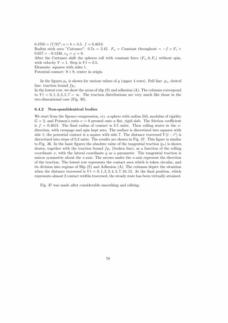
0.4705 = (7/9)3; a = b = 3.5. f = 0.4013.Radius stick area ”Cattaneo”: 0.7a = 2.45. Fx = Constant throughout = −f × Fz ×0.657 = −0.1240, υy = ϕ = 0.After the Cattaneo shift the spheres roll with constant force (Fx, 0, Fz) without spin,with velocity V = 1. Step is V t = 0.5.Elements: squares with sides 1.Potential contact: 9× 9, center in origin.

In the figures px is shown for various values of y (upper 4 rows). Full line: px, dottedline: traction bound fpz.In the lowest row, we show the areas of slip (S) and adhesion (A). The columns correspondto V t = 0, 1, 3, 3, 5, 7 = ∞. The traction distributions are very much like those in thetwo-dimensional case (Fig. 30).

6.4.2 Non-quasiidentical bodies

We start from the Spence compression, viz. a sphere with radius 243, modulus of rigidityG = 2, and Poisson’s ratio ν = 0 pressed onto a flat, rigid slab. The friction coefficientis f = 0.4013. The final radius of contact is 3.5 units. Then rolling starts in the x-direction, with creepage and spin kept zero. The surface is discretized into squares withside 1; the potential contact is a square with side 7. The distance traversed V (t − t′) isdiscretized into steps of 0.2 units. The results are shown in Fig. 37. This figure is similarto Fig. 36. In the basic figures the absolute value of the tangential traction |pτ | is showndrawn, together with the traction bound fpz (broken line), as a function of the rollingcoordinate x, with the lateral coordinate y as a parameter. The tangential traction ismirror symmetric about the x-axis. The arrows under the x-axis represent the directionof the traction. The lowest row represents the contact area which is taken circular, andits division into regions of Slip (S) and Adhesion (A). The columns depict the situationwhen the distance traversed is V t = 0, 1, 2, 3, 4, 5, 7, 10, 13. At the final position, whichrepresents almost 2 contact widths traversed, the steady state has been virtually attained.

Fig. 37 was made after considerable smoothing and editing.

78

Figure 34: Contact stresses in quasiidentical steady state rolling with circular contactarea. (Source: Kalker [12])

79

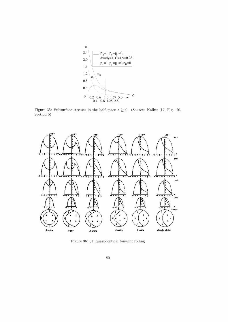
0.4

0.8

1.2

1.6

2.0

2.4

σ

0.20.4

0.60.8

1.01.25

1.6702.5

5.0 8 Z

σI

p =1, p =p =0,dx=dy=1, G=1, ν=0.28

x y

p =1, p =p =0, σ =0x y

z

z ii

−σii

Figure 35: Subsurface stresses in the half-space z ≥ 0. (Source: Kalker [12] Fig. 20,Section 5)

Figure 36: 3D quasiidentical tansient rolling

80

Figure 37: 3D non-quasiidentical transient rolling

81

7 Further and alternate research

1. The work of Bufler [5].In this work, Bufler solves the non-quasi-identical problem of two 2-D bodies rollingover each other with infinite friction (or infinitesimal creepage). An analytical,closed form solution is found.

2. The works of Bentall and Johnson ([2] and [3]).The work from 1967 considers two non-quasi-identical 2-D cylinders rolling overeach other with finite creepage. This work is, in content, a generalisation of Bufler’swork (see 1.). The method is a boundary element method in which the tractionelements are continuous and piecewise linear. The work from 1968 concerns a stripbetween two rolling cylinders. Here also, the traction elements are continuous andpiecewise linear. The solutions are numerical with a partly heuristic algorithm.

3. The work of Braat, Kalker and Saes.This work was published by Kalker[13] and Braat and Kalker [4]. It concerns rollingbodies consisting of different flat layers which are glued together. The geometry is2-D. Examples are: Rubber on steel, steel on aluminium, various kinds of plasticglued onto each other, etc. The rolling bodies are cylinders which are approximatedby layered half-spaces (2-D). Only steady-state rolling is considered, but the layersmay be elastic or viscoeleastic.The solution is found by the boundary element method and the CONTACT algo-rithm. The Panagiotopoulos method is used throughout, as the rolling bodies arenot symmetric. The element equations are found with the aid of an Airy functionH(x, z) which must satisfy a bipotential equation

H,xxxx + 2H,xxzz +H,zzzz = 0

where x is the coordinate in rolling direction and the axis of z points verticallyinto the upper cylinder. The displacements and the stresses are derivatives of Hwith respect to x and z. A Fourier transform is performed in the x-direction, andthe bipotential equation reduces to an ordinary differential eauation in z which canbe solved. Inverse transformation then yields the element equations, which can beinserted into the CONTACT algorithm.

4. The work of Gross-Thebing [8].This work concerns the linear theory of rolling contact when the bodies are 3-D and the creepage is a harmonic function of the time and friction is infinite.Consequently, the tangential contact force is likewise harmonic, but the creepageand the force are not in phase. The theory will be covered extensively in a lectureby Knothe during this course.

5. Kalker’s thesis work [10].This concerns 3-D rolling bodies, quasi-identical, and with an elliptic Hertzian con-tact area. As distinct from the works considered up to now, it is not a boundary

82

element method with rectangular elements which carry a constant or continuous,piecewise linear load, but inside the contact ellipse the displacements are polynomi-als; it can then be shown that the tractions which vanish outside the contact ellipseare polynomials of the same degree as the displacements, but multiplied with acertain function. This is applied to find the connection between the creepage andspin on the one hand and the total force and the twisting moment on the otherhand (creepage-force law) for infinite friction, or in other terms infinitesimal creep-age and spin. It is also applied to find an approximate creepage-force law for finitecreepage and spin, but the process involved does not always converge.

6. Nielsen’s thesis work [15].This concerns 2-D rolling bodies, quasi-identical, with a contact area in the form ofone or more strips. It is a generalisation of Kalker’s work, see 5. The importanceof the work lies in the applications: apart from Carter’s work and an elementarygeneralisation of it Nielsen treats corrugation (among other things the growth ordiminishing of a corrugation field by abrasive wear), velocity dependent coefficientof friction, asperity fields (in which we have multiple contacts), and non-steady 2-Dcontact.

7. The strip theory (Haines/Ollerton [9]).The work of Carter [6] and Nielsen [?] may also be applied as a strip theory, in which2-D solutions are placed beside one another to form a 3-D approximate solution.The idea to do this is due to Haines and Ollerton, who did experiments to verifytheir theory. The work of Nielsen and Haines/ Ollerton is confined to longitudinalcreepage. Kalker [10] extended the work of Haines and Ollerton to lateral creepageand spin. Notably the spin solution is approximate. Note that the simplified theory,treated in Section 3, is also a strip theory.

8. Kalker and Piotrowski [14] investigated the case that the friction coefficient hastwo values, viz. f = fkin when there is slip, and f = fstat when there is no slip.Fastsim was used. The effect on the total tangential force appeared to be small(f = fkin).

References of Section 6

[1] N. Ahmadi (1982), Non-Hertzian normal and tangential loading of elastic bodiesin contact. Ph.D Thesis, Appendix C2. Northwestern University, Evanston IL, USA.

[2] R.H. Bentall, K.L. Johnson (1967), Slip in the rolling contact of two dissimilarelastic cylinders. International Journal of Mechanical Sciences 9, p. 389-404.

[3] R.H. Bentall, K.L. Johnson (1968), An elastic strip in plane rolling contact.International Journal of Mechanical Sciences 10, p. 637.

[4] G.F.M. Braat, J.J. Kalker (1993), Theoretical and experimental analysis ofthe rolling contact between two cylinders coated with multilayered viscoelastic rub-

83

ber, in: A.H. Aliabadi and C.A. Brebbia (Eds.) Contact Mechanics, ComputationalTechniques; Contact Mechanics Publications, pp. 119-126.

[5] H. Bufler (1959), Zur Theorie der rollenden Reibung. Ingenieur Archiv 27, p.137.

[6] F.C. Carter (1926), On the action of a locomotive driving wheel. Proceedings ofthe Royal Society of London, A112, p. 151-157.

[7] H. Fromm (1927), Berechnung des Schlupfes beim Rollen deformierbarer Scheiben.Zeitschrift fur angewandte Mathematik und Mechanik 7, p. 27-58.

[8] A. Gross-Thebing (1992), Lineare Modellierung des instationaren Rollkontaktesvon Rad und Schiene. Fortschritt Berichte VDI, Reihe 12, Nr. 199, VDI-Verlag,Dusseldorf.

[9] D.J. Haines, E. Ollerton (1963), Contact stresses in flat elliptical contact sur-faces which support radial and shearing forces during rolling. Proceedings of theInstitute of Mechanical Engineering Science, 179, Part 3.

[10] J.J. Kalker (1967), On the rolling contact of two elastic bodies in the presence ofdry friction. Thesis Delft.

[11] J.J. Kalker (1971), A minimum principle of the law of dry friction with appli-cation to elastic cylinders in rolling contact. Journal of Applied Mechanics, 38, p.875-880, 881-887.

[12] J.J. Kalker (1990), Three-dimensional elastic bodies in rolling contact. KluwerAcademic Publishers (Dordrecht) 314+XXVI pp.

[13] J.J. Kalker (1991), Viscoelastic multilayered cylinders rolling with dry friction.Journal of Applied Mechanics, 58 p. 666-679.

[14] J.J. Kalker, J. Piotrowski (1989), Some new results in rolling contact. VihicleSystem Dynamics 18, p. 223-242.

[15] J.B. Nielsen (1998), New developments in the theory of wheel/rail contact me-chanics. Thesis Lyngby IMM-PHD-1998-51.

[16] D.A. Spence (1975), The Hertz problem with finite friction. Journal of Elasticity,5, p. 297-319.

84