NASA-CR-201481

JOINT INSTITUTE FOR AERONAUTICS AND ACOUSTICS

/i

Stanford University

National Aeronautics and

Space Administration

Ames Research CenterJIAA TR 113

ROLL-YAW CONTROL AT HIGH ANGLEOF ATTACK BY FOREBODY

TANGENTIAL BLOWING

N. Pedreiro, S. M. Rock, Z. Z. Celikand L. Roberts

Department of Aeronautics and Astronautics

Stanford University

Stanford, CA 94305

October 1995

https://ntrs.nasa.gov/search.jsp?R=19960038364 2018-11-11T12:17:01+00:00Z

Abstract

The feasibility of using forebody tangential blowing to control the roll-yaw motion of a wind

tunnel model is experimentally demonstrated. An unsteady model of the aerodynamics is

developed based on the fundamental physics of the flow. Data from dynamic experiments is used

to validate the aerodynamic model. A unique apparatus is designed and built that allows the wind

tunnel model two degrees of freedom, roll and yaw. Dynamic experiments conducted at 45

degrees angle of attack reveal the system to be unstable. The natural motion is divergent. The

aerodynamic model is incorporated into the equations of motion of the system and used for the

design of closed loop control laws that make the system stable. These laws are proven through

dynamic experiments in the wind tunnel using blowing as the only actuator. It is shown that

asymmetric blowing is a highly non-linear effector that can be linearized by superimposing

symmetric blowing. The effects of forebody tangential blowing and roll and yaw angles on the

flow structure are determined through flow visualization experiments. The transient response of

roll and yaw moments to a step input blowing are determined. Differences on the roll and yaw

moment dependence on blowing are explained based on the physics of the phenomena.

Contents

Abstract

Contents

List of Symbols

List of Figures

2

3

4

5

Introduction

Experimental Apparatus

Wind Tunnel and Model

Model Support System

Air Injection System

Instrumentation and Data Acquisition

Experimental Results

Flow Visualization

Static Aerodynamic Loads

Dynamic Experiments

Equations of Motion

Closed Loop Control

Conclusions

6

7

7

8

10

11

12

12

13

16

17

21

24

Acknowledgments

References

25

25

'fl,ig_QLS_ zg

b

C.

D

I^, I.=

L

lhj

wing span

rolling moment coefficient, M,/q.S,.,b

yaw moment coefficient, M/q.S,_b

jet momentum coefficient, riajVj / q..S_

diameter of fuselage

inertia of the suspension system

model moments of inertia in body frame

inertia of the model about y-axis

axial distance from tip of the forebody

jet mass flow rate

M,, M, rolling moment

z

P

p,q,r

q..

S.t

U

xyz

Y

P

yaw moment

moment about y-axis

intersection of O-axis and y-axis

roll, pitch and yaw rates respectively

dynamic pressure, pU2/2

reference area, wing planform area

freestream velocity

body reference frame, centered at P

first degree of freedom, roll

second degree of freedom

air density

4

List of Figures

Figure 1:

Figure 2:

Figure 3:

Figure 4:

Figure 5:

Figure 6:

Figure 7:

Figure 8:

Figure9:

Figure 10:

Figure 11:

Figure12:

Figure 13:

Figure 14:

Wind Tunnel Model and Detail of Blowing Slots 7

Side View of Test Section and Two Degrees of Freedom Model Support System 8

Block Diagram of Active Cancellation Loop 10

Smoke Flow Visualization Results - _--'t=0, no blowing is applied 12

Smoke Flow Visualization Results - Symmetric Blowing, t_--T=0, C_.0075 13

Roll Angle Effect on Roll and Yaw Moment Coefficients, C, and C,, for T:0 14

Effect of 7 Angle on Roll and Yaw Moment Coefficients, C, and C., for _=0 14

Effect of Asymmetric Blowing on Roll and Yaw Moment Coefficients, 15

Ct and C, for ?:0

Effect of Symmetric Plus Asymmetric Blowing on Roll and Yaw Moment

Coefficients for C_svM=0.01 and T=0 16

Natural Motion of the Two Degrees of Freedom System.

Experiment and Simulation 17

Structure of the Aerodynamic Model. M1Asand M2"s represent static

roll and yaw moments 19

C, and C. response to Step Input Command in C_,. AC, and AC. are usedto indicate variation from the initial value 20

Characteristic of C_ and C. versus AC_ 22

Closed Loop Control of the Two Degrees of Freedom System. Response

to Initial Condition. Asymmetric Blowing 24

Introduction

Advantages of flight at high angles of attack include increased maneuverability and increased lift

during take-off and landing. At these flight conditions the aerodynamics of the vehicle are

dominated by separated flow, vortex shedding and possibly vortex breakdown. These phenomena

severely compromise the effectiveness of conventional control surfaces. Alternate means to

control the vehicle at these flight regimes are therefore necessary. Several methods of active flow

control have been proposed to provide this increased control 1_.

The present work investigates the augmentation of aircraft flight control system by the injection

of a thin sheet of air tangentially to the forebody of the vehicle. This method, known as Forebody

Tangential Blowing (FTB), is proposed as an effective means of increasing the controllability of

aircraft at high angles of attack 5-'. The idea is based on the fact that a small amount of air is

sufficient to change the separation line on the forebody. As a consequence the strength and

position of the vortices are altered causing a change on the aerodynamic loads. Celik 5 has shown

that using this method side force, roll and yaw moments can be generated for angles of attack

from 20 to 50 degrees.

Experimental investigation is conducted to demonstrate the feasibility of using FTB to control

the roll-yaw motion of a wind tunnel model. The model consists of a delta wing-body

combination equipped with forebody slots through which blowing is applied. Experiments are

conducted at a nominal incidence angle of 45 degrees

A unique apparatus that allows the model two degrees of freedom, roll and yaw, is designed and

built. The apparatus is used in dynamic experiments which show that the system is unstable, its

natural motion divergent. External effects of the model support system are actively canceled.

Flow visualization results revealed the vortical structure of the flow to be asymmetric even for

the model at zero roll and yaw angles. The effects of blowing, roll and yaw angles on the flow

structure are determined. Transient response of roll and yaw moments to step input blowing are

characterized in terms of time constants. Differences on the roll and yaw moment behavior due to

blowing are explained based on the physical mechanisms through which these loads are

generated.

A modelfor theunsteadyaerodynamicloadsis formulatedbasedon thebasicphysicsof the

flow. Parametersof theaerodynamicmodelareobtainedfromstaticanddynamicexperiments.

Theaerodynamicmodelcompletestheequationsof motionof thesystemwhichareusedfor the

designof controllawsusingblowingastheonly actuator.Theclosedloopcontrolsystemis

stableasisexperimentallydemonstratedin thewindtunnel.

Experimental Apparatus

W(nd Tunnel and Model:

The wind tunnel facilities of the Aeronautics and Astronautics Depamnent at Stanford University

are used for the experiments. It consists of a closed circuit low speed wind tunnel with 0.45m x

0.45m test section. The maximum test section velocity is 50 m/s.

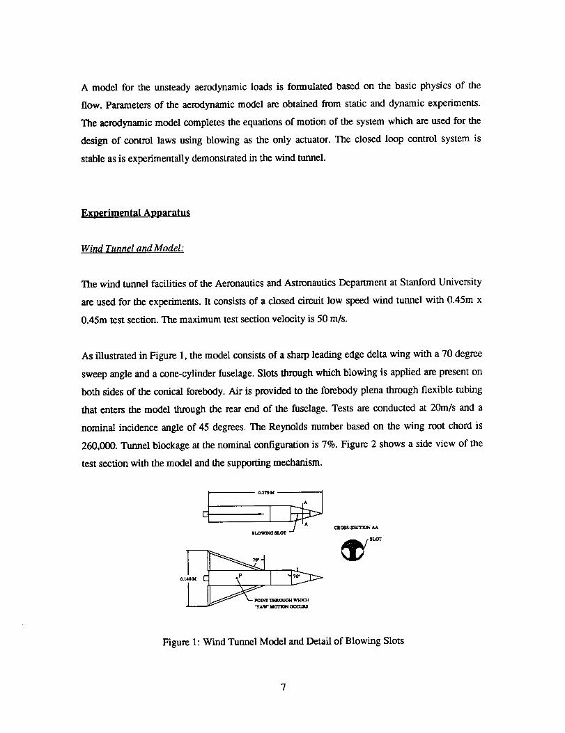
As illustrated in Figure 1, the model consists of a sharp leading edge delta wing with a 70 degree

sweep angle and a cone-cylinder fuselage. Slots through which blowing is applied are present on

both sides of the conical forebody. Air is provided to the forebody plena through flexible tubing

that enters the model through the rear end of the fuselage. Tests are conducted at 20m/s and a

nominal incidence angle of 45 degrees. The Reynolds number based on the wing root chord is

260,000. Tunnel blockage at the nominal configuration is 7%. Figure 2 shows a side view of the

test section with the model and the supporting mechanism.

0.140 M *P 70" 76"

Figure 1: Wind Tunnel Model and Detail of Blowing Slots

Model Support System:

A unique support system is designed and built to implement two degrees of freedom in the

model'*. The objective is to approximate the lateral-directional dynamics of an aircraft. Of

particular interest is the roll-yaw coupling at high angle of attack. The apparatus can be divided

into two subsystems: The first one implements the roll degree of freedom, dp, and consists of a

shaft mounted on bearings. The wind tunnel model is attached to the roll shaft allowing the

model to rotate about its longitudinal axis. The roll subsystem is mounted on a mechanical arm

that can rotate about an axis perpendicular to the models longitudinal axis (Figure 2). The

mechanical arm implements the second degree of freedom, y, and is called the 'yaw' subsystem.

For small roll angles, _/ equals the yaw rate. This approximation can be represented by relating

d:and _, to the roll, pitch and yaw rates, p, q and r respectively.

p = ¢ q = _/sin ¢ r = _cos¢ (1)

Mechanical constraints limit the degrees of freedom as follows: 10l < 105 ° and I': < 30 °.

An important aspect in the design of the experimental apparatus is that the dynamic properties of

the support system should not dominate the dynamic response of the model. Experiments

indicated that the friction in the bearings and the effect of the pressurized tubing are small when

compared with the aerodynamic loads acting on the model'.

MOOKL _ VWIND _ _0_ _iO p1,OW

! I

Figure 2: Side View of Test Section and Two Degrees of Freedom Model Support System

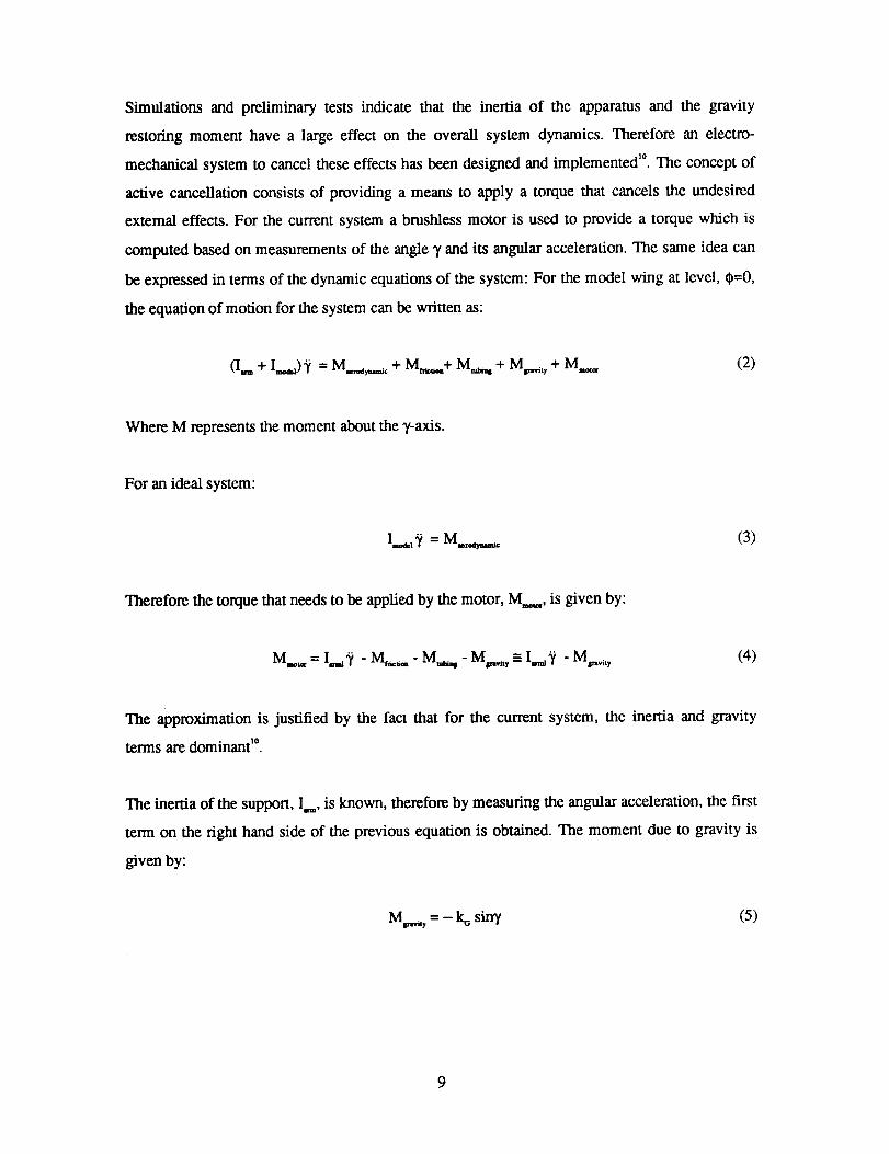
Simulations and preliminary tests indicate that the inertia of the apparatus and the gravity

restoring moment have a large effect on the overall system dynamics. Therefore an electro-

mechanical system to cancel these effects has been designed and implemented TM. The concept of

active cancellation consists of providing a means to apply a torque that cancels the undesired

external effects. For the current system a brushless motor is used to provide a torque which is

computed based on measurements of the angle y and its angular acceleration. The same idea can

be expressed in terms of the dynamic equations of the system: For the model wing at level, ¢=0,

the equation of motion for the system can be written as:

(I + I..._)_ = M..._,.,., + M_,..+ M,_** + M,,.._,y+ M.._, (2)

Where M represents the moment about the y-axis.

For an ideal system:

i d,la? = M,,_r_,_ (3)

Therefore the torque that needs to be applied by the motor, M._,, is given by:

M... = I,_ _ - M_._.. - M_.., - Mv._, = I,,,. _ - M,_,y (4)

The approximation is justified by the fact that for the current system, the inertia and gravity

terms are dominant _0.

The inertia of the support, I, is known, therefore by measuring the angular acceleration, the first

term on the right hand side of the previous equation is obtained. The moment due to gravity is

given by:

Mv_, , = - ko siny (5)

9

Theconstant1%is a knownquantitygivenby theproductof themassof thesupportby the

distanceof its centerof gravityto theT-axis.Theangle7 is measureddirectly.In this waythe

torquethatthemotorshouldapplyatanymomentcanbecomputedfromthesemeasurements.

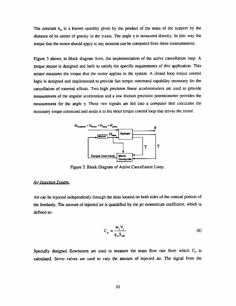
Figure3 shows,in blockdiagramform,the implementationof the active cancellation loop. A

torque sensor is designed and built to satisfy the specific requirements of this application. This

sensor measures the torque that the motor applies to the system. A closed loop torque control

logic is designed and implemented to provide fast torque command capability necessary for the

cancellation of external effects. Two high precision linear accelerometers are used to provide

measurement of the angular acceleration and a low friction precision potentiometer provides the

measurement for the angle T. These two signals are fed into a computer that calculates the

necessary torque command and sends it to the inner torque control loop that drives the motor.

M,.,t_,_ + IV_ + _ +M_

Torque Command Micro

+El

Figure 3: Block Diagram of Active Cancellation Loop.

Air ln_iection System:

Air can be injected independently through the slots located on both sides of the conical portion of

the forebody. The amount of injected air is quantified by the jet momentum coefficient, which is

defined as:

mjvjC_ -_ (6)

q=S_a

Specially designed flowmeters are used to measure the mass flow rate from which C_ is

calculated. Servo valves are used to vary the amount of injected air. The signal from the

10

flowmetersis readinto a computerthat implementsa closedloop logic for C_controlby

commandingtheservovalves.

in_tr_mcntation and Data Acquisition:

The two degrees of freedom, _ and ? are measured by low-friction precision potentiometers. A

six-component force-torque sensor connects the model to the roll shaft and is used to provide

both static and dynamic measurements of the aerodynamic loads. Flowmeters measure the

amount of blowing through each plenum. Two linear accelerometers are mounted to the ?-axle.

Their signals are combined to measure angular acceleration. A torque sensor connects the

brushless motor to the ?-axle and therefore provides a measurement of the torque that the motor

applies to the system.

For the flow visualization experiments, an argon-ion laser and an optical system are used to

generate a laser sheet that is perpendicular to the model longitudinal axis. The optics is mounted

on traversing system located on top of the test section allowing the laser sheet to be moved over

the full length of the model. This capability is used in performing axial scans starting from the

forebody and moving downstream to characterize the development of the flow structure. A

smoke generator located upstream of the model is used to seed the flow. A video camera is

located outside the test section aligned with the model longitudinal axis. The camera is used to

record the results of the flow visualization and also the motion of the model during dynamic

experiments.

Three micro computers equipped with data acquisition boards are used in the experiments. One

computer is dedicated to the active cancellation loop. A second computer is used to implement

the closed loop control of the vehicle, i.e. to control the amount of air injected in each plenum. A

third computer is used for data acquisition.

11

Experimental Results

Flow Visualization:

These experiments reveal the basic structure of the flow. Although four main vortices are

expected, two from the forebody and two from the wing leading edges, experiments demonstrate

that in general only three separate vortical structures can be clearly identified even for a

symmetric condition in which _--y:0 and no blowing is applied (Figure 4b).

By performing axial scans with the laser sheet it is observed that the asymmetry starts early on

the forebody, i.e. close to the tip of the cone, and scales up over the entire forebody TM. As a result

of the asymmetry one vortex will be close to the fuselage and the other will be displaced and

further away as shown in Figure 4a. For the sections where the wing is present, it is observed that

a vortex is formed close to the wing on the same side where the forebody vortex is far from the

fuselage. For the side where the forebody vortex is close to the fuselage no wing vortex is clearly

identified. A possible explanation is given for these observations: Because the forebody vortex is

away from the fuselage and consequently away from the wing the wing vortex develops without

much influence from the fuselage vortex. For the opposite side where the fuselage vortex is very

close to the forebody the wing vortex basically merges with the forebody vortex and therefore a

distinct wing vortex is not observed.

(4a) Station 1 - Forebody - L/D=3 (4b) Station 2 - Wing-Body - L/D=-5

Figure 4: Smoke Flow Visualization Results - _---y=0, no blowing is applied.

12

Theeffectof asymmetricblowing,i.e.blowingappliedfromonesideonly,is mainlyto increase

theasymmetryor invertit dependingonwhichsidetheblowingis applied.Blowingmovesthe

separationlineontheforebodyandcancauseachangein theamountof vorticitythatis shed.As

a consequencethestrengthandpositionsof thevorticesareaffectedby blowing.Experiments

haveshownthat thereis a fmite amountof blowingthat needsto be appliedto invert the

asymmetryof theflow, for the current model configuration at q_-_0 this value is C_ --_-0.0045.

The application of symmetric blowing has the effect of changing the flow structure to a more

symmetric one (Figure 5). For high values of symmetric blowing the flow can be considered

attached on the forebody and its structure is very symmetric even on stations where the wing is

present.

(5a) Station 1 - Forebody - L/D=3 (5b) Station 2 - Wing-Body - L/D=-5

Figure 5: Smoke Flow Visualization Results - Symmetric Blowing, _--y=0, C_=.0075

Experiments show that the asymmetric structure can change significantly by a change in the roll

angle. The flow structure is not as sensitive to a change in "r.

Static Aerodynamic Loads:

Static measurements for the roll and yaw moment as a function of _, 7 and C, are presented in

Figures 6 through 8. A convention is adopted that right side, i.e. starboard blowing is positive

and left side, i.e. port side blowing negative. In Figure 6 the effect of the roll angle on C_ and C,

is shown for y=0 and various C_. The C, curve for C_=0 presents a change in slope for __-15 °.

13

ForC_=.02achangeoccursat (_-_--5°. Also for C_=0 the C, curve presents a large change in slope

for tp<-15°. The fact that these changes are not symmetric, i.e. they only occur for _<0, indicates

that they are caused by geometrical imperfections on the tip of the conical forebody.

el

0.05

0.04

0.03

0.02

0.01

0

-0.01

-0.02

-0.03

-0.04

-0.05-40

. . -_ ° ° °, - - _ - .

, .uz, , .

I 8 I I I I I

-30 -20 -tO 0 10 20 30 40

¢ (Deg.)

C_

0.5

0.4

0,3

0.2

0.1

0

-0.1

-O.2

-0.3

-0.4

-0.5

-4O

' ' :-.o2 , : : :

i i i i i i i

-30 -20 -10 0 10 20 30

0 ta_eg.)

Figure 6: Roll Angle Effect on Roll and Yaw Moment Coefficients, C, and C, for y=0.

4O

Figure 7 presents curves for C, and C, versus "yfor _=0 and various C_. Comparing Figures 6 and

7 shows that the slopes of the roll and yaw moment curves are not as sensitive to "t as they are to

¢p.This is in agreement with the flow visualization experiments which indicate the flow structure

to be less dependent on "/than on #.

el

0.06

0.04

', : : .02 : c,=o0.02

0

.0._

-30 -20 -10 0 10 20 30

y (Deg.)

C_

0.4

0.3

0.2

0.1 , , ,

0

-0.1 _

-0.2

.0.'4

,,_.4 .....................

-0.5 , , , ' '

-30 -20 -10 0 10 20 30

_/(Deg.)

Figure 7: Effect ofy Angle on Roll and Yaw Moment Coefficients, C, and C., for #=0.

The effect of asymmetric blowing on C_ and C, is shown in Figure 8 for "y=0 and various _. In

this case blowing is applied either on the right or left side. As seen the roll moment varies

14

abruptlyfor IC_I<0.01andtheyawmomentpresentsalargevariationfor0.01<C_,<0.Degani'has

shownthatsmallamountof blowinghasaneffectsimilarto thegeometricimperfectionsnearthe

tip oftheforebodyandcancauseflowinstabilitiesthatleadto asymmetryin theflow.Thisis the

mostplausibleexplanationfor theroll momentbehaviorshowninFigure8.ForIC_I<0.01theroll

momentis moresensitiveto changesin C_,thantheyawmoment.Thisfactcanbeexplainedby

thedifferentphysicalmechanismsthroughwhicheachof theseloadsaregenerated.ForIC_l<0.01

thecontributionsof thedirectjet momentumto C,andC, arenegligible.In thiscase,it canbe

consideredthat the roll momentis only generatedat stationswherethe wingsarepresent.

Becausethefuselageis of circularcross-section.Thereforetheroll momentis determinedby the

flow overthewingswhichmightbesubjectto largeinstabilitiesasvortexbreakdown.Theyaw

momentisdeterminedbythepressuredistributionoverthefuselage.Thewingsdonotcontribute

to C.becausetheyarethinandonlyofferareaperpendicularto theyawaxis.Theflow overthe

forebodyhasagreatereffecton theyawmomentdueto its distanceto thecenterof massof the

model.Forstationsontheforebodyit is expectedthatflow instabilitiesarenot fully grownand

arethereforelessimportantfortheyawmoment.

Cl

0.04

0.03

0.02

0.01

0

-0.01

-0.02

-0.03

•0.04 , , ,-0.0e -0.o6 -0.o4 -o.o2

, _i0 *¸. . 'o . .'.. ' ...... 'o . ' .....

..i ....... " :.!..

iI iili

i i i i

0 0.02 0.04 0.06 0.06

C_

C_

0.6

0.4

0.2

0

-0.2

-0A

-0.6

-0.08

-I0 o

i i i i i i a

-0.06 -0.04 -0.02 0 0.02 0.04 0.06 0.08

C_

Figure 8: Effect of Asymmetric Blowing on Roll and Yaw Moment Coefficients,

C, and C,, for 7"=0.

Figure 9 shows the result of applying symmetric and incremental asymmetric blowing on the roll

and yaw moment coefficients. An equal amount of blowing, C_._.,,, is applied on both sides and

additional asymmetric blowing, AC_, is applied either to the right or the left side. As seen the

major effect consists in producing a linear characteristic and eliminating the sudden variations

15

thatoccurin theasymmetricblowingcase.Thesymmetryobserved in these plots agrees with the

symmetric flow structure obtained from the flow visualization experiments (Figure 5).

O.OS ....... 0.5 ; : ; ; ; ; ;

o.o, '_ ', : ', : J _-_ o.,

....... ol,ii io.o3--,_- -:- --:- - -: ...... _,:o 0.2o.o_ : : : ' ' , lo*

ooii!i i!io1! i!!Cl o " " ' ' , 12o° C= o

_.oI -o._ "2°°i ' ' " :

•0.02 41.2

-0.0_ -0.3

-0.04 -0.4

-0.5 , , ' ' '-0.05 , , , ' ' ' '.-O.OB -0,06 -0.04 -0.0_ 0 0.02 0.04 0.06 0.08 -0.08 ..0.06 -0,04 -0.02 0 0.02 0.04. 0.06 0.08

AC_ AC_

Figure 9: Effect of Symmetric Plus Asymmetric Blowing on Roll and Yaw Moment

Coefficients for C_,,M=0.01 and y=0.

Dynamic Experiments:

The results for the static roll and yaw moment show that these moments are not zero for _--q,=0

and C_--0. Also the positive slope of the curve (2. versus y indicates that the system is statically

unstable at this condition. An experiment is performed to determine the dynamic characteristics

of the system since those cannot be inferred from the static data alone: With no blowing applied

the model is released from a certain initial condition. This represents the natural motion of the

system and will ultimately determine if the system is stable or unstable. Figure 10 shows the time

histories for _ and Y when the model is released from ___, also shown are the results from

simulations using the aerodynamic model described in the following section. As seen, the system

is unstable. The motion is divergent and is stopped when the system approaches the mechanical

limit of y.

16

16

O14 . . . '.... ' .... ' .... '... _' _ .0

', :12 ---: .... :.... ,,.... :---_/-,o ............. :.... :- - -o_ - .

', : , , o,

_(Dcg') 6 _ii42q8 - - - ,.... , .... , .... , - "O ; " - "

i i i i i

0 0.1 0.2 0.3 0.4 0.5 0.6

Time (s)

7(Deg.)

20

15

I0

...!.... i.... i...., , SIMULATION -__ -/0 u

f_iii" . . ',,.... ',,.... ,,,.... ,,., _o_,. . _

0 0.1 0.2 0.3 0.4 0.5 0.6

Time (s)

Figure 10: Natural Motion of the Two Degrees of Freedom System. Experiment and Simulation.

Equations of Motion

In order to study the dynamic characteristics of the system it is necessary obtain its equations of

motion. For the two degrees of freedom system those are:

I MR_ + sin _ COS_b(IMz -- I My )'Y2+ COS01Mxz_ = M1

(I A + IMy sin 2 _ + IM z COS 2 ¢_);_ + 2COs_sine_(IMy - IMz )_ + (_cos¢_ -- ¢_2 sin_)iM, _ = M2(7)

For the current model configuration, where a vertical stabilizer is not present the product of

inertia is zero.

M, is the moment about the model longitudinal axis,. M 2 is the moment about the T-axis. M_ and

M 2 are given by:

A T F

M,=M 1 +M 1 +M 1

M =M2^+IV_T+M_ ' +M2°+M2" (8)

Where the superscripts indicates the origin of the moments:

17

A = aerodynamicsT = airsupplytubingF = frictionof beatingsandpotentiometerG= gravityrestoringmomentM = motor

For I@1< 40 ° the moment caused by to the air supply tubing on the first of equations (8) is

negligible 10.The torque applied by the motor is given by:

M T O

M2 =-M 2 -M_ +I,'_ (9)

The moments caused by friction of the bearings and potentiometers can be written as:

p F

M1 =-C F_ M 2 =-D FY (10)

C Fand DF are determined experimentally.

Substituting expressions (9) and (10) in equation (8):

(11)

Expressions for the aerodynamic moments M, ^ and M2^ are necessary to complete the above

equations. Wong 3 developed an aerodynamic model for a delta wing undergoing roll oscillations

that assumed that the dynamic loads could be approximated by lagged static loads and a pre-

specified function of the roll rate. This basic idea is extended by including damping effects

proportional to roll and yaw rates, cross-coupling terms in roll and yaw and apparent mass effects

due to angular acceleration. The lag in the static loads is justified by comparing static and

dynamic flow visualization results which clearly show that the vortex dynamic position lags with

respect to the static one'. It is known that the strength of the shedding vortices is also affected by

the motion of the vehicle. The current approach lumps position and strength effects by lagging

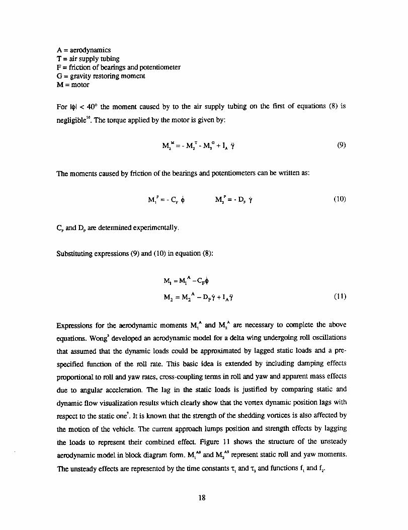
the loads to represent their combined effect. Figure 11 shows the structure of the unsteady

aerodynamic model in block diagram form. M_"s and M_"s represent static roll and yaw moments.

The unsteady effects are represented by the time constants x, and _2and functions f_ and f2.

18

.I 1 I

_P'_; ' fl = f,(_),_/,_)f2=

'L

Figure 11: Structure of the Aerodynamic Model. M1"s and M2Asrepresent static

roll and yaw moments.

Functions fl and 1'2are assumed linear in the angular rates and accelerations:

f_ = c_ + c,_, +c_

f2 = D,_ + D_,_,+ D_:¢ (12)

Given the structure shown in Figure 11 and the expressions for f, and f2, the equations for the

aerodynamic moments M, ^ and M2^ are:

M1A = _I +_1 +C_+C'i,"i'+C_;_

M2 A = )"2 + _2 + D$_b + D.t' i' + D,y'_ (13)

_t and _2 are the lagged static mU and yaw moments for C:O, and are given by the following

equations:

(14)

4, and _ represent the effect of blowing on the roll and yaw moment and are given by:

19

(15)

Where x) and x,r are time constants that characterize the roll and yaw moment response to a

variation in blowing, ACw They include the effect of valve and plenum dynamics as well as the

time it takes for the change in the flow structure to affect the moments. Figure 12 shows the

response of Ca and C. for a step input command in C_,. Also shown are the results of the

parameter fitting using equations (15).

ACl

o.o, : : .-.: :

0.03_

°°r....,, . . .,2

-0.01

0 0.2 0.4 0.6 0.8

Tune (s)

AC,

0.5

0.4

0.3

0.2

0.1

0

-0.1

..... -:, .,- 7.TM

...... i ................

..... 4 ................

i

i i i i

0.2 0.4 0.6 0.8

Time (s)

Figure 12: Ca and C. response to Step Input Command in Cw ACa and AC, are used toindicate variation from the initial value.

Substituting equations (11) through (15) into (7) the equations of motion for the two degrees of

freedom system are obtained. Dynamic stability derivatives and time constants x_ and x2 are

determined using a minimum least squares fit to the time histories of _ and "gfor a set of dynamic

experiments. Time constants x, and 'h are determined from the rob and yaw moment response to

a step input command in C_, (Figure 12).

The natural motion of the system is shown in Figure 10. Experimental results are compared with

simulation using the aerodynamic model developed. The simulation agrees well with the

measured response.

20

Closed Loop Control

To design a control law that stabilizes the naturally unstable system the equations of motion are

linearized as follows: For small static equilibrium roll and yaw angles, i.e. _ and YE<< 1, _pand 7

are redefined as ¢_-_Eand T-TBand equations (7) and (11) are written as:

AIMzT + DF)' = M 2 (16)

About the static equilibrium position, M1"s and MaA' can be expressed as:

(17)

C,, C r , D, and D r are the static stability derivatives obtained from the curves for the roll and

yaw moments versus _ and "t.

Equations (15) represent the effect of blowing. For the asymmetric blowing case and IC_l <0.01

F, and F, arc highly non-linear functions of C_,, as seen in Figure 8. Furthermore operation in

this region is prone to generating non-robust control laws because C, and C. are very sensitive to

small variations in blowing. Given the above reasons the low blowing intensities are avoided by

employing the following control strategy: A minimum amount of blowing other than zero, C_,

is chosen and additional blowing AC_, is added to that value, i.e.:

C_ _ C_o + ACg (18)

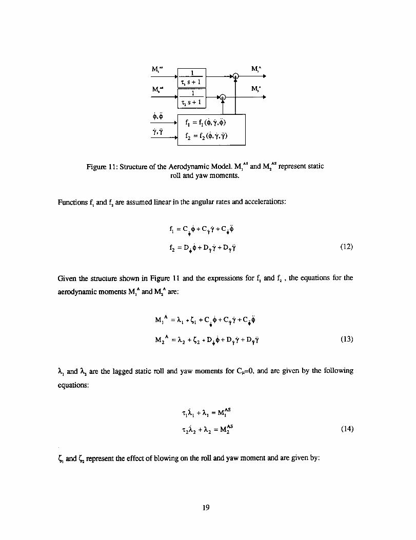
The curves for C, and C versus AC_, have the general form shown in Figure 13.

21

C_orC.

A AC_

Figure 13: Characteristic of C, and C. versus AC_.

A describing function approach is used to determine the equivalent gain of the curves C_ and C.

versus AC_. The actual gain, N(A), depends on the amplitude of the input, A, and is given by:

4DN(A) = m + m (19)

nA

D and m are defined in Figure 13. An average amplitude is selected for AC, and used to calculate

CB and D Bthe equivalent gains for roll and yaw moment respectively. Expressions for F, and F2

ale:

F1 = CBACa. F, = D BACa. (20)

For the symmetric blowing case there is no need to apply the describing function approach

because the C, and C, variation with AC_.is fairly linear (Figure 9).

The lineafized equations of motion are:

(IM_ - C_)_ = (Ct - CF)_ + C?_/+ k I + _I

(IMz -- D,t)_ = (D_ - D F)_' + Dt_ + _'2 + _2

"q_._+ _._ = C,qb + C,¢3'

'_'_2 = -_2 + DBACv" (21)

22

Thesecanbewrittenin theform:

i(t) = Ax(t)+Bu(t) (22)

Wherex is thestatevectorandu thecontrolvariable:

u(0--=AC_ (23)

A control logic is designed using the Linear Quadratic Regulator (LQR) method with weights on

_, _/, #, "_and AC_. The result is a gain matrix, -K, that is multiplied by the state vector x(t) to

generate the required control, i.e.,

u(t) = - Kx(t) (24)

This control law requires knowledge of the state vector. ¢?and _/are measured directly. The other

state variables are obtained from these measurements and the use of an estimator.

The performance of the closed loop system is shown in Figure 14. The plots show data obtained

during a real time closed loop control experiment. In this case the model was released from

_-38 ° and ?_--14°. It is seen that the logic makes the system stable and regulates _ and T to close

to zero. The third plot shows the control effort, C_. Two curves are shown: C_>0 for right side

blowing and C_,<0 for left side blowing.

Similar results are obtained using symmetric and asymmetric blowing. The disadvantage of the

symmetric blowing case is a larger use of air.

23

4O

3O

2O

10

0

-10 . .

-20

0

I I i i i I I

1 2 3 4 5 6 7

Time (s)

15

10

-I0

0

° - . ° - - °. ° - -. ° . - - . - .....

• o ' o

i ....................

8 , i i i i ,

1 2 3 4 5 6 7

Time (s)

0.06

0.04

0.02

-0.02

-0.04

-0.06 i i i , i i ,

1 2 3 4 5 6 7 8

Tune (S)

Figure 14: Closed Loop Control of the Two Degrees of Freedom System. Responseto Initial Condition. Asymmetric Blowing.

Conclusions

The use forebody tangential blowing (FTB) to stabilize the roll-yaw motion of a delta wing-body

model is experimentally demonstrated in the wind tunnel.

An aerodynamic model that is suitable for controls is developed based on: Static measurements

of the aerodynamic loads and basic physical representation of the main dynamic effects. The

model is validated through dynamic experiments and used in the design of closed loop control

laws. The control logic stabilizes the system using blowing as the only actuator. It is shown that

asymmetric blowing is a highly non-linear effector that can be linearized by superimposing

24

symmetricblowing.Thetransientresponseof roll andyawmomentsto astepinputblowingare

determined.

Dynamic experiments are conducted using a unique apparatus that allows a wind tunnel model

two degrees of freedom, roll and yaw. These experiments show that at 45 degrees angle of attack

the natural system is unstable presenting a divergent motion.

The flow structure over the wing-body combination at 45 degrees angle of attack is asymmetric.

As determined from flow visualization experiments. The coupling between forebody vortices and

wing vortices is strong and an asymmetry that starts on the forebody will determine the structure

of the flow downstream. At sections where the wing is present three main vortical structures are

discemible. Asymmetric FTB increases the flow asymmetry or inverts it depending on which

side of the model blowing is applied. The asymmetry can also be inverted by a change in roll

angle. The flow structure is not as sensitive to changes in yaw angle. Differences on the roll and

yaw moment dependence on blowing are explained based on the different mechanisms through

which they are generated.

Acknowled__rnents

This work is supported by the NASA-Stanford Joint Institute for Aeronautics and Acoustics,

NASA Grant NCC 2-55.

References

1. Ericsson, L.E. and Reding, J.P., "Alleviation of Vortex Induced Asymmetric Loads", Journal

of Spacecraft and Rockets, Vol 17, Nov.-Dec. 1980, pp. 546-553.

2. Rao, D. M., Moskovitz, C., and Murri, D. G., "Forebody Vortex Management for Yaw

Control at High Angles of Attack," Journal of Aircraft, Vol. 24, No. 4, p. 248-254, April 1987.

3. Wong, G.S., "Experiments in the Control of Wing Rock at High Angles of Attack Using

Tangential Leading Edge Blowing," Ph.D. Dissertation, Aeronautics Department, Stanford

University, 1991.

25

4.Ng,T.T., and Malcolm, G. N., "Aerodynamic Control Using Forebody Strakes," AIAA Paper91-0618.

5. Celik, Z.Z. and Roberts, L., "Vortical Flow Control on a Wing-Body Combination Using

Tangential Blowing," AIAA Paper 92-4430.

6. Celik, Z.Z., Roberts, L. and Pedreim, N., "The Control of Wing Rock by Forebody Blowing,"

AIAA Paper 93-3685.

7. Celik, Z.Z., Roberts, L. and Pedreiro, N., "Dynamic Roll and Yaw Control by Tangential

Forebody Blowing," AIAA Paper 94-1853.

8. Adams, R. l., Buffington, J. M., and Banda, S. S., "Active Vortex Flow Control for VISTA F-

16 Envelope Expansion," AIAA Paper 94-3681.

9. Degani, D., "Numerical Investigation of the Origin of Vortex Asymmetry," AIAA Paper 90-0593.

10. Pedreiro, N., "Experiments in Aircraft Roll-Yaw Control Using Forebody Tangential

Blowing," Ph.D. Dissertation (to be published), Aeronautics and Astronautics Department,

Stanford University.

26