Ocean Modelling 69 (2013) 136–145

Contents lists available at SciVerse ScienceDirect

Ocean Modelling

journal homepage: www.elsevier .com/locate /ocemod

Roles of shelf slope and wind on upwelling: A case study off east andwest coasts of the US

1463-5003/$ - see front matter � 2013 Elsevier Ltd. All rights reserved.http://dx.doi.org/10.1016/j.ocemod.2013.06.004

⇑ Corresponding author at: State Key Laboratory of Marine EnvironmentalScience, Xiamen University, Xiamen 361005, Fujian, China. Tel.: +86 5922185510; fax: +86 592 2185570.

E-mail address: ywjiang@xmu.edu.cn (Y. Jiang).

Zhaoyun Chen a,d, Xiao-Hai Yan a,b,d, Yuwu Jiang a,d,⇑, Lide Jiang c

a State Key Laboratory of Marine Environmental Science, Xiamen University, Xiamen 361005, Fujian, Chinab Center for Remote Sensing, College of Earth, Ocean and Environment, University of Delaware, Newark, DE 19716, USAc NOAA/NESDIS/STAR, E/RA3, 5200 Auth Road, NOAA Science Center, Camp Springs, MD 20746, USAd Joint Institute for Coastal Research and Management (UD/XMU Joint-CRM), USA

a r t i c l e i n f o a b s t r a c t

Article history:Received 18 January 2013Received in revised form 11 June 2013Accepted 14 June 2013Available online 28 June 2013

Keywords:Upwelling ageUpwelling indexShelf slopeWindSea surface temperatureNumerical model

To understand the differences in upwelling tendency between the east and west coasts of the U.S., ide-alized numerical experiments were performed to examine the upwelling response to wind and shelfslope. The primary results show that steeper slope leads to narrower cross-shore width of surface Ekmandivergence (WSED) and larger vertical velocity, while stronger upwelling favorable wind stress inducesbroader WSED and larger vertical velocity. Meanwhile, the wind duration is substantial to determineboth the area and intensity of upwelling off the coast. The tendencies for cold upwelling areas off eachcoast are compared by the upwelling age, which is defined as the ratio of the duration of upwelling favor-able wind to the advection time. The advection time, defined as the time scale for cold water to beadvected from the pycnocline to the ocean surface, is improved to comprise of climbing time and upwell-ing time. The latter is related to the upwelling divergence driven by surface Ekman flow. The depth of theswitch point of these two processes is approximately 0.9DE (DE is the Ekman depth). The proposed for-mula for the advection time is found to be consistent with estimates derived from the use of particle tra-jectory analysis within the numerical model results. The consideration of upwelling age shows thatdifferences in wind forcing are more important than bottom slope in accounting for the different charac-teristics of upwelling areas off the California and New Jersey coasts.

� 2013 Elsevier Ltd. All rights reserved.

1. Introduction

Upwelling is an important oceanographic phenomenon incoastal ecosystems because the onshore subsurface flow bringsbottom nutrients up into the euphotic zone and leads to high con-centrations of plankton and zooplankton. The development of coldupwelling area consists of two stages: (1) cold water advectedfrom the pycnocline to the surface (the time scale of this processis known as the advection time (Jiang et al., 2012)); and (2) theupwelling front at the sea surface migrating offshore to form alarge area of cold water off the coast. It is found that gentle slopeis unfavorable for the wind-induced upwelling (Allen et al., 1994;Jiang et al., 2011). However, little work has been done (Jianget al., 2012) to compare the upwelling systems off the Californiacoast to those off the New Jersey coast regarding the wind andslope effects on coastal upwelling. Based on Ekman theory, Jianget al. (2012) proposed a concept of ‘‘upwelling age’’, C, which is de-

fined as wind duration, twind, divided by advection time tad, i.e.C = twind/tad. The advection time is the required time to advectthe cold water from pycnocline to the coast, and is inversely pro-portional to wind stress and shelf slope. The advantage of this indi-cator to quantify the coastal upwelling is the multipleconsiderations of the effects of wind duration, shelf slope and windstrength, all of which are crucial factors in determining coastalupwelling tendency. In particular, we focus on the study of advec-tion time, which is the primary part of the upwelling age quantify-ing the tendency for the development of a cold upwelling area, andseek to explain the significant differences that exist between thecold upwelling areas off these two coasts as observed in satellitesea surface temperature (SST) images.

The duration of the upwelling favorable wind plays an impor-tant role in the spatial extent of the upwelling and the amount ofthe temperature drop. The cold upwelling area is closely relatedto the time-integrated wind stress (Breaker and Mooers, 1986;Jiang et al., 2011). When the upwelling favorable wind weakens,the upwelling circulation relaxes, leading to reduced upwellingintensity and weaker alongshore currents (Melton et al., 2009;Pringle and Dever, 2009). In addition to the effects of the wind,the bathymetry and coastal orientation strongly affect the

Z. Chen et al. / Ocean Modelling 69 (2013) 136–145 137

upwelling frequency and intensity off coastal regions (Narimousaand Maxworthy, 1986; Song and Haidvogel, 1993; Torres et al.,2003; Gomez-Gesteira et al., 2008). Rodrigues and Lorenzzetti(2001), Song et al. (2001), and Song and Chao (2004) all suggestedthat it was necessary to combine the effects of wind stress togetherwith bottom slope for studying coastal upwelling systems. Estradeet al. (2008) concluded that a steep shelf favored narrow cross-shore width of surface Ekman divergence (WSED), while a gradualshelf favored broad WSED. A gradual shelf slope concentrates theonshore nutrient transport in the bottom boundary layer, while asteeper shelf slope increases the interior transport between thesurface and bottom boundary layers (Jacox and Edwards, 2011).Further, a poleward alongshore undercurrent will develop onlyover steeply sloped shelves (Choboter et al., 2011).

With respect to the upwelling off the California coast, the SST im-age (Fig. 1(a)) clearly shows that the coastal upwelling, which oftenextends several hundred kilometers from the coast from mid-Marchto mid-October, is the dominant physical process (Breaker and Moo-ers, 1986). By comparison, it is much weaker with a cold band�25 km off the New Jersey coast (Fig. 1(b)), in spite of the fact thatthe dominant wind is upwelling favorable during summer. Theupwelling often stays in stage (1) that subsurface water advects on-shore off New Jersey coast, while upwelling further develops in stage(2) off California coast. The less frequent and less intense upwellingoff New Jersey can be attributed to the higher intermittency of theupwelling-favorable wind (Smith, 1968) and the more gradual shelfslope, both of which are important factors that restrict the strengthof coastal upwelling circulations (Garvine, 2004). The bathymetryoff the New Jersey coast shows that the shelf has roughly an orderof magnitude lower bottom slope than that off the California coast(Clarke and Brink, 1985; Lentz and Trowbridge, 1991; Garvine,2004). Typical bottom slopes off the California coast are�1 � 10�2, whereas the shelf bathymetry off the New Jersey coastis characterized by a more gradual slope �1 � 10�3.

Fig. 2(a) and (b) shows the stick diagrams of wind velocity ob-tained from National Data Buoy Center (NDBC; buoy 46027 and44009, indicated by the black squares in Fig. 1(a) and (b)) off eachcoast. The wind stress is decomposed to alongshore and cross-shore components. The alongshore component direct determiningoffshore Ekman transport is plotted in Fig. 2(c) and (d). Upwellingfavorable winds are prevalent off the California coast with typicalevent durations of approximately one week, while the wind direc-tion shifts back and forth off the New Jersey coast, with the upwell-ing favorable wind events lasting only 2–3 days (Jiang et al., 2012).In addition, the wind is much weaker and more variable in itsdirection off the New Jersey coast than those off the Californiacoast. Since the wind forcing drives the coastal upwelling circula-tion, its strength and duration play dominant roles in determining

Fig. 1. MODIS SST (�C) (a) off the California coast on 25 June, 2003, and (b) off the New Jesquares. Typical shelf slope is a = 10�2 for California, and a = 10�3 for New Jersey.

the spatial extent of cold water. The bottom bathymetry can act toinfluence the upwelling process through the effect of bottom fric-tion. As a result, we address the question of the relative importanceof the wind forcing and the shelf slope in controlling the upwellingcharacteristics off the California and New Jersey coasts. In addition,it is also very important to fully explain the remarkable differencein the responses of these two upwelling systems.

This paper is organized as follows: The idealized numericalmodel is introduced in Section 2. In Section 3, the model is appliedwith spatially uniform wind fields to simulate the coastal upwell-ing processes for several idealized bottom bathymetries. As a con-cept to describe the tendency of cold upwelling areas, the theory ofadvection time is extended to include climbing and upwelling timescales, which are quantified through the use of a Lagrangian parti-cle method within the numerical model. A discussion of the resultsis presented in Section 4, followed by conclusions in Section 5.

2. Numerical model

The numerical model used for the idealized simulations of theupwelling response to different wind and shelf slopes is the Regio-nal Ocean Modeling System (ROMS) model (Shchepetkin andMcWilliams, 2005). ROMS is a three-dimensional, hydrostatic,primitive equation ocean model which uses a stretched, general-ized, terrain-following r coordinate (Song and Haidvogel, 1994)and a horizontal, orthogonal, curvilinear Arakawa C-grid scheme.The model is configured with land on the western boundary, andthe boundary conditions are periodic in the north and south, andoutwardly radiative on the open eastern boundary. The turbulenceclosure scheme used is the Mellor-Yamada level-2.5 (MY-2.5) tur-bulence kinetic energy scheme. A third-order, upstream-biasedhorizontal advection scheme is used for the tracer and momentumequations, and a logarithmic bottom drag is assumed to calculatethe bottom friction. The horizontal model domain is 225 kmcross-shore with 0.5 km resolution, and two grid points in thealongshore direction. The minimum water depth is set to 5 m atthe coast, and the bathymetry gradually descends to 200 m witha constant slope and rapidly drops to 250 m by the outer boundaryto represent the continental slope (Fig. 3). The model is dividedinto 25 vertical terrain-following r-levels, where hs = 3.0, hb = 0.4and hc = 5 m indicate that more grid points are concentrated nearthe surface (Fig. 3). The model uses an f-plane approximation witha Coriolis parameter of f = 10�4 s�1. The initial velocities and sur-face elevation are set to zero, and the temperature is initializedin the whole model domain in the form:

TðzÞ ¼ p2

arctanzþ 17

5

� �þ 20; ð1Þ

rsey coast on 25 August, 2003. Wind measurements from NDBC are marked by black

Fig. 2. Stick diagrams of wind velocity (m s�1) from the NDBC buoys (a) for the California coast, 14–28 June, 2003, and (b) for the New Jersey coast, 14–28 August, 2003.(c) and (d) are the corresponding alongshore components (N m�2). Positive value means an upwelling favorable wind direction.

Fig. 3. Different shelf slopes in the numerical model experiments. Black solid linesdenote r-levels distribution for the case of slope a = 1.0 � 10�3.

138 Z. Chen et al. / Ocean Modelling 69 (2013) 136–145

where z is the depth in meters. The temperature decreases from22 �C at the surface to 20 �C at 17 m depth, and is nearly constant(�17.7 �C) below 50 m depth. The thermocline is located at 17 m.No heat or water mass fluxes are input at the air-sea interface,and the tidal processes are not included in the model. The initiallystationary ocean is forced by spatially-uniform wind blowingfrom south to north, which gradually increases according tos(t) = s0(1 � e�3t), where t is the time in days, s0 is the alongshorewind stress. The wind reaches 95% of s0 in one day. The resultswere used for analysis after the model was run for 10 days.

3. Results

3.1. Model experiment schemes and results

Since the bathymetry and wind conditions are strikingly differ-ent off the east and west coasts of the U.S., the numerical model isrun with different bottom slopes and wind stresses to check theireffects on the wind-driven coastal upwelling system. To examinethe effect of bathymetry, alongshore wind stress s0 is set to

0.05 N m�2, which is typical alongshore wind forcing off the NewJersey coast in summer (Fig. 2(d)), and six cases are run with shelfslopes a = 10.0 � 10�3, 7.5 � 10�3, 5.0 � 10�3, 3.0 � 10�3,2.0 � 10�3, and 1.0 � 10�3 (Fig. 3). To examine the effect of wind,six cases with a constant slope a = 1.0 � 10�3 and different windstresses are run, corresponding to s = 0.01, 0.025, 0.05, 0.1, 0.15and 0.2 N m�2. No cross-shore wind and Ekman pumping effectsare considered in any of the case studies.

Because the parameters of the numerical model are invariablein alongshore direction, and the model is expected to be two-dimensional. Cross-shelf profiles of the cross-shore velocity U, ver-tical velocity W and temperature T on day 10 are presented in Fig. 4with MY-2.5 eddy viscosity profile. Taking the case of wind stresss = 0.05 N m�2, slope a = 1.0 � 10�3 as a reference case (Fig. 4(d)–(f)), the U field shows that the wind-driven, offshore transportoccurs in the upper 20 m of the water column, with the onshorereturn flow mostly occurring in the bottom Ekman boundary layer.The return current interacts with the surface Ekman offshore flowon the inner-shelf within 30 km of the coast. The inner-shelf is de-fined as the transition region where the surface and bottom Ekmanlayers interact (Lentz, 1995). The shallow water effect over the in-ner-shelf causes a decrease of the surface Ekman layer thickness.The offshore current intensifies at 15 km offshore to approximately0.05 m s�1. The onshore return flow is approximately 0.02 m s�1

and 20 m thickness, which translates to an upslope current withlarge vertical velocity near the bottom. The sea surface level islow near the coast, and increases offshore. The sea level changecaused by the surface offshore Ekman transport yields a pressuregradient directed westwards that generates a northward geo-strophic alongshore current (not shown). As a consequence of theonshore return flow, the 20 �C isotherm lifts from the thermocline,and intersects the surface producing an extensive upwelling areanext to the coast. The minimum SST appears at a location of15 km offshore, and the cold water further drifts offshore andmixes with the surface warm water producing an upwelling frontat 30 km off the coast.

An order of magnitude steeper shelf slope (a = 1.0 � 10�2)yields the same magnitude of cross-shore velocity U, but the sea-ward boundary of inner-shelf is closer to the coast (Fig. 4(a)). Out-side of the inner-shelf, the surface and bottom Ekman layers are

Fig. 4. Cross-shore profiles of the cross-shore velocity U (m s�1), vertical velocity W (m s�1) and temperature T (�C) from the numerical model. (a)–(c) for slope a = 10�2, windstress s = 0.05 (N m�2), (d)–(f) for slope a = 10�3, wind stress s = 0.05 (N m�2), (g)–(i) for slope a = 10�3, wind stress s = 0.2 (N m�2).

Fig. 5. Time evolution of offshore positions of the upwelling front in different cases,defined as DT = 2 �C.

Z. Chen et al. / Ocean Modelling 69 (2013) 136–145 139

well separated, and no cross-shore flow is observed between them.In contrast to the cross-shore velocity, the vertical velocity is muchmore sensitive to the shelf slope (Fig. 4(b)). The W is one order ofmagnitude larger, and leads to a narrower band of return currentand the location of the maximum in vertical velocity closer tothe coast. Consequently, colder water is found in the nearshore(Fig. 4(c)).

In the case of stronger wind forcing (s = 0.2 N m�2), the surfacemixed layer thickens to roughly 40 m, and the width of the inner-shelf region is broader (Fig. 4(g)). The maximum cross-shore veloc-ities increase in strength and occur further offshore at 65 km, withmaximum offshore velocity in the surface layer reaching�0.08 m s�1 and maximum onshore velocity in the bottom layerreaching �0.08 m s�1. The upwelling core of deep, cold water,characterized by stronger vertical velocity, appears centered in aband of roughly 10 km width at 60 km offshore (Fig. 4(h)), wherethe minimum surface temperature occurs (Fig. 4(i)). The warmsea water near the coast is due to the upwelling shutting downover the inner shelf (Estrade et al., 2008). In this case, the coastalupwelling region extends over a larger area and possesses a lowerwater temperature compared to the conditions in the referencecase.

Another significant factor influencing the upwelling response isthe wind duration. The offshore distances of the upwelling front asa function of time after wind onset for 3 different cases are pre-sented in Fig. 5. Taking the case with wind stress s = 0.05 N m�2,slope a = 1.0 � 10�3 as a reference, it takes roughly 5.5 days forthe 20 �C isotherm (DT = 2 �C drop from the initial surface temper-ature) to outcrop to the surface. The 20 �C isotherm first outcropsat roughly 15 km offshore and then slowly migrates offshore at aspeed of �4 km/day. For the stronger wind stress case,s = 0.2 N m�2, it only takes �1.75 days for the 20 �C isotherm tooutcrop, and it initially does so further offshore (�25 km). The off-shore propagation speed of the upwelling front is �10 km/day,approximately 2.5 times the speed in the reference case. In thesteeper shelf case, a = 1.0 � 10�2, 20 �C water appears at the sur-

face near the coast after �2 days, and thereafter moves offshorewith roughly the same speed as in the reference case. Therefore,the location where the isotherm outcrops and the time requiredto transport the subsurface water to the surface are related to boththe shelf slope and the strength of the wind stress, while themigration speed of the upwelling front is controlled by thestrength of the wind stress alone. In particular, the longer andstronger the upwelling favorable winds exist, the larger will bethe cold upwelling area. This result is similar to Breaker andMooers (1986) finding that there is a strong correlation betweenthe extent of the cold upwelling area and the time-integrated windstress.

While the upwelling conditions are more favorable in the Cali-fornia upwelling system (typical values of slope a = 10�2, windstress s = 0.2 N m�2, wind duration t = 7 days) than those off the

140 Z. Chen et al. / Ocean Modelling 69 (2013) 136–145

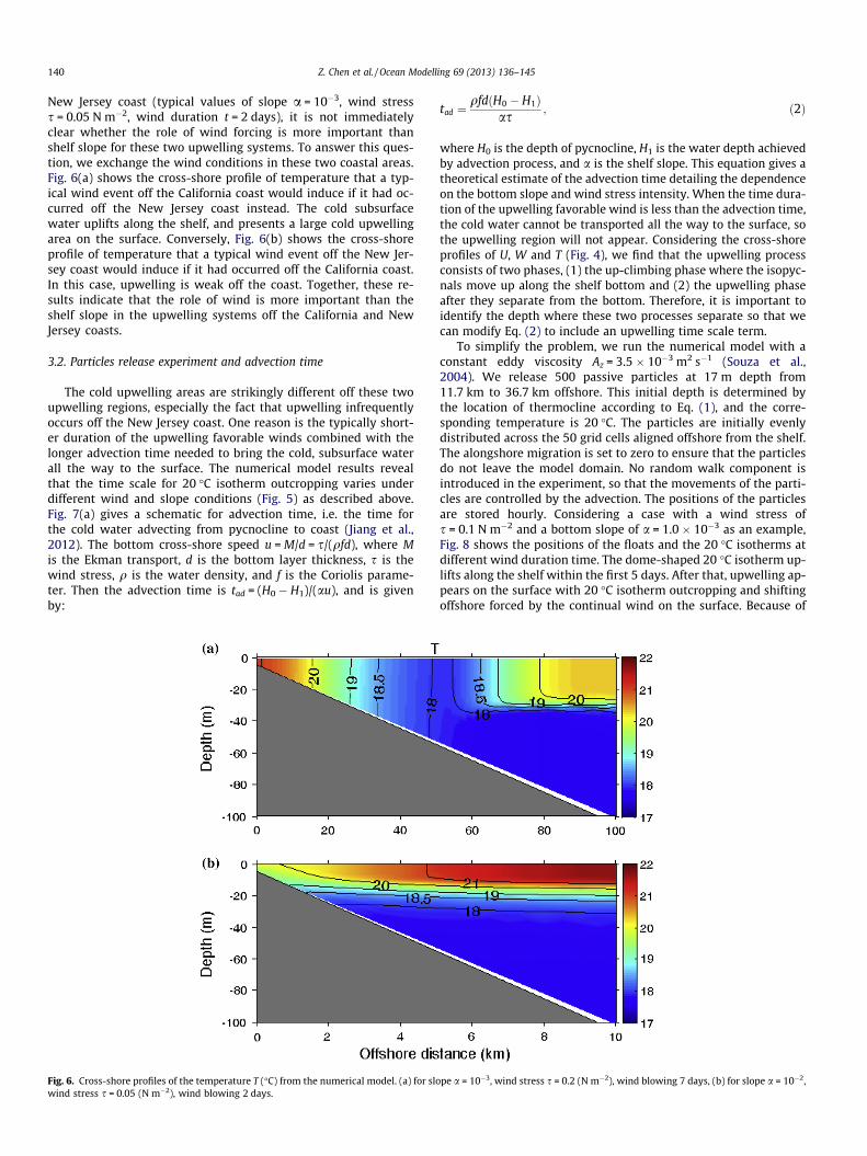
New Jersey coast (typical values of slope a = 10�3, wind stresss = 0.05 N m�2, wind duration t = 2 days), it is not immediatelyclear whether the role of wind forcing is more important thanshelf slope for these two upwelling systems. To answer this ques-tion, we exchange the wind conditions in these two coastal areas.Fig. 6(a) shows the cross-shore profile of temperature that a typ-ical wind event off the California coast would induce if it had oc-curred off the New Jersey coast instead. The cold subsurfacewater uplifts along the shelf, and presents a large cold upwellingarea on the surface. Conversely, Fig. 6(b) shows the cross-shoreprofile of temperature that a typical wind event off the New Jer-sey coast would induce if it had occurred off the California coast.In this case, upwelling is weak off the coast. Together, these re-sults indicate that the role of wind is more important than theshelf slope in the upwelling systems off the California and NewJersey coasts.

3.2. Particles release experiment and advection time

The cold upwelling areas are strikingly different off these twoupwelling regions, especially the fact that upwelling infrequentlyoccurs off the New Jersey coast. One reason is the typically short-er duration of the upwelling favorable winds combined with thelonger advection time needed to bring the cold, subsurface waterall the way to the surface. The numerical model results revealthat the time scale for 20 �C isotherm outcropping varies underdifferent wind and slope conditions (Fig. 5) as described above.Fig. 7(a) gives a schematic for advection time, i.e. the time forthe cold water advecting from pycnocline to coast (Jiang et al.,2012). The bottom cross-shore speed u = M/d = s/(qfd), where Mis the Ekman transport, d is the bottom layer thickness, s is thewind stress, q is the water density, and f is the Coriolis parame-ter. Then the advection time is tad = (H0 � H1)/(au), and is givenby:

Fig. 6. Cross-shore profiles of the temperature T (�C) from the numerical model. (a) for slowind stress s = 0.05 (N m�2), wind blowing 2 days.

tad ¼qfdðH0 � H1Þ

as; ð2Þ

where H0 is the depth of pycnocline, H1 is the water depth achievedby advection process, and a is the shelf slope. This equation gives atheoretical estimate of the advection time detailing the dependenceon the bottom slope and wind stress intensity. When the time dura-tion of the upwelling favorable wind is less than the advection time,the cold water cannot be transported all the way to the surface, sothe upwelling region will not appear. Considering the cross-shoreprofiles of U, W and T (Fig. 4), we find that the upwelling processconsists of two phases, (1) the up-climbing phase where the isopyc-nals move up along the shelf bottom and (2) the upwelling phaseafter they separate from the bottom. Therefore, it is important toidentify the depth where these two processes separate so that wecan modify Eq. (2) to include an upwelling time scale term.

To simplify the problem, we run the numerical model with aconstant eddy viscosity Az = 3.5 � 10�3 m2 s�1 (Souza et al.,2004). We release 500 passive particles at 17 m depth from11.7 km to 36.7 km offshore. This initial depth is determined bythe location of thermocline according to Eq. (1), and the corre-sponding temperature is 20 �C. The particles are initially evenlydistributed across the 50 grid cells aligned offshore from the shelf.The alongshore migration is set to zero to ensure that the particlesdo not leave the model domain. No random walk component isintroduced in the experiment, so that the movements of the parti-cles are controlled by the advection. The positions of the particlesare stored hourly. Considering a case with a wind stress ofs = 0.1 N m�2 and a bottom slope of a = 1.0 � 10�3 as an example,Fig. 8 shows the positions of the floats and the 20 �C isotherms atdifferent wind duration time. The dome-shaped 20 �C isotherm up-lifts along the shelf within the first 5 days. After that, upwelling ap-pears on the surface with 20 �C isotherm outcropping and shiftingoffshore forced by the continual wind on the surface. Because of

pe a = 10�3, wind stress s = 0.2 (N m�2), wind blowing 7 days, (b) for slope a = 10�2,

Fig. 7. Schematics for the advection time tad, (a) proposal from Jiang et al. (2012); (b) Eq. (3) of this study.

Fig. 8. Temporal evolution of the floats (dashed line) released at 17 m and the 20 �Cisotherms (solid line) (unit: day). Thick line is the trajectory of the fastest particle.

Z. Chen et al. / Ocean Modelling 69 (2013) 136–145 141

the diffusion processes, the water particles originated from thethermocline are warmer (colder) than 20 �C along the upwellingchannel, resulting in the 20 �C isotherm behind (before) to thepositions of the floats at the front (two wings). The friction andhorizontal diffusion make the water temperature near bottomshelf closer to the upwelling cell. Although the diffusion processesaffect the water temperature pattern to some extent, the advectionprocess dominates the coastal upwelling circulation in the trans-port of cold water. Therefore, the time scale of the floats advectingto the surface is approximate to that of thermocline outcropping.

Fig. 9 shows the Lagrangian cross-shore and vertical velocityfields derived from the trajectory of particles within the model

Fig. 9. (a) Cross-shore velocity U (m s�1) and (b) vertical velocity W (m s�1) calculated fline is the trajectory of the fastest particle. Dashed line describes the switch-over depth

after 15 days. First, the particles climb up the shelf, and then aretransported offshore after they cross the region between the sur-face mixed layer and bottom Ekman layer. The particles near bot-tom shelf cover the surface after model runs for 15 days, whileparticles near geostrophic interior are advected in a short distance.The particles are still initially, and accelerate continuously alongthe shelf. After reaching a maximum value at �12 m, they slowdown because of the decrease of W up to the surface. The fastestparticle, marked in thick line, tracks along the maximum verticalvelocity for each z level in the ‘‘up-climbing’’ process, and only be-gins to deviate from it after crossing the location of the directiontransition of cross-shore velocity. The fastest particle climbs upthe shelf, advects onshore within the bottom friction layer, andthen upwells and is transported offshore when it reaches the sur-face Ekman layer. Because the surface Ekman layer thickness islimited by the shallow water on the inner-shelf, the model resultsindicate that the switch-over depth for these two processes is lo-cated at approximately 0.9DE (DE ¼

ffiffiffiffiffiffiffiffiffiffiffiffi2Az=f

pis the Ekman depth)

and is independent of the shelf slope and the wind strength andduration under the assumption of constant eddy viscosity. There-fore, without the consideration of the effects of mixing and diffu-sion, Eq. (2) can be adjusted to be:

tad ¼qfdðH0 � H1Þ

asþ H1 � H2

W; ð3Þ

where H1 is the switch-over depth between the up-climbing andupwelling processes, �0.9DE, H2 is the depth to which the fastestparticle reaches after these two processes (also see Fig. 7(b) forthe schematic), d ¼ p

ffiffiffiffiffiffiffiffiffiffiffiffi2Az=f

pis the bottom friction layer thickness,

W = s/(qfL) is the averaged vertical velocity over the upwelling re-gion, and L is the length scale of WSED, which we take

L ¼ 0:75pffiffiffiffiffiffiffiffi2Azp

=ffiffiffif

pa

� �in this study (Estrade et al., 2008). The first

rom the trajectory of the released particles. Thin line marks zero velocity, and thickof the up-climbing and upwelling processes.

142 Z. Chen et al. / Ocean Modelling 69 (2013) 136–145

term is the climbing time scale, and later term relates to upwellingtime scale. Both of these time scales are inversely proportional toshelf slope and intensity of wind stress. Note that we only considerthe advection effect, the particle moving to the depth H2 is regardedas having arrived at the sea surface. For simplicity, we define H0 asthe depth of thermocline rather than pycnocline, and take advan-tage of the fact that it is more convenient to observe the cold waterappearing at the surface from the satellite images.

The numerical model with a constant eddy viscosity is used tovalidate the shelf slope and wind stress effects on the advectiontime as theorized in Eq. (3). Since the eddy viscosity is a constant,H1 is invariant �0.9DE in all cases, and we find H2 = 0.35DE, �3 mbased on the particle release experiments. The climbing andupwelling times are determined by time for the 20 �C isothermuplifting from H0 (thermocline depth) to H1 (transition depth),and H1 to H2, respectively. The dependence of the climbing andupwelling times on different slopes and wind stress intensitiesare shown in Fig. 10. Wind stress is fixed to 0.05 N m�2 whenchecking the slope effect (Fig. 10(a)), and slope is fixed to 10�3

when checking the wind effect (Fig. 10(b)). The results from thenumerical simulations (closed symbols) agree reasonable well withthe theoretical values calculated from Eq. (3) (open symbols), andshow approximately an inverse proportionality to both shelf slopeand wind stress intensity. The relationships in numerical model re-sults are not as strictly linear as that derived from Eq. (3), whichmay be due to the model spin-up and diffusion processes, e.g.the weaker the wind stress, more time the spin-up process needs.Gradual shelf slope and weaker wind stress both lead to largerclimbing and upwelling advection times, meaning that a longerduration of upwelling favorable winds is needed to advect the coldwater all the way to the surface. Comparing the climbing time

Fig. 10. Advection time in (a) different slopes and (b) different wind stressconditions: climbing advection time (circles), and upwelling advection time(triangles), where closed signs for numerical model, and open signs for theoreticalvalues. The eddy viscosity is a constant in all the cases (Az = 3.5 � 10�3 m2 s�1).

(circles) to the upwelling time (triangles) shows that the majorityof the total advection time is spent on climbing the slope, and thesetimes are related to the vertical velocity and the thickness of sur-face Ekman layer on the inner-shelf. Note that Eq. (3) is only anestimate of the advection time; numerical models and observa-tions are needed to further obtain an exact advection time in spe-cific upwelling regions.

4. Discussion

Using an analytic solution, Estrade et al. (2008) pointed out that

the scale of the WSED was L ¼ 0:75pffiffiffiffiffiffiffiffi2Azp

=ffiffiffif

pa

� �. To examine the

relationship between L and wind strength, we average the expo-nential eddy viscosity profile (Long, 1981; Lentz, 1995) in a scaleof turbulent boundary layer d to determine a typical value:

Az ¼R d

0 ku�z0 exp �z0l

� �dz0

d; ð4Þ

where d = ku⁄/f, k = 0.4 is the Von Karman constant, u� ¼ffiffiffiffiffiffiffiffiffis=q

pis

the shear velocity, z0 is the distance from the boundary, andl = 0.27d is the exponential decay scale. From Eq. (4), it can be foundthe eddy viscosity Az � 0.01s/(qf), meaning Az / s. Then, the WSEDis proportional to

ffiffiffisp

and 1/a. This implies that greater windstrength and gentle shelf slope correspond to larger WSED. Wehypothesize that the upwelling process is two-dimensional, the vol-ume of the upwelled water must be exactly equal to the offshoretransport. Consequently, the averaged vertical velocity within the

WSED is given by W ¼ M=L ¼ sa= 0:75pqffiffiffiffiffiffiffiffiffi2fAz

p� �. In this case, W

is proportional to a andffiffiffisp

. This implies that vertical velocity ispositively correlated to shelf slope and wind strength. These arethe reasons for the vertical velocity structures response to windstrength and shelf slope in Fig. 4. The theoretical expressions ofthe WSED and vertical velocity are based on a constant eddy viscos-ity controlled by the wind stress. The eddy viscosity in the numer-ical model, calculated by the MY-2.5 turbulent closure scheme, issmall in the geostrophic interior. The location and WSED are sensi-tive to the eddy viscosity profile, and the weaker eddy viscosityinterior produces narrower WSED in shallower water comparingto the eddy viscosity profiles with larger values (Lentz, 1995).Therefore, the theoretical values given by a constant eddy viscosityaveraged in the whole water column will overestimate the WSED,and underestimate the vertical velocity.

The model experiments show that stronger wind stress, steeperbottom slope, and longer wind duration result in upwelling eventswith a larger vertical velocity and more extensive cold water area.Therefore, the vertical velocity is expected to be larger in the Cal-ifornia upwelling system than in that off the New Jersey coast.Off the California coast, the stronger wind stress acts to increasethe WSED, whereas the steeper bottom slope acts to decrease it.The large area of cold water off the California coast observed in sa-tellite images can be attributed to stronger wind stress, longerwind duration and steeper bottom slope, which lead to shorteradvection time. Stronger wind stress drives a larger offshore trans-port, which leads to an upwelling front that is further offshore(Fig. 4(i) vs. (f)). With respect to the effect of shelf slope, it takesa longer time for the subsurface water to advect to the surface overa gradual slope because of the longer advection distance and smal-ler vertical velocity. After the cold water outcrops, the propagationspeed of the upwelling front, which is controlled by the magnitudeof the transport in the surface Ekman layer, is independent of theshelf slope.

The variation and trend of upwelling north of off San Franciscoon the U.S. west coast are positively related to the equatorwardwind (Seo et al., 2012). The variations in SST caused by upwelling

Z. Chen et al. / Ocean Modelling 69 (2013) 136–145 143

off the central California are correlated with both changes in windand the climate indices (García-Reyes and Largier, 2010). Off theNew Jersey coast, the currents are significantly coherent with thewind with an offshore (onshore) flow in the upper (lower) layerwhen the wind is upwelling favorable (Wong, 1999). During anupwelling favorable wind pulse, cold water is brought to the sur-face through the bottom boundary layer in the manner of Ekmandynamics on the New Jersey shelf (Yankovsky, 2003). Therefore,the winds are the dominant effect on coastal upwelling processesin this two regions, although mesoscale eddies have influenceson shaping the eastern boundary upwelling systems dynamicalstructure (Capet et al., 2008) and filament structure are dependenton local processes in the California Current System (Penven et al.,2006), the roles of which are beyond the extent of this study.

By late spring, coastal upwelling strengthens and reaches itsmaximum in June, weakens by late summer and ends in October.April–August is regarded as the spring-summer upwelling season(Huyer and Kosro, 1987). Off the New Jersey coast, the Bermuda/Azores high builds into the southeast by April, and southerly(upwelling favorable) winds are prevalent from May to September,while westerly and northwesterly (upwelling unfavorable) windsare prevalent in the winter (Klink, 1999). In upwelling season,the stratification is weak with deep pycnocline off the Californiacoast, while it reverses off the New Jersey coast, but the Burgernumber is �0.7 for both regions, indicating the similar effect ofstratification in the subtidal frequency dynamics (Jiang et al.,2012). In periods of strong wind driven upwelling events, thealongshore wind stress is changeable in a range of �0.4 to0.1 N m�2 (positive northward) with typical wind duration periodof 7–10 days off the California coast (Huyer and Kosro, 1987).The wind stress has high-frequency variability in a range of�0.08 to 0.08 N m�2 with wind events period of 1–3 days off theNew Jersey coast in May–August, 1996 (Yankovsky and Garvine,1998). Jiang et al. (2012) used an idealized numerical model toestimate the advection time for both coasts and found it to be0.5 days for the Oregon coast and 3 days for the New Jersey coast.It takes two days of upwelling-favorable wind to cause the pycno-cline to outcrop off the New Jersey coast (Yankovsky, 2003), whilethe surface temperature and salinity respond to the variations ofthe alongshore wind within one day during upwelling events offthe California coast (Huyer, 1984). It is important to note thatthe wind duration time often exceeds the advection time overthe California shelf, but not over the New Jersey shelf in upwellingseason. Thus the condition is more upwelling-favorable off the Cal-ifornia coast than off the New Jersey coast. This tendency is quan-tified by the proxy of upwelling age. When it is less than 1, theupwelling front cannot form at the surface. If it exceeds 1, anupwelling area appears. The larger C is, the stronger upwellingtendency will be.

The results in Figs. 1 and 6 can be explained by upwelling agetheory: the ratio of the wind duration in these two upwelling sys-tems is 7:2, and that of wind stress intensity is 4:1. Since tad / 1/s,the ratio of the wind contribution to the upwelling age in these twoupwelling systems is 14:1. While, the ratio of slope effect contrib-uted to the upwelling age in these two upwelling systems is only10:1, which is smaller than the wind effect. Consequently, thenet ratio of upwelling age for the California and New Jersey upwell-ing systems is roughly 140:1, which explains the reason for theenormous difference between the extents of the cold upwellingareas off each coast observed in satellite SST images. Of course,for the New Jersey coast, the upwelling region will appear if theduration of upwelling favorable wind is long enough, rather thanthe wind direction shifting back and forth, although it is restrictedby the wide and shallow continental shelf. Note that the linearrelationship between the advection time and wind duration, windstress, shelf slope is based on the assumption of the homogenous

ocean in the idealized condition. The complicated coastline,bathymetry, eddies, currents, etc. will make the upwelling pro-cesses more intricate response to the wind and shelf, and this lin-ear relationship shall be elaborated and modified.

The advection time in Eq. (3) is derived from one-dimensionalEkman theory, assuming a constant eddy viscosity. However, inthe real ocean, eddy viscosity varies from surface to bottom withinthe range of 10�3 to 10�2 m2 s�1 (Souza et al., 2004), and is influ-enced by wind stress, bottom stress, stratification, etc. The varia-tions of magnitude and direction of the wind stress result in thechange of the switch-over depth, H1, and the vertical velocity.The interaction of the surface and bottom boundary layers andinteractive response of wind-driven cross-shelf circulation to dif-ferent topographic forcing are complex (Gan et al., 2009). Further,the bottom layer thickness, d, and bathymetry vary in differentcoastal areas, such as off the northwestern Africa, northern Califor-nia, Oregon, and Peru (Smith, 1981). Therefore, it becomes morecomplicated to estimate the advection time in different upwellingregions. Meanwhile, the deeper pycnocline in winter will result ina larger climbing advection time. All of these factors influence theadvection time in a real upwelling system. Nevertheless, Eq. (3)gives an estimate for the advection time consisting of climbingand upwelling processes, and shows the relative effects of shelfslope and wind stress. It is more difficult to advect the cold waterto the surface (i.e. the advection time is larger) with weaker windstress over gradually sloping shelf like that off the New Jerseycoast. On the inner-shelf, because of limited water depth, the bot-tom and surface Ekman layers interact with each other. Accordingto the idealized Lagrangian particle experiments, the cold subsur-face water advects onshore to the inner-shelf until it reaches adepth of �0.9DE, where it is upwelled and then transported off-shore. First, the kinetic energy of the wind is used to transport coldwater from pycnocline to the surface, and there is no obvious tem-perature drop off the coastal region. After that, the remaining dura-tion of upwelling favorable wind drives the upwelling frontoffshore and presents a cold upwelling area.

5. Conclusions

In this study, we compare the upwelling systems off the Califor-nia and New Jersey coasts with regards to the contribution of windstress intensity, wind duration and shelf slope to the differentupwelling intensities in these two areas. An idealized numericalmodel simulation is used to study these effects on wind-drivencoastal upwelling. The model results show that stronger windstress leads to a deeper Ekman layer depth and a larger offshorevelocity, which leads to the formation of a larger cold upwellingarea, whereas, the bottom slope effect on them is negligible. Steepslope and weak wind lead to narrow WSED, while steep slope andgreat wind strength lead to large vertical velocity. For the case ofstrong wind stress over a gradual shelf slope, the maximum verti-cal velocity, and consequently the position where the isothermfirst outcrops, appears farther from the coast.

We extend the definition of advection time, which is the mainconcept within upwelling age theory, to differentiate betweenclimbing and upwelling time scales. Climbing time is the time scalefor cold water to climb up the slope from the pycnocline to thedepth where it leaves the bottom, and upwelling time is the timescale for the cold water to rise from the bottom to the surface. Boththese time scales, expressed by Eq. (3), are inversely proportionalto shelf slope and wind stress. Through Lagrangian particle releaseexperiments in the idealized numerical model with constant eddyviscosity, we find that the switch-over depth for these two pro-cesses is located at �0.9DE. When the duration of wind forcing isless than the advection time scale, upwelling front will not appear

144 Z. Chen et al. / Ocean Modelling 69 (2013) 136–145

off the coast. If the duration of upwelling-favorable wind exceedsthe advection time scale, isopycnals outcrop and an upwellingfront is formed. The larger ratio of wind duration time to theadvection time denotes stronger upwelling tendency. For steepershelves, less advection time is needed because a shorter horizontaldistance is required to transport cold water to the surface. Thestronger wind stress increases the cross-shore velocity and Ekmantransport, leading to a reduction of the advection time. Therefore,the expression of the ‘‘upwelling age’’, C, is:

C ¼ twind

tad¼ twind

qfdðH0�H1Þas þ H1�H2

W

; ð5Þ

where twind is the upwelling favorable wind duration.The California coastal region is considerably more favorable to

the development of upwelling because of stronger wind stress,longer duration of upwelling favorable winds and a steeper shelfcompared to conditions off the New Jersey coast. As an applica-tion of the model results and upwelling age theory, theexchanged wind forcing experiments show that a large coldupwelling area would appear off the New Jersey coast underCalifornia wind conditions, while much less cold water wouldupwell to the surface in the converse case of New Jersey windconditions imposed off the California coast. These results indicatethat the role of wind is the dominant factor in determining theupwelling intensity in these two areas. Further, the applicationof the upwelling age concept adequately explains the differencesin upwelling features between the east and west coasts of the U.S.The less advection time results in upwelling phenomenon, as wellas the related biological and chemical processes, rapider responseto alongshore wind off the California coast. Although the roles ofwind and topography on upwelling are studied to some extentabout upwelling age here, the effects of eddy and filamenttransport, variable eddy viscosity and model spin-up processeson the advection time, and therefore upwelling age need furtherelaborate study.

Acknowledgments

This study was partially supported by NASA Physical Oceanog-raphy and EPSCoR Programs and by NOAA Sea Grant in U.S.; by 973Program (2009CB421200, 2013CB955700) from the National BasicResearch Program of China, and by the Natural Science Foundationof China (Grant No. 41076001), and the Fundamental ResearchFunds for the Central Universities (Grant No. 2010121029) in Chi-na. We would like to thank R.W. Garvine and L.C. Breaker for theinitial idea on the comparison of upwelling off the eastern andwestern U.S. coasts in an early collaborative NSF proposal. We alsothank the two anonymous reviewers for helpful comments on themanuscript.

References

Allen, J.A., Newberger, P.A., Federick, J., 1994. Upwelling circulation on the Oregoncontinental shelf, part 1: response to idealized forcing. Journal of PhysicalOceanography 25, 1843–1866.

Breaker, L.C., Mooers, C.N.K., 1986. Oceanic variability off the central Californiacoast. Progress in Oceanography 17, 61–135.

Capet, X., Colas, F., McWilliams, J.C., Penven, P., Marchesiello, P., 2008. Eddies ineastern boundary subtropical upwelling systems. In: Hecht, M.W., Hasumi, H.(Eds.), Ocean Modeling in an Eddying Regime, Geophysical Monograph Series,vol. 177. AGU, Washington, DC, pp. 131–147. http://dx.doi.org/10.1029/177GM10.

Choboter, P.F., Duke, D., Horton, J.P., Sinz, A.P., 2011. Exact solutions of wind-drivencoastal upwelling and downwelling over sloping topography. Journal ofPhysical Oceanography 41, 1277–1296.

Clarke, A.J., Brink, K.H., 1985. The response of stratified, frictional flow of shelf andslope waters to fluctuating large-scale, low-frequency wind forcing. Journal ofPhysical Oceanography 15, 439–453.

Estrade, P., Marchesiello, P., Verdière, A.C.D., Roy, C., 2008. Cross-shelf structure ofcoastal upwelling: a two-dimensional extension of Ekman’s theory and amechanism for inner shelf upwelling shut down. Journal of Marine Research 66,589–616.

Gan, J., Cheung, A., Guo, X., Li, L., 2009. Intensified upwelling over a widened shelf inthe northeastern South China Sea. Journal of Geophysical Research 114, C09019.http://dx.doi.org/10.1029/2007JC004660.

García-Reyes, M., Largier, J., 2010. Observations of increased wind-driven coastalupwelling off central California. Journal of Geophysical Research 115, C04011.http://dx.doi.org/10.1029/2009JC005576.

Garvine, R.W., 2004. The vertical structure and subtidal dynamics of the inner shelfoff New Jersey. Journal of Marine Research 62, 337–371.

Gomez-Gesteira, M., Castro, M., Alvarez, I., Lorenzo, M.N., Gesteira, J.L.G., Crespoa,A.J.C., 2008. Spatio-temporal upwelling trends along the Canary UpwellingSystem (1967–2006). Trends and Directions in Climate Research 1146, 302–337. http://dx.doi.org/10.1196/annals.1446.004.

Huyer, A., 1984. Hydrographic observations along the CODE central line offnorthern California, 1981. Journal of Physical Oceanography 14, 1647–1658.

Huyer, A., Kosro, P.M., 1987. Mesoscale surveys over the shelf and slope in theupwelling region near Point Arena, California. Journal of Geophysical Research92, 1655–1681.

Jacox, M.G., Edwards, C.A., 2011. Effects of stratification and shelf slope on nutrientsupply in coastal upwelling regions. Journal of Geophysical Research 116,C03019.

Jiang, L., Yan, X.-H., Tseng, Y.-H., Breaker, L.C., 2011. A numerical study on the role ofwind forcing, bottom topography, and nonhydrostacy in coastal upwelling.Estuarine Coastal and Shelf Science 95 (1), 99–109. http://dx.doi.org/10.1016/j.ecss.2011.08.019.

Jiang, L., Yan, X.-H., Breaker, L.C., 2012. Upwelling age – an indicator of localtendency for coastal upwelling. Journal of Oceanography 68, 337–344. http://dx.doi.org/10.1007/s10872-011-0096-2.

Klink, K., 1999. Climatological mean and interannual variance of United Statessurface wind speed, direction and velocity. International Journal of Climatology19, 471–488.

Lentz, S.J., 1995. Sensitivity of the inner-shelf circulation to the form of the eddyviscosity profile. Journal of Physical Oceanography 25, 19–28.

Lentz, S.J., Trowbridge, J.H., 1991. The bottom boundary-layer over the NorthernCalifornia shelf. Journal of Physical Oceanography 21, 1186–1201.

Long, C.E., 1981. A simple model for time-dependent stably stratified turbulentboundary layers, Tech. Rep. Special Report, No. 95, pp. 170, University ofWashington, Seattle, Washington.

Melton, C., Washburn, L., Gotschalk, C., 2009. Wind relaxations and poleward flowevents in a coastal upwelling system on the central California coast. Journal ofGeophysical Research 114, C11016. http://dx.doi.org/10.1029/2009JC005397.

Narimousa, S., Maxworthy, T., 1986. Coastal upwelling on a sloping bottom: theformation of plumes, jets and pinched-off cyclones. Journal of Fluid Mechanics176, 169–190.

Penven, P., Debreu, L., Marchesiello, P., McWilliams, J.C., 2006. Evaluation andapplication of the ROMS 1-way embedding procedure to the central Californiaupwelling system. Ocean Modelling 12 (1–2), 157–187.

Pringle, J.M., Dever, E.P., 2009. Dynamics of wind-driven upwelling and relaxationbetween Monterey Bay and Point Arena: local-, regional-, and gyre-scalecontrols. Journal of Geophysical Research 114, C07003. http://dx.doi.org/10.1029/2008JC005016.

Rodrigues, R.R., Lorenzzetti, J.A., 2001. A numerical study of the effects of bottomtopography and coastline geometry on the Southeast Brazilian coastalupwelling. Continental Shelf Research 21, 371–394.

Seo, H., Brink, K.H., Dorman, C.E., Koracin, D., Edwards, C.A., 2012. Whatdetermines the spatial pattern in summer upwelling trends on the U.S. WestCoast? Journal of Geophysical Research 117, C08012. http://dx.doi.org/10.1029/2012JC008016.

Shchepetkin, A.F., McWilliams, J.C., 2005. The regional ocean modeling system: asplit-explicit, free-surface, topography-following coordinates ocean model.Ocean Modelling 9, 347–404.

Smith, R.L., 1968. Upwelling. In: Barnes, H. (Ed.), Oceanography and Marine Biology:An Annual Review, vol. 6. G. Allen & Unwin, London, pp. 11–46.

Smith, R.L., 1981. A comparison of the structure and variability of the flow field inthree coastal upwelling regions: Oregon, Northwest Africa, and Peru. In: CoastalUpwelling. American Geophysical Union, pp. 107–118.

Song, Y.T., Chao, Y., 2004. A theoretical study of topographic effects on coastalupwelling and cross-shore exchange. Ocean Modelling 6, 151–176. http://dx.doi.org/10.1016/S1463-5003(02)00064-1.

Song, Y.T., Haidvogel, D.B., 1993. Numerical simulations of the CCS under the jointeffects of coastal geometry and surface forcing. In: Spaulding, M.L. et al. (Eds.),Estuarine and Coastal Modeling. American Society of Civil Engineers, Reston,VA, pp. 216–234.

Song, Y.T., Haidvogel, D.B., 1994. A semi-implicit ocean circulation model using ageneralized topography following coordinate system. Journal of ComputationalPhysics 115, 228–244.

Song, Y.T., Haidvogel, D.B., Glenn, S., 2001. The effects of topographic variability onthe formation of upwelling centers off New Jersey: a theoretical model. Journalof Geophysical Research 106 (C5), 9223–9240.

Souza, A.J., Alvarez, L.G., Dickey, T.D., 2004. Tidally induced turbulence andsuspended sediment. Geophysical Research Letters 31, L20309. http://dx.doi.org/10.1029/2004GL021186.

Z. Chen et al. / Ocean Modelling 69 (2013) 136–145 145

Torres, R., Barton, E.D., Miller, P., Fanjul, E., 2003. Spatial patterns of wind and seasurface temperature in the Galician upwelling region. Journal of GeophysicalResearch 108, 3130–3143. http://dx.doi.org/10.1029/2002JC001361.

Wong, K.-C., 1999. The wind driven currents on the Middle Atlantic Bight innershelf. Continental Shelf Research 19, 757–773.

Yankovsky, A.E., 2003. The cold-water pathway during an upwelling event on theNew Jersey shelf. Journal of Physical Oceanography 33, 1954–1966.

Yankovsky, A.E., Garvine, R.W., 1998. Subinertial dynamics on the inner New Jerseyshelf during the upwelling season. Journal of Physical Oceanography 28, 2444–2458.