Rogue waves in large-scale fully-non-linear

High-Order-Spectral simulations

Guillaume Ducrozet, Felicien Bonnefoy & Pierre Ferrant

Laboratoire de Mecanique des Fluides - UMR CNRS 6598Ecole Centrale de Nantes

1, rue de la Noe, 44321 Nantes, Franceguillaume.ducrozet@ec-nantes.fr, felicien.bonnefoy@ec-nantes.fr,

pierre.ferrant@ec-nantes.fr

Abstract. This study is devoted to the simulation of 3D directionalwave fields with a fully-non-linear potential-flow model. This model isbased on the High-Order-Spectral (HOS) method in the consistent formof West et al. [14]. The accuracy and efficiency of this model give ac-cess to the fully-non-linear evolution of large domains during long pe-riod of time. Besides, the recent efficient parallelization of the code (seeDucrozet et al. [5]) allows us to run parametric studies. In this paper, theoccurrence of extreme waves is investigated within sea-states of differentcharacteristics.

Introduction

Extremely large waves are named freak or rogue waves when their height or crestamplitude exceed the significant wave height by a factor 2.2 or 1.4 respectively.Several ships and platforms have been confronted to such destructive waves inthe last decades (see eg. Didenkulova et al. [2] for a review of the accidents in-volving freak waves in 2005). However, accurate simulations of this 3D highlynon-linear process is still very challenging. Different mechanisms of formationof such events have been pointed out such as wave focusing, wave-current in-teractions, non-linear wave interactions, . . . (see Kharif and Pelinovsky [8] for areview). We focus in this paper on the long-time evolution of wave fields in deepwater without wind and current.

Many numerical models have been developed to study the freak waves oc-currence in the last fifty years. The pioneering work of Philipps who studied theenergy exchange resulting from wave interaction in the framework of a weakly-non-linear method, was followed by other numerical tools accounting for moreand more complexity. Zakharov [15] described the full time evolution equationsof the wave system which have been later solved using reduced expressions lim-ited to four-wave or five-wave interactions (see e.g. Stiassnie and Shemer [12]).The Non-Linear Schrodinger (NLS) equation (arising when the narrow-band as-sumption of the wave spectrum is added to the previous model) has also beenwidely used in this topic (see Trulsen and Dysthe [13] for the latest enhanced

version (Broad-Modified NLS - BMNLS) allowing broader bandwidth and fourthorder in wave steepness). However, as noticed in Kharif and Pelinovsky [8], roguewaves present large amplitudes, high steepness, and short duration. This breaksthe assumptions of weak non-linearity and narrow-banded spectrum. An inter-esting approach can then to use time-domain fully-non-linear potential models.Nonetheless, such numerical simulations are today still very challenging. Indeed,the Boundary Element Method (BEM), classically employed within the latterclass of methods, remains too slow to reproduce square kilometers of ocean long-time evolution.

Consequently, our study is based on an alternative approach, the High Or-der Spectral (HOS) method, proposed by West et al. [14] and Dommermuthand Yue [4]. This method allows the fully-non-linear simulation of gravity wavesevolution within 3D periodic domains. With respect to classical time-domainmodels such as the BEM, this spectral approach presents the two assets of itsfast convergence and its high computational efficiency (by means of Fast FourierTransforms FFTs), allowing to accurately simulate long-time 3-D sea state evo-lutions with fine meshes.

Firstly, we present the model used which is a parallelized version of theorder consistent HOS model of West et al. [14]. Specific attention has beenpaid to aliasing matter and numerical efficiency. A parallel version of the code(Ducrozet et al. [5]) is used, allowing fully-non-linear simulations of tens of squarekilometers during hundreds of periods without prohibitive CPU cost. The initialcondition is defined (through a given wave spectrum) and we let it evolve duringlong simulation time looking at natural appearance of rogue events. Typically,100 km2 of ocean are simulated over 500 peak periods (i.e. ' 1 h and 45 min.).The second part of the present paper is devoted to a parametric study of theinfluence of the mean steepness of the wavefield, i.e. Benjamin-Feir Index (BFI),on these extreme events occurrence. Comparisons between linear theory and ourfully-non-linear simulations are provided and will point out the main importanceof non-linearities.

1 Formulation

In this section we briefly present the HOS method used in the following large-scale simulations. The initialization of the wavefield is exposed as well as theapproach employed to detect the rogue waves. A recent paper, Ducrozet et al.[6], shows the ability of this model to simulate freak waves appearance and a firstparametric study on the influence of directionality on freak waves occurrence wasproposed. We refer to this paper for more details about the HOS method.

1.1 Hypothesis and equations

We consider an open periodic fluid domain D representing a rectangular part ofthe ocean of infinite depth h→ ∞. We choose a cartesian coordinate system with

the origin O located at one corner of the domain. Horizontal axes are alignedwith the sides of the domain and (Lx, Ly) represent the dimensions in x− andy−directions respectively. x stands for the (x, y) coordinates. The vertical axisz is orientated upwards and the level z = 0 corresponds to the mean water level(see Fig. 1).

PSfrag replacements

LxLy

xy

z

O

−h

Fig. 1. Sketch of the domain with coordinate system

The fluid is assumed incompressible and inviscid. The wave-induced mo-tion of the fluid is described by an irrotational velocity and we assume that nowave-breaking occurs. Under these assumptions, the flow velocity derives froma velocity potential φ(x, z, t) satisfying the Laplace’s equation inside the fluiddomain D.

∆φ = 0 inside D (1)

Following Zakharov (1968) , the fully-non-linear free surface boundary con-ditions can be written in terms of surface quantities, namely the single-valuedfree surface elevation η(x, t) and the surface potential φs(x, t) = φ(x, η, t).

∂φs

∂t= −gη − 1

2|∇φs|2 +

1

2

(1 + |∇η|2

)(∂φ∂z

)2

(2)

∂η

∂t=(1 + |∇η|2

) ∂φ∂z

− ∇φs · ∇η (3)

both expressed on z = η(x, t) with W = ∂φ/∂z(x, η, t). The unknowns η and φs

are then time-marched with a 4th order Runge-Kutta scheme with an adaptativestep-size control. The only remaining unknown in Eqs (2) and (3) is the verticalvelocity W which is evaluated by the order-consistent HOS scheme of West etal. [14].

1.2 High-Order-Spectral method

The HOS method consists in expanding the velocity potential located at theexact free surface position in a combined power of η and Taylor series about themean water level z = 0 prior to compute its vertical derivative. The products

involving ∇η and W in Eqs. (2) and (3) are evaluated thanks to the orderconsistent formulation of West et al. [14].

This method is based on an iterative process (up to the so-called HOS orderM) to evaluate the vertical velocity W . This quantity W is the only one thatis approximated in the free surface boundary conditions whose non-linearitiesare otherwise fully accounted for. The non-linear terms are conserved and theboundary conditions expressed on the exact free surface position η(x, t)).

The HOS formulation provides a very efficient FFT-based solution schemewith numerical cost growing as Nlog2N , N being the number of modes. Anacceleration procedure, based on an analytical integration of the linear part ofthe equations, has also been implemented. Non-linear products are evaluatedin the spatial domain with special care paid to dealiasing while derivatives areevaluated in the Fourier domain.

Periodic boundary conditions are applied in both direction x and y to theunknowns η, φs and the potential φ. These conditions added to the infinite depthcondition as well as the Laplace’s equation (1) are used to define the spectralbasis functions on which φ is expanded. The unknowns η and φs are accordinglyexpanded on the Fourier basis.

Finally, notice that a parallel version of the code has been recently developedwhich allows the use of memory-distributed supercomputers. More details aboutthe parallelization and particularly about its great efficiency can be found inDucrozet et al. [5]. Simulations presented later on have been performed withthis parallel version.

1.3 Initial condition

The initial wavefield is defined by a directional wave spectrum S(ω, θ) = ψ(ω)×G(θ) where the frequency spectrum is chosen as a modified JONSWAP one

(space and time are normalized respectively with scales L = 1/kp and T =√L/g

where kp is the peak wavenumber).

ψ(ω) = αg2ω−5 exp

(−5

4

[ω

ωp

]−4)γ

exp

[−

(ω−ωp)2

2σ2ω2p

]

(4)

with ωp the angular frequency at the peak of the spectrum and

α = 3.279E, γ = 3.3, σ =

{0.07 (ω < 1)0.09 (ω ≥ 1)

(5)

The dimensionless energy E of the wavefield is related to the significant waveheight Hs by Hs ' 4

√E. The directionality function is defined by:

G(θ) =

1β cos2

(πθ

2β

), |θ| ≤ β

0 , |θ| > β(6)

with β a measure of the directional spreading. In the following, we study onlylong crested wave fields, with β = 0.26 which corresponds to a directional spread

of 14.9◦ or almost equivalent to directional function cos2s(θ), with s = 45.

Then, the initial free surface elevation η and free surface velocity potentialφs are computed from this directional spectrum definition by a superposition oflinear components with random phases. It is to notice that a linear initializationof a fully-non-linear simulation can lead to numerical instabilities. Thus, the re-laxation scheme of Dommermuth [3] is used at the beginning of the computationfor the transition from the linear wavefield to the realistic fully-non-linear one.

1.4 Detection of rogue waves

The rogue waves are generally defined as waves whose height H exceeds thesignificant wave height Hs by a given factor (typically 2.2) or waves whose crestheight Ac exceeds Hs in a given proportion. To apply such a criterion, we haveto define and measure the waves height or crest height from the free surfaceelevation η. Firstly, we define the wave height in our 3D simulations as theheight of a wave in the mean direction of propagation. Then, we perform a zeroup-and-down crossing analysis on each mesh line aligned with the x-axis whichis the mean direction of propagation of our wavefield. Afterwards, a transversezero up-and-down crossing analysis is performed, along the y-axis this time. Thisdouble zero-crossing analysis allows us to extract each 3−D wave and to describeit in both horizontal directions with its wavelength λx, crest length λy and alsothe crest and trough heights. The significant wave height is calculated fromthe standard deviation σ of the free surface elevation η (Hs = 4σ). Among thedetected waves, we are able to locate the freak events, determine their dimensionsand characteristics by applying one of the above criteria.

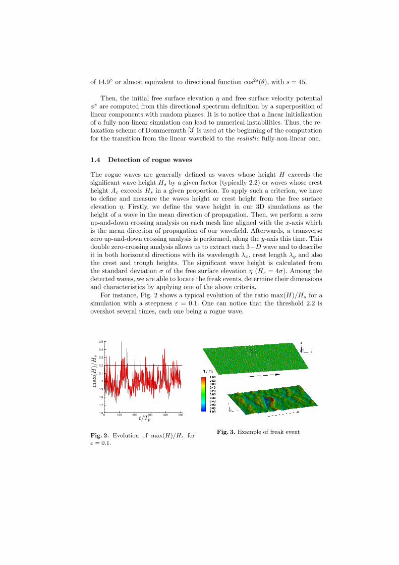
For instance, Fig. 2 shows a typical evolution of the ratio max(H)/Hs for asimulation with a steepness ε = 0.1. One can notice that the threshold 2.2 isovershot several times, each one being a rogue wave.

0 100 200 300 400 5001.6

1.7

1.8

1.9

2

2.1

2.2

2.3

2.4

2.5

PSfrag replacements

max(H

)/H

s

t/Tp

Fig. 2. Evolution of max(H)/Hs forε = 0.1.

Fig. 3. Example of freak event

Once the freak wave is detected inside the domain, it is possible to analyze itsshape, crest and trough height, i.e. all its characteristics. An example of detectedextreme event is presented on Fig. 3. Top part of the figure represents the wholesimulated domain (the white square encloses the detected extreme event) whilethe bottom part is a zoom on this event which exhibits a ratio H/Hs = 2.48.

The arrows indicate the mean direction of propagation of the wavefield whilethe colors give the free surface elevation. The freak wave (which height is 12.7m for Hs = 5.12 m if we choose Tp = 12.5 s) is a huge wave crest followed by adeep trough. One can see the exceptional feature of this wave compared to thesurrounding waves.

2 Influence of the mean steepness

Using the numerical model described in the previous sections, we study the in-fluence of the mean steepness of the wave field on the formation of freak wavesduring the evolution of a given wave spectrum. Thus, one lets evolve this giveninitial 3D sea-state which is analyzed to extract different waves and study theirproperties. Firstly, the linear theory for the freak waves occurrence in 3D wave-fields is briefly exposed. Then, the set of simulations used to study the influenceof mean steepness is presented. We notice the importance of spectral broadeningduring simulations, leading to an enhanced linear theory, and finally, we presentthe results obtained, pointing out the influence of non-linearities in the roguewaves phenomenon.

The following numerical conditions are common to all the performed simulations:

– Domain area: Lx × Ly = 42λp × 42λp, with λp the peak wavelength,– Number of modes: Nx × Ny = 1024 × 512,– HOS order M = 5, full dealiasing,– Duration of simulations: 500Tp (with Tp being the peak period).

The energy density E will be defined later.

2.1 Linear model

Baxevani and Rychlik [1] studied the probability of occurrence of extreme eventsin a Gaussian framework. Particularly, they provided an upper bound for theprobability of wave crests height (Ac) exceeding a given level u in a regionof space during a period of time. This upper bound is given by the followingequation:

P [Ac > u] ≤ P [X(0) > u] +

(Lx

λx+

Ly

λy+

T

Tz

)e−8u2/H2

s

+√

2π

(Nt + Ny

√1 − α2

xt + Nx

√1 − α2

yt

)4u

Hse−8u2/H2

s

+2πN√

1 − α2xt − α2

yt

(4u

Hs

)2

e−8u2/H2s (7)

where Tz is the average wave period and for our purpose, N = LxLyT/(λxλyTz),Nx = LyT/(λyTz), Ny = LxT/(λxTz) and Nt = LxLy/(λxλy). The parametersαxt and αyt accounts for drift velocity; we have αxt = 0.89 as we use a JONSWAPspectrum and αyt = 0 due to symmetry of the directional spreading. We invite torefer to Baxevani and Rychlik [1] for details concerning this equation. We noticehere that they also pointed out the influence of the spreading of waves on theseoccurrences: considering waves moving along one direction (i.e. 2D calculations)can lead to substantial underestimations.

Consequently, to be consistent with this formulation, the definition of freakwaves has to be adapted to define the corresponding exceedance on the ratiomax(Ac)/Hs. Taking as basis the observation of Guedes Soares et al. [10], onechooses to use the vertical asymmetry parameter: max(Ac) ≥ 1.4Hs. Thus, oneevaluates the return period of such a wave (i.e. the time required to record sucha wave within our simulation domain) from equation (7). We obtain that in alinear framework, in a domain like the one simulated here (42λp × 42λp), thereturn period of rogue waves is 360Tp or equivalently ' 60.000 waves. Thatis to say, the linear theory predicts that a freak wave can eventually appearduring our 500 Tp simulations. For the comparisons made with the linear theoryof Baxevani and Rychlik, the analysis of this ratio max(Ac)/Hs is chosen as adetection criterium for the extreme events.

2.2 Description of the non-linear simulations

We performed simulations with varying steepness as reported in Tab. 1. It is tonotice that a small filtering is applied to the most extreme case (E = 5 . 10−3)to prevent from wave breaking during simulations: this explains the slight differ-encies one could observe at beginning of simulations (Fig. 5). Table 1 contains

the mean steepness of the wave field ε = kpa, with a =(2 < η2 >

)1/2(i.e.

ε = kpHs/2√

2) and the Benjamin-Feir Index (BFI) defined by

BFI =2ε

σω

where σω is the bandwidth of the spectrum. This index plays a key role inthe wave-wave interactions (Alber, 1978) and characterizes the stability of wavetrains.

2.3 Spectral broadening

During the evolution of the wavefield, we observe that the non-linear wave inter-actions induce changes in the wave spectrum. As it has been previously studiedwith several numerical methods (for instance with advanced NLS models inSocquet-Juglard et al. [11]) the spectrum broadens in the transverse directionand the spectrum peak is downshifted. Figure 4 shows a typical evolution of thespectrum for a steepness ε = 0.1. The left part of the figure presents the initial

E ε BFI

5 . 10−5 0.01 0.10

5 . 10−4 0.032 0.33

1 . 10−3 0.045 0.46

2 . 10−3 0.063 0.65

3 . 10−3 0.077 0.80

5 . 10−3 0.10 1.03Table 1. Simulations parameters

0 0.5 1 1.5 2-1

-0.5

0

0.5

1

0 0.5 1 1.5 2-1

-0.5

0

0.5

1

PSfrag replacements

kx/kpkx/kp

ky/k

p

ky/k

p

t = 0Tp t = 260Tp

Fig. 4. Spectral broadening for a long crested wavefield with ε = 0.1

wave elevation spectrum while the right part depicts this spectrum after 260 Tp

of propagation.

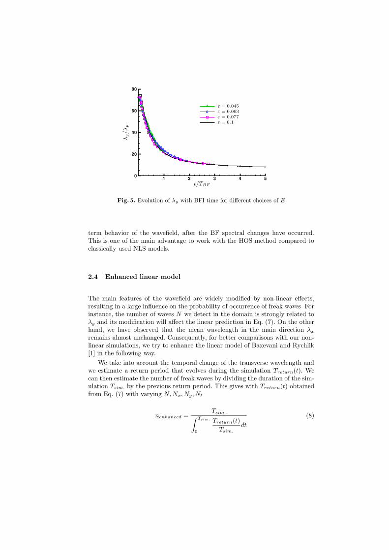
The most unstable directions with respect to the transverse Benjamin Feir(BF) instability (defined as ky = ±2−1/2kx) are also shown in Fig. 4. It clearlyappears that the spectral broadening occurs mainly along these directions. Thisemphasizes the influence of the BF mechanism in the spectrum evolution. Fig. 5presents the evolution of the measured mean transversal wavelength λy (nor-malized by peak wavenumber kp) versus normalized time t/TBF for differentsteepness ε where the BF time-scale TBF is defined as TBF = Tp ε

−2. We ob-serve that the curves for varied steepness all collapse together and a simple fitto the data would be λy(t) = λ(t = 0) exp [−t/TBF ].

The drastic reduction of the mean traversal wavelength is again related tothe BF mechanism as it is to be linked with the spectrum broadening. Note thatthe fully-non-linear HOS model gives access to times greater than TBF (duringwhich main changes occur in the spectrum) and therefore can predict the long

1 2 3 4 50

20

40

60

80

PSfrag replacementsλ

y/λ

p

t/TBF

ε = 0.01

ε = 0.032

ε = 0.045ε = 0.063ε = 0.077ε = 0.1

Fig. 5. Evolution of λy with BFI time for different choices of E

term behavior of the wavefield, after the BF spectral changes have occurred.This is one of the main advantage to work with the HOS method compared toclassically used NLS models.

2.4 Enhanced linear model

The main features of the wavefield are widely modified by non-linear effects,resulting in a large influence on the probability of occurrence of freak waves. Forinstance, the number of waves N we detect in the domain is strongly related toλy and its modification will affect the linear prediction in Eq. (7). On the otherhand, we have observed that the mean wavelength in the main direction λx

remains almost unchanged. Consequently, for better comparisons with our non-linear simulations, we try to enhance the linear model of Baxevani and Rychlik[1] in the following way.

We take into account the temporal change of the transverse wavelength andwe estimate a return period that evolves during the simulation Treturn(t). Wecan then estimate the number of freak waves by dividing the duration of the sim-ulation Tsim. by the previous return period. This gives with Treturn(t) obtainedfrom Eq. (7) with varying N,Nx, Ny, Nt

nenhanced =Tsim.∫ Tsim.

0

Treturn(t)

Tsim.dt

(8)

2.5 Discussion

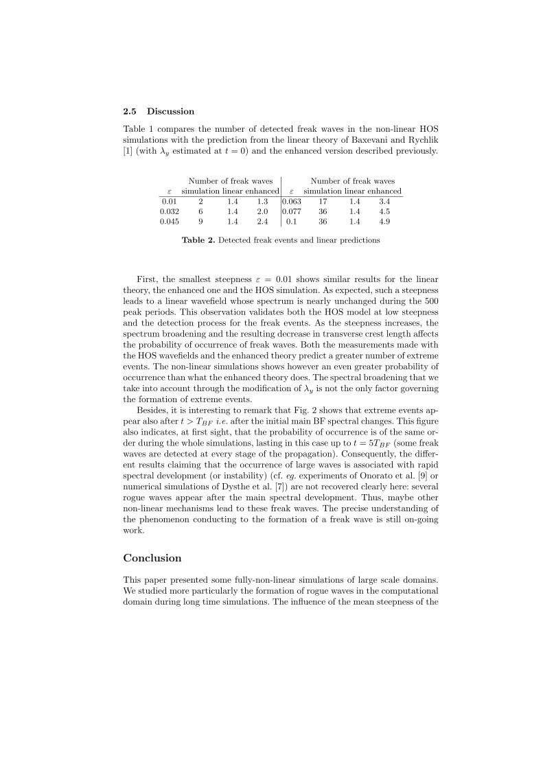
Table 1 compares the number of detected freak waves in the non-linear HOSsimulations with the prediction from the linear theory of Baxevani and Rychlik[1] (with λy estimated at t = 0) and the enhanced version described previously.

Number of freak waves Number of freak wavesε simulation linear enhanced ε simulation linear enhanced

0.01 2 1.4 1.3 0.063 17 1.4 3.40.032 6 1.4 2.0 0.077 36 1.4 4.50.045 9 1.4 2.4 0.1 36 1.4 4.9

Table 2. Detected freak events and linear predictions

First, the smallest steepness ε = 0.01 shows similar results for the lineartheory, the enhanced one and the HOS simulation. As expected, such a steepnessleads to a linear wavefield whose spectrum is nearly unchanged during the 500peak periods. This observation validates both the HOS model at low steepnessand the detection process for the freak events. As the steepness increases, thespectrum broadening and the resulting decrease in transverse crest length affectsthe probability of occurrence of freak waves. Both the measurements made withthe HOS wavefields and the enhanced theory predict a greater number of extremeevents. The non-linear simulations shows however an even greater probability ofoccurrence than what the enhanced theory does. The spectral broadening that wetake into account through the modification of λy is not the only factor governingthe formation of extreme events.

Besides, it is interesting to remark that Fig. 2 shows that extreme events ap-pear also after t > TBF i.e. after the initial main BF spectral changes. This figurealso indicates, at first sight, that the probability of occurrence is of the same or-der during the whole simulations, lasting in this case up to t = 5TBF (some freakwaves are detected at every stage of the propagation). Consequently, the differ-ent results claiming that the occurrence of large waves is associated with rapidspectral development (or instability) (cf. eg. experiments of Onorato et al. [9] ornumerical simulations of Dysthe et al. [7]) are not recovered clearly here: severalrogue waves appear after the main spectral development. Thus, maybe othernon-linear mechanisms lead to these freak waves. The precise understanding ofthe phenomenon conducting to the formation of a freak wave is still on-goingwork.

Conclusion

This paper presented some fully-non-linear simulations of large scale domains.We studied more particularly the formation of rogue waves in the computationaldomain during long time simulations. The influence of the mean steepness of the

wave field (or equivalently the BFI) on the freak waves occurrence probabilitiesis analysed.

Simulations are performed with the HOS method on a large domain (typically100 km2) during 500 Tp. The initial wave field is defined by a directional JON-SWAP spectrum and its fully-non-linear propagation during time is computed.Then, the wave pattern is analysed to detect freak waves appearing inside thedomain. In order to assess the correctness of our resolution, we take as referencethe work of Baxevani and Rychlik [1] which gives the probabilities of occurrenceof freak waves inside a domain during a period of time in a Gaussian (i.e. linear)framework. However, the non-linear evolution of the wave field induce severalchanges in the wave spectrum, particularly a spectral broadening with a peakdown-shifting. This has to be taken into account and consequently leads to anenhanced version of the linear prediction of Baxevani and Rychlik [1]. For thealmost linear case, both theories and HOS simulations are in concordance andassess the reliability of our fully-non-linear simulations as well as the methodof detection of freak events. Then, when the non-linearity of the wave field isenlarged, it appears clearly in the HOS simulations that the number of roguewaves observed is also widely increased and consequently greatly deviates fromthe linear theory. Furthermore, the enhanced linear theory predicts a correctincrease of this number of freak waves with the steepness but to a lesser extent.Thus, other non-linear effects than the spectral broadening are influent on theoccurrence of freak waves. Besides, our simulations indicate that extreme eventsappear also after t > TBF i.e. after the initial main BF spectral changes. Theunderstanding of the precise physical mechanisms leading to these freak waves(during and after the main spectral changes) is still under way and seems areally important point to clarify. Is there a long-time link between freak wavesformation and BF mechanism and/or what are the other non-linear mechanismsleading to such rogue waves ?

References

1. A. Baxevani and I. Rychlik. Maxima for gaussian seas. Ocean Engng., 33:895–911,2006.

2. I. I. Didenkulova, A. V. Slunyaev, E. N. Pelinovsky, and C. Kharif. Freak wavesin 2005. Nat. Hazards Earth Syst. Sci., 6:1007–1015, 2006.

3. D.G. Dommermuth. The initialization of nonlinear waves using an adjustmentscheme. Wave Motion, 32:307–317, 2000.

4. D.G. Dommermuth and D.K.P. Yue. A high-order spectral method for the studyof nonlinear gravity waves. J. Fluid Mech., 184:267 – 288, 1987.

5. G. Ducrozet, F. Bonnefoy, and P. Ferrant. Analysis of freak waves formation withlarge scale fully nonlinear high order spectral simulations. In Proc. 18th Int. Symp.on Offshore and Polar Engng., Vancouver, Canada, July 2008.

6. G. Ducrozet, F. Bonnefoy, D. Le Touze, and P. Ferrant. 3-D HOS simulations ofextreme waves in open seas. Nat. Hazards Earth Syst. Sci., 7(1):109–122, 2007.

7. K. Dysthe, H. Socquet-Juglard, K. Trulsen, H. E. Krogstad, and J. Liu. “Freak”waves and large-scale simulations of surface gravity waves. In Proc. 14th ‘AhaHuliko‘ a Hawaiian Winter Workshop, Honolulu, Hawaii, January 2005.

8. C. Kharif and E. Pelinovsky. Physical mechanisms of the rogue wave phenomenon.Eur. J. Mech., B/Fluids, 22:603–634, 2003.

9. M. Onorato, A.R. Osborne, M. Serio, L. Cavaleri, C. Brandini, and C.T. Stansberg.Extreme waves and modulational instability: wave flume experiments on irregularwaves. http://arxiv.org/abs/nlin.CD/0311031, 2004.

10. C. Guedes Soares, Z. Cherneva, and E.M. Antao. Characteristics of abnormalwaves in north sea storm sea states. Appl. Ocean Res., 25:337–344, 2003.

11. H. Socquet-Juglard, K. Dysthe, K. Trulsen, H. E. Krogstad, and J. Liu. Probabilitydistributions of surface gravity waves during spectral changes. J. Fluid Mech.,542:195–216, 2005.

12. M. Stiassnie and L. Shemer. On modifications of the zakharov equation for surfacegravity waves. J. Fluid Mech., 143:47–67, 1984.

13. K. Trulsen and K. B. Dysthe. A modified nonlinear schrdinger equation for broaderbandwidth gravity waves on deep water. Wave Motion, 24:281–289, 1996.

14. B.J. West, K.A. Brueckner, R.S. Janda, M. Milder, and R.L. Milton. A newnumerical method for surface hydrodynamics. J. Geophys. Res., 92:11803 – 11824,1987.

15. V. Zakharov. Stability of periodic waves of finite amplitude on the surface of adeep fluid. J. Appl. Mech. Tech. Phys., pages 190–194, 1968.