rock physics inversion: a montney case study 2012: vision 1 rock physics inversion: a montney case...

GeoConvention 2012: Vision 1

Rock Physics Inversion: A Montney Case Study

James Johnson, Schlumberger, Calgary, Alberta, Canada

[email protected]

and

Lisa Holmstrom, Murphy Oil Corporation, Calgary, Alberta, Canada

[email protected]

and

Satwant Diocee, Murphy Oil Corporation, Calgary, Alberta, Canada

[email protected]

and

Rob Tilson, Absolute Imaging, Calgary, Alberta, Canada

[email protected]

and

Sean Johnston, Schlumberger*, Calgary, Alberta, Canada

[email protected], *formerly, now with Taqa North Ltd.

Summary

In this case study, we applied a novel workflow for generating petrophysical property volumes in a Montney tight gas play. In the past, this method has been applied in high porosity, offshore oil exploration environments with great success (Westang et al, 2009). The workflow used involves the following steps:

a) Seismic data re-processing and conditioning

b) Log calibration and wavelet estimation

c) Low frequency model generation

d) Simultaneous pre-stack AVO inversion for elastic rock properties

e) Rock physics inversion for petrophysical properties

The AVO inversion algorithm is based on the Aki and Richards linear approximation to the Zoeprittz equations (Aki and Richards, 1980). The inversion is carried out simultaneously on multiple angle stacks in order to accurately derive elastic rock property volumes such as acoustic impedance, Vp/Vs ratio, and density.

The rock physics inversion is a new technique in characterizing tight gas plays. Initially, a rock physics model was developed relating the elastic rock properties to porosity, water saturation, volume of clay, volume of sand, and volume of carbonates using well logs and other available information. The model is consistent with the Reuss and Voigt bounds (Reuss, 1929), as well as Gassmann fluid substitution (Gassmann, 1951). The rock physics model is then used to define an inversion framework which is used to derive volumes of the above mentioned rock properties. The outputs of the rock physics inversion provide an intuitive laterally extensive characterization of reservoir quality, which may be of use in planning well placement and completions.

mailto:[email protected]

mailto:[email protected]


The quality of the results was evaluated by comparing the inversion results to the well log interpretations used to define the rock physics models, and also to other wells present in the study area that were not included in the analysis. The good match between the inversion and the well logs suggests the inversion results are reliable. Based on these results, the target zone of a Montney horizontal was altered. Once obtained the well logs confirmed this change in strategy.

Introduction

The Early Triassic Montney formation was deposited on the western margin of the North American Craton, and is divided into the Lower, Middle and Upper Montney all of which have slightly different characteristics. The Mineralogy of the Montney is best described as an arkosic siltstone with quartz, dolomite, and significant amounts of detrital K-Feldspar and Albite as the main framework grains. Calcite is present locally as shell fragments and is a common secondary mineral replacing framework grains. Grain-size is predominantly very-fine to coarse silts, but lower fine-grained sands occur in some areas. Overall the grain size increases from the Lower to Upper Montney, and from West to East in the same unit, however the mineralogy stays quite consistent. Total thickness of the formation is about 300 meters, and porosity ranges from 3 to 6 percent, and locally up to 9%. The Lower Montney was deposited in an offshore shelf environment and represents the down-dip equivalents of up-dip turbidites and more proximal shoreface successions consisting of finely laminated fine-grained siltstones associated with variable amounts of phosphate and pyrite. The progradation of the Lower Montney reached a maximum into the basin and is overlain by the Middle Montney, which consists of very fine-grained dark black arkosic siltstones associated with phosphate cements and nodules. Overlying this is the Upper Montney which developed as a series of prograding units out into the basin. The Upper Montney is composed of laminated fine-siltstone to fine-sand layers, with variable amounts of bioturbation.

This case study shows an AVO and rock physics inversion workflow applied to a Montney tight gas play. The inputs to the workflow are prestack seismic data, and well logs. As summarized above the inversion workflow consists of the following steps:

QC and loading of seismic and well log data

Log Calibration

Wavelet estimation

Low Frequency model building

Simultaneous AVO Inversion

AVO inversion yields elastic rock property volumes that are useful in reservoir characterization, and provide a better picture of lateral variation in reservoir quality then well logs alone can provide. Schlumberger’s ISIS inversion software uses a simulated annealing global optimization algorithm with a non linear cost function to optimize the results. This algorithm iteratively updates the modeled elastic rock properties, and forward models them using the Aki and Richards approximation to the zoeppritz equation to estimate subsurface reflectivity. This reflectivity model is then convolved with an estimated source signature to create modeled seismic data. As a part of the cost function the inversion algorithm seeks to minimize the misfit between the input and modeled seismic. The elastic properties used in this process are acoustic impedance, Vp/Vs ratio and density.

To gain a better understanding of the reservoir the AVO results are used as inputs in a subsequent, rock physics inversion. The rock physics inversion consists of three steps:


Model calibration

Additional low frequency model building

Rock physics inversion.

The rock physics inversion outputs are porosity, water saturation, and mineral fractions. The rock physics results provide an easy to interpret and intuitive measure of reservoir quality.

Method and Examples

AVO inversion requires high quality (i.e. true amplitude low noise no residual NMO) seismic data as an input to generate high quality results. To this end a novel noise reduction method was applied to the input seismic as part of an otherwise standard processing workflow. The data used is a fully reprocessed merge of 6 individual surveys, with a final bin spacing of 30 x 30 meters. Data quality is variable and degrades where thick gravel deposits exist near the surface.

Traditionally, the removal of random noise has been performed by using FX or FXY prediction filters (Canales, 1984). Recently more advanced methods using rank reduction have been introduced. Like FX filters, the rank reduction FX Singular Spectrum Analysis or Cadzow FX filter also uses matrices composed of complex valued Fourier coefficients, but instead of using a Weiner prediction filter with a least squares approximation the rank reduction method utilizes the singular value decomposition to generate a constant frequency slice matrix with a lower rank then the input. Cadzow filters can perform better than traditional FX filtering because the SVD rank reduction can be varied, making it more flexible. Cadzow is also better able to preserve the actual geological structures and random noise. Rank reduction methods also have the added advantage that they preserve amplitudes better than traditional FX/FXY methods and are therefore better suited to AVO.

The noise reduction algorithm was applied on cross-spreads prior to running PrSTM. Figure 1 below shows the input gathers before and after Cadzow filtering. Figure 2 shows inline sections with and without the noise reduction.

a) b)

Figure 1: Pre stack gathers a) before cadzow, b) after cadzow


a) b)

Figure 2: Inline section of PrSTM data a) without Cadzow b) with Cadzow noise reduction

After noise reduction the gathers were sorted into three angle stacks with angle ranges 5-15, 15-25 and 25-40 degrees. Figure 3 below shows an inline view of all 3 angle stacks. As shown by the plots, the quality of data in the area between xline 300 and 500 has been negatively affected by surface conditions.

a)


b)

c)

Figure 2: Inline section of post migration data a) without Cadzow b) with Cadzow noise reduction


Log calibration is the process of taking logs measured in depth and calibrating them to the time domain. This is done using the measured seismic velocities in the logs supplemented by visual ties. Log calibration and wavelet estimation are an iterative process. A calibrated log has its reflectivity calculated and convolved with a test wavelet to generate a synthetic seismic trace. This trace is then compared to the measured seismic trace. Once a good initial tie has been found a new wavelet can be estimated from the calculated reflectivity’s and measured seismic. Then further adjustments can be made to the well tie, which will lead to a new estimated wavelet. This process is carried out until a satisfactory match between the real and synthetic seismic is found.

In total eight wells were used in the project. Five of the wells had measured shear logs and were used in wavelet estimation and low frequency model building; the other three did not have measured shear logs, and were only used in low frequency model generation. For these wells synthetic shear logs were generated using petro physical analysis. Figure 4 below shows an outline of the survey area and spatial distribution of logs used.

Figure 4: Survey outline and well locations


The three wells not used in wavelet estimation, just low frequency model building, are 11-17, 15-8, B-43-9. These wells were calibrated using the wavelets estimated at the other wells. The final wavelet was estimated using the other five wells together. A time domain least squares method was used to try and match both the amplitude and phase of the input seismic at the location of all five wells over a ~300 ms TWT window in the zone of interest, in this case from the Halfway to the Belloy. A separate wavelet was estimated for each angle stack, and all 3 are shown in figure 5 below. Figure 6, shows the well tie for well 2-21, Figure 7 the same for 7-15.

Figure 5: Estimated Wavelets, Near is the 5-15 degree wavelet, mid the 15-25 degree wavelet, far the 25-30

degree wavelet

a) b) c)

Figure 6: Well tie for well 2-21 to a) the 5-15 degree angle stack, b) the 15-25 degree angle stack c) the 25-40 degree angle stack. The red line is the acoustic impedance calculated from the logs, calibrated in time.


a) b) c)

Figure 7: Well tie for well 7-15 to a) the 5-15 degree angle stack, b) the 15-25 degree angle stack c) the 25-40 degree angle stack.

The average cross correlation of the measured and synthetic seismic for the wells used in wavelet estimation is 0.77 for the near stack, 0.80 for the mid stack and 0.74 for the far stack. The blue and green arrows in figures 6 and 7 show the window over which the wavelet was estimated and the cross correlation was calculated.

Due to the band limited nature of seismic data the inversion algorithm requires an a priori, low frequency model, to produce absolute valued results. We generated the model by laterally extrapolating well data to cover the whole survey area. The extrapolation was constrained by horizons picked on the input seismic. In this case the Halfway, Belloy, and two other surfaces in between them were used. Prior to lateral extrapolation the wells logs were low pass filtered so they only fill in the low frequency information not present in the seismic data. The weight given to the data from each well was inversely proportional to the square of the offset distance from the well. Figure 8 below shows logs for all 8 wells used in building the low frequency model, as if they were all at the same location (that of 7-15 in this case). This plot was made by stretching/squeezing the section of log between each horizon so that they cover the same TWT. This plot is useful in determining any lateral variations or depth trends present in the area of interest. Figure 8 shows that the wells in question largely agree until just above the Belloy.


a) b) c)

Figure 8: Logcrossvallidation plots, a) acoustic impedance, b) vp/vs ratio c) density. The plots on the left are the calibrated logs, the plots on the right are the low pass filtered calibrated logs used in LFM building.

The next step in the workflow is the actual 3D simultaneous AVO inversion, which has three main outputs, acoustic impedance, Vp/Vs ratio and density. The inputs are the previously mentioned angle stacks, wavelets and low frequency models.

The inversion algorithm expressed mathematically is:

As mentioned above a simulated annealing algorithm is used to find a set of Zp ‘s that minimize the various penalty functions (E equations).The p superscripts denote the various mechanical properties modeled, while the s subscripts denote the different angle stacks used. The w terms represent weight factors given to the different penalty functions, and are controlled by the user. Eseismic is the misfit of the input (ds) and synthetic seismic, here w(t) represents the wavelets, and r the reflectivity calculated from the Zp ‘s using Aki and Richards approximation to zoepritz equation (Aki and Richards 1980). Eprior is the misfit between the modeled properties and the low frequency models. Ehorizontal is a continuity term


which controls the amount of lateral variation present in the output data. Evertical contains a threshold ro which is set by the user. This term is used to control the number of significant reflectors which are modeled.

Figures 9-11 show the results for several of the wells used in the project. In figures 9-11 the green curve is the low frequency model, the blue curve the inversion result along the path of the well, and red curve is the well log. The well logs were low pass filtered with a cutoff of 90 hertz to compare them to the inversion results which are limited by the seismic bandwidth.

a) b) c)

Figure 9: Inversion results at well 2-21 for a) acoustic impedance, b) Vp/Vs ratio c) density

a) b) c)

Figure10: Inversion results at well 7-15 for a) acoustic impedance, b) Vp/Vs ratio c) density


a) b) c)

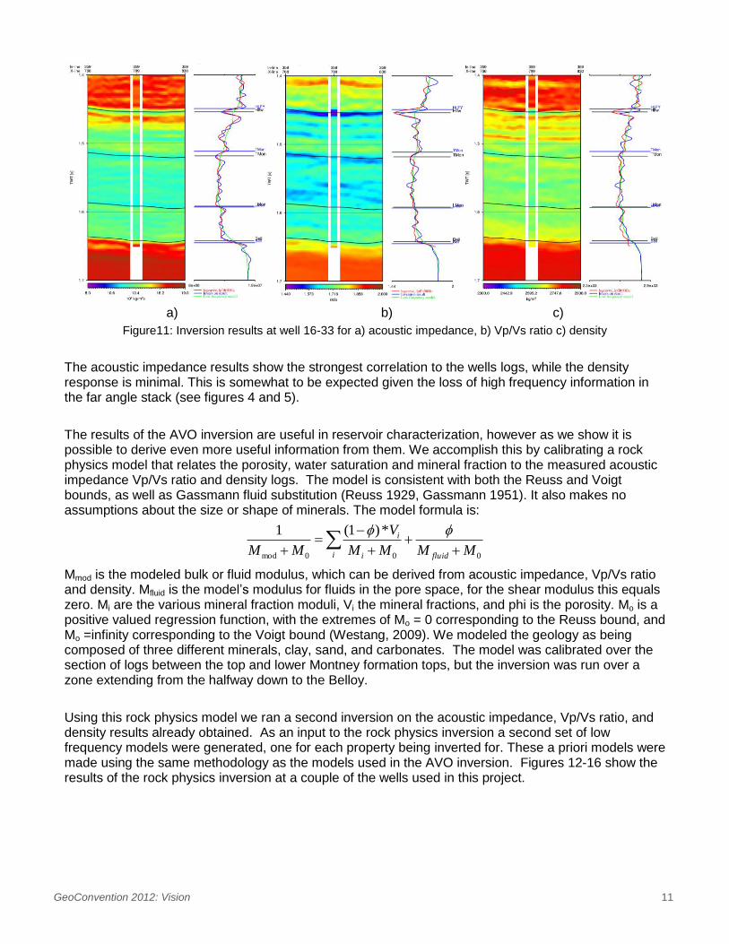
Figure11: Inversion results at well 16-33 for a) acoustic impedance, b) Vp/Vs ratio c) density

The acoustic impedance results show the strongest correlation to the wells logs, while the density response is minimal. This is somewhat to be expected given the loss of high frequency information in the far angle stack (see figures 4 and 5).

The results of the AVO inversion are useful in reservoir characterization, however as we show it is possible to derive even more useful information from them. We accomplish this by calibrating a rock physics model that relates the porosity, water saturation and mineral fraction to the measured acoustic impedance Vp/Vs ratio and density logs. The model is consistent with both the Reuss and Voigt bounds, as well as Gassmann fluid substitution (Reuss 1929, Gassmann 1951). It also makes no assumptions about the size or shape of minerals. The model formula is:

000mod

*)1(1

MMMM

V

MM fluidi i

i

Mmod is the modeled bulk or fluid modulus, which can be derived from acoustic impedance, Vp/Vs ratio and density. Mfluid is the model’s modulus for fluids in the pore space, for the shear modulus this equals zero. Mi are the various mineral fraction moduli, Vi the mineral fractions, and phi is the porosity. Mo is a positive valued regression function, with the extremes of Mo = 0 corresponding to the Reuss bound, and Mo =infinity corresponding to the Voigt bound (Westang, 2009). We modeled the geology as being composed of three different minerals, clay, sand, and carbonates. The model was calibrated over the section of logs between the top and lower Montney formation tops, but the inversion was run over a zone extending from the halfway down to the Belloy.

Using this rock physics model we ran a second inversion on the acoustic impedance, Vp/Vs ratio, and density results already obtained. As an input to the rock physics inversion a second set of low frequency models were generated, one for each property being inverted for. These a priori models were made using the same methodology as the models used in the AVO inversion. Figures 12-16 show the results of the rock physics inversion at a couple of the wells used in this project.


a) b) c)

Figure 12: Porosity inversion results at a) well 7-15 b) 2-21 c) 16-1

a) b) c)

Figure 13: Water saturation inversion results at a) well 7-15 b) 2-21 c) 16-1

a) b) c)

Figure 14: Volume of clay inversion results at a) well 7-15 b) 2-21 c) 16-1


a) b) c)

Figure 15: Volume of sand inversion results at a) well 7-15 b) 2-21 c) 16-1

a) b) c)

Figure 16: Volume of carbonates inversion results at a) well 7-15 b) 2-21 c) 16-1

As a test, a well not used in either the low frequency model building or wavelet estimation was calibrated to the time domain, and then compared with the inversion results. Figure 17 shows the location of the blind test well 13-14. Figure 18 shows the results of the AVO inversion, while figure 19 the rock physics inversion results. We believe that the strong correlation between this blind well and our inversion, especially for acoustic impedance and porosity show the accuracy of our method in predicting subsurface rock properties.


Figure 17: Location of blind test well

a) b) c)

Figure 18: AVO inversion results at blind test well 13-14, a) acoustic impedance b) Vp/Vs ratio c) density


a) b) c)

e) f)

Figure 19: Rock physics inversion results at well 13-14 a) porosity b) water saturation c) volume of clay d) volume of sand e) volume of carbonates

Based on the rock physics inversion results the target zone of an additional well was altered, and once obtained the well logs confirmed this choice. Figure 20 below shows the AVO results at this new well, and figure 21 shows the rock physics results.


a) b) c)

Figure 20: AVO inversion results compared to logs from well drilled based on them a) Acoustic impedance b) Vp/Vs ratio c) density

a) b) c)

e) f)

Figure 20: Rock physics inversion results compared to logs from well drilled based on them a) Porosity b) Water saturtion c) Volume Clay d) Volume sand e) Volume carbonates


Conclusions

We have demonstrated a novel workflow for taking prestack seismic data through AVO inversions, and a second rock physics inversion. The AVO inversion uses the Aki and Richards linear approximation to the Zoeppritz equations. The rock physics model used is consistent with Reuss and Voigt bounds, as well as Gassmann fluid substitution. We showed the accuracy of the results against a blind well not used in the model calibration. Based on these results the location of a horizontal well was altered, and once drilled the well logs confirmed this decision.

Acknowledgements

We would like to thank Murphy Oil Corporation for allowing us to publish this case study, as well as Kjetil Westang, Henrik Juhl Hansen, and Klaus Bolding Rasmussen for their work developing the rock physics inversion software.

References

Westang, K., Hansen, H., Rasmussen, K., 2009, ISIS Rock Physics – a new petro-elastic model for optimal rock physics inversion with

examples from the Nini field: University of Bergen, Sound of Geology Workshop 2009

Gassmann, F., 1951, Elasticity of Porous Media, Veirteljahrsschrift der Naturfshenden Gesellschaft, Zurich, 96, 1-23

Reuss, A., 1929, Berechung der fliessgrense von mischkristallen auf grund der plastizitatbedinggun fur einkristalle. Zeitschrift fur

An’ewandte Mathematik und Mechanik, 9, 49-58

Aki, K., Richards, P., 1980, Quantitative Seismology, Theory and Methods, Vol I, 5.2

Canales, L.L., 1984, Random noise reduction: 54th Ann. Internat. Mtg., SEG Expanded abstracts, 525-527

Zoeppritz, K., 1919, Erdbebenwellen VII. VIIb. Über Reflexion und Durchgang seismischer Wellen durch Unstetigkeitsflächen.

Nachrichten von der Königlichen Gesellschaft der Wissenschaften zu Göttingen, Mathematisch-physikalische Klasse, 66-84.

rock physics inversion: a montney case study 2012: vision 1 rock physics inversion: a montney case...

Documents