rock particle image segmentation and systemscdn.intechweb.org/pdfs/5786.pdf · rock particle image...

8

Rock Particle Image Segmentation and Systems

Weixing Wang Collage of Computer Science and Technology, Hubei University of Technology,

Wuhan, Hubei,

China

1. Introduction

As known, most important, and the hard part of pattern recognition for rock particles, is image

segmentation. Segmentation can be divided into two steps, one is segmentation based on gray

levels (called image binarization, sometimes) in which a gray level image is processed and

converted into a binary image. Another is segmentation based on rock particle shapes in a

binary image, in which overlapping and touching particles will be split, and over-segmented

particles will be merged based on some prior knowledge such as shape and size etc.

Segmentation algorithms for monochrome (gray level) images generally are based on one of

two basic properties of gray-level values: similarity and discontinuity. The principal

approaches in the first category are based on thresholding, region growing, and region

splitting and merging. In the second category, the approach is to partition an image based

on abrupt changes in gray level. The principal areas of interest within this category are

detection of isolated points and detection of lines and edges in an image.

The choice of segmentation of rock particle images based on similarity or discontinuity of

the gray-level values depends on both developed sub-algorithms and applications.

Rock particle images have their own characteristics compared to other particle images.

Generally speaking, under the frontlighting illumination condition which is common case,

rock particle images have the characteristics: (1) uneven background and foreground for

which a simple thresholding algorithm cannot be applied to segment the images; (2) each

rock particle may possess a textured surface and multiple faces, which often causes an over-

segmentation problem; (3) rock particle overlapping each other, which hides parts of a

particle, or causes breaks of the boundaries of rock particles; (4) touching rock particles

forming a large cluster; (5) rain, snow, or much fine material making rock particle images

clump together.

Rock particles may be densely packed or be separated mostly on a background. The former

case is more difficult to process than the latter. As well known, most systems for rock

particle images were developed based on simple thresholding algorithms (some of them

combined with morphological segmentation algorithm) and boundary detection algorithms.

The segmentation algorithm designing is application (here, the type of rock particle images)

dependent. In this chapter, the author summarize own segmentation approaches for rock

particle images, they are: (1) an algorithm based on edge detection; (2) an algorithm based

on region split-and-merge; (3) an adaptive thresholding algorithm; and (4) an algorithm for

splitting touching particles in a binary image. Ope

n A

cces

s D

atab

ase

ww

w.i-

tech

onlin

e.co

m

Source: Pattern Recognition Techniques, Technology and Applications, Book edited by: Peng-Yeng Yin, ISBN 978-953-7619-24-4, pp. 626, November 2008, I-Tech, Vienna, Austria

www.intechopen.com

Pattern Recognition Techniques, Technology and Applications

198

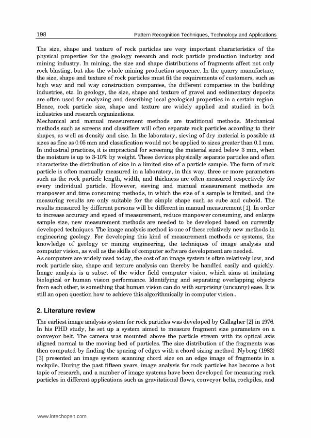
The size, shape and texture of rock particles are very important characteristics of the

physical properties for the geology research and rock particle production industry and

mining industry. In mining, the size and shape distributions of fragments affect not only

rock blasting, but also the whole mining production sequence. In the quarry manufacture,

the size, shape and texture of rock particles must fit the requirements of customers, such as

high way and rail way construction companies, the different companies in the building

industries, etc. In geology, the size, shape and texture of gravel and sedimentary deposits

are often used for analyzing and describing local geological properties in a certain region.

Hence, rock particle size, shape and texture are widely applied and studied in both

industries and research organizations.

Mechanical and manual measurement methods are traditional methods. Mechanical

methods such as screens and classifiers will often separate rock particles according to their

shapes, as well as density and size. In the laboratory, sieving of dry material is possible at

sizes as fine as 0.05 mm and classification would not be applied to sizes greater than 0.1 mm.

In industrial practices, it is impractical for screening the material sized below 3 mm, when

the moisture is up to 3-10% by weight. These devices physically separate particles and often

characterize the distribution of size in a limited size of a particle sample. The form of rock

particle is often manually measured in a laboratory, in this way, three or more parameters

such as the rock particle length, width, and thickness are often measured respectively for

every individual particle. However, sieving and manual measurement methods are

manpower and time consuming methods, in which the size of a sample is limited, and the

measuring results are only suitable for the simple shape such as cube and cuboid. The

results measured by different persons will be different in manual measurement [1]. In order

to increase accuracy and speed of measurement, reduce manpower consuming, and enlarge

sample size, new measurement methods are needed to be developed based on currently

developed techniques. The image analysis method is one of these relatively new methods in

engineering geology. For developing this kind of measurement methods or systems, the

knowledge of geology or mining engineering, the techniques of image analysis and

computer vision, as well as the skills of computer software development are needed.

As computers are widely used today, the cost of an image system is often relatively low, and

rock particle size, shape and texture analysis can thereby be handled easily and quickly.

Image analysis is a subset of the wider field computer vision, which aims at imitating

biological or human vision performance. Identifying and separating overlapping objects

from each other, is something that human vision can do with surprising (uncanny) ease. It is

still an open question how to achieve this algorithmically in computer vision..

2. Literature review

The earliest image analysis system for rock particles was developed by Gallagher [2] in 1976.

In his PHD study, he set up a system aimed to measure fragment size parameters on a

conveyor belt. The camera was mounted above the particle stream with its optical axis

aligned normal to the moving bed of particles. The size distribution of the fragments was

then computed by finding the spacing of edges with a chord sizing method. Nyberg (1982)

[3] presented an image system scanning chord size on an edge image of fragments in a

rockpile. During the past fifteen years, image analysis for rock particles has become a hot

topic of research, and a number of image systems have been developed for measuring rock

particles in different applications such as gravitational flows, conveyor belts, rockpiles, and

www.intechopen.com


199

laboratories, and some of them are under development. The researches and developments

have been and are carried out in many countries such as Sweden, Germany, France,

England, Australia, Canada, United States, China, South Africa, and Spain etc.[4-11]. Generally speaking, a system consists of three parts: image acquisition, image segmentation

and particle size and shape measurement. Image acquisition is about how to set up an image

acquisition system to acquire rock particle images of good quality under different work

conditions, which is often strongly application dependent. Image segmentation is an

important part in the whole system. The design of an image segmentation algorithm

depends on the characteristics of rock particle images. The image segmentation results affect

the accuracy of measurement of size, shape and texture of rock particle particles. The basic

requirement for size, shape and texture measurement is that the measurement results

should be reproducible, and should reflect as much information as possible.

According to algorithms or methods of image segmentation, the existing systems could be

classified into at least four classes. They are: (1) thresholding on histogram of gray levels [12-

18]; (2) boundary tracing or edge detection [2-3, 7-8, 19-33]; (3) region growing or merge &

split [9-10, 34-37]; and (4) thresholding and granulometry (= morphology segmentation on a

binary image) [38-41]. Systems based on thresholding of histogram of gray levels were applied in some

applications in which rock particle images have a uniform background, and rock particle

possessing less surface texture. The typical application is measuring rock particles in a

gravitational flow. Recently, such systems are used both in laboratories and for conveyor

belts in the field [15-18]. The system uses backlighting illumination (a special lighting

condition is constructed) to acquire rock particle images from a free falling rock particle

stream, the acquired images being almost binarised ones. Therefore, a simple threshold can

separate rock particles and background easily.

There is a number of systems developed based on boundary tracing or edge detection

algorithms. The early systems mentioned before [2-3], used a difference operator to obtain a

gradient magnitude image from a gray level image, then binarised the gradient magnitude

image. The binarised image is the image with contours of particles. In most cases, the

segmentation results are not satisfactory due to the fact that the contours of particles are not

closed curves, and false edges exist. In order to overcome the problems, some recent systems

include procedures (sub-algorithms) for gap linking, false edge elimination and curve

closing. Some typical examples are summarized below.

In Lin, Yen and Miller’s system (1995) [31], an image of overlapped rock fragments, taken

from a moving conveyor belt, is first smoothed with an edge preserving filter, secondly

detected by an edge detection operator (Canny’s algorithm), then processed by edge linking

and edge gap filling, finally followed by segment connection. Transforming the intensity

function of the processed image for the desired intensity regions smooths the original image.

The Canny edge detector is used with a so-called hysteresis thresholding algorithm to

extract edges from the smoothed image. Supplementary to edge detection, edge linking and

gap filling functions are added in the algorithm.

Kemeny et al. [24-27] system has been used in many cases. The system enhances an image

by equalizing histogram of gray levels, then thresholds the enhanced image to separate void

spaces among particles (non-particle regions), so-called shadows, from particles. Meanwhile

a gradient magnitude image is obtained by using a Sobel difference operator. Particles are

delineated by searching for large gradient paths ahead of sharp convexities of the shadows

www.intechopen.com


200

to separate clusters of touching rock particles. Using a morphological segmentation

algorithm splits the remaining touching particles.

Norbert, Tom and Franklin [21-22 setup a system since 1988]: The work sequence of the

segmentation algorithm is similar to Kemeny’s one. It includes two steps. The first step is to

segment particles by use of several conventional image processing techniques, including the

use of thresholding and gradient operators. In this step, the faint shadows between adjacent

particles are detected, and the work step is available for clean images with lightly textured

rock surfaces. The second step uses a number of reconstruction techniques to further

delineate particles which are only partly outlined during the first step. In the second step,

the algorithm is just for closing particle contours. Bedair 1996 in his Ph.D. study, developed

a similar particle contour closing algorithm, the detail description can be found in [32-33].

In morphological segmentation of rock particle images, the thresholded binary image is the

objective. Two kinds of algorithms have been used in the image analysis systems for rock

particles: one is granulometry, the other is Watershed algorithm.

The general idea of the Granulometry algorithm is that in order to simulate the sieving

analysis, one can generate a series of squares (a maximum square inside of an particle) to

obtain size distribution. In this algorithm, the complex segmentation is avoided. The ideal

case is that particles have some regular shape (e.g. circle, square, or diamond). It is mainly

based on the functions of opening and closing with a certain structure element, and distance

transformation. The systems applying the algorithm can be found in [39-41].

Yen, Lin and Miller’s method (1994) [38] - a derivative of the Watershed segmentation: It

includes seven steps: (1) “Edge Preserving Smoothing” technique is applied to the

overlapped fragment image to eliminate the fluctuation of highs and lows on the particle

surface as much as possible but preserve the edge points; (2) the Sobel edge detector is used

to find the edges on the smoothed particle image; (3) A median filter is utilized to eliminate

the noise on the edge image; (4) the smoothed edge image is subtracted from the original

image to construct an “edge cutted” (EC) image; (5) a gray scale morphology erosion is

applied to shrink EC particle image to an extent such that no overlap occurs; (6) the “Otsu”

thresholding algorithm [74] is used to shrunk, non-overlapped image and a labeling

procedure used to identify each mark; (7) Once these inside markers have been located the

“Odered Queue Watershed” algorithm can then be applied to the original particle image to

separate the overlapped particles. The segmentation result is not very satisfactory even to

well sorted particles with a good background.

The segmentation algorithms of region growing or merge & split for rock particle images [9-

10, 34-37] were and are mainly developed by the author. The chapter will discuss that

segmentation algorithm. All the four kinds of segmentation algorithms have been

developed more or less in the study. The different developed algorithms have been chosen

for different applications. The developed algorithms are described and compared too.

3. Image segmentation algorithm for rock particles

As mentioned before, most important, and the hard part of computer vision for rock particles,

is segmentation. Segmentation can be divided into two steps, one is segmentation based on

gray levels (called image binarization, sometimes) in which a gray level image is processed

and converted into a binary image. Another is segmentation based on particle shapes in a

binary image, in which overlapping and touching particles will be split, and oversegmented

particles will be merged based on some prior knowledge such as shape and size etc.

www.intechopen.com


201

3.1 The algorithms based on edge detection 3.1.1 Crucial algorithm edge detection As most developed segmentation algorithms in the existing systems for rock particle images, an algorithm based on edge detection was also developed in this study. The main parts of the algorithm are (1) image smoothing; (2) edge detection by an edge operator; (3) thresholding on the obtained gradient magnitude image; and (4) noise edge deleting and edge gap linking. After image smoothing (e.g. Gaussian smoothing), the Canny edge detector [59] is applied on the smoothed image. The gradient magnitude image obtained by Canny’s operator, is thresholded by the P-tile thresholding algorithm, the value of the P-tile is chosen according to characteristics of rock particle images. Before noise edges deleting and edge gap linking, the thresholded image is thinned by a thinning function. After this operation, all the end points of edges (lines or curves) are detected, and small gaps between two edges are linked, where some end points disappear. All the edges of the end points are eroded from the end

points within a certain length LE(a number of pixels), the short edges of length < LE, are removed. The remaining edges are then dilated to recover their original states. Finally, the gaps (e.g. the length of a gap is less than 20 pixels) between edges are linked. As examples, two densely packed rock particle images are segmented by the algorithm (see Fig. 1). In the present stage, the algorithm can not provide closed curve for each individual particle, but the segmentation result can be used for estimation of average size of densely packed rock particle particles.

(a) (b) (c)

(d) (e) (f) Fig. 1. Segmentation based on edge detection. (a) Original image #1. (b) Image after Canny operation on (a). (c) Image after deleting noise edges and gap linking on (b). (d) Original image #2. (e) Image after Canny operation on (d). (f) Image after noise edges deleting and gap linking on (e).

www.intechopen.com


202

3.1.2 The algorithm of one-pass boundary detection The goal of edge detection in our case is to quickly and clearly detect the boundaries of particles, it is not necessary to close every particle’s boundary (it is too hard), but it should produce less gaps on boundaries and less noise edges on the particles. To reach this goal, we tested several widely used edge detection algorithms for a typical particle image; in Fig. 2, (a) original image (150x240x8 bits), (b) Sobel edge detection result that includes too much

white noise, (c) Robert edge detection result that is mass, (d) Laplacian edge detection result that miss boundaries much, (e) Prewitt edge detection result that is similar to (a), (f) and (g) Canny edge detection results which are thresholding value dependent, and (h) the result from our developed one-pass boundary detection algorithm. By comparing results from the seven tests, the new algorithm gives the best edge (boundary) detection result. Our algorithm [53] is actually a kind of ridge detector (or line detector).

(a) (b) (c) (d)

(e) (f) (g) (h)

Fig. 2. Testing of edge detection algorithms: (a) Original image; (b) Sobel detection; (c)

Robert detection; (d) Laplacian detection; (e) Prewitt detection; (f) Canny detection with a

high threshold; (g) Canny detection with a low threshold; and (h) Boundary detection result

by the new algorithm.

To overcome the disadvantages of the above first six edge detection algorithms, we studied a

new boundary detection algorithm (Fig. 2 (h)) based on ridge (or valley) information. We use the

word valley as an abbreviation of negative ridge. The algorithm is briefly described as follows:

A simple edge detector uses differences in two directions: ( ) ( )1, ,x

f x y f x yΔ = + −

and ( ) ( ), 1 ,y

f x y f x yΔ = + − , where ( ),f x y is a grey scale image.

www.intechopen.com


203

In our valley detector, we use four directions. Obviously, in many situations, the horizontal

and vertical grey value differences do not characterize a point, such as P (in Fig. 3), well.

Fig. 3. Examine the point P, determining if it is a valley pixel, or not. Circles in the sparse (i,

j)-grid. It moves for each P ∈ (x, y)-grid. (a) A grey value landscape over layered with a

sample point grid. (b) PA-PB section.

In Fig. 3, we see that P is surrounded by strong negative and positive differences in the

diagonal directions:

450∇ < , and

450Δ > ,

1350∇ < , and

1350Δ > , whereas,

00∇ ≈ , and

00Δ ≥ ,

900∇ ≈ , and

900Δ ≈ , where Δ are forward differences: ( ) ( )45

1, 1 ,f i j f i jΔ = + + − , and ∇ are

backward differences: ( ) ( )45, 1, 1f i j f i j∇ = − − − etc. for other directions. We use

( )max α αΔ −∇ as a measure of the strength of an edge point. It should be noted that we use

sampled grid coordinates, which are much more sparse than the pixel grid 0 x n≤ ≤ ,

0 y m≤ ≤ . f is the original gray value image after slight smoothing.

What should be stressed about the valley edge detector is:

a. It uses four instead of two directions;

b. It studies value differences of well separated points: the sparse 1i ± corresponds to

x L± and 1j ± corresponds to y L± , where 1L >> , in our case, 3 7L≤ ≤ . In

applications, if there are closely packed particles of area > 400 pixels, images should be

shrunk to be suitable for this choice of L. Section 3 deals with average size estimation,

which can guide choice of L;

www.intechopen.com


204

c. It is nonlinear: only the most valley-like directional response ( )α αΔ −∇ is used. By

valley-like, we mean ( )α αΔ −∇ value. To manage valley detection in cases of broader

valleys, there is a slight modification whereby weighted averages of ( )α αΔ −∇ -

expressions are used.

( ) ( ) ( ) ( )1 2 2 1B A B Aw P w P w P w Pα α α αΔ + Δ − ∇ − ∇ , where,

AP and

BP are shown in Fig. 3.

For example, w1=2 and w2=3 are in our experiments.

d. It is one-pass edge detection algorithm; the detected image is a binary image, no need

for further thresholding.

e. Since each edge point is detected through four different directions, hence in the local

part, edge width is one pixel wide (if average particle area is greater than 200 pixels, a

thinning operation follows boundary detection operation);

f. It is not sensitive to illumination variations, as shown in Fig. 4, an egg sequence image.

On the image, illumination (or egg color) varies from place to place, for which, some

traditional edge detectors (Sobel and Canny etc.) are sensitive, but the new edge

detector can give a stable and clear edge detection result comparable to manual

drawing result.

The algorithm has been tested for a number of images. It works satisfactory in several kinds

of applications, and the testing results are shown in Figs. 5 -8.

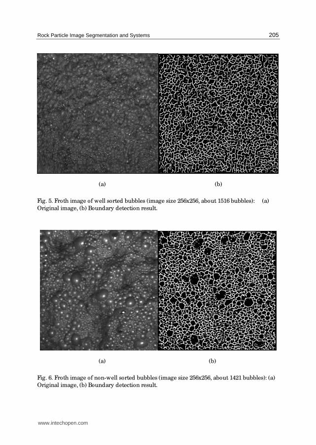
In Fig. 5, the froth is very small, say, 43 pixels per bubble on average, it is hard to delineate

by using a common image segmentation algorithm.

The image in Fig. 6 is different from the image in Fig. 5: the bubble size varies much; the

white spots can clearly be seen on relative large bubbles. The ordinary edge detector may

just detect the edges of the white spots, which are not the boundaries of the bubbles.

The image in Fig. 7 includes a mass of rough surface particles (average area is about 45

pixels), the new algorithm works well even for this kind of images.

(a) (b) (c)

(d) (e) (f)

Fig. 4. Egg image test: (a) original image (400x200 pixels), (b) new algorithm result, (c)

manual drawing result (180 eggs), (d) Sobel edge detection result, and (e) and (f) Canny

edge detection results with different thresholds.

www.intechopen.com


205

(a) (b)

Fig. 5. Froth image of well sorted bubbles (image size 256x256, about 1516 bubbles): (a)

Original image, (b) Boundary detection result.

(a) (b)

Fig. 6. Froth image of non-well sorted bubbles (image size 256x256, about 1421 bubbles): (a)

Original image, (b) Boundary detection result.

www.intechopen.com


206

(a) (b)

Fig. 7. Soil image of well sorted particles (image size 256x256, about 1445 particles): (a)

Original image (particle surface is very rough), (b) Boundary detection result.

In Fig. 8, the image consists of a number of crushed aggregate particles, 47 pixels per

aggregate particle on average. Even for the non-smooth (non-rounded) surface particles, the

new edge detection algorithm can give a good detection result.

(a) (b)

Fig. 8. Crushed aggregate image of well sorted particles (image size 356x288, about 2173

particles): (a) Original image, (b) Boundary detection result.

www.intechopen.com


207

The new algorithm includes only some kind of differentiation - one of the three operations

(differentiation, smoothing and labeling) by comparing to ordinary edge detectors. It is a

kind of line detection algorithm, but detecting lines in four directions.

After boundary detection, the edge density will be counted and converted to particle size,

the next section presents our particle size estimation algorithm.

3.2 The algorithm based on split-and-merge For the images of densely packed rock particle particles, the above segmentation algorithm

can provide average size rather than size distribution of particles. To meet the requirement

of obtaining a size distribution of rock particle particles, a segmentation algorithm based on

region split-and-merge was developed. The algorithm consists of three parts: (1) Suk &

Chung algorithm-Single-pass split-and-merge [60]; (2) merging small regions into their

adjacent large regions; (3) background split and regions merge based on shape of rock

particle particles.

For a rock particle image, the Suk & Chung algorithm [60] is first applied to segment the

rock particle image into small regions. However, this segmentation based on gray values,

yields a number of the small regions amounting to tens up to hundreds times the real

number of particles in an image. In order to reduce the number of the small regions, a merge

procedure was developed, in which the two steps are included: (1) Find the small regions Rs

(< T3, T3 is a threshold value); (2) Among Rj (j =1,2, ...), all the neighboring regions of Rs ,

find Rm (j = m) for which the common edges between Rs and Rj is maximal, and then merge

Rs and Rm.

Sometimes, the whole rock particle image is not fully occupied by the particles. Parts of the

non-particles regions or void spaces tend to be dark. To eliminate regions belonging to dark

background, one may let regions of average gray value below a pre-defined threshold be re-

classified as background, so-called "background split". The use of a pre-defined threshold is

partly enabled by the normalization pre-processing procedure.

When the background is split from the image (i.e. the image is converted into a binary

image), over-segmentation problem still exists in the binarized image. To overcome this

problem, a procedure for merging regions based on shape of rock particle particles was

constructed. In the merge procedure, three basic merge criteria were considered for two

neighboring regions (or objects), they are: (1) their common boundary length is relatively

long; (2) the gray value difference between two objects is not too large; and (3) if two objects

are merged, the two junction points should not be concave points.

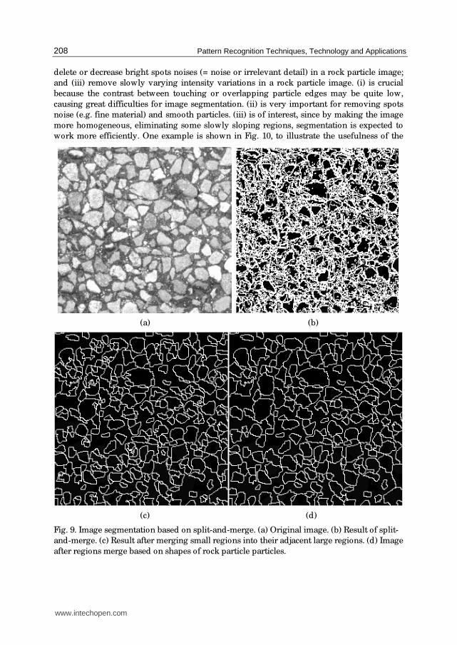
The whole algorithm work sequence is illustrated in the following Figures. An original rock

particle image (from pavement) is shown in Fig. 9(a). In the first processing step, the image

is merged and split into many small regions, each of them has an uniform gray intensity (see

Fig. 9(b)). After merging small regions into their adjacent large regions, the result image is

shown in Fig. 9(c), where the over-segmentation problem still exists. To reduce this kind of

problem, in the last step, the merge procedure on a binary image, is used, and the result is

shown in Fig. 9(d).

When a rock particle image is complex as shown in Fig. 10(a), one extra pre-processing

algorithm has to be used before the segmentation algorithm is applied. The image pre-

processing algorithm was designed to: (i) strengthen the edges among the rock particles; (ii)

www.intechopen.com


208

delete or decrease bright spots noises (= noise or irrelevant detail) in a rock particle image;

and (iii) remove slowly varying intensity variations in a rock particle image. (i) is crucial

because the contrast between touching or overlapping particle edges may be quite low,

causing great difficulties for image segmentation. (ii) is very important for removing spots

noise (e.g. fine material) and smooth particles. (iii) is of interest, since by making the image

more homogeneous, eliminating some slowly sloping regions, segmentation is expected to

work more efficiently. One example is shown in Fig. 10, to illustrate the usefulness of the

(a) (b)

(c) (d)

Fig. 9. Image segmentation based on split-and-merge. (a) Original image. (b) Result of split-

and-merge. (c) Result after merging small regions into their adjacent large regions. (d) Image

after regions merge based on shapes of rock particle particles.

www.intechopen.com


209

image pre-processing algorithm. The segmentation result is not satisfactory because of

without using the preprocessing procedure before segment the image.

(a) (b)

(c) (d)

Fig. 10. Comparison between two segmentation results by using the segmentation algorithm

described in the following section. (a) Original image. (b) Image after the pre-processing. (c)

Segmented result on the image in (a). (d) Segmented result on the image in (b).

Before the above procedure, a preprocessing step is operated. as the follows.

The principal objective of image pre-processing is to process an image so that the result is

more suitable than the original image for a specific segmentation algorithm. For the ceramic

surface image segmentation, in order to make images more suitable for segmentation, we

use our pre-processing program to reduce image noises in three steps: (1) strengthen the

www.intechopen.com


210

edges among the ceramic grains; (2) delete or decrease bright spots noises (= noise or

irrelevant detail) in a ceramic image, and (3) remove slowly varying intensity variations in a

ceramic image. Item (1) is crucial because the contrast between touching or overlapping

grain edges may be quite low, causing great difficulties for image segmentation. Item (2) we

have already discussed. Item (3) is of interest, since by making the image more

homogeneous, eliminating some slowly sloping regions, segmentation is expected to work

more efficiently.

We strengthen the edges by subtracting a gradient image (using Robert's difference

operator) times a factor λ from fo, the original ceramic image, Eq. (1). We obtain a new

image fn with more contrast along edges.

( ) ( ) ( ), , ,n of x y f x y M X Yλ= − (1)

In Eq. (1), fn(x, y) is ceramic image after edge strengthening, fo(x, y) the original ceramic

image, M(x, y) the magnitude image (based on fo) and λ a parameter, say λ = 0.5.

Next, a curved normalization surface T(x, y) is constructed, for which, a normalization value

is assigned to each pixel, given by Eq. (2). In Eq. (2), μ0 and d0 are global mean grey value

and standard deviation of fn, respectively, and μ and d are local mean grey value and

standard deviation of fn (e.g. 16x16 window),

( )0 00.2( ) 0.5T d dμ μ μ= − − − − (2)

The image elements for which grey values are larger than T(x, y), (Here, T is used for grey

value slicing, for finding bright regions. In Eq. (3), it is used for normalization.), will be

processed through shrinking and expanding, so-called morphological operations, causing

regions of width around 2 - 3 pixels, say narrow bright thin lines or bright spots, to vanish.

In this case, the function T is used for detecting narrow or small bright regions.

( ) ( ), ( , ) , .N nf x y f x y T x y Const= − + (3)

Narrow dark regions cannot be removed in this way since we then may destroy void space

separating two grains. Slowly varying grey values can, locally, causes extra "shadows" in a

grain, which makes segmentation difficult, for example, when separating away the

background or when selecting threshold values for region merging and splitting, see the

follows For that reason, the edge enhanced grey-level image fn is normalized by subtracting

T, see Eq. (3), yielding fN.

By applying the procedures, the complicated images can be processed satisfactorily; the

following figures show the results (Fig. 11).

3.3 The algorithms based on thresholding When an rock particle image has a uniform background, or particles’ gray intensity differs

to their surrounding regions (local background regions), a segmentation algorithm based on

thresholding is applicable. There is a number of thresholding algorithms published in

literature [55]. They can be classified into global and local (adaptive) ones. In order to

evaluate the existing global thresholding algorithms with respect to rock particle images, a

comparison study has been carried out [55]. The comparison results show that for a rock

www.intechopen.com


211

particle image with a uniform background or a global background which can be

distinguished from rock particles by human vision, the algorithms Optimal threshold (OPT),

Between class variance (BCV), are the best choices for performing global threshold. One

example is shown in Fig. 12. The original image was taken from a laboratory, and comprised

of sand particles ( of sizes 1 - 4 mm), the background gray value range is 130 - 250, and the

range of gray values of particles is 10 -120. The BCV thresholding is presented in Fig. 12(b).

The split algorithm summarized in next section split the touching particles.

Fig. 11. Image without clear edges, particle surface is rough, non-uniform background

(a) (b) (c)

Fig. 12. Segmentation based on BCV global thresholding algorithm. (a) Original sand

particle image. (b) Binarization result. (c) Touching particles were split by the split algorithm

summarized in next section.

When the background gray level changes from part to part, and the gray level in some part

of background is similar to that in some particle regions, the global thresholding cannot be

used. In one case, when every particle region is surrounded by background, and the gray

level of the local background is quite different to that of the surrounding particle region, an

adaptive thresholding algorithm can be used. One special adaptive thresholding algorithm,

a so-called recursive BCV algorithm, was developed for the rock particle images in this case.

The developed algorithm assumes that the grey levels of local background are significantly

higher than those of the particles (note that an object may consist of several particles

www.intechopen.com


212

touching each other to form a cluster); and that the range of the grey values in a particle is

not too large. In practice the new algorithm processing sequence is: (1) the BCV algorithm is

applied to the whole image for the initial thresholding round. Then, (2) for area A, a shape

factor S and the range of grey levels Δf for each object is calculated. (3) For one object, if the

area is too large, or the shape is ‘strange’ and the range of gray levels in the object is large

enough, perform BCV thresholding in the object region. (4) Repeat the above step until no

further object can be thresholded, according to these rules. Before formally presenting the

algorithm, we will discuss data characteristics.

Characterization of data of one application example

Apart from the fact that the particles are locally brighter than the background, there are

some characteristics of the grey value variation in the interior of the particles, which,

generally-speaking, are fairly moderate. The images are taken with the sky as background.

The sky, whether overcast or clear, is quite bright in comparison with the particles. A

statistical analysis covering thousands of particles in long image sequences in our

application (falling aggregate particles) shows that in most particles, the range of grey levels

is less than 50. Some particles have a range around 80, often due to brighter spots around

the edge of the particle, or, illumination differences on either side of interior edges

separating two or more faces of a particle. Roughly speaking, there are three categories of

imaged particles. For images of normal brightness the global threshold yields some kind of

medium grey (around 128), and all objects have, by definition, grey values below this

threshold. The first category are those particles for which grey values are in the range 40 to

85, and they are in a clear majority. The second category covers many fewer particles, and

they tend to have a grey value range [40,85], except for 1-10% of the pixels in each particle.

The third category may have up to half of the pixel grey values outside the range [40,85],

and the other half within that range. When thresholding for the second class, this will result

in the “ loss” of some interior parts of the particle, or, of the particles appearing to break up

into several pieces. To overcome this problem, we define Δf as the range when excluding 10%

of the pixels, namely those with grey values from 0 to the value at which the P-tile is 5%, and

the tail from the value at which the P-tile is 95% up to 255, where P-tile refers to the relative

grey value histogram of the object, (The object can be a particle, or, a cluster of particles, or,

a mix of background and particles.)

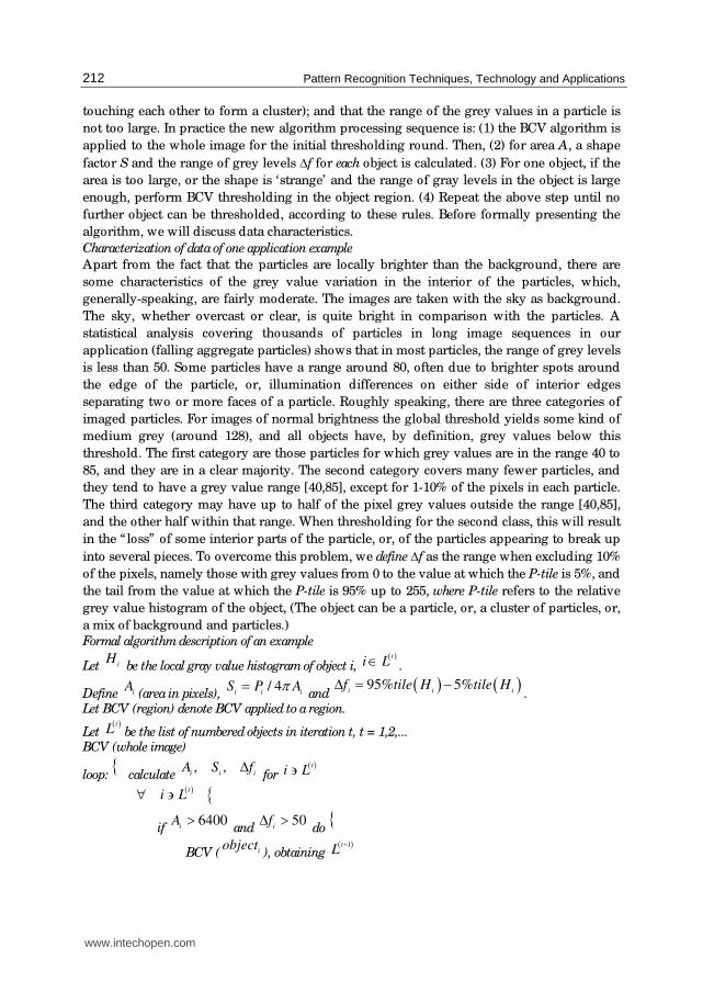
Formal algorithm description of an example

Let iH

be the local gray value histogram of object i, ( )t

i L∈ .

Define iA

(area in pixels), / 4

i i iS P Aπ=

and ( ) ( )95% 5%

i i if tile H tile HΔ = −

. Let BCV (region) denote BCV applied to a region.

Let ( )tL be the list of numbered objects in iteration t, t = 1,2,...

BCV (whole image)

loop: {

calculate , ,

i i iA S fΔ

for ( )t

i L∋

( ) {t

i L∀ ∋

if 6400

iA >

and 50

ifΔ >

do {

BCV ( iobject

), obtaining ( )1tL

+

www.intechopen.com


213

goto loop

}

else

if 1225 6400

iA< <

and 50

ifΔ >

do {

if 2.8

iS >

do {

BCV ( iobject

), obtaining ( )1tL

+

goto loop

}

}

}

}

Fig. 13. Pseudo-code of Algorithm.

When formulating the algorithm below, we let the range test Δf > 50, where 50 is a range

threshold, be a basic criterion determining whether to go on with recursive thresholding in

current objects or not. For large objects consisting of both background and particles, the

range of grey levels need to be large, Δf >50. For touching particles, forming an object

(without background), the range (as defined by Δf) is often, but not always, small. For small

particles (below 35 mm) the range criterion is normally not applicable (bright spots around

the edge of the particle). This is an example of the third category mentioned in the previous

paragraph.

Hence, after global BCV thresholding, each of the objects is labeled and area A and

perimeter P are calculated. Provided the grey value range is sufficiently large (e.g. Δf > 50),

BCV thresholding is applied to an object if it is really large, A > 6400 pixels, or, if it is

sufficiently large, i.e. 1225 < A < 6400 and of ‘complex shape’, where we use a simple shape

factor 2

/ 4S P Aπ= [if more detail shape information is needed, the least squares oriented

Feret box algorithm can be used], defining S > 2.8 as complex shape (from experience, about

hundred images were tested visually and using an interactive program).

Examples

Figure 14 and Table 1 show one example, where Figure 14A illustrates an original image.

After global BCV thresholding, the binarized image is given in Figure 14B. The largest

white object is given a label number 0. Because the object no. 0 has an area greater than

6400 and the range of grey levels is 116, the algorithm does BCV thresholding in the

corresponding area of the original image, and the binarized image is shown in Figure 14C.

In Figure 14C object nos. 1,2, 6, and 9 have an area greater than 1225 pixels. Expect for the

object no. 9, the other three objects had a shape factor 2.8S > , and where selected for

further processing and tests. Out of these three objects, nos. and 2 had a range of gray

levels over 50. At the end of the whole sequence, the algorithm performed BCV

thresholding both for object nos. 1 and 2 in the original image, and the final result is

displayed in Figure 14D. To see if the new algorithm works better than some standard

local / adaptive thresholding techniques, in the next section we will compare two widely-

used thresholding algorithms.

www.intechopen.com


214

particle No. area (square mm) shape factor range of gray level threshold

0, Figure. 5B over 6400 154 - 38 = 116 128

1, Figure. 5C 1804 9.266 122 - 38 = 84 90

2, Figure. 5C 1489 3.442 122 - 49 = 73 93

6, Figure. 5C 1470 3.172 128 - 93 = 35

9, Figure. 5C 2458 2.385 119 - 83 = 36

Table 1. The area, shape and the range of gray levels in the five detected objects.

A B

C D

Fig.14. One example of recursive BCV thresholding performance (see Table 1). A—Original

image. B—After global BCV thresholding. C—After thresholding of object No. 1 in B. D—

Final thresholding result.

www.intechopen.com


215

When the surface of a particle in an image is non-uniform (e.g. three dimensional geometry

property shows up), the particle “ loses” part of its area when the algorithm is applied, as

Figure 15 shown. This is often caused by directional lighting. To avoid this problem, better

to use diffuse lighting.

A B

Fig. 15. An example of recursive BCV thresholding performance on an image. A—After

global BCV thresholding. B—After thresholding of the largest object in A, the arrows

indicate that the two particles “ lost” more than 25% of their area.

3.4 The algorithm for splitting touching particles in a binary image 3.4.1 The algorithm for splitting touching particles It is normal that when a rock particle image is segmented based on its gray level

information, the resulting binary image has often an under-segmentation problem.

Therefore, after image segmentation based on gray-level, an intelligent algorithm is, by

necessity, developed for splitting touching particles in a binary image. The algorithm has

been developed mainly based on shape analysis of rock particles. The split algorithm is a

heuristic search algorithm.

In the past, there were a number of existing algorithms for splitting touching particles, but

not for touching rock particle particles. In general, the existing algorithms first try to find a

pair of cut points on the boundary of a particle (start and end points), and then detect an

optimal cut path or synonymously, split path by using a cost function. To find a pair of cut

points, one may use curvature information around a particle boundary, or ridge information

of a particle, or partial gray level intensity (e.g. strength of local gradient magnitude or

flatness). An optimal path could be detected by using distances, local intensity of gray

levels, or local shape information or combinations thereof.

The existing algorithms cannot be applied for splitting touching rock particles, because the

boundaries of rock particles are rough, the touching parts of rock particles have less local

gray level information, and the touching situations are complex [62]. In the new algorithm for splitting touching rock particles, the main steps are:

www.intechopen.com


216

Polygonal approximation for each object (touching particles): the advantages in this step are

(1) smooth boundary to eliminate concave points caused by boundary roughness; (2) easier

and more accurate calculation of perimeter of a particle, based on detected vertices after

polygonal approximation; (3) in a concave part of an object, only the deepest concave point

in a concave region is detected after polygonal approximation; (4) the degree or classes of

concave points can be determined by both angle and lengths of the intersected lines at a

detecting point; and (5) the opposite direction cone at a concave point is easily and robustly

constructed.

Classification of concavities: the classification of concave points (or concavities) is quite

important for judging if one object is formed by touching particles, and if a hole in an object

should be opened. It is also used for detecting the touching situations, start and end cut points.

Split large clusters into simple clusters: the degrees of touching situations are classified into

(1) two or three touching particles - a simple cluster, (2) multiple touching particles and (3)

multiple touching particles with holes - a large cluster. For the situation (3), the new

algorithm opens holes in some optimal paths, to convert the touching situation (3) to the

touching situation (2) The touching situation (2) then becomes the situation (1) through an

optimal split routine.

Supplementary cost functions for two or three touching particles: when two or three

particles touch and form a cluster, a split path is difficult to correctly search, a simple rule or

criterion easily leads to a wrong split path. The variables such as the shortest distance, the

shortest relative distance, minimum number of unmatched concave points, “opposite

direction” , classes of concavities, area and maximum ratio between two split parts in terms

of areas, are applied for construction of the supplementary cost functions in the new

algorithm.

The algorithm has been tested in an on-line system for measuring crushed rock particles in a

gravitational flow, in which, normally two or three rock particles touching together. In

addition to this, it has also been tested for other different particle images (e.g. crushed rock

particles, natural and rounded rock particles, and potatoes) in which particles touch in a

complicated fashion. The test results show that the algorithm works in a promising way. A

typical example is shown in Fig. 16. In this example, the image binarization is not

satisfactory (Fig. 16(b), but the split result (Fig. 16(c)) is rather good.

(a) (b) (c)

Fig. 16. Example of splitting touching rock particle particles: (a) original image; (b) binarized

image; (c) splitting result.

www.intechopen.com


217

3.4.2 Discussion of the split algorithm The split algorithm consists of three different “treatments” or procedures in a certain order,

namely (1) for holes prevailing inside an object; (2) for multiple touching particles; and (3)

for two or three touching particles. All the three treatments are important for performance

of the whole algorithm. If we do not consider procedures (1) and (2), the split result will be

as shown in Fig. 17(a). Some split paths cross holes or background area.

If one opens holes by using an erosion procedure instead (say, repeating three times), then

uses procedure (2) and (3) to split particles, the split result (Fig. 17(b)) is better than that of

Fig. 17(a). However, in Fig. 17(b), some particles result from split, including new concave

parts, and some touching particles are still not split completely or over-split. This takes place

because erosion with a fixed number of iterations is not flexible enough. Note that parallel

dilation after erosion cannot preserve the shape of particle.

(a) (b)

Fig. 17. Two split results on the image in Fig. 19 (a): (a) split result without hole opening and

without the procedure for multiple touching particles; (b) split result after opening holes by

erosion of objects three times followed by split and parallel dilation, of objects.

In the algorithm, one principal part is procedure (3), based on polygonal approximation.

Without polygonal approximation, the classification and the detection of concave points are

difficult to carry out. As described before, in most previous algorithms, a concave point is

detected by the use of an angle or a curvature threshold. The angle is constructed by two

chord lines with equally number of pixels, are usually determined by experience.. The

following figures show an angle calculated by using two chord lines, each of them crossed 4

pixels (Fig. 18(a)); and an angle calculated by using two chord lines, each of them crossed 8-

19 pixels (Fig. 18(b)), where the number of pixels on a chord line increases as the perimeter

of the object increases. In both cases, the threshold for detecting a significant concave point

is 64 degrees (angle 0

64α ≤ ). The images in Fig. 18 (white points are detected significant

concave points) show that short chord lines give a rather precise detection of concave points,

but, however, many scattered irrelevant candidates for the cut points (start and end points)

www.intechopen.com


218

are obtained (Fig. 18(a)). On the other hand, long chord lines are good in signalling

significant concave part (Fig. 18(b)), but there are too many adjacent candidates of cut points

(fragmented and non-fragmented) located closely to the true significant concave point. In

these cases, one has to develop special procedures to search for start and end points for

candidates of split paths.

(a) (b)

Fig. 18. Significant concave points detected by using two chord lines, each of them crossed

the same number of pixels (angle 0

64α ≤ ): (a) each of the two chord lines crosses 4 pixels;

(b) each of the two chord lines crosses a q pixel, where [ ]8,19q∈ depending on object size

(e.g. area or perimeter).

Figure 18 illustrates that the angle obtained in reference, so-called k-curvature, is quite

sensitive to choice of lengths of 2-vertex lines (chords).

3.4.3 Test results of the algorithm The new split algorithm has been tested for aggregate images from muckpiles, laboratories,

conveyor belts and gravity flows. The test results show that it works in a promising way.

In a quarry of central Sweden (Västerås), an on-line system for the analysis of size and shape

of aggregates in a gravitational flow, i.e. falling particles, was set-up. An interlaced CCD

camera acquires aggregate images from a gravity flow at a speed of 25 frames per second.

The odd-lines images were transferred into a PC computer with a resolution 256x256x8 bits.

The system first checks the image quality (if the image is qualified for further processing or

not, e.g. blurry or empty images cannot be chosen for further processing). When an image

passes this checkpoint, image binarisation is performed. After this, investigating 1000

particles in 52 binary images, on average, there are 40% particles with a touching problem,

and normally two or three particles touch together, and just a few clusters consist of 5-6

particles without holes. In order to resolve this kind of touching problem, a procedure of the

split algorithm described in this article, for splitting two or three touching particles, is

applied to all the binarised images, and finally size and shape of aggregates are analysed.

www.intechopen.com


219

The system has been tested for about two months. It takes about ten minutes to process

twenty images as one analysis data set, yielding size or shape distributions. Traditional

sieving analysis results show that there is 5-10% of aggregate for which the size is over 64

mm. Performed image analysis also yields the same results, which indicates that either there

are no touching problems or the new split algorithm works.

In order to clarify the issue, two hundred images were randomly picked up from all data.

Out of all the images, only 21 of them had no touching problem. The number of clusters in

the other 179 images was about 1602. A comparison between before and after splitting has

been carried out by human vision; 90% of the clusters have been completely split by using

the new splitting procedure for two or three touching particles. In the other 10% of clusters,

4% are over-split due to concavity errors caused by noise, and 6% are under-split due to

omission of some existing concavities not very significant for the algorithm. These two

opposite situations may be related to concavity classification in the algorithm. The detail

results are listed in Table 2. Split results from two example images are shown in Figs. 19-20.

No. of images No. of

particles No. of clusters

Over-split

clusters

Under-split

clusters Fully split clusters

200 3815 1602 63 91 1448

Table 2. Test results in an on-line system

(a) (b) (c)

Fig. 19. Example #1 of split result of aggregate images from a gravitational flow: (a) original

image; (b) binary image; (c) split result, used thresholds: 0 0

1 2 3 1 2( , , , , ) (6,0.5,0.6,100 ,60 )L L L α α = .

We have tested the algorithm on a number of rock particle images with different situations

of touching particles. The following examples illustrate the power of the split algorithm on

realistic data for images of packed particles. The following figures show examples of split

results from our split algorithm consisting of three main procedures: filling and opening

holes, splitting multiply touching particles, and splitting two or three touching particles,

which has been applied in an on-line system. Different grey shades in binary images are for

different clusters (one object = one cluster) before split.

In Fig. 21(a), the image is a binarised image, and the original image is taken from a laboratory, of crushed aggregate particles of different sizes. The image includes two large clusters and one single particle, and the split result image (Fig. 21(c)) shows that two large

clusters were completely split into 54 particles.

www.intechopen.com


220

In Fig. 22(a), an original aggregate (natural) image is presented, taken from a conveyor belt

in the laboratory. Although manual binarisation result (Fig. 22(b)) is not very satisfactory,

the split result is quite promising.

(a) (b) (c)

Fig. 20. Example #2 of split result of aggregate images from a gravitational flow: (a) original

image; (b) binary image; (c) split result, used thresholds: 0 0

1 2 3 1 2( , , , , ) (6,0.5,0.6,100 ,60 )L L L α α = .

(a) (b) (c)

Fig. 21. Split result of touching particles of crushed aggregates: (a) a binary image taken with

the illumination of backlighting, consisting of two clusters and one single particle; (b) the

image after hole treatment; (c) the image after split, consisting of 55 particles.

The new algorithm for splitting touching rock particles is developed based on polygonal

approximation. It includes classification of concavities and analysis of supplementary cost

functions. The whole procedure consists of three major steps: (1) two or three touching

particles; (2) multiple touching particles; and (3) holes prevailing inside an object. The

algorithm can be applicable not only to crushed rock particle images, but also to other

particle images, e.g. cells or chromosomes, or cytological, histological, metallurgical or

agricultural images.

www.intechopen.com


221

(a) (b) (c)

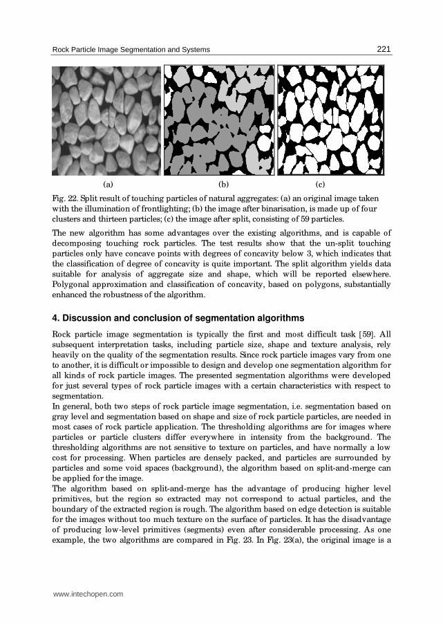
Fig. 22. Split result of touching particles of natural aggregates: (a) an original image taken

with the illumination of frontlighting; (b) the image after binarisation, is made up of four

clusters and thirteen particles; (c) the image after split, consisting of 59 particles.

The new algorithm has some advantages over the existing algorithms, and is capable of

decomposing touching rock particles. The test results show that the un-split touching

particles only have concave points with degrees of concavity below 3, which indicates that

the classification of degree of concavity is quite important. The split algorithm yields data

suitable for analysis of aggregate size and shape, which will be reported elsewhere.

Polygonal approximation and classification of concavity, based on polygons, substantially

enhanced the robustness of the algorithm.

4. Discussion and conclusion of segmentation algorithms

Rock particle image segmentation is typically the first and most difficult task [59]. All

subsequent interpretation tasks, including particle size, shape and texture analysis, rely

heavily on the quality of the segmentation results. Since rock particle images vary from one

to another, it is difficult or impossible to design and develop one segmentation algorithm for

all kinds of rock particle images. The presented segmentation algorithms were developed

for just several types of rock particle images with a certain characteristics with respect to

segmentation.

In general, both two steps of rock particle image segmentation, i.e. segmentation based on

gray level and segmentation based on shape and size of rock particle particles, are needed in

most cases of rock particle application. The thresholding algorithms are for images where

particles or particle clusters differ everywhere in intensity from the background. The

thresholding algorithms are not sensitive to texture on particles, and have normally a low

cost for processing. When particles are densely packed, and particles are surrounded by

particles and some void spaces (background), the algorithm based on split-and-merge can

be applied for the image.

The algorithm based on split-and-merge has the advantage of producing higher level

primitives, but the region so extracted may not correspond to actual particles, and the

boundary of the extracted region is rough. The algorithm based on edge detection is suitable

for the images without too much texture on the surface of particles. It has the disadvantage

of producing low-level primitives (segments) even after considerable processing. As one

example, the two algorithms are compared in Fig. 23. In Fig. 23(a), the original image is a

www.intechopen.com


222

fragments image taken from a rockpile. Where, fragments show multiple faces in the image,

and natural light caused illumination non-uniform. The two algorithms were used for

segmenting the original image without any preprocessing. The image in Fig. 23(c) is a

thresholded edge image without doing noise edge deleting and gap linking. The algorithm

based on edge detection is very sensitive to this kind of image. The algorithm based on split-

and-merge can not exactly extract every individual fragment.

(a) (b) (c)

Fig. 23. Comparison between two segmentation algorithms. (a) Original fragment image

from a rockpile. (b) Image segmented by the algorithm based on split-and-merge. (c) Edge

image processed by Canny’s edge detector.

The algorithm for splitting touching particles in a binary image is important for overcoming

the problem of over-segmentation in a gray level image. In most cases, as discussed before,

any single one of the gray level segmentation algorithms cannot segment a gray level image

completely. As a supplementary procedure, the segmentation algorithms based on rock

particle shapes should be used for further segmentation.

In conclusions, segmentation algorithm selection is based on the types of rock particle

images and requirement of measuring rock particles. If one needs a crude segmentation

result for densely packed rock particle image, the algorithm based on edge detection will be

very useful. The algorithm based on thresholding often lead to an under-segmentation

problem, which can be resolved by using the split algorithm for touching particles. The

algorithm based on split-and-merge is a combination of segmentation on gray level and

segmentation based on shape of rock particles. The algorithm includes several techniques

such as image pre-processing, region split-and-merge, thresholding, binary image

segmentation. Combinations of the mentioned segmentation algorithms are more powerful

than the individual procedures by themselves.

5. References

Wang, W.X. and Fernlund, J., Shape Analysis of Rock particles. KTH-BALLAST Report no.

2, KTH, Stockholm, Sweden (1994).

Gallagher, E., Optoelectronic coarse particle size analysis for industrial measurement and

control. Ph.D. thesis, University of Queensland, Dept. of Mining and Metallurgical

Engineering (1976).

www.intechopen.com


223

Nyberg, L., Carlsson, O., Schmidtbauer, B., Estimation of the size distribution of fragmented

rock in ore mining through automatic image processing. Proc. IMEKO 9th World

Congress, May, Vol. V/ III (1982), pp. 293 - 301.

Hunter, G.C., et al., A review of image analysis techniques for measuring blast

fragmentation. Mining Science and Technology, 11 (1990) 19-36.

Franklin, J.A, Kemeny J.M. and Girdner, K.K., Evolution of measuring systems: A review.

Measurement of Blast Fragmentation, Ed by J.A. Franklin and T. Katsabanis,

Rotterdam: Balkema (1996), 47-52.

Wang, W.X. and Dahlhielm, S., Evaluation of image methods for the size distribution of

rock fragments after blasting. Report no. 1 on the project within the Swedish-Sino

cooperation in metallic materials and mining, Luleå, Sweden, October (1989).

Lange, T., Real-time measurement of the size distribution of rocks on a conveyor belt. Int.

Fed. Automatic control, Workshop on applied Measurements in Mineral and Metal

Processing, Johannesburg (1989).

Lang, T.B., Measurement of the size distribution of rock on a conveyor belt using machine

vision. Ph.D. thesis, the Faculty of Engineering, University of the Witwatersrand,

Johannesburg (1990).

Zeng, S., Wang, Y. and Wang, W.X., Study on the techniques of photo -image analysis for

rock fragmentation by blasting. Proc. for third period of Sino-Swedish joint

research on science and technology of metallurgy, Publishing House of

Metallurgical Industry, China (1992), pp. 103-115.

Wang, Y., Zeng, S. and Wang, W.X., Study on the image analysis system of photographic

film. Proc. for third period of Sino-Swedish joint research on science and

technology of metallurgy, Publishing House of Metallurgical Industry, China

(1992), pp. 116-126.

Montoro, J..J. and Gonzalez, E., New analytical techniques to evaluate fragmentation based

on image analysis by computer methods. 4th Int. Symp. Rock Fragmentation by

Blasting, Keystone, Vienna, Austria (1993), pp. 309 -316.

McDermott, C., Hunter, G.C. and Miles, N.J., The application of image analysis to the

measurement of blast fragmentation. Symp. Surface Mining-Future Concepts,

Nottingham University, Marylebone Press, Manchester (1989), pp. 103-108.

Ord, A., Real time image analysis of size and shape distributions of rock fragments. Proc.

Aust. Int. Min. Metall., 294, 1 (1989).

Lin, C.L and Miller, J.D., The Development of a PC Image-Based On-line Particle Size

Analyzer. Minerals & Metallurgical Processing, No. 2 (1993) 29-35.

Von Hodenberg, M., Monitoring crusher gap adjustment using an automatic particle size

analyzer, Mineral process, Vol. 37, (1996) 432-437 (Germany).

HAVER CPA, Computerized particle analyzer, User’s Guide :CPA - 3, Printed by HAVER &

BOECKER, Drahtweberei, Ennigerloher Straβe 64, D-59302 OELDE Westfalen,

(1996).

Blot, G. and Nissoux, J.-L., Les nouveaux outils de controle de la granulométrie et de la

forme (New tools for controlling size and shape of rock particles), Mines et

carrières, Les Techniques V/ 94, SUPPL.-Déc., Vol. 96, (1994) (France).

J. Schleifer and B. Tessier, Fragmentation Assessment using the FragScan System: Quality of

a Blast, Fragblast, Volume 6, Numbers 3-4 / December 2002, pp. 321 - 331,

Publisher: Taylor & Francis.

www.intechopen.com


224

Grannes, S.G., Determine size distribution of moving pellets by computer image processing,

19th Application of Computers and Operations Reaserch in Mineral

Industry(editor, R.V. Ramani), Soc. Mining Engineers, Inc. (1986), pp. 545-551.

Donald, C. and Kettunen, B.E., On-line size analysis for the measurement of blast

fragmentation. Measurement of Blast Fragmentation , Ed by J.A. Franklin and T.

Katsabanis. Rotterdam: Balkema, (1996) 175-177.

Norbert H Maerz, Tom W, Palangio. Post-Muckpile, Pre-Primary Crusher, Automated

Optical Blast Fragmentation Sizing, Fragblast, Volume 8, Number 2 / June 2004,

pp. 119 – 136, Publisher: Taylor & Francis.

Norbert H. Maerz and Wei Zhou , Calibration of optical digital fragmentation measuring

systems, Fragblast, Volume 4, Number 2 / June 2000, pp. 126 - 138, Publisher:

Taylor & Francis..

Paley, N., Lyman, G..J. and Kavetsky, A., Optical blast fragmentation assessment, Proc. 3rd

Int. Symp. Rock Fragmentation by Blasting, Australian IMM, Brisbane, Australia

(1990), pp. 291-301.

Wu, X., and Kemeny, J.M., A segmentation method for multiconnected particle delineation,

Proc. of the IEEE Workshop on Applications of Computer vision, IEEE Computer

Society Press, Los Alamitos, CA (1992) 240-247.

Kemeny J, Mofya E, Kaunda R, Lever P. Improvements in Blast Fragmentation Models

Using Digital Image Processing, Fragblast, Volume 6, Numbers 3-4 / December

2002, pp. 311 - 320, Publisher: Taylor & Francis.

.Kemeny, J., A practical technique for determining the size distribution of blasted benches,

waste dumps, and heap-leach sites, Mining Engineering, Vol. 46, No. 11 (1994),

1281-1284.

Girdner, K.K., Kemeny, J..M., Srikant, A. and McGill, R., The split system for analyzing the

size distribution of fragmented rock. Measurement of Blast Fragmentation, Ed by

J.A. Franklin & T. Katsabanis. Rotterdam: Balkema (1996), pp. 101-108.

Vogt, W. and Aβbrock, Digital image processing as an instrument to evaluate rock

fragmentation by blasting in open pit mines, 4th Int. Symp. Rock fragmentation by

Blasting, Keystone, Vienna, Austria (1993), 317-324.

Havermann, T. and Vogt, W., TUCIPS. A system for the estimation of fragmentation after

production blasts, Measurement of Blast Fragmentation, Ed by J.A. Franklin and T.

Katsabanis. Rotterdam: Balkema (1996), pp. 67-71.

Rholl, S.A., et al., Photographic assessment of the fragmentation distribution of rock quarry

muckpiles, 4th Int. Symp. Rock Fragmentation by Blasting, Vienna, Austria (1993),

pp. 501-506.

Lin, C.L, Yen, Y.K. and Miller, J.D. , On-line coarse particle size measurement -industrial

testing. SME Annual Meeting, March 6-9, Denver, Colorado, USA, (1995).

Bedair A., Daneshmend L.K. and Hendricks C.F.B. Comparative performance of a novel

automated technique for identification of muck pile fragment boundaries.

Measurement of Blast Fragmentation, Ed by J.A. Franklin & T. Katsabanis.

Rotterdam: Balkema, (1996) 157-166.

Bedair, A., Digital image analysis of rock fragmentation from blasting. Ph.D. thesis,

Department of Mining and Metallurgical Engineering, McGill University, Montreal,

Quebec (1996).

www.intechopen.com


225

Wang, W.X. and Dahlhielm, S., An algorithm for automatic recognition of rock

fragmentation through digitizing photo images, Report no. 5 on the project within

the Swedish-Sino cooperation in metallic materials and mining, July (1990).

Stephansson, O., Wang, W.X. and Dahlhielm, S., Automatic image processing of rock

particles, ISRM Symposium: EUROCK '92, Chester, UK, 14-17 September, British

Geotechnical Society, London, UK (1992), pp. 31-35.

Wang, W. X., Automatic Image Analysis of Rock particles from A Moving Conveyor Belt.

Licentiate Thesis. Dept. of Civil and Environmental Engineering, Royal Institute of

Technology, Stockholm, Sweden (1995).

Dahlhielm, S., Industrial applications of image analysis. The IPACS system. Measurement of

Blast Fragmentation, Ed by J.A. Franklin & T. Katsabanis. Rotterdam: Balkema

(1996), pp. 59-65.

Yen, Y. K., Lin, C. L. and Miller, J. D., The overlap problem in on-line coarse size

measurement - segmentation and transformation, SME Annual Meeting, February

14-17, Albuquerque, New Mexico, US. (1994), Preprint No. 94-177.

Schleifer, J. and Tessier, B., FRAGSCAN: A tool to measure fragmentation of blasted rock.

Measurement of Blast Fragmentation, Ed by J.A. Franklin and T. Katsabanis.

Rotterdam: Balkema (1996), pp. 73-78.

Cheimanoff, N.M., Chavez, R. and Schleifer, J., FRAGMENTATION: A scanning tool for

fragmentation after blasting, 4th Int. Symp. Rock Fragmentation by Blasting,

Keystone, Vienna, Austria (1993), pp. 325-330.

Chung S.H., Experience in fragmentation control. Measurement of Blast Fragmentation, Ed

by J.A. Franklin & T. Katsabanis. Rotterdam: Balkema (1996), pp. 247-252.

LIN, C.L., Miller, J.D., Luttrell, G.H. and Adel, G.T., On-line washability analysis for the

control of coarse coal cleaning circuits, SME/ AIME, Editor S.K. Kawatra

(1995), pp. 369-378.

Fua, P. and Leclerc, Y.G., Object-centered surface reconstruction: Combining multi-image

stereo and shading. International Journal of Computer Vision, Vo. 16, No. 1 (1995),

35-56.

Parkin, R.M., Calkin, D.W. and Jackson, M.R., Roadstone rock particle: An intelligent opto-

mechatronic product classifier for sizing and grading. Mechanics Vol. 5, No. 5,

Printed in Great Britain (1995), 461-467.

Cheung, C.C. and Ord, A., An on line fragment size analyzer using image processing

techniques, 3rd Int. Symp. Rock Fragmentation by Blasting, Brisbane, August 26 -31

(1990), pp. 233-238.

Liang, J., Intelligent splitting the chromosome domain, Pattern Recognition, Vol. 22, No. 5

(1989), pp. 519-532.

Yeo, X.C., Jin, S.H., Ong, Jayasooriah and R. Sinniah, Clump splitting through concavity

analysis, Pattern Recognition Lett. 15, (1994), pp. 1013-1018.

Otsu, N., A threshold selection method from gray-level histogram, IEEE Trans. Systems

Man Cybernet, SMC-9 (1979), pp. 62-66.

Tor, N., Sven, H., Wang, W.X. and Dahlhielm, S., System för bildtolking av

kornstorleksfördelning i naturmaterial och förädlat material, BDa-raport 1, March

(1991), (for vägverket in Luleå).

www.intechopen.com


226

Tor, N., Sven, H., Wang, W.X. and Dahlhielm, S., System för bildtolking av

kornstorleksfördelning i naturmaterial och förädlat material, BDa-raport 2, October

(1991), (for vägverket in both Borlänge and Luleå).

Jansson, M. and Muhr, T., A study of geometric form of ballast material (in Swedish). Ms.

thesis. Dept. of Civil and Environmental Engineering, Royal Institute of

Technology, Stockholm, Sweden, EX-1995-002 (1995).

Wang, W.X., 2006, Image analysis of particles by modified Ferret method – best-fit rectangle,

International Journal: Powder Technology, Vol. 165, Issue 1, pp. 1-10.

Wang, W.X., 2008, Fragment Size Estimation without Image Segmentation, International

Journal: Imaging Science Journal, Vol. 56, p.91-96, April, 2008

Wang, W.X. and Bergholm, F., On edge density for automatic size inspection, Theory and

Applications of Image Analysis II, Ed by Gunilla Borgefors, publisher World

Scientific Publishing Co. Pte. Ltd. Singapore (1995), pp. 393-406.

Weixing Wang, 2007, An Image Classification and Segmentation for Densely Packed

Aggregates, LNAI, Vol. 4426, pp.887-894.

Norbert, H. M., Image sampling techniques and requirements for automated image analysis

of rock fragmentation. Measurement of Blast Fragmentation, Ed by J.A. Franklin

and T. Katsabanis. Rotterdam: Balkema (1996), pp. 47-52.

Michael, W. B., Image Acquisition, (handbook of machine vision engineering volume I ),

Printed in Great Britain at The Alden Press, Oxford. ISBN 0 412 47920 6., Published

by Chapman & Hall, 2-6 Boundary Row, London SE1 8HN, UK., (1996), pp. 1, 109-

126, 127-136, 169, 229-239.

Bir, B. and Sungkee, L., Genetic Learning for Adaptive Image Segmentation, Kluwer

Academic Publishers, USA.(1994), pp. 2-4.

Cany, J.F., A computational approach to edge detection, IEEE Trans. Pattern Analysis.

March. Intell. 8 (1986), pp. 679-698.

Suk, M., and Chung, S.M., A new image segmentation technique based on partition mode

test. Pattern Recognition Vol. 16, No. 5. (1983), pp. 469-480.

Wang, W.X., 1998, Binary image segmentation of aggregates based on polygonal

approximation and classification of concavities. International Journal: Pattern

Recognition, 31(10), 1503-1524..

Wang, W.X., 1999, Image analysis of aggregates, International Journal: Computers &

Geosciences 25, 71-81..

Jansson, M. and Muhr, T., Field tests of an image analysis system for ballast on a conveyor

belt in three quarries in Sweden (in Swedish). Technical Report. KTH-Ballast,

Stockholm, Sweden. ISNN 1400-1306 (1995).

Cunningham, C.V.B., Fragmentation estimates and the Kuz-Ram model four years on. 2nd

Int. Symp. on Rock Fragmentation by Blasting, Keystone, USA (1987), pp. 475-487.

www.intechopen.com

Pattern Recognition Techniques, Technology and ApplicationsEdited by Peng-Yeng Yin

ISBN 978-953-7619-24-4Hard cover, 626 pagesPublisher InTechPublished online 01, November, 2008Published in print edition November, 2008

InTech EuropeUniversity Campus STeP Ri Slavka Krautzeka 83/A 51000 Rijeka, Croatia Phone: +385 (51) 770 447 Fax: +385 (51) 686 166www.intechopen.com

InTech ChinaUnit 405, Office Block, Hotel Equatorial Shanghai No.65, Yan An Road (West), Shanghai, 200040, China

Phone: +86-21-62489820 Fax: +86-21-62489821

A wealth of advanced pattern recognition algorithms are emerging from the interdiscipline betweentechnologies of effective visual features and the human-brain cognition process. Effective visual features aremade possible through the rapid developments in appropriate sensor equipments, novel filter designs, andviable information processing architectures. While the understanding of human-brain cognition processbroadens the way in which the computer can perform pattern recognition tasks. The present book is intendedto collect representative researches around the globe focusing on low-level vision, filter design, features andimage descriptors, data mining and analysis, and biologically inspired algorithms. The 27 chapters coved inthis book disclose recent advances and new ideas in promoting the techniques, technology and applications ofpattern recognition.

How to referenceIn order to correctly reference this scholarly work, feel free to copy and paste the following:

Weixing Wang (2008). Rock Particle Image Segmentation and Systems, Pattern Recognition Techniques,Technology and Applications, Peng-Yeng Yin (Ed.), ISBN: 978-953-7619-24-4, InTech, Available from:http://www.intechopen.com/books/pattern_recognition_techniques_technology_and_applications/rock_particle_image_segmentation_and_systems

© 2008 The Author(s). Licensee IntechOpen. This chapter is distributedunder the terms of the Creative Commons Attribution-NonCommercial-ShareAlike-3.0 License, which permits use, distribution and reproduction fornon-commercial purposes, provided the original is properly cited andderivative works building on this content are distributed under the samelicense.

https://creativecommons.org/licenses/by-nc-sa/3.0/

rock particle image segmentation and systemscdn.intechweb.org/pdfs/5786.pdf · rock particle image...

Documents