geosciences

Article

Rock Mass Characterization of Karstified Marbles andEvaluation of Rockfall Potential Based on Traditionaland SfM-Based Methods; Case Study of Nestos, Greece

George Papathanassiou 1,* , Adrián Riquelme 2 , Theofilos Tzevelekis 1

and Evaggelos Evaggelou 1

1 Department of Civil Engineering, Democritus University of Thrace, 67100 Xanthi, Greece;thtzebel@civil.duth.gr (T.T.); eevange@civil.duth.gr (E.E.)

2 Department of Civil Engineering, University of Alicante, 03690 Alicante, Spain; ariquelme@ua.es* Correspondence: gpapatha@civil.duth.gr

Received: 1 September 2020; Accepted: 25 September 2020; Published: 28 September 2020 �����������������

Abstract: Rockfall consists one of the most harmful geological phenomena for the man-madeenvironment. In order to evaluate the rockfall hazard, a variety of engineering geological studiesshould be realized, starting from conducting a detailed field survey and ending with simulatingthe trajectory of likely to fail blocks in order to evaluate the kinetic energy and the runout distance.The last decade, new technologies, i.e., remotely piloted aircraft systems (RPAS) and light detectionand ranging (LiDAR) are frequently used in order to obtain and analyze the characteristics of therock mass based on a semi-automatic or manual approach. Aiming to evaluate the rockfall hazard inthe area of Nestos, Greece, we applied both traditional and structure from motion (SfM)-orientedapproaches and compared the results. As an outcome, it was shown that the semi-automatedapproaches can accurately detect the discontinuities and define their orientation, and thus can beused in inaccessible areas. Considering the rockfall risk, it was shown that the railway line in thestudy area is threaten by a rockfall and consequently the construction of a rockfall netting mesh or arock shed is recommended.

Keywords: RPAS; rockfall; classification; potential, SMR; trajectory; marbles

1. Introduction

The methodology that is usually followed for the evaluation of rockfall potential within an area isdiscriminated in several stages, including a detailed engineering geology field survey and analysisof the data obtained during this survey, identification of the failure type mechanism, e.g., wedge,planar slide, toppling, and the assessment of the rockfall trajectory and the evaluation of criticalparameters like the kinetic energy and the bounce height of the detached rock (e.g., [1]).

The first phase of this methodology focusses on the in situ characterization of the rock mass whichis based on the information provided by the field survey. Specific parameters, such as the structure of therock mass and the quality of the discontinuities, the joint spacing, the filling material, etc., are quantifiedand described to assess the rock mass quality. The most applied rock mass classification systems are therock mass rating (RMR) [2], the Q-system [3] and the geological strength index (GSI) [4,5]. The first twoapproaches provide a semi-quantitative value of their rock mass quality through an index, while theclassification based on the GSI system results to a number which, when combined with the intactrock properties, can be used for estimating the reduction in rock mass strength for different geologicalconditions [6]. Having classified the rock mass and defined critical parameters of its structure, i.e.,identification of the discontinuity sets and their orientation, a rockfall hazard analysis can follow.

Geosciences 2020, 10, 389; doi:10.3390/geosciences10100389 www.mdpi.com/journal/geosciences

Geosciences 2020, 10, 389 2 of 20

A rockfall is a fragment of rock detached by sliding, toppling, or falling that falls along a verticalor sub-vertical cliff, proceeds down slope by bouncing and flying along ballistic trajectories or byrolling on talus or debris slopes [7]. Although the fact that rockfall usually impacts only small areas,the damage to the infrastructure or persons directly affected may be high with serious consequences [8].Rockfalls range from small cobles to large boulders hundreds of cubic meters in size and travel atspeeds ranging from few to tens of meters per second [9]. Minor rockfalls affect most of the rockslopes, whereas large size ones such as cliff falls and rock avalanches, affect only great rock slopes withgeological conditions favorable to instability [10].

The main factors that can trigger the detachment of a rock from a slope are rainfall, earthquakes,and human activities while the fall of a rock is determined by factors like the slope morphology [11].In addition, the joint roughness number, the joint alteration number, and the joint water reduction areimportant variables. The generation of rockfall is a rapid phenomenon and represents a continuoushazard in mountain areas worldwide. Rockfall presents an ongoing challenge to the safe operationof transportation infrastructure, creating hazardous conditions which can result in damage to roadsand railways [12–15], as well as loss of life [16]. As it has been demonstrated by [17], relatively smallvolumes of rocks may cause significant damage and traffic disruption, particularly in railroads.

In order to evaluate the rockfall hazard in an area and/or document the effects of a case study, remotesensing techniques were developed during the last decades such as light detection and ranging (LiDAR)(e.g., [18,19]) and photogrammetric surveys. The latter one, a photogrammetric survey, is frequentlyconducted using remotely piloted aircraft systems (RPAS), as well known as unmanned aerial vehicles(UAV), such as multicopters equipped with webcams, digital cameras and other sensors [20–24], for diverseapplications such as 3D terrain analysis, slope stability, mass movement hazard, and risk management [25].RPASs provide an easy to use and low-cost remote sensing platform for rockfall studies, considered thathigh-resolution imagery can be acquired in short time in inaccessible areas. Using the structure frommotion (SfM) image processing technique, a 3D point cloud can be created by intersecting the matchedfeatures between the overlapping, offset images [26].

The developed 3D point cloud can be proceeded for conducting a semi-automated or manuallystructural analysis, and for extracting information regarding the discontinuity sets, i.e., orientation andjoint spacing [27–32]. Having obtained these data, the evaluation of rockfall potential can be realizedby performing a kinematic analysis (e.g., [33–36]). In addition, the combination of this approach withtraditional engineering geological field surveys results to a rock mass classification and to slope massrating assessment [37,38].

This study focuses on the area of Nestos, Greece, at a site where the national railway, connectingGreece and Turkey, passes in a short distance (<10 m) from a vertical cliff of marble. The marble unitis the dominant formation in the research area, consisted by massive white marbles with dolomitelayers. These marbles appear to be karstic on the surface in many places. The rock slope studied forthe purposes of this research is a white to light grey colored poorly bedded massive marbles of 35 mhigh (Figure 1).

Geosciences 2020, 10, 389 3 of 20Geosciences 2020, 10, x FOR PEER REVIEW 3 of 19

Figure 1. (a) Black circle indicates the location of the study area at Northeastern Greece; (b) simplified geological map (1:50,000 scale) of the wider area modified by [39], where the study area is defined with a black square; (c) red square indicates the location of the study area on aerial imagery (image source: © Google Earth; Digital Globe 2020); (d) perspective view of the slope, (e) generated 3D point cloud of site 2, (f) and generated 3D point view of site 1.

Figure 1. (a) Black circle indicates the location of the study area at Northeastern Greece; (b) simplifiedgeological map (1:50,000 scale) of the wider area modified by [39], where the study area is defined witha black square; (c) red square indicates the location of the study area on aerial imagery (image source:© Google Earth; Digital Globe 2020); (d) perspective view of the slope, (e) generated 3D point cloud ofsite 2, (f) and generated 3D point view of site 1.

The goal of this study is twofold: (i) to perform a rock mass classification in order to evaluatethe rockfall potential by assigning slope mass rating (SMR) index values, and (ii) to simulate thetrajectories of likely to fail blocks in order to examine their run-out distance and to assess the rockfallhazard on the railway line. In order to achieve this goal, a RPAS survey conducted, and a 3D pointcloud was generated (Figure 1). The lower part of the rock slope, i.e., site 1 was investigated both bytraditional field survey and point-cloud approaches while the higher part (site 2) was analyzed basedon the generated 3D model. The procedure that was followed in this study is shown in the followingflowchart (Figure 2).

Geosciences 2020, 10, 389 4 of 20

Geosciences 2020, 10, x FOR PEER REVIEW 4 of 19

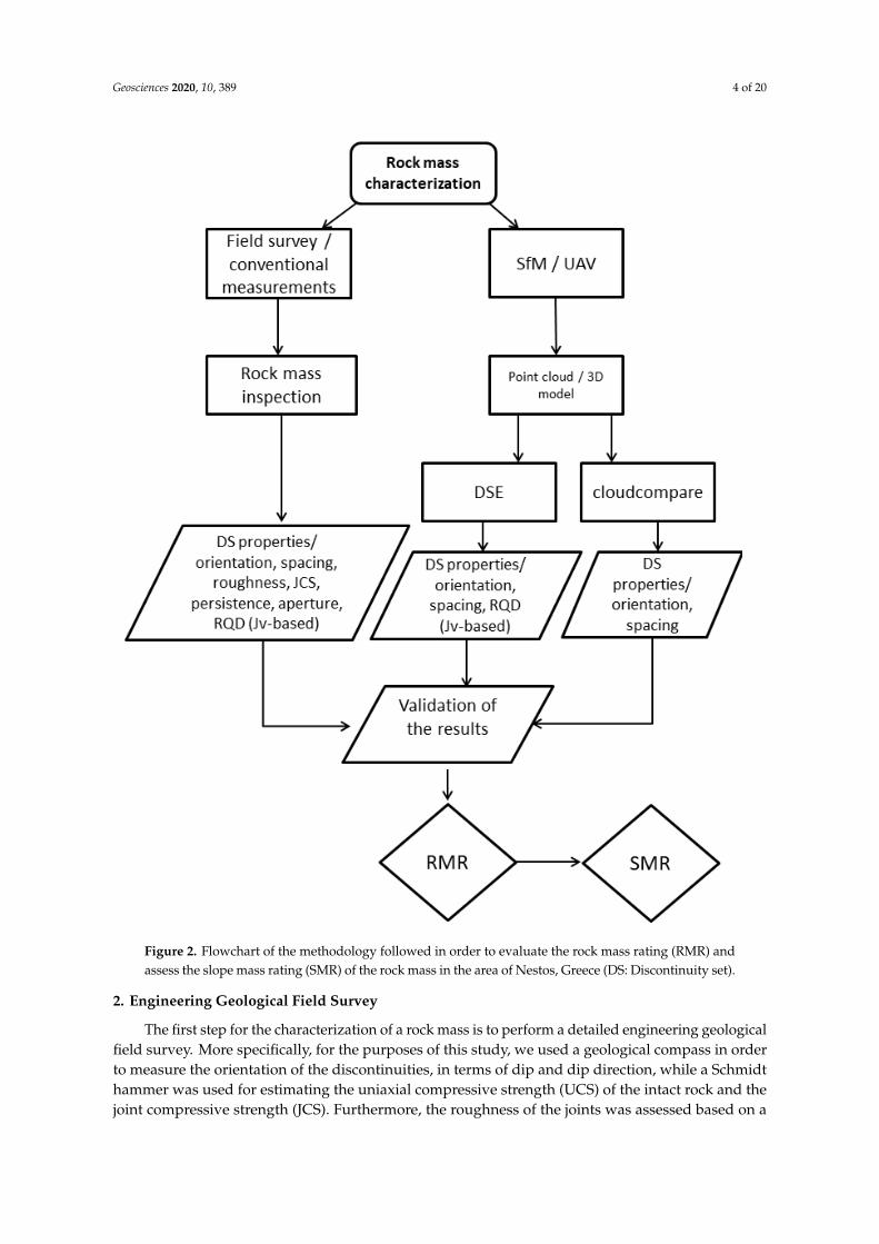
Figure 2. Flowchart of the methodology followed in order to evaluate the rock mass rating (RMR) and assess the slope mass rating (SMR) of the rock mass in the area of Nestos, Greece (DS: Discontinuity set).

2. Engineering Geological Field Survey

The first step for the characterization of a rock mass is to perform a detailed engineering geological field survey. More specifically, for the purposes of this study, we used a geological compass in order to measure the orientation of the discontinuities, in terms of dip and dip direction, while a Schmidt hammer was used for estimating the uniaxial compressive strength (UCS) of the intact rock and the joint compressive strength (JCS). Furthermore, the roughness of the joints was assessed based on a profilometer while the aperture and joint spacing were measured using a

Figure 2. Flowchart of the methodology followed in order to evaluate the rock mass rating (RMR) andassess the slope mass rating (SMR) of the rock mass in the area of Nestos, Greece (DS: Discontinuity set).

2. Engineering Geological Field Survey

The first step for the characterization of a rock mass is to perform a detailed engineering geologicalfield survey. More specifically, for the purposes of this study, we used a geological compass in orderto measure the orientation of the discontinuities, in terms of dip and dip direction, while a Schmidthammer was used for estimating the uniaxial compressive strength (UCS) of the intact rock and thejoint compressive strength (JCS). Furthermore, the roughness of the joints was assessed based on a

Geosciences 2020, 10, 389 5 of 20

profilometer while the aperture and joint spacing were measured using a surveyor’s tape. Finally,the filling material and the weathering conditions at the area were also assessed.

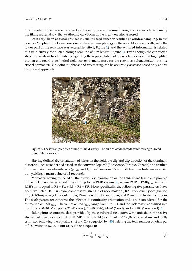
Data acquisition of discontinuities is usually based either on scanline or window sampling. In ourcase, we “applied” the former one due to the steep morphology of the area. More specifically, only thelower part of the rock face was accessible (site 1, Figure 1), and the acquired information is relatedto a field survey conducted along a scanline of 4 m length (Figure 3). Even though the conductedstructural analysis has limitations regarding the representation of the whole rock face, it is highlightedthat an engineering geological field survey is mandatory for the rock mass characterization sincecrucial parameters, e.g., joint roughness and weathering, can be accurately assessed based only on thistraditional approach.

Geosciences 2020, 10, x FOR PEER REVIEW 5 of 19

surveyor’s tape. Finally, the filling material and the weathering conditions at the area were also assessed.

Data acquisition of discontinuities is usually based either on scanline or window sampling. In our case, we “applied” the former one due to the steep morphology of the area. More specifically, only the lower part of the rock face was accessible (site 1, Figure 1), and the acquired information is related to a field survey conducted along a scanline of 4 m length (Figure 3). Even though the conducted structural analysis has limitations regarding the representation of the whole rock face, it is highlighted that an engineering geological field survey is mandatory for the rock mass characterization since crucial parameters, e.g., joint roughness and weathering, can be accurately assessed based only on this traditional approach.

Figure 3. The investigated area during the field survey. The blue colored Schmidt hammer (length 28 cm) is indicated as a scale.

Having defined the orientation of joints on the field, the dip and dip direction of the dominant discontinuities were defined based on the software Dips v.7 (Rocscience, Toronto, Canada) and resulted to three main discontinuity sets (𝐽 , 𝐽 , and 𝐽 ). Furthermore, 15 Schmidt hammer tests were carried out, yielding a mean value of 44 rebounds.

Moreover, having collected all the previously information on the field, it was feasible to proceed to the rock mass characterization according to the RMR system [2], where RMR = RMRbasic + R6 and RMRbasic is equal to R1 + R2 + R3 + R4 + R5. More specifically, the following five parameters have been evaluated: R1—uniaxial compressive strength of rock material; R2—rock quality designation (RQD); R3—spacing of discontinuities; R4—discontinuity conditions; and R5—groundwater conditions. The sixth parameter concerns the effect of discontinuity orientation and is not considered for the estimation of RMRbasic. The values of RMRbasic range from 0 to 100, and the rock mass is classified into five classes: 0–20 (Very poor), 21–40 (Poor), 41–60 (Fair), 61–80 (Good), and 81–100 (Very good) [2].

Taking into account the data provided by the conducted field survey, the uniaxial compressive strength of intact rock is equal to 101 MPa while the RQD is equal to 79% (R2 = 17) as it was indirectly estimated following the Equations (1) and (2), suggested by [40], relating the total number of joints per m3 (Jv) with the RQD. In our case, the Jv is equal to 𝐽 = 1𝑆1 + 1𝑆2 + 1𝑆3 (1)

where S1, S2, and S3 is the joint spacing for the discontinuity sets 𝐽1, 𝐽2, and 𝐽3, respectively, and RQD

is equal to 𝑅𝑄𝐷 = 115 − 3.3 𝐽 (2)

Figure 3. The investigated area during the field survey. The blue colored Schmidt hammer (length 28 cm)is indicated as a scale.

Having defined the orientation of joints on the field, the dip and dip direction of the dominantdiscontinuities were defined based on the software Dips v.7 (Rocscience, Toronto, Canada) and resultedto three main discontinuity sets (J1, J2, and J3). Furthermore, 15 Schmidt hammer tests were carriedout, yielding a mean value of 44 rebounds.

Moreover, having collected all the previously information on the field, it was feasible to proceedto the rock mass characterization according to the RMR system [2], where RMR = RMRbasic + R6 andRMRbasic is equal to R1 + R2 + R3 + R4 + R5. More specifically, the following five parameters havebeen evaluated: R1—uniaxial compressive strength of rock material; R2—rock quality designation(RQD); R3—spacing of discontinuities; R4—discontinuity conditions; and R5—groundwater conditions.The sixth parameter concerns the effect of discontinuity orientation and is not considered for theestimation of RMRbasic. The values of RMRbasic range from 0 to 100, and the rock mass is classified intofive classes: 0–20 (Very poor), 21–40 (Poor), 41–60 (Fair), 61–80 (Good), and 81–100 (Very good) [2].

Taking into account the data provided by the conducted field survey, the uniaxial compressivestrength of intact rock is equal to 101 MPa while the RQD is equal to 79% (R2 = 17) as it was indirectlyestimated following the Equations (1) and (2), suggested by [40], relating the total number of joints perm3 (Jv) with the RQD. In our case, the Jv is equal to

Jv =1

S1+

1S2

+1

S3(1)

Geosciences 2020, 10, 389 6 of 20

where S1, S2, and S3 is the joint spacing for the discontinuity sets J1, J2, and J3, respectively, and RQDis equal to

RQD = 115− 3.3 Jv (2)

The mean values of the spacing of the three discontinuity sets are measured as J1 = 0.3 m,J2 = 0.18 m, and J3 = 0.3 m, and accordingly the values of 10, 8, and 10 were assigned for the parameterR3, respectively. The surface of discontinuities is characterized as rough with unweathered walls and aseparation less than 0.1 mm (R4 = 28), while the conditions regarding the presence of groundwater injoints was reported as dry; R5 = 15. Thus, an estimated range of rock mass rating (RMR) of 80–82 witha mean of 81 was assigned, and consequently the rock mass is classified as very good. In the followingTable 1 are listed the assigned values of the five parameters required for the estimation of RMRbasic perdiscontinuity set.

Table 1. Assigned parameters of the discontinuity sets used for the estimation of the RMRbasic.

RMR Classification

Parameters J1 J2 J3

R1 12 12 12R2 17 17 17R3 10 8 10R4 28 28 28R5 15 15 15

total 82 80 82

3. RPAS-Based Survey

3.1. Development of the 3D Model

Considering the steep morphology of the rock slope, it was decided to conduct a RPAS surveyin September 2019 in order to reconstruct an accurate and detailed 3D model of the studied area.RPAS imagery was collected using a DJI Phantom 4 Pro V2.0 equipped with a 1-inch 20-megapixelsensor and a FC6310S camera of 8.8 mm focal length and a manually adjustable aperture from F2. 8 toF11. A total of 74 images were acquired, covering the rock face with slightly oblique views. The imagesobtained from the RPAS survey were processed using the AgisoftTM Metashape software v. 1.5.2.(Agisoft LLC, St. Petersburg, Russia) resulting in a dense point cloud dataset of 67 million points withground resolution 4.36 mm/pix and a reprojection error of 0.838 pix. Further processing of the pointcloud data enabled the production of a detailed DEM with pixel dimensions 8.41 mm. The RPAS flownmanually due to the complex geomorphology. The point cloud was georeferenced using the RPASsensor GPS data and a set of 3 artificial ground control points GCP. Considering the steep geometry ofthe slope and the relevant hazard to access higher parts, the GCP have been placed in accessible lowerparts, with a RMSE of 20.4 cm (XY) and 10.7 cm (Z).

Having georeferenced the 3D point cloud, an additional validation was performed by comparingthe orientation of specific joints measured by geological compass with the one extracted by the compassplugin on CloudCompare™. It should be pointed out that the latter procedure, i.e., CloudCompare™is a “manual”, non-automatized one. As it is shown in Figure 4, the difference between the extractedinformation based on point cloud-based procedure and the geological compass is less than 10%.

Geosciences 2020, 10, 389 7 of 20

Geosciences 2020, 10, x FOR PEER REVIEW 6 of 19

The mean values of the spacing of the three discontinuity sets are measured as 𝐽 = 0.3m, 𝐽 = 0.18m, and 𝐽 = 0.3m, and accordingly the values of 10, 8, and 10 were assigned for the parameter R3, respectively. The surface of discontinuities is characterized as rough with unweathered walls and a separation less than 0.1 mm (R4 = 28), while the conditions regarding the presence of groundwater in joints was reported as dry; R5 = 15. Thus, an estimated range of rock mass rating (RMR) of 80–82 with a mean of 81 was assigned, and consequently the rock mass is classified as very good. In the following Table 1 are listed the assigned values of the five parameters required for the estimation of RMRbasic per discontinuity set.

Table 1. Assigned parameters of the discontinuity sets used for the estimation of the RMRbasic.

RMR Classification Parameters 𝑱𝟏 𝑱𝟐 𝑱𝟑

R1 12 12 12 R2 17 17 17 R3 10 8 10 R4 28 28 28 R5 15 15 15

total 82 80 82

3. RPAS-Based Survey

3.1. Development of the 3D Model

Considering the steep morphology of the rock slope, it was decided to conduct a RPAS survey in September 2019 in order to reconstruct an accurate and detailed 3D model of the studied area. RPAS imagery was collected using a DJI Phantom 4 Pro V2.0 equipped with a 1-inch 20-megapixel sensor and a FC6310S camera of 8.8 mm focal length and a manually adjustable aperture from F2. 8 to F11. A total of 74 images were acquired, covering the rock face with slightly oblique views. The images obtained from the RPAS survey were processed using the AgisoftTM Metashape software v. 1.5.2. (Agisoft LLC, St. Petersburg, Russia) resulting in a dense point cloud dataset of 67 million points with ground resolution 4.36 mm/pix and a reprojection error of 0.838 pix. Further processing of the point cloud data enabled the production of a detailed DEM with pixel dimensions 8.41 mm. The RPAS flown manually due to the complex geomorphology. The point cloud was georeferenced using the RPAS sensor GPS data and a set of 3 artificial ground control points GCP. Considering the steep geometry of the slope and the relevant hazard to access higher parts, the GCP have been placed in accessible lower parts, with a RMSE of 20.4 cm (XY) and 10.7 cm (Z).

Having georeferenced the 3D point cloud, an additional validation was performed by comparing the orientation of specific joints measured by geological compass with the one extracted by the compass plugin on CloudCompare™. It should be pointed out that the latter procedure, i.e., CloudCompare™ is a “manual”, non-automatized one. As it is shown in Figure 4, the difference between the extracted information based on point cloud-based procedure and the geological compass is less than 10%.

Figure 4. Validation of the structure from motion (SfM)-based developed point cloud through thecomparison of the orientation of discontinuity sets defined based on geological compass and thegenerated 3D model.

3.2. Structural Analysis Based on Point Cloud-Oriented Approaches

In order to detect the discontinuity sets and measured their orientation at the studied area,the generated point cloud was analyzed by applying recently developed SfM-based methodologies.Supervised analysis using the open source software Discontinuity Set Extractor (DSE) (developedby [30]), and manually oriented (CloudCompare™) approaches were applied in the developed 3D model.Considering the former approach, a supervised classification of discontinuity sets was performed tothe obtained 3D point cloud by applying the methodology proposed by [30]. This approach calculatesfor every point the normal vector of a set of “knn” neighbors and its corresponding pole in a stereonetplot. As the normal is calculated using the PCA algorithm, a test is performed using the concept oftolerance η: the value of the third eigenvalue over the overall sum of eigenvalues.

η =λ3

λ1 + λ2 + λ3(3)

According to [30], if η is greater than a threshold, the set of points could be considered asnon-planar and discarded, but if not, it could be considered as a candidate of a planar area. Then,using the Kernel Density Estimation (3) [41], the density function is estimated and finding the peaksof the most represented orientations, the user determines the number of principal planes and theirorientations. The method assigns a set to every point if the angle between the point’s normal and theprincipal plane is less than a threshold value (stablished by the user). Finally, the points membersof a set are extracted, and a spatial cluster analysis is performed using the DBSCAN method [42].Each cluster of points is member or a plane, so planes’ equations are calculated for every outcrop.This result enables subsequent studies of normal spacing [30] and persistence [31]. In particular,the following parameters were employed on DSE; number of nearest neighbors (knn) = 30, η = 0.2,while the minimum angle between the normal vector of a discontinuity set and the normal vector ofthe point was 30 (cone = 30). Moreover, once planes are identified and located on the slope face, thenthe normal spacing can be automatically estimated.

Furthermore, the manual procedure was followed by using the Compass plugin of the freewareCloudCompare™ software, aiming to measure discontinuity orientations directly on the point cloud.Having extracted the orientation of the joints, the developed stereonet was analyzed on the Dips v7software developed by Rocscience™.

In addition, based on the information provided by the point cloud, i.e., joint spacing, it wasfeasible to calculate both the mean block volume at the rock slope based on Equation (6), while thevolume of specific blocks that are likely to be detached form the rock face was manually measured on3D model. The results obtained from the application of the precedent approaches at site 1 and 2 aredescribed in the following subsections.

Geosciences 2020, 10, 389 8 of 20

3.2.1. Structural Analysis at Site 1

The dimensions of the 3D studied area of site 1 is approximately 2 m length and 2 m heightcovering an area of 4 m2. The number of points of the original point cloud is 94,502, while the relevantnumber of points of the classified point cloud is 70,109. The discontinuity sets at site 1, as they weresemi-automatically extracted based on DSE (Figure 5), are three (3) and their characteristics are listedin the following Table 2.

Geosciences 2020, 10, x FOR PEER REVIEW 8 of 19

Table 2. Discontinuity sets and their characteristics in terms of dip and dip direction resulted from field-based and point cloud-based structural analysis.

Set DSE

CloudCompare™ <break>Compass Plugin

Field Survey<break> Measurements

Dip/Dip direction Density % Dip/Dip Direction Dip/Dip Direction 𝐽 66/303 3.7 69 84/299 68/316 𝐽 80/028 0.7 18 88/038 80/215 𝐽 59/135 0.5 13 52/123 21/126 Where % is the number of assigned points to a DS over the total number of points.

Figure 5. (a) Stereonet of the density of the normal vector’s poles and its corresponding planes based on Discontinuity Set Extractor (DSE); (b) discontinuity sets at site 1, colored as blue (𝐽1), green (𝐽2) and red ( 𝐽3 ); (c) Stereographic projection of concentration lines of discontinuity poles from CloudCompare™ approach; (d) Stereographic projection of concentration lines of discontinuity poles from field survey based on geological compass

Furthermore, the discontinuity spacing was assessed based on the procedure that can be followed on DSE. More specifically, having extracted the discontinuity sets (DS), [30] developed a methodology where every single point is labeled with its corresponding DS and every exposed planar surface is calculated. Then this method computes for every DS the normal spacing between an exposed plane and its nearest point member of the same DS. As a result, the normal spacing is calculated as the mean value of all the normal spacings for each DS [30]. In this case study, the spacing for the discontinuity set 𝐽 is 0.22 m, for 𝐽 is 0.23 m and for 𝐽 is 0.19 m (Figure 6), while the relevant values resulted from the field survey are 0.3 m, 0.18 m, and 0.3 m, respectively. Based on geological judgement and having estimated on the field the linear persistence of 𝐽 , 𝐽 , and 𝐽 as less than 1 m (very low persistence according to the classification suggested by [32]), the DS have been characterized as non-persistent.

Thus, considering the point cloud-based values of spacing, the indirectly measured value of RQD is 69% (R2 = 13) based on the proposed equation by [40], while the relevant parameter R3 of RMR classification is assessed as 10 and 8. Adopting that the other parameters required for the

Figure 5. (a) Stereonet of the density of the normal vector’s poles and its corresponding planes basedon Discontinuity Set Extractor (DSE); (b) discontinuity sets at site 1, colored as blue (J1), green (J2) andred (J3); (c) Stereographic projection of concentration lines of discontinuity poles from CloudCompare™approach; (d) Stereographic projection of concentration lines of discontinuity poles from field surveybased on geological compass.

Table 2. Discontinuity sets and their characteristics in terms of dip and dip direction resulted fromfield-based and point cloud-based structural analysis.

SetDSE CloudCompare™

Compass PluginField Survey

Measurements

Dip/Dip Direction Density % Dip/Dip Direction Dip/Dip Direction

J1 66/303 3.7 69 84/299 68/316J2 80/028 0.7 18 88/038 80/215J3 59/135 0.5 13 52/123 21/126

Where % is the number of assigned points to a DS over the total number of points.

In addition, the same area has been investigated regarding the joint orientations based on CompassPlugin on CloudCompare™ software. More specifically, 44 measurements of discontinuities orientationwere performed, and analyzed in stereographic projection on Dips v7. Afterwards, the determinationof the representative orientation (dip, dip direction) of the discontinuity sets was extracted (Figure 5)and listed in Table 2.

Geosciences 2020, 10, 389 9 of 20

Furthermore, the discontinuity spacing was assessed based on the procedure that can be followedon DSE. More specifically, having extracted the discontinuity sets (DS), [30] developed a methodologywhere every single point is labeled with its corresponding DS and every exposed planar surface iscalculated. Then this method computes for every DS the normal spacing between an exposed planeand its nearest point member of the same DS. As a result, the normal spacing is calculated as the meanvalue of all the normal spacings for each DS [30]. In this case study, the spacing for the discontinuityset J1 is 0.22 m, for J2 is 0.23 m and for J3 is 0.19 m (Figure 6), while the relevant values resulted fromthe field survey are 0.3 m, 0.18 m, and 0.3 m, respectively. Based on geological judgement and havingestimated on the field the linear persistence of J1, J2, and J3 as less than 1 m (very low persistenceaccording to the classification suggested by [32]), the DS have been characterized as non-persistent.

Geosciences 2020, 10, x FOR PEER REVIEW 9 of 19

evaluation of RMRbasic remain the same, the average value of RMRbasic is 78 and the rock mass is classified as good.

Figure 6. Statistical analysis of normal spacing of discontinuity sets extracted from the DSE.

3.2.2. Comparing Traditional and 3D-Based Characterization of Rock Mass at Site 1

The outcome arisen from the comparison of the information regarding the discontinuity sets obtained by the DSE and CloudCompare™, as well as from the field survey based on geological compass is shown in Figure 4 and listed in Table 2. It can be primarily stated that the measurements of discontinuity set 𝐽 are almost in agreement at all the approaches. The 𝐽 discontinuity set was also identified in the three systems, as a high angle joint. However, it should be pointed out that although the fact that the measured strike of 𝐽 is similar among the approaches, the main dip direction, as it was assessed based on the data provided by the geological compass, is opposite to the ones extracted by the point cloud-based approaches; as it is shown in Figure 5, poles of similar dip direction have also been identified both on DSE and CloudCompare™. This difference could be preliminary justified by the fact that by analyzing the developed point cloud, either based on semi-automated (DSE) or manually approaches (CloudCompare™), it is feasible to obtain a larger set of data comparing to the one provided by the traditional field survey. Therefore, it is believed that the point cloud-based approaches can assess the orientation of the joints in a more representative way regarding the rock mass. The orientation of the extracted 𝐽 DS is almost in agreement between the DSE and CloudCompare™ approaches. The relevant joint system (𝐽 ) that was assessed based on the analysis of the data provided by the geological compass, has similar dip direction with the ones extracted by the point-cloud based approaches but it is considered as a lower angle joint.

3.2.3. Structural Analysis at Site 2

The studied area of site 2 has maximum length and width 8 m and 13 m, respectively. It is considered as an area free of human activities and a source zone of future detachments of rock blocks. Considering the high elevation of the site, the orientation of the discontinuity sets was retrieved solely based on the approaches, i.e., DSE and CloudCompare™ that were applied on the developed point cloud.

More specifically, concerning the former approach (DSE), the number of points of the original point cloud is 113,797, while the relevant number of points of the classified point cloud is 57,454. The discontinuity sets at site 2, as they were semi-automatically extracted based on DSE (Figure 7), are three and their characteristics are provided on the following Table 3.

In addition, the same area has been investigated regarding the joint orientations based on Compass Plugin on CloudCompare™ software. More specifically, 58 measurements of discontinuities orientation were performed, which have been further analyzed by means of a density analysis of attitudes in stereographic projection on Dips v7 of Rocscience (Figure 7). Then, the determination of the representative orientation (dip and dip direction) of the discontinuity sets was extracted and listed in Table 3.

Figure 6. Statistical analysis of normal spacing of discontinuity sets extracted from the DSE.

Thus, considering the point cloud-based values of spacing, the indirectly measured value of RQDis 69% (R2 = 13) based on the proposed equation by [40], while the relevant parameter R3 of RMRclassification is assessed as 10 and 8. Adopting that the other parameters required for the evaluation ofRMRbasic remain the same, the average value of RMRbasic is 78 and the rock mass is classified as good.

3.2.2. Comparing Traditional and 3D-Based Characterization of Rock Mass at Site 1

The outcome arisen from the comparison of the information regarding the discontinuity setsobtained by the DSE and CloudCompare™, as well as from the field survey based on geologicalcompass is shown in Figure 4 and listed in Table 2. It can be primarily stated that the measurements ofdiscontinuity set J1 are almost in agreement at all the approaches. The J2 discontinuity set was alsoidentified in the three systems, as a high angle joint. However, it should be pointed out that althoughthe fact that the measured strike of J2 is similar among the approaches, the main dip direction, as itwas assessed based on the data provided by the geological compass, is opposite to the ones extractedby the point cloud-based approaches; as it is shown in Figure 5, poles of similar dip direction havealso been identified both on DSE and CloudCompare™. This difference could be preliminary justifiedby the fact that by analyzing the developed point cloud, either based on semi-automated (DSE) ormanually approaches (CloudCompare™), it is feasible to obtain a larger set of data comparing tothe one provided by the traditional field survey. Therefore, it is believed that the point cloud-basedapproaches can assess the orientation of the joints in a more representative way regarding the rock mass.The orientation of the extracted J3 DS is almost in agreement between the DSE and CloudCompare™approaches. The relevant joint system (J3) that was assessed based on the analysis of the data providedby the geological compass, has similar dip direction with the ones extracted by the point-cloud basedapproaches but it is considered as a lower angle joint.

3.2.3. Structural Analysis at Site 2

The studied area of site 2 has maximum length and width 8 m and 13 m, respectively. It isconsidered as an area free of human activities and a source zone of future detachments of rock blocks.Considering the high elevation of the site, the orientation of the discontinuity sets was retrieved

Geosciences 2020, 10, 389 10 of 20

solely based on the approaches, i.e., DSE and CloudCompare™ that were applied on the developedpoint cloud.

More specifically, concerning the former approach (DSE), the number of points of the originalpoint cloud is 113,797, while the relevant number of points of the classified point cloud is 57,454.The discontinuity sets at site 2, as they were semi-automatically extracted based on DSE (Figure 7),are three and their characteristics are provided on the following Table 3.

Geosciences 2020, 10, x FOR PEER REVIEW 10 of 19

Table 3. Discontinuity sets and their characteristics in terms of dip and dip direction resulted from point cloud-based structural analysis.

Set DSE CloudCompare™ Compass Plugin

Dip/Dip Direction Density % Dip/Dip Direction 𝐽 66/294 1.39 43 85/294 𝐽 80/021 1.65 36 79/025 𝐽 56/111 0.49 21 53/103 Where % is the number of assigned points to a DS over the total number of points.

Figure 7. (a) Stereonet of the density of the normal vector’s poles and its corresponding planes based on DSE, (b) Stereographic projection of concentration lines of discontinuity poles from CloudCompare™ approach, (c) discontinuity sets at site 2, colored as blue (𝐽1), green (𝐽2), and red (𝐽3), and (d) 𝐽1 DS, (e) 𝐽2 DS, (f) 𝐽3 DS.

Having obtained the orientations of the discontinuity sets (DS) by the DSE and CloudCompare™, it can be seen in Figure 7 that the discontinuity sets that formed the rock mass are three (𝐽 , 𝐽 , and 𝐽 ) and they are almost identically matching regarding the orientation (Dip and Dip direction). For this area that has not been affected by blast techniques and excavation, we could state

Figure 7. (a) Stereonet of the density of the normal vector’s poles and its corresponding planes based onDSE, (b) Stereographic projection of concentration lines of discontinuity poles from CloudCompare™approach, (c) discontinuity sets at site 2, colored as blue (J1), green (J2), and red (J3), and (d) J1 DS, (e) J2

DS, (f) J3 DS.

Geosciences 2020, 10, 389 11 of 20

Table 3. Discontinuity sets and their characteristics in terms of dip and dip direction resulted frompoint cloud-based structural analysis.

SetDSE CloudCompare™ Compass Plugin

Dip/Dip Direction Density % Dip/Dip Direction

J1 66/294 1.39 43 85/294J2 80/021 1.65 36 79/025J3 56/111 0.49 21 53/103

Where % is the number of assigned points to a DS over the total number of points.

In addition, the same area has been investigated regarding the joint orientations based on CompassPlugin on CloudCompare™ software. More specifically, 58 measurements of discontinuities orientationwere performed, which have been further analyzed by means of a density analysis of attitudes instereographic projection on Dips v7 of Rocscience (Figure 7). Then, the determination of the representativeorientation (dip and dip direction) of the discontinuity sets was extracted and listed in Table 3.

Having obtained the orientations of the discontinuity sets (DS) by the DSE and CloudCompare™,it can be seen in Figure 7 that the discontinuity sets that formed the rock mass are three (J1, J2, and J3)and they are almost identically matching regarding the orientation (Dip and Dip direction). For thisarea that has not been affected by blast techniques and excavation, we could state that these twoapproaches match. Approximately 43% of the points fall on surfaces belonging to J1 while the secondprevailing joint system is J2 (36%). The gently-dipping discrete J3 joint set is also present (21%).

Having defined the DS, we proceed to the estimation of the normal spacing following theprocedure proposed by [30] by considering the cluster analysis on DSE software. Having tested severalcombinations, at the relevant field on DSE, we finally estimated the number of clusters by applying avalue 200 as the minimum of number of points per cluster for J1, J2, and J3. As an outcome, the densityfunction of the measured normal spacing of the DS is computed (Figure 8).

Geosciences 2020, 10, x FOR PEER REVIEW 11 of 19

that these two approaches match. Approximately 43% of the points fall on surfaces belonging to 𝐽 while the second prevailing joint system is 𝐽 (36%). The gently-dipping discrete 𝐽 joint set is also present (21%).

Having defined the DS, we proceed to the estimation of the normal spacing following the procedure proposed by [30] by considering the cluster analysis on DSE software. Having tested several combinations, at the relevant field on DSE, we finally estimated the number of clusters by applying a value 200 as the minimum of number of points per cluster for 𝐽 , 𝐽 , and 𝐽 . As an outcome, the density function of the measured normal spacing of the DS is computed (Figure 8).

Based on geological judgment and measurements on the 3D model, the discontinuity sets 𝐽 and 𝐽 are considered as a full persistent (linear persistence > 1 m) with a spacing of 0.59 m and 0.5 m, respectively. The third discontinuity set (𝐽 ) is considered as non-persistent ((linear persistence < 1 m) and the relevant number of spacing that was considered for the calculation of Jv is 0.82 m. Thus, taking into account the proposed by [40,43] correlation between RQD and the “volumetric joint count” (number of joints per cubic meter), when drill cores are not available, we estimated that Jv is equal to five and the RQD of the rock mass is computed as 98%.

𝐽 = 1𝑆 + 1𝑆 + 1𝑆 = 10.59 + 10.5 + 10.82 = 5 𝑗𝑜𝑖𝑛𝑡𝑠/𝑚 (4)

𝑅𝑄𝐷 = 115 − 3.3 𝐽 = 98% (5)

Considering that the block size is a volumetric expression of joint density [44] and that in our case the extracted discontinuity sets occur approximately at right angles to each other, the mean volume Vblocks of the blocks that could be detached from the rock slope was estimated based on the Equation (6) proposed by [43]. In particular, the mean block volume at the rock slope is computed as 𝑉 = 𝑆 × 𝑆 × 𝑆 = 0.59 × 0.5 × 0.82 = 0.24 𝑚 (6)

where 𝑆 , 𝑆 , and 𝑆 is the estimated normal spacing of discontinuity sets 𝐽 , 𝐽 , and 𝐽 , respectively.

Figure 8. Statistical analysis of normal spacing of discontinuity sets extracted from the DSE.

Adopting that the parameters regarding the joint roughness, weathering and filling are similar with the ones obtained by the conventional field survey on the lower part of the rock face, the mean value of RMRbasic is computed as 82 (83 for 𝐽 and 81 for 𝐽 and 𝐽 ), and the rock mass is classified as very good. The values of RMRbasic, assigned at the lower (site 1) and the higher (site 2) part of the rock slope, are similar and some minor changes are due to the differences in joint spacing.

4. SMR Assessment

For the purposes of this study, the slope mass rating (SMR) classification was assessed using the open source software SMRTool [29,37]. This software guides the user through the calculation of the SMR index introducing the orientations of the slope and discontinuity set (i.e., dip and dip direction), the RMRbasic value and the excavation method. The software calculates the failure mode, the auxiliary angles, the adjustment factors and the RMR index value [37]. In addition to the calculations, it shows a sketch of the orientations of the slope and the discontinuity set to aid the user to understand the

Figure 8. Statistical analysis of normal spacing of discontinuity sets extracted from the DSE.

Based on geological judgment and measurements on the 3D model, the discontinuity sets J1 andJ2 are considered as a full persistent (linear persistence > 1 m) with a spacing of 0.59 m and 0.5 m,respectively. The third discontinuity set (J3) is considered as non-persistent ((linear persistence < 1 m)and the relevant number of spacing that was considered for the calculation of Jv is 0.82 m. Thus,taking into account the proposed by [40,43] correlation between RQD and the “volumetric joint count”(number of joints per cubic meter), when drill cores are not available, we estimated that Jv is equal tofive and the RQD of the rock mass is computed as 98%.

Jv =1S1

+1S2

+1S3

=1

0.59+

10.5

+1

0.82= 5 joints/m3 (4)

RQD = 115− 3.3 Jv = 98% (5)

Considering that the block size is a volumetric expression of joint density [44] and that in our casethe extracted discontinuity sets occur approximately at right angles to each other, the mean volume

Geosciences 2020, 10, 389 12 of 20

Vblocks of the blocks that could be detached from the rock slope was estimated based on the Equation (6)proposed by [43]. In particular, the mean block volume at the rock slope is computed as

Vblocks = S1 × S2 × S3 = 0.59× 0.5× 0.82 = 0.24 m3 (6)

where S1, S2, and S3 is the estimated normal spacing of discontinuity sets J1, J2, and J3, respectively.Adopting that the parameters regarding the joint roughness, weathering and filling are similar

with the ones obtained by the conventional field survey on the lower part of the rock face, the meanvalue of RMRbasic is computed as 82 (83 for J1 and 81 for J2 and J3), and the rock mass is classified asvery good. The values of RMRbasic, assigned at the lower (site 1) and the higher (site 2) part of the rockslope, are similar and some minor changes are due to the differences in joint spacing.

4. SMR Assessment

For the purposes of this study, the slope mass rating (SMR) classification was assessed using the opensource software SMRTool [29,37]. This software guides the user through the calculation of the SMR indexintroducing the orientations of the slope and discontinuity set (i.e., dip and dip direction), the RMRbasic valueand the excavation method. The software calculates the failure mode, the auxiliary angles, the adjustmentfactors and the RMR index value [37]. In addition to the calculations, it shows a sketch of the orientationsof the slope and the discontinuity set to aid the user to understand the calculation. The software isprogrammed in MATLAB and available on the Internet (https://personal.ua.es/en/ariquelme/smrtool.html).The SMR provides a preliminary assessment of the slope stability and it is obtained from RMR bysubtracting a factorial adjustment factor depending on the joint–slope relationship and adding a factordepending on the method of excavation. As a classification system, it was recommended by [45] as anadditional material to RMR concept, which is suitable for slopes, and has been worldwide used duringlast thirty years as a geomechanics classification for rating rocky slopes [46].

Through the widely application of SMR, several issues have been identified according to [46].In particular, the SMR classification is slightly conservative while the slope stability is highly influencedby the excavation method justifying its inclusion. In addition, the failure modes derived from SMR arevalidated in practice and the slope height is not taken into consideration for the classification of therock mass based on SMR.

The proposed five different rock classes by [45] are class V (SMR < 20) described as very badwhere the type of failures that should be expected are big planar or soil-like, class IV (20 < SMR < 40)described as bad with planar and big wedges, class III (40 < SMR <60) described as normal thatrequires systematic support for joints and wedges, class II (60 < SMR < 80) described as good requiringoccasional support at some blocks, and class I (80 < SMR < 100) for completely stable slopes wherenone support is required.

In this study, having employed on SMRtool the requested information, the SMR per discontinuityset and per likely to developed wedges is calculated and the possible slope failure type is displayedbased on both approaches proposed by [47,48]. It is additionally pointed out that the SMRtool providestwo graphics where the dip direction and the dip of the slope and discontinuity set are plotted, helpingusers to understand the expected type of failure [49]. The proposed slope mass rating (SMR) is obtainedfrom RMR by using the following formula:

SMR = RMRb + (F1 × F2 × F3) + F4 (7)

where F1 depends on parallelism between joints and slope face strikes and particularly between theangular relation between the dip direction of the considered joint (αj) and slope dip direction (αs).F2 refers to joint dip angle (βj) for the planar mode of failure. F3 reflects the relationship between thedip of slope (βs) and the dip of joints (βj). F4 is the adjustment factor for the method of excavationused for the studied slope; for natural slopes is equal to 15, for presplitting F4 = 10, for smooth blastingF4 = 8, and for normal blasting or mechanical excavation F4 = 0.

Geosciences 2020, 10, 389 13 of 20

The orientation of the natural slope is derived during fieldwork by using a geological compass.As it is shown in Figure 9, the slope is divided in two sectors, named S1 and S2, regarding its direction.In particular, the dip direction of the sector 1 is defined as 160◦ (S1) and 180◦ for the sector 2 (S2) witha dip of 85; the direction of the latter slope plane (S2) is parallel to the one of the railway networks.Considering that the sector S1 is a natural slope while the sector 2 was excavated based on blastingand mechanical methods, the relevant employed values of F4 are 15 and 0, respectively.Geosciences 2020, 10, x FOR PEER REVIEW 13 of 19

Figure 9. Sectors of the rock face colored based on the slope direction. Site 1 and 2 are also shown.

Table 4. Evaluation of SMR parameters of the discontinuity sets and formed wedges at sector 1.

Plane/Wedge Dip Direction Dip RMRbasic Type of Failure SMR 1 Class 1 SMR 2 Class 2 𝐽 294 66 83 toppling 94 I 92 I 𝐽 021 80 81 toppling 92 I 89 I 𝐽 111 56 81 Wedge/planar 87 I 84 I

W12 313 65 81 toppling 86 I 86 I W13 022 3 81 toppling 96 I 95 I W23 096 55 81 Wedge/planar 87 I 86 I

1 [47], 2 [48].

Table 5. Evaluation of SMR parameters of the discontinuity sets and formed wedges at sector 2.

Plane/Wedge Dip Direction Dip RMRbasic Type of Failure SMR 1 Class 1 SMR 2 Class 2 𝐽 294 66 83 toppling 79 II 77 II 𝐽 021 80 81 toppling 71 II 67 II 𝐽 111 56 81 Wedge/planar 72 II 71 II

W12 313 65 81 toppling 77 II 75 II W13 022 3 81 toppling 81 I 80 I W23 096 55 81 Wedge/planar 72 II 72 II

1 [47], 2 [48].

5. Evaluation of Rockfall Hazard

Following the visual inspection during the field survey, a 3D point cloud analysis on CloudCompare™ took place aiming to determine the location and the geometry of potentially likely

Figure 9. Sectors of the rock face colored based on the slope direction. Site 1 and 2 are also shown.

For the natural slope (S1), the SMR has been calculated using SfM data sets from the site 2 as theyhave been analyzed by means of DSE software. As an outcome, the SMR values that were calculatedfor the three delineated discontinuity sets, based on [47] approach, are 94, 92, and 87 for J1, J2, and J3,respectively, while for the wedges W12, W13, and W23 the relevant SMR values are 86, 96, and 87,respectively. The relevant values based on the [48] approach are 92, 89, and 84 for the discontinuitysets J1, J2, and J3, respectively, and for the developed wedges are 86, 95, and 86, respectively. Based onthese results, the discontinuity set J3 and the wedges formed by J2–J3 and J1–J2 are related to the lowerrating of the slope (Table 4).

For the slope that had been excavated (85/180) for the construction of the railway, the relevantvalues of SMR that were calculated for the three delineated discontinuity sets are 79, 71, and 72 forJ1, J2, and J3, respectively, while for the wedges W12, W13, and W23 the relevant SMR values are 77,81, and 72, respectively, following the procedure suggested by [47]. Based on these results, the slopeis considered as stable while some blocks may be detached from the slope; the failure probability isapproximated as 20% according to [50]. The discontinuity set J2 and the wedge formed by J2 and J3 arerelated to the lower rating of the slope (Table 5).

Geosciences 2020, 10, 389 14 of 20

Table 4. Evaluation of SMR parameters of the discontinuity sets and formed wedges at sector 1.

Plane/Wedge Dip Direction Dip RMRbasic Type of Failure SMR 1 Class 1 SMR 2 Class 2

J1 294 66 83 toppling 94 I 92 IJ2 021 80 81 toppling 92 I 89 IJ3 111 56 81 Wedge/planar 87 I 84 I

W12 313 65 81 toppling 86 I 86 IW13 022 3 81 toppling 96 I 95 IW23 096 55 81 Wedge/planar 87 I 86 I

1 [47], 2 [48].

Table 5. Evaluation of SMR parameters of the discontinuity sets and formed wedges at sector 2.

Plane/Wedge Dip Direction Dip RMRbasic Type of Failure SMR 1 Class 1 SMR 2 Class 2

J1 294 66 83 toppling 79 II 77 IIJ2 021 80 81 toppling 71 II 67 IIJ3 111 56 81 Wedge/planar 72 II 71 II

W12 313 65 81 toppling 77 II 75 IIW13 022 3 81 toppling 81 I 80 IW23 096 55 81 Wedge/planar 72 II 72 II

1 [47], 2 [48].

5. Evaluation of Rockfall Hazard

Following the visual inspection during the field survey, a 3D point cloud analysis onCloudCompare™ took place aiming to determine the location and the geometry of potentiallylikely to fail blocks. As it is shown in Figure 10, three source areas, i.e., blocks, have been clearlyidentified and the shape and size (volume) of each area were measured based on the tools provided bythe CloudCompare™. Two blocks (points a and b in Figure 10) are considered as cases that are likelyto fail while the third point (c in Figure 10) is considered as the source area of a block that has beenalready detached and fallen.

Geosciences 2020, 10, x FOR PEER REVIEW 14 of 19

to fail blocks. As it is shown in Figure 10, three source areas, i.e., blocks, have been clearly identified and the shape and size (volume) of each area were measured based on the tools provided by the CloudCompare™. Two blocks (points a and b in Figure 10) are considered as cases that are likely to fail while the third point (c in Figure 10) is considered as the source area of a block that has been already detached and fallen.

The volume of the block shown in the following Figure 10b is manually measured as V = 0.26m3 based on the tools provided on CloudCompare™, a value that is in agreement with the estimated mean volume V of the blocks (V = 0.24m3), calculated based on the extracted information regarding the joint spacing. Considering the third point (point c), the maximum volume of the detached block that can indirectly be estimated from the 3D model is equal to V = 1.12m3, a value that is four times larger than the estimated mean block volume. This may be justified in the case that this block was not detached as a unique boulder from the slope face, but it had been previously fragmented on two or more smaller blocks. Nevertheless, this case indicates the potential for larger blocks to being formed, detached, and failed on the railway.

Figure 10. (a) Delineation of likely to failure blocks, (b) size characteristics of the block b, (c) size characteristics of the source area c.

The next step for the evaluation of rockfall hazard is to simulate the most critical profiles as they have been identified with the 3D approach [33]. The determination of these fall tracks in this study was achieved by considering the geometry of the slope as it was extracted based on the information provided by the developed point cloud. The goal of this run-out analysis is to evaluate critical parameters of the rockfall such as kinetic energy and bounce height, and to evaluate the run-out distance in order to qualitatively assess the possibility of a rockfall to reach the railway, which is located at the base of the rock face. In our case, considering the estimated values of kinetic energy of rockfalls that were simulated at this sector, the fall tracks that showed the higher values are the ones related to the blocks a and b that are located at higher elevation.

The 2D fall tracks of the rockfall was simulated using the Rocfall v.7 software, which is a robust, easy to use computer program that is available from Rocscience. This software performs a probabilistic simulation of rockfalls and can be used to design remedial measures and test their effectiveness [51]. In general, a detached block descends very rapidly through the air by falling, bouncing, and rolling [52], while its trajectory mainly depends on the geometry of the slope. Considering the type of rockfalls in this study, it is shown in Figure 11 that both cases represent a free fall. The initial points in the models have been defined as a single point in Rocfall v.7 software (Rocscience, Toront, ON, Canada) based on the information provided by the point cloud.

Figure 10. (a) Delineation of likely to failure blocks, (b) size characteristics of the block b, (c) sizecharacteristics of the source area c.

The volume of the block shown in the following Figure 10b is manually measured as V = 0.26 m3

based on the tools provided on CloudCompare™, a value that is in agreement with the estimated meanvolume V of the blocks (V = 0.24 m3), calculated based on the extracted information regarding the joint

Geosciences 2020, 10, 389 15 of 20

spacing. Considering the third point (point c), the maximum volume of the detached block that canindirectly be estimated from the 3D model is equal to V = 1.12 m3, a value that is four times larger thanthe estimated mean block volume. This may be justified in the case that this block was not detached asa unique boulder from the slope face, but it had been previously fragmented on two or more smallerblocks. Nevertheless, this case indicates the potential for larger blocks to being formed, detached,and failed on the railway.

The next step for the evaluation of rockfall hazard is to simulate the most critical profiles as theyhave been identified with the 3D approach [33]. The determination of these fall tracks in this study wasachieved by considering the geometry of the slope as it was extracted based on the information providedby the developed point cloud. The goal of this run-out analysis is to evaluate critical parameters ofthe rockfall such as kinetic energy and bounce height, and to evaluate the run-out distance in orderto qualitatively assess the possibility of a rockfall to reach the railway, which is located at the base ofthe rock face. In our case, considering the estimated values of kinetic energy of rockfalls that weresimulated at this sector, the fall tracks that showed the higher values are the ones related to the blocksa and b that are located at higher elevation.

The 2D fall tracks of the rockfall was simulated using the Rocfall v.7 software, which is a robust,easy to use computer program that is available from Rocscience. This software performs a probabilisticsimulation of rockfalls and can be used to design remedial measures and test their effectiveness [51].In general, a detached block descends very rapidly through the air by falling, bouncing, and rolling [52],while its trajectory mainly depends on the geometry of the slope. Considering the type of rockfalls inthis study, it is shown in Figure 11 that both cases represent a free fall. The initial points in the modelshave been defined as a single point in Rocfall v.7 software (Rocscience, Toront, ON, Canada) based onthe information provided by the point cloud.

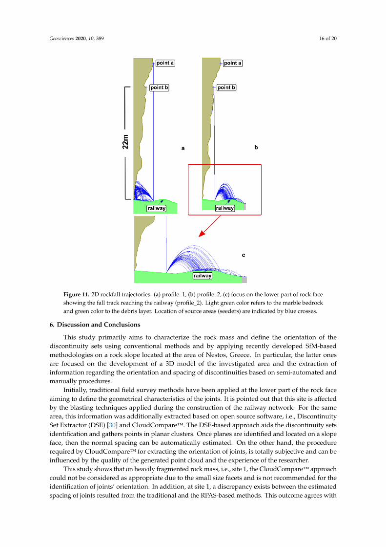
In particular, the profile_1 concerns the fall track of the block detached by point a (Figure 11a).The result of this simulation indicates that this failure cannot threaten the railway and consequentlythe rockfall hazard can be neglected. This is because after the rebound on the ground, the directionof the boulder is towards the base of the rock slope and not towards the railway. On the other hand,the profile_2 which represents the trajectory of the block detached from point b, indicates that therockfall will end up at the railway after the rebound on the ground (Figure 11b,c).

The maximum total kinetic energy of the rockfall (profile_2) at the location of the impact with theground is 134 kJ while the maximum height of the rockfall after the rebound occurs in a distance of 5 mfrom the base of the rock slope and was estimated as 3.6 m. At this location, the maximum value of thekinetic energy was estimated as 9.3 kJ, while the probability of a boulder to exceed the 5 kJ of the totalkinetic energy is approximately 15% (8 of 50 blocks used as a sample). The relevant value of a boulderto reach the height of 2 m is less than 30% (14 of 50 blocks).

Geosciences 2020, 10, 389 16 of 20

Geosciences 2020, 10, x FOR PEER REVIEW 15 of 19

In particular, the profile_1 concerns the fall track of the block detached by point a (Figure 11a). The result of this simulation indicates that this failure cannot threaten the railway and consequently the rockfall hazard can be neglected. This is because after the rebound on the ground, the direction of the boulder is towards the base of the rock slope and not towards the railway. On the other hand, the profile_2 which represents the trajectory of the block detached from point b, indicates that the rockfall will end up at the railway after the rebound on the ground (Figure 11b,c).

Figure 11. 2D rockfall trajectories. (a) profile_1, (b) profile_2, (c) focus on the lower part of rock face showing the fall track reaching the railway (profile_2). Light green color refers to the marble bedrock and green color to the debris layer. Location of source areas (seeders) are indicated by blue crosses.

The maximum total kinetic energy of the rockfall (profile_2) at the location of the impact with the ground is 134 kJ while the maximum height of the rockfall after the rebound occurs in a distance of 5 m from the base of the rock slope and was estimated as 3.6 m. At this location, the maximum value of the kinetic energy was estimated as 9.3 kJ, while the probability of a boulder to exceed the 5 kJ of the total kinetic energy is approximately 15% (8 of 50 blocks used as a sample). The relevant value of a boulder to reach the height of 2 m is less than 30% (14 of 50 blocks).

6. Discussion and Conclusions

This study primarily aims to characterize the rock mass and define the orientation of the discontinuity sets using conventional methods and by applying recently developed SfM-based methodologies on a rock slope located at the area of Nestos, Greece. In particular, the latter ones are focused on the development of a 3D model of the investigated area and the extraction of information regarding the orientation and spacing of discontinuities based on semi-automated and manually procedures.

Figure 11. 2D rockfall trajectories. (a) profile_1, (b) profile_2, (c) focus on the lower part of rock faceshowing the fall track reaching the railway (profile_2). Light green color refers to the marble bedrockand green color to the debris layer. Location of source areas (seeders) are indicated by blue crosses.

6. Discussion and Conclusions

This study primarily aims to characterize the rock mass and define the orientation of thediscontinuity sets using conventional methods and by applying recently developed SfM-basedmethodologies on a rock slope located at the area of Nestos, Greece. In particular, the latter onesare focused on the development of a 3D model of the investigated area and the extraction ofinformation regarding the orientation and spacing of discontinuities based on semi-automated andmanually procedures.

Initially, traditional field survey methods have been applied at the lower part of the rock faceaiming to define the geometrical characteristics of the joints. It is pointed out that this site is affectedby the blasting techniques applied during the construction of the railway network. For the samearea, this information was additionally extracted based on open source software, i.e., DiscontinuitySet Extractor (DSE) [30] and CloudCompare™. The DSE-based approach aids the discontinuity setsidentification and gathers points in planar clusters. Once planes are identified and located on a slopeface, then the normal spacing can be automatically estimated. On the other hand, the procedurerequired by CloudCompare™ for extracting the orientation of joints, is totally subjective and can beinfluenced by the quality of the generated point cloud and the experience of the researcher.

This study shows that on heavily fragmented rock mass, i.e., site 1, the CloudCompare™ approachcould not be considered as appropriate due to the small size facets and is not recommended for theidentification of joints’ orientation. In addition, at site 1, a discrepancy exists between the estimatedspacing of joints resulted from the traditional and the RPAS-based methods. This outcome agrees with

Geosciences 2020, 10, 389 17 of 20

the conclusion of [30] that more clusters can be detected based on the point cloud-based approach,resulting to a smaller spacing between the discontinuity sets, compared to the ones measured duringtraditional investigation. Regarding the classification of the rock mass, the DSE-based characterizationslightly differs from the one performed based on the information provided by the field survey.This difference is due to the fact that the structural analysis performed by DSE is more detailed incomparison to the coarser analysis that is conducted during field survey in accessible zones.

Therefore, at reachable heavily fragmented rock masses, it is suggested to initially perform adetailed field survey that can be used as core data and afterwards conduct a structural analysis basedon the developed 3D point-cloud, using open source software, i.e., Discontinuity Set Extractor, DSE,in order to define the orientation of the discontinuity sets (DS) and to estimate the joint spacing.

Considering the second site, it was concluded that both DSE and CloudCompare™ extractedsimilar information regarding the orientation of discontinuity sets. This probably happens becausethis area is free of human activities, and consequently not so fragmented as the one at the lower part ofthe slope. Thus, at the areas that are not reachable due to steep morphology and where conventionalmethods cannot be applied, the point-cloud approaches should be used for the rock mass classificationand the identification of the orientation of discontinuity sets. At the zones where planar surfacescan clearly be defined, CloudCompare™ could be accurately define the dominant discontinuity setsand can be additionally used for validating the orientation of joints. However, comparing to DSE,the extraction of this information is considered as time consuming.

Combining the information collected during traditional field survey and the data extracted fromthe generated 3D model, rock mass characterization was realized based on classification developedby [2], i.e., RMR and afterwards the slope mass rating (SMR) was assigned.

The secondary goal of this research was the assessment of rockfall hazard and the evaluationof critical parameters of the fall. In order to achieve this, we used the developed 3D model of theslope face for detecting and estimating the volume of potentially unstable blocks. This procedure canbe performed using the relevant tool on CloudCompare™while the accuracy of the obtained blockdimensions strongly depends on the quality of the point cloud.

In this case study, two source areas were identified and the characteristics of the likely to occurrockfalls were evaluated. Considered the results of the simulation, it is concluded that only one ofthe two examined fall tracks can threat the railway line. The proximity of the rail network to the rockslope and the type of rockfall, i.e., free fall, indicate that construction of a rockfall barrier or a rock shedare the recommended protection measures. However, scaling is suggested as the primary mitigationmeasure that should be realized in advance in order to minimize the risk.

Author Contributions: Project design, methodology, structural analysis, validation, field work, writing—originaldraft preparation, writing—review and editing, G.P.; software, validation, writing—original draft preparation,writing—review and editing, A.R.; field work, T.T.; field work, E.E. All authors have read and agreed to thepublished version of the manuscript.

Funding: This work was partially funded by the University of Alicante (vigrob-157 and GRE18-05Projects), the Spanish Ministry of Economy and Competitiveness (MINECO) and EU FEDER underProject TEC2017-85244-C2-1-P.

Acknowledgments: We would like to thank the two anonymous reviewers for their constructive commentsand suggestions.

Conflicts of Interest: The authors declare no conflict of interest.

References

1. Scavia, C.; Barbero, M.; Castelli, M.; Marchelli, M.; Peila, D.; Torsello, G.; Vallero, G. Evaluating Rockfall Risk:Some Critical Aspects. Geosciences 2020, 10, 98. [CrossRef]

2. Bieniawski, Z.T. Engineering Rock Mass Classifications: A Complete Manual for Engineers and Geologists in Mining,Civil, and Petroleum Engineering; John Wiley & Sons: Hoboken, NJ, USA, 1989.

Geosciences 2020, 10, 389 18 of 20

3. Barton, N.R.; Lien, R.; Lunde, J. Engineering classification of rock masses for the design of tunnel support.Rock Mech. 1974, 6, 189–239. [CrossRef]

4. Marinos, P.; Hoek, E. Estimating the geotechnical properties of heterogeneous rock masses such as flysch.Bull. Eng. Geol. Environ. 2001, 60, 85–92. [CrossRef]

5. Hoek, E.; Marinos, P.; Marinos, V. Characterization and engineering properties of tectonically undisturbedbut lithologically varied sedimentary rock masses. Int. J. Rock Mech. Min. Sci. 2005, 42, 277–285. [CrossRef]

6. Hoek, E. Practical Rock Engineering; Rocscience: Toronto, ON, Canada, 2006; p. 341.7. Varnes, D.J. Slope movements types and processes. In Landsllide Analysis and Control; Schruster, R.L.,

Krizek, R.J., Eds.; Transportation Research Board: Washington, DC, USA, 1978; Volume 176, pp. 11–33.8. Volkwein, A.; Schellenberg, K.; Labiouse, V.; Agliardi, F.; Berger, F.; Bourrier, F.; Dorren, L.K.A.; Gerber, V.;

Jaboyedoff, M. Rockfall characterisation andstructural protection—A review. Nat. Hazards Earth Syst. Sci.2011, 11, 2617–2651. [CrossRef]

9. Guzzetti, F.; Crosta, G.; Detti, R.; Agliardi, F. STONE: A computer programm for the three-dimensionalsimulation of rock-falls. Comput. Geosci. 2002, 28, 1079–1093. [CrossRef]

10. Rouiller, J.D.; Jaboyedoff, M.; Marro, C.; Philippossian, F.; Mamin, M. Rapport final du programme nationalde Recherche PNR 31/CREALP. In Pentes Instables dans le Pennique Valaisan; VDF Hochschulverlag AG: Zurich,Switzerland, 1998; Volume 98, p. 239.

11. Dorren, L.K.A. A review of rockfall mechanics and modelling approaches. Progr. Phys. Geogr. 2003, 27, 69–87.[CrossRef]

12. Mignelli, C.; Russo, S.L.; Peila, D. ROckfall risk MAnagement assessment: The RO.MA. approach. Nat. Hazards2012, 62. [CrossRef]

13. Ferlisi, S.; Cascini, L.; Corominas, J.; Matano, F. Rockfall risk assessment to persons travelling in vehiclesalong a road: The case study of the Amalfi coastal road (southern Italy). Nat. Hazards 2012, 62. [CrossRef]

14. Macciotta, R.; Martin, C.; Edwards, T.; Cruden, D.M.; Keegan, T. Quantifying weather conditions for rock fallhazard management. Georisk 2015, 9, 171–186. [CrossRef]

15. Macciotta, R.; Martin, D.; Morgenstern, N.; Cruden, D. Quantitative Risk Assessment of Slope Hazards alonga Section of Railway in the Canadian Cordillera–A Methodology Considering the Uncertainty in the Results.Landslides 2016, 13. [CrossRef]

16. Sala, Z.; Hutchinson, D.J.; Harrap, R. Simulation of fragmental rockfalls detected using terrestrial laser scansfrom rock slopes in south-central British Columbia, Canada. Nat. Hazards Earth Syst. Sci. 2019, 19, 2385–2404.[CrossRef]

17. Turner, A.K.; Jayaprakash, G.P. Introduction. In Rockfall Characterization and Control; Turner, A.K.,Schuster, R.L., Eds.; Transportation Research Board, National Academy of Sciences: Washington, DC,USA, 2012; pp. 3–20.

18. Nguyen, H.T.; Fernandez-Steeger, T.M.; Wiatr, T.; Rodrigues, D.; Azzam, R. Use of terrestrial laser scanningfor engineering geological applications on volcanic rock slopes—An example from Madeira island (Portugal).Nat. Hazards Earth Syst. Sci. 2011, 11, 807. [CrossRef]

19. Abellán, A.; Oppikofer, T.; Jaboyedoff, M.; Rosser, N.J.; Lim, M.; Lato, M.J. Terrestrial laser scanning of rockslope instabilities. Earth Surf. Process. Landf. 2013, 39, 80–97. [CrossRef]

20. Colomina, I.; Molina, P. Unmanned aerial systems for photogrammetry and remote sensing: A review.ISPRS J. Photogramm. Remote. Sens. 2014, 92, 79–97. [CrossRef]

21. Lindner, G.; Schraml, K.; Mansberger, R.; Hübl, J. UAV monitoring and documentation of a large landslide.Appl. Geomat. 2016, 8, 1–11. [CrossRef]

22. Rossi, G.; Tanteri, L.; Tofani, V.; Vannoci, P.; Moretti, S.; Casagli, N. Use of multicopter drone optical imagesfor landslide mapping and characterization. Nat. Hazards Earth Syst. Sci. Discuss. 2017. [CrossRef]

23. Giordan, D.; Hayakawa, Y.; Nex, F.; Remondino, F.; Tarolli, P. Review article: The use of remotely pilotedaircraft systems (RPASs) for natural hazards monitoring and management. Nat. Hazards Earth Syst. Sci. 2018,18, 1079–1096. [CrossRef]

24. Yu, M.; Huang, Y.; Zhou, J.; Mao, L. Modeling of landslide topography based on micro-unmanned aerialvehicle photography and structure-from-motion. Environ. Earth Sci. 2017, 76, 520. [CrossRef]

25. Karantanellis, E.; Marinos, V.; Vassilakis, E.; Christaras, B. Object-Based Analysis Using Unmanned AerialVehicles (UAVs) for Site-Specific Landslide Assessment. Remote Sens. 2020, 12, 1711. [CrossRef]

Geosciences 2020, 10, 389 19 of 20

26. Valkaniotis, S.; Papathanassiou, G.; Ganas, A. Mapping an earthquake-induced landslide based on UAVimagery; case study of the 2015 Okeanos landslide, Lefkada, Greece. Eng. Geol. 2018, 245, 141–152. [CrossRef]

27. Buyer, A.; Schubert, W. Calculation the Spacing of Discontinuities from 3D Point Clouds. Procedia Eng. 2017,191, 270–278. [CrossRef]

28. Sarro, R.; Riquelme, A.; García, G.H.; Mateos, R.M.; Tomàs, R.; Pastor, J.L.; Cano, M.; Herrera, G. RockfallSimulation Based on UAV Photogrammetry Data Obtained during an Emergency Declaration: Applicationat a Cultural Heritage Site. Remote Sens. 2018, 10, 1923. [CrossRef]

29. Riquelme, A.; Tomás, R.; Abellán, A. A calculator for determining Slope Mass Rating (SMR). In SMRTool Beta;Universidad de Alicante: Alicante, Spain, 2014. Available online: http://personal.ua.es/es/ariquelme/smrtool.html (accessed on 27 September 2020).

30. Riquelme, A.J.; Abellán, A.; Tomàs, R. Discontinuity spacing analysis in rock masses using 3D point clouds.Eng. Geol. 2015, 195, 185–195. [CrossRef]

31. Riquelme, A.; Tomàs, R.; Cano, M.; Pastor, J.L.; Abellán, A. Automatic Mapping of Discontinuity Persistenceon Rock Masses Using 3D Point Clouds. Rock Mech. Rock Eng. 2018, 51, 3005–3028. [CrossRef]

32. ISRM (International Society for Rock Mechanics). Suggested methods for the quantitative description ofdiscontinuities in rock masses. Int. J. Rock Mech. Min. Sci. Geomech. 1978, 16, 22.

33. Gigli, G.; Morelli, S.; Fornera, S.; Casagli, N. Terrestrial laser scanner and geomechanical surveys for therapid evaluation of rock fall susceptibility scenarios. Landslides 2012, 11, 1–14. [CrossRef]

34. Francioni, M.; Stead, D.; Sciarra, N.; Calamita, F. A new approach for defining Slope Mass Rating inheterogeneous sedimentary rocks using a combined remote sensing GIS approach. Bull. Eng. Geol. Environ.2018, 78, 4253–4274. [CrossRef]

35. Vanneschi, C.; Di Camillo, M.; Aiello, E.; Bonciani, F.; Salvini, R. SfM-MVS Photogrammetry for rockfallhazard analysis and hazard assessment along the ancient roma via flamina road at the Furlo gorge (Italy).ISPRS Int. J. Geo Inf. 2019, 8, 325. [CrossRef]

36. Pérez-Rey, I.; Riquelme, A.; Santos, L.M.G.-d.; Estévez-Ventosa, X.; Tomás, R.; Alejano, L.R. A multi-approachrockfall hazard assessment on a weathered granite natural rock slope. Landslides 2019, 16, 2005–2015.[CrossRef]

37. Riquelme, A.J.; Roberto, T.; Abellán, A. Characterization of rock slopes through slope mass rating using 3Dpoint clouds. Int. J. Rock Mech. Min. Sci. 2016, 84. [CrossRef]

38. Francioni, M.; Simone, M.; Stead, D.; Sciarra, N.; Mataloni, G.; Calamita, F. A New Fast and Low-CostPhotogrammetry Method for the Engineering Characterization of Rock Slopes. Remote Sens. 2019, 11, 1267.[CrossRef]

39. Kronberg, P.; Eltgen, H. Map sheet Xanthi. In Geological Map of Greece in 1:50.000 Scale; Institute of Geologicaland Mining Exploration: Athens, Greece, 1973.

40. Palmström, A. The volumetric joint count–A useful and simple measure of the degree of rock jointing.In Proceedings of the 4th International Congress, International Association of Engineering Geology, Delhi,India, 22–23 August 1982; Volume 5, pp. 221–228.

41. Botev, Z.I.; Grotowski, J.F.; Kroese, D.P. Kernel density estimation via diffusion. Ann. Stat. 2010, 38, 2916–2957.Available online: https://projecteuclid.org/euclid.aos/1281964340 (accessed on 27 September 2020). [CrossRef]

42. Ester, M.; Kriegel, H.-P.; Sander, J.; Xu, X. A Density-Based Algorithm for Discovering Clusters in Large SpatialDatabases with Noise; KDD: Munich, Germany, 1996; pp. 226–231.

43. Palmström, A. Measurement and Characterization of Rock Mass Jointing; A.A. Balkema Publishers: Tokyo,Japan, 2001.

44. Cai, M.; Kaiser, P.K.; Uno, H.; Tasaka, Y.; Minami, M. Estimation of rock mass strength and deformationmodulus of jointed hard rock masses using the GSI system. Int. J. Rock Mech. Min. Sci. 2004, 41, 3–19.[CrossRef]

45. Romana, M.A. Geomechanical classification for slopes: Slope mass rating. Compr. Rock Eng. 1985, 3, 575–599.46. Romana, M.; Serón, J.; Montalar, E. SMR Geomechanics classification: Application, experience and validation.

In Proceedings of the 10th ISRM Congress, Sandtoun, South Africa, 8–12 September 2003; pp. 981–984.47. Romana, M. SMR classification. In Proceedings of the 7th ISRM International Congress on Rock Mechanics, Aachen,

Germany, 16–20 September 1991; A A Balkema: Rotterdam, The Netherlands, 1991; Volume 2, pp. 955–960,Int. J. Rock Mech. Min. Sci. Geomech. Abstr. 1993, 30, A231–A231.

Geosciences 2020, 10, 389 20 of 20

48. Tomás, R.; Delgado, J.; Serón, J. Modification of slope mass rating (SMR) by continuous functions. Int. J. RockMech. Min. Sci. 2007, 44, 1062–1069. [CrossRef]

49. Pastor, J.L.; Riquelme, A.J.; Tomás, R.; Cano, M. Clarification of the slope mass rating parameters assisted bySMRTool, an open-source software. Bull. Eng. Geol. Environ. 2019, 78, 6131–6142. [CrossRef]

50. Romana, M.; Tomás, R.; Serón, J.B. Slope Mass Rating (SMR) geomechanics classification: Thirty years review.In Proceedings of the ISRM Congress 2015 International Symposium on Rock Mechanics, Montreal, QC,Canada, 10–13 May 2015; International Society for Rock Mechanics and Rock Engineering: Lisbon, Portugal,2015; p. 10, ISBN 978–1-926872-25-4.

51. Stevens, W. Rocfall: A Tool for Probabilistic Analysis, Design of Remedial Measures and Prediction ofRockfalls. Master’s Thesis, Department of Civil Engineering, University of Toronto, Toronto, ON, Canada,1998; p. 105.

52. Corominas, J.; Mavrouli, O.; Ruiz-Carulla, R. Advancing Culture of Living with Landslides. In RockfallOccurrence and Fragmentation; Sassa, K., Mikoš, M., Yin, Y., Eds.; Springer: Cham, Switzerland, 2017.

© 2020 by the authors. Licensee MDPI, Basel, Switzerland. This article is an open accessarticle distributed under the terms and conditions of the Creative Commons Attribution(CC BY) license (http://creativecommons.org/licenses/by/4.0/).