rock: a robust clustering algorithm for categorical attributes · rock: a robust clustering...
TRANSCRIPT
ROCK: A Robust Clustering Algorithm for
Categorical Attributes
S. Guha, R. Rastogi and K. Shim
S. Guha, R. Rastogi and K. Shim ROCK Mark Harrison and John-Paul Cunliffe
1
Introduction
• Clustering, traditional approaches.
• The ROCK algorithm.
• Experiments.
– Artificial dataset.– Real-world datasets.
S. Guha, R. Rastogi and K. Shim ROCK Data Mining and Exploration, 2007
2
Aim: Cluster Items with non-Numerical Attributes
• Clustering: Group similar items together, keep disimilar items apart.
• We are interested in clustering based on non-numerical data—catagorical/boolean attributes.
Catagorical: { black, white, red, green, blue }Boolean: { true, false }
• Boolean attributes are mearly a special case of catagorical attributes.
S. Guha, R. Rastogi and K. Shim ROCK Data Mining and Exploration, 2007
3
An Example Problem
• Supermarket transactions.
• Each datapoint represents the set of items bought by a single customer.
• We wish to group customers so that those buying similiar types of items appearin the same group, e.g:Group A— baby-related: diapers, baby-food, toys.Group B— expensive imported foodstuffs.etc...
• Reperesent each transaction as a binary vector in which each attributereperesents the presence or absence of a particular item in the transaction(boolean).
S. Guha, R. Rastogi and K. Shim ROCK Data Mining and Exploration, 2007
4
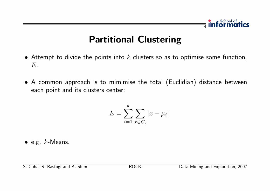
Partitional Clustering
• Attempt to divide the points into k clusters so as to optimise some function,E.
• A common approach is to mimimise the total (Euclidian) distance betweeneach point and its clusters center:
E =k∑
i=1
∑
x∈Ci
|x − µi|
• e.g. k-Means.
S. Guha, R. Rastogi and K. Shim ROCK Data Mining and Exploration, 2007
5
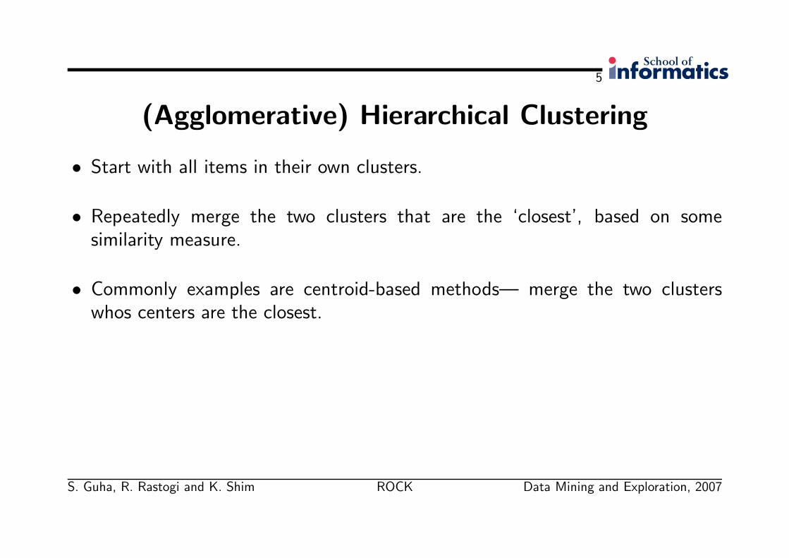
(Agglomerative) Hierarchical Clustering
• Start with all items in their own clusters.
• Repeatedly merge the two clusters that are the ‘closest’, based on somesimilarity measure.
• Commonly examples are centroid-based methods— merge the two clusterswhos centers are the closest.
S. Guha, R. Rastogi and K. Shim ROCK Data Mining and Exploration, 2007
6
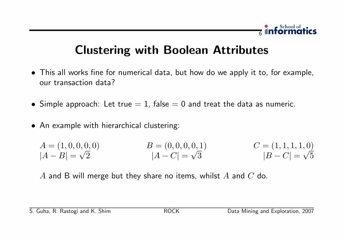
Clustering with Boolean Attributes
• This all works fine for numerical data, but how do we apply it to, for example,our transaction data?
• Simple approach: Let true = 1, false = 0 and treat the data as numeric.
• An example with hierarchical clustering:
A = (1, 0, 0, 0, 0) B = (0, 0, 0, 0, 1) C = (1, 1, 1, 1, 0)|A − B| =
√2 |A − C| =
√3 |B − C| =
√5
A and B will merge but they share no items, whilst A and C do.
S. Guha, R. Rastogi and K. Shim ROCK Data Mining and Exploration, 2007
7
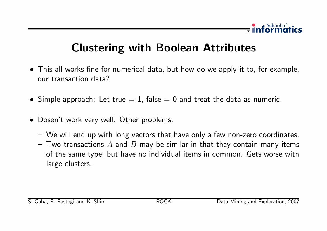
Clustering with Boolean Attributes
• This all works fine for numerical data, but how do we apply it to, for example,our transaction data?
• Simple approach: Let true = 1, false = 0 and treat the data as numeric.
• Dosen’t work very well. Other problems:
– We will end up with long vectors that have only a few non-zero coordinates.– Two transactions A and B may be similar in that they contain many items
of the same type, but have no individual items in common. Gets worse withlarge clusters.
S. Guha, R. Rastogi and K. Shim ROCK Data Mining and Exploration, 2007
8
Clustering with Boolean Attributes
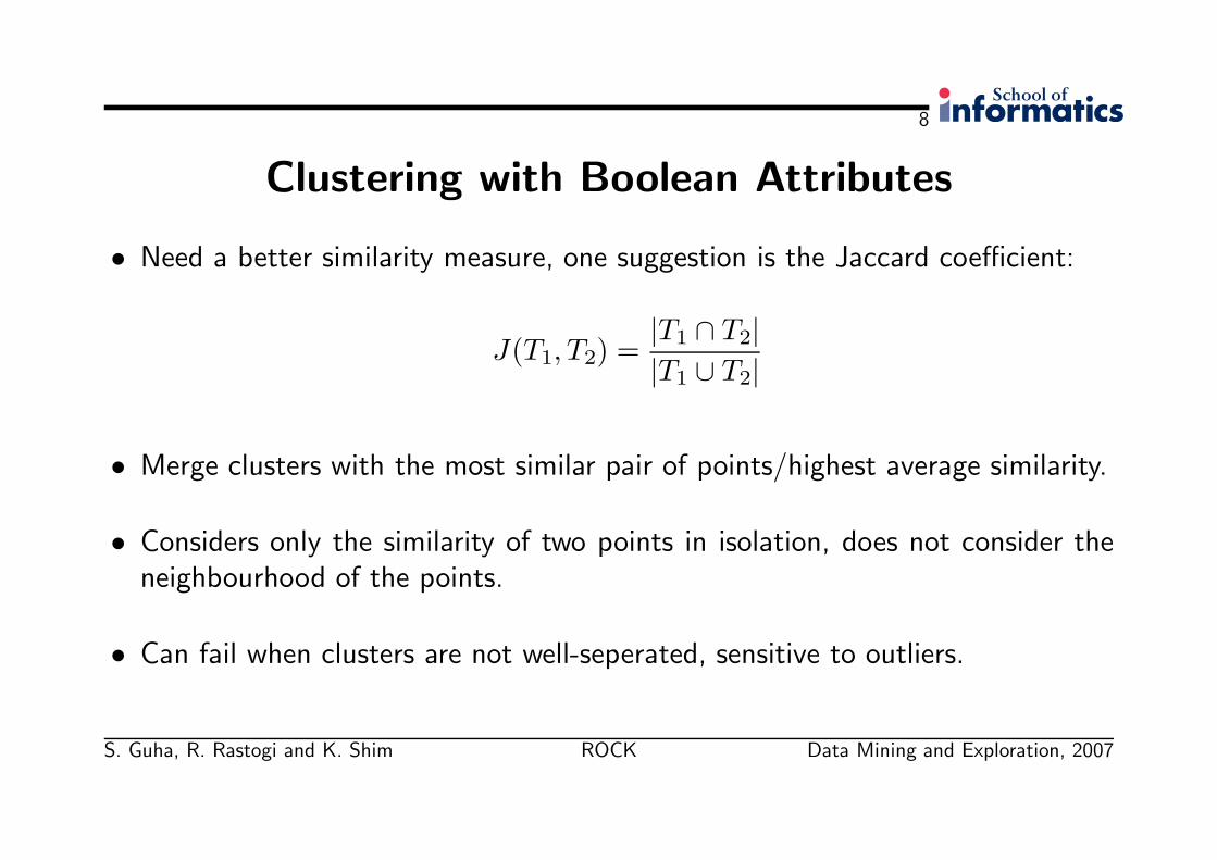
• Need a better similarity measure, one suggestion is the Jaccard coefficient:
J(T1, T2) =|T1 ∩ T2||T1 ∪ T2|
• Merge clusters with the most similar pair of points/highest average similarity.
• Considers only the similarity of two points in isolation, does not consider theneighbourhood of the points.
• Can fail when clusters are not well-seperated, sensitive to outliers.
S. Guha, R. Rastogi and K. Shim ROCK Data Mining and Exploration, 2007
9
Neighbours and Links
• Need a more global approach that considers the links between points.
• Use common neighbours to define links.
• If point A neighbours point C, and point B neighbours point C then thepoints A and B are linked, even if they are not themselves neighbours.
• If two points belong to the same cluster they should have many commonneighbours.
• If they belong to different clusters they will have few common neighbours.
S. Guha, R. Rastogi and K. Shim ROCK Data Mining and Exploration, 2007
10
Neighbours and Links
• We need a way of deciding which points are ‘neighbours’.
• Define a similarity function, sim(p1, p2), that encodes the level of similarity(’closeness’) between two points.
• Normalise so that sim(p1, p2) is one when p1 equals p2 and zero when theyare completely dissimilar.
• We then consider p1 and p2 to be ’neighbours’ if sim(p1, p2) ≥ θ, where θ isa user-provided paramater.
S. Guha, R. Rastogi and K. Shim ROCK Data Mining and Exploration, 2007
11
Neighbours and Links
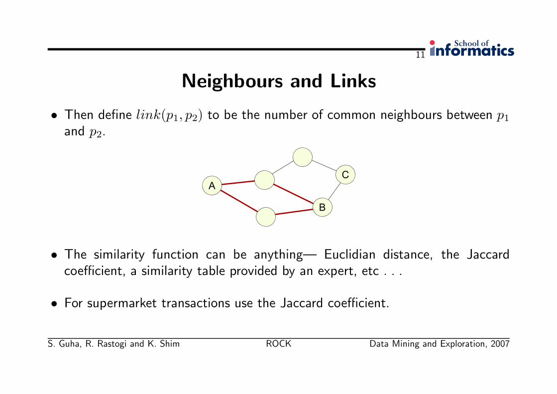
• Then define link(p1, p2) to be the number of common neighbours between p1
and p2.
• The similarity function can be anything— Euclidian distance, the Jaccardcoefficient, a similarity table provided by an expert, etc . . .
• For supermarket transactions use the Jaccard coefficient.
S. Guha, R. Rastogi and K. Shim ROCK Data Mining and Exploration, 2007
12
The Criterion Function
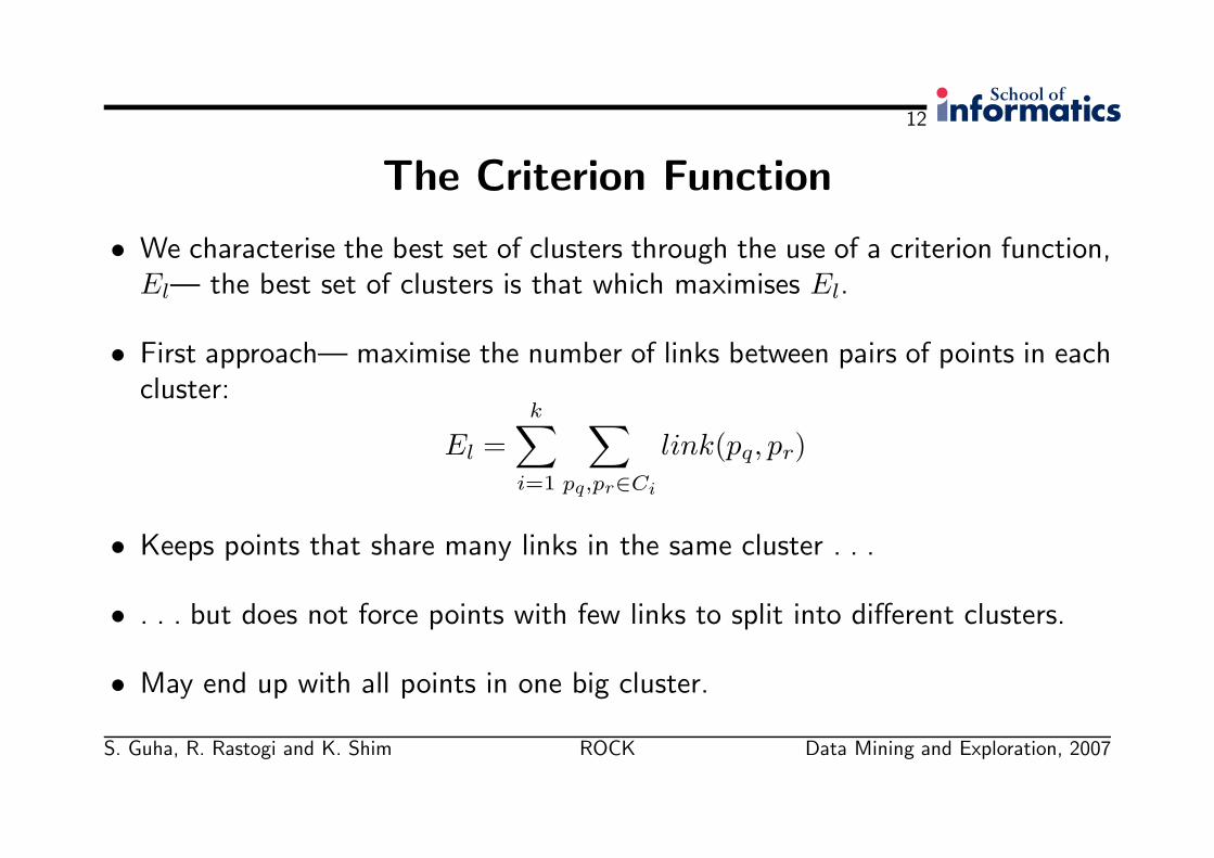
• We characterise the best set of clusters through the use of a criterion function,El— the best set of clusters is that which maximises El.
• First approach— maximise the number of links between pairs of points in eachcluster:
El =
k∑
i=1
∑
pq,pr∈Ci
link(pq, pr)
• Keeps points that share many links in the same cluster . . .
• . . . but does not force points with few links to split into different clusters.
• May end up with all points in one big cluster.
S. Guha, R. Rastogi and K. Shim ROCK Data Mining and Exploration, 2007
13
The Criterion Function
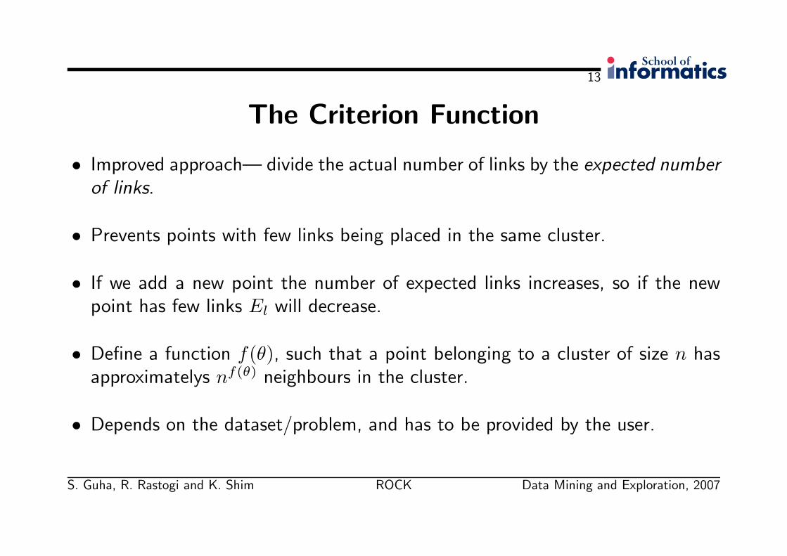
• Improved approach— divide the actual number of links by the expected number
of links.
• Prevents points with few links being placed in the same cluster.
• If we add a new point the number of expected links increases, so if the newpoint has few links El will decrease.
• Define a function f(θ), such that a point belonging to a cluster of size n hasapproximatelys nf(θ) neighbours in the cluster.
• Depends on the dataset/problem, and has to be provided by the user.
S. Guha, R. Rastogi and K. Shim ROCK Data Mining and Exploration, 2007
14
The Criterion Function
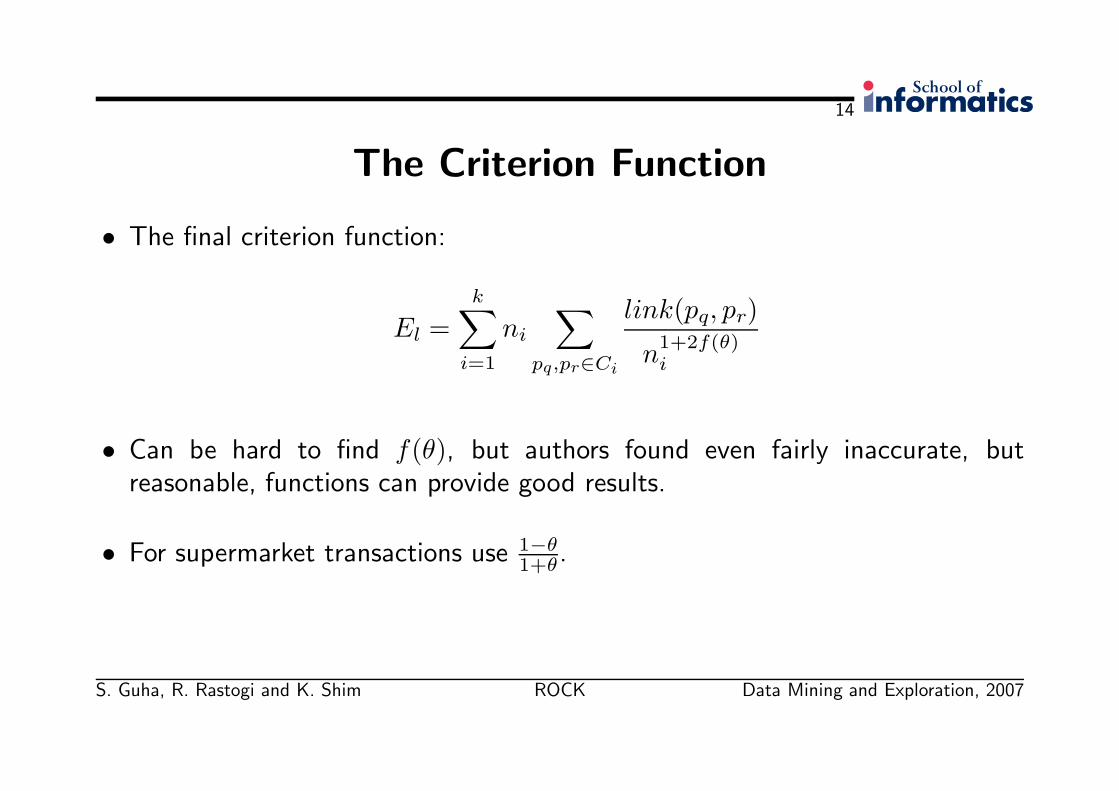
• The final criterion function:
El =k∑
i=1
ni
∑
pq,pr∈Ci
link(pq, pr)
n1+2f(θ)i
• Can be hard to find f(θ), but authors found even fairly inaccurate, butreasonable, functions can provide good results.
• For supermarket transactions use 1−θ1+θ
.
S. Guha, R. Rastogi and K. Shim ROCK Data Mining and Exploration, 2007
15
ROCK: RObust Clustering using linKs
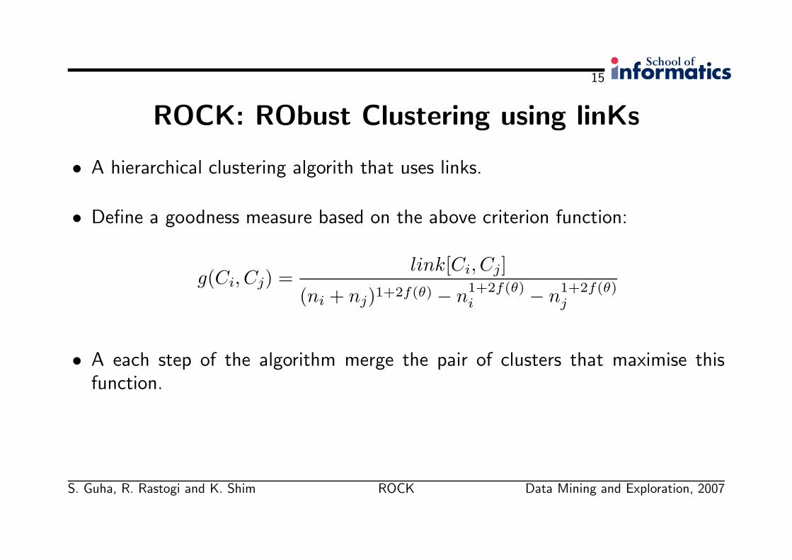
• A hierarchical clustering algorith that uses links.
• Define a goodness measure based on the above criterion function:
g(Ci, Cj) =link[Ci, Cj]
(ni + nj)1+2f(θ) − n1+2f(θ)i − n
1+2f(θ)j
• A each step of the algorithm merge the pair of clusters that maximise thisfunction.
S. Guha, R. Rastogi and K. Shim ROCK Data Mining and Exploration, 2007
16
Dealing with Catagorical Attributes
• How do we handle catagorical attributes with the possibility of missing data?
• One possible method is to convert them into transactions.
• For each attribute A and each value it can take v construct an item A.v andinclude it in the transaction if the attribute takes that value.
• If we have a missing value no item will be present.
S. Guha, R. Rastogi and K. Shim ROCK Data Mining and Exploration, 2007
17
Outliers
• Outliers will probably have very few or no neighbours, and as such will takelittle or no part in clustering and can be discarded early on.
• Small clusters of outliers will persist in isolation until near the end of clustering,so when we are close to reaching the required number of clusters we can stopand weed out any small isolated clusters with little support.
S. Guha, R. Rastogi and K. Shim ROCK Data Mining and Exploration, 2007
18
Random sampling
• If we have a huge number of points we can select a random sample with whichto do the clustering.
• Once clustering is complete we assign the remaining datapoints from diskby determining which cluster contains the most neighbours to each point(normalised by the expected number of neighbours).
S. Guha, R. Rastogi and K. Shim ROCK Data Mining and Exploration, 2007
19
Summary
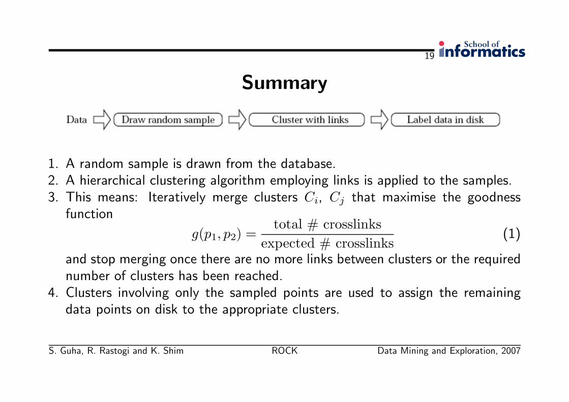
1. A random sample is drawn from the database.2. A hierarchical clustering algorithm employing links is applied to the samples.3. This means: Iteratively merge clusters Ci, Cj that maximise the goodness
function
g(p1, p2) =total # crosslinks
expected # crosslinks(1)
and stop merging once there are no more links between clusters or the requirednumber of clusters has been reached.
4. Clusters involving only the sampled points are used to assign the remainingdata points on disk to the appropriate clusters.
S. Guha, R. Rastogi and K. Shim ROCK Data Mining and Exploration, 2007
20
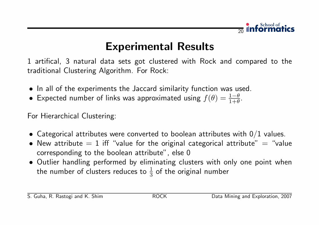
Experimental Results1 artifical, 3 natural data sets got clustered with Rock and compared to thetraditional Clustering Algorithm. For Rock:
• In all of the experiments the Jaccard similarity function was used.• Expected number of links was approximated using f(θ) = 1−θ
1+θ.
For Hierarchical Clustering:
• Categorical attributes were converted to boolean attributes with 0/1 values.• New attribute = 1 iff “value for the original categorical attribute” = “value
corresponding to the boolean attribute”, else 0• Outlier handling performed by eliminating clusters with only one point when
the number of clusters reduces to 13 of the original number
S. Guha, R. Rastogi and K. Shim ROCK Data Mining and Exploration, 2007

21
Synthetic Data Set
• Market basket database containing 114586 transactions.• Of these, 5456 (arround 5%) are outliers, while the others belong to one of 10
clusters with sizes varying between 5000 and 15000.• How did these transactions get constructed?
# Cluster 1 2 3 4 5 6
# Transactions 9736 13029 14832 10893 13022 7391# Items 19 20 19 19 22 19
# Cluster 7 8 9 10 Outliers
# Transactions 8564 11973 14279 5411 5456# Items 19 21 22 19 116
S. Guha, R. Rastogi and K. Shim ROCK Data Mining and Exploration, 2007
22
Synthetic Data Set
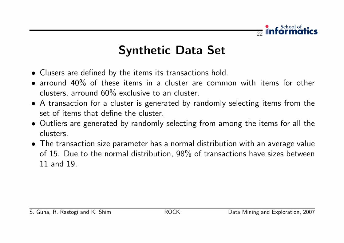
• Clusers are defined by the items its transactions hold.• arround 40% of these items in a cluster are common with items for other
clusters, arround 60% exclusive to an cluster.• A transaction for a cluster is generated by randomly selecting items from the
set of items that define the cluster.• Outliers are generated by randomly selecting from among the items for all the
clusters.• The transaction size parameter has a normal distribution with an average value
of 15. Due to the normal distribution, 98% of transactions have sizes between11 and 19.
S. Guha, R. Rastogi and K. Shim ROCK Data Mining and Exploration, 2007
23
Scalability
• Using random sampling results a greatly reduced impact of data size on theexecution time of ROCK.
• Which impact does the sample size have on the execution time (excl. labelling)?• Random sample size is varied for four different settings of θ (the “threshold of
neighbourhood”).
S. Guha, R. Rastogi and K. Shim ROCK Data Mining and Exploration, 2007
24
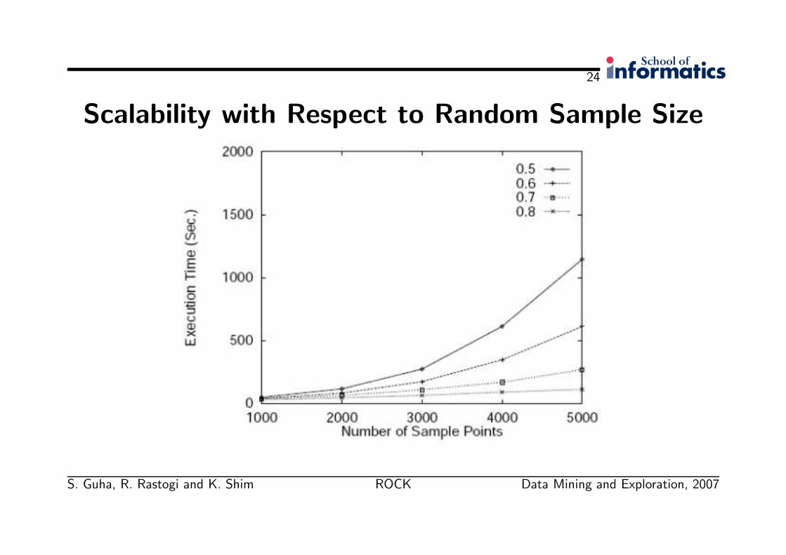
Scalability with Respect to Random Sample Size
S. Guha, R. Rastogi and K. Shim ROCK Data Mining and Exploration, 2007
25
Scalability
• The computational complexity of ROCK is roughly quadratic with respect tothe sample size.
• For a given sample size, the performance of ROCK improves as θ is increased.
• Why?
S. Guha, R. Rastogi and K. Shim ROCK Data Mining and Exploration, 2007
26
Scalability
• The computational complexity of ROCK is roughly quadratic with respect tothe sample size.
• For a given sample size, the performance of ROCK improves as θ is increased.
• Why?
• The reason for this is that as θ is increased, each transaction has fewerneighbours and this makes the computation of links more efficient.
S. Guha, R. Rastogi and K. Shim ROCK Data Mining and Exploration, 2007
27
Quality
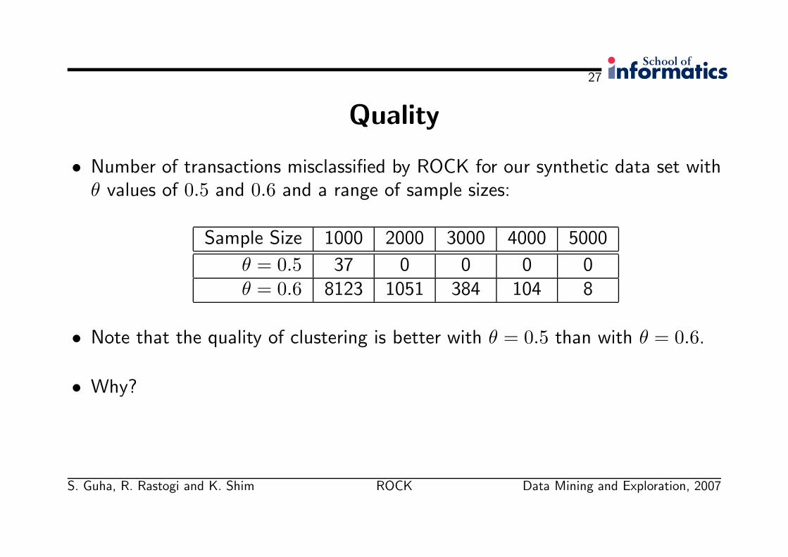
• Number of transactions misclassified by ROCK for our synthetic data set withθ values of 0.5 and 0.6 and a range of sample sizes:
Sample Size 1000 2000 3000 4000 5000
θ = 0.5 37 0 0 0 0θ = 0.6 8123 1051 384 104 8
• Note that the quality of clustering is better with θ = 0.5 than with θ = 0.6.
• Why?
S. Guha, R. Rastogi and K. Shim ROCK Data Mining and Exploration, 2007
28
Quality
• Random sample sizes we consider range from being less than 1% of thedatabase size to about 4.5%.
• Transaction sizes can be as small as 11, while the number of items definingeach cluster is approximately 20.
• A high percentage (roughly 40%) of items in a cluster are also present in otherclusters. Thus, a smaller similarity threshold is required to ensure that a largernumber of transaction pairs from the same cluster are neighbours.
S. Guha, R. Rastogi and K. Shim ROCK Data Mining and Exploration, 2007
29
Real-Life Data Sets
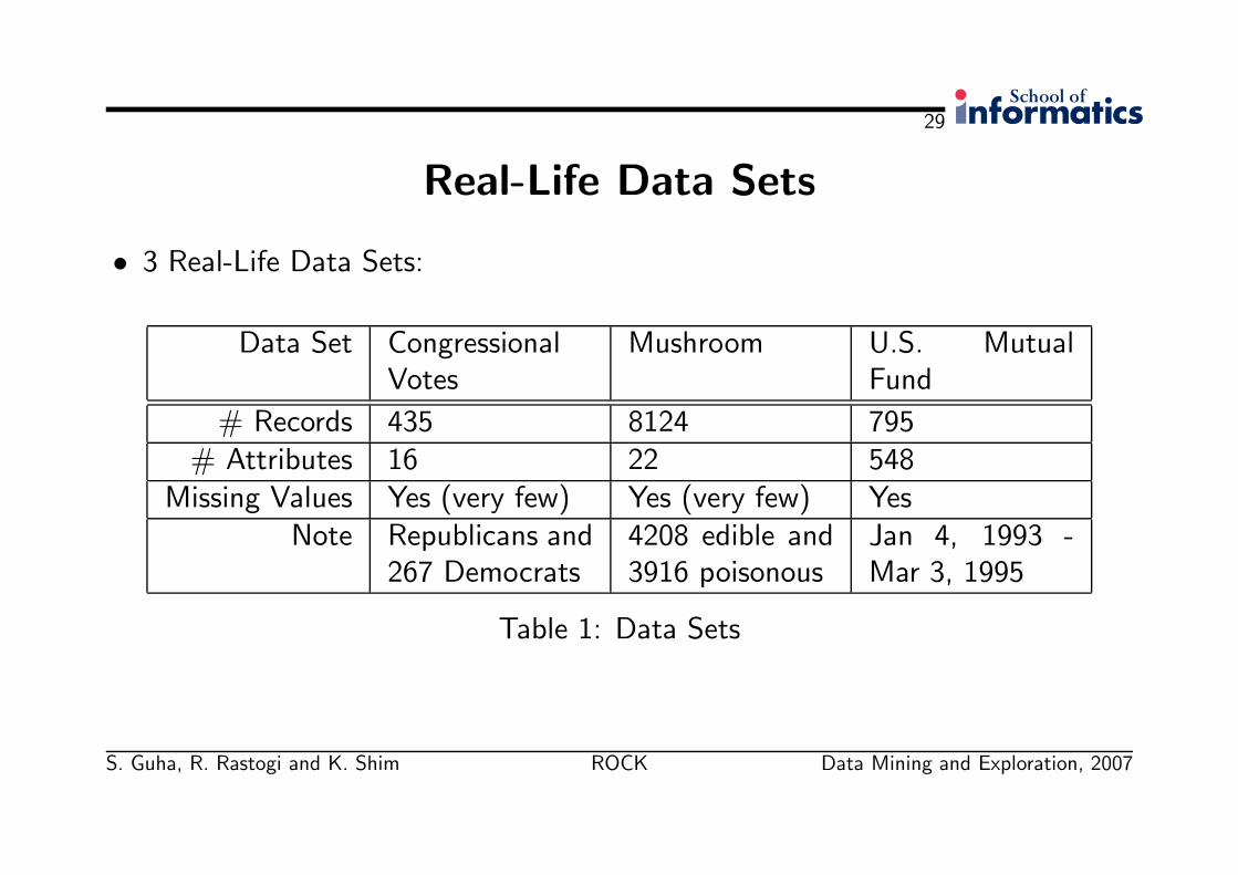
• 3 Real-Life Data Sets:
Data Set CongressionalVotes
Mushroom U.S. MutualFund
# Records 435 8124 795# Attributes 16 22 548
Missing Values Yes (very few) Yes (very few) YesNote Republicans and
267 Democrats4208 edible and3916 poisonous
Jan 4, 1993 -Mar 3, 1995
Table 1: Data Sets
S. Guha, R. Rastogi and K. Shim ROCK Data Mining and Exploration, 2007
30
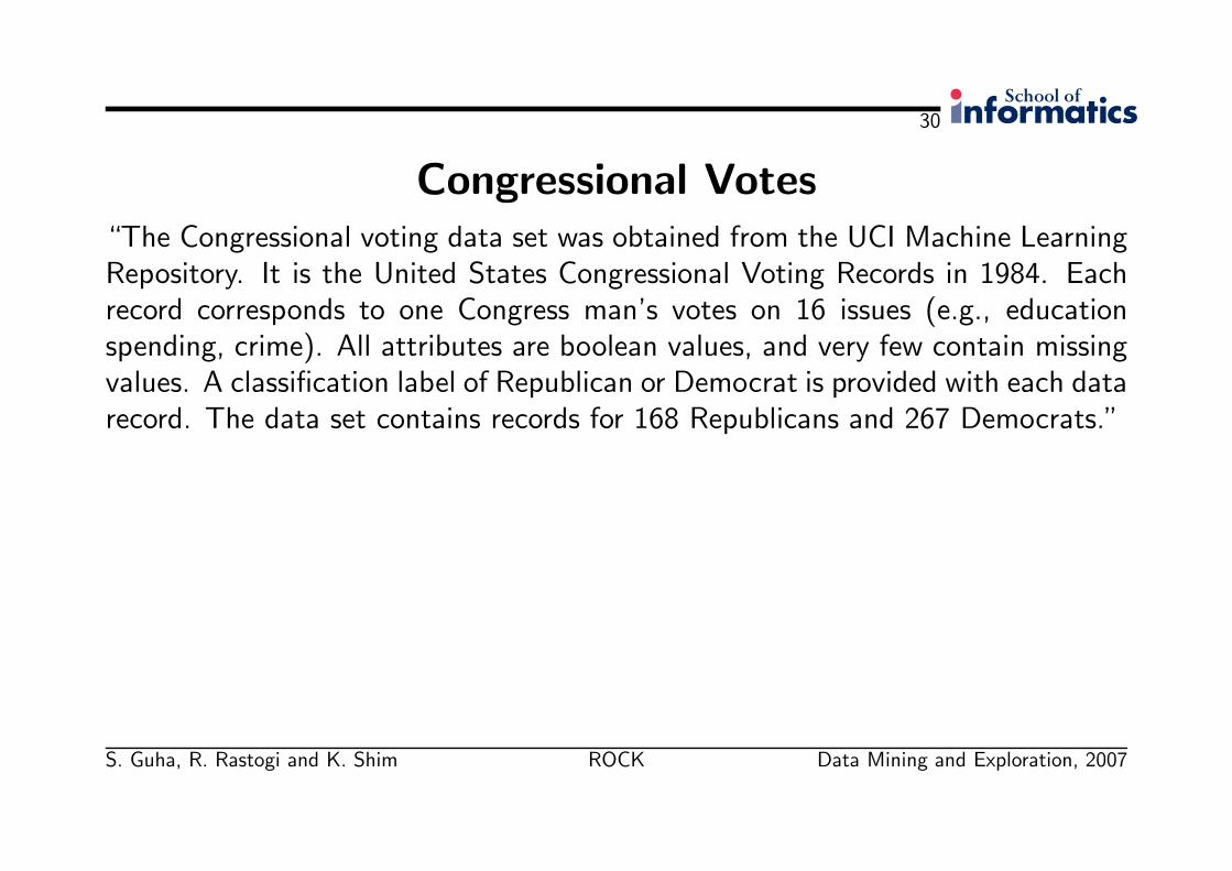
Congressional Votes“The Congressional voting data set was obtained from the UCI Machine LearningRepository. It is the United States Congressional Voting Records in 1984. Eachrecord corresponds to one Congress man’s votes on 16 issues (e.g., educationspending, crime). All attributes are boolean values, and very few contain missingvalues. A classification label of Republican or Democrat is provided with each datarecord. The data set contains records for 168 Republicans and 267 Democrats.”
S. Guha, R. Rastogi and K. Shim ROCK Data Mining and Exploration, 2007
31
Congressional Votes on the Rock
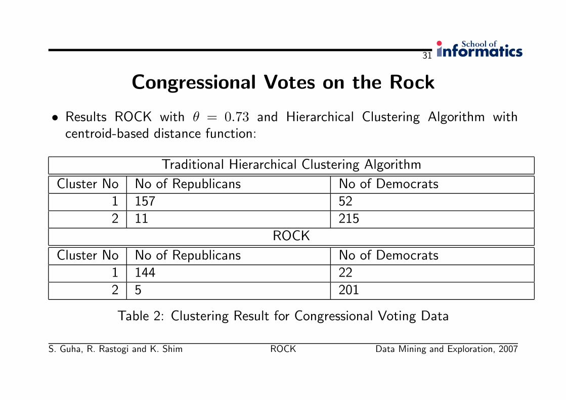
• Results ROCK with θ = 0.73 and Hierarchical Clustering Algorithm withcentroid-based distance function:
Traditional Hierarchical Clustering Algorithm
Cluster No No of Republicans No of Democrats1 157 522 11 215
ROCK
Cluster No No of Republicans No of Democrats1 144 222 5 201
Table 2: Clustering Result for Congressional Voting Data
S. Guha, R. Rastogi and K. Shim ROCK Data Mining and Exploration, 2007
32
Congressional Votes on the Rock
• Both identify two clusters one containing a large number of republicans andthe other containing a majority of democrats.
• However, in the cluster for republicans found by the traditional algorithm,around 25% of the members are democrats, while with ROCK, only 12% aredemocrats.
• Why?
S. Guha, R. Rastogi and K. Shim ROCK Data Mining and Exploration, 2007
33
Congressional Votes on the Rock
• Both identify two clusters one containing a large number of republicans andthe other containing a majority of democrats.
• However, in the cluster for republicans found by the traditional algorithm,around 25% of the members are democrats, while with ROCK, only 12% aredemocrats.
• Why?
• Improvement mainly caused by outlier removal scheme and the usage of linksby ROCK.
S. Guha, R. Rastogi and K. Shim ROCK Data Mining and Exploration, 2007
34
Congressional Votes on the RockInterestingly, the traditional algorithm also discovered the clusters easily. Reasonsfor this are:
• Only on 3 issues did a majority of Republicans and Democrats cast the samevote.
• On 12 of the remaining 13 issues, the majority of the Democrats voteddifferently from the majority of the Republicans.
• On each of the 12 issues, the Yes/No vote had sizable support in theirrespective clusters.
• Therefore the two clusters are quite well-separated.• Furthermore, there isn’t a significant difference in the sizes of the two clusters.
S. Guha, R. Rastogi and K. Shim ROCK Data Mining and Exploration, 2007
35
Mushroom“The mushroom data set was also obtained from the UCI Machine LearningRepository. Each data record contains information that describes the physicalcharacteristics (e.g., color, odor, size, shape) of a single mushroom. A recordalso contains a poisonous or edible label for the mushroom. All attributes arecategorical attributes; for instance, the values that the size attribute takes arenarrow and broad, while the values of shape can be bell, at, conical or convex, andodor is one of spicy, almond, foul, fishy, pungent etc. The mushroom databasehas the largest number of records (that is, 8124) among the real-life data sets weused in our experiments. The number of edible and poisonous mushrooms in thedata set are 4208 and 3916, respectively.”
S. Guha, R. Rastogi and K. Shim ROCK Data Mining and Exploration, 2007
36
Mushroom on the Rock
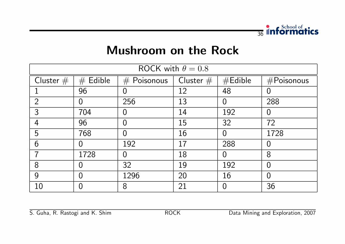
ROCK with θ = 0.8
Cluster # # Edible # Poisonous Cluster # #Edible #Poisonous1 96 0 12 48 02 0 256 13 0 2883 704 0 14 192 04 96 0 15 32 725 768 0 16 0 17286 0 192 17 288 07 1728 0 18 0 88 0 32 19 192 09 0 1296 20 16 010 0 8 21 0 36
S. Guha, R. Rastogi and K. Shim ROCK Data Mining and Exploration, 2007
37
Mushroom on the Rock
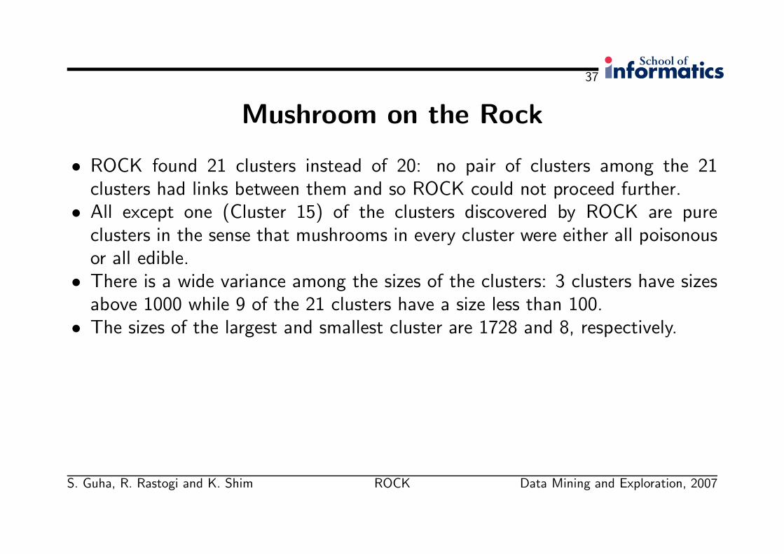
• ROCK found 21 clusters instead of 20: no pair of clusters among the 21clusters had links between them and so ROCK could not proceed further.
• All except one (Cluster 15) of the clusters discovered by ROCK are pureclusters in the sense that mushrooms in every cluster were either all poisonousor all edible.
• There is a wide variance among the sizes of the clusters: 3 clusters have sizesabove 1000 while 9 of the 21 clusters have a size less than 100.
• The sizes of the largest and smallest cluster are 1728 and 8, respectively.
S. Guha, R. Rastogi and K. Shim ROCK Data Mining and Exploration, 2007
38
Mushroom on the Rock
• In general, records in different clusters could be identical with respect to someattribute values.
• Thus, every pair of clusters generally have some common values for theattributes
• Thus clusters are not well-separated.• What does this mean for the traditional approach?
S. Guha, R. Rastogi and K. Shim ROCK Data Mining and Exploration, 2007
39
Mushroom Traditional
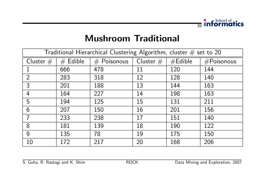
Traditional Hierarchical Clustering Algorithm, cluster # set to 20
Cluster # # Edible # Poisonous Cluster # #Edible #Poisonous1 666 478 11 120 1442 283 318 12 128 1403 201 188 13 144 1634 164 227 14 198 1635 194 125 15 131 2116 207 150 16 201 1567 233 238 17 151 1408 181 139 18 190 1229 135 78 19 175 15010 172 217 20 168 206
S. Guha, R. Rastogi and K. Shim ROCK Data Mining and Exploration, 2007
40
Mushroom on the RockObserving these results we find that:
• Points belonging to different clusters are merged into a single cluster and largeclusters are split into smaller ones
• None of the clusters generated by the traditional algorithm are pure.• Every cluster contains a sizable number of both poisonous and edible
mushrooms• Sizes of clusters detected by traditional hierarchical clustering are fairly uniform:
More than 90% of the clusters have sizes between 200 and 400, and only 1cluster has more than 1000 mushrooms.
S. Guha, R. Rastogi and K. Shim ROCK Data Mining and Exploration, 2007
41
Mushroom on the RockSo the quality of the clusters generated by the traditional algorithm was verypoor. Reasons for this are:
• Clusters are not well-separated and there is a wide variance in the sizes ofclusters.
• Cluster centers tend to spread out in all the attribute values and lose informationabout points in the cluster that they represent.
• Thus - as discussed earlier - distances between centroids of clusters become apoor estimate of the similarity between them.
S. Guha, R. Rastogi and K. Shim ROCK Data Mining and Exploration, 2007
42
US Mutual Funds“We ran ROCK on a time-series database of the closing prices of U.S. mutual fundsthat were collected from the MIT AI Laboratories’ Experimental Stock MarketData Servery. The funds represented in this dataset include bond funds, incomefunds, asset allocation funds, balanced funds, equity income funds, foreign stockfunds, growth stock funds, aggressive growth stock funds and small companygrowth funds. The closing prices for each fund are for business dates only. Someof the mutual funds that were launched later than Jan 4, 1993 do not have aprice for the entire range of dates from Jan 4, 1993 until Mar 3, 1995. Thus,there are many missing values for a certain number of mutual funds in our dataset. (...) This makes it difficult to use the traditional algorithm since it is unclearas to how to treat the missing values in the context of traditional hierarchicalclustering.”
S. Guha, R. Rastogi and K. Shim ROCK Data Mining and Exploration, 2007
43
US Mutual Funds on the Rock
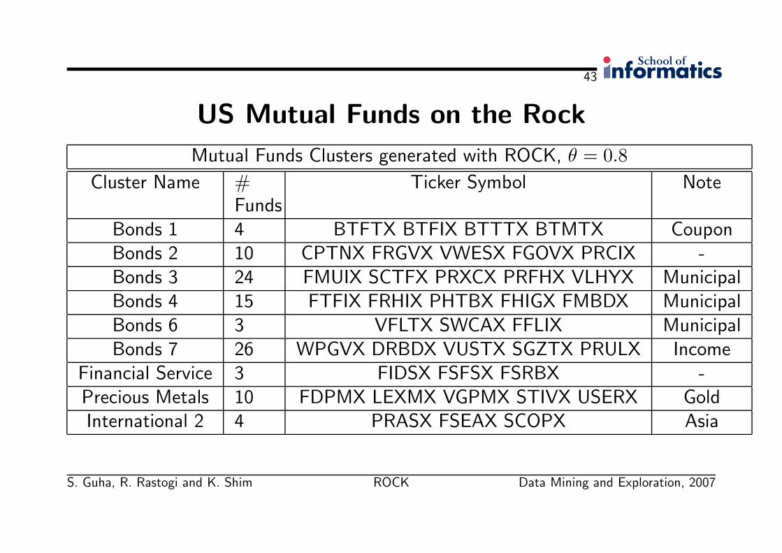
Mutual Funds Clusters generated with ROCK, θ = 0.8
Cluster Name #Funds
Ticker Symbol Note
Bonds 1 4 BTFTX BTFIX BTTTX BTMTX CouponBonds 2 10 CPTNX FRGVX VWESX FGOVX PRCIX -Bonds 3 24 FMUIX SCTFX PRXCX PRFHX VLHYX MunicipalBonds 4 15 FTFIX FRHIX PHTBX FHIGX FMBDX MunicipalBonds 6 3 VFLTX SWCAX FFLIX MunicipalBonds 7 26 WPGVX DRBDX VUSTX SGZTX PRULX Income
Financial Service 3 FIDSX FSFSX FSRBX -Precious Metals 10 FDPMX LEXMX VGPMX STIVX USERX GoldInternational 2 4 PRASX FSEAX SCOPX Asia
S. Guha, R. Rastogi and K. Shim ROCK Data Mining and Exploration, 2007
44
US Mutual Funds on the Rock
• The Financial Service cluster has 3 funds: Fidelity Select Financial Services(FIDSX), Invesco Strategic Financial Services (FSFSX) and Fidelity SelectRegional Banks (FSRBX) that invest primarily in banks, brokerages andfinancial institutions.
• The cluster named International 2 contains funds that invest in South-east Asiaand the Pacific rim region; they are T. Rowe Price New Asia (PRASX), FidelitySoutheast Asia (FSEAX), and Scudder Pacific Opportunities (SCOPX).
• The Precious Metals cluster includes mutual funds that invest mainly in Gold.
S. Guha, R. Rastogi and K. Shim ROCK Data Mining and Exploration, 2007
45
US Mutual Funds on the Rock
• It appears that ROCK can also be used to cluster time-series data.• It can be employed to determine interesting distributions in the underlying
data even when there are a large number of outliers that do not belong to anyof the clusters, as well as when the data contains a sizable number of missingvalues.
• A nice and desirable characteristic of this technique: it does not merge a pairof clusters if there are no links between them.
• Thus, the desired number of clusters input to ROCK is just a hint: ROCKmay discover more than the specified number of clusters (if there are no linksbetween clusters) or fewer (in case certain clusters are determined to be outliersand eliminated).
S. Guha, R. Rastogi and K. Shim ROCK Data Mining and Exploration, 2007
46
Remarks
• A new concept of links to measure the similarity/proximity between a pair ofdata points with categorical attributes is investiaged.
• The robust hierarchical clustering algorithm ROCK employs links and notdistances for merging clusters.
• This method naturally extend to non-metric similarity measures that arerelevant in situations where a domain expert/similarity table is the only sourceof knowledge.
• The results of the experimental study with real-life data sets is encouraging.
S. Guha, R. Rastogi and K. Shim ROCK Data Mining and Exploration, 2007
47
Email & EndJohn-Paul Cunliffe wrote:(...) If there is any relevant information not covered in your paper, I wouldappreciate any hint you can give me on it so I can present your work as completeas possible. (...)
Sudipto Guha:
(...) We started out to solve a problem, I believe the problem was solved and we(I) moved on. That’s that. ROCK does work quite well in practice, I have evenseen being used on environmental data where the categories were anonymizedand the algorithm gave correct answers.
As far as I am aware other researchers have tried to take the research to the nextstep, in terms of optimizations of various factors. (...)
S. Guha, R. Rastogi and K. Shim ROCK Data Mining and Exploration, 2007