robust video transmission over lossy channels and ...robust video transmission over lossy channels...
TRANSCRIPT
Robust video transmission over lossy channels andefficient video distribution over peer-to-peer networks
Jiajun Wang
Electrical Engineering and Computer SciencesUniversity of California at Berkeley
Technical Report No. UCB/EECS-2008-152
http://www.eecs.berkeley.edu/Pubs/TechRpts/2008/EECS-2008-152.html
December 10, 2008

Copyright 2008, by the author(s).All rights reserved.
Permission to make digital or hard copies of all or part of this work forpersonal or classroom use is granted without fee provided that copies arenot made or distributed for profit or commercial advantage and that copiesbear this notice and the full citation on the first page. To copy otherwise, torepublish, to post on servers or to redistribute to lists, requires prior specificpermission.
Robust video transmission over lossy channels and efficient video
distribution over peer-to-peer networks
by
Jiajun Wang
B.S. (University of Illinois at Urbana-Champaign) 2003M.S. (University of California, Berkeley) 2006
A dissertation submitted in partial satisfaction of the
requirements for the degree of
Doctor of Philosophy
in
Engineering - Electrical Engineering and Computer Sciences
and the Designated Emphasis
in
Communication, Computation and Statistics
in the
GRADUATE DIVISION
of the
UNIVERSITY of CALIFORNIA, BERKELEY
Committee in charge:
Professor Kannan Ramchandran, ChairProfessor Avideh Zakhor
Professor Bruno Olshausen
Fall 2008

1
Abstract
Robust video transmission over lossy channels and efficient video distribution
over peer-to-peer networks
by
Jiajun Wang
Doctor of Philosophy in Engineering - Electrical Engineering and Computer
Sciences and the Designated Emphasis in Communication, Computation and
Statistics
University of California, Berkeley
Professor Kannan Ramchandran, Chair
Though technologies for video compression and client-server based video distribution
have matured, applications fueled by recent development of communication networks
pose new challenges. In this dissertation, we study two classes of video applications.
The first class is low-latency video streaming over lossy networks. Today’s
dominant codecs based on motion-compensated predictive coding, such as MPEG,
can compress videos efficiently. However, the decoded video quality is susceptible
to transmission packet losses, which occur frequently over both the Internet and
cellular networks. In order to enable robust low-latency video transmission, we adopt
a video coding framework based on information-theoretical principles of distributed
source coding. We present the theoretical foundation of a distributed source coding
based video codec as well as the practical implementations. Extensive simulations
2
demonstrate the superiority of the proposed codec over conventional robustness-
enhancing methods, such as intra refresh and forward error correction codes.
The second class is video distribution over peer-to-peer (P2P) overlay net-
works. Compared to the traditional client-server architecture, P2P technologies
can offer tremendous scalability and greatly reduce server cost. Due to the band-
width asymmetry experienced by Internet users, however, P2P systems are often-
times bottlenecked by users’ limited upload bandwidth. We propose to ease the
bottleneck by utilizing Internet users with spare upload capacity, whom we term
helpers. We present a light-weight helper protocol that is backwards-compatible
with the popular BitTorrent protocol and analyze the steady-state system perfor-
mance. We verify the efficiency and effectiveness of the proposed protocol and the
accuracy of the analysis through extensive simulations. We further extend the phi-
losophy for live video streaming. We use a simple fluid-level analysis to guide our
system design. We demonstrate that the simple analysis provides a good estimate
of system performance and verify that the proposed system can efficiently utilize
helpers’ upload bandwidth even with high peer churning through extensive simula-
tions.
Professor Kannan RamchandranDissertation Committee Chair
i
Contents
Contents i
List of Figures iii
Acknowledgements viii
1 Introduction 1
I Robust video transmission over lossy networks 6
2 Motivation and background 72.1 Video coding and distributed source coding background . . . . . . . . 10
3 Distributed source coding based robust video transmission over net-works with bursty losses 283.1 Related work . . . . . . . . . . . . . . . . . . . . . . . . . . . . . . . . 283.2 Illustrative example . . . . . . . . . . . . . . . . . . . . . . . . . . . . 333.3 System implementation . . . . . . . . . . . . . . . . . . . . . . . . . . 433.4 Simulation results . . . . . . . . . . . . . . . . . . . . . . . . . . . . . 54
4 Conclusion and future work 60
II Video distribution over collaborative peer-to-peer networks 63
5 Introduction 645.1 Peer-to-peer networking overview . . . . . . . . . . . . . . . . . . . . . 66
ii
6 Helper-assisted peer-to-peer video distribution 716.1 The BitTorrent protocol . . . . . . . . . . . . . . . . . . . . . . . . . . 726.2 Helper-assisted peer-to-peer video download . . . . . . . . . . . . . . . 746.3 Extension to live video multicast . . . . . . . . . . . . . . . . . . . . . 93
7 Conclusion and future work 112
Bibliography 114

iii
List of Figures
2.1 Simplified demonstration of motion compensated predictive coding.Each frame is broken into non-overlapping blocks. To encode eachblock, the best predictor block is located within a search range inthe reference. The displacement between the current block and thepredictor block is called motion vector. Only the difference betweenthe current block and the predictor block and the motion vector aretransmitted. . . . . . . . . . . . . . . . . . . . . . . . . . . . . . . . . . 11
2.2 An example of a group of pictures (GOP). Every GOP starts with anI-frame. It is followed by a serious of P or B-frames. . . . . . . . . . . 12
2.3 Block diagram for a typical predictive encoder. The main componentsinclude motion search, decorrelating transform, quantization and en-tropy coding. . . . . . . . . . . . . . . . . . . . . . . . . . . . . . . . . 12
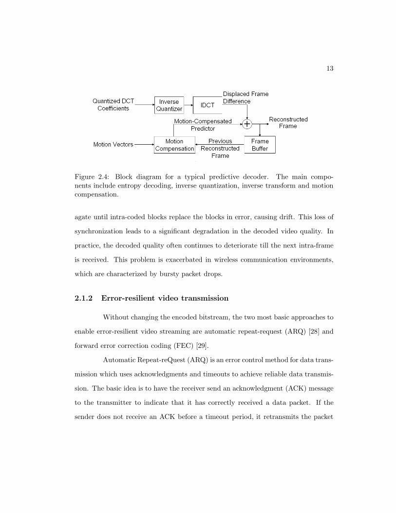
2.4 Block diagram for a typical predictive decoder. The main componentsinclude entropy decoding, inverse quantization, inverse transform andmotion compensation. . . . . . . . . . . . . . . . . . . . . . . . . . . . 13
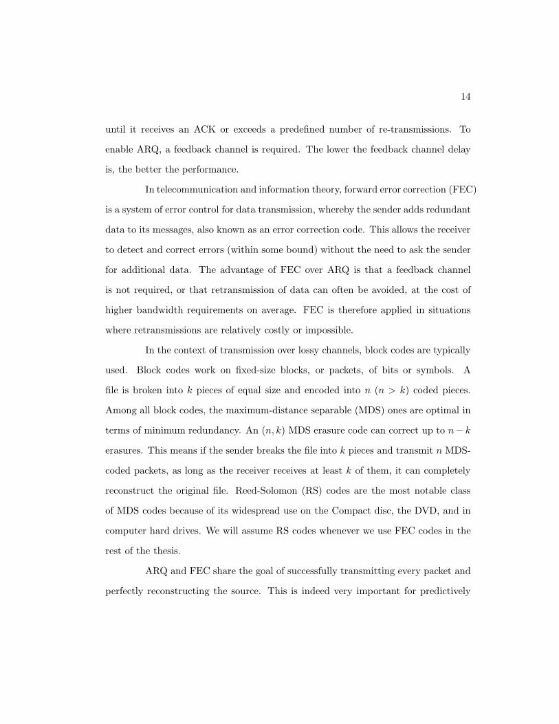
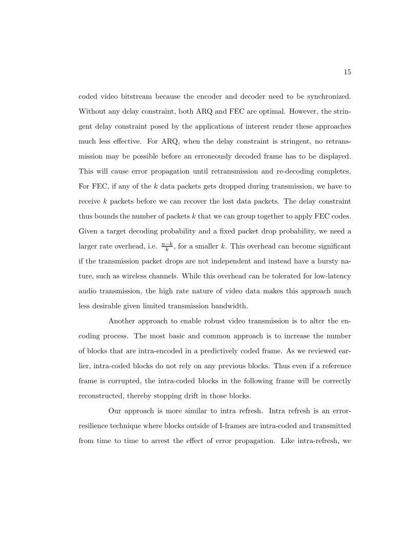
2.5 {Xi, Yi}ni=1 are i.i.d. with joint probability distribution p(x, y). Xn
is the decoder reconstruction of Xn. (a) Source Coding with Side-Information only at the decoder. (b) Source Coding with Side-Informationat both encoder and decoder. . . . . . . . . . . . . . . . . . . . . . . . 16
iv
2.6 X is a scalar real-valued number that the encoder is trying to commu-nicate to the decoder within distortion ±∆
2 . The decoder has access toside information Y . Y is a noisy version of X, and can be expressedas Y = X + N where N is the correlation noise. It is known thatX and Y are correlated such that |Y − X| < 3∆
2 . We can think ofthe quantizer as consisting of four interleaved quantizers (cosets), eachcontaining codewords whose binary labels end with the same two leastsignificant bits. The encoder, after quantizing X to X, will indicateto the decoder which one of these interleaved quantizers X belongsto. In this case, it is the quantizer in which all the codewords’ binarylabels end with “10”. The decoder can declare the closest codewordto Y in the indicated interleaved quantizer as X . . . . . . . . . . . . . 22
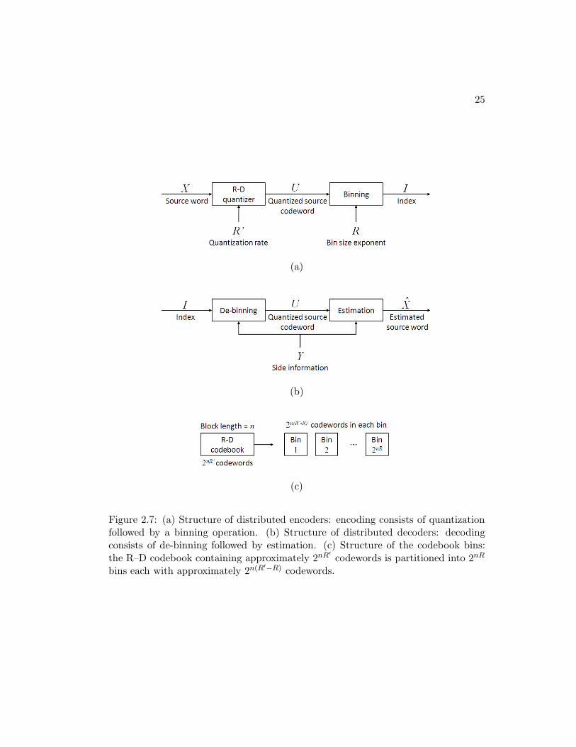
2.7 (a) Structure of distributed encoders: encoding consists of quantiza-tion followed by a binning operation. (b) Structure of distributeddecoders: decoding consists of de-binning followed by estimation. (c)Structure of the codebook bins: the R–D codebook containing ap-proximately 2nR′
codewords is partitioned into 2nR bins each withapproximately 2n(R′−R) codewords. . . . . . . . . . . . . . . . . . . . . 25
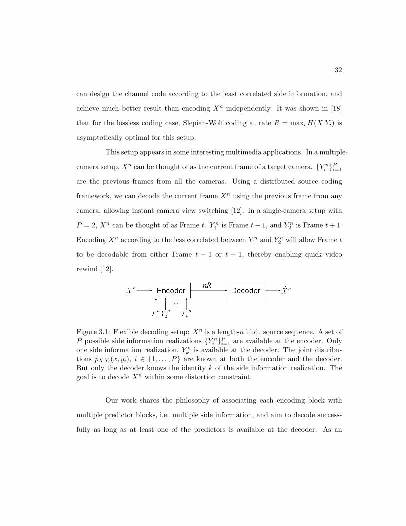
3.1 Flexible decoding setup: Xn is a length-n i.i.d. source sequence. Aset of P possible side information realizations {Y n
i }Pi=1 are available
at the encoder. Only one side information realization, Y nk is available
at the decoder. The joint distributions pX,Yi(x, yi), i ∈ {1, . . . , P} are
known at both the encoder and the decoder. But only the decoderknows the identity k of the side information realization. The goal isto decode Xn within some distortion constraint. . . . . . . . . . . . . 32
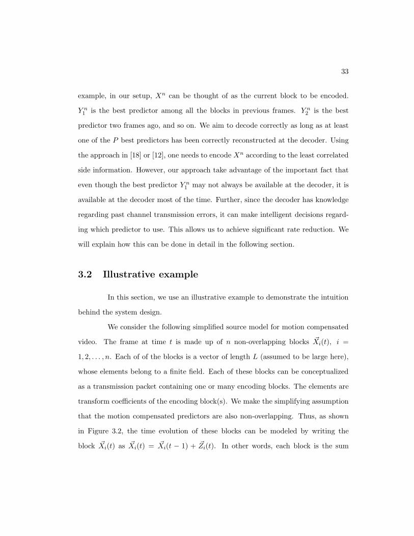
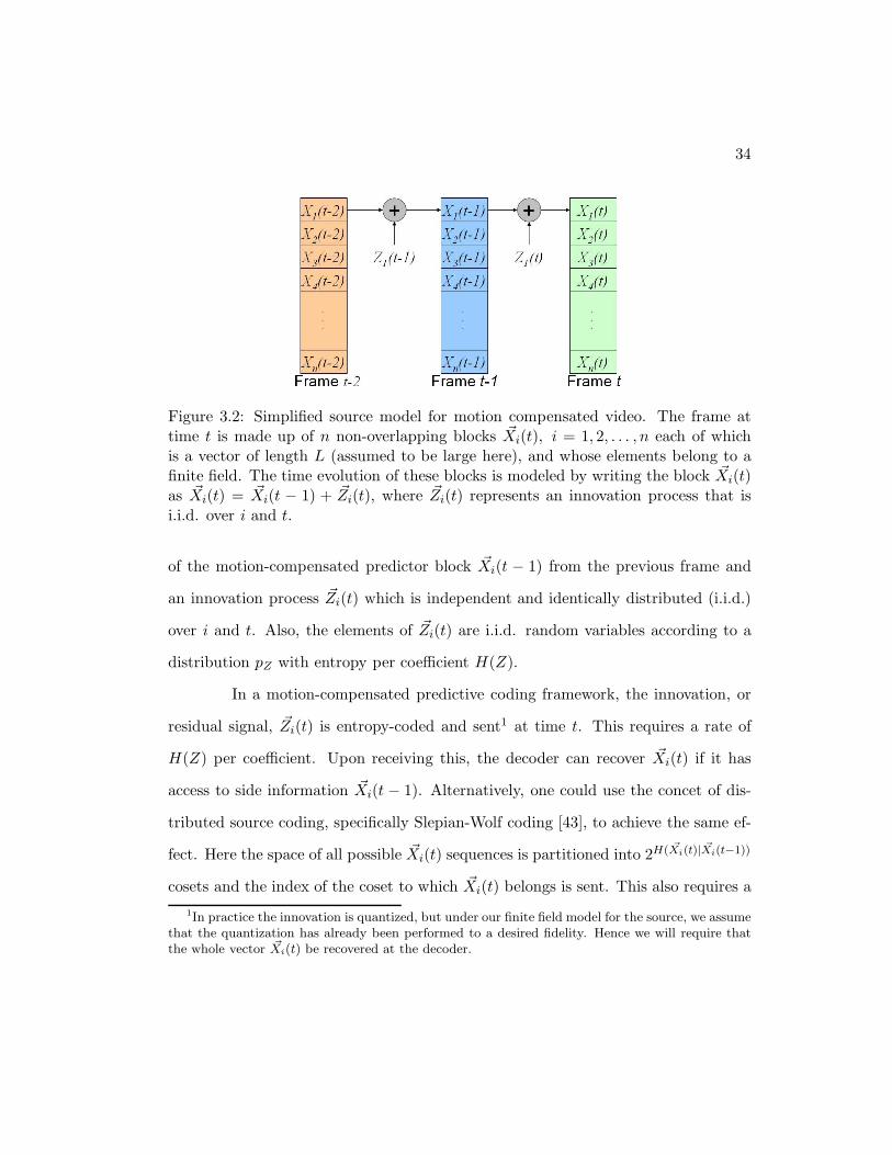
3.2 Simplified source model for motion compensated video. The frame attime t is made up of n non-overlapping blocks ~Xi(t), i = 1, 2, . . . , neach of which is a vector of length L (assumed to be large here), andwhose elements belong to a finite field. The time evolution of theseblocks is modeled by writing the block ~Xi(t) as ~Xi(t) = ~Xi(t − 1) +~Zi(t), where ~Zi(t) represents an innovation process that is i.i.d. overi and t. . . . . . . . . . . . . . . . . . . . . . . . . . . . . . . . . . . . 34
v
3.3 To represent the bursty nature of lossy wireless channels, we adopt atwo-state model to capture the effect of bursty packet drops on thevideo frames. If a frame is hit by a burst of packet drops, e.g. dueto a fade in cellular network, we say the frame is in a “bad” state.Otherwise, it is considered to be in a “good” state. The state evolvesat every time step according to a probability transition matrix. Inthe “good” state, the channel erases packets with probability pg. Inthe “bad” state, the channel erases packets with probability pb. It isassumed that pb ≫ pg. . . . . . . . . . . . . . . . . . . . . . . . . . . . 35
3.4 Finite block length analysis for the illustrative example: The plotshows the probability of the decoder failing to recover a video blockas a function of time under a typical frame state sequence. The framestate is “bad” at times t = 6, 17, 38, and “good” at other times. Weset pb = 0.3 and pg = 0.03. We assume a binary field with a Bernoulliinnovation process Z and factor p = 0.11. The number of packets ineach frame is n = 30 for practical considerations. The rate for the sub-coset information is chosen to be 26% of the rate used for the baselinecoset information. For comparison, we consider two MCPC-basedsystems with FEC: one operates at the same overall rate as the DSC-based system by using 26% extra rate for FEC, and the other uses 70%extra rate for FEC. We assume MDS codes for all systems. Under thesame latency constraint, to deliver similar performance under “good”frame state as the proposed DSC-based system, which uses 26% extrarate for sub-coset information, an MCPC-based system needs 70%extra rate for the FEC. . . . . . . . . . . . . . . . . . . . . . . . . . . 44
3.5 Block diagram for the encoder. Components in solid black lines belongto the baseline layer while components in dashed blue lines belong tothe robustness layer. . . . . . . . . . . . . . . . . . . . . . . . . . . . 45
3.6 Bit plane representation for DCT coefficients: (a) Bits marked blackare the ones that cannot be inferred from the best predictor. Bitsmarked grey are the additional ones that cannot be inferred from thesecond best predictor. (b) Bits marked in the same pattern are LDPCencoded together. . . . . . . . . . . . . . . . . . . . . . . . . . . . . . . 49
3.7 Block diagram for the decoder. Components in solid black lines belongto the baseline layer while components in dashed blue lines belong tothe robustness layer. . . . . . . . . . . . . . . . . . . . . . . . . . . . . 51
vi
3.8 Compression efficiency comparison between the baseline layer of theproposed system and H.263+ for: (a) Foreman sequence (352 × 288,1 GOP of 15 frames at 30 fps), and (b) Tempete sequence (352× 288,1 GOP of 15 frames at 30 fps). . . . . . . . . . . . . . . . . . . . . . . 54
3.9 Robustness performance of the different schemes for (a) Football (352×240, 1 GOP of 15 frames at 30 fps) and (b) Stefan (352× 240, 1 GOPof 15 frames at 30 fps) sequences using the two-state channel. In agood state, we simulate 3% independent packet drops. In a bad state,we simulate 30% independent packet drops. The bar diagram repre-sents the number of actual packet drops in each frame. For Stefan,R = 1.1mbps (15 fps), ∆R = 360kbps. For Football, R = 1.0mbps(15 fps), ∆R = 330 kbps. In (a), we also added the performance ofH.263+ baseline encoded at a higher rate. . . . . . . . . . . . . . . . . 56
3.10 Frame 3 and 4 of Football sequence using three different systems. Theproposed system has the most instant recovery from packet drops inFrame 3. . . . . . . . . . . . . . . . . . . . . . . . . . . . . . . . . . . . 58
3.11 Robustness performance of the different schemes for Football (352 ×240, 1 GOP of 15 frames at 30 fps) and Stefan (352 × 240, 1 GOPof 15 frames at 30 fps) sequences using a simulated wireless channelconforming to the CDMA 2000 1x standard. Again, for Stefan, R =1.1mbps (15 fps), ∆R = 360kbps. For Football, R = 1.0mbps (15 fps),∆R = 330 kbps. In (a), Football sequence was used and the averagepacket drop rate is 7.4%. In (b), Stefan sequence was used and theaverage packet drop rate is 7.1%. . . . . . . . . . . . . . . . . . . . . . 59
5.1 A server-based network vs. a peer-to-peer network. . . . . . . . . . . . 65
6.1 Throughput and total upload bandwidth of the system over time. Sys-tem throughput is very close to total upload bandwidth, indicatingthat leechers’, seeder’ and helpers’ upload bandwidths are all veryclose to being fully utilized. . . . . . . . . . . . . . . . . . . . . . . . . 89
6.2 Average leecher download time vs. number of pieces (k) helpers down-load. As k increases from 0, there is a drastic drop in the averageleecher download time as the helpers become able to contribute theirupload bandwidth. But as k further increases, there is a gradual in-crease in average leecher download time. This is consistent with thefluid-model analysis. . . . . . . . . . . . . . . . . . . . . . . . . . . . . 90
vii
6.3 CDF of leecher download time in three different systems. System 1:an upper-bounding setup in which helpers join the swarm with k = 8random pieces preloaded. System 2: system with regular helpers.System 3: an unaltered BitTorrent system. It shows that helpers arevery effective in reducing leechers’ average download time and theamount of resources helpers consume is negligible. . . . . . . . . . . . 91
6.4 CDF of peer download time for users with different upload/downloadbandwidths. All the leechers can benefit from helpers but the leecherswith the smallest upload bandwidth enjoy the most noticeable reduc-tion in average download time. . . . . . . . . . . . . . . . . . . . . . . 92
6.5 Proposed hybrid peer-to-peer video multicast system with helpers. . . 986.6 Average server load with different number of helpers. We also plot
the server load computed by the simple fluid-level analysis. The twocurves are fairly close, indicating that the fluid-level analysis serves asa good estimate of system performance. Server load decreases linearlyas the number of helpers increases. . . . . . . . . . . . . . . . . . . . . 109
6.7 Comparison of average server load when the peers (including helpers)are dynamic vs. when peers are static. There is only a small increasein server load when peers are dynamic. . . . . . . . . . . . . . . . . . . 110
6.8 Server load under different peer arrival rates. The average number ofpeers in the system is kept at 2000. Higher peer arrival rate implieslower peer staying time. As the peer churning rate increases, there isno significant increase in server load. . . . . . . . . . . . . . . . . . . . 111

viii
Acknowledgements
I wish to acknowledge my deep debt of gratitude to my advisor and thesis
committee chair Prof. Kannan Ramchandran for his guidance, support and encour-
agement throughout the course of my graduate study. This research would not have
been possible without his vision and motivation.
I am extremely grateful to the other members of my dissertation committee
Professor Zakhor and Professor Olshausen who also served on my qualifying exam
committee for their invaluable feedback on this dissertation. I would like to thank my
colleagues Abhik Majumdar, Vinod Prabhakaran, Alex Dimakis, and Chuohao Yeo
for their invaluable help at various stages of my research and for the many productive
discussions that we had. I would also like to thank everyone from the Collaboration
and Communication Systems group at Microsoft Research, especially Minghua Chen,
Cheng Huang and Jin Li, for a fulfilling research experience.
I would like to thank all my friends at Berkeley and all the members of
the BASiCS group and Wireless Foundations for making my stay at Berkeley a
memorable and enjoyable one.
My parents have been a constant source of encouragement without whose
love and support I would not have been able to make it this far. I am deeply indebted
to them.

1
Chapter 1
Introduction
With the explosive development of communication networks, demand for
multimedia applications has grown not only in quantity but also in variety and
quality. Consumers are no longer content to watching TV over cable networks or
DVDs from Blockbuster. Now there is demand to download and watch high definition
movies over the Internet, watch live sports broadcast using our laptops, have a video
conference using our cell phones, and watch high-quality videos on YouTube. In this
dissertation, we focus on two important classes of video applications.
In Part I, we consider the problem of low-latency video streaming over
packet networks characterized by bursty losses, such as wireless networks. In partic-
ular, we focus on applications characterized by stringent end-to-end delay constraints
that are of the order of a fraction of a second.1 Examples include video telephony, in-
teractive distance learning, and video surveillance. Compared to traditional wireline
networks, today’s dominant transmission channels, such as WiFi and cellular net-
1A necessary requirement for conversational services is for end-to-end delay to be less than 250milliseconds[44].
2
works, are prone to transmission errors. As a result, in addition to the conventional
requirement of high compression efficiency, such applications require the compressed
bitstream to be robust to packet losses caused by transmission errors. These require-
ments need to be met simultaneously and under stringent delay constraints.
While today’s popular video coders, such as MPEG-x and H.26x [25, 15,
9, 10, 48], can compress video signals efficiently, the compressed bitstream is sus-
ceptible to packet losses. This is a direct consequence of the motion-compensated
predictive coding (MCPC) framework that underlies these codecs. Conventional ap-
proaches, such as automatic repeat-request (ARQ) [28] and forward error correction
codes (FEC) [29], focus on ensuring that the decoder receive the entire compressed
bitstream, either through retransmission or error-correcting decoding. These are
very effective techniques for scenarios involving independent packet losses and more
lenient end-to-end delay constraints. However, wireless transmission media are char-
acterized by bursty packet drops. This unique attribute makes low-latency streaming
applications highly challenging.
We take an alternative approach and present a video coding framework
based on information theoretical principles of distributed source coding (DSC) [43,
50]. Instead of guaranteeing delivery of every data packet, the proposed codec allows
occasional frame corruptions due to bursty packet drops. Instead, it arrests the effect
of such frame corruptions immediately in the following frames, thus maintaining high
visual quality. We summarize our contributions in this part of this thesis as follows.
• On the theoretical side, we illustrate the proposed method through a simple but
conceptually illustrative model. This analytically tractable model captures the
essence of the dynamics related to transmitting temporally dependent source
3
information over packet erasure channels. Under certain modeling assump-
tions, we quantify the performance gains of the proposed distributed source
coding based video codec over a conventional predictive coding system, such
as MPEGx/H.26x, when the video stream is transmitted over a lossy channel.
• Building on the insights from the theoretical model, we implement a practical
video coding system. We present extensive simulation results, which demon-
strate the strengths and weaknesses of the proposed system over standard ap-
proaches, such as protecting predictively coded bitstream with FEC codes and
random intra refresh.
In Part II, we focus on video distribution over peer-to-peer (P2P) networks.
Video distribution over Internet using the traditional client-server method places
tremendous burden on existing infrastructure, such as data centers and content dis-
tribution networks (CDN). In fact, the existing client-server infrastructure lacks the
scalability to support an increasingly large user base due to limited backbone ca-
pacity [5]. P2P-based Internet video distribution, both download and streaming
applications, can greatly reduce server bandwidth costs of content providers and by-
pass bottlenecks between providers and consumers. In a P2P content distribution
network, peers interested in the same content form an overlay network. The content
of interest is broken into pieces. Peers upload and download these pieces simul-
taneously among themselves thus offloading server burden by utilizing the upload
bandwidth of participating peers.
There are many aspects to improving a P2P network. In Chapter 6 of the
dissertation, we focus on easing the bottleneck of P2P network performance caused
by the asymmetry of today’s Internet connections. Specifically, we study how to
4
improve the performance of P2P networks for video download and multicast through
a higher level of collaboration among peers. The system throughput of a P2P network
is capped by the smaller one between the total system upload bandwidth and the
total system download bandwidth [38]. However, a large population of Internet users
today have highly asymmetric Internet connections, such as ADSL and cable, and
have much lower upload than download bandwidth. As a result, peers’ total available
upload capacity often becomes the most dominant constraint of a P2P network.
We propose to overcome this constraint by promoting a higher level of
collaboration among network peers to optimize performance of uplink-scarce collab-
orative networks beyond what can be achieved by conventional P2P networks. One
important observation is that at any given time, while there are peers exhausting
their upload bandwidth sharing data, there are also numerous peers with spare up-
load capacity. This is a direct result of the statistical multiplexing property of a
large-scale system in the sense that peers have not only different physical capabili-
ties but also different behavioral characteristics. We call such peers helpers. Helpers
represent a rich untapped resource, whose upload bandwidth can be exploited to
increase the total system upload bandwidth and hence ease the performance bottle-
neck. We study the efficient use of helpers for P2P video download and extend the
philosophy to live video multicast. We make the following contributions.
• For video download, we use average peer download time as the performance
metric and develop a distributed helper protocol that is backwards-compatible
with the popular BitTorrent file sharing protocol [14]. We analyze steady-state
system performance using a modified version of the fluid model of Qiu and
Srikant [38], and also make corrections to the analysis presented there. We
5
demonstrate both analytically and empirically that helpers’ upload bandwidth
can be efficiently utilized using the proposed protocol and verify the accuracy
of the fluid model analysis.
• For live multicast, we aim to minimize server load of a P2P live multicast sys-
tem in which peers’ average upload bandwidth is smaller than video bitrate.
We use a simple first-order analysis to derive the performance upper bound and
use it to guide the design of a constructive solution. We show through exten-
sive simulation that the proposed strategy can closely match this performance
bound.
6
Part I
Robust video transmission over
lossy networks

7
Chapter 2
Motivation and background
Real-time video transmission over lossy networks is an area that has been
widely studied by both academia and industry. Two of the main reasons are:
• Today’s popular transmission media, such as the Internet and cellular networks,
are prone to transmission packet losses;
• Though today’s popular video coders, such as MPEG-x and H.26x [25, 15, 9,
10, 48], can compress videos efficiently, the compressed bitstream is susceptible
to packet losses.
The fragility of MPEG-like compressed bitstream is a direct consequence of
the predictive coding framework that underlies these codecs. At a high level, each
frame of the video is divided into non-overlapping blocks. Each encoding block is
“matched” with the most similar block in the previous frame, called predictor block.
Only the difference between the two blocks is encoded. In other words, each block is
deterministically associated with one single predictor. If that predictor is corrupted
8
due to channel loss, there will be a predictor mismatch between encoder and decoder.
When this happens, even if the difference between the current block and the predictor
block is correctly received, the reconstruction will still be erroneous. This error will
propagate until the next independently encoded frame is decoded, causing severe
visual quality degradation.
A number of novel ideas and useful tools have been developed to enable
robust transmission of predictively encoded video bitstreams, including automatic
repeat request (ARQ) [28], forward error correction codes (FEC) [29], and a com-
bination of the two (hybrid ARQ), etc. These techniques focus on ensuring that
the decoder receive the entire compressed bitstream. They are very effective with
independent packet drops and more lenient constraints on end-to-end delay.
We focus on a class of applications with stringent end-to-end delay con-
straints that are of the order of a fraction of a second. Examples include video tele-
phony, interactive distance learning, and video surveillance. Further, wireless trans-
mission media are characterized by bursty packet drops. These unique characteristics
make the problem especially challenging, compared to regular video-streaming ap-
plications, which can allow up to tens of seconds of buffering.
We propose to take an alternative approach and present a video coding
framework based on information theoretical principles of distributed source coding
(DSC) [43, 50]. Instead of trying to recover every data packet, the proposed codec
allows frames transmitted under poor channel condition to be corrupted, but arrests
the effect of packet drops immediately in the following frames. Specifically, we aim
to recover a block even if the predictor block at the decoder is corrupted and cannot
be predicted at the encoder. This is possible because in the DSC framework, each
9
encoding block is no longer encoded based on a single predictor in a deterministic
fashion, e.g. via differential coding. Instead, each block is encoded based on the
statistical correlation between the block and the best predictor available at the de-
coder using channel coding techniques. Once a block is channel coded targeting a
specific correlation, any predictor at the decoder that is sufficiently correlated with
the current block can be used to decode the block correctly. Using the terminology
of information theory, the current block to be encoded is called the source, and the
candidate predictor used for decoding is called the side information.
There are two important aspects of using distributed source coding frame-
work. First, the decoder needs to have a high-quality side information. Second, the
encoder needs to be able to accurately estimate the correlation between the cur-
rent block and the side information. In the scenario of video streaming over lossy
channel, as video data is highly non-stationary, correlation estimation in the pres-
ence of unpredictable channel noise remains a challenging open question in general.
In this work, we propose a video coding system that carries out a joint side infor-
mation selection and correlation estimation scheme. By doing this and following a
joint source-channel coding approach, the proposed DSC-based codec can efficiently
tune to both the source content as well as to the network loss characteristics while
respecting stringent latency constraints.
10
2.1 Video coding and distributed source coding back-
ground
We review background knowledge on both the predictive video coding archi-
tecture and principles of distributed source coding so that we can better understand
the fragility of predictively encoded video bitstreams in the face of transmission errors
and the theoretical foundation underlying the proposed system.
2.1.1 Predictve video coding background
First, we present a quick overview of the conventional motion-compensated
predictive video coding architecture that underlies current video coding standards
such as the MPEG-x and H.26x standards.
A video sequence is a collection of images (also called pictures, frames)
in time. Uncompressed video data contain both spatial and temporal redundancy.
Spatial redundancy can be reduced through applying Discrete Cosine Transform
(DCT) to the images while temporal redundancy is typically reduced through motion
compensation. For the purpose of encoding, each of these frames is decomposed into
a grid of non-overlapping blocks. These blocks are encoded primarily in the following
two modes to exploit spatial and/or temporal redundancy.
1. Intra-Coding (I) Mode: The intra-coding mode exploits only the spatial
correlation in the frame by using the Discrete Cosine Transform (DCT) to
each block that is intra-coded. It typically has poor compression efficiency,
since it does not exploit the temporal redundancy in a video sequence.
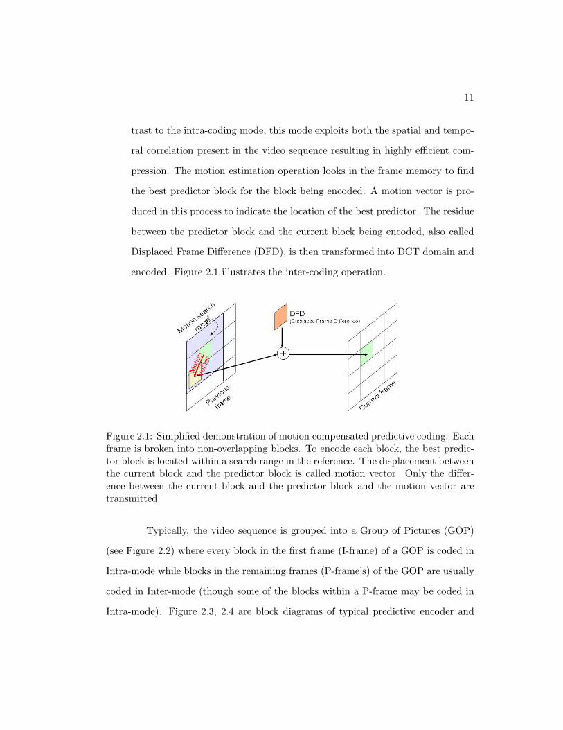
2. Inter-Coding or Motion Compensated Predictive (P) Mode: In con-
11
trast to the intra-coding mode, this mode exploits both the spatial and tempo-
ral correlation present in the video sequence resulting in highly efficient com-
pression. The motion estimation operation looks in the frame memory to find
the best predictor block for the block being encoded. A motion vector is pro-
duced in this process to indicate the location of the best predictor. The residue
between the predictor block and the current block being encoded, also called
Displaced Frame Difference (DFD), is then transformed into DCT domain and
encoded. Figure 2.1 illustrates the inter-coding operation.
Figure 2.1: Simplified demonstration of motion compensated predictive coding. Eachframe is broken into non-overlapping blocks. To encode each block, the best predic-tor block is located within a search range in the reference. The displacement betweenthe current block and the predictor block is called motion vector. Only the differ-ence between the current block and the predictor block and the motion vector aretransmitted.
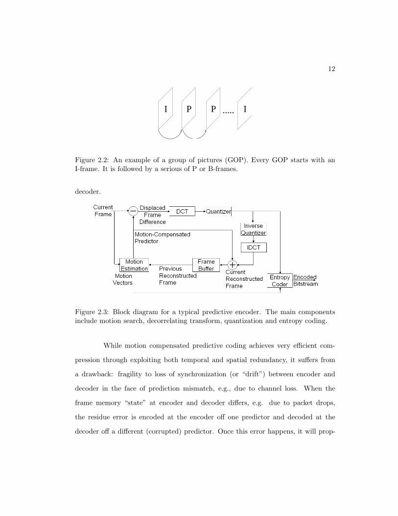
Typically, the video sequence is grouped into a Group of Pictures (GOP)
(see Figure 2.2) where every block in the first frame (I-frame) of a GOP is coded in
Intra-mode while blocks in the remaining frames (P-frame’s) of the GOP are usually
coded in Inter-mode (though some of the blocks within a P-frame may be coded in
Intra-mode). Figure 2.3, 2.4 are block diagrams of typical predictive encoder and
12
I.....PPI
Figure 2.2: An example of a group of pictures (GOP). Every GOP starts with anI-frame. It is followed by a serious of P or B-frames.
decoder.
Figure 2.3: Block diagram for a typical predictive encoder. The main componentsinclude motion search, decorrelating transform, quantization and entropy coding.
While motion compensated predictive coding achieves very efficient com-
pression through exploiting both temporal and spatial redundancy, it suffers from
a drawback: fragility to loss of synchronization (or “drift”) between encoder and
decoder in the face of prediction mismatch, e.g., due to channel loss. When the
frame memory “state” at encoder and decoder differs, e.g. due to packet drops,
the residue error is encoded at the encoder off one predictor and decoded at the
decoder off a different (corrupted) predictor. Once this error happens, it will prop-
13
Figure 2.4: Block diagram for a typical predictive decoder. The main compo-nents include entropy decoding, inverse quantization, inverse transform and motioncompensation.
agate until intra-coded blocks replace the blocks in error, causing drift. This loss of
synchronization leads to a significant degradation in the decoded video quality. In
practice, the decoded quality often continues to deteriorate till the next intra-frame
is received. This problem is exacerbated in wireless communication environments,
which are characterized by bursty packet drops.
2.1.2 Error-resilient video transmission
Without changing the encoded bitstream, the two most basic approaches to
enable error-resilient video streaming are automatic repeat-request (ARQ) [28] and
forward error correction coding (FEC) [29].
Automatic Repeat-reQuest (ARQ) is an error control method for data trans-
mission which uses acknowledgments and timeouts to achieve reliable data transmis-
sion. The basic idea is to have the receiver send an acknowledgment (ACK) message
to the transmitter to indicate that it has correctly received a data packet. If the
sender does not receive an ACK before a timeout period, it retransmits the packet
14
until it receives an ACK or exceeds a predefined number of re-transmissions. To
enable ARQ, a feedback channel is required. The lower the feedback channel delay
is, the better the performance.
In telecommunication and information theory, forward error correction (FEC)
is a system of error control for data transmission, whereby the sender adds redundant
data to its messages, also known as an error correction code. This allows the receiver
to detect and correct errors (within some bound) without the need to ask the sender
for additional data. The advantage of FEC over ARQ is that a feedback channel
is not required, or that retransmission of data can often be avoided, at the cost of
higher bandwidth requirements on average. FEC is therefore applied in situations
where retransmissions are relatively costly or impossible.
In the context of transmission over lossy channels, block codes are typically
used. Block codes work on fixed-size blocks, or packets, of bits or symbols. A
file is broken into k pieces of equal size and encoded into n (n > k) coded pieces.
Among all block codes, the maximum-distance separable (MDS) ones are optimal in
terms of minimum redundancy. An (n, k) MDS erasure code can correct up to n− k
erasures. This means if the sender breaks the file into k pieces and transmit n MDS-
coded packets, as long as the receiver receives at least k of them, it can completely
reconstruct the original file. Reed-Solomon (RS) codes are the most notable class
of MDS codes because of its widespread use on the Compact disc, the DVD, and in
computer hard drives. We will assume RS codes whenever we use FEC codes in the
rest of the thesis.
ARQ and FEC share the goal of successfully transmitting every packet and
perfectly reconstructing the source. This is indeed very important for predictively
15
coded video bitstream because the encoder and decoder need to be synchronized.
Without any delay constraint, both ARQ and FEC are optimal. However, the strin-
gent delay constraint posed by the applications of interest render these approaches
much less effective. For ARQ, when the delay constraint is stringent, no retrans-
mission may be possible before an erroneously decoded frame has to be displayed.
This will cause error propagation until retransmission and re-decoding completes.
For FEC, if any of the k data packets gets dropped during transmission, we have to
receive k packets before we can recover the lost data packets. The delay constraint
thus bounds the number of packets k that we can group together to apply FEC codes.
Given a target decoding probability and a fixed packet drop probability, we need a
larger rate overhead, i.e. n−kk
, for a smaller k. This overhead can become significant
if the transmission packet drops are not independent and instead have a bursty na-
ture, such as wireless channels. While this overhead can be tolerated for low-latency
audio transmission, the high rate nature of video data makes this approach much
less desirable given limited transmission bandwidth.
Another approach to enable robust video transmission is to alter the en-
coding process. The most basic and common approach is to increase the number
of blocks that are intra-encoded in a predictively coded frame. As we reviewed ear-
lier, intra-coded blocks do not rely on any previous blocks. Thus even if a reference
frame is corrupted, the intra-coded blocks in the following frame will be correctly
reconstructed, thereby stopping drift in those blocks.
Our approach is more similar to intra refresh. Intra refresh is an error-
resilience technique where blocks outside of I-frames are intra-coded and transmitted
from time to time to arrest the effect of error propagation. Like intra-refresh, we
16
also do not attempt to recover every dropped packet. Instead, we aim to arrest the
effect of packet drops immediately after. However, the proposed scheme is much
more compression-efficient in that it makes use of the temporal correlation between
the current block and predictors in possibly corrupted erroneous frames.
The following section provides an overview of a particular setup of dis-
tributed source coding that is of interest: source coding with side-information. The
key concepts will be illustrated through examples to provide intuition on why the
framework of distributed source coding is potentially beneficial for transmission with
losses.
2.1.3 Distributed source coding background
(a)
(b)
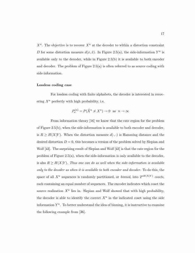
Figure 2.5: {Xi, Yi}ni=1 are i.i.d. with joint probability distribution p(x, y). Xn is
the decoder reconstruction of Xn. (a) Source Coding with Side-Information only atthe decoder. (b) Source Coding with Side-Information at both encoder and decoder.
Consider the problems depicted in Figures 2.5(a) and (b). {Xi, Yi}ni=1 are
i.i.d. with joint probability distribution p(x, y). Xn is the decoder reconstruction of
17
Xn. The objective is to recover Xn at the decoder to within a distortion constraint
D for some distortion measure d(x, x). In Figure 2.5(a), the side-information Y n is
available only to the decoder, while in Figure 2.5(b) it is available to both encoder
and decoder. The problem of Figure 2.5(a) is often referred to as source coding with
side-information.
Lossless coding case
For lossless coding with finite alphabets, the decoder is interested in recov-
ering Xn perfectly with high probability, i.e.
P (n)e = P (Xn 6= Xn) → 0 as n → ∞
From information theory [16] we know that the rate region for the problem
of Figure 2.5(b), when the side-information is available to both encoder and decoder,
is R ≥ H(X|Y ). When the distortion measure d(·, ·) is Hamming distance and the
desired distortion D = 0, this becomes a version of the problem solved by Slepian and
Wolf [43]. The surprising result of Slepian and Wolf [43] is that the rate region for the
problem of Figure 2.5(a), when the side-information is only available to the decoder,
is also R ≥ H(X|Y ). Thus one can do as well when the side-information is available
only to the decoder as when it is available to both encoder and decoder. To do this, the
space of all Xn sequences is randomly partitioned, or binned, into 2nH(X|Y ) cosets,
each containing an equal number of sequences. The encoder indicates which coset the
source realization Xn lies in. Slepian and Wolf showed that with high probability,
the decoder is able to identify the correct Xn in the indicated coset using the side
information Y n. To better understand the idea of binning, it is instructive to examine
the following example from [36].
18
Illustrative Example for Slepian-Wolf Coding: Let X and Y be length 3-bit
binary data that can equally likely take on each of the 8 possible values. X and Y
are correlated such that the Hamming distance between them is at most 1. That is,
given Y (e.g., [0 1 0]), X is either the same as Y ([0 1 0]) or differs in one of the
three bits ([1 1 0], [0 0 0] or [0 1 1]). The goal is to efficiently encode X in the two
scenarios depicted in Figures 2.5(a) and (b) so that it can be perfectly reconstructed
at the decoder. Information theory prescribes that we cannot hope to compress X
to fewer than 2 bits as H(X|Y ) = 2. We will now explain how this can be achieved
in both of the scenarios in Figure 2.5.
Scenario 1: In the first scenario (see Figure 2.5(b)), Y is present both at
the encoder and at the decoder. The encoder can simply calculate the residue X⊕Y
and send the information. Since there are only four possible values of X ⊕Y ([0 0 0],
[0 0 1], [0 1 0] and [1 0 0]), the encoder only needs to send 2 bits to signal the value.
The decoder will then recover X through X ⊕Y ⊕Y . In the context of video coding,
X is analogous to the current video block that is being encoded, Y is analogous to
the motion-compensated predictor from the frame memory, the residue between X
and Y is analogous to the displaced frame difference, hence this mode of encoding is
similar to predictive coding.
Scenario 2: In this setup, Y is made available only to the decoder (see
Figure 2.5(a)). The encoder for X does not have access to Y but it does know the
correlation structure between X and Y and also the fact that the decoder has access
to Y . Since this scenario is strictly not better than the first scenario, its performance
is limited by that of the first scenario. However, from the Slepian-Wolf theorem [43]
we know that even in this seemingly worse case, we can achieve the same performance
19
as in the first scenario (i.e. encode X using 2 bits).
This can be done using the following approach. The space of possible values
(codewords) of X is partitioned into 4 sets (called cosets) each containing 2 code-
words, namely, Coset 1 ([0 0 0] and [1 1 1]), Coset 2 ([0 0 1] and [1 1 0]), Coset 3
([0 1 0] and [1 0 1]) and Coset 4 ([1 0 0] and [0 1 1]). The encoder for X identifies
the coset containing the codeword for X and sends the index for the coset in 2 bits
instead of the actual codeword. The decoder, in turn, upon receiving the coset index,
uses Y to disambiguate the correct X from the set by declaring the codeword that
is closest to Y as the answer. Note that this is feasible because the distance between
X and Y is at most 1, while the distance between the two codewords in any set is 3.
We note that Coset 1 in the above example is a repetition channel code [29]
of distance 3 and the other sets are cosets [19, 20] of this code in the codeword space
of X. In channel coding terminology, each coset is associated with an unique index,
called syndrome. We have used a channel code that is “matched” to the correlation
distance (or equivalently, noise) between X and Y to partition the source codeword
space of X (which is the set of all possible 3 bit words) into cosets of the 3-bit
repetition channel code. The decoder here needs to perform channel decoding since
it needs to identify the source codeword from the list of codewords enumerated in the
coset indicated by the encoder. To do so, it finds the codeword in the signalled coset
that is closest to Y . Since the encoder sends the index or syndrome for the coset
containing the codeword for X to the decoder, we sometimes refer to this operation
as syndrome coding.
We now compare Scenario 1 and 2 and demonstrate the inherent robustness
of the distributed source coding framework. Let Y be [0 0 0] and X be [0 0 1]. Under
20
Scenario 1, we use two bits to indicate to the decoder that X⊕Y = [010]. If for some
reason Y at decoder gets corrupted and becomes [0 0 1], the decoder will decode X
to be [0 0 1] ⊕ [0 1 0] = [0 1 1], which is incorrect. Under Scenario 2, on the other
hand, we use two bits to indicate that X belones to Coset 2 ([0 0 1] and [1 1 0]).
Now, if Y becomes [0 0 1] accidentally, the decoder will still decode X to be [0 0 1] as
this is the codeword closest to the side information Y under Hamming distortion. In
fact, if as long as Y remains within Hamming distance 1 to X, decoding will always
succeed.
We now turn to the case when we are interested in recovering Xn at the
decoder to within some distortion.
Lossy coding case
Consider again the problem of Figure 2.5(a). We now remove the constraint
on X and Y to be discrete and allow them to be continuous random variables as
well. We are now interested in recovering Xn at the decoder to within a distortion
constraint D for some distortion measure d(x, x). Let {Xi, Yi}ni=1 be i.i.d. with
joint probability distribution p(x, y) and let the distortion measure be d(xn, xn) =
1n
∑ni=1 d(xi, xi). Then the Wyner-Ziv theorem [50] states that the rate distortion
function for this problem is
R(D) = minp(u|x)p(x|u,y)
I(X;U) − I(Y ;U)
where
p(x, y, u) = p(u|x)p(x, y)
21
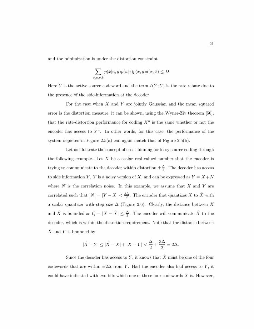
and the minimization is under the distortion constraint
∑
x,u,y,x
p(x|u, y)p(u|x)p(x, y)d(x, x) ≤ D
Here U is the active source codeword and the term I(Y ;U) is the rate rebate due to
the presence of the side-information at the decoder.
For the case when X and Y are jointly Gaussian and the mean squared
error is the distortion measure, it can be shown, using the Wyner-Ziv theorem [50],
that the rate-distortion performance for coding Xn is the same whether or not the
encoder has access to Y n. In other words, for this case, the performance of the
system depicted in Figure 2.5(a) can again match that of Figure 2.5(b).
Let us illustrate the concept of coset binning for lossy source coding through
the following example. Let X be a scalar real-valued number that the encoder is
trying to communicate to the decoder within distortion ±∆2 . The decoder has access
to side information Y . Y is a noisy version of X, and can be expressed as Y = X +N
where N is the correlation noise. In this example, we assume that X and Y are
correlated such that |N | = |Y − X| < 3∆2 . The encoder first quantizes X to X with
a scalar quantizer with step size ∆ (Figure 2.6). Clearly, the distance between X
and X is bounded as Q = |X − X | ≤ ∆2 . The encoder will communicate X to the
decoder, which is within the distortion requirement. Note that the distance between
X and Y is bounded by
|X − Y | ≤ |X − X| + |X − Y | <∆
2+
3∆
2= 2∆.
Since the decoder has access to Y , it knows that X must be one of the four
codewords that are within ±2∆ from Y . Had the encoder also had access to Y , it
could have indicated with two bits which one of these four codewords X is. However,
22
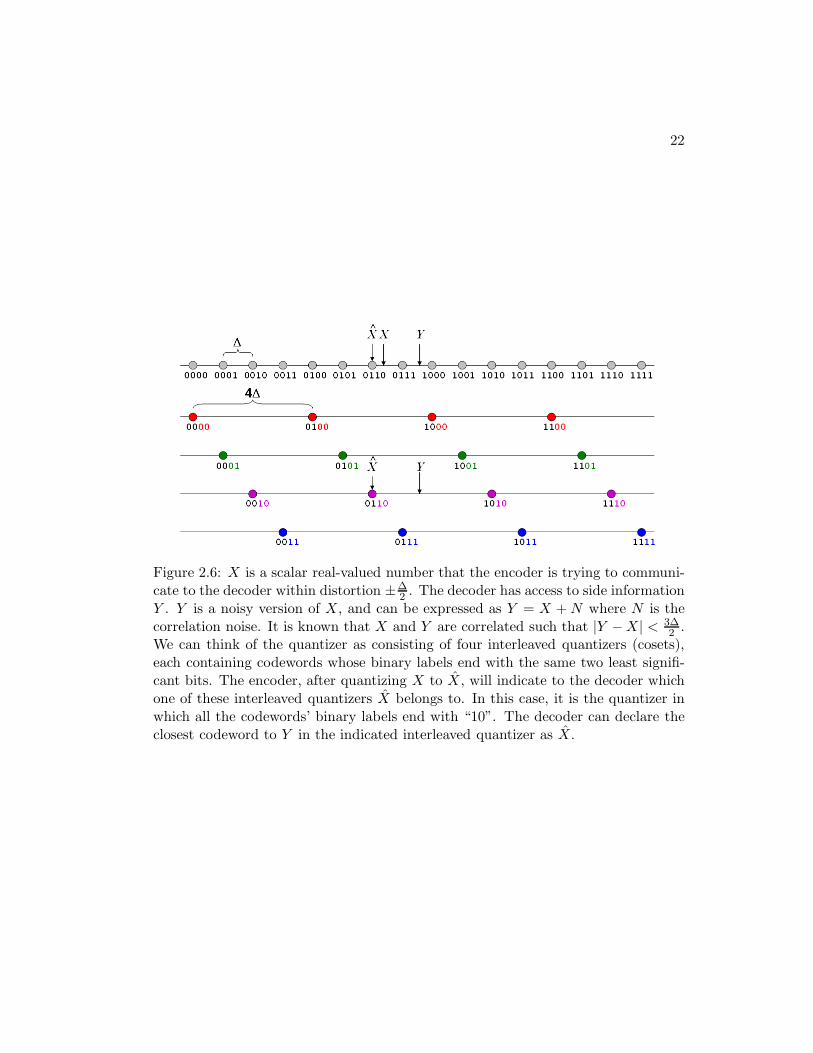
Figure 2.6: X is a scalar real-valued number that the encoder is trying to communi-cate to the decoder within distortion ±∆
2 . The decoder has access to side informationY . Y is a noisy version of X, and can be expressed as Y = X + N where N is thecorrelation noise. It is known that X and Y are correlated such that |Y − X| < 3∆
2 .We can think of the quantizer as consisting of four interleaved quantizers (cosets),each containing codewords whose binary labels end with the same two least signifi-cant bits. The encoder, after quantizing X to X , will indicate to the decoder whichone of these interleaved quantizers X belongs to. In this case, it is the quantizer inwhich all the codewords’ binary labels end with “10”. The decoder can declare theclosest codeword to Y in the indicated interleaved quantizer as X.
23
even when the encoder does not have access to Y , it is possible to communicate
X to the decoder using only two bits. To see this, we can think of the quantizer
(codebook) as consisting of four interleaved quantizers (cosets), each of step size 4∆,
as shown in Figure 2.6. The encoder, after quantizing X to X , can indicate to the
decoder which one of these interleaved quantizers (coset) X belongs to, which also
requires two bits. Since the step size of each of the four interleaved quantizers is
4∆, each of them has exactly one of the four codewords that are within ±2∆ from
Y . Therefore, the decoder can declare the closest codeword to Y in the indicated
interleaved quantizer as X.
In assigning a unique two-bit symbol, or syndrome, to each interleaved
quantizer (coset), we see that each of them contains codewords whose binary labels
share the same two least significant bits. For example, the labels of the codewords in
the first coset all end with bits “00”. Therefore a natural way to indicate a coset is to
use the common least significant bits. The number of least significant bits needed to
indicate a coset depends on how many cosets the codebook is broken into, which in
turn depends on the statistics of the correlation noise N . We adopt this multi-level
coding scheme [45] in our implementation.
Like in the lossless coding example, even if Y at the decoder becomes cor-
rupted, as long as it does not violate the correlation constraint, i.e. as long as
Y − X < 2∆, decoding will succeed. In general, the fact that the encoder is able
to compress the source Xn using only the statistical correlation between Xn and
Y n, without having access to a deterministic copy of the side-information Y n, is the
reason for the inherent robustness of the distributed source coding framework and
makes it a promising framework to enables robust video transmission.
24
Let us now take a more formal look at Wyner-Ziv encoding and decoding.
Wyner-Ziv encoding and decoding: As in regular source coding, encoding pro-
ceeds by first designing a rate-distortion codebook of rate R′ (containing 2nR′
code-
words) constituting the space of quantized codewords for X. Each n-length block
of source samples X is first quantized to the “nearest” codeword in the codebook.
As in the illustrative example above, the quantized codeword space (of size 2nR′
codewords) is further partitioned into 2nR cosets or bins (R < R′) so that each bin
contains 2n(R′−R) codewords. This can be achieved by the information theoretic op-
eration of random binning. The encoder transmits only the index of the bin in which
the quantized codeword lies and thereby only needs R bits/sample.
The decoder receives the bin index and disambiguates the correct codeword
in this bin by exploiting the correlation between the codeword and the matching
n-length block of side-information samples Y. This operation is akin to channel
decoding. Once the decoder recovers the codeword, if MSE is the distortion measure,
it forms the minimum MSE estimate of the source to achieve an MSE of D.
An important feature of the coset binning method that we exploit is the
fact that if the side information at the decoder is inferior to what the DSC code was
designed for, the decoder can still make use of this transmission if a small amount
of additional information is made available. Continuing the example above, suppose
that after the transmission, the encoder finds out that the actual side information
Y ′ available at the decoder is of an inferior quality |Y ′ − X| < 7∆2 . All the encoder
needs to do is to further partition each of the four interleaved quantizers into two
sub-quantizers and indicate to the decoder which sub-quantizer X belongs to using
one additional bit. Together with the two bit originally received, the decoder can
25
(a)
(b)
(c)
Figure 2.7: (a) Structure of distributed encoders: encoding consists of quantizationfollowed by a binning operation. (b) Structure of distributed decoders: decodingconsists of de-binning followed by estimation. (c) Structure of the codebook bins:the R–D codebook containing approximately 2nR′
codewords is partitioned into 2nR
bins each with approximately 2n(R′−R) codewords.
26
now correctly decode X given the inferior side information Y ′. It is important to
note that the two bits sent in the first transmission are entirely useful even given
the inferior side information. This feature is unique to the DSC framework, which
allows us to take a layered approach and separate the baseline layer and robustness
layer without losing any compression efficiency. This separation will further enable
compression of the robustness layer as we will later demonstrate.
From distributed source coding principles to video coding
There are two major assumptions in the classical distributed source coding
setup. First, the decoder has one and only one side information to use. Second,
both the encoder and decoder know the correlation between the source and the side
information. These assumptions are unfortunately not true for practical video coding.
First, video data is highly redundant both spatially and temporally. For each block,
there are a lot of correlated previously decoded blocks available at the decoder that
can be used as the side information. When there are transmission packet drops, it
becomes unclear which previously decoded block is the most correlated to the current
block. Second, neither the encoder nor the decoder has knowledge of the correlation
between the source and side information because video data is highly non-stationary.
Even though the encoder can learn the correlation through motion search, in the
presence of packet drops that the encoder cannot anticipate, correlation estimation
becomes very challenging.
These differences between theory and practice dictates that there are two
important aspect to video coding using distributed principles. First, the decoder
needs to use a high-quality side information. If the decoder picks a side information
27
that is poorly correlated to the source, the encoding rate will be higher than necessary
to ensure successful decoding, thus losing compression efficiency. Second, the encoder
needs to be able to accurately estimate the correlation between the current block and
the side information. If we underestimate the correlation between the current block
and the best predictor block at the decoder, we will use a channel code that is
stronger than necessary, hence losing compression efficiency. On the other hand,
if we overestimate the correlation, channel decoding will fail, causing video quality
degradation.
In the following chapter, we will illustrate through a simple illustrative ex-
ample how the proposed system addresses these two issues simultaneously by making
use of channel characteristics and decoder’s knowledge regarding past packet drop
patterns.
28
Chapter 3
Distributed source coding based
robust video transmission over
networks with bursty losses
3.1 Related work
There have been a number of novel and interesting works that use dis-
tributed source coding to tackle various challenges in video coding and transmission.
The challenges include but are not limited to low-complexity video encoding (e.g. [21,
37, 7] and the references within), robust video transmission (e.g. [37, 40, 21, 27]),
scalable video coding (e.g. [51, 46]), and multi-view video coding (e.g. [23] and the
references within). In this section, we focus on reviewing related works on robust
video transmission using DSC [37, 40, 21, 47, 27], and flexible video decoding using
DSC [12].
29
3.1.1 Robust video transmission using distributed source coding
In the example in Section 2.1.3, we note that as long as the side information
Y remains within ±3∆2 of X, the decoder will always correctly decode X . This flexi-
bility plays an important role in enabling robust video transmission. In a nutshell, in
the face of transmission packet loss, the encoder cannot have access to the decoder’s
reconstruction of previously received frames. However, if the encoder can accurately
estimate the correlation between the current frame and the decoder reconstruction
of the previous frame(s) and encode the current frame accordingly, decoding will
succeed with high probability. This benefit can be realized in two ways:
1. overhaul the predictive coding framework and build an entirely DSC-based
video codec [37] that is inherently robust; or
2. enhance the robustness of MPEG/H.26x transmission by sending DSC-coded
data alongside predictively encoded video bitstream [40, 21, 47, 27] to correct
drift.
In [37], each block is classified into one of the 16 modes based on the mean
square error between the current block and the co-located block in the previous frame.
The mode of the block indicates the statistical correlation between this block and the
best predictor block available at the decoder, even though the encoder has no access
to the best predictor block. This coding architecture enables very low-complexity
encoding as the encoder eliminates the computationally expensive motion search.
However, being constrained to such low encoding complexity makes it extremely
difficult to accurately estimate the correlation between the current block and the
best predictor block available at the decoder, because video data is highly non-
30
stationary. As a result, the mode of each block is typically an underestimation of
the correlation and thus allocates more rate for each block than necessary. While
this underestimate has the benefit of excellent robustness performance (as many
blocks can lead to successful decoding), the compression efficiency is suboptimal
when where are no transmission losses. Further, the compression level is not tailored
to any specific channel condition.
In this work, we allow the encoder to do motion search and instead explore
the role of motion search at the encoder in enabling robust video transmission. While
it is clear that motion search can lead to excellent compression efficiency as shown
by predictive coding, we will show that it can be a very useful tool in robust video
coding that can tailor to specific channel conditions.
In [40, 21, 47, 27], the authors send extra distributed source coded data
alongside a baseline predictively coded bitstream. They differ in how frequently
DSC-data is sent, how the correlation is estimated, and what is used as the source
and side information.
Specifically, in [40], the authors periodically mark some of the P-frames
as “peg” frames. At each peg frame, distributed source coded information is used
for the decoder to correct for the accumulated errors up to the peg frame. In [21],
the input to the Wyner-Ziv encoder is the predictively encoded bitstream itself, i.e.
the residual signal of the video, but using a coarser quantization. At the decoder,
the baseline reconstructed video is re-encoded and with coarser quantization. This
coarsely re-encoded bitstream is used as side information for the Wyner-Ziv decod-
ing. [27] extends this framework to include unequal error protection on the motion
vectors to achieve better performance. In [47], the authors proposes an analyti-
31
cally tractable recursive algorithm that dynamically tracks the correlation between
the source (current block) and the side information (decoder reconstructed current
block) and sends DSC-coded data for every frame.
The proposed work share similarity to [40, 21, 47, 27] in that we also take
a layered approach. The compressed bitstream of the proposed system also consists
of two parts, the baseline layer and the robustness layer. The baseline layer suffices
to recover the video when there are no packet drops. The robustness layer is used
to correct for drift. However, the baseline layer in the proposed work consists of
DSC-coded data instead of MPEG-style predictively coded data. The correlation
estimation algorithm used to determine the encoding rate of the robustness layer is
also completely different. We will see in Section 3.3 why it is beneficial to have a
DSC-coded baseline layer and why the proposed rate allocation scheme is suitable
for transmission channels with bursty packet drops.
3.1.2 Flexible video decoding using distributed source coding
In some cases, the encoder has “partial” knowledge of the decoder side
information. Consider the setup in Figure 3.1. Xn is a length-n i.i.d. source sequence.
A set of P possible side information realizations {Y ni }P
i=1 are available at the encoder.
However, only one side information realization, Y nk is available at the decoder. The
joint distributions pX,Yi(x, yi), i ∈ {1, . . . , P} are known at both the encoder and
the decoder. But only the decoder knows the identity k of the side information
realization. The goal is to recover Xn exactly. Since the encoder has no knowledge
about which one of the side information will be realized at the decoder, predictive
coding does not work. On the other hand, using distributed source coding, we
32
can design the channel code according to the least correlated side information, and
achieve much better result than encoding Xn independently. It was shown in [18]
that for the lossless coding case, Slepian-Wolf coding at rate R = maxi H(X|Yi) is
asymptotically optimal for this setup.
This setup appears in some interesting multimedia applications. In a multiple-
camera setup, Xn can be thought of as the current frame of a target camera. {Y ni }P
i=1
are the previous frames from all the cameras. Using a distributed source coding
framework, we can decode the current frame Xn using the previous frame from any
camera, allowing instant camera view switching [12]. In a single-camera setup with
P = 2, Xn can be thought of as Frame t. Y n1 is Frame t− 1, and Y n
2 is Frame t + 1.
Encoding Xn according to the less correlated between Y n1 and Y n
2 will allow Frame t
to be decodable from either Frame t − 1 or t + 1, thereby enabling quick video
rewind [12].
Figure 3.1: Flexible decoding setup: Xn is a length-n i.i.d. source sequence. A set ofP possible side information realizations {Y n
i }Pi=1 are available at the encoder. Only
one side information realization, Y nk is available at the decoder. The joint distribu-
tions pX,Yi(x, yi), i ∈ {1, . . . , P} are known at both the encoder and the decoder.
But only the decoder knows the identity k of the side information realization. Thegoal is to decode Xn within some distortion constraint.
Our work shares the philosophy of associating each encoding block with
multiple predictor blocks, i.e. multiple side information, and aim to decode success-
fully as long as at least one of the predictors is available at the decoder. As an
33
example, in our setup, Xn can be thought of as the current block to be encoded.
Y n1 is the best predictor among all the blocks in previous frames. Y n
2 is the best
predictor two frames ago, and so on. We aim to decode correctly as long as at least
one of the P best predictors has been correctly reconstructed at the decoder. Using
the approach in [18] or [12], one needs to encode Xn according to the least correlated
side information. However, our approach take advantage of the important fact that
even though the best predictor Y n1 may not always be available at the decoder, it is
available at the decoder most of the time. Further, since the decoder has knowledge
regarding past channel transmission errors, it can make intelligent decisions regard-
ing which predictor to use. This allows us to achieve significant rate reduction. We
will explain how this can be done in detail in the following section.
3.2 Illustrative example
In this section, we use an illustrative example to demonstrate the intuition
behind the system design.
We consider the following simplified source model for motion compensated
video. The frame at time t is made up of n non-overlapping blocks ~Xi(t), i =
1, 2, . . . , n. Each of of the blocks is a vector of length L (assumed to be large here),
whose elements belong to a finite field. Each of these blocks can be conceptualized
as a transmission packet containing one or many encoding blocks. The elements are
transform coefficients of the encoding block(s). We make the simplifying assumption
that the motion compensated predictors are also non-overlapping. Thus, as shown
in Figure 3.2, the time evolution of these blocks can be modeled by writing the
block ~Xi(t) as ~Xi(t) = ~Xi(t − 1) + ~Zi(t). In other words, each block is the sum
34
Figure 3.2: Simplified source model for motion compensated video. The frame attime t is made up of n non-overlapping blocks ~Xi(t), i = 1, 2, . . . , n each of whichis a vector of length L (assumed to be large here), and whose elements belong to afinite field. The time evolution of these blocks is modeled by writing the block ~Xi(t)as ~Xi(t) = ~Xi(t − 1) + ~Zi(t), where ~Zi(t) represents an innovation process that isi.i.d. over i and t.
of the motion-compensated predictor block ~Xi(t − 1) from the previous frame and
an innovation process ~Zi(t) which is independent and identically distributed (i.i.d.)
over i and t. Also, the elements of ~Zi(t) are i.i.d. random variables according to a
distribution pZ with entropy per coefficient H(Z).
In a motion-compensated predictive coding framework, the innovation, or
residual signal, ~Zi(t) is entropy-coded and sent1 at time t. This requires a rate of
H(Z) per coefficient. Upon receiving this, the decoder can recover ~Xi(t) if it has
access to side information ~Xi(t − 1). Alternatively, one could use the concet of dis-
tributed source coding, specifically Slepian-Wolf coding [43], to achieve the same ef-
fect. Here the space of all possible ~Xi(t) sequences is partitioned into 2H( ~Xi(t)| ~Xi(t−1))
cosets and the index of the coset to which ~Xi(t) belongs is sent. This also requires a
1In practice the innovation is quantized, but under our finite field model for the source, we assumethat the quantization has already been performed to a desired fidelity. Hence we will require thatthe whole vector ~Xi(t) be recovered at the decoder.
35
rate of H( ~Xi(t)| ~Xi(t − 1))/L = H(Z). It can be shown that with high probability,
the decoder will be able to successfully disambiguate ~Xi(t) from the coset indicated,
provided it has access to ~Xi(t − 1). Thus, asymptotically in L, both the systems
operate at the same rate H(Z). The key difference between the systems is that
the information sent to the decoder by the DSC-based system depends directly on
the current block ~Xi(t), whereas the MCPC-based system sends information which
depends on both the predictor and the current block. Note that in the absence of
packet drops, under the simplified model, both the predictive coding framework and
the DSC framework require the same rate H(Z) per coefficient. In practice, video
coding is a lossy coding process. Theoretically, Wyner-Ziv coding (lossy source cod-
ing with decoder side information) suffers from a small amount of rate loss [52]
compared to the conventional predictive lossy source coding unless the innovation is
Gaussian. But the compression performance of the two systems are still comparable
as shown in Section 3.4.
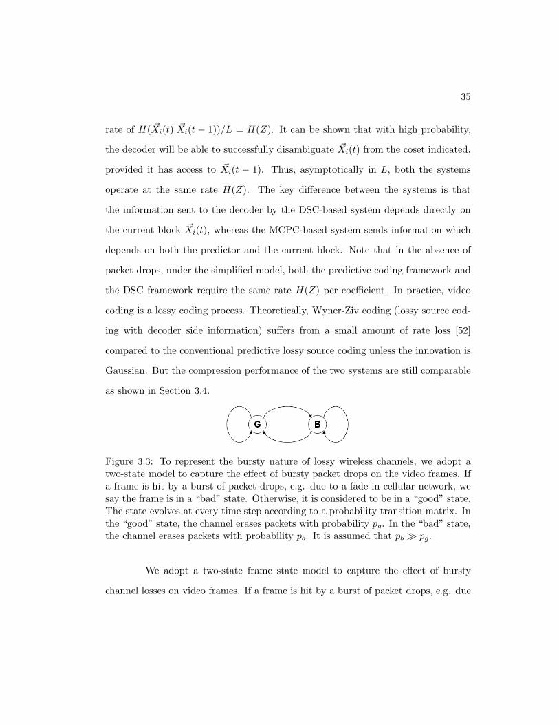
Figure 3.3: To represent the bursty nature of lossy wireless channels, we adopt atwo-state model to capture the effect of bursty packet drops on the video frames. Ifa frame is hit by a burst of packet drops, e.g. due to a fade in cellular network, wesay the frame is in a “bad” state. Otherwise, it is considered to be in a “good” state.The state evolves at every time step according to a probability transition matrix. Inthe “good” state, the channel erases packets with probability pg. In the “bad” state,the channel erases packets with probability pb. It is assumed that pb ≫ pg.
We adopt a two-state frame state model to capture the effect of bursty
channel losses on video frames. If a frame is hit by a burst of packet drops, e.g. due
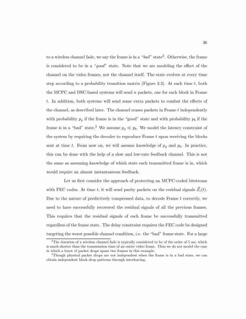
36
to a wireless channel fade, we say the frame is in a “bad” state2. Otherwise, the frame
is considered to be in a “good” state. Note that we are modeling the effect of the
channel on the video frames, not the channel itself. The state evolves at every time
step according to a probability transition matrix (Figure 3.3). At each time t, both
the MCPC and DSC-based systems will send n packets, one for each block in Frame
t. In addition, both systems will send some extra packets to combat the effects of
the channel, as described later. The channel erases packets in Frame t independently
with probability pg if the frame is in the “good” state and with probability pb if the
frame is in a “bad” state.3 We assume pg ≪ pb. We model the latency constraint of
the system by requiring the decoder to reproduce Frame t upon receiving the blocks
sent at time t. From now on, we will assume knowledge of pg and pb. In practice,
this can be done with the help of a slow and low-rate feedback channel. This is not
the same as assuming knowledge of which state each transmitted frame is in, which
would require an almost instantaneous feedback.
Let us first consider the approach of protecting an MCPC-coded bitstream
with FEC codes. At time t, it will send parity packets on the residual signals ~Zi(t).
Due to the nature of predictively compressed data, to decode Frame t correctly, we
need to have successfully recovered the residual signals of all the previous frames.
This requires that the residual signals of each frame be successfully transmitted
regardless of the frame state. The delay constraint requires the FEC code be designed
targeting the worst possible channel condition, i.e. the “bad” frame state. For a large
2The duration of a wireless channel fade is typically considered to be of the order of 5 ms, whichis much shorter than the transmission time of an entire video frame. Thus we do not model the casein which a burst of packet drops spans two frames in this example.
3Though physical packet drops are not independent when the frame is in a bad state, we canobtain independent block drop patterns through interleaving.
37
n, the rate required is at least
RFEC =H(Z)
1 − pb. (3.1)
This can be achieved by using maximum distance separable (MDS) codes, such as
the Reed-Solomon codes, as reviewed in Section 2.1.2.
The proposed DSC-based system takes a different approach in handling
packet drops. When the syndrome for a block is lost in a “bad” frame due to a
channel erasure, the decoder will not attempt to decode that block, but tries to
arrest the effects of such losses on future frames. Suppose Frame t−1 is in the “bad”
state but Frame t − 2 is entirely correctly reconstructed. Obviously, the predictor
blocks for some of the current blocks will be in error due to packet losses at time
t − 1. Let ~Xi(t) be one such block. The proposed DSC-based system tries to use
the next best predictor ~Xi(t− 2) from two frames ago as side information. However,
~Xi(t − 2) is of an inferior quality to ~Xi(t − 1). In order to successfully decode,
the decoder now requires the number of cosets to be 2H( ~Xi(t)| ~Xi(t−2)) instead of the
original 2H( ~Xi(t)| ~Xi(t−1)) = 2LH(Z). As reviewed in Section 2.1.3, this can be achieved
by further partitioning each of the original 2LH(Z) cosets into 2L(H(Z∗Z)−H(Z)) sub-
cosets. Here we defined Z ∗Z as the sum of two i.i.d. random variables with marginal
distributions pZ such that H( ~Xi(t)| ~Xi(t − 2)) = H(Z ∗ Z). In addition to the coset
information at rate H(Z), incremental syndrome to indicate the sub-coset at rate
H(Z ∗Z)−H(Z) is also required to be sent by the encoder. This is analogous to the
additional bit needed to decode from the inferior side information in the example in
38
Section 2.1.3. Thus, the rate needed by the DSC-based system is now
R =H(Z ∗ Z)
1 − pg(3.2)
=H(Z)
1 − pg+
H(Z ∗ Z) − H(Z)
1 − pg. (3.3)
The factor 11−pg
comes from the extra rate needed by an MDS code to protect these
coset indices against packet drops in a “good” frame state. The first term in (3.3) is
the bare minimum needed to ensure successful decoding if the frames are always in
the “good” state. The second term is the incremental information needed to combat
a burst of packet drops in Frame t−1. If the encoder adopts this scheme, then clearly
the decoder can recover block ~Xi(t) if either ~Xi(t − 1) or ~Xi(t − 2) is sent. This is
very similar to the flexible decoding technique proposed in [12] in spirit. However, we
can improve upon this scheme by taking advantage of the fact that not all blocks in
Frame t−1 are lost during transmission and not all blocks in Frame t need additional
syndrome to decode correctly.
Since only pb fraction of the blocks in Frame t − 1 are erroneously recon-
structed, only pb fraction of the blocks in Frame t will be decoded using predictors
in Frame t− 2 thereby needing incremental syndromes to be correctly decoded. The
other 1 − pb fraction of the blocks, whose predictors are not lost in Frame t − 1,
can be correctly decoded. Further, once they are correctly decoded, the incremental
syndromes for these blocks can be inferred. Therefore, even when no incremental
syndromes are sent, the decoder is able to recover 1 − pb fraction of these sub-coset
indices. Since the decoder also has knowledge of the location of the corrupted blocks,
it is as if the incremental syndromes went through an erasure channel with erasure
probability pb. This allows the encoder to send the incremental syndromes at a re-
39
duced rate by applying an erasure code over the sub-coset indices for all blocks in
Frame t and sending only the parity at rate pb(H(Z ∗ Z) − H(Z)). The total rate
needed can therefore be reduced to
RDSC =H(Z)
1 − pg+
pb(H(Z ∗ Z) − H(Z))
1 − pg. (3.4)
The rate difference between the pure FEC-based approach and the proposed
DSC-based approach is
∆R = RFEC − RDSC (3.5)
=pb(2H(Z) − H(Z ∗ Z))
1 − pg+
(p2b − pg)H(Z)
(1 − pb)(1 − pg). (3.6)
Since H(Z ∗ Z) ≤ 2H(Z), the difference is guaranteed to be positive for
pg < p2b . Using the proposed DSC-based strategy, the analysis holds as long as no
two consecutive frames are both in the “bad” state.
The philosophy behind the illustrative example can be easily extended to
the case where more than one frames can be hit by bursts of packet drops consecu-
tively. One solution is for each block to have more than two predictors and aim to
decode correctly as long as one of the predictors has been reconstructed correctly at
the decoder. For example, suppose at most two frames can be in the “bad” state
consecutively, the rate at which the encoder needs to operate is
RDSC =H(Z)
1 − pg+
pb(H(Z ∗ Z) − H(Z))
1 − pg+
p2b(H(Z ∗ Z ∗ Z) − H(Z ∗ Z))
1 − pg. (3.7)
Compared to (3.4), (3.7) has an additional third term, which is used to
decode the current block using the predictor in Frame t − 3 if both the predictor in
Frame t − 1 and the one in Frame t − 2 have been corrupted due to packet drops.
40
Clearly, as we increase the number of consecutive “bad” frames that the
system is designed to tolerate, the gain of the proposed approach decreases compared
to the FEC approach. In practice, we have to design for a certain outage probability.
An outage is defined as the event in which the number of consecutive “bad” frames
goes beyond what the encoder is designed for. From the real-world channel simulator
we obtained for the CDMA 2000 1x cellular network, we find it sufficient to associate
each block with only two predictors, as detailed in Section 3.4.
It is clear from this example that the proposed scheme is not always ad-
vantageous compared to the predictive coding scheme. First, if the channel does not
have a bursty nature, i.e. pg and pb are close, there is not necessarily a rate gain.
Second, we need the second predictor to be reasonably correlated to the current
block, i.e. we would like H(Z ∗ Z) − H(Z) to be small. The strong and typically
persistent temporal correlation unique to video data makes this possible.
Finite block length analysis: The rough argument above assumed a large num-
ber of packets n in each frame. This is not true for practical video transmission.
While the philosophy we presented in the illustrative example holds regardless of
the block length, the specific parameters for a practical system need to be adjusted
taking the block length n into consideration.
For example, suppose we want to use an erasure code to target erasure
probability p. The infinite block length analysis would suggest that we need an
overhead of np1−p
redundant packets such that all the packets can be recovered with
probability close to 1. However, this is not the case when n is small. In an extreme
example, suppose there are only 2 packets in a frame and the erasure probability is
0.5. We would transmit 2 redundant parity packets as prescribed by the infinite block
41
length analysis. With probability 116 , all four packets will be lost. With probability
14 , three out of four packets will be lost. In either case, there will be unrecoverable
packet drops. In fact, we need to send 8 redundant packets to ensure all the data
packets can be recovered with probability 0.99. The effect of finite block length will
affect both the choice of FEC used to guarantee packet delivery in a “good” frame
and the rebate factor we can get for the robustness layer.
Here, we use a more exact analysis of the dynamics for a small number of
packets n per frame. With a small n, both the FEC rate to use in a good frame
state and the rebate factor pb that we observe in the previous analysis are overly
optimistic for practical scenarios. This analysis will provide us with a guideline on
how to numerically obtain an appropriate set of parameters given fixed n, pg, and
pb. This finite block length analysis will also demonstrate the disadvantage of the
FEC-based approach when the delay constraint is stringent and FEC codes can be
applied only to a small number of blocks at a time.
All the codes are assumed to be be MDS. We compute the marginal proba-
bility of error in reproducing a packet at the decoder for a particular set of parame-
ters. This probability is conditional on the frame state sequence. Specifically, Xi(t)
will be in error if any of the following events happens:
• The packet containing Xi(t) is lost;
• The packet containing Xi(t) is received but both Xi(t − 1) and Xi(t − 2) are
in error;
• The packet containing Xi(t) is received, Xi(t − 1) is erroneous, Xi(t − 2) is
correct but the robustness layer for time t − 1 is not decodable, i.e. more
42
predictors are corrupted in Frame t − 1 than expected.
Using this, the probability of Xi(t) being in error can be recursively evalu-
ated for each frame state sequence. We can choose the parameters, namely the FEC
overhead in a “good” state and the rebate factor of the robustness layer, using any
desired criteria. For example, we can set a bound for the average probability of Xi(t)
being in error over a large number of state sequences. Though there is not a closed
form solution for the parameters as a function of the target error event probability,
we can numerically solve for them given a fixed block length n, pg, and pb. Note
that the decisions for the FEC overhead in a “good” state and the rebate factor of
the robustness layer are interdependent. Among all solutions that achieve the same
error event probability, we choose the one that is the most rate efficient.
Now we use an example to compare the performance of the proposed system
to the one in which predictively coded data is protected with MDS FEC. We compute
and compare the probability of the decoder failing to recover a video block as a
function of time under a typical channel state sequence. We choose our parameters
to closely match the simulation setup presented in Section 3.4 to get a sense of the
expected performance. Based on the practical error masks used in the Section 3.4,
we set pg = 0.03, pb = 0.3. The frame state is “bad” at times t = 6, 17, 38, and
“good” at other times. We choose n = 30 which is a realistic value for the packets
per frame. We assume a binary field with a Bernoulli innovation process Z, i.e.
Pr(Z = 1) = 1 − Pr(Z = 0) = p.
We use p = 0.11, which corresponds to a rate of H(Z) = 0.5 and H(Z ∗ Z) = 0.71.
The long block length analysis would suggests pb(H(Z ∗Z)−H(Z)) = 0.063
bit/symbol for the sub-coset indices, which is 12.6% of the baseline coset indices.
43
Here, we choose the rate for the sub-coset indices to be 26% of the baseline infor-
mation instead to target a certain block recovery probability. For comparison, we
consider two conventional predictive coding systems which use MDS FEC: one op-
erates at the same overall rate as the DSC-based system by using 26% extra rate for
FEC, and the other uses 70% extra rate for FEC. Figure 3.4 shows that the proposed
system has a high block recovery failure rate for frames in a “bad” state, but can
immediately improve performance in the following “good” state. In fact, under the
same latency constraint, to deliver similar performance under “good” frame state as
the proposed DSC-based system, an MCPC-based system protected with MDS FEC
needs 70% extra rate for the FEC. This difference is even bigger when the block
length n becomes smaller.
3.3 System implementation
We implement a practical DSC-based video coder built upon the intuition
from the illustrative example. Just like in the illustrative example, each encoding
block is associated with two predictors. We design to successfully decode as long
as at least one of these predictors is correctly reconstructed at the decoder. The
compressed bitstream consists of a baseline layer and a robustness layer. The baseline
layer contains syndromes to reconstruct each block using the best predictor. It
suffices to reconstruct the entire video perfectly when the compressed bitstream
is transmitted without error. The robustness layer contains additional incremental
syndromes. When combined with the baseline syndrome, these robustness syndromes
can decode blocks using the second best predictors, as long as the fraction of blocks
whose best predictors are not available is within a designed threshold. We now detail
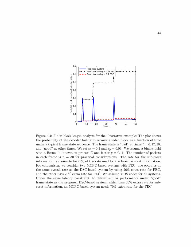
44
0 10 20 30 40 50 600
0.1
0.2
0.3
0.4
0.5
0.6
0.7
Time t
Pro
bability
ofvid
eoblo
ckdis
pla
yfa
ilure
Proposed systemPredictive coding + 0.26 FECPredictive coding + 0.7 FEC
Figure 3.4: Finite block length analysis for the illustrative example: The plot showsthe probability of the decoder failing to recover a video block as a function of timeunder a typical frame state sequence. The frame state is “bad” at times t = 6, 17, 38,and “good” at other times. We set pb = 0.3 and pg = 0.03. We assume a binary fieldwith a Bernoulli innovation process Z and factor p = 0.11. The number of packetsin each frame is n = 30 for practical considerations. The rate for the sub-cosetinformation is chosen to be 26% of the rate used for the baseline coset information.For comparison, we consider two MCPC-based systems with FEC: one operates atthe same overall rate as the DSC-based system by using 26% extra rate for FEC,and the other uses 70% extra rate for FEC. We assume MDS codes for all systems.Under the same latency constraint, to deliver similar performance under “good”frame state as the proposed DSC-based system, which uses 26% extra rate for sub-coset information, an MCPC-based system needs 70% extra rate for the FEC.
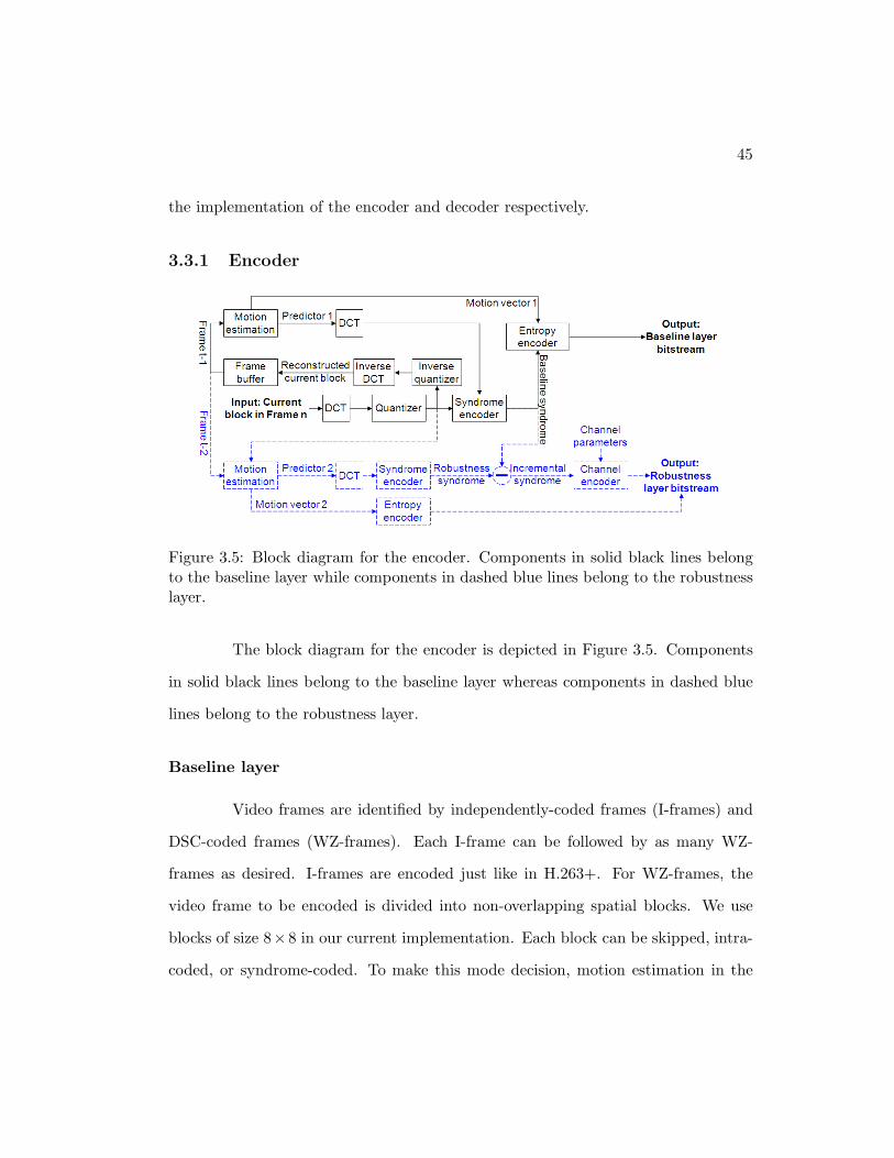
45
the implementation of the encoder and decoder respectively.
3.3.1 Encoder
Figure 3.5: Block diagram for the encoder. Components in solid black lines belongto the baseline layer while components in dashed blue lines belong to the robustnesslayer.
The block diagram for the encoder is depicted in Figure 3.5. Components
in solid black lines belong to the baseline layer whereas components in dashed blue
lines belong to the robustness layer.
Baseline layer
Video frames are identified by independently-coded frames (I-frames) and
DSC-coded frames (WZ-frames). Each I-frame can be followed by as many WZ-
frames as desired. I-frames are encoded just like in H.263+. For WZ-frames, the
video frame to be encoded is divided into non-overlapping spatial blocks. We use
blocks of size 8×8 in our current implementation. Each block can be skipped, intra-
coded, or syndrome-coded. To make this mode decision, motion estimation in the

46
pixel domain is carried out to locate the best predictor in the reconstructed reference
frame. The mean square error between the current block and the best predictor will
determine whether the block will be skipped, intra-coded or syndrome-coded. Skip
and intra blocks are encoded the same way as in H.263+. To syndrome-code the ith
block in the tth frame, the following steps are followed.
• DCT: Take DCT of both the current block and the best predictor block. We
denote the non-quantized DCT coefficients of the current block and its motion-
compensated predictor by {Xji (t)}64
j=1 and {Xj′
i (t − 1)}64j=1, respectively.
• Quantization: Quantize the DCT coefficients of the current block {Xji (t)}64
j=1
to {Xji (t)}64
j=1 using a scalar quantizer.
• Syndrome coding: Generate syndrome for {Xji (t)}64
j=1 using the multi-level
coding scheme [45] as described in Section 2.1.3. Recall that for each DCT
coefficient, its syndrome consists of the least significant bits of its binary rep-
resentation that cannot be inferred from the side information. For the jth
coefficient of this block, the number of least significant bits of the binary rep-
resentation of Xji (t) that need to be sent can be computed as
Lji (t − 1) = max
0,
log2
∣
∣
∣Xji (t) − Xj′
i (t − 1)∣
∣
∣
∆
+ 1
,
where ∆ is the quantization step size determined by the desired video quality.
For example, let the DC coefficient of the ith block in the tth frame be 156. Let
the quantization step size be 10. Therefore X1i (t) = 160, whose label is 16 in
decimal and 10000 in binary. Let the DC coefficient of the motion-compensated
predictor for this block in Frame t−1 be 142. The number of bit planes needed

47
is therefore 2 and these bits are “00”. Theoretically, the correlation between the
source and the side information is known at both the encoder and the decoder.
Thus both the encoder and the decoder would know that two bits need to be
sent for this coefficient. However, this is not the case in practice. The encoder
needs to indicate to the decoder both the number of bit planes to send, which
essentially describes the correlation statistics, and what those bits are. We
use a standard variable length coding technique to map this information to a
unique symbol.
• Entropy coding: The symbols of all the DCT coefficients’ syndromes within
a block are zig-zag scanned, run-length coded and then arithmetic coded (sum-
marized as Entropy Coding in the block diagram). The motion vectors within
each slice are differentially coded just like in H.26x4.
• FEC coding: Finally, an MDS FEC code is applied to the base layer to
combat packet drops when the frame is in the “good” state. If the “good”
state packet drop rate is sufficiently low, this layer of protection is optional.
• Reconstruction: Inverse quantization, inverse DCT and estimation is carried
out to generate the encoder reconstruction of the current block, which is in turn
written back to frame memory.
The resulting compressed bitstream corresponds to the first term in (3.4).
This is the bare minimum rate needed when the frames are in the “good” state all
the time.
4We preserve independent decodability of a slice.
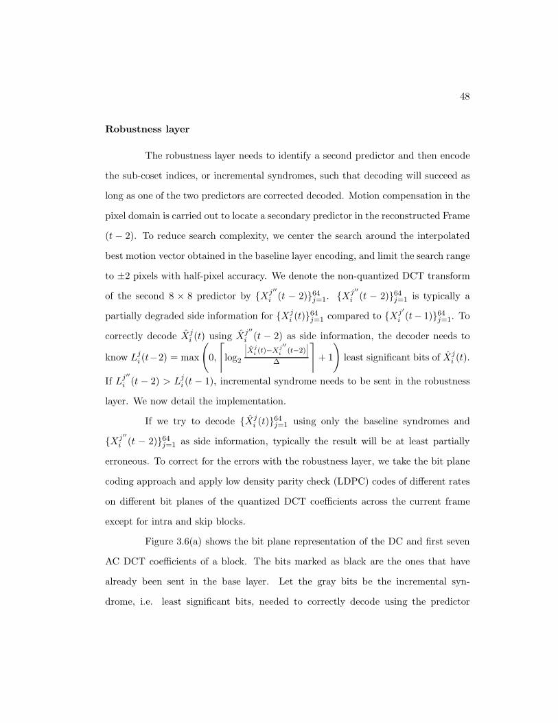
48
Robustness layer
The robustness layer needs to identify a second predictor and then encode
the sub-coset indices, or incremental syndromes, such that decoding will succeed as
long as one of the two predictors are corrected decoded. Motion compensation in the
pixel domain is carried out to locate a secondary predictor in the reconstructed Frame
(t − 2). To reduce search complexity, we center the search around the interpolated
best motion vector obtained in the baseline layer encoding, and limit the search range
to ±2 pixels with half-pixel accuracy. We denote the non-quantized DCT transform
of the second 8 × 8 predictor by {Xj′′
i (t − 2)}64j=1. {Xj′′
i (t − 2)}64j=1 is typically a
partially degraded side information for {Xji (t)}64
j=1 compared to {Xj′
i (t− 1)}64j=1. To
correctly decode Xji (t) using Xj′′
i (t − 2) as side information, the decoder needs to
know Lji (t−2) = max
(
0,
⌈
log2
∣
∣
∣Xji (t)−X
j′′
i (t−2)∣
∣
∣
∆
⌉
+ 1
)
least significant bits of Xji (t).
If Lj′′
i (t − 2) > Lji (t − 1), incremental syndrome needs to be sent in the robustness
layer. We now detail the implementation.
If we try to decode {Xji (t)}64
j=1 using only the baseline syndromes and
{Xj′′
i (t − 2)}64j=1 as side information, typically the result will be at least partially
erroneous. To correct for the errors with the robustness layer, we take the bit plane
coding approach and apply low density parity check (LDPC) codes of different rates
on different bit planes of the quantized DCT coefficients across the current frame
except for intra and skip blocks.
Figure 3.6(a) shows the bit plane representation of the DC and first seven
AC DCT coefficients of a block. The bits marked as black are the ones that have
already been sent in the base layer. Let the gray bits be the incremental syn-
drome, i.e. least significant bits, needed to correctly decode using the predictor
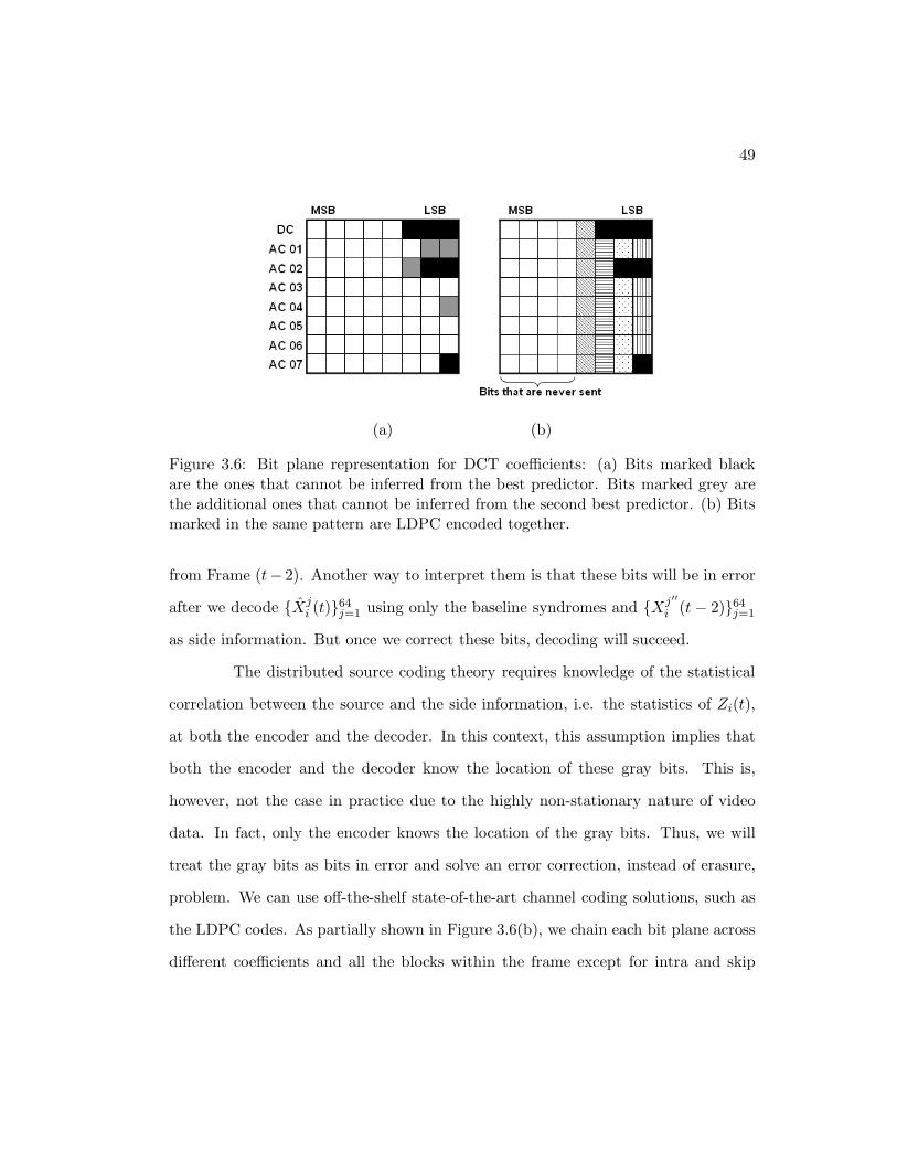
49
(a) (b)
Figure 3.6: Bit plane representation for DCT coefficients: (a) Bits marked blackare the ones that cannot be inferred from the best predictor. Bits marked grey arethe additional ones that cannot be inferred from the second best predictor. (b) Bitsmarked in the same pattern are LDPC encoded together.
from Frame (t− 2). Another way to interpret them is that these bits will be in error
after we decode {Xji (t)}64
j=1 using only the baseline syndromes and {Xj′′
i (t − 2)}64j=1
as side information. But once we correct these bits, decoding will succeed.
The distributed source coding theory requires knowledge of the statistical
correlation between the source and the side information, i.e. the statistics of Zi(t),
at both the encoder and the decoder. In this context, this assumption implies that
both the encoder and the decoder know the location of these gray bits. This is,
however, not the case in practice due to the highly non-stationary nature of video
data. In fact, only the encoder knows the location of the gray bits. Thus, we will
treat the gray bits as bits in error and solve an error correction, instead of erasure,
problem. We can use off-the-shelf state-of-the-art channel coding solutions, such as
the LDPC codes. As partially shown in Figure 3.6(b), we chain each bit plane across
different coefficients and all the blocks within the frame except for intra and skip
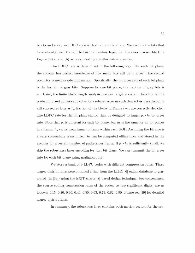
50
blocks and apply an LDPC code with an appropriate rate. We exclude the bits that
have already been transmitted in the baseline layer, i.e. the ones marked black in
Figure 3.6(a) and (b) as prescribed by the illustrative example.
The LDPC rate is determined in the following way. For each bit plane,
the encoder has perfect knowledge of how many bits will be in error if the second
predictor is used as side information. Specifically, the bit error rate of each bit plane
is the fraction of gray bits. Suppose for one bit plane, the fraction of gray bits is
pe. Using the finite block length analysis, we can target a certain decoding failure
probability and numerically solve for a rebate factor hb such that robustness decoding
will succeed as long as hb fraction of the blocks in Frame t− 1 are correctly decoded.
The LDPC rate for the bit plane should then be designed to target pe · hb bit error
rate. Note that pe is different for each bit plane, but hb is the same for all bit planes
in a frame. hb varies from frame to frame within each GOP. Assuming the I-frame is
always successfully transmitted, hb can be computed offline once and stored in the
encoder for a certain number of packets per frame. If pe · hb is sufficiently small, we
skip the robustness layer encoding for that bit plane. We can transmit the bit error
rate for each bit plane using negligible rate.
We store a bank of 9 LDPC codes with different compression rates. These
degree distributions were obtained either from the LTHC [6] online database or gen-
erated (in [39]) using the EXIT charts [8] based design technique. For convenience,
the source coding compression rates of the codes, to two significant digits, are as
follows: 0.15, 0.20, 0.30, 0.40, 0.50, 0.63, 0.73, 0.82, 0.90. Please see [39] for detailed
degree distributions.
In summary, the robustness layer contains both motion vectors for the sec-
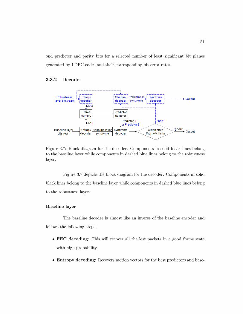
51
ond predictor and parity bits for a selected number of least significant bit planes
generated by LDPC codes and their corresponding bit error rates.
3.3.2 Decoder
Figure 3.7: Block diagram for the decoder. Components in solid black lines belongto the baseline layer while components in dashed blue lines belong to the robustnesslayer.
Figure 3.7 depicts the block diagram for the decoder. Components in solid
black lines belong to the baseline layer while components in dashed blue lines belong
to the robustness layer.
Baseline layer
The baseline decoder is almost like an inverse of the baseline encoder and
follows the following steps:
• FEC decoding: This will recover all the lost packets in a good frame state
with high probability.
• Entropy decoding: Recovers motion vectors for the best predictors and base-
52
line syndromes for DCT coefficients.
• Syndrome decoding: Based on decoder’s knowledge regarding past packet
drop history, syndrome decode a block if its best predictor has been correctly
decoded. Since a predictor block could overlap with up to four 8 × 8 non-
overlapping encoding blocks, it will be considered correctly decoded only if all
these overlapping encoding blocks have been correctly decoded. The decoder
syndrome-decodes each coefficient to be the codeword closest to the side infor-
mation in the indicated coset. This step also includes an estimation process at
the end that is standard to Wyner-Ziv decoding to exact estimation gain. For
each block whose best predictor is available, the decoder marks the block as
correct. Otherwise, it marks the block as uncertain and leaves the decoding to
the robustness layer.
• Inverse quantization.
• Inverse DCT.
Clearly, if there are no packet drops, baseline layer decoding suffices to
reconstruct the entire video.
Robustness layer
If the current frame is in a bad state, the lost packets cannot be recovered
in general. We carry out standard error concealment and mark these blocks as lost.
We will not attempt robustness layer decoding either as prescribed by the illustrative
example. If the frame is a good state, and there are past errors to clean up due to
previous bad frame states, robustness layer decoding works as follows:
53
• Entropy decoding: Recover the motion vectors for the second predictor.
• Syndrome decoding for uncertain blocks: For each block whose best
predictor is not available, if the second predictor has been correctly decoded,
syndrome-decode this block using only the baseline syndrome with the second
predictor being the side information. If neither of the predictors is correctly
decoded, the best predictor, though corrupted, is used as side information to
syndrome-decode the block using only the baseline syndrome.
• Syndrome decoding to clean up past errors: After syndrome-decoding
the whole frame once, we use the partially erroneous reconstruction (in DCT
domain) as the side information to the robustness layer decoder. Starting from
the least significant bit plane, we carry out bit plane decoding using the LDPC
parity bits in the robustness layer. After each LDPC decoding, each block
that is mark uncertain is syndrome-decoded on a coefficient-basis again (using
possibly newly corrected syndromes). The result is used as side information
for the decoding of the next bit plane. If all LDPC decoding succeeds, which
should happen with high probability, all the uncertain blocks are re-marked as
correct.
• Estimation, inverse quantization and inverse DCT for blocks that changed
status from uncertain to correct.
One significant advantage of such a layered approach is that starting with a
new I-frame, the decoder does not need the robustness layer at all until it experiences
a bad frame state. This greatly reduces overall decoding complexity as the base layer
is entropy-coded and multi-level syndrome decoding has very low complexity.
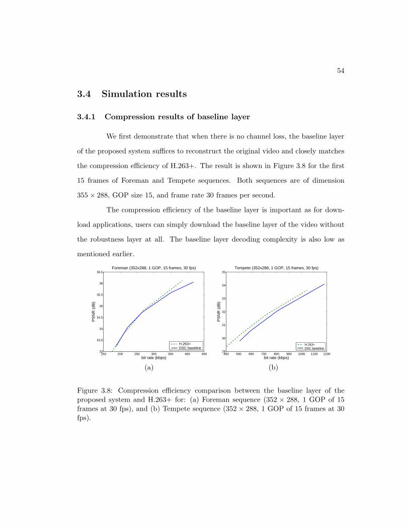
54
3.4 Simulation results
3.4.1 Compression results of baseline layer
We first demonstrate that when there is no channel loss, the baseline layer
of the proposed system suffices to reconstruct the original video and closely matches
the compression efficiency of H.263+. The result is shown in Figure 3.8 for the first
15 frames of Foreman and Tempete sequences. Both sequences are of dimension
355 × 288, GOP size 15, and frame rate 30 frames per second.
The compression efficiency of the baseline layer is important as for down-
load applications, users can simply download the baseline layer of the video without
the robustness layer at all. The baseline layer decoding complexity is also low as
mentioned earlier.
150 200 250 300 350 400 45033
33.5
34
34.5
35
35.5
36
36.5
bit rate (kbps)
PS
NR
(dB
)
Foreman (352x288, 1 GOP, 15 frames, 30 fps)
H.263+DSC baseline
400 500 600 700 800 900 1000 1100 120029
30
31
32
33
34
35
bit rate (kbps)
Tempete (352x288, 1 GOP, 15 frames, 30 fps)
PS
NR
(dB
)
H.263+DSC baseline
(a) (b)
Figure 3.8: Compression efficiency comparison between the baseline layer of theproposed system and H.263+ for: (a) Foreman sequence (352 × 288, 1 GOP of 15frames at 30 fps), and (b) Tempete sequence (352 × 288, 1 GOP of 15 frames at 30fps).

55
3.4.2 Robustness results of robustness layer
We now demonstrate the effect of the robustness layer for low-latency trans-
mission over channels with bursty errors. Three systems are compared:
1. Proposed system with its baseline layer encoded at rate R and the robustness
layer at rate ∆R,
2. H.263+ encoded at rate R′ such that the decoded video quality is the same as
that of System (1) when there are no packet drops and R + ∆R−R′ allocated
to FEC (we use Reed-Solomon codes),
3. H.263+ encoded at rate R + ∆R with random intra refresh enabled such that
the decoded video quality is the same as that of System (1) when there are no
packet drops.
The latency constraint is 1 frame, as in, the decoder must immediately display the
received frame.
Two-state channel
First, we simulate the same two-state channel model as described in Sec-
tion 3.2. In the “good” state, we simulate 3% independent packet drops. In the “bad”
state, we simulate 30% independent packet drops. We used high-motion sequences
as they are the most prone to the effect of drift and present the biggest challenges
in robust video transmission. We use the Stefan sequence (352× 240, GOP = 15, 15
fps) with R = 1.1mbps and ∆R = 360kbps and Football sequence (352 × 240, GOP
= 30, 15 fps) with R = 900kbps and ∆R = 300kbps.
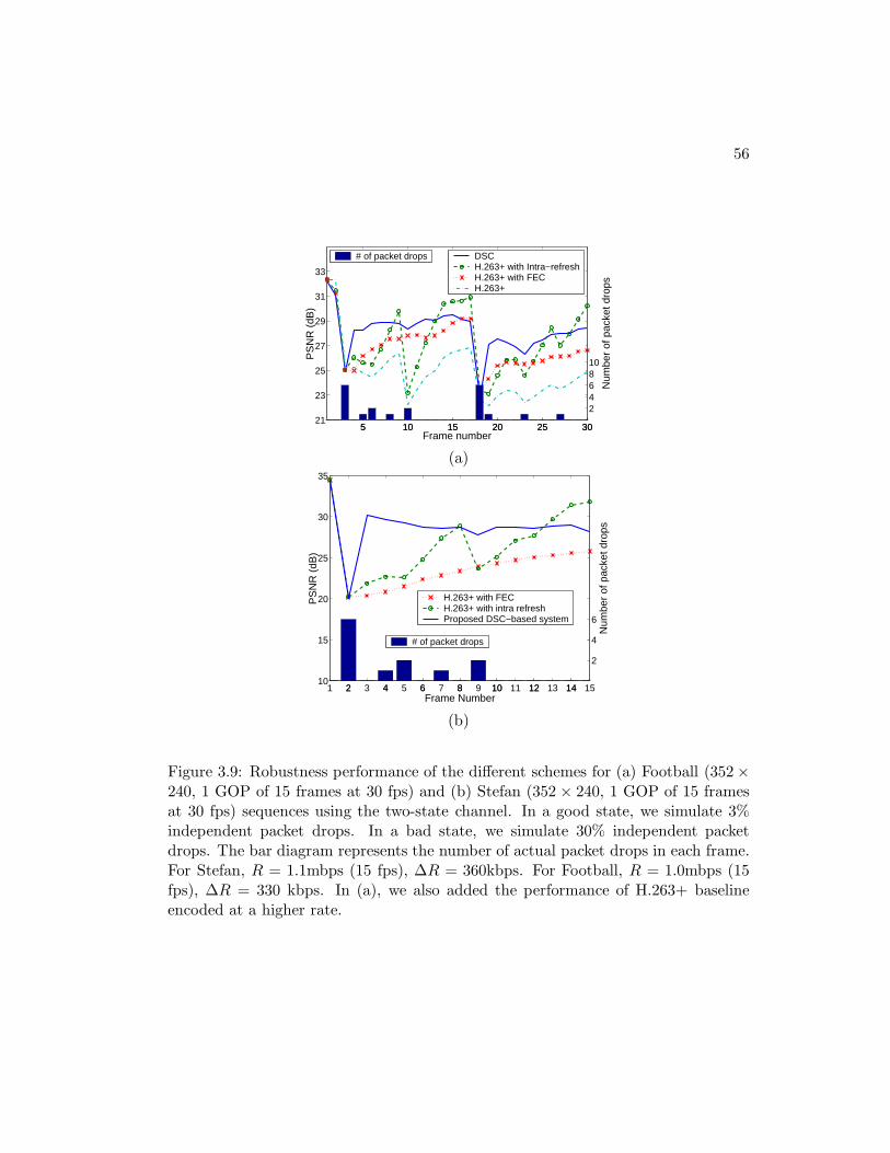
56
5 10 15 20 25 3021
23
25
27
29
31
33
PS
NR
(dB
)
Frame number5 10 15 20 25 30
246810
Num
ber
of p
acke
t dro
ps
DSCH.263+ with Intra−refreshH.263+ with FECH.263+
# of packet drops
(a)
2 4 6 8 10 12 1410
15
20
25
30
35
PS
NR
(dB
)
1 2 3 4 5 6 7 8 9 10 11 12 13 14 15
2
4
6
Frame Number
Num
ber
of p
acke
t dro
psH.263+ with FECH.263+ with intra refreshProposed DSC−based system
# of packet drops
(b)
Figure 3.9: Robustness performance of the different schemes for (a) Football (352 ×240, 1 GOP of 15 frames at 30 fps) and (b) Stefan (352 × 240, 1 GOP of 15 framesat 30 fps) sequences using the two-state channel. In a good state, we simulate 3%independent packet drops. In a bad state, we simulate 30% independent packetdrops. The bar diagram represents the number of actual packet drops in each frame.For Stefan, R = 1.1mbps (15 fps), ∆R = 360kbps. For Football, R = 1.0mbps (15fps), ∆R = 330 kbps. In (a), we also added the performance of H.263+ baselineencoded at a higher rate.
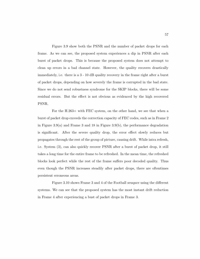
57
Figure 3.9 show both the PSNR and the number of packet drops for each
frame. As we can see, the proposed system experiences a dip in PSNR after each
burst of packet drops. This is because the proposed system does not attempt to
clean up errors in a bad channel state. However, the quality recovers drastically
immediately, i.e. there is a 3 - 10 dB quality recovery in the frame right after a burst
of packet drops, depending on how severely the frame is corrupted in the bad state.
Since we do not send robustness syndrome for the SKIP blocks, there will be some
residual errors. But the effect is not obvious as evidenced by the high recovered
PSNR.
For the H.263+ with FEC system, on the other hand, we see that when a
burst of packet drop exceeds the correction capacity of FEC codes, such as in Frame 2
in Figure 3.9(a) and Frame 3 and 18 in Figure 3.9(b), the performance degradation
is significant. After the severe quality drop, the error effect slowly reduces but
propagates through the rest of the group of picture, causing drift. While intra refresh,
i.e. System (3), can also quickly recover PSNR after a burst of packet drop, it still
takes a long time for the entire frame to be refreshed. In the mean time, the refreshed
blocks look perfect while the rest of the frame suffers poor decoded quality. Thus
even though the PSNR increases steadily after packet drops, there are oftentimes
persistent erroneous areas.
Figure 3.10 shows Frame 3 and 4 of the Football seuqnce using the different
systems. We can see that the proposed system has the most instant drift reduction
in Frame 4 after experiencing a bust of packet drops in Frame 3.
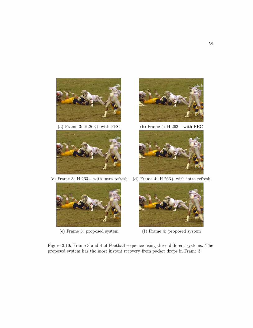
58
(a) Frame 3: H.263+ with FEC (b) Frame 4: H.263+ with FEC
(c) Frame 3: H.263+ with intra refresh (d) Frame 4: H.263+ with intra refresh
(e) Frame 3: proposed system (f) Frame 4: proposed system
Figure 3.10: Frame 3 and 4 of Football sequence using three different systems. Theproposed system has the most instant recovery from packet drops in Frame 3.
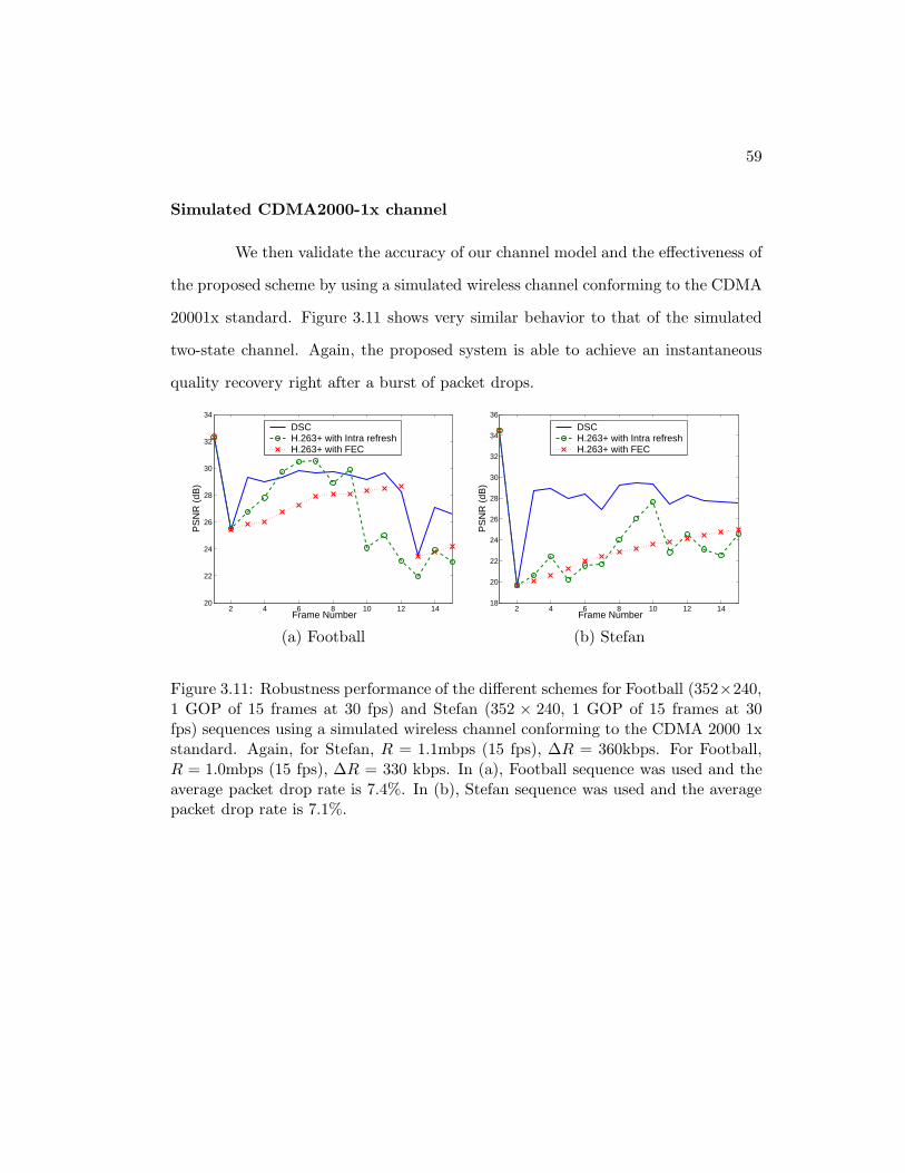
59
Simulated CDMA2000-1x channel
We then validate the accuracy of our channel model and the effectiveness of
the proposed scheme by using a simulated wireless channel conforming to the CDMA
20001x standard. Figure 3.11 shows very similar behavior to that of the simulated
two-state channel. Again, the proposed system is able to achieve an instantaneous
quality recovery right after a burst of packet drops.
2 4 6 8 10 12 1420
22
24
26
28
30
32
34
Frame Number
PS
NR
(dB
)
DSCH.263+ with Intra refreshH.263+ with FEC
2 4 6 8 10 12 1418
20
22
24
26
28
30
32
34
36
Frame Number
PS
NR
(dB
)
DSCH.263+ with Intra refreshH.263+ with FEC
(a) Football (b) Stefan
Figure 3.11: Robustness performance of the different schemes for Football (352×240,1 GOP of 15 frames at 30 fps) and Stefan (352 × 240, 1 GOP of 15 frames at 30fps) sequences using a simulated wireless channel conforming to the CDMA 2000 1xstandard. Again, for Stefan, R = 1.1mbps (15 fps), ∆R = 360kbps. For Football,R = 1.0mbps (15 fps), ∆R = 330 kbps. In (a), Football sequence was used and theaverage packet drop rate is 7.4%. In (b), Stefan sequence was used and the averagepacket drop rate is 7.1%.
60
Chapter 4
Conclusion and future work
In this part of the thesis, we have focused on the problem of low-latency
video streaming over lossy packet networks. We have presented a distributed source
coding based video coding system that enables robust low-latency video transmis-
sion over channels characterized by bursty packet drops, such as wireless networks.
Based on a generalization of the classical Wyner-Ziv setup, the proposed distributed
video codec is characterized by an inherent system uncertainty about the “state” of
the relevant side information available at the decoder. The compressed bitstream
comprises of a baseline layer that suffices to reconstruct the video when there are
no packet drops and a robustness layer that is used to combat transmission errors.
By taking a joint source-channel coding approach, the proposed system can tune to
both the source content as well as to the network loss characteristics.
The key ideas of the proposed system are the following:
• We choose to give up perfectly reconstructing frames that are transmitted under
poor channel conditions. Instead, we aim to recover decoded video quality

61
immediately after a burst of packet drops.
• We associate each block with more than one predictors and aim to decode
successfully as long as one of these predictors are correctly reconstructed at the
decoder. The strong temporal correlation of video data provides the perfect
diversity in time to make this scheme efficient.
• Instead of coding according to the worst predictor that the current block is
associated with, we take advantage of the fact that the best predictor will
be available at the decoder most of the time and achieve better compression
efficiency.
• The decoder can make intelligent choice regarding which predictor to use based
on its knowledge of previous blocks’ decoding status.
While some of these philosophies can be used in the conventional predictive
coding framework as well, the distributed source coding framework allows the most
efficient implementation of these ideas in terms of compression efficiency for lossy
coding. In this thesis, we have presented a theoretical analysis of the proposed
system under a simplified analytically tractable model and quantified the gains with
respect to predictive codecs when the transmission channel is characterized by bursty
packet drops. We implemented the proposed system and verified its effectiveness of
the proposed system through simulations using both synthetic and real-world channel
simulators.
The work in this part of the thesis suggests several avenues of further study.
We itemize some of these directions here.

62
• The robustness advantages of the proposed system need to be studied for more
accurate video models.
• By using rate-adaptive LDPC codes for the robustness layer, one may break
the robustness layer into several layers to target different packet drop statistics.
This may be useful in a layered multicast setup, like in [30].
• For a video coder, there is typically a complexity-performance tradeoff. In the
context of the proposed system, coarser motion search will naturally lead to
lower compression efficiency. However, in a DSC framework, this means that
predictors of worse quality will also lead to correct reconstruction of the current
block. It is worthwhile to study how to exploit and quantify this increased
robustness with lower encoder complexity.
• Correlation estimation under arbitrary channel conditions remains an open
question in general.
We hope this work will spur further research in the area of robust video
transmission using distributed source coding principles. We believe the DSC frame-
work has the potential of leading to video codecs that are fundamentally more suit-
able for the new generation of video applications.
63
Part II
Video distribution over
collaborative peer-to-peer
networks

64
Chapter 5
Introduction
Internet video is poised to be the next big thing. It is predicted that the
revenue from Internet video will grow with an annual growth rate of 49.7% from
$0.63 billion in 2006 to $4.74 billion by 2011 [22]. As consumers spend more and
more time watching videos online, they are no longer content with being restrained
to their computers. Consequently, the demand to get Internet video into the living
room is at a record-high. This demand fuels the increasing popularity of services
(Amazon Unbox, Netflix On Demand, etc.), as well as devices with such capabilities
(Microsoft Media Center, Apple TV, TiVo, etc.). Once in the living room, consumers
quickly realize that they prefer to go beyond YouTube’s limited quality and enjoy
SD or even HD video.
However, providing high-quality Internet video with a traditional client-
server model is very costly [31]. The ever mounting demand is adding significant
pressure to existing server-based infrastructures, such as data centers and content
distribution networks (CDNs), which are already heavily burdened. As a result, high-
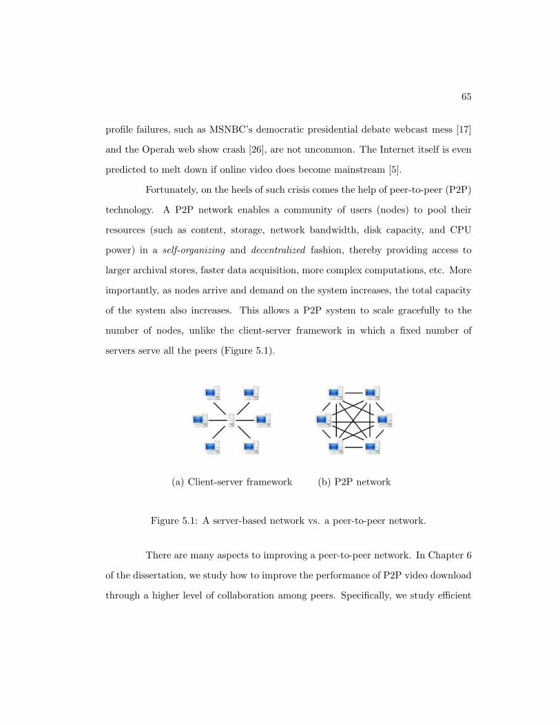
65
profile failures, such as MSNBC’s democratic presidential debate webcast mess [17]
and the Operah web show crash [26], are not uncommon. The Internet itself is even
predicted to melt down if online video does become mainstream [5].
Fortunately, on the heels of such crisis comes the help of peer-to-peer (P2P)
technology. A P2P network enables a community of users (nodes) to pool their
resources (such as content, storage, network bandwidth, disk capacity, and CPU
power) in a self-organizing and decentralized fashion, thereby providing access to
larger archival stores, faster data acquisition, more complex computations, etc. More
importantly, as nodes arrive and demand on the system increases, the total capacity
of the system also increases. This allows a P2P system to scale gracefully to the
number of nodes, unlike the client-server framework in which a fixed number of
servers serve all the peers (Figure 5.1).
(a) Client-server framework (b) P2P network
Figure 5.1: A server-based network vs. a peer-to-peer network.
There are many aspects to improving a peer-to-peer network. In Chapter 6
of the dissertation, we study how to improve the performance of P2P video download
through a higher level of collaboration among peers. Specifically, we study efficient
66
resource utilization of helper nodes. These are nodes that are not interested in
the file being shared but have spare bandwidth resources and are willing to share.
We propose a light-weight, distributed protocol that is backwards-compatible with
the popular BitTorrent file sharing protocol and analyze the steady-state system
performance using a fluid model as in Qiu and Srikant [38]. We then extend the
framework to design an algorithm for efficient utilization of helpers for P2P live
video multicast.
Throughout this part of dissertation, the terms “node”, “peer”, and “user”
are used interchangeably, according to the context, to refer to the entities that are
connected in a P2P network.
5.1 Peer-to-peer networking overview
Definition The definition for “peer-to-peer” can vary depending on the broadness
that is attached to the term. The strictest definitions of “pure” peer-to-peer refer to
totally distributed systems, in which all nodes are completely equivalent in terms of
functionality and tasks they perform. In the context of this dissertation, we adopt
a broader and widely accepted definition in [42], “peer-to-peer is a class of applica-
tions that take advantage of resources – storage, cycles, content, human presence –
available at the edges of the internet.”
Classification by application Peer-to-peer architectures have been employed for
various application categories, which include, but are not limited to, the following.
• Collaboration and Communication. This category includes systems that pro-
vide the infrastructure for facilitating direct, usually real-time, communication
67
and collaboration between peer computers. One of the most well-known exam-
ples is the Internet telephone company Skype [4].
• Distributed Computation. This category includes systems whose aim is to
take advantage of the available peer processing power, i.e. CPU cycles. This is
achieved by breaking down a computational intensive task into small work units
and distributing them to different peer computers. Peer computers execute
their corresponding work unit and return the results. Central coordination is
required for breaking up and distributing the tasks, as well as collecting the
results. Examples of such systems include Berkeley’s SETI@home project [3]
and distributed.net, which is a world-wide distributed computing effort that is
attempting to solve large scale problems using otherwise idle CPU time.
• Content Distribution. Most of the current P2P systems fall within the category
of content distribution, which includes systems and infrastructures designed for
the sharing of digital media and other data between users. Peer-to-peer con-
tent distribution systems range from relatively simple direct file-sharing appli-
cations to more sophisticated systems that create a distributed storage medium
for publishing, organizing, indexing, searching, updating, and retrieving data.
There are numerous such systems and infrastructures, including Gnutella [1],
KaZaA [2], and BitTorrent [14].
In this section, we review content distribution over P2P networks. The op-
eration of any P2P content distribution system relies on a network of peer computers
and connections among them. This network is formed on top of – and independently
from – the underlying physical computer network, and is thus referred to as an “over-
68
lay” network. Overlay networks can be distinguished in terms of their centralization
and structure.
Classification by degree of overlay centralization There are three types of
P2P architectures based on the degree of centralization of the overlay network: purely
decentralized architecture, partially centralized architecture, and hybrid decentral-
ized architecture. In a purely decentralized architecture, all nodes in the network
perform exactly the same tasks, acting both as servers and clients, and there is no
central coordination of their activities. The basis of a partially centralized architec-
ture is the same as with purely decentralized systems. Some of the nodes, however,
assume a more important role, such as acting as local central indices for files shared
by local peers. These so-called “supernodes” are assigned various roles by the net-
work depending on the application. These supernodes do not constitute single points
of failure for a P2P network, since they are dynamically assigned and, if they fail,
the network will automatically take action to replace them with others. Finally, in a
hybrid decentralized architecture, there is a central server facilitating the interaction
among peers by maintaining directories of participating peers, content metadata,
and sometimes the content source itself. Although the end-to-end interaction and
file exchanges may take place directly between two peer nodes, the central servers
facilitate this interaction by performing the lookups and identifying the nodes that
are sharing the relevant content.
Classification by overlay structure Unstructured overlays build a random graph
and use flooding or random walks on that graph to discover data stored by overlay
nodes. Structured overlays assign keys to data items and build a graph that maps
69
each key to the node that stores the corresponding data. While structured overlays
can provide guarantees on quality of service, e.g. the maximum number of hops to
locate the desired content, unstructured overlays are widely used in popular appli-
cations, such as Gnutella and BitTorrent. This is because unstructured overlays are
easy to maintain, resistent to peer churning, and can perform arbitrarily complex
queries.
In this dissertation we study two important forms of Internet video distri-
bution: download (e.g. downloads at iTunes store) and live multicast (e.g. NBC’s
web broadcast of the 2008 Olympic games). Each distribution method has its own
unique characteristics.
For download, peers aim to obtain a certain file that is pre-generated. Peers
may start the download any time they want, quit any time they want, and may
finish downloading at different times. From an end user’s point of view, the main
performance metric is the amount of time it takes to download the entire file.
For multicast, peers may join the system at different times but they watch
the same content at the same time. In other words, peers have synchronous or at
least loosely synchronous playback points. The content can be either pre-generated
or being generated in real-time. Nonetheless, unlike download, there is not a finishing
point for live multicast. Peers can stay in the system for as long as they want and
the content they are viewing is constantly updated.
The biggest difference between P2P download and streaming applications
is that for streaming applications, each packet has a specific delivery deadline. This
difference dictates that streaming applications need to have more efficient resource
allocation and topology building schemes. We will examine these topics in more

70
detail in Section 6.3.3.
71
Chapter 6
Helper-assisted peer-to-peer
video distribution
In this chapter, we study how to improve the performance of P2P video
download through a higher-level collaboration among peers. Specifically, we study
efficient resource utilization of helpers, which are nodes that are not interested in the
file being shared but are willing to share their spare bandwidth resources. We propose
a light-weight, distributed protocol that is backwards-compatible with the popular
BitTorrent file sharing protocol. We demonstrate the efficiency of the proposed
protocol both analytically and empirically. We also analyze the steady-state system
performance using a fluid model of Qiu and Srikant [38] and verify the validity of the
fluid-model analysis through simulations.
We first review the BitTorrent protocol, which is an important building
stone of the proposed helper protocol.
72
6.1 The BitTorrent protocol
BitTorrent [14] is a massively popular peer-to-peer (P2P) file sharing proto-
col and makes up a large fraction of Internet traffic [34]. By the definition of P2P, its
goal is to enable efficient distribution of large files by utilizing the upload bandwidth
of the downloading peers. In a nutshell, a file of interest is broken into equal-sized
pieces (or chunks). Peers that are interested in the file form a peer-to-peer overlay
network (called a swarm). Each peer downloads and uploads these pieces to multiple
peers simultaneously.
There are two types of peers in a BitTorrent file sharing swarm: seeders
and leechers. Seeders are peers that have the entire file but stay in the system to
upload to others. Leechers are peers that have not finished downloading the entire
file. Another important component of a BitTorrent file sharing swarm is a tracker.
A tracker is a server that coordinates the file distribution. It keeps track of all the
peers in the swarm.1
The content provider breaks the file into a number of equal-sized pieces,
typically between 64 KB and 4 MB each. It creates a checksum for each piece and
records it in a meta data file (with the .torrent suffix), called a torrent file. This
torrent file also contains the URL of the tracker, and other information regarding the
file, including its name, overall size, and the size of each piece. The content provider
then publishes the torrent file on a Web site and starts a BitTorrent client with a
full copy of the file of interest as the original seeder.
A new peer interested in a particular file browses the Web to find a matching
1Recent BitTorrent softwares also support trackerless systems where peers act as distributedtrackers using distributed hash table techniques.
73
torrent. It connects to the indicated tracker to obtain a subset of existing peers.
It tries to establish connection with a certain number of them, which become its
neighbors. Peers contacts the tracker whenever the number of its neighbors falls
below a certain threshold.
Local rarest first piece selection: Each peer maintains an availability map of
all the pieces of the file and reports it to all of its neighbors. Peers request pieces they
do not have from their neighbors using these availability maps. It is important to
select pieces to download in an efficient order to maximize utilization of peers’ upload
bandwidth. The most popular basic strategy is called ‘local rarest first’, where peers
choose to download the rarest piece in its one-hop neighborhood first.
Tit-for-tat resource allocation: Peers allocate their resources, i.e. upload band-
width, by following a variant of tit-for-tat strategy. Specifically, a peer uploads to,
or unchokes in BitTorrent terminology, a fixed number (say m) of neighbors that are
uploading to itself the fastest.
Optimistic unchoking for topology optimizing: To discover better connec-
tions than the currently active ones, peers periodically chooses a random neighbor to
upload to. This process is called optimistic unchoking. If, in return, this new neigh-
bor starts uploading to the peer faster than some of the existing active connections,
the peer will stop uploading, or choke in BitTorrent terminology, to the neighbor it
is now downloading from at the lowest rate, thereby maintaining a constant number
of active connections.
Upon finishing downloading a file, a leecher becomes a seeder and may
74
choose to stay in the swarm to serve other peers or to leave.
6.2 Helper-assisted peer-to-peer video download
For a BitTorrent-like file sharing system, the system throughput is capped
by the minimum of the total system upload bandwidth and the total system download
bandwidth [38]. However, a large population of Internet users today have asymmet-
ric Internet service, such as ADSL and cable, and have much lower upload than
download bandwidth. This makes peers’ total available upload capacity oftentimes
the most prominent constraint of a peer-to-peer network. We propose to overcome
this practical constraint by promoting a higher-level collaboration among network
peers to optimize performance of a uplink-scarce collaborative networks beyond that
can be achieved by a conventional P2P network. One important observation is that
at any given time, while there are peers exhausting their upload bandwidth sharing
data, there are also numerous peers with spare upload capacity who may be idling.
This is a direct result of the statistical multiplexing property of a large-scale system
in the sense that peers have not only different physical capabilities but also different
behavioral characteristics. We call such peers helpers. Helpers represent a rich un-
tapped resource, whose upload bandwidth can be exploited for increasing the total
system upload bandwidth and hence easing the performance bottleneck.
Before introducing the proposed helper protocol, we first review some re-
lated work that share similar philosophy as ours.
75
6.2.1 Related work
Guo et. al. [24] briefly explored the idea of inter-torrent collaboration, and
described a scheme where peers may download pieces of a file in which they are not
interested in exchange for pieces of a file they want to download. For example, let
let Peer A be a leecher of File 1. Peer B, C, and D are leechers of File 2. B, C,
and D also has parts of File 1 but are not interested in downloading File 1 at the
moment. Peer A would like to download pieces of File 1 from B, C, and D but has
nothing in exchange. Peer A thus downloads a few pieces of File 2 and upload them
to B, C, and D in exchange for pieces of File 1. This is essentially an incentive for
seeders of a particular file remain a seeder for that file for a longer period of time.
However, across different swarms, this scheme does not increase the overall system
throughput like the proposed helper scheme. Therefore, if both File 1 and File 2
have reasonably sized file sharing swarms, there will not be any performance gain.
However, it is useful if the seeders of a particular file become too scarce.
The idea of helpers was first introduced by Wong [49]. Their definition for
helpers is in fact exactly the same as ours – helpers are peers that are not interested
in the content being distributed but are willing to contribute their spare upload
bandwidth. They introduce a heuristics based helper protocol that is quite different
from ours and verify the effectiveness of the scheme through simulations. Clearly, a
helper needs to download before they can upload. In [49], a helper aim to upload
each piece it downloads at least u times, where u is a heuristically predetermined
number called upload factor. This way, helpers can guarantee to upload more than
they download and contribute to the system. To make sure each piece it downloads
is uploaded at least u times, a helper keeps track of the number of times each piece
76
has been upload and considers a piece unfulfilled if the piece has not been uploaded
u times. The helper downloads a new piece when the number of unfulfilled piece is
below a certain predetermined limit. As we show in our analysis and simulation, this
strategy is wasteful because the longer a peer stays in the system, the more pieces it
will download, which is unnecessary for helpers to keep their upload bandwidth fully
utilized.
In the “Tribler” [35] system, Pouwelse et al. proposed a novel paradigm for
P2P file sharing networks based on social phenomena such as friendship and trust.
In their 2Fast file sharing protocol, a peer trying to download a file actively recruits
its “friends”, such as other peers in the same social network, to help exclusively with
its download. Specifically, a peer will assign a list of pieces to obtain for each of its
helpers. These are the pieces that it has not started downloading. The helpers will
try to obtain these pieces just like regular leechers and upload these pieces to the
peer they are helping. In such a scheme, peers with more friends can indeed benefit
greatly and enjoy a much reduced file download time. However, the constraint that
helpers only aim to help a single peer requires the helpers to download much more
than necessary to remain helpful to this peer. We remove this constraint and thus
provide much more efficient use of helpers resource as will be become more apparent
after we introduce the proposed helper protocol. However, we feel the social network
based incentivising scheme works nicely with the philosophy of the proposed scheme.
Instead of looking at it from a leecher’s point of view and having each leecher recruit
many helpers that share similar interests to help itself exclusively, we can look at it
from the helpers’ point of view. Essentially, as a helper, it may be willing to facilitate
the distribution of files that its social circle is interested in. For example, peers that

77
are interested in the Disney channel may choose to help the distribution of the latest
episode of High School Musical even though they do not want it themselves and they
do not have a particular friend they want to help.
6.2.2 BitTorrent-compatible helper protocol and its efficiency
We now describe the proposed helper protocol that is backwards-compatible
with the BitTorrent protocol. We continue to use some of the terminologies from
BitTorrent. Namely, a leecher is a peer who has not finished downloading the entire
file. A seeder is a peer who has obtained the entire file and is staying in the system
to upload to the leechers.
A helper joins a swarm just like a regular leecher. The download mechanism
of a helper is the same as that of a regular peer except
• a helper only downloads k pieces of the file, with k being a fixed small number
that does not scale with the number of pieces the file is broken into;
• helpers are not allowed to download from each other.
We will explain in detail the reason behind these design choices shortly.
In choosing which k pieces to download, different strategies can be adopted.
We found both random and local-rarest-first [14] mechanisms to be equally effective.
Once a helper finishes downloading k pieces of the file, it stops downloading. We
call such a helper a microseeder. At this time, it reports to the tracker and obtains
a list of regular peers. Helpers (including microseeders) implement the same chok-
ing/unchoking algorithm that is adopted by any BitTorrent client. However, once a
microseeder sees that a neighbor has already obtained all the k pieces it has to offer,
it will automatically disconnect from the neighbor.

78
We note that in this protocol, we require that helpers be aware of each
other. As mentioned earlier, there is no need for existing BitTorrent peers to be
modified.
We now show analytically that microseeders’ upload bandwidth can be al-
most fully utilized even if it only has a small fixed number of pieces k of a file. Let
the file be broken into N equal-sized pieces.
Proposition 1. Assuming the number of pieces a random leecher has is uniformly
distributed in {0, 1, . . . , N−1} and k ≪ N , the average probability that a microseeder
has at least one piece that a leecher does not have is kk+1 .
Proof.
P (Leecher i needs at least 1 piece from Microseeder j)
= 1 − P (Leecher i needs no piece from Microseeder j)
Let ni denote the number of pieces a random leecher i has acquired. Since ni is
uniformly distributed in {0, 1, . . . , N − 1}, we have
P (Leecher i needs no piece from Microseed j)
= P (Leecher i has all pieces of Microseed j)
=
N−1∑
ni=k
1
NP (Leecher i has all pieces of Helper j|ni)
=
N−1∑
ni=k
1
N·
(
N−kni−k
)
(
Nni
)
=N − k
N(k + 1)
→1
k + 1if N ≫ k
79
If a helper has m neighboring peers, the probability that at least one of its
neighbors needs at least a piece from the helper is 1 − ( 1k+1)m. Since this value is
close to 1 with a reasonably small m, the upload capacity of the helper is almost
always utilized even if it only downloads a very small number of pieces. Note that
this probability is also unrelated to N as long as k ≪ N . This means the number
of pieces a helper has to download (k) in order to maintain high uplink utilization
needs not scale with the size of the file.
In practice, in order to reduce the amount of connection and query overhead,
we would like to ensure that every leecher that a helper connects to will need at least
one piece from the helper with high probability (say p). Intuitively, for any helper,
the probability of finding such a peer is high if it looks among peers who have finished
only a small portion of the download. If the tracker keeps track of the rough download
progress of all the peers in the swarm by periodically collecting data from the peers,2
then when a helper queries the tracker for a list of peers, the tracker could reply with
a list of leechers who have finished downloading no more than a limited number of
pieces (say l). Given a target probability p and the number of pieces k a microseeder
has, we can solve for l from
1 −
(
N−kl−k
)
(
Nl
) ≥ p.
There is not much incentive for a leecher to take advantage of the system by mis-
reporting its download progress. Because the probability of being helped by a mi-
croseeder becomes much lower once a leecher has downloaded a large fraction of the
file.
As mentioned earlier, we disallow helpers to download from each other. This
2In fact, the BitTorrent protocol does allow the tracker to keep track of the download progressof the peers [14].

80
is because we would like the helpers to have a diverse collection of pieces. Intuitively,
if all the helpers have the same pieces, their helpfulness would be much reduced. The
reason is that if helpers have the same pieces, then very quickly all the leechers in the
system will have acquired these pieces, rendering helpers useless. Our simulations
show that this restriction has negligible impact on the rate at which helpers turn
into microseeders.
6.2.3 System performance analysis using fluid model
We now analyze the steady-state system performance with and without
helpers. We model the steady-state behavior of the system with homogeneous peers
using the “fluid model” proposed in [38] and make some important corrections.
We first consider Following the model in [38], we have the following assump-
tions:
• The peer arrival process is Poisson with a fixed rate.
• The peers are homogeneous and have the same upload bandwidth and the same
download bandwidth.
• The peers download at the same rate when they are downloading. This rate is
the total upload bandwidth from all the participating peers divided up equally
among the downloading peers. Thus we assume that the instantaneous down-
load rate is the same for all the downloading users.
• We treat the number of peers and seeders in the system as non-negative real
numbers.

81
• A peer may abort its download. Once it aborts the download, it will never
return.
• Once a seeder leaves the system, it will never return.3
We present the analysis for the case where peers’ upload bandwidth is
smaller than their download bandwidth. This is the case in reality and also the
scenario of interest. We define the following quantities as in [38]:
• µ Upload bandwidth of the peers (b/s)4
• λ Arrival rate of peers (users/s)
• x(t) Number of peers downloading at time t
• y(t) Number of seeders in the system at time t
• θ Patience factor of peers (1/s). If a peer does not finish downloading the entire
file after some time, it aborts the download. The amount of time is modeled
to be independent across peers and exponentially distributed with mean 1/θ.
• γ Patience factor of seeders (1/s). Having finished the download, each seeder
remains in the system for a while longer. The amount of time they stay is an
exponential random variable with mean 1/γ, also independent across peers.
• η Efficiency factor of peers who are downloading. This is the average probability
that a downloading peer has at least one piece that one of the peers it is
connected to does not have.
3This assumption can be easily relaxed.4All bandwidths are normalized so that the size of the file can be taken to be unity.
82
In addition, we define w(t) (b/s) as the bandwidth “wasted” by peers who
abort before downloading the whole file. This wastage was not accounted for in the
model in [38]. By leaving out this term, the bandwidth consumed by the aborting
peers was also counted towards contributing to seeder creation. This will lead to
inflated performance. The discrepancy can be significant in cases where a significant
number of peers abort without downloading the whole file.
We first describe the rate at which the number of leechers in the system
changes. This is equal to the rate at which leechers enter the system minus the rate
at which leechers disappear. The rate at which leechers disappear is equal to the
leecher aborting rate plus the rate at which leechers turn into seeders. For a system
without helpers, the total upload rate available is given by µ(ηx(t) + y(t)). Since
the file size is normalized to unity and upload bandwidth is evenly divided among
all leechers, µ(ηx(t) + y(t)) − w(t) is the rate at which peers finish their downloads
and turn into seeders. Hence we have:
dx(t)
dt= λ − θx(t)− [(µ(ηx(t) + y(t))) − w(t)] (6.1)
Similarly, the rate at which the number of seeders in the system changes
is equal to the rate at which seeders are generated minus the rate at which seeders
leave the system. The rate at which seeders are generated is the same as the rate at
which leechers become seeders. Thus,
dy(t)
dt= [(µ(ηx(t) + y(t))) − w(t)] − γy(t) (6.2)
In steady state, x(t), y(t) and w(t) are all constant. Let x, y, and w denote
the steady-state values of x(t), y(t) and w(t) respectively. The steady-state leecher
download rate is then the total upload bandwidth divided by the number of leechers
83
in the system, i.e. µ(ηx+y)x
. Consequently, the time taken by a peer to download the
entire file in steady-state is given by
Tdl =1
steady-state peer download rate=
1
µ(ηx + y)/x. (6.3)
If a leecher stays in the system for a shorter amount of time than Tdl, it
will not have finished downloading the file and all the content it has downloaded
will be wasted. θx is the average number of peers aborting per unit of time. Let
pθ(t) = 1θ
exp (−θt) , t ≥ 0 be the exponential PDF of peers’ staying time with mean
1/θ. pθ(t)∫ Tdl
0pθ(v)dv
is then the PDF of a peer’s staying time t conditioned on the fact that
the peer leaves the system before finishing downloading the whole file. t · µ(ηx+y)x
is
the amount of bandwidth a peer has received when it aborts the download at Time t.
The amount of wasted bandwidth per unit of time under steady-state can then be
computed as
w = θx
∫ Tdl
0
pθ(t)∫ Tdl
0 pθ(v)dv· t ·
µ(ηx + y)
xdt = θµ(ηx + y)
∫ Tdl
0 pθ(t)tdt∫ Tdl
0 pθ(t)dt. (6.4)
To obtain the steady-state solution, we set the steady-state conditions
dx(t)dt
= dy(t)dt
= 0 and solve for x and y using (6.1), (6.2), (6.3) and (6.4). With
the values of x and y in steady state, we can then obtain the steady-state average
download time Tdl using (6.3). Note that the these equations can be solved only
numerically due to the non-linearity of (6.4).
When the wastage term w is small enough to be ignored, we can analytically
solve the equations above. The resulting file download time Tdl is given by
Tdl =γ/µ − 1
γη. (6.5)
As pointed out earlier, [38] ignores the effect of w. Furthermore, the expres-
sion of Tdl in [38] was in error, and hence differs from (6.5). In fact, the expression

84
given in [38] is the leecher downloading time averaged over the peers who finish the
download as well as the peers who abort without finishing their download. It is
not the same as time taken to download the file averaged over only the peers who
download the entire file, which is the value of interest. The computation in [38]
results in an overly optimistic value for the download time. The error is the result
of an inappropriate use of Little’s Law. However, the conclusion in [38] that Tdl is
independent of the peer arrival rate λ remains true whenever the effect of wastage is
negligible.
We now analyze the system with helpers. We introduce the following addi-
tional notations:
• µh Upload bandwidth of the helpers (b/s)
• λh Arrival rate of helpers (users/s)
• xh(t) Number of helpers downloading at time t
• yh(t) Number of microseeds in the system at time t
• wh(t) Bandwidth “wasted” by helpers who abort before downloading k pieces
(b/s)
• ε The proportion of the total upload bandwidth that is consumed by leechers.
In our system, ε = x(t)/(x(t) + xh(t)).
• θh Patience factor of helpers (1/s). The amount of time helpers stay in the
system is independent across helpers and exponentially distributed with mean
1/θh. We use the same patience factor for both helpers who have not finished
downloading k and microseeders. This is because helpers’ objective is not
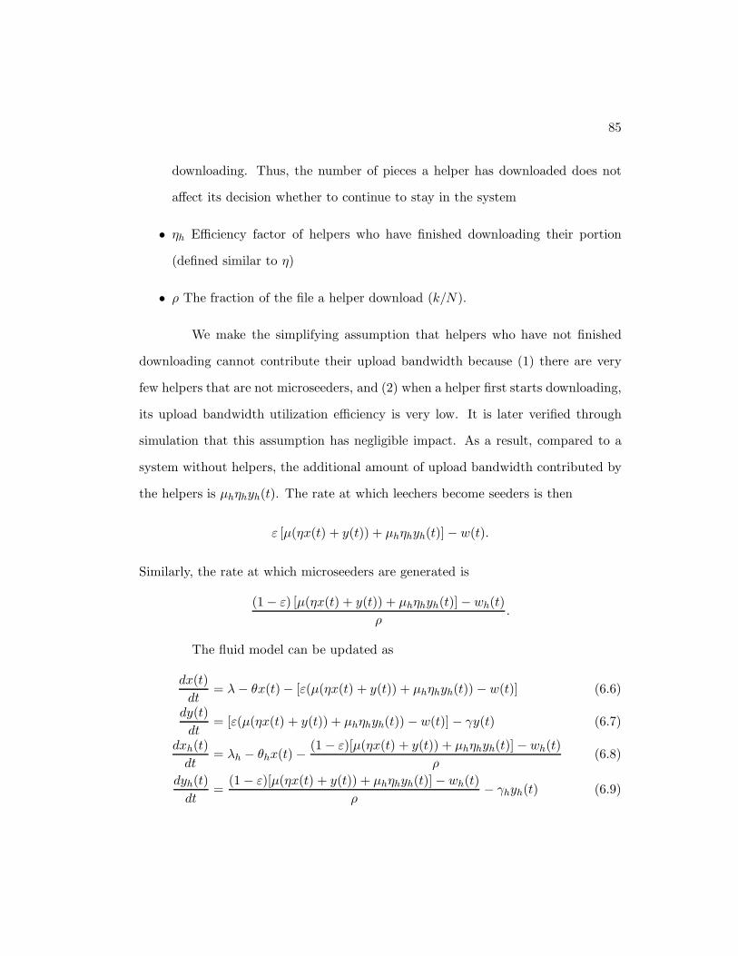
85
downloading. Thus, the number of pieces a helper has downloaded does not
affect its decision whether to continue to stay in the system
• ηh Efficiency factor of helpers who have finished downloading their portion
(defined similar to η)
• ρ The fraction of the file a helper download (k/N).
We make the simplifying assumption that helpers who have not finished
downloading cannot contribute their upload bandwidth because (1) there are very
few helpers that are not microseeders, and (2) when a helper first starts downloading,
its upload bandwidth utilization efficiency is very low. It is later verified through
simulation that this assumption has negligible impact. As a result, compared to a
system without helpers, the additional amount of upload bandwidth contributed by
the helpers is µhηhyh(t). The rate at which leechers become seeders is then
ε [µ(ηx(t) + y(t)) + µhηhyh(t)] − w(t).
Similarly, the rate at which microseeders are generated is
(1 − ε) [µ(ηx(t) + y(t)) + µhηhyh(t)] − wh(t)
ρ.
The fluid model can be updated as
dx(t)
dt= λ − θx(t)− [ε(µ(ηx(t) + y(t)) + µhηhyh(t)) − w(t)] (6.6)
dy(t)
dt= [ε(µ(ηx(t) + y(t)) + µhηhyh(t)) − w(t)] − γy(t) (6.7)
dxh(t)
dt= λh − θhx(t) −
(1 − ε)[µ(ηx(t) + y(t)) + µhηhyh(t)] − wh(t)
ρ(6.8)
dyh(t)
dt=
(1 − ε)[µ(ηx(t) + y(t)) + µhηhyh(t)] − wh(t)
ρ− γhyh(t) (6.9)

86
Again, to study the steady-state behavior, we set (6.6) – (6.9) to zero and
solve for the steady-state average number of peers (x), seeders (y), helpers (xh), and
microseeders (yh) numerically. The download time is now given by
Tdl =1
ε[µ(ηx+y)+µhηhyh]x
. (6.10)
In the next section we show numerical solutions obtained from this analysis
for different simulation setups along with results that demonstrate the accuracy of
the first-order fluid-model analysis.
6.2.4 Evaluations
We have implemented a discrete-time packet-level simulator to simulate a
BitTorrent file sharing system. In this system, leechers follow the BitTorrent pro-
tocol exactly and helpers follow the proposed helper protocol, which is backwards-
compatible with the BitTorrent protocol. Among other things, the simulator ex-
plicitly implements the most important features of the file sharing system/protocol,
namely:
• Accounting for individual pieces of a file;
• Accounting for peer activities such as arrivals, aborts, departures, piece uploads
and piece downloads;
• Local-rarest-first piece selection;
• Tit-for-tat policy in conjunction with choking/unchoking (including optimistic
unchoking);
• Accounting for bandwidths of network links.

87
We first study the accuracy of the fluid model by comparing the average
download time computed using the fluid model to that obtained from simulations.
We use two different setups. Setup 1 mimics a relatively small file with a small-sized
swarm while Setup 2 has a large file with a medium-sized swarm. The parameters
for the 2 setups are shown in Table 6.1. Under each setup, we simulated the system
with and without helpers.
Setup 1 Setup 2
λ(peer/s) 0.2 0.2
θ(1/s) 0.000625 0.0000625
µ(Kbps) 512 512
c(Kbps) 2048 2048
γ(1/s) 0.0025 0.00025
λh(peer/s) 0.05 0.1
θh(1/s) 0.00125 0.00025
µh(Kbps) 512 512
ch(Kbps) 2048 2048
file size (MB) 100 1000(N = 400 pieces) (N = 1000 pieces)
k 8 10
Table 6.1: Parameters of 2 different setups for helper-assisted BitTorrent-compatiblepeer-to-peer file download.
Table 6.2 shows that under both setups, whether there are helpers or not,
the average download time, the number of leechers, and the number of seeders in the
system in steady state are all accurately estimated by the fluid model.
The fact that the fluid-model analysis results closely match the simulation
results has the following implications. First, the assumption that peers’ upload band-
widths are fulled utilized is valid. Indeed, Figure 6.1 plots the system throughput
and the total amount of upload bandwidth in the system under Setup 1. We can see
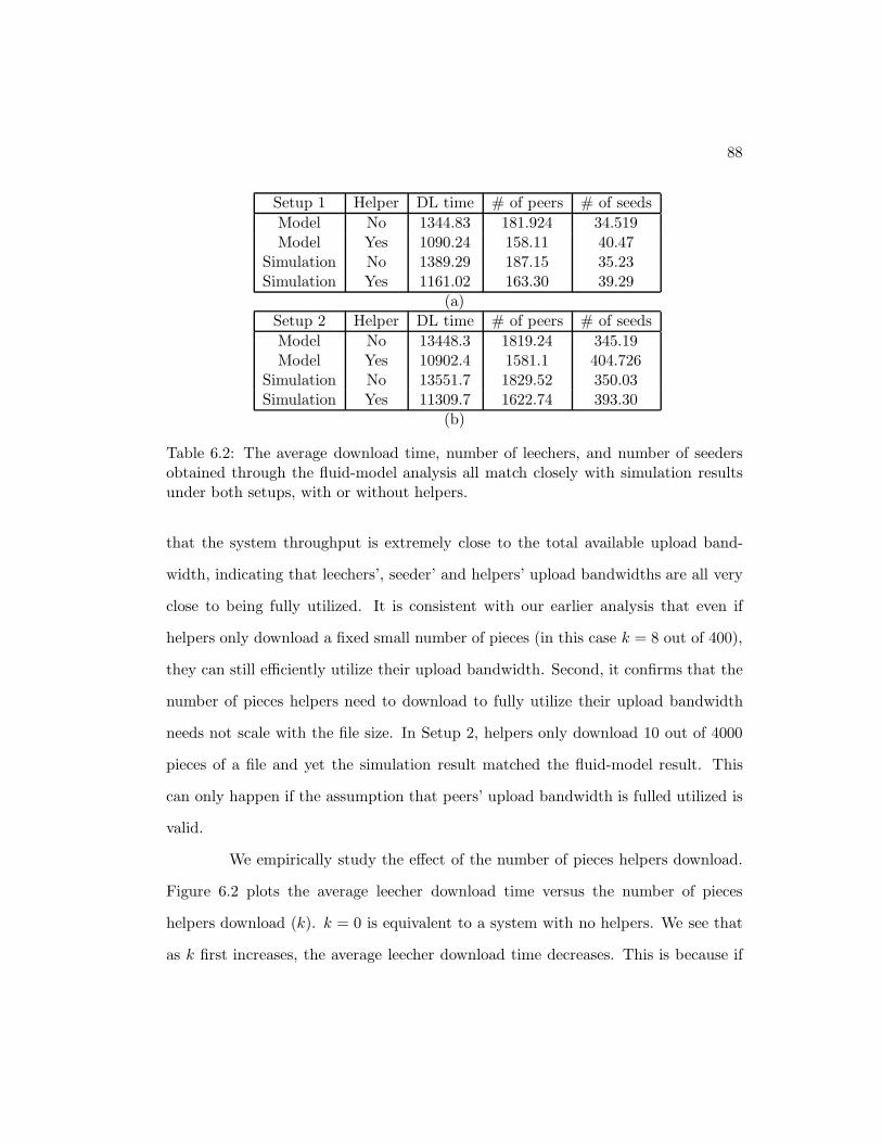
88
Setup 1 Helper DL time # of peers # of seeds
Model No 1344.83 181.924 34.519Model Yes 1090.24 158.11 40.47
Simulation No 1389.29 187.15 35.23Simulation Yes 1161.02 163.30 39.29
(a)
Setup 2 Helper DL time # of peers # of seeds
Model No 13448.3 1819.24 345.19Model Yes 10902.4 1581.1 404.726
Simulation No 13551.7 1829.52 350.03Simulation Yes 11309.7 1622.74 393.30
(b)
Table 6.2: The average download time, number of leechers, and number of seedersobtained through the fluid-model analysis all match closely with simulation resultsunder both setups, with or without helpers.
that the system throughput is extremely close to the total available upload band-
width, indicating that leechers’, seeder’ and helpers’ upload bandwidths are all very
close to being fully utilized. It is consistent with our earlier analysis that even if
helpers only download a fixed small number of pieces (in this case k = 8 out of 400),
they can still efficiently utilize their upload bandwidth. Second, it confirms that the
number of pieces helpers need to download to fully utilize their upload bandwidth
needs not scale with the file size. In Setup 2, helpers only download 10 out of 4000
pieces of a file and yet the simulation result matched the fluid-model result. This
can only happen if the assumption that peers’ upload bandwidth is fulled utilized is
valid.
We empirically study the effect of the number of pieces helpers download.
Figure 6.2 plots the average leecher download time versus the number of pieces
helpers download (k). k = 0 is equivalent to a system with no helpers. We see that
as k first increases, the average leecher download time decreases. This is because if
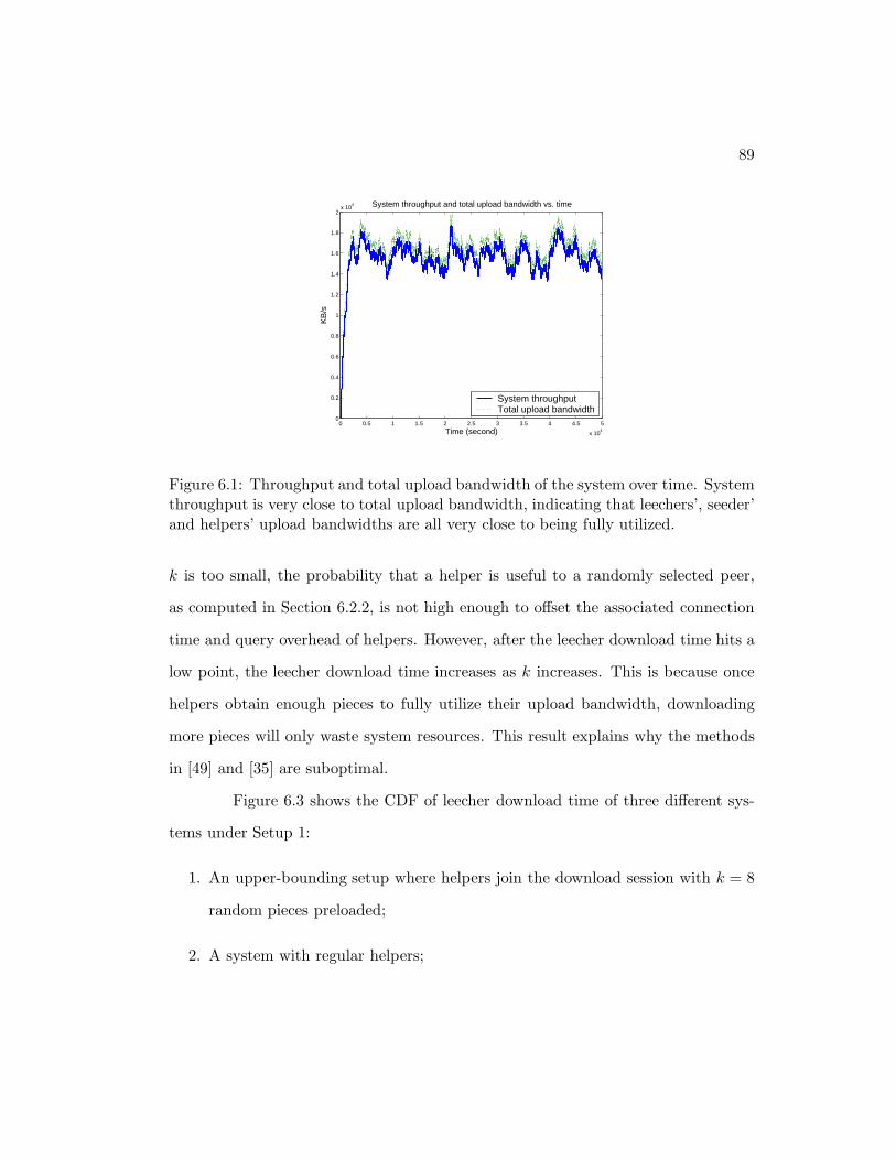
89
0 0.5 1 1.5 2 2.5 3 3.5 4 4.5 5
x 104
0
0.2
0.4
0.6
0.8
1
1.2
1.4
1.6
1.8
2x 10
4
Time (second)
KB
/s
System throughput and total upload bandwidth vs. time
System throughputTotal upload bandwidth
Figure 6.1: Throughput and total upload bandwidth of the system over time. Systemthroughput is very close to total upload bandwidth, indicating that leechers’, seeder’and helpers’ upload bandwidths are all very close to being fully utilized.
k is too small, the probability that a helper is useful to a randomly selected peer,
as computed in Section 6.2.2, is not high enough to offset the associated connection
time and query overhead of helpers. However, after the leecher download time hits a
low point, the leecher download time increases as k increases. This is because once
helpers obtain enough pieces to fully utilize their upload bandwidth, downloading
more pieces will only waste system resources. This result explains why the methods
in [49] and [35] are suboptimal.
Figure 6.3 shows the CDF of leecher download time of three different sys-
tems under Setup 1:
1. An upper-bounding setup where helpers join the download session with k = 8
random pieces preloaded;
2. A system with regular helpers;
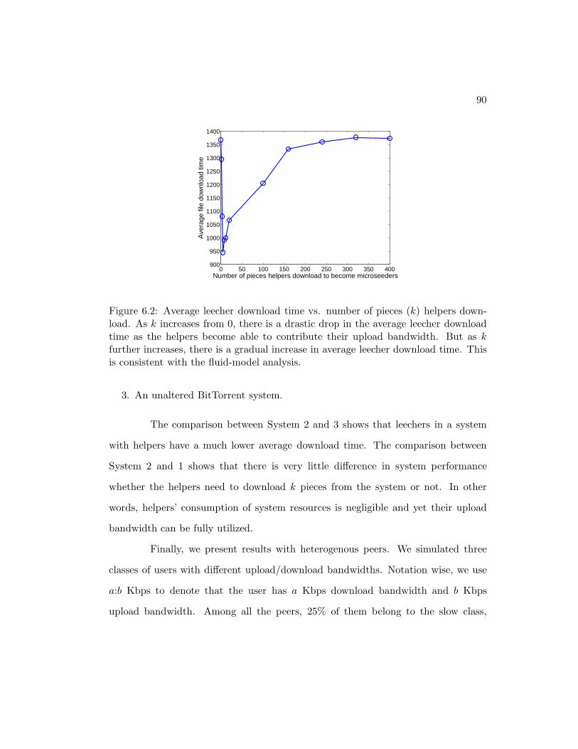
90
0 50 100 150 200 250 300 350 400900
950
1000
1050
1100
1150
1200
1250
1300
1350
1400
Number of pieces helpers download to become microseeders
Ave
rage
file
dow
nloa
d tim
e
Figure 6.2: Average leecher download time vs. number of pieces (k) helpers down-load. As k increases from 0, there is a drastic drop in the average leecher downloadtime as the helpers become able to contribute their upload bandwidth. But as kfurther increases, there is a gradual increase in average leecher download time. Thisis consistent with the fluid-model analysis.
3. An unaltered BitTorrent system.
The comparison between System 2 and 3 shows that leechers in a system
with helpers have a much lower average download time. The comparison between
System 2 and 1 shows that there is very little difference in system performance
whether the helpers need to download k pieces from the system or not. In other
words, helpers’ consumption of system resources is negligible and yet their upload
bandwidth can be fully utilized.
Finally, we present results with heterogenous peers. We simulated three
classes of users with different upload/download bandwidths. Notation wise, we use
a:b Kbps to denote that the user has a Kbps download bandwidth and b Kbps
upload bandwidth. Among all the peers, 25% of them belong to the slow class,
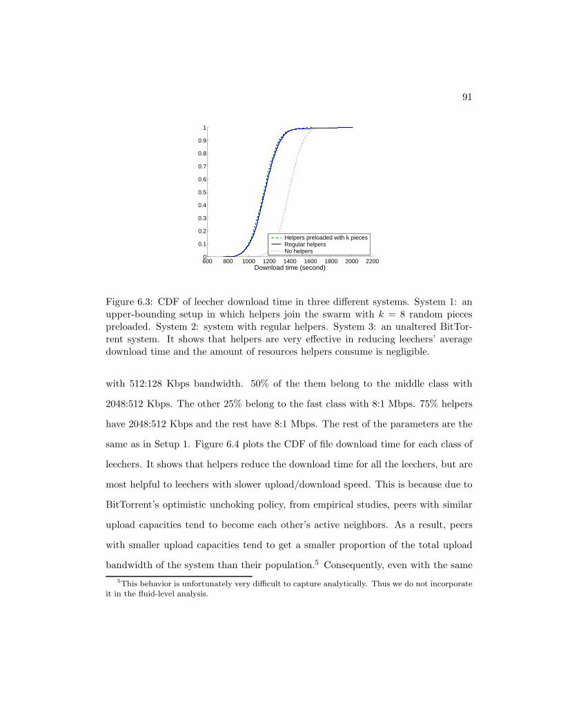
91
600 800 1000 1200 1400 1600 1800 2000 22000
0.1
0.2
0.3
0.4
0.5
0.6
0.7
0.8
0.9
1
Download time (second)
Helpers preloaded with k piecesRegular helpersNo helpers
Figure 6.3: CDF of leecher download time in three different systems. System 1: anupper-bounding setup in which helpers join the swarm with k = 8 random piecespreloaded. System 2: system with regular helpers. System 3: an unaltered BitTor-rent system. It shows that helpers are very effective in reducing leechers’ averagedownload time and the amount of resources helpers consume is negligible.
with 512:128 Kbps bandwidth. 50% of the them belong to the middle class with
2048:512 Kbps. The other 25% belong to the fast class with 8:1 Mbps. 75% helpers
have 2048:512 Kbps and the rest have 8:1 Mbps. The rest of the parameters are the
same as in Setup 1. Figure 6.4 plots the CDF of file download time for each class of
leechers. It shows that helpers reduce the download time for all the leechers, but are
most helpful to leechers with slower upload/download speed. This is because due to
BitTorrent’s optimistic unchoking policy, from empirical studies, peers with similar
upload capacities tend to become each other’s active neighbors. As a result, peers
with smaller upload capacities tend to get a smaller proportion of the total upload
bandwidth of the system than their population.5 Consequently, even with the same
5This behavior is unfortunately very difficult to capture analytically. Thus we do not incorporateit in the fluid-level analysis.
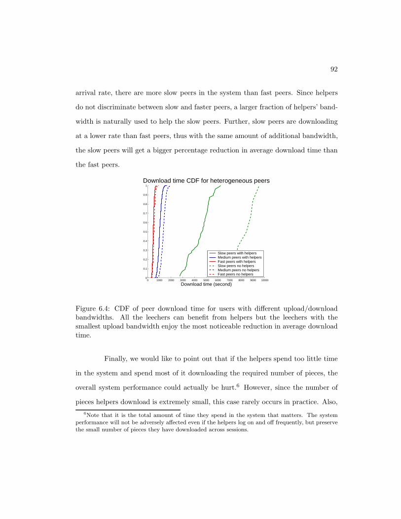
92
arrival rate, there are more slow peers in the system than fast peers. Since helpers
do not discriminate between slow and faster peers, a larger fraction of helpers’ band-
width is naturally used to help the slow peers. Further, slow peers are downloading
at a lower rate than fast peers, thus with the same amount of additional bandwidth,
the slow peers will get a bigger percentage reduction in average download time than
the fast peers.
0 1000 2000 3000 4000 5000 6000 7000 8000 9000 100000
0.1
0.2
0.3
0.4
0.5
0.6
0.7
0.8
0.9
1
Download time (second)
Download time CDF for heterogeneous peers
Slow peers with helpersMedium peers with helpersFast peers with helpersSlow peers no helpersMedium peers no helpersFast peers no helpers
Figure 6.4: CDF of peer download time for users with different upload/downloadbandwidths. All the leechers can benefit from helpers but the leechers with thesmallest upload bandwidth enjoy the most noticeable reduction in average downloadtime.
Finally, we would like to point out that if the helpers spend too little time
in the system and spend most of it downloading the required number of pieces, the
overall system performance could actually be hurt.6 However, since the number of
pieces helpers download is extremely small, this case rarely occurs in practice. Also,
6Note that it is the total amount of time they spend in the system that matters. The systemperformance will not be adversely affected even if the helpers log on and off frequently, but preservethe small number of pieces they have downloaded across sessions.
93
when there are enough helpers in the system to fill up leechers’ download pipes, any
more helpers will not help with system performance. Thus the tracker may use the
fluid model analysis as a guideline to turn away helpers when the helper arrival rate
exceeds the rate required to fill up leechers’ download pipes.
6.3 Extension to live video multicast
In this section, we extend the usage of helpers to a different but impor-
tant class of video distribution: live multicast. Examples include TV-over-Internet
and live sports broadcast. Compared to file download, live video multicast has the
following defining characteristics:
1. Peers in the system have synchronized playback time;
2. Each packet has a specific delivery deadline;
3. The streaming content is constantly updated.
These characteristics make efficient utilization of helpers even more crucial. As
the streaming content constantly changes, helpers must be constantly downloading
in order to be constantly uploading. Like in the download case, helpers have to
upload more than they download to contribute to the system. Further, helpers must
distribute packets to meet specific delivery deadlines.
We consider a hybrid system in which the content server will supplement
the extra bandwidth that peers are not able to obtain from each other. The main
performance metric of such a system is the required server bandwidth given the
same startup delay and buffer length. In such a system, if the video bit rate is

94
lower than the average peer upload bandwidth, the system can be maintained with
very little server bandwidth [32, 41]. However, if that is not the case, the server
bandwidth will increase linearly with the number of peers in the system, which is
not scalable. Our goal is to optimally utilize helpers’ upload capacity in order to
provide video streaming at rate beyond peers’ average upload bandwidth without
incurring additional server load.
6.3.1 Design guideline
One equivalent way of formulating our problem is to maximize peers’ stream-
ing rate R given a fixed set of peers, helpers, and server load. We use a first-order
fluid-level analysis to guide the system design. Recall that in Section 6.2.3, we also
use a fluid-level analysis and establish equations regarding the rates at which the
numbers of each type of peers change. Here we take a snapshot of the system and
use the following simple relationship to derive a performance upper bound. At any
point of time,
total system upload bandwidth ≥ sum of peers’ downloading rate.
Let P and H denote the set of peers and helpers in the system respectively.
|P | and |H| are the numbers of peers and helpers respectively. Let ui be the upload
bandwidth of Peer i and uHj be the upload bandwidth of Helper j. Let SP and SH
denote the fixed total bandwidth server allocates to peers and helpers respectively.
Let RP→P denote the total traffic among peers and RH→H denote the total traffic
among helpers. Similarly, let RP→H denote the total traffic from peers to helpers and
RH→P denote the total traffic from helpers to peers. RHi denotes the rate Helper i
receives.
95
The total rates that peers and helpers receive are
|P |R = SP + RP→P + RH→P , and (6.11)
∑
i∈H
RHi = SH + RH→H + RP→H respectively. (6.12)
The system throughput has to be smaller than or equal to the total available
upload bandwidth. Therefore
RH→H + RP→H + RP→P + RH→P ≤∑
i∈P
ui +∑
i∈H
uHi . (6.13)
Combining (6.11), (6.12) and (6.13) yields
R ≤SH + SP +
∑
i∈P ui +∑
i∈H uHi −
∑
i∈H RHi
|P |. (6.14)
To maximize R, we need to minimize∑
i∈H RHi while keeping both peers
and helpers fully utilizing their upload capacity. In practice, RHi cannot be made
arbitrarily small for two reasons. Firstly, video data is broken into packets and
transmitted. The packets cannot be too small in size in order to reduce transmission
overhead. Let us conceptualize video as being broken into short segments, each m
seconds long. Each segment consists of k packets of equal sizes. Then for a helper
to be useful to peers downloading a particular segment, the least it has to download
is one packet. As peers move forward in playback time constantly, helpers have to
download at least 1 packet out of every segment (k packets). Therefore, RHi ≥ R
k
and∑
i∈H RHi ≥ |H|R
k. Secondly, RH
i caps the rate at which Helper i can upload
to any one peer. Thus, for Helper i to fully utilize its upload bandwidth, it has to
constantly haveuH
i
RHi
peers to upload to, which cannot be maintained if RHi is too
small.
96
To summarize, we have
R ≤SH + SP +
∑
i∈P ui +∑
i∈H uHi
|P | + |H|k
, (6.15)
where equality holds if each helper downloads only 1 packet out of every k packets of
a segment, and all the peers and helpers in the system can fully utilize their upload
bandwidth.
While it has been shown in previous works, e.g. [33, 53], that peers can
very efficiently utilize their upload bandwidth in video streaming over P2P overlay
networks, we need helpers to also fully utilize their upload bandwidth even if they
only have 1 packet out of every k packet. In a highly dynamic environment, if each
helper carries one random uncoded data packet for each segment, it can be difficult for
helpers to be consistently connected to enough peers that are missing the particular
packets they are carrying, especially for unstructured overlay networks. As a result,
helpers either have unused upload bandwidth or waste a lot of resources establishing
connections. Instead, we propose a system in which peer helper carries one MDS
erasure coded packet of each segment. Figure 6.5 illustrates the proposed solution.
The content server breaks each segment of video into k packets and generates n − k
parity packets using an (n, k) systematic MDS erasure code. The server uploads the
k data packets to the peers at rate SP ≥ R. Helpers break into n − k clusters with
approximately the same total upload bandwidth. Every m seconds (the length of a
segment), the server uploads 1 unique parity packet to each helper cluster at total
rate SH = R(n−k)k
. Each cluster of helpers circulate among themselves one and only
one parity packet, i.e. RHj = R
k, ∀j. Each peer maintains connection to each cluster
and requests parity packets when needed.
If the average upload bandwidth of peers is∑
i∈P ui
|P | = αR (α < 1), then on
97
average, peers miss (1−α)k packets out of every k packets of a segment. This requires
that the helpers have at least αk unique parity packets, i.e. n − k ≥ αk =k∑
i∈P ui
|P | .
Peers can miss at most k packets in each segment therefore n−k ≤ k. However, since
SH does not scale with the number of helpers or the number of peers, it is beneficial
to pick n − k = k such that the helper clusters can potentially accommodate the
entire packet drop range.
In addition to ease of finding peers to upload to, there are other benefits
to having helpers carry parity packets instead of random uncoded data packets. De-
pending on the explicit implementation of the P2P overlay and the packet exchange
strategy, there may be particular packets that a lot of peers are missing due to peer
churning or link congestion. It is also difficult to predict which packet(s) will be
in such demand. If the helpers carry uncoded packets, some helpers will be over-
stressed while others will have spare capacity. This effect is mitigated if helpers carry
coded packets. In short, we would like each helper to be equally useful to all peers
to facilitate full utilization of helpers’ upload bandwidth. This is also why we would
like to keep the available upload bandwidth of each helper cluster approximately the
same. We will demonstrate through simulations that the proposed system is one of
the constructive solutions that can approach the equality in (6.15) very closely.
6.3.2 Rate allocation
As stated earlier, for equality to hold in (6.15), we need both peers and
helpers to be fully utilizing their upload bandwidth. In a P2P system, each peer
connects to multiple other peers (neighbors) simultaneously. Compared to download
capacity, peers’ upload capacity is limited and oftentimes the most prominent con-
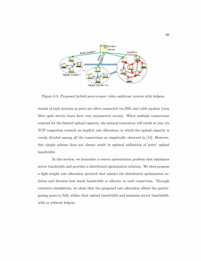
98
Figure 6.5: Proposed hybrid peer-to-peer video multicast system with helpers.
straint of such systems as peers are often connected via DSL and cable modem (even
fiber optic service hosts have very asymmetric access). When multiple connections
contend for the limited upload capacity, the natural contention will result in (say via
TCP congestion control) an implicit rate allocation, in which the upload capacity is
evenly divided among all the connections as empirically observed in [13]. However,
this simple scheme does not always result in optimal utilization of peers’ upload
bandwidth.
In this section, we formulate a convex optimization problem that minimizes
server bandwidth and provides a distributed optimization solution. We then propose
a light-weight rate allocation protocol that mimics the distributed optimization so-
lution and dictates how much bandwidth to allocate to each connection. Through
extensive simulations, we show that the proposed rate allocation allows the partici-
pating peers to fully utilize their upload bandwidth and minimize server bandwidth,
with or without helpers.
99
Notations and assumptions
Suppose there are n peers in the system at any instant of time. Denote
them as Peer k (k = 1, 2, ..., n). When Peer j arrives, it connects to a subset of peers
already in the system (say including Peer i) and requests data from them. xi,j is the
rate Peer i allocates from its upload capacity ui to serve Peer j. Each peer keeps track
of its total upload capacity, which can initially be estimated based on historical values
and then measured/updated once data starts to flow to its neighbors. Nj denotes the
set of all peers connected to Peer j (Peer j’s neighbors). The aggregate rate Peer j
receives from all of its neighbors is denoted as xj =∑
i∈Njxi,j. Denote R as the
video bitrate. R is also Peer j’s desired streaming rate in order to maintain smooth
video playback. It is clear that smooth video playback requires xj ≥= R. If xj < R,
Peer j will request data from the server at rate R − xj to make up for the deficit.
The aggregate rate at which Peer i uploads to all its neighbors is∑
j∈Nixi,j. Clearly,
this cannot exceed Peer i’s upload bandwidth, i.e.,∑
j∈Nixi,j ≤ ui. Furthermore, for
unified representation, we denote the server as Peer 0. Thus, x0,j is the rate Peer j
obtains from the server, which satisfies x0,j = max(0, R − xj).
In the analysis, we assume that a peer (say Peer A) can upload to another
peer (say Peer B) as fast as they want within its upload capacity. In practice, the
speed at which Peer A can upload to Peer B is also determined by how much content
is needed by Peer B from Peer A. This assumption is automatically removed in the
packet-level simulation.
100
Optimization framework
The most straightforward formulation of minimizing the server load using
an optimization framework is the following:
min∑
j
max(0, R −∑
i∈Nj
xi,j) (6.16)
s.t.∑
j∈Ni
xi,j ≤ ui ∀ i 6= 0, and (6.17)
xi,j ≥ 0 ∀ i, j. (6.18)
We introduce a utility function f(·) for each peer in terms of the aggregate
rate received from all its neighbors (excluding the server or Peer 0). We show that if
f(·) is monotonically increasing, differentiable everywhere and strictly concave, the
solution to maximizing the total system utility will also minimize server load. This
optimization problem bears a distributed solution that is suitable for large scale P2P
systems.
Proposition 2. If f(·) is monotonically increasing and strictly concave, solutions
to
max∑
j
f(∑
i∈Nj
xi,j) (6.19)
s.t.∑
j∈Ni
xi,j ≤ ui ∀ i 6= 0, and (6.20)
xi,j ≥ 0 ∀ i, j. (6.21)
are a subset of solutions to (6.16) and hence minimize server load.
Proof. Because f(·) is monotonically increasing, it is easy to show through contra-
diction that when∑
j f(xj) is maximized,∑
j∈Nixi,j = ui ∀ i.
101
Since f(·) is strictly concave in xi,j and monotonically increasing,∑
j∈Nixi,j−
ui is concave in xi,j,∑
j∈Nixi,j = ui ∀ i, the necessary and sufficient conditions for
(6.19) are:
d
dxi,jf(∑
i∈Nj
xi,j) − µi + γi,j = 0 ∀ j, (6.22)
µi > 0 ∀ i, (6.23)
γi,j ≥ 0 ∀ i, j, (6.24)
γi,jxi,j = 0 ∀ i, j. (6.25)
For these necessary and sufficient conditions to be satisfied, for Peer i, either
xi,j = 0, or ddxi,j
f(∑
i∈{0,Nj}xi,j) = µi ∀ j ∈ Ni.
Since (6.16) has the exact same constraints as (6.19), it is easy to show that
any solution that satisfies the necessary and sufficient conditions of (6.19) will also
satisfy the sufficient conditions for (6.16). Hence any solution for (6.19) is also a
solution to (6.16).
Distributed solution
One important characteristic of (6.19) is that the constraints are local in
that the rate assignment xi,j is constrained locally at Peer i, i.e. xi,j ≥ 0 and
∑
j∈Nixi,j ≤ ui. This allows us to use a classical iterative algorithm for convex
optimization and directly obtain a distributed solution to (6.19) [11].
Specifically, we adopt the gradient projection algorithm. At Peer i, xi,j is
initialized to ui
|Ni|for j ∈ Ni and 0 otherwise, where |Ni| is the number of neighbors
Peer i has. xi,j is updated at each step as follows:

102
xi,j = ∆ ·∂
∂xi,jf(∑
i∈Nj
xi,j), (6.26)
xi,j = [xi,j + xi,j]+ (6.27)
where [·]+ denotes l2 projection onto a feasible set.
With the constraints on xi,j, the objective function in (6.19) satisfies Lips-
chitz condition. Thus, by carefully choosing the update step size ∆, convergence can
be guaranteed [11].
Here we propose a light-weight heuristic based protocol that mimics this
optimization solution. The essence of the solution is that Peer i slowly adjusts the
rate at which it uploads to its neighbors such that its neighbors’ aggregate received
bandwidth is the same, i.e. ddxi,j
f(∑
i∈{0,Nj}xi,j) = µi ∀ j ∈ Ni. Since a peer’s buffer
level is a good reflection of its aggregate received bandwidth, we try to equalize each
peer’s neighbors’ buffer levels by having peers upload the next packet to the neighbor
with the lowest buffer level.
We will detail the system description and discuss the complexity of this
protocol in the following section. We will then demonstrate the effectiveness of this
rate allocation scheme in Section 6.3.4.
6.3.3 System description
With these design guidelines in mind, we now present the proposed sys-
tem in detail. Before describing how the helpers function, we first describe the peer
network for the sake of completeness. The peer network we use is an unstructured
mesh-based overlay network similar to [33] and [53]. We choose to use an unstruc-
103
tured overlay to reduce network maintenance overhead, which is essential in high-
churn applications like live video streaming. However, the proposed helper system
will work with a structured tree (or multi-tree) based peer overlay network as well.
Peer network
Overlay network formation and maintenance: The content provider owns a
source node (content server) that connects to a small number of peers (20 in our
case). Similar to BitTorrent, the content provider also maintains another server,
called tracker, to keep track of all the peers in the streaming session and to assist
building the overlay network7. A joining peer first queries the tracker to obtain a list
of peers and synchronize with system clock. It then contacts these peers to establish
connections with them. Each peer is allowed a maximum number of neighbors, which
is proportional to its upload bandwidth. A peer will reject a new connection request
if it already has enough neighbors. If the number of neighbors connected to a peer
falls below a threshold, the peer will contact the tracker to obtain a new list of
peers to connect to. In our implementation, when the tracker is queried for a list of
peers, it chooses randomly among the existing peers. This may result in an inefficient
overlay network. To improve the quality of the network, we adopt a neighbor-pruning
method similar to the one described in [53]. Specifically, each peer periodically (every
5 seconds in our case) checks the throughput between itself and each of its neighbors.
If the throughput is below a certain threshold, it will disconnect from that neighbor.
This method has shown to greatly improve the system throughput of a practical
system [53].
7Tracker can also be distributed using distributed hash table techniques.
104
Peer packet exchange protocol: The source node generates new packets with
monotonically increasing ID’s in real-time. Like in [33], each peer maintains a window
of interest, which is the range of packets that it is interested in obtaining. Each peer
also maintains a window of availability, which is the range of packets that it is
willing to share with its neighbors. Peers exchange packets by updating each other
with availability maps and using a pull-based packet request protocol. We assume
each second of video consists of an integer number of GOPs and k equal sized packets
packets. Peer move both their window of interest and window of availability forward
once every one-second. Note that this interval is correlated with the maximum
startup delay of the system. The longer this interval, the longer the startup delay.
This is because before the peers can slide their windows forward for the first time,
they need to first fill up their window of interest to that amount.
To choose which packet to request from each neighbor, peers follow a
BitTorrent-like local-rarest-first strategy within its window of interest and requests
the packet that is the rarest within its one-hop neighborhood. Naturally, a peer
may have multiple requests pending. In choosing which request to fulfill first, as
discussed in Section 6.3.2, instead of choosing randomly or following a round-robin
fashion, peers first satisfy the request from a neighbor who possesses the fewest num-
ber of packets in its window of interest. Intuitively, this strategy works because a
peer’s upload bandwidth can only be utilized if it has packets that other peers need.
Thus if a peer has too few packets in its buffer, it may not be able to fully utilize its
upload bandwidth. On the other hand, if a peer already has a lot of packets, it most
likely already has a lot of pending requests. Since its upload bandwidth is limited,
it cannot satisfy all these requests even if it gets more packets. Therefore, in terms
105
of increasing system throughput, it isn’t as meaningful to fulfill the request of a peer
that already has a lot of packets.
In the analysis in Section 6.3.2, we assume that Peer i can upload to Peer j
at rate xi,j as long as the upload bandwidth constraint is not violated. In practice, xi,j
cannot be realized unless Peer i has sufficient content that Peer j needs. Therefore we
build the topology such that peers with more upload bandwidth have more neighbors.
Given the same number of packets in the buffer, peers with more upload bandwidth
get more packet requests and can thus still fully utilize their upload bandwidth. This
greatly reduces the need to have a sophisticated algorithm that also takes peers’
upload bandwidth into consideration. The information regarding the fullness of a
peer’s window of interest can be easily piggy-backed in the packet request with
marginal overhead.
Like in [33], the content server also implements request overriding at the
source. Specifically, the content source, or server, maintains a list of packets that
have never been uploaded before. If the list is not empty and the server receives a
request for a packet that is not on the list, the server will ignore the packet request,
send the oldest packet on the list instead, and delete that packet from the list. This
algorithm ensures that at least one copy of every packet is uploaded quickly, and
the server will not spend its upload bandwidth on uploading packets that could be
obtained from other peers unless it has spare bandwidth available.
As we show shortly in the Section 6.3.4, the resulting video streaming over-
lay network is quite efficient, utilizing more than 97% of peers’ available bandwidth.
106
Helper network
As mentioned earlier, the rate that the content server allocates helpers is
SH = R(n−k)k
, which does not scale with the number of helpers or peers. Thus, we
choose n = 2k. The content owner applies a (2k, k) systematic MDS erasure code
over each second of video data and generate k distinct parity packets for the k helper
clusters. Ideally, we would like each of the helper cluster to have the same amount
of spare upload bandwidth. To approximate this, the tracker keeps track of the
total amount of upload bandwidth of each helper cluster. As a new helper joins the
network, it reports to trackers its estimated upload bandwidth. The tracker then
assigns it to the helper cluster with the least amount of available upload bandwidth.
For instance, let Helper i have upload bandwidth ui. The amount of bandwidth it
can contribute to the system is then ui − R/k. If a cluster has N helpers, the total
available upload bandwidth is then (∑i=N
i=1 ui) −NRk
. In practice, helpers’ upload
bandwidth may fluctuate and they can update the tracker when needed.
Each cluster of helpers will form their own overlay network and exchange
packets with each other using the exact same mechanism as regular peers. To further
facilitate full utilization helpers’ upload bandwidth, we have the helpers download
content 1 second ahead of peers. For example, if the current time is 14 second and
the buffer length is 5 second, then the peers share data packets up to the 9th second
and the helpers share parity packets up to the 10th second. This way, peers can
download from helpers without having to wait for them to finish downloading the
parities first.
107
Interaction between peers and helpers
As a peer joins, it also queries the tracker for a list of helpers. Each peer
maintains connections to at least one helper from each of the n − k = k clusters.
Each helper is allowed a maximum number of peer neighbors that is proportional
to its upload bandwidth. Peers periodically prune helpers that consistently fail to
provide the requested packets in time.
Helpers inform all their neighbors (both peers and helpers) every time they
receive a new packet. As they receive only one new packet per second on average,
the overhead is small.
In deciding what to request from helpers, peers partition their window
of interest into two parts: urgent and regular. The urgent part of the buffer is
the part that is close to being shifted out of the downloading buffer for processing
and playback. Suppose it is of length u second. A peer will always request parity
packets for the urgent part first if it has not started receiving uk distinct packets
in that interval. It will also flag the request control message as urgent. For the
regular buffer zone, peers request parity packets in a local-rarest-first manner. In
our implementation, the urgent zone is one second long. In general, the urgent zone
length can be any integer multiple of the window-sliding interval.
Helpers use the following rules to decide which request to satisfy first.
Helpers will always satisfy requests from other helpers first, as this will enable other
helpers to contribute their upload bandwidth. Among peers’ requests, helpers will
always satisfy the urgent requests first. For the regular requests from peers, helpers
will first satisfy the peers whose buffer levels are the lowest to mimic the distributed
optimization solution.
108
6.3.4 Simulation results
We evaluate the performance of the proposed system through a discrete-
time packet-level simulator. The simulator implements the most important compo-
nents of the system including: (i) accounting for individual packets of video data
(we use n = 40, k = 20 per second of video.); (ii) peer activities such as arrivals,
departures, packet uploads and downloads; (iii) packet request algorithm; (iv) over-
lay network maintenance and (v) bandwidth constraints of peers. The downloading
buffer keeps 10 seconds’ data and the startup delay is 3 seconds.8 All the tests are
500 seconds long.
We first present simulation results with non-churning heterogeneous peers
to demonstrate that both peers’ and helpers’ upload bandwidth can be efficiently
utilized using the proposed system and the number of helpers needed can be rea-
sonably estimated using the simple computation in (6.15). All the peers (including
helpers) have unlimited download bandwidth and the following upload bandwidth
distribution: 40% of them have 384 Kbps upload bandwidth, 40% have 512 Kbps and
the other 20% have 768 Kbps. The average upload bandwidth of peers is 512 Kbps.
The number of peers in the system is 2000. Peers enter the system at Time 0 and
stay until the end, as do helpers. We plot the bandwidth needed from the server as
a percentage of total bandwidth consumed by peers watching the video. The dashed
line is the result computed from the simple fluid-level analysis whereas the solid line
was obtained through simulation. When there are no helpers in the system, the
bandwidth shortage is just slightly above 20%. This is expected since peers’ average
upload bandwidth is 20% less than video bitrate. This also indicates the peer net-
8Upon joining, video will start playing after exactly 3 seconds. Peers fetch from the server ifneeded to start playing by the end of 3 seconds.
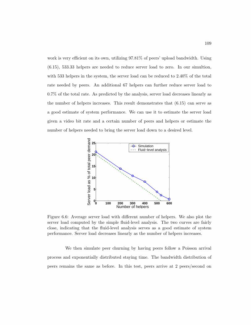
109
work is very efficient on its own, utilizing 97.81% of peers’ upload bandwidth. Using
(6.15), 533.33 helpers are needed to reduce server load to zero. In our simultion,
with 533 helpers in the system, the server load can be reduced to 2.40% of the total
rate needed by peers. An additional 67 helpers can further reduce server load to
0.7% of the total rate. As predicted by the analysis, server load decreases linearly as
the number of helpers increases. This result demonstrates that (6.15) can serve as
a good estimate of system performance. We can use it to estimate the server load
given a video bit rate and a certain number of peers and helpers or estimate the
number of helpers needed to bring the server load down to a desired level.
0 100 200 300 400 500 6000
5
10
15
20
25
Ser
ver
load
as
% o
f tot
al p
eer
dem
and
Number of helpers
SimulationFluid−level analysis
Figure 6.6: Average server load with different number of helpers. We also plot theserver load computed by the simple fluid-level analysis. The two curves are fairlyclose, indicating that the fluid-level analysis serves as a good estimate of systemperformance. Server load decreases linearly as the number of helpers increases.
We then simulate peer churning by having peers follow a Poisson arrival
process and exponentially distributed staying time. The bandwidth distribution of
peers remains the same as before. In this test, peers arrive at 2 peers/second on
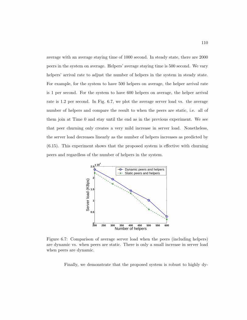
110
average with an average staying time of 1000 second. In steady state, there are 2000
peers in the system on average. Helpers’ average staying time is 500 second. We vary
helpers’ arrival rate to adjust the number of helpers in the system in steady state.
For example, for the system to have 500 helpers on average, the helper arrival rate
is 1 per second. For the system to have 600 helpers on average, the helper arrival
rate is 1.2 per second. In Fig. 6.7, we plot the average server load vs. the average
number of helpers and compare the result to when the peers are static, i.e. all of
them join at Time 0 and stay until the end as in the previous experiment. We see
that peer churning only creates a very mild increase in server load. Nonetheless,
the server load decreases linearly as the number of helpers increases as predicted by
(6.15). This experiment shows that the proposed system is effective with churning
peers and regardless of the number of helpers in the system.
200 250 300 350 400 450 500 550 6000
0.5
1
1.5
2
2.5x 10
4
Ser
ver
load
(K
Bps
)
Number of helpers
Dynamic peers and helpersStatic peers and helpers
Figure 6.7: Comparison of average server load when the peers (including helpers)are dynamic vs. when peers are static. There is only a small increase in server loadwhen peers are dynamic.
Finally, we demonstrate that the proposed system is robust to highly dy-
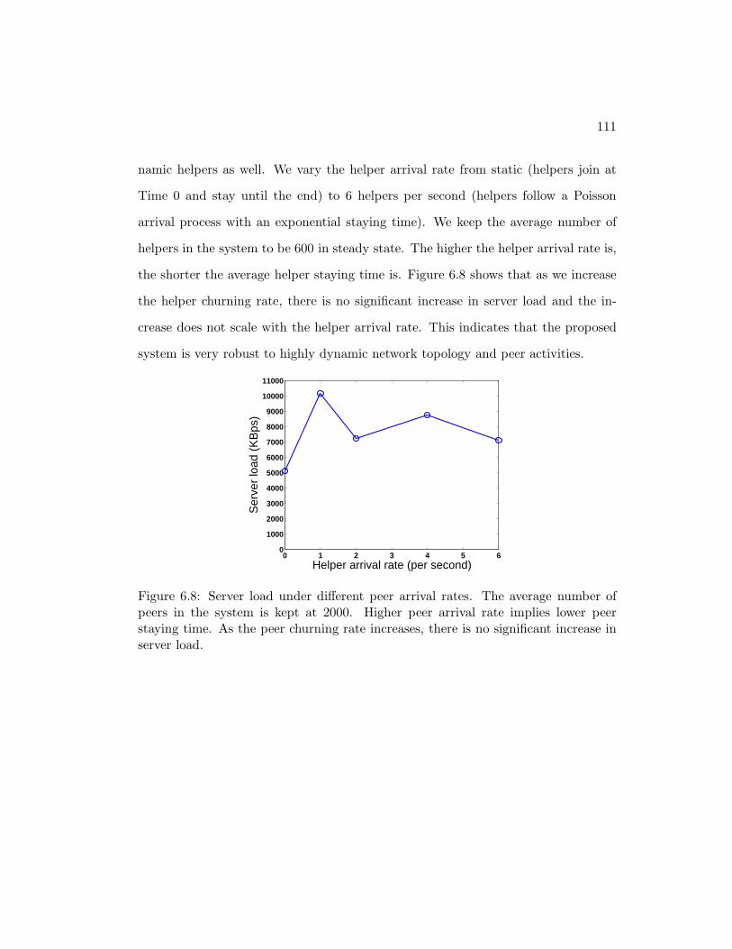
111
namic helpers as well. We vary the helper arrival rate from static (helpers join at
Time 0 and stay until the end) to 6 helpers per second (helpers follow a Poisson
arrival process with an exponential staying time). We keep the average number of
helpers in the system to be 600 in steady state. The higher the helper arrival rate is,
the shorter the average helper staying time is. Figure 6.8 shows that as we increase
the helper churning rate, there is no significant increase in server load and the in-
crease does not scale with the helper arrival rate. This indicates that the proposed
system is very robust to highly dynamic network topology and peer activities.
0 1 2 3 4 5 60
1000
2000
3000
4000
5000
6000
7000
8000
9000
10000
11000
Ser
ver
load
(K
Bps
)
Helper arrival rate (per second)
Figure 6.8: Server load under different peer arrival rates. The average number ofpeers in the system is kept at 2000. Higher peer arrival rate implies lower peerstaying time. As the peer churning rate increases, there is no significant increase inserver load.
112
Chapter 7
Conclusion and future work
In this part of the thesis, we studied enhancing performance of video distri-
bution over uplink-scarce peer-to-peer networks by optimally utilizing helper peers’
upload bandwidths. It is important to understand that higher system throughput
does not necessarily lead to better system performance. This is because while helpers
can increase system throughput by contributing their upload bandwidth, they also
need to consume system resource before they become useful. We have developed
light-weight and distributed helper protocols for both video file download and live
multicast such that helpers can maximally contribute their upload bandwidth while
minimally consuming system resources. We have analyzed system performances us-
ing first-order analysis and cross-verified through extensive simulations. Our simula-
tion results demonstrate that helpers can indeed almost fully contribute their upload
bandwidth and improve system performances.
Along this line of work, there are numerous promising directions for future
research.

113
• For file download, it would be interesting to analyze system performance under
arbitrary peer arrival and departure processes.
• We would like to extend the usage of helper to video-on-demand streaming.
While there exist simple strategies that work well, finding the optimal usage
of helpers is challenging due to the unique attributes of asynchronous play-
back times and the possibility of downloading ahead of playback point in VoD
systems.
• Optimal usage of helpers across different P2P sessions is an interesting topic.
Specifically, we are interested in developing a distributed solution. The goal is
to have helpers independently determine which session or sessions or join with
minimal interaction with central servers.
• Incentive, especially incentive with shared memory, for all P2P systems remains
an active area of research and an open question in general.
We believe the P2P framework is a useful tool to enable high-quality In-
ternet video that can scale gracefully to millions of viewers. In this thesis, we have
only touched a tip of the iceberg. We hope the philosophy of this work can provided
some ideas and intuitions to researchers in this area.
114
Bibliography
[1] [Online]. Available: http://dss.clip2.com/GnutellaProtocol04.pdf
[2] “KaZaA.” [Online]. Available: http://www.kazaa.com
[3] “SETI@home.” [Online]. Available: http://setiathome.ssl.berkeley.edu/
[4] “Skype.” [Online]. Available: http://www.skype.com
[5] “Global Internet Geography 2006,” TeleGeography Research, 2006.
[6] A. Amraoui and R. Urbanke, “Ldpcopt,” 2003. [Online]. Available:http://lthcwww.epfl.ch/research/ldpcopt/bschelp.php
[7] X. Artigas, J. Ascenso, M. Dalai, S. Klomp, D. Kubasov, and M. Ouaret, “TheDISCOVER Codec: Architecture, Techniques and Evaluation,” Proc. PictureCoding Symposium, 2007.
[8] A. Ashikhmin, G. Kramer, and S. Brink, “Extrinsic information transfer func-tions: model and erasure channel properties,” IEEE Trans. Information Theory,vol. 50, pp. 2657–2673, Nov 2004.
[9] S. Battista, F. Casalino, and C. Lande, “MPEG-4: A Multimedia Standard forthe Third Millennium. 1,” IEEE Multimedia, October-December 1999.
[10] ——, “MPEG-4: A Multimedia Standard for the Third Millennium. 2,” IEEEMultimedia, January-March 2000.
[11] D. Bertsekas and J. Tsitsiklis, Parallel and Distributed Computation. OldTappan, NJ (USA); Prentice Hall Inc., 1989.
[12] N.-M. Cheung and A. Ortega, “Compression Algorithms for Flexible Video De-coding,” in Proceedings of Visual Communications and Image Processing, Jan.2008.
115
[13] D. Choffnes and F. Bsutamante, “Taming the Torrent: A Practical Approachto Reducing Cross-ISP Traffic in Peer-to-Peer Systems,” in Proceedings of ACMSIGCOMM, 2008.
[14] B. Cohen, “Incentives build robustness in BitTorrent,” Proceedings of Workshopon Economics of Peer-to-Peer Systems, 2003.
[15] G. Cote, B. Erol, M. Gallant, and F. Kossentini, “H.263+: Video Coding atLow Bit Rates,” IEEE Trans. on Circuits and Systems for Video Technology,1998.
[16] T. M. Cover and J. A. Thomas, Elements of Information Theory. New York:John Wiley and Sons, 1991.
[17] G. Daily, “MSNBC makes mess of democratic debate webcast,” StreamingMe-dia.com, Feb 2008.
[18] S. Draper and E. Martinian, “Compound conditional source coding, Slepian-Wolf list decoding, and applications to media coding,” Proc. International Sym-posium on Information Theory, 2007.
[19] G. D. Forney, “Coset Codes-Part I: Introduction and Geometrical Classifica-tion,” IEEE Trans. on Information Theory, 1988.
[20] ——, “Coset Codes-Part II: Binary Lattices and Related Codes,” IEEE Trans.on Information Theory, 1988.
[21] B. Girod, A. Aaron, S. Rane, and D. Rebollo-Monedero, “Distributed videocoding,” in Proceedings of the IEEE, 2005.
[22] M. Goodman, “2007 Internet Video Forecast: Moving Beyond YouTube,” Yan-kee group, 2007.
[23] C. Guillemot, F. Pereira, L. Torres, T. Ebrahimi, R. Leonardi, and J. Oster-mann, “Distributed Monoview and Multiview Video Coding: Basics, Problemsand Recent Advances,” IEEE Signal Processing Magazine, 2007.
[24] L. Guo, S. Chen, Z. Xiao, E. Tan, X. Ding, and X. Zhang, “Measurements, anal-ysis and modeling of bittorrent-like systems,” in Proceedings of ACM InternetMeasurement Conference, Oct. 2005.
[25] B. G. Haskell, A. Puri, and A. N. Netravali, Digital Video: An Introduction toMPEG-2. Kluwer Academic Publishers, 1996.
116
[26] D. Kaplan, “Oprah web show crashes on huge audience,” New York Post, Mar.2008.
[27] L. Liang, P. Salama, and E. Delp, “Unequal error protection using Wyner-Zivcoding for error resilience,” Proc. Visual Communications and Image Processing,2007.
[28] S. Lin, D. Costello, and M. Miller, “Automatic-repeat-request error-controlschemes,” IEEE Communications Magazine, vol. 22.
[29] F. J. Macwilliams and N. J. A. Sloane, The Theory of Error Correcting Codes.Elseiver-North-Holland, 1977.
[30] S. McCanne, V. Jacobson, and M. Vetterli, “Receiver-driven layered multicast,”in Proceedings of ACM SIGCOMM, Aug. 1996.
[31] W. Norton, “Internet video: the next wave of massive disruption to the U.S.peering ecosystem,” Clean Slate Networking Research Workshop, 2007.
[32] V. Padmanabhan, H. Wang, P. Chou, and K. Sripanidkulchai, “Distributingstreaming media content using cooperative networking,” Proceedings of Inter-national Workshop on Network and Operating Systems Support for Digital Audioand Video, May. 2002.
[33] V. Pai, K. Kumar, K. Tamilmani, V. Sambamurthy, and A. Mohr, “Chainsaw:Eliminating trees from overlay multicast,” Proceedings of International Work-shop on Peer-to-Peer Systems, 2005.
[34] J. Pouwelse, P. Garbacki, D. Epema, and H. Sips, “The Bittorrent P2P file-sharing system: Measurements and analysis,” in Proceedings of InternationalWorkshop on Peer-to-Peer Systems, Feb. 2005.
[35] J. Pouwelse, P. Garbacki, J. Wang, A. Bakker, J. Yang, A. Iosup, D. Epema,M. Reinders, M. van Steen, and H. Sips, “Tribler: A social-based peer-to-peersystem,” in Proceedings of International Workshop on Peer-to-Peer Systems,Feb. 2006.
[36] S. Pradhan and K. Ramchandran, “Distributed Source Coding Using Syndromes(DISCUS): Design and Construction,” in Proceeding of Data Compression Con-ference, Mar. 1999.
[37] R. Puri, A. Majumdar, and K. Ramchandran, “PRISM: A video codingparadigm with motion-estimation at the decoder,” IEEE Trans. on Image Pro-cessing, 2007.
117
[38] D. Qiu and R. Srikant, “Modeling and performance analysis of BitTorrent-likepeer-to-peer networks,” ACM SIGCOMM, 2004.
[39] D. Schonberg, “Practical Distributed Source Coding and Its Application to theCompression of Encrypted Data,” Ph.D. thesis, 2007.
[40] A. Sehgal, A. Jagmohan, and N. Ahuja, “Wyner-ziv Coding of Video: An Error-Resilient Compression Framework,” IEEE Trans. on Multimedia, 2004.
[41] E. Setton and J. Apostolopoulos, “Towards Quality of Service for Peer-to-PeerVideo Multicast,” Proceedings of International Conference on Image Processing,Sep. 2007.
[42] C. Shirky, “What is p2p... and what isntt,” OReilly Network, 2000. [On-line]. Available: http://www.oreillynet.com/pub/a/p2p/2000/11/24/shirky1-whatisp2p.html
[43] D. Slepian and J. K. Wolf, “Noiseless Coding of Correlated InformationSources,” IEEE Trans. on Information Theory, 1973.
[44] T. Stockhammer, M. Hannuksela, and T. Wiegand, “H. 264/AVC in wirelessenvironments,” IEEE Trans. Circuits and Systems for Video Technology, vol. 13.
[45] U. Wachsmann, R. Fischer, and J. Huber, “Multilevel Codes: Theoretical Con-cepts and Practical Design Rules,” IEEE Trans. on Information Theory, vol. 45,pp. 1361–1391, Jul. 1999.
[46] H. Wang, N. Cheung, and A. Ortega, “A framework for adaptive scalable videocoding using Wyner-Ziv techniques,” EURASIP Journal on Applied Signal Pro-cessing, 2006.
[47] J. Wang, A. Majumdar, K. Ramchandran, and H. Garudadri, “Robust videotransmission over a lossy network using a distributed source coded auxiliarychannel,” Proc. Picture Coding Symposium, 2004.
[48] T. Wiegand, G. J. Sullivan, G. Bjntegaard, and A. Luthra, “Overview of theH.264/AVC video coding standard,” IEEE Trans. on Circuits and Systems forVideo Technology, 2003.
[49] J. Wong, “Enhancing collaborative content delivery with helpers,” Master’s the-sis, Univeristy of British Columbia, Nov. 2004.
[50] A. D. Wyner and J. Ziv, “The Rate-Distortion Function for Source Coding withSide Information at the Decoder,” IEEE Trans. on Information Theory, 1976.
118
[51] Q. Xu and Z. Xiong, “Layered Wyner-Ziv video coding,” IEEE Trans. on ImageProcessing, 2006.
[52] R. Zamir, “The rate loss in the Wyner-Ziv problem,” IEEE Trans. InformationTheory, vol. 42, pp. 2073–2084, 1996.
[53] M. Zhang, J. Luo, L. Zhao, and S. Yang, “A peer-to-peer network for livemedia streaming using a push-pull approach,” Proceedings of ACM InternationalConference on Multimedia, 2005.