robust statistical inference in human...
TRANSCRIPT

ROBUST STATISTICAL INFERENCE IN HUMAN BRAIN MAPPING
By
XUE YANG
Dissertation
Submitted to the Faculty of the
Graduate School of Vanderbilt University
in partial fulfillment of the requirements
for the degree of
DOCTOR OF PHILOSOPHY
in
Electrical Engineering
December, 2013
Nashville, Tennessee
Approved:
Professor Bennett A. Landman
Professor Benoit Dawant
Professor Hakmook Kang
Professor Victoria L. Morgan
Professor Richard A. Peters
Professor Jack H. Noble

ii
ACKNOWLEDGEMENTS
My graduate study at Vanderbilt is a very special experience for me for both academic life and
personal life. First, I am like to express my greatest thank to my advisor Professor Bennett Landman.
Thank you for your mentoring from baby step coding to scientific inspirations. I am impressed by his
positive attitudes towards research and helping people. Secondly, I would like to thank my lab members
for their help in my research and presentation skills development. Thank you all for learning my
presentations again and again. Andrew Asman, thank you for your help on a lot of computer issues.
Carolyn Lauzon, thank you for helping me in scientific writing. Thank you Benjamin Yvernaut and Brian
Byod, for helping me figure out a lot of XNAT issues. I would like to express my acknowledgements to
my collaborators. Thank you Professor Hakmook Kang, for explaining complex statistical theories
patiently and kindly help in my job searches. Thank you Professor Victoria Morgan, Allen Newton,
Martha Holmes, and Robert Barry for your teach in clinical applications. I also like to thank our
collaborators in Johns Hopkins professor Caffo and Professor Crainiceanu in helping me with biostatistics
theories and collaborator in NIH Professor Lori Beason-Held and Professor Susan M. Resnick for
providing us beautiful datasets.
For my personal life here, I want to thank my parents for their support. They always encourage
me to pursue my dream. Thank you mom and dad, I am sorry I have to be more than eleven thousand
miles away from you; I always hope to be your proudness. I like to thank my boyfriend Fei Han for
always be on my side and bring me happiness. I always feel lucky and thankful to meet you and find my
Mr. Right. I also like to express my thanks to my best roommate Jia Bai and all my friends in Vanderbilt.
I will never forget the joy we shared together and the time we help each other.

iii
TABLE OF CONTENTS
Page
ACKNOWLEDGEMENTS ............................................................................................................. ii
LIST OF TABLES .......................................................................................................................... vi
LIST OF FIGURES ....................................................................................................................... vii
LIST OF ABBREVIATIONS .......................................................................................................... x
Chapter
I. INTRODUCTION ..................................................................................................................... 1
Overview ........................................................................................................................... 1 Terminology ............................................................................................................... 3
NeuroImage Data .............................................................................................................. 4 Brain Imaging ............................................................................................................. 4 Preprocessing .............................................................................................................. 5
General Linear Model in Brain Image .............................................................................. 6 Estimation ................................................................................................................... 8 Inference ..................................................................................................................... 9 Multiple Comparison ................................................................................................ 11
GLM in Structure Function Relationships Estimation .................................................... 13 GLM in Resting-state fMRI Functional Connectivity..................................................... 14
ReML ........................................................................................................................ 15 Assumptions in Ordinary Least Squares ......................................................................... 16
Error Assumptions .................................................................................................... 16 Regressor Assumptions ............................................................................................ 17 Voxel-wise Assumptions .......................................................................................... 18
Our Contributions ............................................................................................................ 18 Previous Publication ........................................................................................................ 20
II. BIOLOGICAL PARAMETRIC MAPPING WITH ROBUST AND NON-PARAMETRIC
STATISTICS .............................................................................................................. 22
Introduction ..................................................................................................................... 22 Methods ........................................................................................................................... 24
Theory: Robust Regression ...................................................................................... 24 Theory: Non-parametric Regression ........................................................................ 28
Implementation ................................................................................................................ 29 Experiments ..................................................................................................................... 30 Results ............................................................................................................................. 31 Conclusions ..................................................................................................................... 34

iv
III. BIOLOGICAL PARAMETRIC MAPPING ACCOUNTING FOR RANDOM
REGRESSORS WITH REGRESSION CALIBRATION AND MODEL II
REGRESSION ........................................................................................................... 38
Introduction ..................................................................................................................... 38 Notation ........................................................................................................................... 39 Theory ............................................................................................................................. 40
Theory: Regression Calibration ................................................................................ 41 Theory: Model II Regression .................................................................................... 42
Methods and Results ....................................................................................................... 44 Single Voxel Simulations ......................................................................................... 44 Volumetric Imaging Simulation ............................................................................... 48 Empirical Demonstration of Model II Regression.................................................... 50
Conclusions ..................................................................................................................... 52
IV. EVALUATION OF STATISTICAL INFERENCE ON EMPIRICAL RESTING STATE
FMRI .......................................................................................................................... 55
Introduction ..................................................................................................................... 55 Theory ............................................................................................................................. 59
Terminology ............................................................................................................. 59 Regression Model ..................................................................................................... 60 Monte Carlo Assessment of Inference ...................................................................... 60 Resilience ................................................................................................................. 62
Methods and Results ....................................................................................................... 65 Simulation Experiments ........................................................................................... 65 Empirical Experiments ............................................................................................. 67
Discussion and Conclusions ............................................................................................ 72
V. WHOLE BRAIN FMRI CONNECTIVITY INFERENCE ACCOUNTING TEMPORAL
AND SPATIAL CORRELATIONS .......................................................................... 76
Introduction ..................................................................................................................... 76 ROI-based Spatio-spectral Mixed Effects Model............................................................ 77
Model ........................................................................................................................ 77 Estimation ................................................................................................................. 79 Inference ................................................................................................................... 82 Methods and Results ................................................................................................. 82
Alternative Voxel-wise Spatio-temporal Model ............................................................. 85 Theory ...................................................................................................................... 86 Methods and Results ................................................................................................. 89
Discussion ....................................................................................................................... 92 Appendix: Spatial Covariance Estimation with Exponential Variogram Function ......... 94
VI. ASSESSMENT OF INTER MODALITY MULTI-SITE INFERENCE WITH THE 1000
FUNCTIONAL CONNECTOMES PROJECT .......................................................... 97
Introduction ..................................................................................................................... 97 Theory ............................................................................................................................. 99
Mega-Analysis .......................................................................................................... 99 Meta-Analysis........................................................................................................... 99

v
Data Quality Assessment ........................................................................................ 101 Methods and Results ..................................................................................................... 102
Data Quality............................................................................................................ 102 Multi-site Inference on Gray Matter ....................................................................... 106 Multi-site Inference on Functional Connectivity .................................................... 110 Multi-site Inference on Structure-Function Relationships ..................................... 113
Discussion ..................................................................................................................... 116
VII. CONCLUSIONS AND FUTURE WORK ............................................................................ 118
Summary ....................................................................................................................... 118 Reliable Statistical Inference in Multi-modality Brain Image Analysis ........................ 120
Main Results ........................................................................................................... 120 Future Work............................................................................................................ 121
Addressing Random Regressors in Multi-Modality Brain Image Analysis .................. 122 Main Results ........................................................................................................... 122 Future Work............................................................................................................ 123
Robust Statistics and Empirical Validation in Functional Connectivity Analysis ........ 123 Main Results ........................................................................................................... 123 Future Work............................................................................................................ 124
Spatial Temporal Models for Resting State fMRI Analysis .......................................... 125 Main Results ........................................................................................................... 125 Future Work............................................................................................................ 126
Multi-Site Brain Image Study ....................................................................................... 126 Main Results ........................................................................................................... 127 Future Work............................................................................................................ 128
Overall Perspective ....................................................................................................... 128
REFERENCES ............................................................................................................................ 130

vi
LIST OF TABLES
Table Page
Table 1.1 Relations between the null hypothesis and the inference ........................................................... 10
Table 2.1 Comparison of statistical regression methods and available software for neuroimaging .......... 33
Table 2.2 Sensitivity and Specificity on simulated dataset ........................................................................ 35
Table 3.1 Comparison of methods based on simulated imaging data ........................................................ 50
Table 4.1 Summary of Resilience Measures for All Subjects .................................................................... 71
Table 6.1. Data from 1000 Functional Connectome Project .................................................................... 103

vii
LIST OF FIGURES
Figure Page
Figure 1.1 GLM in the human brain mapping ............................................................................................. 8
Figure 1.2 ROC curve ................................................................................................................................ 10
Figure 1.3 Structure function relationship estimation ................................................................................ 14
Figure 1.4 Function connectivity estimation .............................................................................................. 15
Figure 2.1 Increased sensitivity to outliers with BPM ............................................................................... 25
Figure 2.2 Simulation design. The normal image (A) shows the regressor images that are created from
one image. The normal image (B) is one of the regressand images. The outlier images (C,D) are rotated
around x (left-right axis) by 15 degrees. ..................................................................................................... 30
Figure 2.3 Software graphical user interface (GUI) and flowchart ............................................................ 32
Figure 2.4 Simulation results ..................................................................................................................... 34
Figure 2.5 Empirical Results ...................................................................................................................... 36
Figure 3.1 Optimal regression fitting depends on how distance is considered .......................................... 41
Figure 3.2 Regression calibration (A) and model II regression (B) address uncertainty in multiple
variables ...................................................................................................................................................... 45
Figure 3.3 The rRMSE of regression calibration to OLS for each estimated coefficient ( , , ) are
plotted as a function of the ratio of the true standard deviations, (A), the number of random
regressors, (B), and the number of replicated measurements (C) ..................................................... 47
Figure 3.4 The rRMSE of model II to OLS for each estimated coefficient ( , , ) are plotted as a
function of the ratio of the true standard deviations, (A), the number of random regressors,
(B) and the accuracy of the ratio estimate (C) ............................................................................................ 48
Figure 3.5 Simulated imaging associations ................................................................................................ 49
Figure 3.6 Model II and OLS multi-modality regression analysis. OLS (A) and Model II (B) lead to
distinct patterns of significant differences (p<0.001, uncorrected) when applied to identical empirical
datasets and association models. Inspection of single voxel: PET vs grey matter MRI (GM) illustrates the
reasons for the different findings (C) .......................................................................................................... 53
Figure 4.1 When different inference methods result in different connectivity maps, it is difficult to
quantify which is more ‗valid‘ .................................................................................................................... 58
Figure 4.2 Representative one voxel t-values as data is randomly decimated ........................................... 61

viii
Figure 4.3 Illustration of consistency estimation ....................................................................................... 63
Figure 4.4 t-value variance comparison ..................................................................................................... 64
Figure 4.5 t-value variance comparison corresponding brain images ........................................................ 66
Figure 4.6 Influence of resilience parameter. (A) shows the impact of the number of Monte Carlo
repetitions with 10% diminished data. (B) shows the impact of the diminished data size level when we
performed 50 Monte Carlos each time ........................................................................................................ 68
Figure 4.7 Representative overlays of significant for three subjects (columns) with OLS (top row) and
robust (lower row) estimation methods ...................................................................................................... 73
Figure 5.1 ROI-based spatial temporal model ........................................................................................... 78
Figure 5.2 Simulation setting and results ................................................................................................... 83
Figure 5.3 Estimation with component priors ............................................................................................ 84
Figure 5.4 Empirical Results ...................................................................................................................... 85
Figure 5.5 Voxel-wise spatio-temporal model ........................................................................................... 87
Figure 5.6 Simulation truth and representing results ................................................................................. 90
Figure 5.7 Quantitative simulation results ................................................................................................. 90
Figure 5.8 Empirical results ....................................................................................................................... 92
Figure 6.1 Model of mega-analysis and meta-analysis ............................................................................ 101
Figure 6.2 PCA results on smoothed Gray Matter density maps ............................................................. 104
Figure 6.3 PCA results on pre-processed fMRI images ........................................................................... 105
Figure 6.4 Mega- and Meta-analysis results of site difference and mean effect on smoothed GM maps
.................................................................................................................................................................. 107
Figure 6.5 Mega-analysis and Meta-analysis results of age, age2, sex, and age×sex effects on smoothed
GM maps ................................................................................................................................................... 108
Figure 6.6 Relationship of the mega- and meta-analysis results on smoothed GM maps ....................... 109
Figure 6.7 Mega- and Meta-analysis results of site difference and mean effect on LH functional
connectivity maps ..................................................................................................................................... 111
Figure 6.8 Mega- and Meta-analysis results of age, age2, sex, and age×sex effects on LH functional
connectivity maps ..................................................................................................................................... 111
Figure 6.9 Relationship of the results from mega- and meta-analysis on LH functional connectivity maps
.................................................................................................................................................................. 112

ix
Figure 6.10 Mega- and Meta-analysis results using BPM and rBPM model ........................................... 114
Figure 6.11 Relationship of the results from mega- and meta-analysis on structure function relationship
analysis ...................................................................................................................................................... 115

x
LIST OF ABBREVIATIONS
AR autoregressive
AUC area under curve
BLSA Baltimore Longitudinal Study on Aging
BnPM biological non-parametric mapping
BPM biological parametric mapping
CNR contrast to noise ratio
CT computed tomography
EC Euler characteristic
FDR false discovery rate
fMRI functional magnetic resonance image
FN false negative
FNR false negative rate
FOV field of view
FP false positive
FPR false positive rate
FWE family-wise error
FWER family-wise error rate
FWHM full width at half maximum
GLM general linear model
GM gray matter
GUI graphical user interface
LH left hippocampus
LMS least median of squares

xi
MC Monte Carlo
MRI magnetic resonance image
NMR nuclear magnetic resonance
OLS ordinary least squares
PCA principle component analysis
PET positron emissions tomography
rBPM robust biological parametric mapping
RC regression calibration
ReML Restricted Maximum Likelihood
RFT random field theory
RMSE root mean squared error
ROC receiver operating characteristic
ROI region of interest
rRMSE relative root mean squared error
rs-fMRI resting state functional magnetic resonance image
SIMEX SIMulation and EXtrapolation
SnPM statistical non-parametric mapping
SNR signal to noise ratio
SPM statistical parametric mapping
TE echo time
TN true negative
TP true positive
TR repetition time
VBM voxel-based morphometry

1
CHAPTER I
INTRODUCTION
Overview
Structure-function relationships in the human brain provide core insights for disease detection,
prevention, and our overall understanding of the brain. Mapping the quantitative relationship between
structure and function in the human brain is an important and challenging problem. Researchers have
already demonstrated many important micro- and macroscopic structure-function correlations in the brain.
(Luerding, Weigand et al. 2008) proved the frontal and anterior cingulate cortex were correlated to
working memory performance. The correlations of structural and functional brain changes were
established (Jensen, Srinivasan et al. 2013). Brain structures corresponding to mental illness were widely
studied (Kaufman and Charney 2001; Antonova, Sharma et al. 2004). While it is undisputed that structure
shapes neural dynamics in the human brain, the quantitative causality and specific correlations are unclear
(Honey, Thivierge et al. 2010). Numerous volumetric, surface, regions of interest and voxelwise image
processing techniques have been developed to statistically assess potential correlations within and
between imaging and non-imaging data.
Massively univariate regression and inference in the form of the general linear model (GLM)
have transformed the way in which multi-dimensional imaging data are studied. Statistical Parametric
Mapping (SPM) is a voxel-wise image analysis approach, through the use of statistical tests, enables
exploration of responsible hypotheses without knowing where the responses would occur (Friston,
Holmes et al. 1994). SPM was limited to single modality regression with imaging data represented only in
the regressand until the extension Biological Parametric Mapping (BPM) was developed to enable multi-
modality regression, allowing for imaging data to use considered for both regressors and regressand
(Bookstein 2001; Casanova, Srikanth et al. 2007). These models offer great promise for direct, voxelwise
2
assessment of structural and functional relationships with multiple imaging modalities. However, the
assumptions in the traditional statistical approaches used in neuroimaging are strict, which hinder the
validity of inferences on large (potentially ill-controlled) imaging datasets. Largely, the imaging outliers,
artifacts, measurement error and the spatial correlations are not taken into account in current statistical
methods commonly used in the imaging community, which may lead to invalid inferences (e.g.,
artifactual low p-values) due to slight mis-registration or variation in anatomy between subjects (Yang,
Beason-Held et al. 2011). Additionally, when the imaging noise/artifact distributions are challenging to
characterize (e.g., 7T fMRI), the quantitative empirical validation remains elusive in vivo as the true
connectivity patterns are unknown, which makes it harder to apply an appropriate statistical method.
To enable widespread application of statistical investigations with multiple modality images, we
introduced robust regression and non-parametric regression in the neuroimaging context of application of
the general linear model (Yang, Beason-Held et al. 2011). Through simulation and empirical studies, we
demonstrated that our robust approach reduces sensitivity to outliers without substantial degradation in
power. For more realistic multi-parametric assessment (i.e., imaging modalities are used as regressors),
distributional consideration of all observations is appropriate. We demonstrated a method for full
consideration of observation variability within the confines of a design matrix paradigm and showed how
to consider simultaneous treatment of parameters with measurement error alongside traditionally defined
fixed parameters (Yang, Lauzon et al. 2012). To access the quantitative performance of robust modern
statistics versus the traditional methods on empirical ultra-high field dataset, we turn to the recent
innovations in capturing finite sample behavior of asymptotically consistent estimators (i.e., SIMulation
and EXtrapolation - SIMEX) that have enabled direct estimation of bias given single datasets. In contrast
to increasing noise, we leverage the theoretical core of SIMEX to study the properties of inference
methods in the face of diminishing data.
In this dissertation, we proposed robust statistical estimation, model consideration and
quantitative evaluation addressing the challenging issues in human brain mapping. To deal with the
potential outlier problems we introduced robust and non-parametric mapping in the context of human

3
brain structure-function relationships in Chapter II. Further consideration of the structure function
relationships analysis indicates in many cases the measurement errors of the explanatory imaging
variables cannot be ignored. In Chapter III, we derived the Model II regression method in the general
linear model framework and implemented it as well as regression calibration in the multi-modality image
mapping. Chapter IV focuses on the evaluation of inference methods where the truth is unknown. In
functional connectivity analysis, the temporal correlations are well modeled but the spatial correlations
are ignored in estimation most of the time. In Chapter V, we extended a spatio-spectral for ROI-based
resting sate functional connectivity analysis and proposed an alternative voxel-wise spatio-temporal
model within the SPM framework. An empirical study on structure function relationship using multi-site
large scale data was explored in Chapter VI with mega-analysis and meta-analysis. The overall impact
and perspective of this dissertation were concluded in Chapter VII.
Terminology
A response variable mentioned here refers to the intensity of a voxel in a brain image. The
explanatory variables are factors used in explaining the response variable. They can be any experiment
measured scalar or indicated variables such as age, sex, and voxel intensity from brain images of interest.
A statistical model (e.g., general linear model) is an equation we use to explore the relationships between
the response variable and the explanatory variables. An error term in a model is the part of the response
variable that cannot be explained in the statistical equations. A residual is the distance between the
observed value and the value given by the equation for an observation. A statistical test is a method of
making inference about a null hypothesis (e.g., a explanatory variable has no effects on the response
variable) from the data.
The symbol is used to note ―distributed as,‖ with used to represent the multivariate Normal
distribution. The hat ( ) indicates an estimated value of a random variable and ―⊤‖ indicates transpose.

4
NeuroImage Data
Brain Imaging
Medical imaging has provided powerful insights into understanding the structural and functional
architecture of human anatomy and is widely used for the diagnosis, intervention, and management of
clinical disorders. With modern study designs, it is possible to acquire multi-modal three-dimensional
assessments of the same individuals — e.g., structural, functional and quantitative magnetic resonance
imaging, alongside functional and ligand binding maps with positron emission tomography. Magnetic
resonance imaging (MRI) and positron emission tomography (PET) are used as primary brain imaging
modalities in this dissertation work. Computed tomography (CT), which also produces tomographic
images, will not be discussed here.
MRI measures the magnetic field generated by nuclear spins (hydrogen in water). Based on the
property of nuclear magnetic resonance (NMR), magnetic nuclei in a magnetic field absorb and re-emit
electromagnetic radiation. The process that nuclear magnetization prepared in a non-equilibrium state
return to the equilibrium distribution is relaxation. Two principal relaxation processes, T1 and T2, refer to
the relaxation of the nuclear spin magnetization vector parallel and perpendicular to the external magnetic
field, providing contrast between different brain tissues. In brief, MRI makes use of the property of NMR,
measures the spin relaxation rates to generate T1-weighted or T2-weighted structure brain images.
PET is a nuclear medicine imaging technique that shows functional activity by measuring the
concentrations of a radioactive tracer. An analogue of glucose is a commonly used tracer. If a tissue is
activated, it will take more glucose so that the concentration of glucose there increases. Thus, the
concentrations of glucose reflect tissue metabolic activity that areas of high radioactivity are associated
with brain activity.
Functional MRI (fMRI) is an MRI procedure that detects the change in blood flow, mapping
neural activity in the brain. The procedure is similar to MRI but uses blood oxygen-level-dependent

5
(BOLD) contrast. When neurons become active, local cerebral blood flow to those brain regions increases
leading oxygen saturation increases locally. Therefore, the change in blood flow (hemodynamic response)
relates to energy used by brain cells.
Preprocessing
Before statistical analysis using brain imaging data, image preprocessing steps should be applied.
These include segmentation, normalization and smoothness for structure MRI and PET. For fMRI the
standard preprocessing steps are slice timing correction, temporal filtering, realignment, normalization
and smoothness.
Segmentation can classify structural brain MRI into different brain tissue classes. If we
are only interested in a specific brain tissue, gray matter (GM) for example, we can
segment the structure MRI to acquire GM images.
Normalization is a method of transforming every subject‘s brain image into the same
shape and the same space using affine or non-linear registration. Normalization
algorithms work by minimizing/maximizing a difference/similarity matrix (e.g., sum of
squares, correlation ratio, normalized mutual information) between the source brain
images and the template images (Ashburner and Friston 1999).
Smoothness refers to spatial smoothing in neuroimaging. It applies a Gaussian kernel of a
specified width, convolving image volume. The effects are blurring the image, softening
the hard edges, lowering the overall spatial frequency, and improving image signal-to-
noise ratio. Usually, smoothness should be applied after normalization to blur unmatched
clusters and thus maximize the overlap between subjects.
In fMRI, the sample signals at different layers of the brain are in fact acquired at different
time points. Slice timing correction interpolates between the sample points, gives the

6
correct time course that you should get if every voxel is sampled at exactly the same time
(Van de Moortele, Cerf et al. 1997).
Temporal filtering is used to remove temporal noise. High-pass filter can remove linear
drifts from a time course while low-pass filter can improve the temporal signal-to-noise
ratio.
Realignment which is also called motion correction mainly aims to remove movement
artifacts causing by the move of the subject during the acquisition time (Friston, Williams
et al. 1996). Realignment algorithms realign every image time series within single subject
to the reference scan through rigid registration, maintaining that the same voxels across
time always represent the same location.
This dissertation is not about any new image processing methods but focuses on the statistical
interpretations. The image preprocessing methods mentioned above are widely studied and can be applied
before statistical analysis aiming to provide clean and clear imaging data.
General Linear Model in Brain Image
The study of brain activation through imaging changes was made possible in 1980s with brain
regional differences characterizing by hand-drawn regions of interest (ROI) (Fox, Mintun et al. 1986).
Later, the idea of making voxel-specific statistical inferences without predefined ROI emerged and the
first statistics map was used in (Lueck, Zeki et al. 1989). The underlying voxel-by-voxel (pixel-by-pixel)
statistical inference methodology contributes to the test of hypothesis about regionally specific effects of
the explanatory variables (Friston, Frith et al. 1990), introducing statistical parametric mapping (SPM).
Then, the problem within statistical test at each voxel was realized and solved through the technology of
topological inference introduced in (Worsley, Evans et al. 1992) using random field theory. In the 1990‘s,
many landmark papers were published using PET, and SPM had become the standard method for
analyzing PET activation studies in the community (e.g., (Grady, Maisog et al. 1994)). The first

7
presentation of results from fMRI emerged in 1992 by Jack Belliveau at the annual meeting of the Society
of Cerebral Blood Flow. FMRI studies were not widely accepted in their early ages because of the
challenging theoretical issues. One important problem is about how to model evoked haemodynamic
responses in fMRI time-series. This has been resolved by using convolution models following empirically
derived haemodynamic responses (Friston, Jezzard et al. 1994). The time serial correlations problem in
fMRI was another important issue that attracted much research interest until the solution arrived in
(Worsley and Friston 1995). The development of the techniques is still on going and now the approaches
using maximum likelihood and empirical Bayes are widely accepted (Friston, Penny et al. 2002). When it
turns to make inferences about the population effects in fMRI, the condition is different from PET
analysis that requires hierarchical models. Holmes and Friston introduced a hierarchical level analysis
which performs a second-level analysis using subject-specific effects estimated in a first-level analysis
(Holmes and Friston 1998).
The general linear model (GLM) is an equation that explains the observed response variable in
terms of a linear combination of the explanatory variables plus an error term (Figure 1.1). Suppose is a
response variable measured at one voxel, where indexes the observation. Suppose also that
for each observation we have a set of J (J < n) explanatory variables denoted by , where
indexes the explanatory variables. The explanatory variables may be covariates, functions of covariates,
or variables indicating the levels of an experimental factor (e.g., normal and patient). The GLM at a
specific voxel can be expressed as:
(1.1)
where are unknown parameters, corresponding to each of the J explanatory variables . Typically, the
errors are modeled as independent and identically distributed normal random variables with zero mean
and variance , . Notice that in the voxel-wise brain image mapping the error assumption
means an equal error variance across conditions or subjects but not across voxels in the brain (Friston,
Holmes et al. 1994).
It can be expressed using matrix notation.

8
(1.2)
where is the column vector of observations, is the column vector of error terms, , and
is the column vector of parameters, X is a matrix, which is the design matrix. The design matrix has
one row per observation, and one column per explanatory parameter (i.e., is the ith observation for jth
explanatory parameter). The mean value can be included by adding a column of ones to X.
Though the GLM is only expressed as a simple linear model it can also be used to express
polynomial model if we include the polynomial term of the explanatory variables in the design matrix.
Estimation
Under the Gaussian assumptions of error terms (zero-mean, independent, and identically
distributed), the likelihood of the observed data, given the model in equation (1.2) is (Press 2007),
∏
√
(1.3)
where is the ith row of the design matrix X. To maximize the likelihood, which equals minimize the
residual sum-of-square, gives the ordinary least squares (OLS) estimates:
Figure 1.1 GLM in the human brain mapping. For each voxel inside the brain mask, the GLM is applied over
subjects (or conditions) as the response variable, and the inference about the effect of the explanatory
experiments are test. The first column in the design matrix is a column of ones corresponding to the mean value.
The errors are independent identical normal distributed over subjects (or conditions).

9
(1.4)
Inference
Based on the assumption that the error terms in the GLM follow a normal distribution and the
explanatory variables are non-random (measured without error), the response variables are also normally
distributed. Since the linear transformation of a normal distributed variable still has a normal distribution,
it can be shown that the parameter estimates are distributed as normal distribution (Scheffe 1999). If
is full rank (i.e., ), then for a column vector c containing J weights (e.g.,
[ ] ), we have:
(1.5)
The variance of the errors can be estimated from the residuals, denoted as . Furthermore, follows
a chi-square distribution with n-J degrees of freedom and the estimators and are independent.
Substituting the estimated variance for the true variance we can assess the linear compounds of the model
parameters using a t-distribution (Fisher‘s law (Fisher 1925)):
√ (1.6)
where is a Student‘s t-distribution with n-J degrees of freedom. The null hypothesis
can be assessed by computing
√
(1.7)
and calculating a p-value by comparing T with a t-distribution having n-J degrees of freedom (Friston,
Ashburner et al. 2007).

10
To test against the null hypothesis, we can use
the distribution (t-distribution here) to estimate how
likely it is that our statistic could have occurred by
chance. Then we decide a p-value threshold as a
significant threshold. When we find our statistic has a
lower chance than the threshold value, we reject the null
hypothesis, and accept the alternative hypothesis that
there is an effect. We should aware here that we will
never have evidence to accept the null hypothesis.
In rejecting the null hypothesis, we must accept a
chance that the result has in fact arisen when there is in
fact no effect, which is the type I error. Type I error is
where a true null hypothesis was incorrectly rejected, the rate is denoted by α. In contrast, type II error is
where one fails to reject a false null hypothesis. The rate of the type II error is denoted by β and related to
the power of a test (which equals 1-β). The relationship between them is described in Table 1.1.
Changing the p-value threshold, one can plot the true positive rate versus the false positive rate,
which creates a receiver operating characteristic (ROC) curve (Figure 1.2). The ROC curve can be used
to access the performance of an inference method (Zweig and Campbell 1993). A perfect prediction
Table 1.1 Relations between the null hypothesis and the inference
Null hypothesis (𝓗𝟎) is true Null hypothesis (𝓗𝟎) is false
Reject null hypothesis
Type I error (α)
False positive (FP)
Correct
True positive (TP)
Fail to reject null hypothesis
Correct
True negative (TN)
Type II error (β)
False Negative (FN)
Figure 1.2 ROC curve. The points above the
diagonal line are better than random guessing
while the points below the line are worse. It is
obvious that inference B has higher AUC than
inference A that it performs generally better
except at high FP rate where A has a slight
advantage.

11
method will yield a point at (0, 1), which represents no false positive and 100% true positive. A random
guess inference will produce a diagonal line. Any reasonable estimation methods would result in the
curve better than random guess but cannot reach the perfect point.
Commonly, when using ROC to compare inference methods, the area under curve (AUC) is
calculated (Delong, Delong et al. 1988; Bradley 1997). The AUC is a portion of the area of the unit
square such that its value will always be between 0 and 1. Besides, any reasonable inferences should have
an AUC greater than random guessing (i.e., 0.5). Because the points in the AUC represent worse
performance than the points along the ROC curve, the inference method has greater AUC gives better
average performance. In Figure 1.2, it is also shown that an inference with high AUC may perform worse
than an inference with low AUC in some regions in the ROC space but overall performs better.
Multiple Comparison
Since each brain voxel has a statistic of the effects of interest and the brain volume is large, the
multiple comparison problem arises in voxel-wise brain imaging analysis (Friston, Frith et al. 1991).
When deciding if this volume shows any evidence of the effect we need to account the fact that we
performed thousands of statistical tests. Without knowing where the effect will occur, the null hypothesis
is about the whole volume of statistics in the brain. The risk of error that we are prepared to accept is the
family-wise error rate (FWER). To test a family-wise null hypothesis we can find a single test threshold,
denoted by z, that the null hypothesis is rejected if any statistic values above the threshold, which is
unlikely happen by chance.
In an extreme case that all voxels are independent, Bonferroni correction can be used to decide
the single test threshold. In this case, each statistic value has a probability p(T>z) of being greater than
threshold z. If there are N tests, the probability that at least one test being greater than z, denoted as
, is:
( )
(1.8)
12
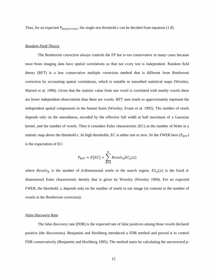
Thus, for an expected , the single test threshold z can be decided from equation (1.8).
Random Field Theory
The Bonferroni correction always controls the FP but is too conservative in many cases because
most brain imaging data have spatial correlations so that not every test is independent. Random field
theory (RFT) is a less conservative multiple correction method that is different from Bonferroni
correction by accounting spatial correlations, which is suitable in smoothed statistical maps (Worsley,
Marrett et al. 1996). Given that the statistic value from one voxel is correlated with nearby voxels there
are fewer independent observations than there are voxels. RFT uses resels to approximately represent the
independent spatial components in the human brain (Worsley, Evans et al. 1992). The number of resels
depends only on the smoothness, encoded by the effective full width at half maximum of a Gaussian
kernel, and the number of voxels. Then it considers Euler characteristic (EC) as the number of blobs in a
statistic map above the threshold z. At high thresholds, EC is either one or zero. So the FWER here ( )
is the expectation of EC:
[ ] ∑
where is the number of d-dimensional resels in the search region, is the fixed d-
dimensional Euler characteristic density that is given by Worsley (Worsley 1994). For an expected
FWER, the threshold, z, depends only on the number of resels in our image (in contrast to the number of
voxels in the Bonferroni correction).
False Discovery Rate
The false discovery rate (FDR) is the expected rate of false positives among those voxels declared
positive (the discoveries). Benjamini and Hochberg introduced a FDR method and proved it to control
FDR conservatively (Benjamini and Hochberg 1995). The method starts by calculating the uncorrected p-

13
value for each voxel and order them that the ordered p-values are . Next, to control the
FDR at α, it finds the largest value k such that
(1.9)
The statistical value corresponding to is chosen as the threshold that all tests greater than or equal to
it can reject their null hypotheses. This procedure requires that at least one null hypothesis is true in the
multiple tests and it is proved to be conservative if the correlations between voxels are positive, which is a
reasonable assumption for most unsmoothed or smoothed imaging data (Yekutieli and Benjamini 1999;
Benjamini and Yekutieli 2001).
GLM in Structure Function Relationships Estimation
Exploring structure function relationships requires explaining one modality of neuroimaging data
using information from other functional or structural imaging modalities. Recently, biological parametric
mapping (BPM) has extended the widely popular SPM approach to enable application of the general
linear model to multiple image modalities (both for regressors and regressands) along with scalar valued
observations (Casanova, Srikanth et al. 2007). In functional and structural neuroimaging, the de facto
standard ―design matrix‖-based general linear regression model and its multi-level cousins have enabled
investigation of the biological basis of the human brain.
BPM uses biological information obtained from one or more imaging modalities, as regressors in
an analysis of another imaging modality in a massively-univariate model. The statistical concepts are the
same as when only response variables are from neuroimage data but using different design matrix in each
voxel (Figure 1.3). The difference in design matrices is due to allowing image data covariates. The
dimensionality of different modality images in a GLM should be the same and the corresponding voxels
should represent the same location in the human brain.

14
GLM in Resting-state fMRI Functional Connectivity
fMRI and SPM are widely used to infer spatial-temporal characteristics of brain activity (Friston,
Jezzard et al. 1994; Friston, Holmes et al. 1995; Worsley and Friston 1995). In addition to task or event
based models, many fMRI studies are now focused on the analysis of resting state activity (van den
Heuvel and Hulshoff Pol 2010).
Since functional communication between brain regions plays a key role in understanding brain
network and structure-function relationships, the analysis of functional connectivity in the human brain is
valued with high importance. The functional connectivity analysis focuses on mapping functional brain
network, examines the relationship among changes in one brain region to changes in others when the
brain is at rest (Figure 1.4). In the resting-state fMRI experiments, volunteers are instructed to relax and
not to think of something in particular, and their fMRI images are acquired. The first study of functional
connectivity using resting-state fMRI is introduced by Biswal (Biswal, Yetkin et al. 1995; Biswal, Van
Kylen et al. 1997), demonstrating functional communication during the left and right hemispheric regions
of the primary motor network. The regions of the brain network are not silent during rest, but show lots of
Figure 1.3 Structure function relationship estimation. The response variable comes from structure or function
images, and at least one explanatory variable comes from other modality images. The value of the design
matrix is different from voxel to voxel.

15
spontaneous activity that their fMRI time course are highly correlated (Cordes, Haughton et al. 2000;
Lowe, Dzemidzic et al. 2000; Greicius, Krasnow et al. 2003).
ReML
In fMRI analysis, the GLM becomes
( ) (1.10)
The error component takes the temporal correlation within one voxel into account and is non-spherical,
because the fMRI time series contain correlated neuronal sources that cannot be modeled or filtered.
Assuming that
∑ (1.11)
The priors can be chose based on any temporal autocorrelation models. A widely used model is the
first order autoregressive model (AR(1)) (Friston, Glaser et al. 2002), which the correlated error having
the time domain form:
(1.12)
where is white noise.The covariance matrix V can be estimated by maximizing the negative free
energy using restrictive maximum likelihood (ReML) method (Friston, Penny et al. 2002). Then it can be
used to pre-multiply the model by a whitening matrix giving:
Figure 1.4 Function connectivity estimation. The explanatory variables that we are interested in are the average
time course signals from a region of interest (ROI). The ROI time course with other confounds are used to
explore the connectivity between the ROI and every other voxels in the human brain.

16
(1.13)
This new model now conforms to sphericity assumptions and can be interpreted in the usual way at each
voxel.
Assumptions in Ordinary Least Squares
OLS is the most widely used method in linear regression analysis, which provides a simple
consistent close form solution of the estimator. To appropriately use the OLS method in the human brain
mapping the assumptions there should be checked beforehand: (1) the errors are independent and
identically distributed normal random variables with zero mean; (2) the explanatory variables are
measured without error or can be considered as without error comparing to the response variable; (3) the
voxels in the brain images are one-to-one correspondence from subject to subject.
Error Assumptions
When there are outliers (e.g., unusual observation), the assumption of normal errors in OLS is
violated. Robust regressions are proposed to deal with this situation that the error components are not
normally distributed. A lot of robust regression methods have been proposed such as M-estimates (Huber
and Ronchetti 1981), Least Median of Squares (LMS) estimates (Rousseeuw 1984), S-estimates
(Rousseeuw and Yohai 1984) and MM-estimates (Yohai 1987). Each robust regression method has their
advantages and disadvantages. Here we only focus on a popular method: M-estimators. M-estimators
assume that the probability density function of the errors is (Press 2007). Then Eq (1.3) becomes:
∏ (
)
(1.14)
where is weight factor, usually denotes standard deviation, is small fixed factor on each data point.
This model can be considered as a general case of OLS. In OLS,
. When outlier comes, r
increases causes that increases rapidly, which influence the estimation of the parameters β a lot. This

17
is why least squares estimates method is sensitive to outliers. In robust regression, does not increase
or increase slowly when r exceeds a threshold, which assigns a small weight to outliers.
In contrast to statistical parametric mapping, non-parametric mapping methods make no
assumptions about the probability distributions of the voxel values being assessed, which may be applied
in situations where less is known about the distribution or the assumption is violated.
Under the null hypothesis, the explanatory variables have no effect on the response variable such
that any orders of the explanatory data will result in the same response. If we assign each explanatory
variable a label, the labels on the data will have exchangeability within the constraints of the randomized
or weak distributional assumptions. The actual labeling used in the experiment (observed statistic) is
randomly chosen from all possible labellings (permutations), so the probability of an outcome is the
proportion of statistic values in the permutation distribution greater or equal to that observed. For
example, if the observed statistic is the largest of the permutation distribution, the p-value is 1/N, where N
is the number of permutations.
For multiple comparisons, the mechanics is computing the maximal statistic of the whole volume
for each possible labeling to create a maximum statistic vector with the length of the number of
permutations. Then the corresponding corrected p-value for each voxel is the proportion of the value in
the maximum statistic vector that is greater than or equal to the voxel statistic.
Regressor Assumptions
When the regressors (explanatory variables) in the GLM are measured with error that cannot be
ignored (e.g., allowing image data in the design matrix), the OLS estimator loses power and the estimated
parameters are not accurate. Instead of minimizing the sum of squares along the response variable in
OLS, Model II regression minimizes a weighted distance along the response and the random explanatory
variables. The principle of Model II regression is first proposed by Deming (Deming 1943) and has been
widely studied in the 2D case. Regression calibration deals with the measurement error problem by
acquiring replicated measurements of the regressors. From these replicated measurements it provides a

18
good estimation of the expectation value of the explanatory variables. Then, the estimated explanatory
value are used in the design matrix instead of measured variables (Carroll, Ruppert et al. 2010).
The problem within the measurement error of the regressors is a bias estimation in OLS so that
can also be solved by SIMulation and EXtrapolation (SIMEX) method. SIMEX is a general measurement
error induced-bias correction method, which is not only suitable for the regression problem. The main
idea of SIMEX is adding additional measurement errors, estimating a trend of bias versus the variance of
the added errors, and then extrapolating this trend back to predict the results when there are no
measurement errors (Carroll, Kuchenhoff et al. 1996).
Voxel-wise Assumptions
The GLM and statistical parametric mapping approach in accessing the neuroimaging inference
assumes a voxel-wise model that requires voxels in each image are all one-to-one correspondence.
Usually, this requirement is met or approximately met through some preprocessing steps. For group
analysis, all subjects are normalized to a template (e.g., MNI-space) and spatially smoothed. For single
subject functional connectivity analysis, all scans are realigned to the first scan or the mean scan through
motion correction.
However, these preprocessing stories still cannot guarantee that the voxels are one-to-one
correspondence unless we have perfect registration algorithms. In the case that a small portion of subjects
are mis-registered, we can treat them as outliers and use robust regression. In the case that we need to
consider spatial correlations in the estimation we can apply a spatial-spectral model (Kang, Ombao et al.
2012).
Our Contributions
The main contributions in the dissertation work are:

19
1. Reliable Statistical Inference in Multi-modality Brain Image Analysis. We addressed the
outlier problems in multi-modality image analysis. Robust statistics have been developed and
accepted in statistics field, but have not been applied in the context of neuroimage study. We
incorporated robust regression into parametric mapping framework to implement a matlab
toolbox with robust estimation and inference methods. We also implemented the non-
parametric permutation tests through the use of cluster computer, to accomplish large
permutation computations on a large volume of voxels. The OLS, M-estimates and the non-
parametric methods are compared in simulation and empirical use. The advantages of the
robust regression are demonstrated as a reliable method that tolerates outliers.
2. Addressing Random Regressors in Multi-Modality Brain Image Analysis. We took
random regressors into account in images on images regression. The statistical theory in
solving the problem is not new; identifying an appropriate model in real word is the science
work we contributed here. We derived a Model II model solution from previous two variable
approach to a general linear model so that the Model II regression can be implemented in the
context of neuroimaging. We demonstrated that Model II regression and regression
calibration approaches are compatible with the design matrix hypothesis testing and multiple
comparison correction frameworks. Besides, we evaluate application of these methods
comparing with OLS in simulation and an empirical illustration in the context of multi-
modality image regression, demonstrating that the random regressors worth consideration in
images on images regression.
3. Robust Statistics and Empirical Validation in Functional Connectivity Analysis. We
proposed a novel approach for quantitatively evaluating statistical inference methods. This
approach can evaluate the performance on empirical data where the truth is unknown and it
does not require acquisition of additional data. In simulation, we proved that this approach is
consistent with type I error and type II error. In empirical applications, this approach showed
that robust regression was not needed in clear empirical 3T rs-fMRI data. However, it acts

20
better than the ordinary least squares estimation on some 7T rs-fMRI data. This approach can
evaluate statistical methods on new problematic empirical dataset without knowing the
specific characteristics of the artifacts (e.g., 7T fMRI) and lead to more reliable statistical
model development.
4. Spatial Temporal Models for Resting State fMRI Analysis. We proposed models that can
account the spatial correlations as well as the temporal correlations in the resting state
functional connectivity analysis within the general linear model framework. The ROI-based
spatio-spectral model for whole brain functional connectivity analysis was extended from a
spatio-spectral model for task fMRI analysis. The voxel-wise spatio-temporal models were
alternative considerations accounting the spatial correlations within a sliding window. The
type I errors were demonstrated to be better controlled using these spatial temporal models
than the one ignoring the spatial correlations. With unsmoothed empirical data studies, none
of the models resulted in expected significance, but our proposed models provided more
accurate estimations and statistical test maps.
5. Multi-Site Brain Image Study. We studied intra-modality and inter-modality brain image
changes in an empirical multi-site large scale data project using mega-analysis and meta-
analysis. We showed that the pre-processed data quality can be assessed through principle
component analysis. After excluding outliers, we can acquire reasonable results from mega-
or meta-analysis. The correlations and difference of the mega- and meta-analysis were
explored. Our robust BPM proved to work well in estimating the relationships between gray
matter density maps and the functional connectivity maps.
Previous Publication
Most contributions of this dissertation have been published. Robust and non-parametric
regressions are discussed in accessing the human brain structure function relationships (Yang, Beason-
Held et al. 2011; Yang, Beason-Held et al. 2011). The applications of the methods are shown (Holmes,

21
Yang et al. 2013). The considerations of the regressor measurement errors in multi-modality neuroimage
mapping are published in (Yang, Lauzon et al. 2011; Yang, Lauzon et al. 2012). Distribution issues in
fMRI are evaluated from empirical datasets (Yang, Holmes et al. 2012). Quantitative evaluations
comparing different inference methods when the truth is unknown are proposed in (Landman, Yang et al.
2012; Yang, Kang et al. 2012; Yang, Kang et al. 2013). The ROI-based spatio-spectral mixed effects
model for resting state fMRI analysis are proposed in (Kang, Yang et al. 2013). The voxel-wise spatio-
temporal models and the multi-site large scale data studies are under preparation.

22
CHAPTER II
BIOLOGICAL PARAMETRIC MAPPING WITH ROBUST AND NON-PARAMETRIC STATISTICS
Introduction
The assessment of structure-function relationships plays an important role in developing
understanding of the human brain. These relationships appear to transcend scales, with connectivity
dynamics appearing at both a micro- (intra-voxel) and macro- (the whole brain) scales (Honey, Thivierge
et al. 2010). While there is firm evidence that structure shapes neural dynamics and function, the
quantitative relationships and how such relationships might be altered in aging and disease remain an area
of active research (Rubinov, Sporns et al. 2009). Statistical parametric mapping and its implementation in
SPM software has emerged as a powerful tool to simultaneously study changes within single voxels and
spatial patterns of activity or tissue volume changes (Worsley, Taylor et al. 2004; Friston, Ashburner et al.
2007). Recently, biological parametric mapping (BPM) (Casanova, Srikanth et al. 2007) and
incorporation of voxel-wise covariates (Oakes, Fox et al. 2007) has enabled multi-modal images to be
analyzed in a manner consistent with traditional voxel-based morphometry. BPM enables regression of
multi-modal images in the same manner that SPM enables regression of images on scalars. In BPM, both
the outcome variables (regressands, ―y‖) and the explanatory variables (e.g., regressors, ―x‖) may be
images, so the design matrices vary voxel-by-voxel. With the BPM approach, one can directly assess the
relationships between images containing functional and structural information. Alternatively, one could
assess the explanatory power of one set of imaging modalities for another.
Violations of the distributional assumptions (such as the presence of outliers) can influence the
results of a statistical analysis considerably, especially when the sample size is small (Friston, Ashburner
et al. 2007). In neuroimaging, outliers can appear both because of imaging artifacts, data processing
anomalies, and non-modeled anatomical differences between brains. In SPM, smoothing is used to

23
compensate for ―uninteresting‖ residual anatomical variability after registration. However, these
anatomical differences are especially problematic in BPM because they introduce systematic and highly
correlated variation in both regressors and regressands. Herein, we implement and evaluate robust and
non-parametric statistical approaches for neuroimaging inference in the presence of outliers and
distributional violations within the BPM regression model.
First, we consider the use of robust statistics for inference. These methods have been well-
established in the statistical literature (Holland and Welsch 1977; Huber and Ronchetti 1981) and are
commonly available in statistical analysis packages (Chen 2002). The general principle of robust statistics
is to use an estimator that is consistent with a traditional, least-squares estimator, but is less sensitive to
distributional assumptions – for example the median is a robust version of the mean. Herein, we extend
the BPM approach to use robust inference with M-estimators (Huber 1964) in place of ordinary least
squares regression. The resulting statistical parametric maps are compatible with the SPM software and
are amenable to standard multiple comparison corrections approaches including random field theory
family-wise error and false discovery rate approaches (Friston, Ashburner et al. 2007).
Second, we investigate non-parametric regression in the context of BPM. Non-parametric
mapping requires minimal assumptions for validity and has been particularly advocated for small-sample
size analysis in the statistical non-parametric mapping (SnPM) implementation (Nichols and Holmes
2002). We apply the SnPM non-parametric regression method within the BPM regression model to
develop biological non-parametric mapping (BnPM). As with robust BPM, the uncorrected statistical
maps are compatible with SPM software and are amenable to standard multiple comparison corrections
approaches if appropriate field theory assumptions are valid. Additionally, the non-parametric approach
offers the ability to perform non-parametric multiple comparison correction based on the maximal
statistic.
This manuscript is organized as follows. First, we introduce the robust and non-parametric
inference theory. Then we describe how these approaches can be used within a voxel-wise framework to
develop robust BPM and BnPM. Simulation examples compare the results from original, robust BPM and

24
BnPM. We close with a discussion of the advantages and limitations of each method and the potential
opportunities for continued innovation.
Methods
BPM enables the use of image on image regression by solving the general linear model (GLM)
with different design matrices for each voxel. This contrasts with conventional SPM (statistical
parametric mapping) which can only use non-image regressors as it uses the same design matrix for a
whole image. By choosing ―regression‖ in the BPM interface, we can evaluate one set of images relative
to another set of images. BPM has been shown to be a promising technique (Casanova, Srikanth et al.
2007) for multi-parametric analysis.
To illustrate the potential short coming, consider two groups of data from one set of subjects
where one subject is mis-registered relative to the remainder of the subjects; Figure 2.1 shows one set of
positron emissions tomography (PET) images and one set of smoothed gray matter (GM) images. If we
examine one voxel within the misregistration region, simultaneous BPM analysis of both datasets suffers
from greatly increased sensitivity to the outlier data as compared to separate SPM of the individual
datasets. In BPM, both regressors and regressands are images which are not fixed, while in SPM, one
regresses scalar values on images, which ensures the regressors are fixed. Both robust regression and
nonparametric regression are promising methods for addressing this outlier problem. To reduce the effects
of outliers, we proposed replacing the ordinary least squares regression method by robust regression, and
using the robust variance to perform robust T-tests and F-tests.
Theory: Robust Regression
M-estimators represent a broad class of techniques which can be considered as the generalizations
of the maximum likelihood framework (Fox 2002). Under the Gaussian distribution and independence
assumptions, ordinary least squares regression is the maximum likelihood estimator. When there are
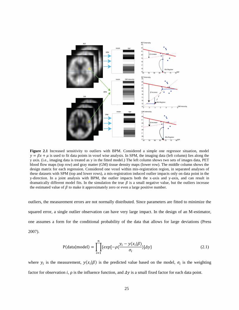
25
outliers, the measurement errors are not normally distributed. Since parameters are fitted to minimize the
squared error, a single outlier observation can have very large impact. In the design of an M-estimator,
one assumes a form for the conditional probability of the data that allows for large deviations (Press
2007).
∏ [
] (2.1)
where is the measurement, is the predicted value based on the model, is the weighting
factor for observation , is the influence function, and is a small fixed factor for each data point.
Figure 2.1 Increased sensitivity to outliers with BPM. Considered a simple one regressor situation, model
𝑦 𝛽𝑥 𝜇 is used to fit data points in voxel wise analysis. In SPM, the imaging data (left column) lies along the
y axis. (i.e., imaging data is treated as y in the fitted model.) The left column shows two sets of images data, PET
blood flow maps (top row) and gray matter (GM) tissue density maps (lower row). The middle column shows the
design matrix for each regression. Considered one voxel within mis-registration region, in separated analyses of
these datasets with SPM (top and lower rows), a mis-registration induced outlier impacts only on data point in the
y-direction. In a joint analysis with BPM, the outlier impacts both the x-axis and y-axis, and can result in
dramatically different model fits. In the simulation the true 𝛽 is a small negative value, but the outliers increase
the estimated value of 𝛽 to make it approximately zero or even a large positive number.

26
The function must be chosen appropriately to achieve the desired effect. If
, the M-
estimator is equal to the least squares estimator. In this case, when an outlier occurs, β is pulled
towards the outlier to minimize ∑
, which makes the least squares estimate method
sensitive to outliers. In robust regression, does not increase or increases slowly when r is greater than
a predefine constant, thus assigning a small weight to outliers which avoids pulling β towards the
outlier. Hence, one seeks a that has lower values in the extreme than a squared term. There are many
weight functions that have been provided and evaluated. The Bisquare weight function and Huber weight
function are both widely used and continuous weight functions. The Huber weight function is monotone,
but assigns a bigger weight to possible outliers. Based on preliminary evaluations of sensitivity to outliers
(not shown), we choose the Bisquare weight function (Beaton and Tukey 1974):
{
(
) * [ (
)
]
+
(2.2)
where C is the tuning constant, usually the value is chosen for 95% asymptotic efficiency when the
distribution of observation error is Gaussian distribution.
Given the robust likelihood model in equation (2.1) and (2.2), we can use the maximum
likelihood algorithm to estimate β. To maximize , we can equivalently minimize
:
∑
(2.3)
Using maximum likelihood method, β should satisfy:
∑
(
)(
) (2.4)
27
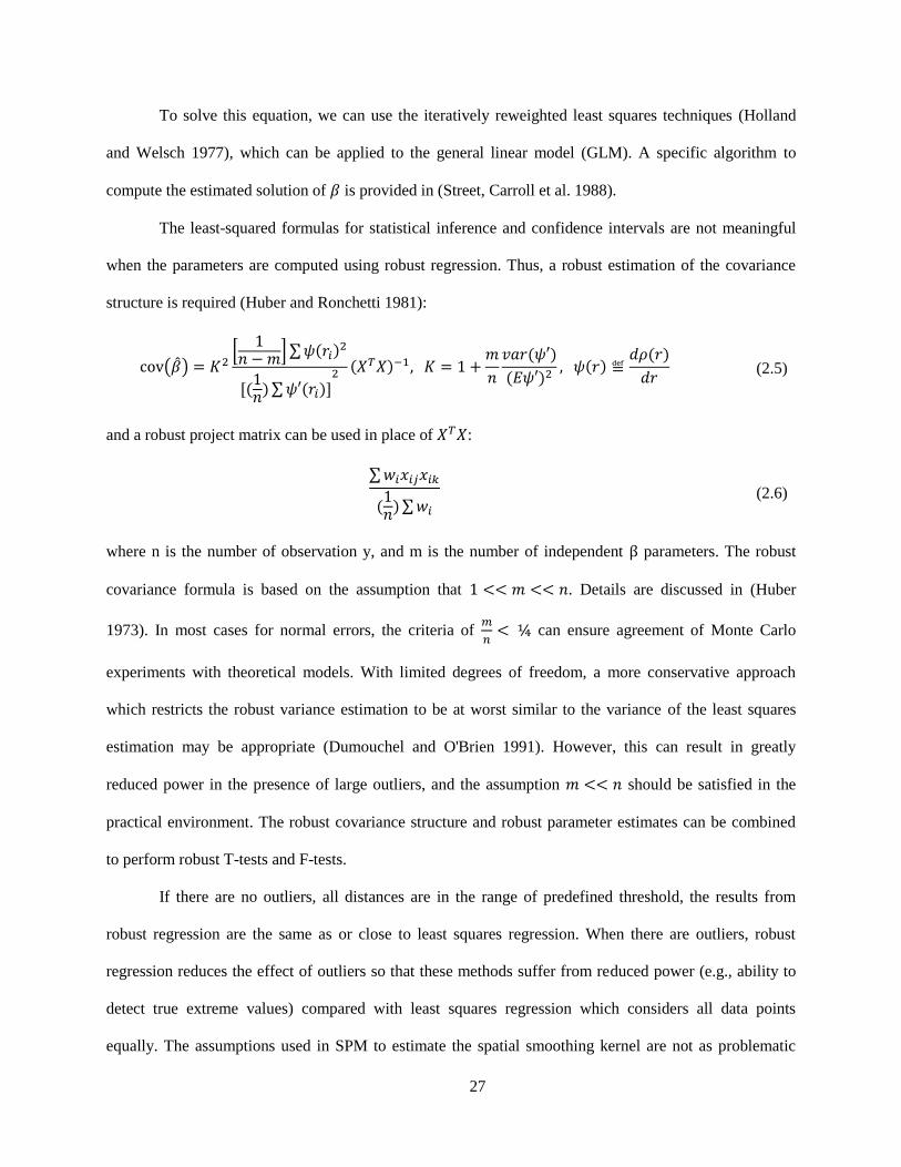
To solve this equation, we can use the iteratively reweighted least squares techniques (Holland
and Welsch 1977), which can be applied to the general linear model (GLM). A specific algorithm to
compute the estimated solution of is provided in (Street, Carroll et al. 1988).
The least-squared formulas for statistical inference and confidence intervals are not meaningful
when the parameters are computed using robust regression. Thus, a robust estimation of the covariance
structure is required (Huber and Ronchetti 1981):
( ) *
+∑
[ ∑ ]
(2.5)
and a robust project matrix can be used in place of :
∑
∑
(2.6)
where n is the number of observation y, and m is the number of independent β parameters. The robust
covariance formula is based on the assumption that . Details are discussed in (Huber
1973). In most cases for normal errors, the criteria of
can ensure agreement of Monte Carlo
experiments with theoretical models. With limited degrees of freedom, a more conservative approach
which restricts the robust variance estimation to be at worst similar to the variance of the least squares
estimation may be appropriate (Dumouchel and O'Brien 1991). However, this can result in greatly
reduced power in the presence of large outliers, and the assumption should be satisfied in the
practical environment. The robust covariance structure and robust parameter estimates can be combined
to perform robust T-tests and F-tests.
If there are no outliers, all distances are in the range of predefined threshold, the results from
robust regression are the same as or close to least squares regression. When there are outliers, robust
regression reduces the effect of outliers so that these methods suffer from reduced power (e.g., ability to
detect true extreme values) compared with least squares regression which considers all data points
equally. The assumptions used in SPM to estimate the spatial smoothing kernel are not as problematic

28
with the outliers as information is pooled across the whole image. However, exploration of robust
smoothness estimation would be a fantastic area of future research.
Theory: Non-parametric Regression
The least-squares approach is based upon the parameterization of the error distribution as
independent and Gaussian. These assumptions are violated by outliers. In contrast, non-parametric
methods make minimal assumptions about the error probability distributions and may be applied in
situations where such assumptions would be inappropriate. Permutation tests have become a widely
popular nonparametric test in neuroimaging through the SnPM software (Nichols and Holmes 2002).
Permutation testing is relevant when data are associated with labels. The hypothesis is that if there is no
effect in the data attributable to the labels, then the probability of the actual label order is equal to that of
any other label permutation. Hence, the statistics associated with each of the possible labelings are also
equally likely. The probability of an outcome as extreme or more than the one observed, the p-value, is
the proportion of statistic values in the permutation distribution greater than or equal to that observed. The
actual labeling used in the experiment is one of the possible labelings, so if the observed statistic is the
largest of the permutation distribution, the p-value is 1/N, where N is the number of possible labelings of
the initial randomization scheme (including the observed one). Herein, we use the same observed statistic
that has been implemented in SnPM5 (Wellcome Department of Cognitive Neurology).
The large number of possible label permutations can be problematic, due to the computations
involved. In situations where it is not feasible to compute the statistic images for all the labelings, a
random subsample of labelings can be used. The set of N possible labelings is reduced to a more
manageable consisting of the true labeling and randomly chosen from the set of N-1 possible
relabeling. Such a test is sometimes known as an approximate permutation test, since the permutation
distribution is approximated by a subsample, leading to approximate p-values and critical thresholds
(Holmes 1994).

29
Random field theory family wise error (FWE) (Worsley, Marrett et al. 1996) and false discovery
rate (FDR) (Benjamini and Hochberg 1995) corrections for multiple comparisons can be inappropriate for
non-parametric methods since there are limited distributional assumptions. Holmes et al. (Holmes, Blair
et al. 1996) provided a single threshold test for permutation multiple comparisons.
Variance estimation for t -statistic can be a noisy process, especially with limited sample sizes.
Since one would expect the noise field to be relatively smooth, one can use a locally pooled variance to
improve accuracy. For parametric methods, use of smoothing would be problematic because it would
require knowledge of the variance-covariance of the voxel level variance structure. Permutation testing
does not suffer from this limitation.
Implementation
The BPM software package was extended to include support for robust regression with Bisquare
M-estimators and non-parametric techniques. In this manner, we extend BPM to form robust BPM
(rBPM) and Biological non-Parametric Mapping (BnPM). BnPM uses non-parametric regression for each
voxel, based on the permutation tests theory. Non-parametric regression calculates p-value based on
randomized permutations (considering the proportion of the numbers with extreme value in permutations)
but not based parametric assumptions. Thus, the direct result of non-parametric regression is a p-value
rather than a T or F statistic. To report BnPM significance results within the SPM software, we invert the
p-value to calculate a T map which can then be mapped back to a p-value in the visualization tools. The
p-value is computed according to the sign of T test (i.e., proportion of the larger numbers for positive t-
test and proportion of the smaller numbers for negative t-test), so the signs of T scores are preserved.
It is important to realize that the computational burden of non-parametric methods is very high.
For a typical image size (e.g., 85*128*64), a modern, single-threaded CPU may require more than thirty
days to compute 10000 permutations. To address this situation, we integrated BnPM with a cluster
processing environment. With BnPM, a regression task (e.g., ―job‖) is divided into many smaller sub-
jobs, each with a specific set of permutation orders for the whole job. Every sub job is considered a new

30
job submitted to the cluster. The number of sub jobs and the execution wall time (i.e., maximum time
allowed for each sub-job completion) is defined by the user and depends on the image size and the
performance of the cluster. The description of each job is written in a format that provides compatibility
to diverse cluster environments and scheduling priorities.
Experiments
First, to demonstrate BPM, rBPM and BnPM in a framework containing outliers, we created 20
simulated images as imaging regressors and another 20 images as the main modality (regressands). The
imaging regressor images were created from one smoothed gray matter image by adding different noise
fields which are generated from Gaussian distribution with zero mean. We define SNR as the mean signal
divided by the standard deviation of noise. We define CNR as the magnitude of the range of voxel
intensities divided by the standard deviation of noise. Figure 2.2 illustrates representative simulated
datasets. The main modality images are created from the regressor images. Inside the head of the caudate
region, the simulated true-intensity of the main modality images is ―1.5*regressor images – constant‖.
Inside the putamen region, the simulated true-intensity of main modality images is ―(-1)*regressor images
+ constant.‖ Everywhere else the simulated true-intensity equals a constant. All constants are chosen to
make SNR = 10 and CNR = 4. To simulate an artifact by mis-registration, one pair of images (e.g.,
Figure 2.2 Simulation design. The normal image (A) shows the regressor images that are created from one
image. The normal image (B) is one of the regressand images. The outlier images (C,D) are rotated around x
(left-right axis) by 15 degrees.

31
representing one simulated subject) are rotated around the x axis (i.e., right-left) by 15 degrees. Then, a
linear model ( ) was fit to evaluate correlations between the pairs of simulated images, and the
null hypothesis of was tested.
Second, to evaluate the relative performance of each method on empirical data, we tested the non-
robust BPM, robust BPM and BnPM (with 10000 permutations) using a sub-set of the normal aging study
of the BLSA neuroimaging project (Resnick, Goldszal et al. 2000). Herein, we used a sub-cohort of 23
healthy participants (14 M/9 F, 60-85 y/o at baseline). Each subject was studied annually for eight years
with T1-weighted MRI sequence (1.5T, GE Medical Systems, SPGR, 0.9375x0.9375x1.5 mm,
256x256x124 mm field of view) and PET data ( , GE 4096+ scanner, 15 slices of 6.5mm thickness,
60s). The baseline scan was denoted as year 1 and the last scan was denoted as year 9. The data were
preprocessed with SPM 5 (http://www.fil.ion.ucl.ac.uk/spm/software/spm5) following steps described in
(Beason-Held, Kraut et al. 2008). The structural scans were normalized to MNI-space, segmented and
smoothed (12 mm Gaussian kernel) to obtain smooth gray matter (GM) density images. PET images were
normalized to SPM's spatial normalization, smoothed (12 mm Gaussian kernel) to MNI-space, and
calibrated for global blood flow measurements to form quantitative cerebral blood flow measurements.
The smoothed gray matter structure images were regressed on the PET data using non-robust BPM,
robust BPM and BnPM to explore the potential for gray matter changes to explain changes in PET
activation levels. Differences between estimated model fits and significance levels of the covariate were
plotted.
Results
As Figure 2.3 illustrates, rBPM and BnPM were incorporated into the BPM software. With the
new user interface, the user has a choice about robust or non-robust regression. If the user chooses robust
regression, we use the iteratively reweighted least squares method to perform M-estimation and compute
robust variances for the GLM model. Otherwise the BPM analysis method remains the same as the

32
original BPM package. If the user selects BnPM analysis, sub-jobs are created using non-parametric
regression method and submitted to the supercomputing cluster. After all sub-jobs are finished, users can
call BnPM results to calculate either uncorrected p-value or corrected p-value.
Table 2.1 summarizes the regression methods studied herein and presents a relative comparison
of analysis time for the empirical example. All toolboxes that have been implemented are listed in the
table with running time compared to the SPM running time. Note that non-parametric methods were set to
use 10000 Monte Carlo permutations rather than exhaustive search. For multi-modality regression, BPM
is the shortest while the BnPM running is the longest. Computation times are listed in terms of a single
threaded CPU. For example, with a grid of 33 computers, the running time for BnPM would be equivalent
to that of rBPM. The robust BPM running time is about 20 minutes for 20 subjects with 79*95*69 size
images. The RobustWLS toolbox for SPM performs robust estimation to compensate artifacts in fMRI
time series data using weighted least squares estimate; this method was not evaluated as this manuscript
Figure 2.3 Software graphical user interface (GUI) and flowchart. With the new software, the user has a choice
between robust regression, non-parametric regression, and traditional least squares regression (shown at left).
Both options make slight modifications to the analysis workflow (right) with the end results of all methods
prepared for visualization within the SPM software package.

33
focuses on data with a single time point (Diedrichsen and Shadmehr 2005).
Table 2.2 shows the sensitivity and specificity of BPM, rBPM and BnPM on simulated dataset
based on uncorrected p-value (p<0.001). The type I error is under control when there are no outliers
(specificity ≈99.9%). When there are outliers, the specificity of BPM is excessively low (lower than
70%) and the sensitivity is also lower. The specificity of rBPM is slightly lower than the theoretical value.
Note that the robust statistics are asymptotically valid, so ability to precisely control type I error improves
with sample size. If rBPM is performed over larger sample size or higher tolerated type I error, the
specificity can be better controlled. BnPM also results is slightly decreased specificity, but has lower
sensitivity than rBPM.
After correcting for multiple comparisons, each of the three regression approaches would lead to
a different conclusion based on inter-modality statistical parametric mapping as illustrated in Figure 2.4.
With traditional BPM, one would see trends towards significant differences in both the region with true
difference (i.e., caudate and putamen) and in the region where outliers were present after multiple
comparisons. The rBPM approach would observe only the true difference. Finally, the BnPM found only
Table 2.1 Comparison of statistical regression methods and available software for neuroimaging Regression Technique
Ordinary Least-Squares Non-parametric:
Permutation Test
Robust: M-estimator
Single Modality
Software Package
SPM (Friston, Ashburner et
al. 2007)
SnPM (Nichols and Holmes
2002)
rSPM (Diedrichsen and
Shadmehr 2005)
Assumptions Modality specific analysis,
data are normally distributed.
Modality specific analysis,
labels have exchangeability fMRI time series data
analysis
Relative computation time
Time 1.0* Time 110 -
Inter- Modality
Software Package
BPM (Casanova, Srikanth
et al. 2007)
BnPM† rBPM†
Assumptions Multi-modality analysis, data
are normally distributed
Multi-modality analysis,
labels have exchangeability
Multi-modality analysis, most
data are normally distributed
but with some outliers
Relative computation time
Time 10 Time: 8 4‡ Time 90
* The total computational time for performing each regression analysis with data corresponding to the
experiment shown in Figure 2.4 (20 subjects, whole brain, 1 mm isotropic resolution, etc.) is reported relative to
the computation time for the traditional SPM approach (approximately 15 seconds on our hardware).
† The highlighted methods represent contributions of this work.
‡ BnPM runs in approximately five hours ―real time‖ on our cluster.

34
a small significant region inside the true difference region after correction for multiple comparisons with
the maximum statistic.
To a large extent, the results found by BPM, rBPM, and BnPM were qualitatively similar using
the empirical dataset as seen in Figure 2.5. However, there were several substantial (and significant)
clusters where the methods reported dissimilar results, two of which are detailed in Figure 2.5.
Conclusions
The presence of outliers and distributional violations in neuroimaging is not a new phenomenon.
Assessing the validity of statistical parametric models in a tractable manner has been paramount in the
design of analysis software (Luo and Nichols 2003). Concerns over the validity of parametric models
have motivated the development of alternative non-parametric approaches (Nichols and Holmes 2002).
These approaches have become widely used for analysis of experiments with small sample sizes. While
Figure 2.4 Simulation results. Results are displayed in SPM in glass brains. The statistical significance is
calculated based on a selected p-value and then projected to three dimensions. Here we display one dimension
of glass brains. The results are shown according to corrected p-value based on random field theory with
p<0.05 and 5 voxels extent threshold to exclude noise. The red region is where there is a positive relationship
and the blue region is where there is a negative relationship. Some points seem to overlap because the map
collapses the out-of-plane dimension.

35
manual data inspection and outlier exclusion are common place, systematic incorporation of these criteria
in the estimation process (e.g., through M-estimators) has not been as thoroughly pursued in
neuroimaging.
In this study, we incorporated robust regression (M-estimation) into BPM to replace ordinary
least-squares regression and implemented BnPM by applying non-parametric permutation tests and using
cluster computation. BPM, robust BPM and BnPM are all integrated in one SPM toolbox so that users can
choose an appropriate regression method for the task at hand. Both simulation and empirical data suggest
increased resilience to outliers in accordance to the theoretical motivationd for these methods.
In the simulation and empirical demonstrations, we demonstrate that these analysis approaches
may lead to differing results. rBPM explicitly tolerates outliers by using robust regression, which makes
the tool reliable against large outliers. However, rBPM still relies on Gaussian assumptions once outliers
are excluded, so the results may not be appropriate for simulations with tenuous distributional
assumptions. Meanwhile BnPM is intrinsically robust to distributional assumptions, but does not
explicitly handle outliers, so it may suffer for lost power in these cases. Note that it would be
straightforward to combine non-parametric and robust regression, i.e., perform permutation testing based
on robust statistics, but this would dramatically increase the computation time.
Table 2.2 Sensitivity and Specificity on simulated dataset
Caudate Putamen
Sensitivity Specificity Sensitivity Specificity
BPM on data
without outliers
99.95% ±0.067% 99.89%±0.11% 97.21%±0.23% 99.87%±0.14%
BPM on data with
outliers
66.38%±0.43% 67.41%±0.84% 81.53%±0.34% 58.03%±1.04%
rBPM on data with
outliers
99.88%±0.12% 99.79%±0.12% 96.63%±0.41% 99.51%±0.20%
BnPM on data with
outliers
72.08%±0.45% 98.77%±0.30% 89.50%±0.36% 98.54%±0.34%
The sensitivity is calculated in the voxels in the true mask and the specificity is calculated in the voxels outside
the true mask but inside the rotated mask. They are computed based on uncorrected p-value (p<0.001). Here we
show the mean value and standard deviation of sensitivity and specificity from 10 simulations (with different
Gaussian noise) for each method.

36
In practical use, the assessment of structure-function relationships will likely involve the presence
of outliers. As significant findings or surprising lack of findings are encountered, it is important to probe
these datasets with robust tools to reveal the potential influence of outliers or distributional violations. For
example, one would want to know if the outliers seen on Figure 2.5 (near 0.8, 20 at left and 0.2, 38 on
Figure 2.5 Empirical Results. Gray matter structural data of 23 participants from year 1 and year 9 (46 images)
were regressed on the PET data of the same subjects. The statistical significance maps are under uncorrected p-
value (p<0.001)and 5 voxels extent threshold to exclude noise. The two plots are the data for one voxel. The
green arrow shows one voxel in the region where non-robust regression indicates non-significance while robust
regression indicates significance. The blue arrow shows one voxel in the region where non-robust regression
indicates significance while robust regression indicates non-significance. The x axis shows the value of GM
structure data and the y axis shows the value of PET data. The red line is the fit of the non-robust regression
while the green line is the fit of the robust regression. The maps in the lower right are the significance maps
with family wise error correction of p<0.05 and 5 voxels cluster threshold.

37
right) are noise, systematic mis-registration, or seemingly valid data points. If these appear valid, is an
important factor missing from the model design? As John Tukey, one of the founders of modern statistics
commented, ―that just which robust/resistant methods you use is not important-what is important is that
you use some. It is perfectly proper to use both classical and robust/resistant methods routinely, and only
worry when they differ enough to matter. But when they differ, you should think hard‖ (Huber 2002).
Here we have provided two very different robust approaches for use in the neuroimaging community. The
described software is available in open source under the Lesser GNU Public License via the NITRC
project ―rbpm‖ (URL: http://www.nitrc.org/projects/rbpm).

38
CHAPTER III
BIOLOGICAL PARAMETRIC MAPPING ACCOUNTING FOR RANDOM REGRESSORS WITH REGRESSION CALIBRATION AND MODEL II REGRESSION
Introduction
The strong relationship between structure and biological function holds true from the
macroscopic scale of multi-cellular organisms to the nano-scale of biomacromolecules. Experience
informs the clinical researcher that such structure-function relationships must also exist in the brain and,
when discovered and quantified, will be powerful informers for early disease detection, prevention, and
our overall understanding of the brain. Brain imaging modalities, such as positron emission tomography
(PET) and magnetic resonance imaging (MRI), are primary methods for investigating brain structure and
function. Quantification of the structure function relationship using imaging data, however, has been
challenging owing to the high-dimensional nature of the data and issues of multiple comparisons.
Statistical Parametric Mapping (SPM) enables exploration of relational hypotheses using the
design matrix paradigm (i.e., ― ‖) without a priori assumptions of regions of interest (ROIs) where
the correlations would occur (Friston, Frith et al. 1990; Friston, Frith et al. 1991). SPM was initially
limited to single modality regression with imaging data represented only in the regressand (i.e., only
varied voxel by voxel) until extensions (e.g., Biological Parametric Mapping, BPM) were developed to
enable multi-modality regression (i.e., to allow to vary voxel by voxel) (Casanova, Srikanth et al. 2007;
Oakes, Fox et al. 2007) and provide for inference robust to artifacts (Yang, Beason-Held et al. 2011).
These multi-modal methods rely on the traditional ordinary least squares (OLS) approach in which
regressors are exactly known (i.e., conditional inference). OLS inference is not inverse consistent;
interchanging the regressor and regressand images would yield different estimates of relationships (as
reviewed by (Altman 1991)). Although conditional inference may be reasonable in SPM, where scalar
regressors are likely to have significantly less variance than the regressand imaging data such an

39
assumption is clearly violated when both regressors and regressand are observations from imaging data
(as in BPM).
Regression analysis accounting for errors in regressors would greatly improve the credibility of
the BPM model by reasonably considering the randomness of the imaging modality in both the regressors
and the regressands. Empirically successful statistical methods accounting for random regressors have
been developed including regression calibration (Carroll, Ruppert et al. 2010) and model II regression
(York 1966; Ludbrook 2010). The specific contributions of this work are that, (1) we implement these
methods (which are established and accepted in statistical community) in the context of neuroimaging, (2)
we demonstrate that these approaches are compatible with the design matrix paradigm, contrast-based
hypothesis testing, and multiple comparison correction frameworks, and (3) we evaluate application of
these methods in simulations and an empirical illustration in the context of multi-modality image
regression. Herein, we focus on multi-modality inference; possible extensions to temporal modeling are
discussed but left as future work.
Notation
For consistency, we have adopted the following notation. Scalar quantities are represented by
italic, lower case symbols (e.g., ). Vectors are represented by bold, italic, lower case symbols (e.g., ).
Matrices are bold, upper case symbols (e.g., ). The symbol is used to note ―distributed as,‖ with
used to represent the multivariate Normal distribution. Subscripts are used to indicate context. For
example, the subscript ―obs‖ indicates the observed value of a random variable. Superscripts are used
with matrices to index columns (i.e., is the vector corresponding to the th column of ) and with
vectors to indicate entries (i.e., is the th element of ). Braces (― ‖) are used to indicate sets,
while ―:‖ is used to indicate vector concatenation and ― ‖ indicates transpose. The hat ( ) indicates an
estimated value of a random variable.

40
Theory
Our aim is to explain the observed intensity from one imaging modality, , with a set of
regressors, , of which at least one member is observed intensity from another imaging modality. We
begin with a typical general linear model (GLM) and reformulate it to explicitly reflect the clinical
imaging case of both random and non-random regressors. To begin, GLM is formulated as,
(3.1)
(3.2)
where is a parameterization of observational error in , is a vector of the fitted coefficients,
ε is the regression error in the model fit, and is the identity matrix. The observation error ( ) and the
equation (or model error) ( ) are assumed to be mutually independent.
Let us consider the columns of the design matrix, , in two disjoint sets: fixed regressors whose
values are considered to be exactly known, , (i.e., the variance in observed values is much less than the
variance of the regressand) and random regressors, , whose observations have non-negligible variance
(i.e., [ ]). Note, must be correspondingly partitioned into and (i.e., [ ]). In
BPM, all regressors in the design matrix are treated as fixed regressors, but in fact, the image intensities
in the design matrix are observed with measurement error. The use of traditional OLS yields a non-
inverse consistent fit, as illustrated in Figure 3.1, due to the model that only considering measurement
errors occur in , but ignoring the errors in . If the roles of and are exchanged, the estimated
coefficients are altered (i.e., the errors are assumed to lie in and the fit is not inverse consistent).
In the more realistic regressor measurement error model, the are not exactly known and
instead are estimated from observations, , containing measurement error:
(3.3)
where is zero-mean Gaussian distributed measurement error with variances . Note
indicates a matrix with diagonal elements corresponding to the given vector. Herein, we will discuss two
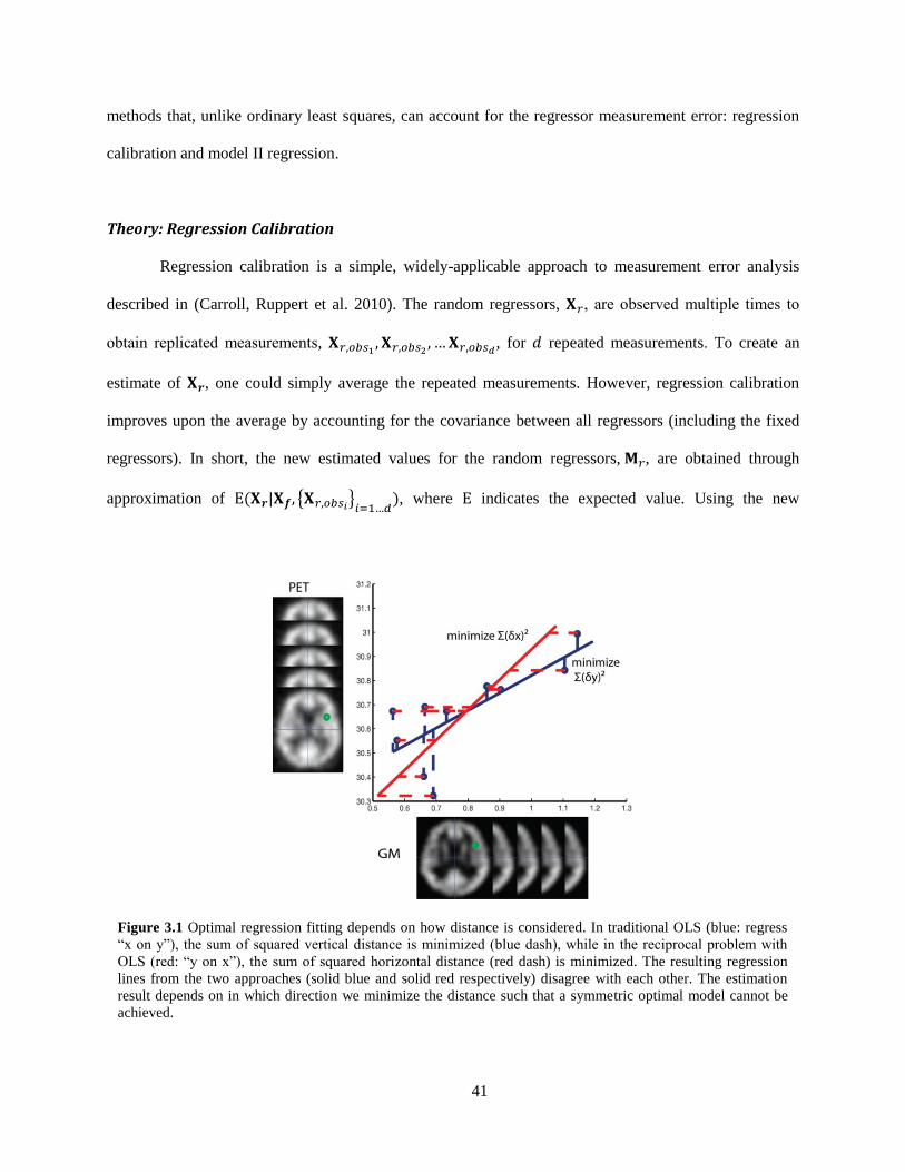
41
methods that, unlike ordinary least squares, can account for the regressor measurement error: regression
calibration and model II regression.
Theory: Regression Calibration
Regression calibration is a simple, widely-applicable approach to measurement error analysis
described in (Carroll, Ruppert et al. 2010). The random regressors, , are observed multiple times to
obtain replicated measurements, , for repeated measurements. To create an
estimate of , one could simply average the repeated measurements. However, regression calibration
improves upon the average by accounting for the covariance between all regressors (including the fixed
regressors). In short, the new estimated values for the random regressors, , are obtained through
approximation of { } , where indicates the expected value. Using the new
Figure 3.1 Optimal regression fitting depends on how distance is considered. In traditional OLS (blue: regress
―x on y‖), the sum of squared vertical distance is minimized (blue dash), while in the reciprocal problem with
OLS (red: ―y on x‖), the sum of squared horizontal distance (red dash) is minimized. The resulting regression
lines from the two approaches (solid blue and solid red respectively) disagree with each other. The estimation
result depends on in which direction we minimize the distance such that a symmetric optimal model cannot be
achieved.

42
approximation of , a standard analysis on the estimated general linear model is performed,
(3.4)
For inference on the significance of estimates, we used the residual bootstrap method as
reviewed in (Carroll, Ruppert et al. 2010).
Theory: Model II Regression
In medical image analysis, especially in functional MRI, it is difficult or impossible to obtain
replicated measurements for . Additionally, replicated measurements are complicated by the increased
resource requirements, increased cost of experimentation, and increased level of volunteer participation.
To work within these constraints and avoid the need for replicated measurements, we consider model II
regression. model II theory diverges from OLS through incorporation of the noise in random regressors
(as in equation (3.3)), and equation (3.2) becomes,
(3.5)
Let be a vector concatenating the observational errors in and in
. Note that the
observational errors, , are errors across subjects and not conditional errors across an image. Given that
each
vector is observed from a unique experimental technique, the elements of are independent
and that the row vectors are also independent across subjects. Therefore, the errors across follow a
multivariate normal distribution (Friston, Holmes et al. 1994):
[
] ∑ (3.6)
Under these assumptions (normal, independent, and identically distributed), the log-likelihood of
the observed data, given the model in equation (3.5) and equation (3.6) is,
( ∑ ) ∑ (
⁄ ( ∑
⁄ ))
∑( ∑
)
(3.7)
where there are subjects (rows of ).

43
Maximizing the log likelihood, equation (3.7), is equivalent to minimizing ∑ ∑
.
With the assumption of independent observations, the covariance matrix, ∑, is diagonal with entries
[
]. Hence, can be re-expressed as,
‖ ‖
∑(
)
‖
‖
(3.8)
where there are regressor random variables and the subscript L2 indicates the L2 norm (i.e., square root
of the sum of squares). Equation (3.8) is minimized when its partial derivatives with respect to each
dependent variable is zero. We first solve for each
by differentiating with respect to
, setting
the result to zero, and using the linear model relation (equation (3.5)). Some manipulation yields,
‖ ( )‖
(3.9)
Equation (3.9) is now independent of the unknown and provides an intuitive form as the error
in the numerator is balanced by the individual variances in the denominator and mirrors the more readily
available multivariate case with non-random X and the univariate case that accounts for one random
regressor (Press 2007). equation (3.9) is a function of two unknown vectors: and σ.
Hence, the variance ratios need to be known in order to minimize s by solving ; otherwise the
system of equations will be undetermined for σ (Carroll and Ruppert 1996). Note that only the relative
variance between observations factors into (as opposed to the absolute variances). If the ratios for
are known (or can be reasonably estimated), then the optimization becomes well defined with an equal
number of unknown to available equations. We employ numeric Nelder–Mead method to optimize with
respect to β. If we add the further assumption that the ratio of the overall measurement error ratio across
subjects is proportional to the ratio of the image noise variance, then we can estimate the measurement
error ratio by estimating the ratio of image noise for each modality. We note that the maximum likelihood
estimate of are asymptotically normally distributed. As reviewed in (Friston, Ashburner et al. 2007), we

44
can use the Fisher information to construct the asymptotic distribution of contrasts of the parameter
estimates (i.e., ) and estimate t-values (and corresponding p-values) for inference.
A common theoretical problem with applications of model II regression is that it is tends to
overestimate the influence of the error of the regressors (i.e., and ) by ignoring the equation error
( ) (Carroll, Ruppert et al. 2010). Here, we partially address this problem by partitioning the total error in
an arbitrary (but reasonably justified) manner according to the relative variances of each measurement
(i.e., versus
). Hemodynamics and/or correlated error models could be addressed in this
framework through estimation and pre-whitening as is typically done with restricted maximum likelihood
approaches for fMRI time series (Friston, Glaser et al. 2002; Friston, Penny et al. 2002), but secondary
noise modeling is beyond the scope of this initial work.
Methods and Results
Regression calibration and model II regression were implemented in MATLAB as an SPM
Toolbox and integrated with a cluster processing environment as illustrated in Figure 3.2. Regression
calibration and model II regression are incorporated as regression method choices in the BPM toolbox for
the SPM software using Matlab (Mathworks, Natick, MA). These modified software and demonstration
data corresponding to the simulation examples are released in open source at
http://www.nitrc.org/projects/rbpm/.
Single Voxel Simulations
Regression Calibration vs OLS
For each of the following single voxel simulation scenarios, a simulated voxel with 50
observations (i.e., subjects) was studied using a model with one random regressor, one fixed regressor,
and a single constant: . In each of 500 Monte Carlo trials, regressors ( and

45
) were chosen randomly from the uniform distribution [0 1], were chosen randomly from the
uniform distribution [0 2], and errors were added to and from a normal distribution with variances
and
respectively. Two measurements for each , ( ) were simulated. OLS was
performed using only the first measurement . Regression calibration was evaluated compared to
OLS with the relative root mean squared error (rRMSE) in ( ), defined over each Monte Carlo
Simulation for regression calibration (RC) and OLS estimates relative to the true (T) parameters:
√∑ ( )
√∑ ( )
(3.10)
A. Regression calibration vs OLS response to ratios (Figure 3.3A). Simulations were
performed varying . Regression calibration performs equally well as OLS with small
, but becomes advantageous as more relative error is introduced into observations.
This advantage is most notable in random regressor coefficient βr.
Figure 3.2 Regression calibration (A) and model II regression (B) address uncertainty in multiple variables.
Regression calibration uses repeated measures to estimate variance in the regressors, while model II regression
relies on an estimation of the relative variance between the regressors and regressands to minimize error.

46
B. Regression calibration vs OLS response to number of random regressors (Figure 3.3B).
The above model was altered by including up to four additional random regressors with
randomized coefficients. Over the model complexity range investigated, regression
calibration has universally smaller errors in all estimated coefficients compared to OLS.
Interestingly, the advantage of regression calibration over OLS for and increased with
increasing model complexity, while the advantage over OLS decreased for .
Regression calibration sensitivity to the number of replicated measurements (Figure 3.3C).
To assess the response of regression calibration to the number of replicated measurements, the number of
random regressor measurements was increased from two to ten. For the increasing number of replicated
measurements, the accuracy of regression calibration for , , and , is improved slightly over OLS.
We note that since the noise on the regressors was Gaussian in this simulation, regression calibration
(which assumes a Gaussian error model) was able to accurately model the variance with limited numbers
of observations.
Model II Regression vs OLS
Model II regression was compared to OLS using a similar model as was used for comparisons
with regression calibration. A simple model with one fixed and one random regressor was used
. For 50 observations, regressors ( and ) were chosen randomly from the uniform
distribution [0 1], βT were chosen randomly from the uniform distribution [0 2] and errors were added to
and from a normal distribution with variances and
, respectively. Model II regression and
OLS are performed on the same dataset. Relative performance of model II to OLS is quantified by the
rRMSE in (equation (3.10)).

47
A. Model II vs OLS response to ratios (Figure 3.4A). Simulations were performed
varying . The performance of model II regression and OLS are comparable for small
, but model II regression becomes more advantageous as more relative error is
introduced into . The improvement is observed specifically on the random regressor
coefficient , whereas the constants not associated with random regressors, and ,
remain with approximately equal accuracy in estimation between the two models.
B. Model II vs OLS response to number of random regressors (Figure 3.4B). The above
model was altered by including up to four additional random regressors with randomized
coefficients (randomly drawn from the uniform distribution [0 2]). Model II has smaller
errors in the βr estimates than OLS; however, model II becomes less advantageous with
increases in the number of random regressors. Note that the number of observations was not
increased to compensate for the increased model complexity; therefore less data per regressor
is available with more regressors.
Figure 3.3 The rRMSE of regression calibration to OLS for each estimated coefficient (𝜷𝒓, 𝜷𝒇, 𝜷𝟏) are plotted as
a function of the ratio of the true standard deviations, 𝝈𝒙 𝒓 𝝈𝒚 (A), the number of random regressors, 𝐗𝒓 𝒋
(B), and
the number of replicated measurements (C). (Note, y-axis was visually optimized for each figure and are not
common across A, B, and C.) With increasing 𝝈𝒙 𝒓 𝝈𝒚 ratios, regression calibration has increased relative
accuracy in 𝜷r estimates compared to OLS. The common simulation shared in (A, B, C) is indicated by a gray
line.

48
C. Model II sensitivity to the estimated ratio (Figure 3.4C). To assess the robustness of
model II against varying levels of accuracy in the ratio estimates, the estimated ratio
of the variance was altered between 1/10th and 10 times its true value, which was set at one.
Under the cases simulated here, model II is insensitive to the ratio mis-estimation range 0.5 to
2, and relatively insensitive over the range 0.1 to 3. At extremely incorrect ratio values, the
estimate rapidly loses accuracy. Based on this analysis we can apply model II regression
using an estimated error ratio, with reasonable confidence in the methods‘ tolerance to mis-
estimation of variance ratios.
Volumetric Imaging Simulation
To explore the performance of these methods on an imaging dataset, we simulated images of two
modalities and regressed one modality on the other modality. The true regressor images are simulated
from smoothed gray matter (GM) density images of 40 participants in the normal aging study of the
Figure 3.4 The rRMSE of model II to OLS for each estimated coefficient (𝜷𝒓, 𝜷𝒇, 𝜷𝟏) are plotted as a function of
the ratio of the true standard deviations, 𝝈𝒙𝒓 𝝈𝒚(A), the number of random regressors, 𝐗𝒓 𝒋
(B) and the accuracy of
the ratio estimate (C). (Note, y-axis were visually optimized for each figure and are not common across A, B, and
C.) With increasing 𝝈𝒙 𝒓 𝝈𝒚 ratios, model II regression has increased relative accuracy in βr estimates compared to
OLS with increasing 𝝈𝒙 𝒓 𝝈𝒚 ratios. In (C), the estimated ratio of𝝈𝒙 𝒓 𝝈𝒚was allowed to deviate from the simulated
value, 𝝈𝒙 𝒓 𝝈𝒚= 1. The common simulation shared in (A, B, C) is indicated by a gray line.

49
Baltimore Longitudinal Study on Aging (BLSA) neuroimaging project consisting of 79x95x69 voxels
with 0.94x0.94x1.5 mm resolution (Resnick, Goldszal et al. 2000). To create repeated measurements for
regression calibration, we simulated two observed regressor images for each subject. OLS and model II
were applied to the first set of measurements. To test the regression methods, a simple model with a
single random regressor and constant was used, . Inside the caudate region:
, inside the putamen: , and for all other brain regions: . The observed regressand
images and the observed regressor images were generated by adding zero mean Gaussian noise across
subjects and the standard deviation used for each voxel was chosen to maintain an SNR around 15 for
each image (SNR is defined as the mean signal divided by the standard deviation of noise).
Figure 3.5 presents the simulated images, the from each method, and the t-map for the
regressor images (the spatial map of the test statistic for the null hypothesis). For clarity, the number of
replicated measurements used for regression calibration was two and the estimated and true ratio for
was one for model II regression. The simulation method was repeated 10 times to create 10
imaging datasets (each of the 10 imaging datasets contained 40 x 2 images and 40 y images). The
Figure 3.5 Simulated imaging associations. The first column shows two noisy regressor images for one subject,
the first measurement is used in OLS regression and model II regression while both of them are used in
regression calibration. The second column shows the paired noisy regressand image. The estimated coefficient β
map and the positive t-map are displayed in the upper right-hand row of and lower left-hand row respectively.
The β and t-maps are shown for OLS, regression calibration (RC) and model II regression. The differences
between the methods are difficult to appreciate in a visual comparison; please see Table 1 for a quantitative
summary.
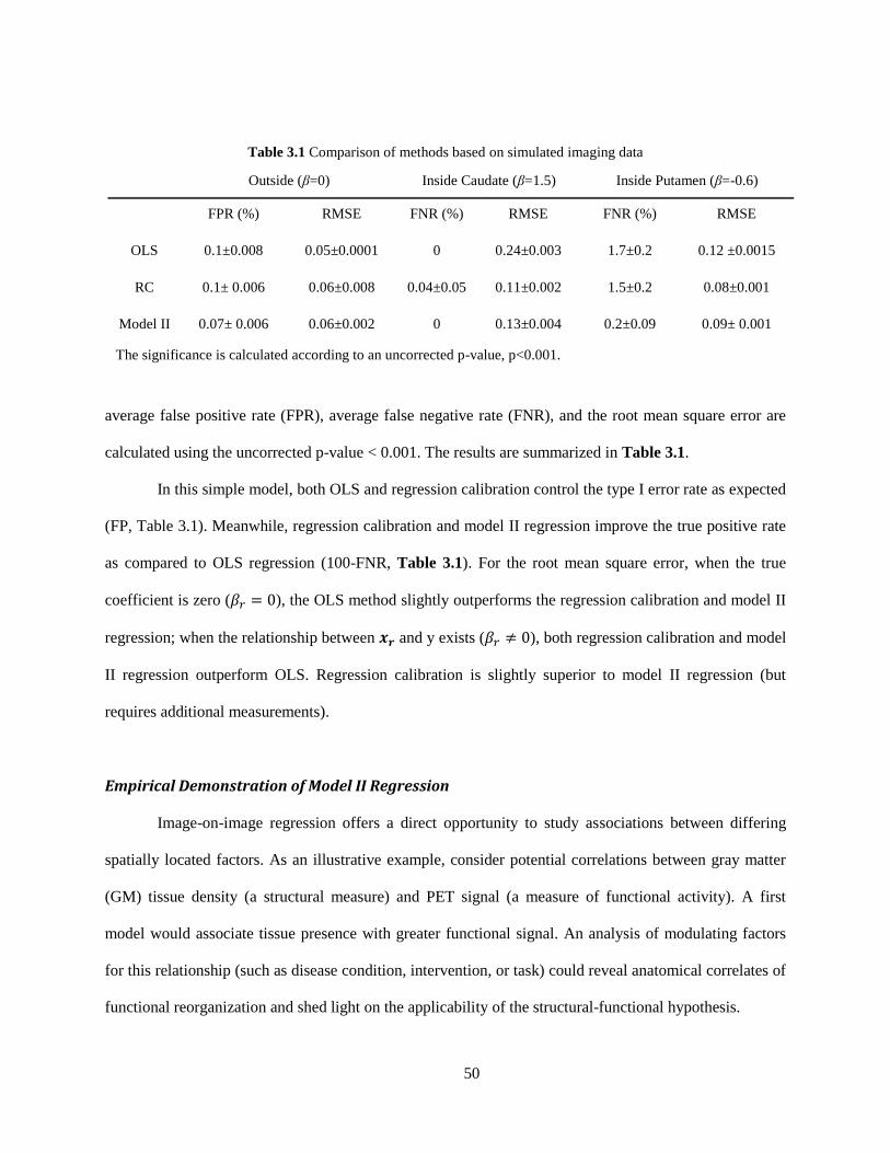
50
average false positive rate (FPR), average false negative rate (FNR), and the root mean square error are
calculated using the uncorrected p-value < 0.001. The results are summarized in Table 3.1.
In this simple model, both OLS and regression calibration control the type I error rate as expected
(FP, Table 3.1). Meanwhile, regression calibration and model II regression improve the true positive rate
as compared to OLS regression (100-FNR, Table 3.1). For the root mean square error, when the true
coefficient is zero ( ), the OLS method slightly outperforms the regression calibration and model II
regression; when the relationship between and y exists ( ), both regression calibration and model
II regression outperform OLS. Regression calibration is slightly superior to model II regression (but
requires additional measurements).
Empirical Demonstration of Model II Regression
Image-on-image regression offers a direct opportunity to study associations between differing
spatially located factors. As an illustrative example, consider potential correlations between gray matter
(GM) tissue density (a structural measure) and PET signal (a measure of functional activity). A first
model would associate tissue presence with greater functional signal. An analysis of modulating factors
for this relationship (such as disease condition, intervention, or task) could reveal anatomical correlates of
functional reorganization and shed light on the applicability of the structural-functional hypothesis.
Table 3.1 Comparison of methods based on simulated imaging data
Outside (β=0) Inside Caudate (β=1.5) Inside Putamen (β=-0.6)
FPR (%) RMSE FNR (%) RMSE FNR (%) RMSE
OLS 0.1±0.008 0.05±0.0001 0 0.24±0.003 1.7±0.2 0.12 ±0.0015
RC 0.1± 0.006 0.06±0.008 0.04±0.05 0.11±0.002 1.5±0.2 0.08±0.001
Model II 0.07± 0.006 0.06±0.002 0 0.13±0.004 0.2±0.09 0.09± 0.001
The significance is calculated according to an uncorrected p-value, p<0.001.

51
Following this approach, we perform regression analysis of the relationship between anatomical
MRI GM images and functional PET images (Beason-Held, Kraut et al. 2008). We used a sub-cohort of
23 healthy participants (14 M/9 F, 60-85 y/o at baseline). Each subject was studied annually for eight
years with a T1-weighted MRI sequence (1.5T, GE Medical Systems, SPGR, 0.9375x0.9375x1.5 mm,
256x256x124 mm field of view) and PET data (GE 4096+ scanner, 15 slices of 6.5mm thickness, 60s).
The baseline scan was denoted as year 1 and the last scan was denoted as year 9. The data were
preprocessed with SPM5 (University College London, UK). The structural scans were normalized to
MNI-space, segmented and smoothed (12 mm Gaussian kernel) to obtain smooth GM density images.
PET images were normalized, smoothed (12 mm Gaussian kernel) to MNI-space, and calibrated for
global blood flow measurements to form cerebral blood for measurements and normalized to [0 1] scalar.
Regression was performed in both directions in order to quantify both structurefunction and
functionstructure relationships. The ―structure‖ data was constructed by concatenating all smoothed
gray matter data for year 1 and year 9 and all subjects, and the ―function‖ data was constructed by
concatenating all corresponding, smoothed, calibrated PET images. Hence, the regression model used one
random regressor and one single constant. Note that this analysis is simplified to illustrate the use of these
methods; a traditional application would also include confounds (age, gender, pre-existing conditions,
year of scan, etc.) and an analysis of time courses and interaction terms. An extended characterization of
the BLSA data is ongoing and beyond the scope of this work demonstrating statistical methods.
As is common in practice, only one measurement for each modality image is available and
regression calibration cannot be applied. The model II ratio is estimated following the method in
(Rajan, Poot et al. 2010), with the window size for the method selected according to the image modality.
The raw data and the resulting OLS and model II regression lines for a single voxel comparison are
displayed in Figure 3.6. The model II regression model is symmetric, i.e., the mapping PETGM is the
inverse of the mapping GM PET while OLS is not. The corresponding estimated variances for model
II are also smaller than the corresponding estimated variances in OLS forward regression and OLS
inverse regression.

52
Conclusions
Properly accounting for error is essential for valid parameter estimation and statistical inference.
Herein, we have demonstrated that a consideration of observation variability is feasible within the
confines of a design matrix paradigm. Furthermore, we can readily consider simultaneous treatment of
parameters with measurement error alongside traditionally defined fixed parameters. Our formulation of
―random observations‖ remains within the context of a ―fixed effects‖ model as the are deterministic
parameters, as opposed to the classic ―random effects‖ model where parameters are stochastic. These two
approaches are complementary and could be combined for an appropriate experimental framework.
Extension of the random regressor concept to time series, hierarchical, and other complex model designs
is a fascinating area for continuing research.
We have observed substantial improvements in model fit using regression calibration and model
II regression as opposed to OLS (Figure 3.3A, Figure 3.4A). While performance of regression
calibration and model II were robust to increasing model complexity (Figure 3.3B, Figure 3.4B) and
prior estimation of observation variability (applicable to model II only, Figure 3.4C), the improvements
were not universal. When the OLS is appropriate (i.e.,
), OLS performs comparable to regression
calibration (Figure 3.3A) and for model II there was a slight increase in observed error relative to OLS
(Figure 3.4A); however, as the relative variance in increased, the OLS assumption of fixed regressors
becomes increasingly violated and increased variance could be observed in the OLS estimates. We
emphasize that the simulations neglect the many of nuances of empirical studies (e.g., correlations among
regressors); these results should be viewed as guide to when alternative regression approaches should be
evaluated as opposed to definitive evidence that a particular method is best suited.

53
On average, differences between the advanced statistical methods and OLS may be subtle as seen
in the parameter estimates and statistical maps in Figures 3.5 and 3.6. As Table 3.1 highlights, OLS
appears quite robust against false positives; however, this may come at the expensive of reduced power
and accuracy. In practice, it is important to consider the impact of the inference approach on individual
voxels, as local findings drive interpretation and consideration of the multiple sources of measurement
error may lead to different parameters estimates and/or different significance values. Model II and
regression calibration can be further adapted to accommodate diverse regression scenarios. For example,
a non-parametric method would be more suitable when the distribution assumptions are unknown
(Nichols and Holmes 2002) while robust regression methods could be applied in the case of outliers
Figure 3.6 Model II and OLS multi-modality regression analysis. OLS (A) and Model II (B) lead to distinct
patterns of significant differences (p<0.001, uncorrected) when applied to identical empirical datasets and
association models. Inspection of single voxel: PET vs grey matter MRI (GM) illustrates the reasons for the
different findings (C). The GLM model used for the forward mapping is 𝒚 𝒙𝒓𝜷𝒓 𝜷𝟏, where 𝒚 represents PET
image intensities and 𝒙𝒓 represents GM normalized image intensities. On the left-hand side of (C), example
images of PET and GM are shown, along with the location of the single example voxel whose regression analysis
is displayed in the right-hand plot. The individual data points (blue circles) were fit using OLS (red lines) and
model II regression (green dashed line). Note that the inverse mapping for OLS (red dash) is not the same as the
forward mapping (red solid line). The model II mapping was found to be reversible and can be represented by the
same line. Resulting error bars and corresponding 𝝈𝒙 𝒓 𝝈𝒚 value estimates are compared between OLS and model
II in the lower right-hand insert.

54
(Huber and Ronchetti 1981; Diedrichsen and Shadmehr 2005; Yang, Beason-Held et al. 2011).
Important areas for further development of model II and regression calibration remain. For
parametric regression, other error models besides Gaussian may be more appropriate for specific imaging
modalities and warrant further consideration. For model II, interpreting the ratio of model variances is a
subject of active consideration as one must consider the potential impact of both the imaging variability
and model fit error in multiple dimensions. As discussed, we currently approximate this combined
quantity as proportional to the imaging variability alone. Developing methods to relax this assumption
would greatly aid in generalization of this approached.
Our presentation of model II regression herein is inverse consistent, provides a logical framework
for exploring relationships in multi-modal image analysis, and can help model relative uncertainty in
imaging methods. Regression calibration accounts for measurement error and has been shown to improve
on OLS in massively-univariate imaging scenarios. The requirement of repeated measurements for
regression calibration makes model II a more likely choice for imaging data where repeat scans are
uncommon. These methods are readily available in open source as plug-ins for the SPM package. Sample
datasets and program documentation are available with the program for download.

55
CHAPTER IV
EVALUATION OF STATISTICAL INFERENCE ON EMPIRICAL RESTING STATE FMRI
Introduction
The exploration of relational changes within the human brain plays an important role in
understanding brain structure and function, helping with disease prediction and prevention. Neuroscience
and patient care have been transformed by quantitative inference of spatial-temporal brain correlations in
normal and patient populations with millimeter resolution and second precision using three-dimensional
structural imaging (magnetic resonance imaging – MRI, computed tomography – CT) and functional
imaging (positron emission tomography – PET, functional MRI – fMRI) (Matthews, Honey et al. 2006).
Classical statistical approaches allow mapping of brain regions associated with planning/execution,
response, and default mode behaviors (through task, event, and resting state paradigms, respectively)
(Friston, Ashburner et al. 2007). When the brain is at rest (i.e., not task driven), functional networks
produce correlated low frequency patterns of activity that can be observed with resting state fMRI (rs-
fMRI). These correlations define one measure of functional connectivity which may be estimated by
voxel-wise regression of activity in a region of interest (ROI) against that of the remainder of the brain
(van den Heuvel and Hulshoff Pol 2010). The selected ROI is called seed. Connectivity analysis has been
widely studied using rs-fMRI and seed method analysis (Bandettini, Jesmanowicz et al. 1993; Biswal,
Yetkin et al. 1995). The sensitivity and specificity of connectivity inference techniques hinge upon valid
models of the noise in the observed data. Yet, in the quest to evermore specifically map neural anatomy,
cognitive function, and potential pathologies, the resolution limitations of the current generation of
clinical MRI scanners are becoming painfully clear – especially in imaging of small structures (e.g.,
(Giove, Garreffa et al. 2004)). The next generation of 7T MRI scanners offers the possibility of greatly
increased signal to noise ratio (SNR) along with higher contrast for functional activity (Hutchison, Leung

56
et al. 2011). Yet, as the magnetic field strength increases, the effects of physiological noise (breath, local
flow and bulk motion), susceptibility artifacts, and hardware induced distortion are increased (Hutton,
Josephs et al. 2011). Hence, artifacts are an increased problem with fMRI at 7T over the current 3T and
1.5T scanners (Triantafyllou, Hoge et al. 2005).
Absolute voxel-wise MRI intensities (arbitrary values) are rarely used in isolation for inference –
rather, the temporal and spatial patterns/correlations of changes over time are of primary interest.
Statistical analyses enable inference of the probability that observed signals are not observed by chance
(i.e., that there exist significant associations between the observed signals and model of brain activity).
The techniques in wide-spread use are based on classical distributional properties (e.g., Gaussian noise
models, auto-regressive temporal correlation, and Gaussian random fields) and have been shown to be
reasonable for well-designed studies at traditional field strengths. Classical statistics here means least-
squares centric approach that lies at the heart of the Statistical Parametric Mapping Matlab toolbox
(Friston, Jezzard et al. 1994; Friston, Holmes et al. 1995). Note that for low SNR, the MRI noise follows
a Rician distribution across an image (Gudbjartsson and Patz 1995; Wink and Roerdink 2006), the Rician
distribution needs to be well considered to provide unbiased estimation when the temporal SNR is low
(Rowe 2005; Zhu, Li et al. 2009). But for the rs-fMRI time series observations the temporal SNR is
usually high enough (>3:1~5:1) so that the approximation of Gaussian distribution assumption is
reasonable (Gudbjartsson and Patz 1995). The discussion of ultra-low temporal SNR is beyond the scope
of this paper. Violations of statistical assumptions threaten to invalidate or (at best) reduce the power of
these experiments. Traditional validation guidance involves careful inspection of residuals and evaluation
of distributional assumptions (Luo and Nichols 2003). When artifacts are detected, images must be
excluded or the analysis approach must be modified. While imaging techniques continue to improve
acquisitions in terms of spatial and temporal characteristics (i.e. resolution, signal characteristics, noise
characteristics), it is uncertain if inevitable tradeoffs resulting in altered noise and artifact levels can be
controlled or compensated for such that their overall impact will be truly negligible.
57
Increased ratio of physiological noise to thermal noise (Kruger and Glover 2001) may increase
the artifacts on 7T fMRI images compared to 3T fMRI. As the prevalence of artifacts increases, the
violations of the Gaussian distribution assumptions over all observations underlying the statistical model
may also increase. In a recent pilot study, we investigated the distributional properties of resting state
fMRI (rs-fMRI) at 3T and 7T (Yang, Holmes et al. 2012). Increasing static field strength from 3T to 7T
provides increased signal and contrast, though this increase is commonly traded for improvements in
spatial and temporal resolution. As such, the resulting data do not necessarily have the same noise
structures, nor are they necessarily well-described by traditional Gaussian noise distribution assumptions.
In fact, the 7T data presented here exhibited substantial non-Gaussian noise structure and spatial
correlations not well-modeled by traditional approaches (as would be expected with data known to be
susceptible to artifacts) (Triantafyllou, Hoge et al. 2005). The statistics literature is ripe with studies
demonstrating ―robust/resistant‖ analysis methods that mimic traditional analyses but are less sensitive to
the impacts of artifacts and errors in distributional assumptions. For example, a robust empirical Bayesian
estimation of longitudinal data is briefly discussed in (Gill 2000) in a non-imaging context and temporal
artifacts have been considered for 3T fMRI by robust estimation of the covariance matrix of the
regression errors (Diedrichsen and Shadmehr 2005). We combined these ideas to extend the traditional
ReML approach to use a robust autoregressive model. Superior performance was demonstrated in
simulation via specificity and sensitivity modeling (e.g., receiver operating characteristic
characterization). When applied to empirical 7T fMRI data, clear differences in statistical parameter maps
were observed between inferences based on classical and robust assumptions. Yet, there is a fundamental
gap between noting empirical differences in statistical parametric maps and concluding that improvement
occurred such that one inference method is more appropriate than another. The problem is illustrated on
an fMRI dataset with a simulated artifact scan in Figure 4.1.
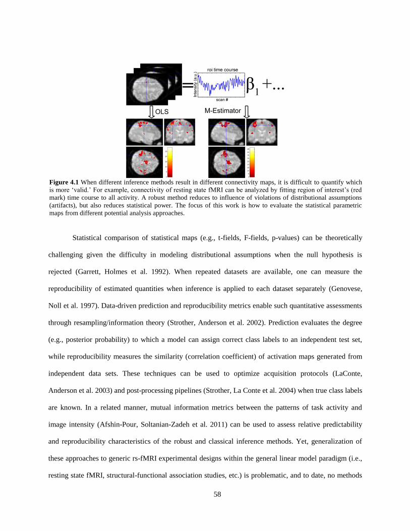
58
Statistical comparison of statistical maps (e.g., t-fields, F-fields, p-values) can be theoretically
challenging given the difficulty in modeling distributional assumptions when the null hypothesis is
rejected (Garrett, Holmes et al. 1992). When repeated datasets are available, one can measure the
reproducibility of estimated quantities when inference is applied to each dataset separately (Genovese,
Noll et al. 1997). Data-driven prediction and reproducibility metrics enable such quantitative assessments
through resampling/information theory (Strother, Anderson et al. 2002). Prediction evaluates the degree
(e.g., posterior probability) to which a model can assign correct class labels to an independent test set,
while reproducibility measures the similarity (correlation coefficient) of activation maps generated from
independent data sets. These techniques can be used to optimize acquisition protocols (LaConte,
Anderson et al. 2003) and post-processing pipelines (Strother, La Conte et al. 2004) when true class labels
are known. In a related manner, mutual information metrics between the patterns of task activity and
image intensity (Afshin-Pour, Soltanian-Zadeh et al. 2011) can be used to assess relative predictability
and reproducibility characteristics of the robust and classical inference methods. Yet, generalization of
these approaches to generic rs-fMRI experimental designs within the general linear model paradigm (i.e.,
resting state fMRI, structural-functional association studies, etc.) is problematic, and to date, no methods
Figure 4.1 When different inference methods result in different connectivity maps, it is difficult to quantify which
is more ‗valid.‘ For example, connectivity of resting state fMRI can be analyzed by fitting region of interest‘s (red
mark) time course to all activity. A robust method reduces to influence of violations of distributional assumptions
(artifacts), but also reduces statistical power. The focus of this work is how to evaluate the statistical parametric
maps from different potential analysis approaches.
59
have been proposed to quantify relative performance of rs-fMRI inference methods based on typically
acquired datasets (i.e., without large numbers of repeated scans for a single subject).
Herein, we characterize empirical, finite sample performance by quantifying the consistency and
resilience of empirical estimators under random data loss (i.e., decimation). These metrics are simple to
compute, readily applied to compare estimators of differing types (robust, non-parametric, classical, etc.),
and provide metrics that enable data-driven estimator selection. These efforts build on recent innovations
in SIMulation and Extrapolation (Carroll, Ruppert et al. 2010) (i.e., SIMEX - the notion that the expected
value of an estimator diverges smoothly with increasing noise levels; therefore, the mean degree of
corruption can be estimated by extrapolating a trend of divergence when synthetic noise is added to
empirical data) and randomized data subsampling. We apply this new technique to characterize ordinary
and robust inference of rs-fMRI data. The proposed approach does not require acquisition of additional
data and is suitable for evaluation on isolated datasets as well as group datasets.
Theory
Terminology
For consistency, we adopt the following notation. Scalar quantities are represented by italic,
lower case symbols (e.g., ). Vectors are represented by bold, italic, lower case symbols (e.g., ).
Matrices are bold, upper case symbols (e.g., ). The symbol ~ is used to note ―distributed as,‖ with N
used to represent the multivariate Normal distribution. The term ―artifacts‖ refers to unusual observations
and the term ―noise‖ is signal not of interest, which may due to physiological or thermal effects. The term
―error‖ refers to the regression error which may or may not contain noise or artifacts.

60
Regression Model
Within this context, we focus on rs-fMRI data, which can be analyzed with an autoregressive
model of order 1 (AR(1)) for a weakly stationary time series (Friston, Penny et al. 2002),
( ) (4.1)
where is a vector of intensity at voxel i, is the design matrix containing seed voxel time
series, is a vector of regression parameters at voxel i, and is a non-spherical error vector. The
correlation matrix is typically estimated using Restricted Maximum Likelihood (ReML) method with a
AR(1) correlation matrix structure, and is estimated on the whitened data (i.e., the ―OLS‖ approach).
Alternatively, a robust estimator (e.g., the ―Huber‖ M-estimator (Huber and Ronchetti 1981)) may be
applied after whitening. Both the OLS and Huber methods are available within the SPM software (Yang,
Beason-Held et al. 2011). Herein, we used the Huber method with the tuning constant chosen for 95%
asymptotic efficiency when the distribution of observation error is Gaussian distribution (Holland and
Welsch 1977).
Monte Carlo Assessment of Inference
Empirical characterization of inference performance when the true value is unknown is a circular
problem – to quantify error, one must have a baseline against which to compare, but, to compute a
baseline from empirical data, one needs an estimator. The SIMEX (Carroll, Ruppert et al. 2010) approach
offers a seemingly implausible, but extraordinarily powerful, shortcut around the issue of unknown
ground truth. The theoretical core of SIMEX is that the expected value of an estimator diverges smoothly
with increasing noise level; therefore, the mean degree of corruption can be estimated by extrapolating a
trend of divergence when synthetic noise is added to empirical data (Cook and Stefanski 1994). Assuming
that the statistical methods under consideration are consistent (i.e., that estimates improve with increasing
information), one can use the marginal sensitivity to information loss (e.g., increasing noise) to compute
the expected estimator bias based on synthetic noise and a single dataset. SIMEX was developed as a

61
general method that is highly adaptable, which has been extended into classification settings (Kuchenhoff,
Mwalili et al. 2006) as well as applied in MRI diffusion tensor imaging (Lauzon, Crainiceanu et al. 2013).
In the context of this study, it is not reasonable to add noise because the noise distributions are uncertain
— especially in the context of artifacts.
If we apply the SIMEX assumption of smooth convergence to the problem of imaging inference
with unknown noise / artifact distributions, we can probe the marginal reduction in sensitivity of an
estimator by removing data. We define resilience as the ability of an inference method to maintain a
consistent parametric map estimate despite a reduction in data. Over the time course of an rs-fMRI
experiment (5-10 mins), the active brain regions vary. Hence, reproducibility of inferences based on
sampled time periods (e.g., first versus second half) are not meaningful. Therefore, we focus on
diminishing random data samples as opposed to structured temporal resampling. The number of
diminished scans is small and Monte Carlo simulations procedures are used to estimate the mean
Figure 4.2 Representative one voxel t-values as data is randomly decimated. An rs-fMRI dataset is randomly
diminished into N data size levels with M subsets in each level. Inference methods are applied to each subset to
estimate voxel-wise t-maps. The highlighted point (left) indicates the rs-fMRI seed region.

62
marginal impact using many different randomly decimated data. Examples of subsampling for one voxel
t-value are displayed in Figure 4.2.
The scans are randomly deleted after all pre-processing steps so that the changes of scan intervals
do not affect the slice timing correction or low pass filtering. Recall that the temporal covariance of fMRI
time series is estimated using ReML with a AR(1) correlation structure. To address the scan interval
changes we modified the temporal correlation matrix according to the number of time points between
every two image. In SPM, low frequency confounds are removed before estimation using residual
formatting matrix. To address random data removal, we generated the low frequency filtering matrix for
the whole data then deleted the time points corresponding to the scans removed.
Resilience
An intuitive way to assess the resilience of an inference method to a reduction in data might be to
calculate the absolute value of the difference between the mean t-values (across Monte Carlo simulations)
as a function of data size. However, this method will result in higher difference when the t-value with all
data is high versus the t-value with all data is low as data reduction will universally pull t-values away
from significance. Such an approach will strongly depend on the true effect size and the mean t-value
cannot reflect the resilience to the artifacts if any (Yang, Kang et al. 2012). Hence, it is important to also
consider the variance of the estimated parametric maps – we advocate evaluating the resilience in terms of
consistency and variance.
Small reductions in data result in approximately linear reductions in t-value (due to smooth loss
of power – not shown), so we advocate focusing on a specified diminished data size (e.g., randomly
diminished by 10% and 20%) rather than on a large number of different data decimations. At a single data
size with 10% decimation we have three parametric maps of data across all spatial locations; one t-map of
the starting t-values, one t-map of the mean t-value from the Monte Carlo repetitions, and one variance
map from the Monte Carlo repetitions. The right subplots in Figure 4.2 show one slice of the t-map fields
with the mean and the variance of the t-value over the subsamples.

63
Consistency assesses the bias of the computed parametric map of the decimated data relative to
the same map computed with complete data. A priori, one would expect to see small reductions in
parametric map values between the complete and decimated datasets due to power loss, but there would
be few large changes as both classical and robust inference methods are reasonably unbiased. We
summarize consistency by pooling information across all in-brain voxels using linear regression:
(4.2)
where is a vector containing one t-value for each in-brain voxel where the t-value is estimated
using the overall time series, is the mean t-value of all subsamples (across Monte Carlo iteration) and
the slope reflects the pooled consistency (Figure 4.3). If the inference method is consistent,
should be close to one and the fitting error would be small. The value of can therefore be viewed as a
reflection of bias with the sign indicating positive or negative bias and the R-squared can assess the
Figure 4.3 Illustration of consistency estimation. The mean t-value of random subsamples with 10% diminished data
(vertical) is plotted versus the t-value with all data (horizontal). The left plot displays the OLS estimates and the
right shows the M-estimates. The dashed line indicates equality (𝑦 𝑥); the data points above the dashed line have
positive bias and the points below the dashed line have negative bias. The solid line is the estimated regression line
from all the data points in each plot.

64
goodness of fit relative to the random error ( ). As we are losing data, we can expect lower t-values for
significant voxels, thus will not equal one but should be close to one. Hence, a statistical test is not
appropriate – we know the true distributions are different – rather, we must use the numerical value of
in a qualitative assessment.
The variance of the Monte Carlo t-values can reflect how resistant an estimation method is to
artifacts in the dataset. If a method is affected by artifacts, the variance will increase when artifacts exist.
This is because the artifacts may appear in some subsamples while not in others which will result in
varied t-value estimates. Although the inference method with overall smaller variances is more resistant
to artifacts, the artifacts may exist only in some brain regions. These regional effects are difficult to detect
from looking directly at a variance map as in Figure 4.2. To account for the influence of regional or a
small number of artifacts, the variances from two inference methods are compared directly (Figure 4.4).
The collection of variance values across spatial locations for inference method-1, , (e.g., OLS) is
plotted against those of inference method-2, , (e.g., robust) and their variances are compared by
Figure 4.4 t-value variance comparison. The variance of subsample t-values with 10% diminished data from OLS
(horizontal) and robust estimation (vertical) methods are compared. The dashed line (𝑦 𝑥) shows when the
variance from the OLS and robust method are equal. The solid line is the estimated regression line.

65
computing the slope between them under consideration of random error ( ).
(4.3)
If these two methods are equivalent, the slope will be close to one. If the slope is larger than one,
the method-1 is superior; on the contrary, if the slope is smaller than one, the method-2 is superior. The
slope is impacted when one method contains spatial locations with larger variance which may due to the
impact of artifacts. Figure 4.4 displays two examples, and Figure 4.5 presents corresponding brain
images indicating the spatial locations where the variance from robust estimation is lower than the
variance from OLS.
When using robust regression, we have to pay the price that it is 95% asymptotically Gaussian
when there are no artifacts (i.e., 5% reduction in power). To compare the OLS and robust variance, we
selected the variance from OLS as and the variance from Huber estimation as in
(equation (4.3)), if the slope is less than one, the robust estimation is practically superior to OLS
estimation.
Methods and Results
Simulation Experiments
Simulation Data
To investigate the properties of our method in a controlled environment, we first performed
simulation experiments. In the simulation a simple regression model is used:
(4.4)
where simulates the seed voxel time course, is the connectivity coefficient, and is the
normalized covariance matrix. is simulated from an empirical 3T unsmoothed fMRI data. (The
source fMRI data are preprocessed through slice timing correction, realignment and normalized to MNI

66
space.) We selected a voxel inside the right motor cortex and acquired its time series. The time series was
demeaned to simulate the value of . The mean value of the original (un-demeaned) voxel time course
is about 905 (arbitrary intensity units), and the standard deviation is about 11. So we designed the
simulated temporal signal to noise ratio (TSNR) to be 80:1 (≈ 905/11). We used 8 for other voxels
( for the seed voxel) inside the right side of gray matter (GM), for the voxels inside the
left side of GM, and for the rest of the brain. The mean value of a white matter voxel time course
is about 800 so is set to make the whole brain mean value to be around 800. We calculated based
on these parameters.
(4.5)
For each voxel, we generated Gaussian noise for the first time point, and then
convolved the Gaussian noise to generate autoregressive noise with correlation 0.2 across time. is
chosen to make TSNR ≃ 80:1. We added the autoregressive noise to the to simulate fMRI images.
In this simulation, the AR(1) parameter is constant for all voxels, but the estimation method does not
estimate the AR(1) parameter, instead, it estimates the covariance matrix of the temporal noise (Worsley,
Liao et al. 2002). The seed voxel time course is considered as the design matrix.
To simulate artifacts, we created an outlier scan by adding Gaussian noise with higher standard
Figure 4.5 t-value variance comparison corresponding brain images. The red points represent where variance from
robust estimation that is lower than the variance from OLS. (A) corresponds to Figure 4.4A and (B) corresponds to
Figure 4.4B.

67
deviation to a simulated scan. The outlier scan is chosen with the highest seed intensity and the noise is
only added to a region of the brain. The added Gaussian noise is zero mean with standard deviation 10
times the standard deviation of the original simulated scan. Other simulated scans are kept the same.
Subsample Parameters and Simulation Result
User controlled parameters for implementing our method include (i) the number of Monte Carlo
simulations and (ii) the diminished data size. To decide the number of Monte Carlo simulation and the
diminished data size, we evaluate their influence on the consistency and the variance on simulation data
as shown in Figure 4.6. To decide the number of Monte Carlo simulations, we plotted the for the
OLS consistency (equation (4.2)) and for the variance comparison (equation (4.3)). Plots were
made for two variance comparison across five similar simulations when 10% of scans are randomly
diminished. When there is only one Monte Carlo simulation, the range of the boxplot is large and it
decreases as the number of Monte Carlo simulations increase.
The consistency from the OLS and the robust (not shown in the figure) inference are similar with
and without outliers if the number of Monte Carlo simulations is over 50. When there are no outliers, the
variance slope is greater than one, which suggests the OLS method is better than the robust method.
When there are outliers, the is less than one, which suggests the robust method is better than the
OLS method.
Empirical Experiments
Empirical Data
For illustrative purposes, we consider 15 distinct in vivo datasets.
Seven representative healthy subject rs-fMRI acquired at 3T were downloaded from
http://www.nitrc.org/projects/nyu_trt/ (197 volumes, FOV = 192 mm, flip θ = 90°, TR/TE = 2000/25 ms,

68
3x3x3 mm, 64x64x39 voxels) (Shehzad, Kelly et al. 2009). Prior to analysis, all images were corrected
for slice timing artifacts and motion artifacts using SPM8 (University College London, UK). All time
courses were low pass filtered at 0.1 Hz using a Chebychev Type II filter, spatially normalized to MNI
space, spatially smoothed with an 8 mm FWHM Gaussian kernel, linearly detrended, and de-meaned. The
3T data are smoothed, a typical pre-processing step for 3T fMRI to increase spatial SNR. Two voxels
inside the right primary motor cortex for each subject were manually selected as the region of interest
(ROI) by experienced researchers through exploring the unsmoothed images and comparing with the
standard atlas. The design matrix for the general linear model was defined as the ROI time courses, the
six estimated motion parameters, and one intercept. To create whole-brain connectivity maps, every
labeled brain voxel underwent linear regression using the design matrix.
Eight normal subjects were studied at 7T after informed consent. Subjects were instructed to both
close their eyes and rest. Briefly, the resting state images were acquired for 500s using single shot
Figure 4.6 Influence of resilience parameter. (A) shows the impact of the number of Monte Carlo repetitions with 10%
diminished data. (B) shows the impact of the diminished data size level when we performed 50 Monte Carlos each time.
The OLS consistency plots display the slope 𝛽𝑚𝑒𝑎𝑛 in equation (4.2). The variance comparison plots display
𝛽𝑣𝑎𝑟 , where 𝛽𝑣𝑎𝑟 is the slope of variance from robust estimation on OLS. ―With\without artifacts‖ indicates if there
are simulated outlier scans in the simulation.

69
gradient echo EPI (500 volumes, FOV = 192mm, flip θ = 53.8°, TR/TE = 1000/28ms, SENSE factor =
3.92, full k-space acquisition, resolution 2x2x2mm, 96x96x13 voxels). Prior to analysis, all images were
corrected for slice timing artifacts and motion artifacts using SPM8 (University College London, UK).
All voxels‘ time courses were low pass filtered at 0.1Hz using a Chebychev Type II filter, linearly
detrended, and de-meaned. The 7T data are not smoothed because the spatial SNR are much higher in 7T
than 3T, and we are only interested in single subject results that smoothness is not necessary. The seed
voxel was defined as a single manually selected voxel located in primary motor cortex along the central
sulcus that was also significantly activated by a conventional finger tapping task contrasting bimanual,
self-paced finger tapping against a resting condition (FWE corrected, p < 0.05, minimum cluster size = 1
voxel) (Newton, Rogers et al. 2012). The design matrix for the general linear model was defined as the
seed voxel time course, the six estimated motion parameters and the intercept. Each voxel‘s BOLD time
course underwent linear regression of the design matrix to create connectivity maps.
Comparative Analysis of Classical and Robust Inference
rs-fMRI analysis was performed on each dataset in SPM8 using ordinary ―OLS‖ and robust
(―Huber‖) regression methods. For each decimation level (10% and 20%), 50 Monte Carlo simulations
were performed. For each Monte Carlo simulation, a subset of either 90% or 80% of the total data was
randomly selected, the OLS and Huber estimation methods were applied, and the t-maps on the
coefficient for the ROI time courses were stored. Consistency was assessed between the mean of the
decimated maps and the map using all data, while the relative variance was assessed between Monte
Carlo simulations with each method. For the resilience variance metrics, OLS was on the x-axis and
Huber on the y-axis. Note that both OLS and Huber were fit to the same subsample of the data (i.e., the
random subsamples are paired).

70
Empirical Results
Representative statistical parametric maps from OLS and robust regression of one 3T fMRI and
two 7T fMRI are displayed in Figure 4.7. Noted that the results are shown on uncorrected p-value
without cluster size threshold, the difference between results from OLS and robust regression may be
more obvious than the results after cluster threshold. The results of all subjects are shown in Table 4.1.
Next, we discuss how the qualitative metrics may be used for selection of inference method.
• For subjects 1 to 7, 10, 13, the consistency estimates are similar and close to zero for both
OLS and Huber, while the R2 value is high. This indicates that neither method is particularly biased by
the decimation process. The variance matrices for both 10% and 20% decimation are negative except 20%
decimation for subject 3, which indicates that OLS was more resilient than Huber. The variance metric for
20% decimation for subject 3 is positive, but the value is too small (<0.01) to show any interest.
Conclusion: Robust inference is not necessary; OLS is preferable. When there are no
outliers, the OLS method is better than the robust method because the robust method is only
approximately 95% as statistically efficient as the OLS method. The evaluation conclusion indicates that
there are relatively few outliers in this data set.
• For subjects 8, 15, the consistency estimates are similar and close to zero for both OLS
and Huber, and the R2 value is high. Hence, neither method is particularly biased by the decimation
process. The variance metric for both 10% and 20% decimation is positive, which indicates that Huber
was more resilient than OLS.
Conclusion: Robust inference yields higher resilience and should be used. It indicates that
there are outliers in this data set. Since the probability of the existence of outliers increase at 7T compared
to 3T it is not surprising that the robust inference method is better than the OLS.
• For subjects 9, 11, 12, 14, the consistency estimates are similar and close to zero for both
OLS and Huber, and the R2 value is high. Hence, neither method is particularly biased by the decimation
process. The biases at 20% decimation are always higher and the R2 value is lower than at 10%
decimation for all these subjects. For subject 9, 12, 14, the variance metric for the 10% decimation is
71
marginally positive while the variance metric for the 20% decimation is negative. For subject 11, the
Table 4.1 Summary of Resilience Measures for All Subjects
subject diminished data Method Consistency Variance
𝛽𝑚𝑒𝑎𝑛 𝑅 𝛽𝑣𝑎𝑟
1
(3T)
10% OLS -0.016 0.992
-0.113 Huber -0.018 0.991
20% OLS -0.050 0.984
-0.179 Huber -0.049 0.981
2
(3T)
10% OLS -0.078 0.975
-0.067 Huber -0.071 0.980
20% OLS -0.138 0.950
-0.244 Huber -0.133 0.951
3
(3T)
10% OLS -0.019 0.989
-0.083 Huber -0.022 0.990
20% OLS -0.051 0.961
0.006 Huber -0.053 0.965
4
(3T)
10% OLS -0.108 0.965
-0.034 Huber -0.110 0.962
20% OLS -0.189 0.888
-0.067 Huber -0.195 0.882
5
(3T)
10% OLS -0.040 0.983
-0.123 Huber -0.044 0.973
20% OLS -0.095 0.946
-0.013 Huber -0.101 0.939
6
(3T)
10% OLS -0.074 0.968
-0.165 Huber -0.076 0.970
20% OLS -0.161 0.898
-0.148 Huber -0.169 0.891
7
(3T)
10% OLS -0.074 0.964
-0.052 Huber -0.076 0.963
20% OLS -0.140 0.911
-0.056 Huber -0.142 0.904
8
(7T)
10% OLS -0.054 0.999
0.579 Huber -0.057 0.999
20% OLS -0.119 0.997
0.280 Huber -0.120 0.995
9
(7T)
10% OLS -0.051 0.995
0.029 Huber -0.049 0.995
20% OLS -0.115 0.964
-0.106 Huber -0.107 0.968
10 (7T)
10% OLS -0.091 0.996
-0.373 Huber -0.107 0.981
20% OLS -0.175 0.986
-0.389 Huber -0.177 0.963
11
(7T)
10% OLS -0.066 0.999
-0.328 Huber -0.056 0.998
20% OLS -0.126 0.995
0.177 Huber -0.106 0.995
12
(7T)
10% OLS -0.125 0.980
0.550 Huber -0.089 0.987
20% OLS -0.176 0.962
-0.158 Huber -0.156 0.964
13
(7T)
10% OLS -0.037 0.997
-0.250 Huber -0.031 0.997
20% OLS -0.050 0.990
-0.088 Huber -0.033 0.989
14
(7T)
10% OLS -0.170 0.980
0.285 Huber 0.050 0.968
20% OLS -0.223 0.962
-0.054 Huber 0.038 0.932
15
(7T)
10% OLS -0.059 0.996
0.220 Huber 0.012 0.977
20% OLS -0.113 0.990
0.169 Huber -0.046 0.959
72
variance metric for the 10% decimation is negative while the variance metric for the 20% decimation is
positive. The mixed results indicate that neither method is clearly superior and that careful data inspection
is warranted.
Conclusion: Robust inference may be desirable, but OLS could be suitable. The similar
performance of the robust and the OLS methods may due to the fact that there are outliers but the number
is small. In that situation, the OLS is better in most brain regions but the robust inference is much better
in some small regions. Both methods yield acceptable results.
Discussion and Conclusions
The proposed resilience metrics provide a quantitative basis on which to compare inference
methods. The simulation results suggest that a comparison of methods based on resilience would yield
similar conclusions as one based on the sensitivity and specificity matrix. Yet, resilience is accessible for
empirical data, when the ground truth (necessary for sensitivity and specificity) is rarely known. It is
reassuring to see that resilience also indicates that OLS would outperform the robust inference approach
on the 3T dataset where few outliers exist. For the 7T dataset the robust approach would outperform OLS
since the achievable signal to noise ratio increases and the propensity for artifacts increases.
In simulations, it is easy to construct realistic datasets demonstrating that classical assumptions
are sufficient or insufficient. However, in reality, it is very difficult to assess the stability of the
robust/non-robust decision to variations in artifacts. Hence, creating representative artifact-prone
distributions is a substantial endeavor. It is possible to acquire a massive reproducibility dataset and use
this dataset to produce a highly robust ground truth estimate. Given such data, one may map artifact
distributions. However, such acquisitions are exceedingly resource intensive and may not be
representative of other sites and/or acquisitions. Hence, generalization of artifact findings is problematic.

73
However, the proposed resilience consistency and variance metrics provide a quantitative basis
on which to judge individual datasets, allowing one to evaluate suitability of particular inference
mechanisms on initial pilot data. This could be done in case studies, or as part of multi-level analysis to
evaluate the tradeoffs between improved power (when classical assumptions are met) and reduced
susceptibility to artifacts, based on actual empirical data.
Consistency in statistics is defined as convergence in probability, i.e., a consistent estimator of
parameter converges to its true value as sample size grows. However, in practice it is not feasible to prove
the consistency of an estimator because the truth remains unknown. What we assessed in this paper is not
the absolute consistency but rather the relative consistency as it related to resilience of estimator, which
could be achieved when estimated values were relatively stable regardless of the amount of data used as
Figure 4.7 Representative overlays of significant for three subjects (columns) with OLS (top row) and robust (lower
row) estimation methods. The connectivity maps are computed from one-sided t-test on the ROI time course
coefficients (𝑝 , uncorrected). The blue circle shows the OLS result is significant while the robust result is
not or less significant. The green circle shows the robust result is significant while the OLS result is not or less
significant. Resilience measures are tabulated in Table 4.1.

74
illustrated in Section II. We are not intending to empirically prove that the robust estimator is a
absolutely consistent, but we want to show that estimates based on the robust estimator can be more (or
less) consistent (or invariable) than another as decimated data are utilized.
Generally, the evaluation result depends on the number of effective outliers in the brain. In some
cases, the evaluation is location dependent such that one estimator is good for one seed but not good for
another, especially when outliers exist in one region but not in others. The resilience method still can be
used to evaluate inference methods (e.g., see Figure 4.5), albeit without the increased power gained by
pooling regions.
The random decimation procedure can be problematic for aspects of temporal estimation. We
initially sought to examine split half (either temporal: early/late or frequency: even/odd). Unfortunately,
both lead to systematic differences in the quantities being estimated by rs-fMRI. Temporal subsampling
dramatically reduces the sensitivity to low-frequency correlations (which are of primary interest) and
focuses analysis on short time periods with potentially different biological states. Frequency subsampling
reduces the intrinsic sensitivity to temporal frequencies and imparts differing sensitivity to artifact. We
examined a number of different random decimation methods and propose random decimation as a
compromise between empirical power (i.e., we see differences where ones are known to exist) and ease of
use.
Implementation of this approach requires the ability to decimate (remove) data randomly, loop
over multiple possible data subsets, and calculate summary measures of the resulting statistical fields.
With modern multi-core and cluster environments, a 50-100 fold increase in the computational burden of
a traditional analysis is not typically problematic for off-line analysis. For example, the experiments
presents one OLS analysis takes approximately 40 seconds and one Huber analysis takes 100 minutes.
With proper parallelization, the total wait time would not be substantively longer than the time for a
single analysis.
In conclusion, we have presented a novel approach for quantifying inference methods based on
empirical data. We evaluated the resilience of the ordinary (OLS) and a robust method (23) for both

75
simulated and empirical data. Resilience provides a simple, but powerful method for comparing a proxy
for accuracy of inference approaches in empirical data where the underlying true value is unknown.
Statistical theories characterizing finite sample statistical behavior are undergoing rapid and exciting
developments in the statistical community. These statistical methods, encompassing SIMEX, bootstrap,
and Monte Carlo approaches, offer the potential to understand both the uncertainty and bias in metrics
estimated from imaging data. Given the abundance of computational power generally available, these
methods can now be feasibly applied on routine basis.

76
CHAPTER V
WHOLE BRAIN FMRI CONNECTIVITY INFERENCE ACCOUNTING TEMPORAL AND SPATIAL CORRELATIONS
Introduction
Neuroscience and patient care have been transformed by quantitative inference of spatial-
temporal brain correlations in normal and patient populations with millimeter resolution and second
precision using functional MRI (fMRI) (Matthews, Honey et al. 2006). Classical statistical approaches
allow mapping of brain regions associated with planning/execution, response, and default mode behaviors
(through task, event, and resting state paradigms, respectively) (Friston, Ashburner et al. 2007). When the
brain is at rest (i.e., not task driven), functional networks produce correlated low frequency patterns of
activity that can be observed with resting state fMRI (rs-fMRI). These correlations define one measure of
functional connectivity which may be estimated by regression of activity in a region of interest (ROI)
against that of the remainder of the brain (van den Heuvel and Hulshoff Pol 2010).
Absolute voxel-wise MRI intensities (arbitrary values) are rarely used in isolation for inference –
rather, the temporal and spatial patterns/correlations of changes over time are of primary interest.
Statistical analyses enable inference of the probability that observed signals are not observed by chance
(i.e., that there exist significant associations between the observed signals and model of brain activity).
The techniques in wide-spread use (e.g., Gaussian noise models, auto-regressive temporal correlation)
ignore spatial correlations in estimating model parameters (Friston, Holmes et al. 1994). Ignoring intrinsic
spatial correlation will underestimate standard errors, leading to Type I errors in the presence of positive
spatial correlation or Type II errors in the presence of negative spatial correlation (Dubin 1988).
Traditionally, pre-processing and post-processing steps in the statistical parametric mapping pipeline
partially account for the spatial correlations. For example, data are spatially smoothed with a Gaussian

77
kernel before estimation (Worsley, Marrett et al. 1996) and the correlation is taken account in the
inference procedures through random field theory (Worsley, Evans et al. 1992).
Recently, Kang et al. (Kang, Ombao et al. 2012) proposed a spatio-spectral mixed-effects model
to overcome the main barrier of incorporating spatial correlations in fMRI data analysis. This model
consists of fixed and random effects that capture within ROI correlations and between ROI correlations.
The authors demonstrated capturing the spatial and temporal correlation through simulation and empirical
experiments, but the framework was limited to consideration of three ROIs.
Herein, we proposed new functional connectivity analysis models accounting both the temporal
correlation and the spatial correlation for ROI-based and voxel-wise analysis.
ROI-based Spatio-spectral Mixed Effects Model
The ROI-based, mixed effects model can incorporate the voxel-wise general linear model and
ROI connectivity results (Figure 5.1). We expand the Kang et al spatio-spectral mixed effects model for
an arbitrary number of ROIs to a generalized model for the whole brain rs-fMRI connectivity analysis.
Briefly, (1) the whole brain is shattered into small ROIs, (2) estimation is performed on each voxel
accounting for within ROI and between ROI correlations, and (3) significance is inferred on the ROI
level. We evaluate our model through simulation and empirical experiments on the whole gray matter.
Model
We consider the following general spatio-spectral mixed-effects model for rs-fMRI:
∑
(5.1)
where is the rs-fMRI intensity at voxel in ROI at time point , can be any confounds, e.g.,
motion parameters, , , and in ROI . Additionally, is the mean
time course within the seed region, is the constant value at voxel in ROI across time,
is the
connectivity between the seed ROI and ROI c, is the coefficient associated with the p-

78
th confounder at voxel v in ROI c, is a zero-mean voxel-specific random deviation of the seed
connectivity within an ROI c and this random deviation is assumed to be independent across ROIs,
is a zero-mean ROI-specific random effect which models the remaining connectivity of all other ROIs
after regression of the seed ROI connectivity, and is noise that takes into account intra-voxel
temporal correlation.
Under the assumption of the stationary error series , the spectrum, analogous to temporal
covariance matrix in the time domain, is a diagonal matrix in the Fourier domain. Therefore, we
transform the model in the time domain to the frequency domain. Let the Fourier coefficients of the series
,{ } , and be and ,
respectively. Then, using matrix notation in the frequency domain,
(5.2)
where [
] is a response vector at a frequency
, ( ∑ , is the number of voxels in ROI c), [
Figure 5.1 ROI-based spatial temporal model. Our goal is to discover the connectivity between a seed region and
every other region in the brain. Spatial correlations model within ROI correlations and inter-ROI correlations –
these are not typically addressed in rs-fMRI. Temporal correlations are voxel-wise correlations across time –
these are typically addressed in rs-fMRI analysis.
79
], denotes an identity matrix, [ ]
is a vector, [
]
[
]
for ,
[
]
is a vector,
[
] , [ ] ,
. Note that
denotes a Gaussian distribution with mean and variance , and ( )
, are independent where R and I denote the real and imaginary part of a complex
number, respectively. , where denotes direct sum and [ ] is a
vector of length whose elements are all one, j = 1,…,C.
[
] and N.b.
[ ] (
), where is the spectrum at frequency
Estimation
We define [
]
. The ordinary least square (OLS)
estimator of is
[∑
]
[∑
] (5.3)
Now we need to estimate and . To simplify, rewrite
[
] [
]
, , and
.
To estimate , we do not need to estimate the exact value of but the covariance. The covariance
of can be estimated using spatial variogram (Banerjee, Carlin et al. 2004). If we used empirical
variogram estimation, the estimation of will only depends on the variance of across voxels within

80
each ROI, which can be noisy. We model the spatial dependence using an exponential variogram and
estimate the parameters using restricted maximum likelihood (Lark and Cullis 2004).
*
+
[
] (5.4)
Estimation of ( ) and
Define . can be expressed as .
( ) [
] ∑{ ( )}
(5.5)
where given locally stationary spatial process within an ROI, we compute the variance of at each
frequency, which guarantees that the estimated variance is always greater than or equals to zeros.
When ,
( ) ( ( ) ( )) (5.6)
where denotes the average of across all the voxels in ROI and denotes the frequencies
around a frequency . The size of neighborhood of a frequency , i.e., , can be arbitrarily chosen
between 1 and and we choose 8.
The resulting covariance matrix of is guaranteed to be semi-positive definite. The spectrum
for the real part or imaginary part is
[ ]∑ ∑{ ( )
}
(5.7)
where
, using either the real parts or the imaginary parts of and
( )
, respectively. Then, a more robust estimator of the spectrum will be
( ).

81
Estimation of ( )
One of the limitations of the spatio-spectral mixed effects model in (Kang, Ombao et al. 2012) is
the procedure for estimating ( ) scales quadratically with the number of ROIs. Since we are
interested in the coefficients for the seed time course , we can simplify the covariance equations to
perform the analysis on the whole brain. From OLS estimation, is:
[∑
]
[∑ ( )
] [∑
]
(5.8)
The can be arranged so that each regressor is separated: [
],
from which we can write the covariance of the estimated seed coefficients as
( ) *
+
*
+
(5.9)
Let‘s define terms to further simplify equation (5.9) to achieve computational efficiency:
(1.) [ ]
(2.) [ ] ,
(3.) ( )
(∑ ( ( ))
) ( )
( )
(4.) (( )
(
)
) ,
(5.) ( )
∑ ( )
( )
,
(6.) { } { } { } { }
Defined an operator adds up all the elements in a matrix . Then after simplification and using
the notations (1.) – (6.) above, we arrive at:
( ) [
(
)
(
)
]
∑( )
[
(
)
(
)
] (5.10)

82
Inference
The t-test can be performed based on the estimated coefficient parameters and the covariance.
Since we considered both the spatial correlations and the temporal correlations, the standard errors are not
underestimated. Since there are more than one ROI, it is still necessary to do multiple comparisons
corrections. Two widely used multiple correction methods are random field theory (RFT) and false
discovery rate (FDR). RFT is based on the estimation of number of resels which is not suitable here. FDR
is based on the p-value order which is reasonable here. Herein, we employed the FDR method for the
inference on the whole brain ROIs.
Methods and Results
Simulation
We simulated rs-fMRI images from gray matter (GM) labels with one seed ROI and 95 other
ROIs. One ROI was selected as the seed ROI. The mean connectivity coefficient for each ROI was
randomly chosen from {-0.8, 0, 0.8} and no confounds are included. The connectivity coefficient for each
voxel is the mean coefficient plus a zero-mean voxel-specific correlated random effect with standard
deviation 0.1. The number of voxels and the coordinates vary from ROI to ROI but the within ROI
Euclidian distance correlation structures are the same (i.e., the variogram function is the same). The
between ROI covariance is defined by a positive semi-definite matrix in which the mean correlation was
0.2859, and minimum and maximum were -0.3652 and 0.8821, respectively. The temporal correlation
was modeled by an autoregressive model (AR(1)) with the model coefficient of 0.3. The temporal signal
to noise ratio (SNR) was simulated from 10 to 100 with the step size 10. The temporal SNR is defined as
the ratio between mean intensity of the images to the standard deviation of the noise across time. It is
noteworthy that the SNR mentioned here is the temporal SNR that is typically high in rs-fMRI
experiments. For each SNR level, 100 Monte Carlo simulations were performed. We calculated the false
positive rate (FPR) and the false negative rate (FNR) while controlling FDR at 0.05. The accuracies of

83
estimated ROI connectivity coefficient , within ROI covariance , and between ROI correlations were
evaluated with root mean square error (RMSE) (Figure 5.2).
The RMSE of decreases exponentially as the SNR increases. The FPR of FDR correction is
under control for all SNR settings. The FNR of FDR is 1 when SNR is very low (SNR = 10), then it
decreases exponentially and reaches a low level when SNR is high. The RMSEs of and decrease
exponentially as SNR increases.
The widely accepted seed-based method in which the time series in each ROI are averaged across
voxels and functional connectivity is defined as correlation between a seed time series and the average
time series in an ROI, was also applied to the simulated data at SNR = 80. Because of high SNR, the
conventional method results in FNR = 0 as our method does. However, in terms of FPR, the spatio-
spectral mixed effects model outperforms the conventional approach, i.e., FPR of 0.0327 from the
conventional approach and 0.0287 from our method. This 12 percent gain in FPR confirms that ignoring
Figure 5.2 Simulation setting and results. The left part displays the setting of the simulation experience. The red
region is selected as the seed region, and our interest is the connectivity between the seed region to every other 95
regions. The within ROI correlation is plotted as a function of Euclidean distance, the between ROI correlation is
a 95 by 95 matrix, and the temporal error follows the AR(1) model with 0.3 correlation. The RMSE of 𝜷𝒔, Σ𝑏 and
Σ𝑑, the FP and FN with FDR correction are plotted in the right part as a function of SNR. The RMSE plots of Σ𝑏
and Σ𝑑 are enlarged for SNR from 50 to 100.

84
the underlying positive correlation in an ROI tends to inflate false positive findings
To further improve estimation accuracy, we considered incorporating a connectivity prior for the
ROIs. In the above simulations the between ROI correlations could be decomposed in three
components as shown in Figure 5.3. We used these three components (but not their magnitudes) as a
basis for in the estimation for 100 Monte Carlo simulations when SNR is 80 and compared the results
with the previous results. In Figure 5.3, the box plots labeled as ‗no components‘ are our previous results
and the box plots labeled as ‗components‘ using the prior information to estimate the between ROI-
correlations. As expected, the estimation of becomes more accurate while the estimation of and
stay the same. Employing the component priors reduces FPR but increases FNR compared to ‗no
component‘. However, the gain and loss in terms of FPR and FNR seem to be negligible. This simulation
results demonstrate that utilizing additional information enhances estimation accuracy in terms of RMSE,
given that the prior information of between-ROI functional connectivity is accessible and reliable.
Empirical Data Analysis
To illustrate that our spatio-spectral model can be used in empirical studies, we applied the model
on a public 3T dataset with 25 healthy subjects. The rs-fMRI images acquired at 3T were downloaded
Figure 5.3 Estimation with component priors. The first line shows the predefined between ROI correlations can
be decomposed by three components. The second line displays the results comparing the previous estimation
without priors and the estimation with priors.

85
from http://www.nitrc.org/projects/nyu_trt/ (197 volumes, FOV = 192 mm, flip θ = 90°, TR/TE =
2000/25 ms, 3x3x3 mm, 64x64x39 voxels) (Shehzad, Kelly et al. 2009). Prior to analysis, all images were
corrected for slice timing artifacts and motion artifacts using SPM8 (University College London, UK).
All time courses were low pass filtered at 0.1 Hz using a Chebychev Type II filter, linearly detrended, and
de-meaned. The corresponding high resolution T1-weighted anatomical images (FOV = 256mm, flip θ =
8°, TR/TE = 2500/4.3 ms, TI = 900 ms, 176 slices) were segmented to acquire label images (Asman and
Landman 2012; Asman and Landman 2013). The right hippocampus was selected as the seed region for
each subject. The six estimated motion parameters were used as confounds. The mean estimated seed
connectivity coefficient and the mean between ROI correlations across 25 subjects are shown in
Figure 5.4. Although neither our multi-scale spatio-spectral random effects model nor the conventional
approach (not presented here) can claim statistically significant functional connection to the seed region at
FDR = 0.05, we demonstrate the capacity for performing the whole-brain analysis while properly
considering both spatial and temporal correlations in rs-fMRI data.
Alternative Voxel-wise Spatio-temporal Model
Widely used voxel-wise functional connectivity analysis model addresses the temporal
correlations well but ignores intrinsic spatial correlations (e.g., model implemented in SPM). Ignoring the
Figure 5.4 Empirical Results. The red region is the seed region. The left brain shows the mean connectivity
coefficient across 25 subjects. The right brain shows the mean between ROI correlations across 25 subjects.

86
spatial correlations will still get an un-biased estimation of coefficients but will result in a biased
statistical test. However, estimating the spatial covariance of all voxels within the brain is impractical that
requires too much memory and too many degrees of freedom to get an accurate estimation. Therefore, we
applied a spatial window for each voxel, the correlations within the window are considered for more
accurate variance estimation (Figure 5.5).
Theory
In the voxel-wise spatio-temporal model, for each voxel, we consider the spatial correlations
within its neighbor window . Thus, for each voxel inside window , the voxelwise autoregressive
fMRI model is
(5.11)
where is the intensity for voxel in window at time , [ ] contains
the regressors at time , [
] , is the noise that takes into account
temporal correlations within a voxel, is the noise that takes into account the voxel‘s neighbor
spatial covariance. Assuming that the temporal correlations for each voxel are the same
, we can estimate the temporal correlation using a restricted maximum likelihood
estimation. After the estimation of temporal correlations, we can whiten the temporal noise and can
be estimated for each voxel. Define
as a temporal whitening matrix, then we can rewrite
After estimating the temporal
correlations for each voxel, we have
(5.12)
where is a white noise and is used to model the spatial covariance for the window. i.e.,
( )
( )
(5.13)

87
For all voxels within the window, we have
(5.14)
where [ ]
, is the number of voxels within window .
, denotes an identity matrix,
[
]
is a vector,
[ ]
[
]
.
Assuming the spatial covariance is the same for each time point, the model can be simplified as
( )
( ) ( )
(5.15)
( )
( )
(5.16)
where is a matrix modeling the spatial covariance, ( ) denotes a diagonal
matrix with in the diagonal corresponding to voxel . Applying the assumption of intrinsic stationary,
the spatial covariance can be estimated through nonparametric or parametric variogram estimation
Figure 5.5 Voxel-wise spatio-temporal model. The spatial correlations are modeled for each voxel within its
neighbor voxels. The gray box shows an example window containing 3×3×3 voxels. The centered voxel is the
voxel under analysis, the spatial covariance within this window is considered in the centered voxel‘s general
linear model. Temporal correlations are voxel-wise correlations across time, which are typically addressed in rs-
fMRI analysis.

88
assuming that the correlation between two voxels depends on their distance. There are several widely
used variogram functions that have been demonstrated, and we used the exponential variogram in our
estimation. The Variational Bayesian method can be used in estimating variogram parameters; details are
described in Appendix. Since the spatial covariance is assumed to be the same across time, we can use
pooling information across time series to get more accurate variogram estimation.
Then we can estimate the covariance of the estimated coefficients for t-test.
( )
(5.17)
The t-value can be calculated as
√ ( ) (5.18)
where is a vector indicates the tested regressor for the target voxel in the window, is estimated for
each voxel separately after the temporal whitening. We called this method winCov.
Another method considers combing the statistics within the neighbor window for each voxel. For
functional connectivity analysis, instead of testing the estimated connectivity for each voxel, we can test
the mean conectivity in the voxel‘s neighbor window. Then the model becomes:
(5.19)
where is a vector with all elements equal 1, is a scalar. is the seed time course regressor
, and are other regressors. is used to model the difference across voxels
within the window following a Gaussian distribution (
).
Considering the random effects in the coefficients, variance of becomes
( )
(
) (5.20)
The covariance of the mean effects is:
[∑
]
[∑
( )
] [∑
]
(5.21)
After simplification, we have

89
( ( )) ( [∑
] )
(5.22)
Using equation (5.22), we can estimate the combined coefficients in the voxel‘s neighbor window
for each voxel and its covariance. The method is called winBeta in the following experiments.
Methods and Results
Simulation Experiments
Since it is impractical to estimate a covariance matrix of all voxels within brain, we performed
the simulation on one slice. To create a simulated image, we used one scan of an empirical fMRI study as
the constant image across time. An ROI time course calculated in the empirical data was used as the seed
time course in the simulation, all voxels within the thalamus proper region are simulated to be connected
to the seed time course while other voxels are not connected. The connected coefficient was set to be 0.8
and no confounds were simulated. The simulated images have 197 scans with voxels in each
scan. The spatial correlations were simulated using the exponential variogram function if the distance
between two voxels within the window size and equaled to 0 otherwise. The temporal correlation
was modeled by an autoregressive model (AR(1)) with the model coefficient of 0.5. The temporal SNR
was simulated around 50. The truth setting overlaid with one simulated slice is shown in Figure 5.6.
We performed 50 Monte Carlo simulations using the same setting. The connectivity map was
estimated by regressing the seed time course on every other voxels within the brain mask using SPM8
(University College London, UK), winBeta and winCov. The representing results from one Monte Carlo
simulation were shown in Figure 5.6 on the significant t-map under uncorrected p-value threshold at p <
0.001 with one simulated image. The type I error and the type II error were calculated under uncorrected
p-value threshold at 0.001 and 0.05, which are displayed in Figure 5.7. The winCov method used the

90
same connected coefficient estimation as SPM while the winBeta method not. We compared the root
mean square error (RMSE) of the estimated seed coefficients in Figure 5.7.
From the simulation results, we can see that if the spatial correlations exist in the data, the
traditional estimation model cannot control the type I error because of ignoring the positive correlations.
The mean type I error of SPM results across 50 Monte Carlo simulation is larger than 0.001 when the p-
Figure 5.7 Quantitative simulation results. The left column shows the type I error across Monte Carlo simulations
under uncorrected p-value threshold at p < 0.001 and p < 0.05. The middle column shows the typ II error across
Monte Carlo simulations under uncorrected p-value threshold at p < 0.001 and p < 0.05. The right image shows
the RMSE of the estimated seed connectivity coefficient from SPM and winBeta estimation.
Figure 5.6 Simulation truth and representing results. The image labeled ―Truth‖ is a simulated scan with the red
region indicates positive connectivity to the seed time course. Other regions are not connected to the seed time
series. Other images show the significant t-maps under uncorrected p-value threshold at p < 0.001 from SPM,
winBeta, and winCov estimation.

91
value threshold is set to be 0.001 and it is larger than 0.05 when the p-value threshold is set to be 0.05.
The type I error of the winBeta and winCov results are all under control. The type I error of the winBeta
results are very small while the type II error are very large. This may because the estimated coefficients
within the neighbor window are not similar enough to provide a significant test. But if we look at the
value of the estimated coefficients, the winBeta method provides a better estimation than other two
methods.
Empirical Experiments
We illustrated our proposed spatio-temporal model with one empirical 7T subject. This subject
was from a 7T study described in (Newton, Rogers et al. 2012). The subject was instructed to both close
their eyes and rest. Briefly, the resting state images were acquired for 500s using single shot gradient echo
EPI (500 volumes, FOV = 192mm, flip θ = 53.8°, TR/TE = 1000/28ms, SENSE factor = 3.92, full k-
space acquisition, resolution 2x2x2mm, 96x96x13 voxels). Prior to analysis, all images were corrected for
slice timing artifacts and motion artifacts using SPM8 (University College London, UK). All voxels‘ time
courses were low pass filtered at 0.1Hz using a Chebychev Type II filter, linearly detrended, and de-
meaned. The 7T data are not smoothed because the spatial SNR are much higher in 7T than 3T, and we
are only interested in single subject results that smoothness is not necessary. The seed voxel was defined
as a single manually selected voxel located in right primary motor cortex along the central sulcus that was
also significantly activated by a conventional finger tapping task contrasting bimanual, self-paced finger
tapping against a resting condition (FWE corrected, p < 0.05, minimum cluster size = 1 voxel) (Newton,
Rogers et al. 2012). The design matrix for the general linear model was defined as the seed voxel time
course, the six estimated motion parameters and the intercept. Each voxel‘s BOLD time course underwent
linear regression of the design matrix to create connectivity maps.
The right motor cortex connectivity map was estimated using SPM8, winBeta and winCov. The
significance was tested under uncorrected p-value threshold at p < 0.001 and shown on one dimension of
the glass brain in Figure 5.8.

92
The left and right primary motor cortex and the premotor cortex show significance in the results,
which is consistent with the motor network shown in (Newton, Rogers et al. 2012). However, the result
from the SPM estimation is very noisy that a lot of voxels outside the motor network show significance.
The numbers of the false positive voxels are much less in the winBeta and winCov results. The winBeta
result is much conservative but still gets clear significant voxels within the motor network regions.
Discussion
The proposed ROI-level analysis enables inference of brain activity associations taking into
account voxel- and ROI-level dependence structure in rs-fMRI data, while typical ROI analyses narrow
the problem to focus on the average time series, which ignores within- and between-ROI correlations.
ROI analyses are easier to interpret since the significant regions can be located in the anatomy structure
but averaging the voxel intensities ignores some voxelwise specificity. The proposed spatio-spectral
model overlaps voxel-based and ROI-based analyses so that inference is tested on the ROI-based level
while the voxelwise effects are incorporated through the random effects.
Figure 5.8 Empirical results. The top row shows the significant results under uncorrected p-value threshold at p
< 0.001 in one dimension of the glass brain from SPM, winBeta, and winCov estimation. The bottom row
displays one slice of the estimated t-map overlaid with one fMRI scan.

93
The proposed ROI-based spatio-spectral model is a sophisticated linear regression model that
accounts for both spatial and temporal correlations. Spatial correlations are considered as voxel-specific
random effects with within and between ROI correlations. The advantages of the spatio-spectral mixed-
effects model compared with traditional ROI-base analysis have been demonstrated through task fMRI
analysis on a small number of ROIs (Kang, Ombao et al. 2012). We extended this model to the resting
state fMRI analysis on the whole brain. The primary theoretical contributions are that (1) the covariance
of the estimated coefficients can be simplified to enable whole-brain analysis, (2) estimation of the
temporal covariance can be simplified in the frequency domain, and (3) structural information on can
be used to improve estimation. Together, these contributions enable efficient and practical whole brain
spatio-spectral inference. Although the proposed framework is based on different theoretical
underpinnings, the mixed effect general linear models of scientific interest may be used interchangeably
with traditional massively univariate statistical parametric mapping.
Our model to incorporate component prior information regarding between-ROI functional
dependence deserves further research in order to utilize structural information in multi-modal MRI, e.g.,
diffusion tensor images and rs-fMRI. However, it requires caveat to use this component-based approach
because non-reliable or incorrect prior information can severely distort the results, even though this can
be considered as one of a few non-Bayesian approaches to directly combine functional and structural
connectivity information.
The two proposed voxel-wise spatio-temporal models are extensions of the idea within the spatio-
spectral model to voxel-wise analysis. Without any pre-defined region of interest, we used a sliding
window and considered the spatial correlations within the window. This makes the computation of the
spatial covariance possible noting that calculating the spatial covariance of all voxels within the brain is
impractical. The simulation results show that the traditional voxel-wise statistical inference implemented
in SPM lose the control of type I error when spatial correlations exist. Our two voxel-wise spatio-
temporal models winBeta and winCov can control the type I error by accounting the spatial correlations.
The winCov results are similar to traditional methods with lower type I error and higher type II error. The

94
winBeta method seems too conservative resulting in very low type I error but high type II error. In the
empirical study, we did not achieve reasonable results due to low CNR. However, there are many random
significant voxels outside our expected region in the SPM results while less in the winCov results and
nearly no false positive voxels in the winBeta results. Therefore, with the consideration of spatial
correlations, our proposed spatio-temporal model can better control the type I error and provide better
estimations than traditional first level analysis model.
Appendix: Spatial Covariance Estimation with Exponential Variogram Function
For each window
X is a vector whose elements are all one with length equals the number of voxels inside this
window.
( )
where has been estimated
Assume variogram for , { ( )
, ( )
( )
where is distance matrix
The negative free energy function is
∫ ∫
with [ ]
Define ( ) ( )
{
}
| |

95
The parameter can be estimated using a gradient decent method. The estimated can be
updated until converge according to
where
, and {
}.
Define , then
{
}
{
}
Note that , we can calculate
,
-
,
-
Using
,
, and
( ), where denotes
multiple the corresponding elements in two matrix. Then we have
{ ( )}
( )
,
-
,
-
,
-

96
,
- { ( )}
,
- { ( )}
,
-
σ4 { ( ) ( )}
Note that since we assume the spatial covariance stay the same across time, the y here can be
pooled across time series.
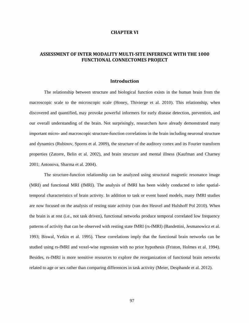
97
CHAPTER VI
ASSESSMENT OF INTER MODALITY MULTI-SITE INFERENCE WITH THE 1000 FUNCTIONAL CONNECTOMES PROJECT
Introduction
The relationship between structure and biological function exists in the human brain from the
macroscopic scale to the microscopic scale (Honey, Thivierge et al. 2010). This relationship, when
discovered and quantified, may provoke powerful informers for early disease detection, prevention, and
our overall understanding of the brain. Not surprisingly, researchers have already demonstrated many
important micro- and macroscopic structure-function correlations in the brain including neuronal structure
and dynamics (Rubinov, Sporns et al. 2009), the structure of the auditory cortex and its Fourier transform
properties (Zatorre, Belin et al. 2002), and brain structure and mental illness (Kaufman and Charney
2001; Antonova, Sharma et al. 2004).
The structure-function relationship can be analyzed using structural magnetic resonance image
(MRI) and functional MRI (fMRI). The analysis of fMRI has been widely conducted to infer spatial-
temporal characteristics of brain activity. In addition to task or event based models, many fMRI studies
are now focused on the analysis of resting state activity (van den Heuvel and Hulshoff Pol 2010). When
the brain is at rest (i.e., not task driven), functional networks produce temporal correlated low frequency
patterns of activity that can be observed with resting state fMRI (rs-fMRI) (Bandettini, Jesmanowicz et al.
1993; Biswal, Yetkin et al. 1995). These correlations imply that the functional brain networks can be
studied using rs-fMRI and voxel-wise regression with no prior hypothesis (Friston, Holmes et al. 1994).
Besides, rs-fMRI is more sensitive resources to explore the reorganization of functional brain networks
related to age or sex rather than comparing differences in task activity (Meier, Desphande et al. 2012).

98
Recently, various brain imaging studies have been conducted in institutes over the world. With
these structural and functional brain MRI studies, a data sharing strategy is badly needed. The idea of
sharing data was proposed over a decade ago with objective of enabling investigators to confirm and
extend the findings of published studies and facilitating discovery science approaches (Van Horn, Grethe
et al. 2001; Van Horn and Gazzaniga 2002; Van Horn, Grafton et al. 2004). Accordingly, the 1000
Functional Connectomes Project was formed in 2009 to aggregate existing rs-fMRI data from
collaborating centers throughout the world (http://www.nitrc.org/projects/fcon_1000/). An initial
demonstration of the feasibility of data pooling and data exploration across centers with the aggregate rs-
fMRI dataset has been published in (Biswal, Mennes et al. 2010). To date, there are over 30 institutes
involved in this study and over 1000 subjects are scanned. The project has proven successful towards
sharing multi-scale data (Mennes, Biswal et al. 2012). With this database, researchers have discovered
complex functional brain networks and the covariates related reorganizations in the human brain
(Rubinov and Sporns 2011; Tomasi and Volkow 2011; Meier, Desphande et al. 2012).
Combining brain image projects together is a powerful idea that provides ―big data‖ sets across
large population and multi-modality brain images. The variance in functional connectivity across
individuals and studies has been studied and characterized (Yan, Craddock et al. 2013). However, how to
combine large scale studies from various sites in a reasonable way is still a challenging problem. Mega-
analysis and meta-analysis are two powerful methods in analyzing multi-site studies (Jahanshad,
Kochunov et al. 2013). Mega-analysis is a fixed-effects analysis that allows pooling the raw information
from individual subject to increase statistical power while maintaining consistent quality control (Serretti,
Cusin et al. 2006; Ripke, Wray et al. 2013). The meta-analysis can be used as a random-effects model that
accounts both the between-site and within-site variability (Etkin and Wager 2007; Seifuddin, Mahon et al.
2012). Herein, we characterized mega- and meta-analysis methods with structure function relationships
inference on the 1000 functional connectomes data.

99
Theory
Mega-Analysis
Mega-analysis jointly analyzes all studies by combining all data together and fits a single model.
This method is a fixed effect model that can fit a model on all data on hand ignoring the between site
variability. It can be described in a general linear model (GLM) treating the factor sites as other
regressors:
(6.1)
In this GLM, the first column of the design matrix is the overall intercept, the are the site
factors for site , and the are other regressors.
The existence of the site difference can be tested using F-test. The null hypothesis is:
which equals to
[
] (6.2)
With this equation we can generate a reduced model assuming the null hypothesis is true, and the F-
statistics can be calculated from the reduced model and the full model.
The significant effects of each covariate can be tested using t-tests.
Meta-Analysis
Meta-analysis can be used to summarize the coefficients from individual site studies (van
Houwelingen, Arends et al. 2002; Becker and Wu 2007). There are fixed effects model and mixed effects
model in meta-analysis ignoring or accounting the site variability respectively (Konstantopoulos 2006).
Here, we focus on the mixed effects model in meta-analysis. Considering each site study to be an
independent random sample from a normal population, we have

100
( )
( )
(6.3)
where is the coefficient for regressor in site , is an estimation of , is the mean coefficient
for regressor of the population. is the within-site variance and represents the between-site
variance.
To test the existence of the site difference on each covariate, the null hypothesis is:
which equals to test the significance of the between-site variance . It can be tested using chi-square
test (Hedges and Pigott 2004; Konstantopoulos 2006).
∑ ( )
∑
∑
(6.4)
where . Under the null hypothesis, follows chi-square distribution with K-1 degrees of
freedom (K is the number of sites).
The significance of the covariate effects can be tested using t-test. In the mixed effects model, the
generalized coefficients are:
∑
∑
(6.5)
where is an estimation of accounting the within-site and between-site variability. The between site
variance can be estimated as:
[
] ∑
∑
∑ (6.6)
The variance of this estimation is:

101
( ) (∑
)
(6.7)
With the mean and variance estimation, we can test the significance of the coefficient by
calculating its t-value. The theory of mega-analysis and meta-analysis are illustrated in Figure 6.1.
An alternatively way of combining statistics is to fit a second level analysis and estimate the
mean effect. However, this approach assumes the variance of the estimated covariates for every site are
the same, i.e., are the same for each . This assumption can hold true for a group study, where every
subject are scanned using the same scanner and the same parameters, but it is not reasonable for different
site studies. The property of accounting both the between-site variance and different within-site variance
makes meta-analysis a very important statistical method in multi-site studies.
Data Quality Assessment
Before statistical analysis, the MRI data must go through pre-processing steps, at least including
Figure 6.1 Model of mega-analysis and meta-analysis. The left side shows the general linear model for the mega-
analysis. The covariates are estimated from regression estimation. The right side shows the framework for meta-
analysis. The covariates are estimated for each site, then they are combined to calculate a final estimation.

102
registration to the same place in the same coordinate system. Since this is a very large scale study, it is
possible that the registration methods failed on some data. Principle component analysis (PCA) may be
used for semi-automatic data quality assessment. Assuming the large variances across an image represent
signals and small variances correspond to noise, PCA can be used for pattern recognition (Turk and
Pentland 1991), manifold learning (Gerber, Tasdizen et al. 2010), and noise reduction (Thomas,
Harshman et al. 2002). It is impossible to view all images together with thousands of voxels in each
image in a large scale study; therefore, we used PCA for dimensionality reduction and explored the
mapped data to find out possible outliers. Specifically, in order to assess the data quality after pre-
processing, we performed PCA on all pre-processed images, and displayed the projection of the data in
two dimensions.
Methods and Results
Data Quality
Within the 1000 Functional Connectome Project, studies conducted in the same center may be
different using different imaging parameters. We considered the images acquired under the same
parameters in the same center as one site study. All the data we used here are from normal ―healthy‖
people, and we only analyzed the data where the age and sex information are available and the resting
state fMRI are acquired for the whole brain. These data information are listed in Table 6.1.
The structural brain MRI images were studied through voxel-based morphometry (Ashburner and
Friston 2000) analyzing the local concentration of gray matter changes. The structural images were skull
stripped by the releasing center. Prior to statistical analysis, the skull stripped structure images were
segmented, normalized to MNI-space, and smoothed (8mm Gaussian kernel) using VBM8 (University of
Jena, Department of Psychiatry, Germany) and SPM8 (University College London, UK). After these pre-

103
processing steps, we got the gray matter (GM) density maps for each subject, which were used for
statistical analysis.
To assess the quality of the normalized GM maps, we performed PCA on the middle axial slice
and on the whole brain within the brain mask for all subjects. When doing PCA on the middle slice, the
voxels outside the brain mask are not excluded, because we need to account the shape of the registered
brain. On the whole brain data assessment, we applied a template brain mask in the MNI-space from
SPM8 and performed PCA on the voxels within the brain mask. We used a template brain mask is
Table 6.1. Data from 1000 Functional Connectome Project
ID Center PI N Parameters
1 Ann Arbor Monk, C.S./ Seidler,
R.D./ Peltier, S.J.
25 22M/3F, ages: 13-40, TR=2, slices=40, timepoints=295
2 Atlanta Mayberg, H.S. 28 13M/15F, ages: 22-57, TR=2, slices=20, timepoints=205
3 Baltimore Pekar, J.J./
Mostofsky, S.H.
23 8M/15F, ages: 20-40, TR=2.5, slices=47, timepoints=124
4 Bangor Colcombe, S. 20 20M/0F, ages: 19-38, TR=2, slices=34, timepoints=265
5 Beijing Zang, Y.F. 198 76M/122F, ages: 18-26, TR=2, slices=33, timepoints=225
6 Berlin Margulies, D. 26 13M/13F, ages: 23-44, TR=2.3, slices=34, timepoints=195
7 Cambridge Buckner, R.L. 198 75M/123F, ages: 18-30, TR=3, slices=47, timepoints=119
8 Cleveland Lowe, M.J. 31 11M/20F, ages: 24-60, TR=2.8, slices=31, timepoints=127
9 Dallas Rypma, B. 24 12M/12F, ages: 20-71, TR=2, slices=36, timepoints=115
10 ICBM Evans, A.C. 86 41M/45F, ages: 19-85, TR=2, slices=23, timepoints=128
11 Leiden Rombouts, S.A.R.B. 12 12M/0F, ages: 20-27, TR=2.18, slices=38, timepoints=215
12 Leiden Rombouts, S.A.R.B. 19 11M/8F, ages: 18-28, TR=2.2, slices=38, timepoints=215
13 Leipzig Villringer, A. 37 16M/21F, ages: 20-42, TR=2.3, slices=34, timepoints=195
14 Milwaukee Li, S.J. 46 15M/31F, ages: 44-65, TR=2, slices=64, timepoints=175
15 Munchen Sorg, C./Riedl, V. 16 10M/6F, ages: 63-73, TR=3, slices=33, timepoints=72
16 Newark Biswal, B. 19 9M/10F, ages: 21-39, TR=2, slices=32, timepoints=135
17 New Haven Hampson, M 19 10M/9F, ages: 18-48, TR=1, slices=16, timepoints=249
18 New Haven Hampson, M 16 8M/8F, ages: 18-42, TR=1.5, slices=22, timepoints=181
19 New York Milham, M.P./
Castellanos,F.X.
84 43M/41F, ages: 7-49, TR=2, slices=39, timepoints=192
20 New York Milham, M.P./
Castellanos,F.X.
20 8M/12F, ages: 18-46, TR=2, slices=33, timepoints=175
21 Orangeburg Hoptman, M. 20 15M/5F, ages: 20-55, TR=2, slices=22, timepoints=165
22 Oulu Kiviniemi, V.J./
Veijiola, J.
103 37M/66F, ages: 20-23, TR=1.8, slices=28, timepoints=245
23 Oxford Smith, S.M./
Mackay, C.
22 12M/10F, ages: 20-35, TR=2, slices=34, timepoints=175
24 Palo Alto Greicius, M. 17 2M/15F, ages: 22-46, TR=2, slices=29, timepoints=235
25 Pittsburgh Siegle, G. 17 10M/7F, ages: 25-54, TR=1.5, slices=29, timepoints=275
26 Queensland McMahon, K. 19 11M/8F, ages: 20-34, TR=2.1, slices=36, timepoints=190
27 Saint Louis Schlaggar, B./
Petersen, S.
31 14M/17F, ages: 21-29, TR=2.5, slices=32, timepoints=127
104
because the whole brain image size is too large and we already assessed the brain shape on the middle
slice. The ratios of the sum of the eigenvalues are plotted in Figure 6.2. To display the all images
together, we plotted the projection of the data to the first two dimensions. One slice of corresponding GM
map is shown on some selected subjects. Because we have a lot of observations and very high
dimensions, the mapped data on the first two dimensions may not provide enough information. To
incorporate the information of more eigenvectors, we viewed the reconstruction errors using these
eigenvectors. Because over 50% percent variances can be represented in the first 20 eigenvectors, we
explored the reconstruction errors using the first 10 eigenvectors. The choice of the number of
eigenvectors is an art that needs further analysis, but it is not our focus here. Here we just chose an
arbitrary number that not include eigenvectors corresponding small eigenvalues, which correspond to
image noise, and showed how well the data can be reconstructed. The reconstruction errors are also
Figure 6.2 PCA results on smoothed Gray Matter density maps. The first row shows PCA results on the middle
slice across all subjects without applying brain mask. The second row shows the PCA results on the whole brain
within the template brain mask. The left column displays eigenvalue ratio, the middle column are mapped data on
the first two dimensions, and the right column are the reconstruction errors using 10 eigenvectors. The red circle
indicates some obvious outliers.

105
displayed in Figure 6.2 with one slice of GM map on selected subjects.
For the rs-fMRI data, the first 5 time points of each time series were discarded when releasing.
The remaining time series were pre-processed using SPM8. The pre-processing steps include temporal
realignment, spatially normalized to MNI space, spatially smoothed with an 8 mm FWHM Gaussian
kernel, and low pass filtered at 0.1 Hz using a Chebychev Type II filter. We did not do slice timing
correction is because the slice order information are not available for every site study.
The pre-processed fMRI data are also underwent PCA analysis on the middle slice and the whole
brain within the brain mask. The PCA analysis results are shown in Figure 6.3.
From these plots and the representing images of the PCA results, we can easily detect outliers as
indicated in Figure 6.2 and Figure 6.3. We explored subjects closed to these outliers and found that most
Figure 6.3 PCA results on pre-processed fMRI images. The first row shows PCA results on the middle slice
across all subjects without applying brain mask. The second row shows the PCA results on the whole brain within
the template brain mask. The left column displays eigenvalue ratio, the middle column are mapped data on the
first two dimensions, and the right column are the reconstruction errors using 10 eigenvectors. The red circle
indicates some obvious outliers.

106
fMRI data from site Atlanta and half data from ICBM are missing regions after normalization. So we
excluded these data some other obvious outliers from other sites. After the data quality assessment, we
used 1086 subjects from 26 sites in the following statistical analysis. Notice that we only applied a typical
and simple pre-processing pipeline with algorithms implemented in SPM8 and VBM8. A better
registration algorithm may provide better results that some bad observations here become acceptable.
Improving data quality is not our focus here; instead, our aim is to show a method that can make the
assessment of the data quality in a large scale study easier and demonstrate that we are able to do further
statistical analysis with these acceptable data.
Multi-site Inference on Gray Matter
The significance of the site difference is explored in the gray matter density maps. The age and
sex related changes have been proved in the gray matter (Chen, Sachdev et al. 2007; Wellington, Bilder et
al. 2013). To account for their influence in the site effects analysis, we fitted a GLM on smoothed gray
matter density maps adjusted for covariates of age, age2, sex, and age×sex. The analyses are performed
using SPM8 using an implicit mask.
The GLM for mega-analysis is:
(6.8)
The positive effects of the mean and every other covariate are tested using one-sided T-test, and the effect
of the site difference is tested using F-test.
In meta-analysis, we applied a GLM model for each site then generalized the estimated statistics.
The GLM for each site is:
(6.9)
From the data information we can see that there are two sites are unisex studies, so the sex and age×sex
covariates are not in the two studies. When we combine the coefficients for sex and age×sex, we only
have 24 sites while other statistics are combined using 26 sites. The effects of the combined statistics are

107
tested using one sided T-test to explore the positive relationship. The effect of the site difference is tested
using Chi-squared test.
The results of the mega-analysis and the meta-analysis are shown in Figure 6.4 and Figure 6.5.
Figure 6.4 shows the significant positive mean effect and the significant site difference under the family
wise error (FWE) correction threshold at p < 0.05. The FWE p-value threshold for each voxel is
calculated based on the smoothness estimation of the full width at half maximum (FWHM). Although this
parameter is different for each sited study in the meta-analysis, they are not very different. Since we used
the same Gaussian kernel in the gray matter smoothness for every image, we used the mean value of the
FWHM over all sites for the FWE correction in meta-analysis. The results of the significance can be
viewed on a glass brain, which is the significance map projected into three dimensions. Here we showed
one dimension of the glass brain with one slice of the significant t-map (t-value exceeds the significant
threshold) overlaid with the corresponding smoothed GM slice. The positive effects of age and sex are
Figure 6.4 Mega- and Meta-analysis results of site difference and mean effect on smoothed GM maps. The top
row displays the results in one dimension of a glass brain. The bottom row displays the t-value of the significant
voxels overlaid with one slice GM map. The left two columns are results from mega-analysis and the right two
columns are results from meta-analysis.

108
much less significant that few voxels show significance under the FWE corrected p-value threshold at
0.05. We showed the significant results for age, age2, sex, and age×sex coefficients under uncorrected p-
value threshold at p < 0.001.
The site difference and mean effect from mega-analysis and meta-analysis are similar and exist
almost everywhere. The significant site difference region from meta-analysis seems a little larger than
from mega-analysis, noting that the resulting brain mask from mega-analysis and meta-analysis are the
same. The significant regions of age, age2, sex, and age×sex effects from mega-analysis are larger than
from meta-analysis. This may due to the fact that mega-analysis is a fixed effect analysis ignoring the
between-site variance while meta-analysis is a mixed effect analysis accounting the between-site
variability. Thus, the same estimated coefficient will have higher t-value from mega-analysis than from
meta-analysis.
To explore the relationship of the mega- and meta-analysis, we analyzed the agreement of their
statistical maps and significant maps. Their linear relationship is shown by regressing the statistical value
from the meta-analysis on the statistical value from the mega-analysis. The correlations on the statistical
maps and the Dice coefficients on the displayed significance maps (FWE p < 0.05 for site difference and
Figure 6.5 Mega-analysis and Meta-analysis results of age, age2, sex, and age×sex effects on smoothed GM
maps. The top row shows the results from mega-analysis and the bottom row displays the results from meta-
analysis. For each covariate effect, one dimension of the glasss brain and one slice of the significant t-value map
overlaid with the GM map are shown.

109
mean effect, uncorrected p < 0.001 for other covariates) are calculated. The results are shown in Figure
6.6.
The relationship results show that the correlation of the mega- and meta-analysis on the site
difference is very high. The correlations for other effects are much lower but all exceed 0.4, and in most
cases the scale of the statistical value from mega-analysis are larger than the statistical value from meta-
analysis. When it comes to the significance map, the Dice coefficients are high for all statistical tests. It
reaches 1 for the positive mean effect test because the mean effects are significant everywhere within the
brain mask under mega- or meta-analysis.
Figure 6.6 Relationship of the mega- and meta-analysis results on smoothed GM maps. The x-axis represents the
statistical value from the mega-analysis (F-statistics for site difference, T-statistics for covariates). The y-axis
represents the statistical value from the meta-analysis (Chi-squared statistics for site difference, T-statistics for
covariates). The blue dots are voxels within the brain mask, and the black lines are linear regression line
regressing the meta-analysis results on the mega-analysis results. The r value shown on the plots are the
correlation value and the Dice represents the Dice coefficient of the significance maps.

110
Multi-site Inference on Functional Connectivity
The low frequency correlation of the blood flow under rest can be tested using a seed model with
rs-fMRI. In the seed model functional connectivity analysis, a seed region is selected and its connectivity
to the rest of the brain is analyzed. The selection of the seed region is different for different purpose and is
based on the specific clinical questions. The hippocampus network has been proved to be related to
memories in human and in animals (Neves, Cooke et al. 2008; Takashima, Nieuwenhuis et al. 2009) and
the age effects were demonstrated in the shape analysis of hippocampus in normal people (Xu, Valentino
et al. 2008). Here we studied the site effects on the hippocampus functional connectivity network
accounting the covariates of age, age2, sex, and age×sex using mega- and meta-analysis. The left
hippocampus (LH) is selected as the seed region using the atlas in the WFUpickatlab toolbox
(fmri.wfubmc.edu/software/PickAtlas). For each pre-processed fMRI, we calculated the average image
intensity across all voxels in the LH to get the seed time series for the connectivity analysis. The six
estimated motion parameters from realignment estimation were used as confounds. After the functional
connectivity analysis we got a t-map of the LH functional connectivity for each subject.
We used the model described in equation (6.8) for mega-analysis and the model in equation (6.9)
for each site studies in meta-analysis. The mean and other covariate effects were tested using one-sided T-
test to explore the positive relationships and the site difference was tested using F-test and Chi-squared
test for mega- and meta-analysis respectively. The results are shown in Figure 6.7 and Figure 6.8 on one
dimension of the glass brain and one slice of the significant t-map overlaid with the corresponding
smoothed gray matter image. Figure 6.7 shows the significant mean effect and the site difference under
the FWE correction threshold at p < 0.05. Since both the left and the right hippocampus are in the
hippocampus network related to memories, we can expect the LH functional connectivity map is
significant on the right hippocampus. The mean effect of the functional connectivity maps analysis is in
fact a mean LH functional connectivity map acquired from a group analysis. From Figure 6.7 we can see
that the LH has the highest mean effect t-value for both mega- and meta-analysis, this is because we
calculated the seed time course from this region. Besides the left hippocampus, the right hippocampus has

111
the highest mean effect t-value, which agrees with our expectation. The site difference seems existing
everywhere, which agrees with the GM analysis.
Figure 6.7 Mega- and Meta-analysis results of site difference and mean effect on LH functional connectivity
maps. The top row displays the results in one dimension of a glass brain. The bottom row displays one slice of
the significant t-value map overlaid with the GM map. The left two columns are results from mega-analysis and
the right two columns are results from meta-analysis.
Figure 6.8 Mega- and Meta-analysis results of age, age2, sex, and age×sex effects on LH functional connectivity
maps. The top row shows the results from mega-analysis and the bottom row shows the results from meta-
analysis. For each covariate effect, one dimension of the glasss brain and one slice of the significant t-value map
overlaid with the GM map are shown. There is no significant age effect from meta-analysis and not shown here.

112
For age, age2, sex, and age×sex effects, there are few voxels significant under FWE corrected
threshold at p < 0.05 so we show the significant results under uncorrected p-value threshold at p < 0.001
in Figure 6.8. There is no significant age effect under the uncorrected p < 0.001 in meta-analysis and
nothing was shown. For other covariates effect, the number of significant voxels from the meta-analysis is
much smaller than from the mega-analysis. In the mega-analysis results, there are a lot of voxels at the
edge of the brain show significance for the age2 and sex effect. This may because that the covariate has an
effect on the shape of the brain some subjects have value on these voxels while subjects not.
The relationships of the mega- and meta-analysis are displayed in Figure 6.9. When we
performed the analysis we did not provide any explicit brain mask, but only used the implicit brain mask
calculated by SPM8. After analysis, SPM8 will output a brain mask. Here the brain mask from the mega-
Figure 6.9 Relationship of the results from mega- and meta-analysis on LH functional connectivity maps. The x-
axis represents the statistical value from the mega-analysis (F-statistics for site difference, T-statistics for
covariates). The y-axis represents the statistical value from the meta-analysis (Chi-squared statistics for site
difference, T-statistics for covariates). The blue dots are voxels within the brain mask, and the black lines are
linear regression line regressing the meta-analysis statistical value on the mega-analysis statistical value. The r
value shown on the plots are the correlation value and the Dice is the Dice coefficient of the significance maps.
113
analysis is larger than the brain mask calculated from the meta-analysis, thus we explored their
relationship within the brain mask calculating from the meta-analysis. The correlations of the mega- and
meta-analysis are not high for each statistical test but the Dice coefficients are high for all tests.
Multi-site Inference on Structure-Function Relationships
In recent years, the structure function relationships have attracted more and more attentions in
understanding how the human brain works. With the gray matter density maps and functional
connectivity maps it is easy to assess their relationship using Biological Parametric Mapping (BPM)
(Casanova, Srikanth et al. 2007). Here we use BPM to explore the question that how the gray matter
density maps explain the left hippocampus connectivity maps. We analyzed their relationship using
similar GLMs described in equation (6.8) and equation (6.9) for mega- and meta-analysis. The LH
functional connectivity maps were analyzed as regressand and the GM maps were included as another
regressor. BPM enables the analysis of multi-modality brain images; however, BPM is sensitive to
outliers. This problem can be overcome through robust regression, the robust version of BPM (rBPM) has
been introduced and demonstrated to be reliable to outliers (Yang, Beason-Held et al. 2011). Although
obvious outliers are discarded in the data quality assessment, it is very possible some outlier observations
are included in the analysis. It is hardly to discard all problematic data automatically. Besides, the mis-
registrations in the voxel level are hard to see even if we manually check every registered image.
Therefore, the reliability of rBPM to outliers will be very helpful in the structure function relationship
studies. Herein, we analyzed the relationships between the smoothed GM maps and LH functional
connectivity maps using BPM and rBPM.
The significance of the mean effect and the GM effect are shown in Figure 6.10. Other covariates
effects are small compared to these two effects and not shown here. The significance maps are calculated
under FWE corrected p-value threshold at p < 0.05. One dimension of the glass brain and one slice of the
significant t-map overlaid with the corresponding GM map are shown. In the BPM and rBPM analysis,
we did not provide any explicit brain mask but an implicit brain mask was calculated based on the number

114
of nonzero observations. Because the brain mask calculated from the meta-analysis are much smaller than
from the mega-analysis, a lot of significant mean effect voxels in the mega-analysis are missing in the
meta-analysis. The left and right hippocampus are the most significant mean effect regions in both mega-
and meta-analysis, which is consistent with the functional connectivity analysis. Most of the significant
regions from BPM and rBPM analysis are similar but with some difference.
The comparison of the mega- and meta-analysis results on the structure function relationship
analysis using BPM and rBPM are shown in Figure 6.11. The t-values for each coefficient from the
Figure 6.10 Mega- and Meta-analysis results using BPM and rBPM model. The first two rows are the results
using BPM and the last two rows are the results using rBPM. The left two columns are the results from mega-
analysis and the right two columns are the results from meta-analysis.

115
mega-analysis are plotted versus the t-values from the meta-analysis within the brain mask calculating in
the meta-analysis. The correlations of the mean effect and the GM effect from mega- and meta-analysis
are higher than 0.5 while the correlations of other effects are low. The Dice coefficients are high for all
effects (under FWE corrected p-value at p < 0.05 for mean and GM effects and uncorrected p-value at p <
0.001 for other effects). An interesting finding is that the correlations of mega- and meta-analysis results
using rBPM are all slightly bigger than the corresponding correlations using BPM.
Figure 6.11 Relationship of the results from mega- and meta-analysis on structure function relationship analysis.
The left two columns show the results using BPM and the right two columns show the results using rBPM. For
each regressor effect, the t-value from mega- and meta-analysis are plotted (blue dots). The black lines show the
regression of t-value from mega-analysis on the t-value from meta-analysis. The r value is the correlation of the
mega- and meta-analysis and the Dice is the Dice coefficient of their significance maps (FWE threshold at p <
0.05 for mean and GM effect, uncorrected p < 0.001 for other effects).

116
Discussion
As the sharing of multi-site studies succeeding in the genetics analysis (Mailman, Feolo et al.
2007; Jahanshad, Kochunov et al. 2013), large scale data sharing has attracted more and more attentions
in the neuroimaging community (Mennes, Biswal et al. 2012). Besides the concern of protecting privacy
and data organization, the challenge of handling rich datasets in an orderly and efficient way has
increased. Our work presented here provides a semi-automatic method for assessing the pre-processed
data quality, proves the feasibility of analyzing multi-site data using mega- and meta-analysis, and
demonstrates the usefulness of robust BPM in large scale structure function relationship studies. The data
qualities are varied from subject to subject as well as site to site. After dimensionality reduction using
PCA, the failed registered brain images are easily to see and can be removed in following statistical
analysis. Although there may still exist some subtle outliers, the data should be acceptable for large scale
statistical analysis. Besides, the rBPM is reliable to outliers when the number of failed registered images
is small compared to the whole dataset.
Mega-analysis and meta-analysis are two typical widely used methods in combining statistics
from multi-site data. The mega-analysis is a fixed effect model ignoring the between-site variance that
can be described in a simple GLM. The meta-analysis described here is a mixed effect model accounting
the between-site variance that can be used for generalizing inference. From our results, we can see that
the site difference exist almost everywhere in both the GM maps and the LH functional connectivity
maps. According to this discovery, it seems more reasonable to account the between-site variability in
analysis. When it comes to the coefficient inference, the mega-analysis always shows more significance
than the meta-analysis. This proves that by accounting the between-site variance the meta-analysis can
better control the type I error than the mega-analysis while may lose the power of detection. The
correlations between mega- and meta-analysis in our study are high if there are large significant regions in
the brain (e.g., site difference, mean effect, and GM effect) but become low if not (e.g., age effect and sex
effect). The Dice coefficients, however, stays high under FWE corrected p-value threshold at p < 0.05 or

117
uncorrected p-value threshold at p < 0.001. These results prove enough agreement between mega-analysis
and meta-analysis that the statistical inferences are reliable.
The BPM and rBPM can be used with the mega- and meta-analysis for large scale structure
function relationship studies. Our empirical results show higher correlation of the mega- and meta-
analysis using rBPM than using BPM, which agrees with its reliability to outliers. The mis-registration
problems are hard to address or identify for all data in a large database. With acceptable number of
outliers, we are still able to draw inference using multi-site data. The work here proves that with mega-
and meta-analysis, we can not only assess the within-modality relationship but also reliable between
modality relationships using large scale datasets.
In this study, we only applied typical pre-processing pipelines implemented in SPM, other
registration methods or additional process may result in interesting findings but beyond the scope of this
paper. The age and sex covariates were included in our three study models because they are common
findings associated with brain changes, but we did not aim to hypothesize or prove any age or sex effects.
In the functional connectivity analysis, the selection of the seed region will affect results, but here we
were not interested in finding or validating any hypothesis. Instead, we aim to show an example of multi-
site studies on functional connectivity analysis for mega- and meta-analysis exposition. The left
hippocampus was defined as the seed region because the hippocampus networks are widely studied and
the age effects have been studied on this region, but other connectivity maps can be studied here. The goal
of this paper is to prove that (1) the huge significance of site effect should encourage extreme caution and
(2) the increased power with mega- over meta- analysis show encourage full data sharing rather than
summary statistics.

118
CHAPTER VII
CONCLUSIONS AND FUTURE WORK
Summary
This dissertation concerns the robustness and realistic considerations of statistical models in
human brain mapping within the general linear model (GLM) framework. The GLM has been widely
accepted in the neuroimaging community, but problems occur as these approaches are applied to larger,
multi-modal, and/or heterogeneous datasets. We focus on addressing limitations of the GLM within
multi-modality brain image analysis and functional connectivity analysis. In Chapter II, we provide a
robust model that is reliable to outliers in the structure-function relationships analysis. Chapter III
further addressed issues in the structure-function relationships analysis and introduced models that can
account for random regressors. The methods proposed in Chapter II and Chapter III were implemented
in the biological parametric mapping (BPM) framework. We collaborated with neuroscientists on
empirical clinical applications. One clinical application is the study of the relationship between resting
state functional connectivity and gray matter concentration in temporal lobe epilepsy (Holmes, Yang et al.
2013). Another application is for the Baltimore Longitudinal Study of Aging exploring the relationships
between distribution volume ratio and cerebral blood flow (Sojkova, Goh et al. 2013/09).
With the availability of alternative statistical approaches for testing the same fundamental
hypotheses, deciding among statistical methods becomes a problem unto itself. Traditionally,
methodological decisions have been based on asymptotic theory and simulation experiments; yet, such
studies do not provide specific information regarding the appropriateness of a method for any individual
dataset. We applied new innovations in finite sample statistics to provide quantitative information on the
relative performance of individual (non-repeated) fMRI datasets. The SIMulation and EXtrapolation
(SIMEX) approach can estimate the bias of an estimator on finite samples base on the notion that the

119
expected value of an estimator diverges smoothly with increasing noise levels, therefore, the mean degree
of corruption can be estimated by extrapolating a trend of divergence when synthetic noise is added to
empirical data and randomized data subsampling. Motivated by this theory we proposed a quantitative
evaluation method that can compare statistical inference models on empirical resting state fMRI data
(Chapter IV). For single subject studies, ordinary least squares method outperforms robust regression on
most clean 3T data while robust regression is better on some 7T data which may have relatively higher
physiological noise. As is expected, no one statistical approach dominates, and selection of methods
remains a nuanced decision. Yet, we have created a quantitative method to guide domain experts.
In functional connectivity studies, the time series are correlated, which has been routinely
considered in statistical GLM models. However, very few models can consider the temporal correlations
and the spatial correlations simultaneously in estimation. Ignoring spatial correlations may under-estimate
the standard deviations that will increase false positive rates. In Chapter V, we extended a ROI-based
spatio-spectral mixed-effects model to the whole brain resting state functional connectivity analysis. We
also applied the ideas in this model to the voxel-wise models within the statistical parametric mapping
(SPM) framework to take both the spatial correlations and temporal correlations into account. The
benefits of the ROI-based spatio-spectral and voxel-wise spatio-temporal models for fMRI connectivity
analysis were demonstrated in theory and simulations. For empirical studies, this work needs further
development and characterize group level analysis for more typical study designs. Moreover, the
connectivity structure estimated by this approach is potentially ground breaking, but a deeper analysis of
estimatable properties and biological considerations is warranted.
Data sharing has fostered democratization of interpretation of medical images and allowed
exploration by a greater pool of scientists. These efforts are typified by the 1000 functional connectomes
project. In contrast to traditional small-scale studies, imaging protocols differ from site to site in the
public data resources. Hence, there are substantial concerns regarding how one should perform
―federated‖ studies – e.g., should summary measures be combined (―meta-analysis‖) or should all
imaging data be analyzed simultaneously (―mega-analysis‖). We studied the site effects using mega- and

120
meta-analysis with 1000 functional connectomes project in Chapter VI. The results show substantial and
significant site difference over the whole brain and much strong effects observed with mega- analysis
opposed to meta-analysis. While the underlying causes of the site difference are relatively unexplored,
demonstration of its existence encourages cautions of modeling site effects for multi-site studies. Further
efforts are needed to investigate compensation for site difference (e.g., more robust image processing and
segmentation) and modeling site differences (e.g., linear modulation versus parametric modeling of
acquisition). Nevertheless, the conclusion that sharing of raw data enables more powerful science than
sharing of summary statistics is well-justified.
In the following sections we detail the main results of each contribution.
Reliable Statistical Inference in Multi-modality Brain Image Analysis
Unlike traditional statistical parametric mapping, biological parametric mapping (BPM) can
explain changes in one modality brain image using information from other modality brain images. During
our experiments of structure-function relationship studies, we explored the problems within the traditional
statistical estimation methods in the multi-modality brain image analysis. To lower the sensitivity of BPM
to outliers, we proposed robust regression and non-parametric mapping methods to in inter modality brain
image studies.
Main Results
1. The main difference between inter modality brain image analysis and intra modality brain
image analysis is that the design matrix contains other modality brain image information.
Because of this difference, (1) the possibility of the appearance of outlier increases and (2)
the observation of imaging regressors are not fixed (i.e., should be treated as random
variable).

121
2. We explored possible statistical methods to increase the reliability of BPM analysis: robust
regression and non-parametric mapping. Robust regression can provide reliable estimation by
lowering the influence of possible outlier observations when outlier occurs and at the same
time being 95% efficient if no outliers exist. Non-parametric mapping can be used for
estimation when the Gaussian distribution assumption is not reasonable or the sample size is
small.
3. We demonstrated that the robust and non-parametric models are compatible with the general
linear model framework and multiple comparison correction methods. They are implemented
in the same pipeline as the traditional human brain mapping.
4. We evaluated application of these methods in simulation and explaining the use in empirical
experiments, illustrating the usefulness in the context of BPM and multi-modality image
regression.
5. We released software resources (http://www.nitrc.org/projects/rbpm/) to allow others to use
these tools. These have been downloaded over 200 times (October 2013).
6. Use of the software toolbox was evaluated in two hypothesis-driven studies. In the temporal
lobe epilepsy study, it was used to explore the relationship between gray matter
concentrations and resting functional connectivity (hippocampus and thalamus). In
longitudinal aging study, it was used to explore the relationship between distribution volume
ratio and cerebral blood flow.
Future Work
The robust regression is reliable to outliers, but there are several robust weight functions, which
may result in slightly different inference. The comparison of different robust weight functions can be
studied to set up criteria of choice in empirical use. For more robust analysis, a robust smoothness
estimation method may be useful. Although we can mitigate smoothness concerns by pooling data across

122
images, exploring the influence for post multiple comparisons could provide more accurate corrected p-
value thresholds.
Addressing Random Regressors in Multi-Modality Brain Image Analysis
The multi-modality brain image analysis requires images on images regression, where the
regressors are not fixed value as most traditional models (e.g., age, sex). To more accurately model this
realistic situation and provide accurate estimation, we introduced Model II regression and regression
calibration that can account for the regressors with measurement error.
Main Results
1. We explored statistical models that can account for random regressors in the estimation:
regression calibration and Model II regression. In simulation, we demonstrated that the
regression calibration can better control the type I error and the type II error than ordinary
least squares (OLS) method, but requires replicated measurements of the random regressors.
The Model II regression is also better than OLS by using the measurement error ratio of the
regressors to the regressand and provides symmetric estimations. In empirical studies, the
measurement error ratio can be estimated through signal to noise ratio estimation, which has
been widely studied in the MRI imaging community.
2. We demonstrated these models in the statistical parametric mapping framework, evaluated
their applications in simulation and empirical experiments, and illustrated the usefulness in
the multi-modality image analysis. With empirical data, no ground truth is available, so only
differences between analyses were determined.
3. The extended BPM toolbox provides statistical methods that offer robustness to outliers and
can account for regressors as random variables (http://www.nitrc.org/projects/rbpm/).

123
4. These proposed models can not only be used in raw brain image analysis across multiple
modalities, but also in the analysis of different brain maps. For example, we can explore the
relationship between the structural map and the functional connectivity map or the
relationship between the changes and the baseline. With our work here, structural-functional
hypothesis may be directly assessed.
Future Work
The proposed statistical model addresses the measurement error of the regressors separately, but
does not directly integrate robust regression for outlier exclusion. A further research direction will be
combing these two characteristics in an efficient way. For random regressors, we may work on the
estimation of measurement errors. Accurately estimating the measurement error of the random regressors
will increase the accuracy of the inter modality relationship estimation. Acquiring replicated
measurements is a severe constraint in the neuroimaging community, but there may be special study
designs for which this is an appropriate solution.
Robust Statistics and Empirical Validation in Functional Connectivity Analysis
We present a new technique to compare statistical methods using non-repeated finite samples of
fMRI data. These methods provide the first quantitative data on which to compare potential statistical
models using single datasets. The theoretical motivation is the novelty of SIMEX, which can estimate the
expectation of an estimator on finite samples. Herein, we showed it is possible to compare statistical
methods with finite empirical data where the noise structure is unknown.
Main Results
1. We investigated the model fitting residuals based on two 7T and one 3T protocols. Imaging
slices that passed through regions with peak inhomogeneity problems (e.g., mid-brain

124
acquisitions for the 7T hippocampus) exhibited visually higher degrees of distortion along
with extreme values of kurtosis (a measure of non-Gaussianity). Our early error investigation
showed that artifacts in the 7T fMRI dataset had greater impact on statistical method than the
3T datasets --- such results are anecdotal, but in line with expected scanner performance
given known issues of hardware stability.
2. We implemented the robust regression within the restricted maximum likelihood framework
for resting state fMRI (rs-fMRI) functional connectivity analysis.
3. We proposed a novel approach for quantitatively evaluating statistical inference methods
based on their resilience in the sense of diminishing data. The core theory there is similar to
the SIMEX technique, but instead of adding noise to estimate the bias we diminished data to
estimate the resilience. This approach can evaluate the performance on empirical data where
noise structure or the truth is unknown and it does not require acquisition of additional data.
4. We demonstrated our proposed evaluation approach is consistent with type I error and type II
error in simulation with known truth.
5. The studies confirmed expectations in the limited empirical datasets with known issues.
Compared to OLS, the M-estimator robust regression was not needed for the clean single
subject 3T fMRI analysis but resulted in superior performance metrics for the 7T dataset with
artifacts.
Future Work
Our proposed method is a promising but initial work on comparing statistical inference methods
on empirical data. In empirical experiments, both the true relationship and the noise structure are
unknown. To satisfy the argument when simulation cannot capture empirical features, a comparison
method using empirical data will accelerate the development of statistical models in human brain
mapping and bring in more convincing results.

125
Spatial Temporal Models for Resting State fMRI Analysis
We extended a ROI-based spatio-spectral mixed-effects model for task fMRI analysis to rs-fMRI
connectivity analysis. Our proposed ROI-based spatio-spectral mixed-effects model can take within-ROI
and between-ROI spatial correlations as well as temporal correlations into account simultaneously. To
apply this model to widely used voxel-wise analysis, we proposed a voxel-wise spatio-temporal model
using a sliding window to address the within window spatial correlations as well as temporal correlations
for each voxel.
Main Results
1. We extended a spatio-spectral mixed-effects model for ROI-based resting state fMRI
analysis. We derived an efficient way in estimating spatial correlations and the covariance of
estimated coefficients, which extends the use of this model in the whole brain functional
connectivity analysis. A pipeline of the whole brain ROI-based functional connectivity
analysis using spatio-spectral model was established and demonstrated through simulation
and empirical experiments.
2. We proposed two voxel-wise spatio-temporal models that can account for the spatial
correlations as well as the temporal correlations in rs-fMRI studies. The temporal correlations
are addressed using autoregressive model with restricted maximum likelihood estimation and
the spatial correlations are considered within a sliding window and estimated though
variogram estimation.
3. In simulation, both the ROI-based spatio-spectral model and the voxel-wise spatio-temporal
model prove to work well. Positive spatial correlation may lead to loss of the control of type I
error. The proposed model improves control the type I error in such cases.
4. In empirical studies, because of the low contrast to noise ratio in the resting state fMRI data,
there were no significant inference from ROI-based analysis using tradition or spatio-spectral

126
model. In voxel-wise analysis on an unsmoothed 7T dataset, the significant results from
traditional methods are very noisy while fewer false positive voxels appear using our spatio-
temporal model with voxel-wise test. These results are preliminary and should be considered
inconclusive given the limited context.
Future Work
The spatial-spectral analysis demonstrates a feasible theoretical approach for handling multi-ROI
analyses. The empirical study presented is exploratory and has not demonstrated the clinical/practical
usefulness of this approach. Our proposed models can take the temporal and spatial correlations into
account simultaneously and better control the type I error than traditional models ignoring spatial
correlations in simulations. To translate these methods for clinical applications, we need to combine
statistical results from these models for group analysis and conduct a study of noise sensitivity/specificity.
The voxel-wise spatial-temporal models are interesting re-posing of the estimation problem, but
are relatively unexplored. The window size may affect the results and the choice needs further
justification. A best window size should be able to balance the need of accurate spatial correlations
estimation and the significant size, and an adaptive window for each voxel may be more appropriate.
Such approaches may converge with recent perspective on spatially adaptive smoothing and more
traditional GLM models.
Multi-Site Brain Image Study
We considered study design for multi-site brain mapping using mega- and meta-analysis. Over
1000 structural and resting state functional brain images were pre-processed under a typical pipeline and
the data qualities were accessed using principle component analysis. We explored the site difference
accounting the effects of age and sex as covariates in gray matter (GM) density analysis, functional

127
connectivity analysis, and their relationships analysis. The correlations between mega- and meta-analysis
are established and the differences are explored.
Main Results
1. This research is exploratory. The statistical methods suggest differences across sites, but we
did not specifically seek to explain these differences. Continuing efforts are examining
factors that lead to these site effects.
2. We explored the mega-analysis and the meta-analysis in statistical brain mapping using large
scale data. The difference between mega and meta analysis are due to the fixed effects and
random effects considerations. The mega-analysis is a fixed effects analysis method that can
be explained in a simple general linear model. The meta-analysis can be used as a random
effects analysis to infer generalized conclusions. Their correlations and differences were
established in GM map analysis, left hippocampus functional connectivity map analysis, and
their relationships analysis.
3. We proposed a semi-automatic data quality assessment approach to show possible outliers
using Principle Component Analysis (PCA). After dimensionality reductions using PCA, the
brain imaging data can be viewed together and their reconstruction errors can be evaluated.
Based on a two dimensions view of the pre-processed images and their reconstruction errors
using first ten eigenvectors, we were able to detect outliers and exclude them in the following
statistical analysis.
4. The increased power with mega- over meta-analysis shows encourage of full data sharing
rather than summary statistics.
5. We demonstrated the practical performance of our analysis toolbox software for large-
datasets and multi-site studies.

128
Future Work
In addition to data management and organization, heterogeneous data introduces statistical
challenges for big-data studies. This work focus on studying the existence of site differences using mega-
and meta- inference approaches. However, the reason of the site effects is still unclear that needs further
study. The contribution of our work here is drawing the attention of considering site effects in multi-site
analysis. Another finding of this work is the increased power with mega- over meta-analysis. To explore
more specific neuro-scientific hypotheses, we need to collaborate with neuroscientists in future studies
using multi-site data. Another direction of the future work is improving the data quality assessment
method to provide a quantitative and more accurate justification.
Overall Perspective
The goal of the presented work in this dissertation is to explore the robustness and accuracy in
human brain mapping within a widely used statistical parametric mapping framework. Specifically, we
focused on the multi-modality structural functional brain image analysis and resting state functional
connectivity analysis. We demonstrated that modern statistics can be compatible with general linear
model to provide reliable and accurate estimations. An evaluation method of comparing statistical
inference methods on empirical data was proposed for resting state functional connectivity. For analysis
using multi-site data, mega- and meta-analysis were explored and site differences were discovered. The
statistical methods have shown that the differences between sites are unlikely to have occurred by chance,
but the optimal approaches for compensating for such effects (post hoc or during study design) remains a
challenging problem for the field. The theme of the work presented in this dissertation is from the
perspective of a statistical engineer – i.e., translating statistics into practice (as opposed to statistical
theory or basic science). Our contributions are explorations of appropriate statistical theories in detail for
medical image analysis and the methods proposed were demonstrated in simulations. The presented
empirical studies aim to explain the methods and illustrate how to use them. To gain deeper insight of the

129
application to make our work more biomedically meaningful, we need to work with neuroscientists. To
date, we have collaborated with two neuroscientists for multi-modality brain image analyses; other work
will be applied in the future. We hope the work in this dissertation can attract attention to using
appropriate statistical models in human brain mapping and the toolbox developed here can lead to
interesting clinical research findings.

130
REFERENCES
Afshin-Pour, B., H. Soltanian-Zadeh, et al. (2011). "A mutual information-based metric for evaluation of
fMRI data-processing approaches." Human Brain Mapping 32(5): 699-715.
Altman, D. G. (1991). Practical statistics for medical research, CRC Press.
Antonova, E., T. Sharma, et al. (2004). "The relationship between brain structure and neurocognition in
schizophrenia: a selective review." Schizophr Res 70(2-3): 117-145.
Ashburner, J. and K. J. Friston (1999). "Nonlinear spatial normalization using basis functions." Human
Brain Mapping 7(4): 254-266.
Ashburner, J. and K. J. Friston (2000). "Voxel-based morphometry--the methods." Neuroimage 11(6 Pt
1): 805-821.
Asman, A. J. and B. A. Landman (2012). "Formulating spatially varying performance in the statistical
fusion framework." IEEE Trans Med Imaging 31(6): 1326-1336.
Asman, A. J. and B. A. Landman (2013). "Non-local statistical label fusion for multi-atlas segmentation."
Med Image Anal 17(2): 194-208.
Bandettini, P. A., A. Jesmanowicz, et al. (1993). "Processing strategies for time-course data sets in
functional MRI of the human brain." Magn Reson Med 30(2): 161-173.
Banerjee, S., B. P. Carlin, et al. (2004). Hierarchical modeling and analysis for spatial data. Boca Raton,
Fla., Chapman & Hall/CRC.
Beason-Held, L. L., M. A. Kraut, et al. (2008). "I. Longitudinal changes in aging brain function."
Neurobiol Aging 29(4): 483-496.
Beaton, A. E. and J. W. Tukey (1974). "Fitting of Power-Series, Meaning Polynomials, Illustrated on
Band-Spectroscopic Data." Technometrics 16(2): 147-185.
Becker, B. J. and M. J. Wu (2007). "The synthesis of regression slopes in meta-analysis." Statistical
Science 22(3): 414-429.
Benjamini, Y. and Y. Hochberg (1995). "Controlling the False Discovery Rate - a Practical and Powerful
Approach to Multiple Testing." Journal of the Royal Statistical Society Series B-Methodological
57(1): 289-300.
Benjamini, Y. and D. Yekutieli (2001). "The control of the false discovery rate in multiple testing under
dependency." Annals of Statistics 29(4): 1165-1188.
Biswal, B., F. Z. Yetkin, et al. (1995). "Functional connectivity in the motor cortex of resting human brain
using echo-planar MRI." Magn Reson Med 34(4): 537-541.
Biswal, B. B., M. Mennes, et al. (2010). "Toward discovery science of human brain function." Proc Natl
Acad Sci U S A 107(10): 4734-4739.
Biswal, B. B., J. Van Kylen, et al. (1997). "Simultaneous assessment of flow and BOLD signals in
resting-state functional connectivity maps." NMR Biomed 10(4-5): 165-170.
Bookstein, F. L. (2001). ""Voxel-based morphometry" should not be used with imperfectly registered
images." Neuroimage 14(6): 1454-1462.
Bradley, A. P. (1997). "The use of the area under the roc curve in the evaluation of machine learning
algorithms." Pattern Recognition 30(7): 1145-1159.
Carroll, R. J., H. Kuchenhoff, et al. (1996). "Asymptotics for the SIMEX estimator in nonlinear
measurement error models." Journal of the American Statistical Association 91(433): 242-250.
Carroll, R. J. and D. Ruppert (1996). "The use and misuse of orthogonal regression in linear errors-in-
variables models." American Statistician 50(1): 1-6.
Carroll, R. J., D. Ruppert, et al. (2010). Measurement error in nonlinear models: a modern perspective,
CRC press.
Casanova, R., R. Srikanth, et al. (2007). "Biological parametric mapping: A statistical toolbox for
multimodality brain image analysis." Neuroimage 34(1): 137-143.

131
Chen, C. (2002). "Robust regression and outlier detection with the ROBUSTREG procedure." SUGI
Paper(265-27).
Chen, X., P. S. Sachdev, et al. (2007). "Sex differences in regional gray matter in healthy individuals aged
44-48 years: a voxel-based morphometric study." Neuroimage 36(3): 691-699.
Cook, J. R. and L. A. Stefanski (1994). "Simulation-Extrapolation Estimation in Parametric Measurement
Error Models." Journal of the American Statistical Association 89(428): 1314-1328.
Cordes, D., V. M. Haughton, et al. (2000). "Mapping functionally related regions of brain with functional
connectivity MR imaging." AJNR Am J Neuroradiol 21(9): 1636-1644.
Delong, E. R., D. M. Delong, et al. (1988). "Comparing the Areas under 2 or More Correlated Receiver
Operating Characteristic Curves - a Nonparametric Approach." Biometrics 44(3): 837-845.
Deming, W. E. (1943). "Statistical adjustment of data."
Diedrichsen, J. and R. Shadmehr (2005). "Detecting and adjusting for artifacts in fMRI time series data."
Neuroimage 27(3): 624-634.
Dubin, R. A. (1988). "Estimation of regression coefficients in the presence of spatially autocorrelated
error terms." The Review of Economics and Statistics: 466-474.
Dumouchel, W. and F. O'Brien (1991). "Integrating a robust option into a multiple regression computing
environment." Institute for Mathematics and Its Applications 36: 41.
Etkin, A. and T. D. Wager (2007). "Functional neuroimaging of anxiety: a meta-analysis of emotional
processing in PTSD, social anxiety disorder, and specific phobia." Am J Psychiatry 164(10):
1476-1488.
Fisher, R. A. (1925). "Applications of Student's Distribution." Metron 5: 90-104.
Fox, J. (2002). An R and S-Plus companion to applied regression, Sage.
Fox, P. T., M. A. Mintun, et al. (1986). "Mapping human visual cortex with positron emission
tomography." Nature 323(6091): 806-809.
Friston, K., P. Jezzard, et al. (1994). "Analysis of functional MRI time‐series." Human Brain Mapping
1(2): 153-171.
Friston, K. J., J. T. Ashburner, et al. (2007). Statistical Parametric Mapping: The Analysis of Functional
Brain Images, Academic Press.
Friston, K. J., C. D. Frith, et al. (1990). "The Relationship between Global and Local Changes in Pet
Scans." Journal of Cerebral Blood Flow and Metabolism 10(4): 458-466.
Friston, K. J., C. D. Frith, et al. (1991). "Comparing functional (PET) images: the assessment of
significant change." J Cereb Blood Flow Metab 11(4): 690-699.
Friston, K. J., D. E. Glaser, et al. (2002). "Classical and Bayesian inference in neuroimaging:
applications." Neuroimage 16(2): 484-512.
Friston, K. J., A. P. Holmes, et al. (1995). "Analysis of fMRI time-series revisited." Neuroimage 2(1): 45-
53.
Friston, K. J., A. P. Holmes, et al. (1994). "Statistical parametric maps in functional imaging: a general
linear approach." Human Brain Mapping 2(4): 189-210.
Friston, K. J., W. Penny, et al. (2002). "Classical and Bayesian inference in neuroimaging: theory."
Neuroimage 16(2): 465-483.
Friston, K. J., S. Williams, et al. (1996). "Movement-related effects in fMRI time-series." Magn Reson
Med 35(3): 346-355.
Garrett, M. A., H. T. Holmes, et al. (1992). "Selective buffered charcoal-yeast extract medium for
isolation of nocardiae from mixed cultures." J Clin Microbiol 30(7): 1891-1892.
Genovese, C. R., D. C. Noll, et al. (1997). "Estimating test-retest reliability in functional MR imaging. I:
Statistical methodology." Magn Reson Med 38(3): 497-507.
Gerber, S., T. Tasdizen, et al. (2010). "Manifold modeling for brain population analysis." Med Image
Anal 14(5): 643-653.
Gill, P. S. (2000). "A robust mixed linear model analysis for longitudinal data." Stat Med 19(7): 975-987.
Giove, F., G. Garreffa, et al. (2004). "Issues about the fMRI of the human spinal cord." Magn Reson
Imaging 22(10): 1505-1516.

132
Grady, C. L., J. M. Maisog, et al. (1994). "Age-related changes in cortical blood flow activation during
visual processing of faces and location." J Neurosci 14(3 Pt 2): 1450-1462.
Greicius, M. D., B. Krasnow, et al. (2003). "Functional connectivity in the resting brain: a network
analysis of the default mode hypothesis." Proc Natl Acad Sci U S A 100(1): 253-258.
Gudbjartsson, H. and S. Patz (1995). "The Rician distribution of noisy MRI data." Magn Reson Med
34(6): 910-914.
Hedges, L. V. and T. D. Pigott (2004). "The power of statistical tests for moderators in meta-analysis."
Psychol Methods 9(4): 426-445.
Holland, P. W. and R. E. Welsch (1977). "Robust Regression Using Iteratively Re-Weighted Least-
Squares." Communications in Statistics Part a-Theory and Methods 6(9): 813-827.
Holmes, A. and K. Friston (1998). "Generalisability, Random Effects & Population Inference."
Neuroimage 7: S754.
Holmes, A. P. (1994). "Statistical issues in functional brain mapping."
Holmes, A. P., R. C. Blair, et al. (1996). "Nonparametric analysis of statistic images from functional
mapping experiments." J Cereb Blood Flow Metab 16(1): 7-22.
Holmes, M. J., X. Yang, et al. (2013). "Functional networks in temporal-lobe epilepsy: a voxel-wise study
of resting-state functional connectivity and gray-matter concentration." Brain Connect 3(1): 22-
30.
Honey, C. J., J. P. Thivierge, et al. (2010). "Can structure predict function in the human brain?"
Neuroimage 52(3): 766-776.
Huber, P. J. (1964). "Robust estimation of a location parameter." The Annals of Mathematical Statistics
35(1): 73-101.
Huber, P. J. (1973). "1972 Wald Memorial Lectures - Robust Regression - Asymptotics, Conjectures and
Monte-Carlo." Annals of Statistics 1(5): 799-821.
Huber, P. J. (2002). "John W. Tukey's contributions to robust statistics." Annals of Statistics 30(6): 1640-
1648.
Huber, P. J. and E. M. Ronchetti (1981). Robust statistics, Wiley, New York.
Hutchison, R. M., L. S. Leung, et al. (2011). "Resting-state networks in the macaque at 7 T." Neuroimage
56(3): 1546-1555.
Hutton, C., O. Josephs, et al. (2011). "The impact of physiological noise correction on fMRI at 7 T."
Neuroimage 57(1): 101-112.
Jahanshad, N., P. V. Kochunov, et al. (2013). "Multi-site genetic analysis of diffusion images and
voxelwise heritability analysis: A pilot project of the ENIGMA-DTI working group."
Neuroimage 81: 455-469.
Jensen, K. B., P. Srinivasan, et al. (2013). "Overlapping structural and functional brain changes in patients
with long-term exposure to fibromyalgia." Arthritis Rheum.
Kang, H., H. Ombao, et al. (2012). "Spatio-Spectral Mixed-Effects Model for Functional Magnetic
Resonance Imaging Data." Journal of the American Statistical Association 107(498): 568-577.
Kang, H., X. Yang, et al. (2013). Whole Brain Functional Connectivity Using Multi-scale Spatio-Spectral
Random Effects Model. MICCAI 2013 Workshop of Multimodal Brain Image Analysis. Nagoya,
Japan.
Kaufman, J. and D. Charney (2001). "Effects of early stress on brain structure and function: implications
for understanding the relationship between child maltreatment and depression." Dev
Psychopathol 13(3): 451-471.
Konstantopoulos, S. (2006). Fixed and mixed effects models in meta-analysis. Discussion paper no 2198.
Bonn, Germany, IZA,.
Kruger, G. and G. H. Glover (2001). "Physiological noise in oxygenation-sensitive magnetic resonance
imaging." Magn Reson Med 46(4): 631-637.
Kuchenhoff, H., S. M. Mwalili, et al. (2006). "A general method for dealing with misclassification in
regression: the misclassification SIMEX." Biometrics 62(1): 85-96.

133
LaConte, S., J. Anderson, et al. (2003). "The evaluation of preprocessing choices in single-subject BOLD
fMRI using NPAIRS performance metrics." Neuroimage 18(1): 10-27.
Landman, B. A., X. Yang, et al. (2012). Do We Really Need Robust and Alternative Inference Methods
for Brain MRI? MICCAI 2012 Workshop of Multimodal Brain Image Analysis, Nice, France.
Lark, R. M. and B. R. Cullis (2004). "Model-based analysis using REML for inference from
systematically sampled data on soil." European Journal of Soil Science 55(4): 799-813.
Lauzon, C. B., C. Crainiceanu, et al. (2013). "Assessment of bias in experimentally measured diffusion
tensor imaging parameters using SIMEX." Magn Reson Med 69(3): 891-902.
Lowe, M. J., M. Dzemidzic, et al. (2000). "Correlations in low-frequency BOLD fluctuations reflect
cortico-cortical connections." Neuroimage 12(5): 582-587.
Ludbrook, J. (2010). "Linear regression analysis for comparing two measurers or methods of
measurement: But which regression?" Clinical and Experimental Pharmacology and Physiology
37(7): 692-699.
Lueck, C. J., S. Zeki, et al. (1989). "The colour centre in the cerebral cortex of man." Nature 340(6232):
386-389.
Luerding, R., T. Weigand, et al. (2008). "Working memory performance is correlated with local brain
morphology in the medial frontal and anterior cingulate cortex in fibromyalgia patients: structural
correlates of pain-cognition interaction." Brain 131(Pt 12): 3222-3231.
Luo, W. L. and T. E. Nichols (2003). "Diagnosis and exploration of massively univariate neuroimaging
models." Neuroimage 19(3): 1014-1032.
Mailman, M. D., M. Feolo, et al. (2007). "The NCBI dbGaP database of genotypes and phenotypes." Nat
Genet 39(10): 1181-1186.
Matthews, P. M., G. D. Honey, et al. (2006). "Applications of fMRI in translational medicine and clinical
practice." Nat Rev Neurosci 7(9): 732-744.
Meier, T. B., A. S. Desphande, et al. (2012). "Support vector machine classification and characterization
of age-related reorganization of functional brain networks." Neuroimage 60(1): 601-613.
Mennes, M., B. B. Biswal, et al. (2012). "Making data sharing work: The FCP/INDI experience."
Neuroimage.
Neves, G., S. F. Cooke, et al. (2008). "Synaptic plasticity, memory and the hippocampus: a neural
network approach to causality." Nat Rev Neurosci 9(1): 65-75.
Newton, A. T., B. P. Rogers, et al. (2012). "Improving measurement of functional connectivity through
decreasing partial volume effects at 7 T." Neuroimage 59(3): 2511-2517.
Nichols, T. E. and A. P. Holmes (2002). "Nonparametric permutation tests for functional neuroimaging: a
primer with examples." Human Brain Mapping 15(1): 1-25.
Oakes, T. R., A. S. Fox, et al. (2007). "Integrating VBM into the General Linear Model with voxelwise
anatomical covariates." Neuroimage 34(2): 500-508.
Press, W. H. (2007). Numerical recipes: The art of scientific computing, Cambridge university press.
Rajan, J., D. Poot, et al. (2010). "Noise measurement from magnitude MRI using local estimates of
variance and skewness." Phys Med Biol 55(16): N441-449.
Resnick, S. M., A. F. Goldszal, et al. (2000). "One-year age changes in MRI brain volumes in older
adults." Cereb Cortex 10(5): 464-472.
Ripke, S., N. R. Wray, et al. (2013). "A mega-analysis of genome-wide association studies for major
depressive disorder." Mol Psychiatry 18(4): 497-511.
Rousseeuw, P. J. (1984). "Least Median of Squares Regression." Journal of the American Statistical
Association 79(388): 871-880.
Rousseeuw, P. J. and V. J. Yohai (1984). Robust regression by means of S-estimators. Robust and
nonlinear time series analysis, Springer: 256-272.
Rowe, D. B. (2005). "Parameter estimation in the magnitude-only and complex-valued fMRI data
models." Neuroimage 25(4): 1124-1132.
Rubinov, M. and O. Sporns (2011). "Weight-conserving characterization of complex functional brain
networks." Neuroimage 56(4): 2068-2079.

134
Rubinov, M., O. Sporns, et al. (2009). "Symbiotic relationship between brain structure and dynamics."
BMC Neurosci 10: 55.
Scheffe, H. (1999). The analysis of variance, Wiley. com.
Seifuddin, F., P. B. Mahon, et al. (2012). "Meta-analysis of genetic association studies on bipolar
disorder." Am J Med Genet B Neuropsychiatr Genet 159B(5): 508-518.
Serretti, A., C. Cusin, et al. (2006). "Pooling pharmacogenetic studies on the serotonin transporter: a
mega-analysis." Psychiatry Res 145(1): 61-65.
Shehzad, Z., A. M. Kelly, et al. (2009). "The resting brain: unconstrained yet reliable." Cereb Cortex
19(10): 2209-2229.
Sojkova, J., J. Goh, et al. (2013/09). "Voxel-wise relationships between Distribution Volume Ratio and
cerebral blood flow: implications for interpretation of β-amyloid images." Journal of Nuclear
Medicine.
Street, J. O., R. J. Carroll, et al. (1988). "A Note on Computing Robust Regression Estimates Via
Iteratively Reweighted Least-Squares." American Statistician 42(2): 152-154.
Strother, S., S. La Conte, et al. (2004). "Optimizing the fMRI data-processing pipeline using prediction
and reproducibility performance metrics: I. A preliminary group analysis." Neuroimage 23 Suppl
1: S196-207.
Strother, S. C., J. Anderson, et al. (2002). "The quantitative evaluation of functional neuroimaging
experiments: the NPAIRS data analysis framework." Neuroimage 15(4): 747-771.
Takashima, A., I. L. Nieuwenhuis, et al. (2009). "Shift from hippocampal to neocortical centered retrieval
network with consolidation." J Neurosci 29(32): 10087-10093.
Thomas, C. G., R. A. Harshman, et al. (2002). "Noise reduction in BOLD-based fMRI using component
analysis." Neuroimage 17(3): 1521-1537.
Tomasi, D. and N. D. Volkow (2011). "Functional connectivity hubs in the human brain." Neuroimage
57(3): 908-917.
Triantafyllou, C., R. D. Hoge, et al. (2005). "Comparison of physiological noise at 1.5 T, 3 T and 7 T and
optimization of fMRI acquisition parameters." Neuroimage 26(1): 243-250.
Turk, M. and A. Pentland (1991). "Eigenfaces for recognition." J Cogn Neurosci 3(1): 71-86.
Van de Moortele, P. F., B. Cerf, et al. (1997). "Latencies in fMRI time-series: effect of slice acquisition
order and perception." NMR Biomed 10(4-5): 230-236.
van den Heuvel, M. P. and H. E. Hulshoff Pol (2010). "Exploring the brain network: a review on resting-
state fMRI functional connectivity." Eur Neuropsychopharmacol 20(8): 519-534.
Van Horn, J. D. and M. S. Gazzaniga (2002). "Opinion: Databasing fMRI studies towards a 'discovery
science' of brain function." Nat Rev Neurosci 3(4): 314-318.
Van Horn, J. D., S. T. Grafton, et al. (2004). "Sharing neuroimaging studies of human cognition." Nat
Neurosci 7(5): 473-481.
Van Horn, J. D., J. S. Grethe, et al. (2001). "The Functional Magnetic Resonance Imaging Data Center
(fMRIDC): the challenges and rewards of large-scale databasing of neuroimaging studies." Philos
Trans R Soc Lond B Biol Sci 356(1412): 1323-1339.
van Houwelingen, H. C., L. R. Arends, et al. (2002). "Advanced methods in meta-analysis: multivariate
approach and meta-regression." Stat Med 21(4): 589-624.
Wellington, R. L., R. M. Bilder, et al. (2013). "Effects of age on prefrontal subregions and hippocampal
volumes in young and middle-aged healthy humans." Human Brain Mapping 34(9): 2129-2140.
Wink, A. M. and J. B. Roerdink (2006). "BOLD Noise Assumptions in fMRI." Int J Biomed Imaging
2006: 12014.
Worsley, K. J. (1994). "Local Maxima and the Expected Euler Characteristic of Excursion Sets of Chi(2),
F and T Fields." Advances in Applied Probability 26(1): 13-42.
Worsley, K. J., A. C. Evans, et al. (1992). "A three-dimensional statistical analysis for CBF activation
studies in human brain." J Cereb Blood Flow Metab 12(6): 900-918.
Worsley, K. J. and K. J. Friston (1995). "Analysis of fMRI time-series revisited--again." Neuroimage
2(3): 173-181.

135
Worsley, K. J., C. H. Liao, et al. (2002). "A general statistical analysis for fMRI data." Neuroimage 15(1):
1-15.
Worsley, K. J., S. Marrett, et al. (1996). "A unified statistical approach for determining significant signals
in images of cerebral activation." Human Brain Mapping 4(1): 58-73.
Worsley, K. J., J. E. Taylor, et al. (2004). "Unified univariate and multivariate random field theory."
Neuroimage 23 Suppl 1: S189-195.
Xu, Y., D. J. Valentino, et al. (2008). "Age effects on hippocampal structural changes in old men: the
HAAS." Neuroimage 40(3): 1003-1015.
Yan, C. G., R. C. Craddock, et al. (2013). "Standardizing the intrinsic brain: Towards robust measurement
of inter-individual variation in 1000 functional connectomes." Neuroimage 80: 246-262.
Yang, X., L. Beason-Held, et al. (2011). "Biological parametric mapping with robust and non-parametric
statistics." Neuroimage 57(2): 423-430.
Yang, X., L. Beason-Held, et al. (2011). Robust Biological Parametric Mapping: An Improved Technique
for Multimodal Brain Image Analysis. SPIE Medical Imaging Conference, Lake Buena Vista,
Florida.
Yang, X., M. J. Holmes, et al. (2012). A Comparison of Distributional Considerations with Statistical
Analysis of Resting State fMRI at 3T and 7T. SPIE Medical Imaging Conference, San Diego,
California.
Yang, X., H. Kang, et al. (2012). "Quantitative evaluation of statistical inference in resting state
functional MRI." Med Image Comput Comput Assist Interv 15(Pt 2): 246-253.
Yang, X., H. Kang, et al. (2013). "Evaluation of Statistical Inference on Empirical Resting State fMRI."
IEEE Transactions on Biomedical Engineering.
Yang, X., C. B. Lauzon, et al. (2011). Accounting for Random Regressors: A Unified Approach to Multi-
modality Imaging. MICCAI 2011 Workshop of Multimodal Brain Image Analysis. Toronto,
Canada.
Yang, X., C. B. Lauzon, et al. (2012). "Biological parametric mapping accounting for random regressors
with regression calibration and model II regression." Neuroimage 62(3): 1761-1768.
Yekutieli, D. and Y. Benjamini (1999). "Resampling-based false discovery rate controlling multiple test
procedures for correlated test statistics." Journal of Statistical Planning and Inference 82(1-2):
171-196.
Yohai, V. J. (1987). "High Breakdown-Point and High-Efficiency Robust Estimates for Regression."
Annals of Statistics 15(2): 642-656.
York, D. (1966). "Least-Squares Fitting of a Straight Line." Canadian Journal of Physics 44(5): 1079-&.
Zatorre, R. J., P. Belin, et al. (2002). "Structure and function of auditory cortex: music and speech."
Trends Cogn Sci 6(1): 37-46.
Zhu, H., Y. Li, et al. (2009). "Regression Models for Identifying Noise Sources in Magnetic Resonance
Images." Journal of the American Statistical Association 104(486): 623-637.
Zweig, M. H. and G. Campbell (1993). "Receiver-operating characteristic (ROC) plots: a fundamental
evaluation tool in clinical medicine." Clin Chem 39(4): 561-577.