robust sequential search

Theoretical Economics 16 (2021), 1431–1470 1555-7561/20211431

Robust sequential search

Karl H. SchlagDepartment of Economics, University of Vienna

Andriy ZapechelnyukSchool of Economics and Finance, University of St Andrews

We study sequential search without priors. Our interest lies in decision rules thatare close to being optimal under each prior and after each history. We call theserules robust. The search literature employs optimal rules based on cutoff strate-gies, and these rules are not robust. We derive robust rules and show that theirperformance exceeds 1/2 of the optimum against binary independent and identi-cally distributed (i.i.d.) environments and 1/4 of the optimum against all i.i.d. en-vironments. This performance improves substantially with the outside optionvalue; for instance, it exceeds 2/3 of the optimum if the outside option exceeds1/6 of the highest possible alternative.

Keywords. Sequential search, search without priors, robustness, dynamic con-sistency, competitive ratio.

JEL classification. C44, D81, D83.

1. Introduction

Suppose that you check stores one by one in search of the cheapest place to buy somegood. Your decision of when to stop searching depends on the distribution of prices youexpect to encounter in unvisited stores. The methodology of Bayesian decision makingproposes to turn this into an optimization problem. The input is your prior belief aboutpossible environments, mathematically formulated as a distribution over distributions.This is a complex and usually intractable intertemporal decision problem. Special casescan be solvable, but solutions are fragile as they depend on your beliefs about what youdo not know (see Gastwirth (1976)).

We are interested in a robust approach to this problem that does not depend on spe-cific prior beliefs of a decision maker. So instead of focusing on the optimal performancefor a specific prior, we aim to perform relatively close to the optimum in each environ-ment, and, hence, under each prior over environments. Furthermore, we are interestedin maintaining this property over time, not just at the outset. We formalize a perfor-mance criterion that fulfills these desiderata. Decision rules that are optimal under thiscriterion are called robust. We present robust rules and show how well they perform.

Karl H. Schlag: [email protected] Zapechelnyuk: [email protected] authors would like to thank Dirk Bergemann, Jeffrey Ely, Olivier Gossner, Johannes Hörner, BernhardKasberger, Alexei Parakhonyak, and anonymous referees for helpful comments and suggestions.

© 2021 The Authors. Licensed under the Creative Commons Attribution-NonCommercial License 4.0.Available at https://econtheory.org. https://doi.org/10.3982/TE3994

https://econtheory.org/

mailto:[email protected]

mailto:[email protected]

https://creativecommons.org/licenses/by-nc/4.0/legalcode

https://econtheory.org

https://doi.org/10.3982/TE3994

1432 Schlag and Zapechelnyuk Theoretical Economics 16 (2021)

The practical relevance of robust decision making is apparent. How can a shopperknow the distribution of prices offered in the next store? How does she form a priorabout such distributions? Even if a prior is formed, will the shopper be able to overcomethe complexity of Bayesian optimization? Will the decision rule still be good if the priorputs little or no weight on the environment that is realized? How will the shopper ar-gue about the optimality of a particular decision rule in front of her peers if they do nothave the same prior as she does? These questions can be addressed by a decision rulethat performs relatively well for any prior. Such a rule can be proposed as a compromiseamong Bayesian decision makers who have different priors. It is a shortcut to avoid thecumbersome calculations involved when computing the Bayesian optimal rule. More-over, as a single rule that does not depend on individual (unobservable) beliefs, it is auseful benchmark for empirical studies.

The setting we consider in this paper is as follows. Alternatives arrive accordingto some independent and identically distributed (i.i.d.) process. We refer to this pro-cess as an environment. An individual knows what alternatives can arrive, but does notknow the environment she faces. She has to decide after each draw whether to stop thesearch or to draw another alternative. There is free recall: when the individual stops, shechooses the best alternative found so far. Values are discounted over time; thus, waitingfor better alternatives is costly.

We measure the performance of a given decision rule as follows. For each environ-ment and each history, we compute the ratio of the rule’s payoff to the maximal possiblepayoff. We then find the smallest ratio among all environments and all histories. We callthis the performance ratio of the rule. The performance ratio describes what fractionof the maximal payoff can be guaranteed, regardless of the environment and regardlessof which alternatives have realized over time. A rule that achieves the largest possibleperformance ratio is called robust. It is as if we are looking for an epsilon optimal rulewith the smallest possible epsilon. To choose a robust decision rule is our recommenda-tion to an individual who does not know the environment and wishes to avoid forminga prior and optimizing against this prior.

In this paper, we first consider binary environments and then general environments.An environment is called binary if it can generate at most one alternative whose valueis above the outside option. This alternative is called the high alternative. Consider anindividual who knows she is facing a binary environment. So she stops searching onceshe sees the high alternative. The only question is when to stop if the high alternativehas not yet arrived. We find a robust decision rule for such environments. The corre-sponding performance ratio is larger than 1/2, so the individual can always guaranteeat least half of the maximal payoff. Moreover, if there is an upper bound on the possiblevalues of the high alternative, then the robust performance ratio is strictly increasing inthe outside option, attaining 2/3 and 3/4 when the outside option is 1/6 and 1/3 of thatupper bound, respectively.

Next, we consider general environments. Here we allow for any i.i.d. distributionover a given set of alternatives. We show that the robust performance ratio is always atleast 1/4. Surprisingly, this ratio is the same in general environments as it is in binaryenvironments, provided that there is an upper bound on possible alternatives and the

Theoretical Economics 16 (2021) Robust sequential search 1433

outside option is not too small. The decision rule that supports these findings prescribesto stop after any given history with a probability that is increasing in the value of the bestrealized alternative.

An important feature of robust rules is that they randomize whenever it is worthwaiting for a higher alternative. This stands in contrast to Bayesian rules that optimizeagainst a given prior. These rule are generically deterministic. We show that no deter-ministic rule can perform better than the rule that does not search at all.

Related literature

A popular criterion for decision making under multiple priors is maximin utility (Wald(1950), Gilboa and Schmeidler (1989)). Unlike our approach, under this criterion thereis no concern for being close to the optimum irrespective of the prior. Maximin utilityaims to do best for a specific prior where payoffs are lowest. In our search setting, themaxmin utility rule prescribes not to search at all.

Our method of evaluating and comparing decision rules is closely related to the min-imax regret criterion. In this literature, the degree of suboptimality (referred to as regret)is measured either in terms of differences (Savage (1951)) or, as popular in the computerscience literature, in terms of ratios (Sleator and Tarjan (1985); see also the axiomatiza-tion of Terlizzese (2008)), which can also be found in the robust contract literature (e.g.,Chassang (2013)). We prefer ratios to obtain a scale-free measure and, thus, to be ableto compare the performance across different specifications of the environment.

However, our evaluation method differs conceptually from that used in the minimaxregret literature. We evaluate the performance not only ex ante, but also after each addi-tional piece of information has been gathered. This is also done in a follow-up paper bySchlag and Sobolev (2020) that studies finite-horizon search in a more specific setting.This method stands in contrast to the traditional approaches. One of these approachesevaluates strategies retrospectively, after all uncertainty is resolved. This tradition goesback to Savage (1951). Search models that follow this tradition appear in Bergemannand Schlag (2011b) and Parakhonyak and Sobolev (2015). An alternative approach isto evaluate strategies ex ante, by the present value of their expected payoffs, where thesearcher is able to commit to her strategy. This approach is adopted in the secretaryproblem (Fox and Marnie (1960)) that studies sequential search within a nonrandomset of exchangeable alternatives (for a review, see Ferguson (1989)). An analysis of ro-bust search with ex ante commitment in the setting of this paper is difficult and remainsunsolved. Bergemann and Schlag (2011b) and Parakhonyak and Sobolev (2015) study aspecial case with two periods, and Babaioff et al. (2009) study asymptotic performanceof approximately optimal algorithms in a related problem with no recall, so these resultsare not comparable to our paper.

The term robustness goes back to Huber (1964, 1965). It is defined as a statisticalprocedure whose “performance is insensitive to small deviations of the actual situationfrom the idealized theoretical model” (Huber (1965)). Prasad (2003) and Bergemannand Schlag (2011a) formalize this notion for decision making. They measure insensitiv-ity under small deviations as performance being close to that of the optimal policy. The


same approach has been applied to large deviations, where the performance is evalu-ated under a large class of distributions, as in statistical treatment choice (Manski (2004),Schlag (2006), and Stoye (2009)), auctions (Kasberger and Schlag (2017)), and search inmarkets (Bergemann and Schlag (2011b) and Parakhonyak and Sobolev (2015)). Theterm “robustness” has been used in the same spirit, to achieve an objective indepen-dently of modeling details, in robust mechanism design (Bergemann and Morris (2005)),and in the field of control theory (Zhou et al. (1995)).

The term “robustness” has been used in a different spirit to describe optimal de-cisions under maximin utility, as in Hansen et al. (2001), Ben-Tal et al. (2009), Chas-sang (2013), Carroll (2015), and Carrasco et al. (2018). It also appears in Kajii and Mor-ris (1997), where the concept of robustness is related to closeness in the strategy spacerather than in the payoff space.

We proceed as follows. In Section 2, we introduce our model and focus on stationarydecision rules. In Section 3, we consider binary environments, while in Section 4, weconsider general environments. In Section 5, we study general decision rules. Section 6concludes. The proofs are provided in the Appendix.

2. Model

2.1 Setting

An individual chooses among alternatives that arrive sequentially. Each alternative isidentified with its value to the individual. The individual starts with an outside optionx0 that is given and is strictly positive, so x0 > 0. Alternatives x1, x2, � � � are realizations ofan infinite sequence of i.i.d. random variables. In each round t = 0, 1, 2, � � �, after havingobserved xt , the individual decides whether to stop the search or to wait for anotheralternative. There is free recall: when the individual decides to stop, she chooses thehighest alternative she has seen so far. The highest alternative up to t is referred to asbest-so-far alternative and is denoted by yt , so

yt = max{x0, x1, � � � , xt }.

Payoffs are discounted over time with a discount factor δ ∈ (0, 1). From the perspectiveof round 0, the payoff of stopping after t rounds is δtyt . The discount factor incorporatesvarious multiplicative costs of search, such as the individual’s impatience and a decay ofvalues that have not been accepted.

Alternatives belong to a given set X with X ⊂ R+, 0 ∈ X , and x̄ = supX > x0. Forinstance, this set can be R+, N0, [0, x̄], or {0, x̄}. We refer to X as the set of feasiblealternatives. Inclusion of 0 in X is for notational convenience. Nothing changes if wereplace 0 by some ¯x as long as the outside option satisfies x0 ≥ ¯x. Inclusion of 0 is naturalin applications where search may not generate a new alternative in each round. Here,the absence of a new alternative is modeled as the zero-valued alternative.

The ratio x0/x̄ plays an important role in our analysis; 1 −x0/x̄ can be considered asa measure of potential relative gains from search. If X is unbounded, so x̄= ∞, then it


is understood that x0/x̄= 0. We assume for clarity of exposition that

x0

x̄≤ δ2

2 − δ . (A1)

This means that x0/x̄ is not too large or the discount factor is not too small. For example,if x0/x̄= 1/2 or x0/x̄= 1/6, then δ should exceed approximately 0.8 or 0.5, respectively.Clearly, assumption (A1) is vacuous if x̄ = ∞. Though we focus on the case when (A1)holds, we also provide insights for the case when (A1) does not hold.

Alternatives are independently drawn fromX according to a probability distributionF with finite support. We refer to F as an environment. Let FX be the set of all suchenvironments. The assumption of finite support is made to simplify the definition ofhistories that can occur with positive probability. The main results extend to arbitrarydistributions with finite mean.

The decision making of the individual is formally captured by a decision rule thatspecifies the probability of stopping in every round t = 0, 1, 2, � � � and after every possiblehistory of alternatives in that round. A decision rule is called stationary if the stoppingprobability depends only on the best-so-far alternative, but not on the history that hasgenerated this best-so-far alternative. So a stationary decision rule is a mapping p thatspecifies the stopping probability p(y ) for each best-so-far alternative y ∈X ∪ {x0} suchthat y ≥ x0.

To simplify exposition, in the following discussion we restrict attention to stationarydecision rules. Later, in Section 5, we show that our results continue to hold for generaldecision rules.

2.2 Performance criterion

We consider an individual who knows all of the above except for the distribution F ac-cording to which alternatives are drawn. What she knows about F is that it is containedin a given set of feasible environments F , where F ⊂ FX . In this paper, we pay specialattention to two types of feasible environments. In Section 3, we consider so-called bi-nary environments that can have at most one value above x0, and in Section 4, we allowfor all environments in FX .

Our individual can rule out environments that do not belong to F , but she does notassess likelihoods of environments that belong to F . Instead this individual searches fora decision rule that performs well regardless of which environment in F she faces. Weintroduce a performance criterion according to which she chooses her decision rule.

The basic idea is as follows. The individual evaluates payoffs when facing a givenenvironment F as in the standard expected utility model. However, unlike the standardmodel, she has no prior over the different environments belonging F . Instead, she eval-uates a decision rule in a given environment according to how far it is from the best rulefor this environment. She then chooses the rule that minimizes the maximum “distance”across all environments in F . We now introduce the criterion formally.

Let us connect an environment to the best-so-far alternatives it can realize. We saythat a best-so-far alternative y is consistent with environment F if it can be obtained


under F with a positive probability in some round. Let Y (F ) be the set of best-so-faralternatives consistent with F . Note that y ∈ Y (F ) if either y = x0 or y > x0 that canoccur under F with positive probability, so Y (F ) = {x0} ∪ (supp(F ) ∩ (x0, ∞)).

Next we introduce payoffs. For a given environment F ∈ F and a given best-so-faralternative y ∈ Y (F ), let Up(F , y ) be the expected payoff of a decision rule p under Fwhen the best-so-far alternative is y. According to rule p, the individual stops and gets ywith probabilityp(y ), and draws a new alternative with probability 1−p(y ). In the lattercase, the new best-so-far alternative becomes max{y, x}, where x is the value of the newalternative, so

Up(F , y ) = p(y )y + (1 −p(y )

)δ

∫XUp

(F , max{y, x}

)dF(x). (1)

Let V (F , y ) be the highest possible expected payoff that can be achieved under F whenthe best-so-far alternative is y, so

V (F , y ) = suppUp(F , y ).

We also refer to V (F , y ) as the optimal payoff. Note that the optimal payoff is alwaysstrictly positive, as V (F , y ) ≥ y ≥ x0 > 0. By Weitzman (1979), the rule that attainsV (F , y ) under F is a cutoff rule. It prescribes to stop whenever the best-so-far alternativey exceeds a reservation value cF implicitly given as the unique solution of the equation

cF = δ(∫ cF

0cF dF(x) +

∫ ∞

cF

xdF(x)

). (2)

It follows that

V (F , y ) = max{y, cF }. (3)

We measure the performance of a decision rule p by the smallest fraction of the op-timal payoff attained by p across all environments F ∈ F and all best-so-far alternativesy ∈ Y (F ). We call this fraction the performance ratio and denote it by Rp(F ), so

Rp(F ) = infF∈F

infy∈Y (F )

Up(F , y )V (F , y )

.

Note that this performance ratio is guaranteed in each round of search and after eachhistory of alternatives that can be generated with positive probability. Note also that thevalue of the performance ratio would be the same if we included not only all environ-ments in F , but also all distributions (priors) over environments in F .

The highest possible performance ratio is called robust and is denoted by R∗(F ), so

R∗(F ) = suppRp(F ).

A decision rule p∗ is called robust if it attains the robust performance ratio, so

Rp∗(F ) =R∗(F ).


Note that R∗(F ) depends only on the information available from the start—the set offeasible environments F—and, implicitly, on the set of feasible alternatives X and thediscount factor δ.

2.3 Randomization

We point out the importance of randomization for the design of robust rules. Intuitivelyit makes sense to randomize whenever feasible environments are sufficiently diverse, asthis is how the individual can mitigate the trade-off between stopping the search whenit is optimal to continue and continuing the search when it is optimal to stop.

Specifically, we now bound the performance ratio of deterministic rules and con-clude that no deterministic rule can outperform the rule that does not search. Considera deterministic rule p, so p(x0 ) ∈ {0, 1}. If p(x0 ) = 1, then p takes the outside option inround 0 in all environments, so it does not search. In this case, the performance ratiois Rp(F ) = x0/ supF∈F V (F , x0 ). Alternatively, if p(x0 ) = 0, then p keeps searching in-definitely and yields the payoff ratio equal to 0 when facing an environment that nevergenerates alternatives better than x0. In this case, Rp(F ) = 0.

So by using deterministic rules, one cannot guarantee more than x0/ supF∈F V (F ,x0 ). This is the performance ratio of the rule p1 that does not search, so p1(y ) = 1 forall y. This ratio can be arbitrarily small if the outside option x0 is small or if there arefeasible environments that can generate very high alternatives.

3. Binary environments

Suppose that the individual faces an environment that is known to generate at most onealternative above the outside option. The individual knows what she is looking for, shejust does not know whether she will find it and, if so, how valuable it will be. We call suchenvironments binary.

Note that any alternative that lies below the outside option can be treated as if it hadvalue 0 as such alternatives would never be chosen. Hence, we can act as if a binaryenvironment generates only two different alternatives, 0 and some value z above x0. Anenvironment is called binary, denoted by F(z,σ ), if it is a lottery over two values, 0 and z,with probabilities 1 −σ and σ , respectively, where z ∈X such that z > x0, and σ ∈ [0, 1].Let BX be the set of all binary environments overX , so

BX = {F(z,σ ) : z ∈X s.t. z > x0, σ ∈ [0, 1]

}.

In this section, we assume that the set of feasible environments F is equal to BX . Sothe individual knows that alternatives are drawn from X and that she faces a binaryenvironment in BX . Note that X may contain more than one nonzero alternative. Sothe individual who faces some environment in BX may not know the value of the highalternative z, although she knows that there is at most one such alternative. Only in thespecial case whenX = {0, z} does the individual knows the value of the high alternative.

How should the individual behave when facing an unknown binary environment?Suppose that she sees an alternative z that lies above x0. Then her best-so-far alternative


is z and she knows that this is the highest possible alternative. Thus, she stops searchingand sets p(z) = 1. So in the following discussion we can assume that

p(z) = 1 for all z > x0. (4)

We investigate only how optimally to choose p(x0 ), which is the probability of stoppingin each round when the high alternative has not arrived yet.

We present a robust rule for binary environments. We use the notation

η(x) = 12

+ 18

(x+

√x(x+ 8)

). (5)

Theorem 1. Let 0< x0 < x̄≤ ∞ and let (A1) hold. Then the robust performance ratio is

R∗(BX ) = η(x0/x̄).

It is attained by the robust decision rule p∗b given by

p∗b(y ) =

⎧⎪⎪⎪⎪⎨⎪⎪⎪⎪⎩

1 − δ

2 − δ+ 12

(y

x̄−

√y

x̄

(y

x̄+ 8

)) if y = x0,

1 if y > x0.

Most proofs are provided in the Appendix.Intuitively, the robust decision rule is derived is as follows. Consider bounded en-

vironments, so x̄ <∞. There are two worst-case environments. One never generatesalternatives above x0, and, hence, it is optimal to stop. The other randomizes between0 and the highest feasible alternative x̄ in such a way that it is optimal to continue. Thestopping probability p∗

b(x0 ) equalizes the payoff ratios in these environments.Note that the robust performance ratio as shown in Theorem 1 depends only on

x0/x̄. It does not depend on how many feasible alternatives there are above x0. In par-ticular, this ratio remains unchanged if there is only one feasible alternative above x0,so X = {0, x̄}. Moreover, the robust performance ratio does not depend on the discountfactor δ. This comes from the fact that both the payoff Up of the rule and the optimalpayoff V are evaluated using the same discount factor. When δ is larger, the impact fromthe additional search of the robust rule cancels out with that of the optimal rule in theworst case.

Observe that the robust performance ratio is at least 1/2, so one can guarantee ahalf of the optimal payoff without having any information about the value of the highalternative. This performance bound is tight when the value of the high alternative isunbounded, so x̄= ∞.

Consider the case where the set of feasible alternatives is unbounded, so x̄ = ∞.Then (A1) holds for all δ and the performance ratio is η(0) = 1/2. The robust rule p∗

b

prescribes to stop with probability (1−δ)/(2−δ) as long as y = x0, independently of thevalue of the outside option x0.


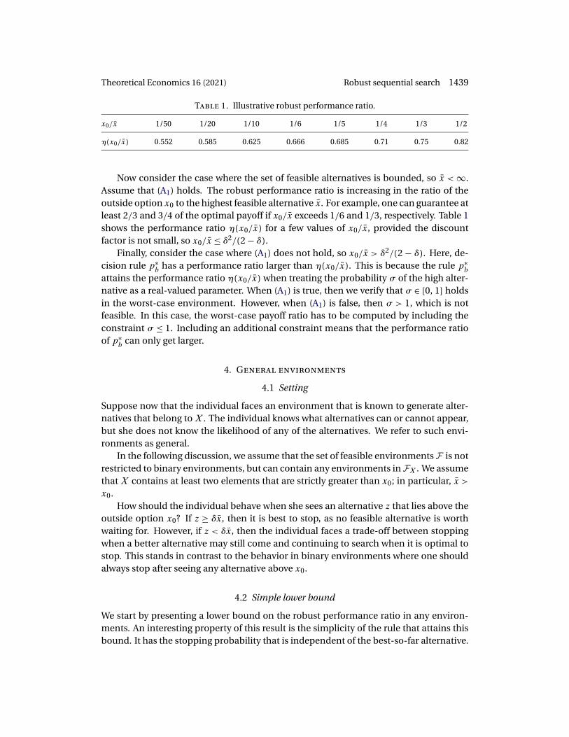
Table 1. Illustrative robust performance ratio.

x0/x̄ 1/50 1/20 1/10 1/6 1/5 1/4 1/3 1/2

η(x0/x̄) 0.552 0.585 0.625 0.666 0.685 0.71 0.75 0.82

Now consider the case where the set of feasible alternatives is bounded, so x̄ <∞.Assume that (A1) holds. The robust performance ratio is increasing in the ratio of theoutside option x0 to the highest feasible alternative x̄. For example, one can guarantee atleast 2/3 and 3/4 of the optimal payoff if x0/x̄ exceeds 1/6 and 1/3, respectively. Table 1shows the performance ratio η(x0/x̄) for a few values of x0/x̄, provided the discountfactor is not small, so x0/x̄≤ δ2/(2 − δ).

Finally, consider the case where (A1) does not hold, so x0/x̄ > δ2/(2 − δ). Here, de-

cision rule p∗b has a performance ratio larger than η(x0/x̄). This is because the rule p∗

b

attains the performance ratio η(x0/x̄) when treating the probability σ of the high alter-native as a real-valued parameter. When (A1) is true, then we verify that σ ∈ [0, 1] holdsin the worst-case environment. However, when (A1) is false, then σ > 1, which is notfeasible. In this case, the worst-case payoff ratio has to be computed by including theconstraint σ ≤ 1. Including an additional constraint means that the performance ratioof p∗

b can only get larger.

4. General environments

4.1 Setting

Suppose now that the individual faces an environment that is known to generate alter-natives that belong to X . The individual knows what alternatives can or cannot appear,but she does not know the likelihood of any of the alternatives. We refer to such envi-ronments as general.

In the following discussion, we assume that the set of feasible environments F is notrestricted to binary environments, but can contain any environments in FX . We assumethat X contains at least two elements that are strictly greater than x0; in particular, x̄ >x0.

How should the individual behave when she sees an alternative z that lies above theoutside option x0? If z ≥ δx̄, then it is best to stop, as no feasible alternative is worthwaiting for. However, if z < δx̄, then the individual faces a trade-off between stoppingwhen a better alternative may still come and continuing to search when it is optimal tostop. This stands in contrast to the behavior in binary environments where one shouldalways stop after seeing any alternative above x0.

4.2 Simple lower bound

We start by presenting a lower bound on the robust performance ratio in any environ-ments. An interesting property of this result is the simplicity of the rule that attains thisbound. It has the stopping probability that is independent of the best-so-far alternative.


Theorem 2. Let F ⊂ FX . The robust performance ratio satisfies

R∗(F ) ≥ 14

.

The lower bound 1/4 is attained by the decision rule pg given by

pg(y ) = 1 − δ2 − δ for all y ≥ x0.

Remark 1. The lower bound 1/4 on the robust performance ratio is tight. The robustperformance ratio is equal to 1/4 (thus, rule pg is robust) when the setX is unbounded,so x̄= ∞.

The robust performance ratio is clearly the lowest when x̄ is the highest. We sketchthe argument regarding why the robust performance ratio of 1/4 is attained when x̄= ∞.In this setting, regardless of how large the best-so-far alternative already is, an infinitelylarger alternative can still appear. Hence, the value of the best-so-far alternative plays norole when designing a robust decision rule. We can thus limit attention to rules that havea constant probability of stopping q for some q ∈ [0, 1]. The worst-case environmentgenerates a high alternative z that occurs with extremely small probability σ , but that issufficiently large so that it is worth waiting for. A greater qmeans a greater probability ofstopping before z realizes, but also a shorter delay before stopping and obtaining z afterit has realized. The performance ratio is attained as z → ∞ and σ → 0 such that theoptimal payoff of waiting for the first realization of z goes to infinity. Because y/z→ 0,the individual essentially cares only about getting z. The performance ratio takes theform

q

1 − δ(1 − q)

(1 − q

1 − δ(1 − q)

). (6)

To understand (6), it is useful to think of 1 − δ as the exogenous probability that thesearch stops in the current round and yields zero payoff. Then the expression

q

1 − δ(1 − q)= q+ δ(1 − q)q+ δ2(1 − q)2q+ · · ·

can be seen as the expected probability of getting z after it has been realized. To interpretthe second factor in (6), consider the following expressions. First,

δσ(1 + δ(1 − σ ) + δ2(1 − σ )2 + · · · ) = δσ

1 − δ(1 − σ )

is the expected probability of not stopping before z realizes under the optimal rule,where the probability of stopping in each round is 1 − δ. Second,

(1 − q)δσ(1 + (1 − q)δ(1 − σ ) + (1 − q)2δ2(1 − σ )2 + · · · ) = (1 − q)δσ

1 − (1 − q)δ(1 − σ )


is the expected probability of not stopping before z realizes under the rule q, where theprobability of stopping in each round is (1 − δ)q. As σ tends to 0, the ratio of the latterto the former is

(1 − q)δσ1 − (1 − q)δ(1 − σ )

· 1 − δ(1 − σ )δσ

σ→0−−−→ (1 − q)(1 − δ)1 − δ(1 − q)

= 1 − q

1 − δ(1 − q).

We can now interpret (6). The first factor in (6) is the expected probability of obtaining zafter it has realized. The second factor in (6) is the expected probability of not stoppingbefore z realizes for the first time. Setting q/(1−δ(1−q)) equal to 1/2, so q= (1−δ)(2−δ), maximizes (6), leading to the performance ratio 1/4.

4.3 Bounded environments

In the following discussion, we present the robust performance ratio for the case wherethe outside option x0 is not too small in general environments in which alternatives arebounded, so x̄ <∞. We call these environments bounded. Recall the definition of ηgiven by (5) in Section 3 and define

f (x, t ) =

⎧⎪⎨⎪⎩

(1 − δ)(1 − t )(1 − δ)(1 − t ) + (

√t − √

x)2if x < t,

1 if x≥ t.

Theorem 3. Let x̄ <∞ and let (A1) hold. There exists a constant λ ∈ (1/90, 7/100) suchthat if

x0

x̄≥ λ,

then the robust performance ratio is

R∗(FX ) = η(x0

x̄

).

It is attained by the robust decision rule p∗g given by

p∗g(y ) = f

(y

x̄, η

(x0

x̄

))for y ∈ [x0, x̄].

Theorem 3 shows that if the outside option is not too small relative to the highestpossible alternative, in the sense that x0/x̄ ≥ λ, then the robust performance ratio ingeneral environments is the same as it is in binary environments. Remarkably, the con-stant λ is very small. We prove that λ < 7/100. Moreover, we numerically (up to precision10−8) find that

λ≈ 0.01120000,

where 1/90 < 0.0112 < 1/89 (see Remark 3 in Appendix A.5). Thus, as x0/x̄ increasesfrom 0 to a mere 1/89, the robust performance ratio climbs from at least 1/4 (by Theo-rem 2) to at least 1/2 (by Theorem 3). In particular, one can guarantee at least 2/3 and


Figure 1. The black line shows the robust performance ratio in binary and general environ-ments with x0/x̄ ≥ λ (see Theorem 3). The grey line shows the robust performance ratio in bi-nary environments with x0/x̄ < λ (see Theorem 1). The dotted line shows the hypothetical robustperformance ratio in general environments with x0/x̄ < λ (as conjectured from Theorem 2 andRemark 1).

3/4 of the optimum if the outside option exceeds 1/6 and 1/3 of the highest feasiblealternative, respectively. Figure 1 illustrates the robust performance ratio in differentsettings.

Notice that the rule p∗b that attains the robust performance ratio in binary environ-

ments no longer has this property in general environments. This is because it stopsimmediately when an alternative above the outside option arrives. In contrast, the ro-bust rule p∗

g randomizes whenever it is worth waiting for a higher alternative. Of course,as binary environments belong to the set of general environments, p∗

g is also robust inbinary environments as long as x0/x̄≥ λ.

Why is the robust performance ratio in general environments the same as it is inbinary environments when x0/x̄≥ λ? When using rule p∗

g, the worst-case general envi-ronments are binary environments that randomize between 0 and x̄. These are the sameworst-case environments we found in the binary environment setting. We verify that theperformance ratio of p∗

g is equal to η(x0/x̄), which is the robust performance ratio in bi-nary environments. This means that p∗

g is robust in general environments because theperformance ratio can only become worse if one adds more environments. However,when x0/x̄ < λ, then the performance ratio of p∗

g is strictly smaller in general environ-ments than it is in binary environments. This is because the worst-case environmentnow randomizes between 0 and an alternative strictly below x̄.

On a final note, we comment on re-optimization. When the individual draws analternative z that lies above the outside option x0, then the future looks like the originalproblem except it is as if now the outside option is larger, namely, equal to z. One mightbe tempted to switch to a decision rule that is designed for this outside option. However,such re-optimization is not allowed in our model. This is investigated in a follow-uppaper by Schlag and Sobolev (2020).


5. Nonstationary decision rules

5.1 Setting

So far we have restricted attention to stationary decision rules. The behavior prescribedby these rules does not depend on time or history. It depends only on the highest alter-native drawn so far. We now demonstrate that our results remain unchanged if we allowfor nonstationary decision rules.

We update our definitions introduced in Section 2 to incorporate the dependence ofdecision rules on histories.

Let ht = (x0, x1, � � � , xt ) be a history of alternatives up to round t for t = 0, 1, 2, � � � .A decision rule p prescribes for each history ht a probability p(ht ) of stopping after thathistory. A decision rule p is stationary if p(x0, x1, � � � , xt ) = p(x0, x′

1, � � � , x′t ′ ) whenever

max{x0, x1, � � � , xt } = max{x0, x′1, � � � , x′

t ′ }. Let P be the set of all decision rules and let Pstbe the set of stationary decision rules.

We say that a history ht is consistent with an environment F if it has a strictly positiveprobability under F . Let F ⊂ FX be a set of feasible environments. For an environmentF ∈ F , letH(F ) be the set of all finite histories consistent with F .

Consider an environment F ∈ F and a history ht ∈H(F ). With abuse of notation letht+1 = (ht , xt+1 ). LetUp(F , ht ) be the expected payoff of a decision rulep under F whenthe history is ht , so

Up(F , ht ) = p(ht ) max{x0, x1, � � � , xt } + (1 −p(ht )

)δ

∫XUp

(F , (ht , xt+1 )

)dF(xt+1 ).

Let V (F , ht ) be the optimal payoff under F when the history is ht , so

V (F , ht ) = supp∈P

Up(F , ht ).

Note that V (F , ht ) ≥ max{x0, x1, � � � , xt } ≥ x0 > 0.The performance ratioRp(F ) of a decision rulep is defined as the lowest payoff ratio

over all feasible environments and all histories that are consistent with each of thoseenvironments:

Rp(F ) = infF∈F

infht∈H(F )

Up(F , ht )V (F , ht )

.

So the performance ratio is the largest fraction of the optimal payoff that a decisionrule guarantees no matter what environment in F the individual faces, in each roundof search and after each history of alternatives that can be generated with a positiveprobability. As in Section 2, the highest possible performance ratio is called robust, andis given by

R∗(F ) = supp∈P

Rp(F ).

A decision rule p∗ is called robust if it attains the robust performance ratio, so Rp∗(F ) =R∗(F ).


5.2 Randomization

Before describing the results, let us show that randomization is essential for robustsearch. In other words, deterministic rules are not robust, provided there is an alter-native worth waiting for. This insight appeared informally in Section 2.3. Here we proveit formally.

A decision rule p is called deterministic if for each history, the individual either stopssearching or continues to search with certainty. Formally, this means that p(ht ) ∈ {0, 1}for every possible history ht . Let p1 be the deterministic rule that stops searching aftereach history, so p1(ht ) = 1 for all ht .

Let F ⊂ FX be the set of feasible environments. Let F0 and Fx̄ be the environmentsthat generate alternative 0 and alternative x̄ with certainty, respectively. We show thatdeterministic decision rules are not robust when these two environments are feasibleand x̄ is worth waiting for, in the sense that δx̄ > x0.

Proposition 1. Let F0, Fx̄ ∈ F and let δx̄ > x0. Then

Rp(F ) ≤Rp1 (F ) = x0

δx̄< R∗(F ).

We explain the above result. The rule p1 that does not search has a performance ra-tio equal to x0/(δx̄). This is because the worst-case environment for this rule is Fx̄. Thisratio can be arbitrarily small if the outside option x0 is close to 0 or if the highest alter-native x̄ is very large. The first inequality in Proposition 1 shows that no deterministicrule can outperform the rule p1 that does not search. The second inequality shows thatdeterministic rules are not robust.

Remark 2. Proposition 1 sheds light on the performance of Bayesian rules. These arethe rules used by Bayesian decision makers who maximize their expected payoffs forsome prior. Any such rule prescribes to stop the search if the best-so-far alternative isbetter than the expected continuation payoff under the given prior and to continue thesearch otherwise. Indifference between stopping and continuing under a given prior isnongeneric in the sense that it does not hold under an open set of priors in the neigh-borhood of that prior. Hence, Bayesian rules are generically deterministic. So by Propo-sition 1, Bayesian rules are generically not robust.

5.3 Binary environments

Here we show that that there is no loss of generality to restrict attention to stationaryrules when investigating robust performance in binary environments. In other words,any rule can be outperformed by an appropriately chosen stationary rule.

Proposition 2. For each p ∈ P there exists p̃ ∈ Pst such that Rp(BX ) ≤Rp̃(BX ).

By Proposition 2, it is immediate that Theorem 1 extends to nonstationary decisionrules.

Corollary 1. Theorem 1 holds when the set of decision rules is P .


5.4 General environments

Let us now consider the performance of nonstationary rules in general environments asdefined in Section 4.

Theorem 2 clearly continues to hold as it identifies a lower bound that remains validif the set of decision rules becomes richer.


We apply Corollary 1 to prove the next result.


Proof. By Corollary 1, the robust performance ratio in binary environments isη(x0/x̄).So the robust performance ratio in general environments can only be smaller thanη(x0/x̄). However, by Theorem 3, the stationary decision rule p∗

g attains η(x0/x̄) ingeneral environments. Hence, the rule p∗

g is robust in general environments, with orwithout the restriction to stationary rules.

Finally, we hasten to point out that we do not extend Remark 1 to nonstationaryrules in this paper. Whether the performance ratio of 1/4 is robust when the set X ofalternatives is unbounded remains an open question.

6. Conclusion

It is difficult to search under the classic objectives of expected utility maximization whenthe distribution of alternatives is not known. In fact, the literature has not producedsatisfactory insights into how to search in this setting. In this paper, we identify thatthis difficulty is due to the desire to achieve the very highest payoff for the given beliefs.Namely, we find that it is easier to search if one reduces the target and replaces “veryhighest” by “relatively high.” The ease refers to the ability to derive a solution for a verygeneral setting, the simplicity of our algorithm, and the minimality of assumptions oneneeds to impose on the environment.

Many interesting topics remain that have not been addressed in this paper. Are theregood rules that allow the individual to reoptimize after each new alternative arrives?How do we search if costs are additive? What is the robust performance ratio when thereis no free recall? What if alternatives do not arrive according to an i.i.d. process?

The methodology developed in this paper is applicable to a spectrum of dynamicdecision making problems and should spark future research.

Appendix: Proofs

A.1 Auxiliary definitions and results

Let rp(y ) be given by

rp(y ) = infF∈BX

Up(F , y )V (F , y )

= infz∈X ,z>x0,σ∈[0,1]

Up(F(z,σ ), y )V (F(z,σ ), y )

for y ≥ x0. (7)


So rp(y ) is the smallest payoff ratio of a stationary rule p under binary environmentswhen the best-so-far alternative is y. Observe that in the model with binary environ-ments, the performance ratio of a decision rule p is given by

Rp(BX ) = rp(x0 ). (8)

This is because whenever a best-so-far alternative is y > x0, the individual knows thatno better alternative will ever arrive and, thus, stops immediately. The payoff ratio is 1in this case. So the performance ratio Rp(BX ) is determined by the smallest payoff ratiowhen the best-so-far alternative is x0.

The ratio rp(x0 ) is our main instrument for finding the performance ratio of p notonly in binary environments BX , but also in general environments FX .

We now find rp(y ) for a given decision rulep. To simplify the exposition of the proofs,we introduce some notation. For x0 ≤ y < z and s ∈ [0, 1), let κp andmp be given by

κp(y ) = p(y )1 − δ+ δp(y )

(9)

and

mp(y, z, s) = (1 − s)κp(y )y + (1 − κp(y )

)κp(z)sz

1 − sκp(y ). (10)

Note that 1 − sκp(y )> 0, because κp(y ) ∈ [0, 1] and s < 1. For σ ∈ [0, 1], let

sσ = δσ

1 − δ+ δσ . (11)

The next lemma shows that κp(y )y and mp(y, z, sσ ) are the payoffs of rule p when theenvironment is F(z,σ ) for the cases of z ≤ y and z > y, respectively.

Lemma 1. We have

Up(F(z,σ ), y ) ={κp(y )y if z ≤ y,

mp(y, z, sσ ) if z > y.(12)

Proof. Let z ≤ y. By (1), the payoff of decision rule p in a binary environment F(z,σ )

is given by Up(F(z,σ ), y ) = p(y )y + (1 − p(y ))δUp(F(z,σ ), y ). Solving this equation forUp(F(z,σ ), y ) and using (9) yields

Up(F(z,σ ), y ) = p(y )y1 − δ+ δp(y )

= κp(y )y if z ≤ y. (13)

Next, let z > y. By (1),

Up(F(z,σ ), y ) = p(y )y + (1 −p(y )

)δ(σUp(F(z,σ ), z) + (1 − σ )Up(F(z,σ ), y )

). (14)


Inserting y = z into (13) yieldsUp(F(z,σ ), z) = κp(z)z. Inserting this into (14) and solvingfor Up(F(z,σ ), y ) yields

Up(F(z,σ ), y ) = p(y )y + (1 −p(y )

)δσκp(z)z

1 − δ(1 − σ )(1 −p(y )

) .

Finally, we use (9) to replacep(y ) by (1−δ)κp(y )/(1−δκp(y )) and we use (11) to replaceσ by (1−δ)sσ

δ(1−sσ ) . Note that sσ ≤ δ < 1, so δ(1 − sσ )> 0 and κp(y ) ≥ 0, so 1 −δκp(y )> 0. Aftersimplification, we obtain

Up(F(z,σ ), y ) = (1 − sσ )κp(y )y + (1 − κp(y )

)κp(z)sσz

1 − sσκp(y )=mp(y, z, sσ ) if z > y.

We now characterize rp(y ). Below we repeatedly use the infimum operator. When-ever the infimum is taken over an empty set, we follow the convention that inf(∅) = +∞.

Proposition 3. Let y ∈X ∪ {x0} and z ∈X such that x0 ≤ y < z. For each rule p,

rp(y ) ≤ infs∈( yz ,δ]

mp(y, z, s)sz

. (15)

Moreover, if p(y ) is weakly increasing in y, then

rp(y ) = min{κp(y ), inf

z∈X ,z>x0,s∈( yz ,δ]

mp(y, z, s)sz

}. (16)

Proof. Let p be a decision rule, let y ∈ [x0, x̄], and let F(z,σ ) ∈ BX . First, we findV (F(z,σ ), y ). Solving (2) for cF(z,σ ) and using (11), we obtain

cF(z,σ ) = δσz

1 − δ+ δσ = sσz.

By (3),

V (F(z,σ ), y ) = max{y, cF(z,σ ) } = max{y, sσz}. (17)

Next,

rp(y ) = infz∈X ,z>x0,σ∈[0,1]

Up(F(z,σ ), y )V (F(z,σ ), y )

= min{

infz∈X ,σ∈[0,1]s.t. x0<z≤y

Up(F(z,σ ), y )V (F(z,σ ), y )

, infz∈X ,σ∈[0,1]

s.t. cF(z,σ )≤y<z

Up(F(z,σ ), y )V (F(z,σ ), y )

,

infz∈X ,σ∈[0,1]

s.t. y<cF(z,σ )<z

Up(F(z,σ ), y )V (F(z,σ ), y )

}

= min{

infz∈X ,s∈[0,δ]s.t. x0<z≤y

κp(y )y

y, infz∈X ,s∈[0,δ]s.t. sz≤y<z

mp(y, z, s)y

,


infz∈X ,s∈[0,δ]

s.t. y<sz

mp(y, z, s)sz

}. (18)

The first equality is by (7), the second equality is by partitioning the set {(z, σ ) : z ∈X , z > x0, σ ∈ [0, 1]} into three subsets, and the third equality is by (17), Lemma 1, andthe property that for each s ∈ [0, δ], there is a unique σ ∈ [0, 1] such that s = sσ . Theinequality (15) follows from (18).

To prove (16), consider sz ≤ y < z. By (10), we have

mp(y, z, s) ≥ (1 − s)κp(y )y + (1 − κp(y )

)κp(y )sy

1 − sκp(y )= κp(y )y,

where the inequality is because p(z) is increasing by assumption and, hence, κp(z)z ≥κp(y )y, and the equality is by the simplification of the expression. Moreover, by (10), wehavemp(y, z, 0) = κp(y )y. Therefore,

infz∈X ,s∈[0,δ]s.t. sz≤y<z

mp(y, z, s)y

= κp(y )y

y= κp(y ). (19)

So (16) follows from (18) and (19).

We now aim to compute rp(x0 ) using Proposition 3. It is apparent from Proposition 3that the difficulty in finding rp(x0 ) is the minimization of mp(x0, z, s)/(sz) with respectto (z, s). For our proofs, we minimizemp(x0, z, s)/(sz) with respect to s for s ∈ (0, 1). Wethen show that the solution is feasible, so it attains rp(y ), provided (A1) holds.

Lemma 2. Let z ∈X with z > x0. Suppose that x0 ≤ y < z ≤ x̄. Then

infs∈(0,1]

mp(y, z, s)sz

=⎧⎨⎩

1z

(κp(y )

√y +

√(1 − κp(y )

)(κp(z)z− κp(y )y

))2if y < κp(z)z,

κp(z) if y ≥ κp(z)z.

Moreover, the value of s that minimizesmp(y, z, s)/(sz) is given by

s∗(y, z) =

⎧⎪⎨⎪⎩

(κp(y ) +

√(1 − κp(y )

)(κp(z)z

y− κp(y )

))−1

if y < κp(z)z,

1 if y ≥ κp(z)z.

(20)

Proof. Assume x0 ≤ y < z ≤ x̄. Let us find a solution s∗(y, z) to the problem

infs∈(0,1]

mp(y, z, s)sz

= infs∈(0,1]

(1 − s)κp(y )y + (1 − κp(y )

)κp(z)sz(

1 − sκp(y ))sz

.

We have

∂

∂s

(mp(y, z, s)

sz

)= κp(y )(

1 − sκp(y ))2s2z

G(s), (21)


where

G(s) = (κp(z)z

(1 − κp(y )

) − κp(y )y)s2 + 2κp(y )ys− y.

The expression κp(y )/((1 − sκp(y ))2s2z) is positive when s ∈ (0, 1] and z > y ≥ x0 > 0.So the sign of (21) is determined by G(s). Observe that G(s) is increasing for s ∈ (0, 1],because

dG(s)ds

= 2κp(z)z(1 − κp(y )

)s+ 2κp(y )y(1 − s) ≥ 0.

Also observe thatG(0) = −y andG(1) = (1 − κp(y ))(κp(z)z− y ).Suppose that κp(z)z − y ≤ 0, so G(1) ≤ 0. It follows that G(s) ≤ 0 for all s ∈ [0, 1].

Thus, s∗(y, z) = 1 is a solution.Alternatively, suppose that κp(z)z − y > 0, so G(1) ≥ 0. Then there exists a solution

ofG(s) = 0 on (0, 1]. The quadratic equationG(s) = 0 has two solutions,

s1 = 1

kp(y ) + √D

and s2 = 1

kp(y ) − √D

,

where

D= (1 − κp(y )

)(κp(z)z

y− κp(y )

).

Because 1 ≥ κp(z)z > y, we have√D > 1 − κp(y ) > 0, so s1 ∈ (0, 1) and s2 /∈ [0, 1]. It

follows that s∗(y, z) = s1 is a solution.Thus, we have shown (20). It remains to substitute s = s∗(y, z) into mp(y, z, s)/(sz).

For the case of κp(z)z− y ≤ 0, we obtain

infs∈(0,1]

mp(y, z, s)sz

= mp(y, z, 1)z

= κp(z).

For the case of κp(z)z− y > 0, we obtain, after simplification,

infs∈(0,1]

mp(y, z, s)sz

= mp(y, z, s1 )z

= 1z

(κp(y )

√y +

√(1 − κp(y )

)(κp(z)z− κp(y )y

))2.

A.2 Proof of Theorem 1

Let q ∈ [0, 1], and let pq be a decision rule given by pq(x0 ) = q and pq(y ) = 1 for ally > x0. To prove Theorem 1, we use the notation and results from Appendix A.1. Weshow that under assumption (A1), the rule pq∗ with

q∗ = 1 − δ

2 − δ+ 12

(x0

x̄−

√x0

x̄

(x0

x̄+ 8

)) (22)

maximizes Rpq (BX ) among all q ∈ [0, 1]. So this rule is robust. We then verify thatRpq∗ (BX ) = η(x0/x̄).


Recall the notation rp, κp, andmp for a rule p introduced in Appendix A.1 by (7), (9),and (10), respectively. By (8) and Proposition 3,

Rpq (BX ) = rpq (x0 ) = min{κpq (x0 ), inf

z∈X ,z>x0,s∈(x0z ,δ]

mpq (x0, z, s)

sz

}.

Let z ∈X with z > x0 and let s ∈ (0, 1]. Note that κpq(z) = 1. Let

k= κpq (x0 ) = q

1 − δ+ δq . (23)

By (10), we have

mpq (x0, z, s) = (1 − s)κpq (x0 )x0 + (1 − κpq (x0 )

)κpq (z)sz

1 − sκpq (x0 )= (1 − s)kx0 + (1 − k)sz

1 − sk .

Observe thatmpq (x0, z, s)/(sz) is decreasing in z, because

ddz

(mpq (x0, z, s)

sz

)= d

dz

((1 − s)kx0 + (1 − k)sz

(1 − sk)sz

)= − (1 − s)kx0

(1 − sk)sz2 ≤ 0,

sompq (x0, z, s)/(sz) attains its infimum as z→ x̄. We thus obtain

Rpq (BX ) = min{k, inf

s∈(x0x̄ ,δ]

(1 − s)kx0

x̄+ (1 − k)s

(1 − sk)s

}.

Note that each k ∈ [0, 1] corresponds to a unique q ∈ [0, 1], so

R∗(BX ) = supq∈[0,1]

Rpq (BX ) = supk∈[0,1]

min{k, inf

s∈(x0x̄ ,δ]

(1 − s)kx0

x̄+ (1 − k)s

(1 − sk)s

}. (24)

Consider the case of x̄= ∞, so x0/x̄= 0. By (24), we obtain

R∗(BX ) = supk∈[0,1]

min{k, inf

s∈(0,δ]

(1 − k)s

(1 − sk)s

}= supk∈[0,1]

min{k, 1 − k} = 12

.

The maximum is attained at k∗ = 1/2. By (23), k∗ = 1/2 corresponds to q∗ = (1 −δ)/(2 −δ). We have thus shown (22) for the case of x0/x̄= 0.

Next, to address the case of x̄ <∞, we first find

ρ∗(x0, x̄) = supk∈[0,1]

min{k, infs∈(0,1]

mpq (x0, x̄, s)

sx̄

}.

We later show that R∗(BX ) = ρ∗(x0, x̄). By Lemma 2 with y = x0 and z = x̄, we have

infs∈(0,1]

mpq (x0, x̄, s)

sx̄= (k√x+

√(1 − k)(1 − kx)

)2,


where we denote

x= x0

x̄.

Thus, we obtain

ρ∗(x0, x̄) = supk∈[0,1]

min{k,

(k√x+

√(1 − k)(1 − kx)

)2}. (25)

Observe that

ddk

(k√x+

√(1 − k)(1 − kx)

) = −(√

(1 − k)x−√

1 − kx)2

2√

(1 − k)(1 − kx)≤ 0. (26)

So the term (k√x + √

(1 − k)(1 − kx))2 is decreasing in k. We thus conclude that thesolution of (25) is the solution to the equation

k= (k√x+

√(1 − k)(1 − kx)

)2. (27)

Because the left-hand side of (27) is strictly increasing and the right-hand side of (27) isdecreasing in k for k ∈ [0, 1], the solution of (27) is unique. By substituting

k∗ = 12

+ 18

(x+

√x(x+ 8)

)(28)

into (27), we verify that k∗ is the solution of (27). By (23), k∗ corresponds to q∗ as givenby (22). Finally, by (5) and (25),

ρ∗(x0, x̄) = k∗ = η(x).

It remains to show that thatR∗(BX ) = ρ∗(x0, x̄). Observe that by (24), we haveR∗(BX ) =ρ∗(x0, x̄) if s∗(k∗ ) is feasible in (24); specifically, if s∗(k∗ ) ∈ (x0/x̄, δ]. By Lemma 2, fork ∈ [0, 1],

s∗(k) =(k+

√(1 − k)

(x̄

x0− k

))−1

=√x

k√x+

√(1 − k)(1 − kx)

. (29)

To verify that s∗(k∗ )> x0/x̄= x, observe that s∗(k) is increasing in k, so

s∗(k∗) ≥ s∗(0) = √

x > x.

Finally, we verify that s∗(k∗ ) ≤ δ, provided (A1) holds, so x≤ δ2/(2 − δ). It is easy to seefrom (29) that s∗(k) is increasing in both k and x. Moreover, by (28), k∗ is increasing in x.Consequently, s∗(k∗ ) is increasing in x. So to verify that s∗(k∗ ) ≤ δ for all x≤ δ2/(2 − δ),it suffices to verify it for x= δ2/(2 − δ). Substituting x= δ2/(2 − δ) into (28) yields k∗ =1/(2 − δ). Next, substituting both x = δ2/(2 − δ) and k∗ = 1/(2 − δ) into (29) yieldss∗(k∗ ) = δ. We, thus, have verified that s∗(k∗ ) is in (x0/x̄, δ] whenever (A1) holds.


A.3 Connecting general and binary environments

As a preliminary step before proving Theorems 2 and 3, we show that the performanceratio of a regular decision rule p is equal to rp(x0 ), where rp is defined in Appendix A.1.

Definition 1. Rule p is regular if it satisfies two conditions:

(i) p(y ) is weakly increasing in y

(ii) rp(y ) is weakly increasing in y.

Regularity is an intuitive condition. Condition (i) means that the individual is morelikely to accept a greater best-so-far alternative. Condition (ii) is a “free-disposal” prop-erty. If this property does not hold, so a better best-so-far alternative leads to a lowerguaranteed payoff ratio, then the individual could be better off by destroying some partof the value of the best-so-far alternative.

The next proposition shows that when determining the performance ratio of anyregular decision rule in general environments, we can restrict attention to binary envi-ronments and to a single best-so-far alternative y = x0. This is a dramatic simplificationof the problem, because binary environments are easy to deal with and we do not needto worry about a multitude of possible values of best-so-far alternatives.

Proposition 4. Suppose that p is regular. Then Rp(FX ) = rp(x0 ).

We hasten to point out that by Proposition 4, the restriction to binary environmentsis without loss of generality only when dealing with regular rules. The rule p∗

b identifiedin Theorem 1 is not regular, so Proposition 4 does not apply to this rule. In fact, it is easyto verify that p∗

b is not robust in general environments.

Proof of Proposition 4. The proof relies on two lemmas. We first present the state-ments of these two lemmas and show how they prove Proposition 4. Then we prove thetwo lemmas.

Let Y0 be the set of all possible best-so-far alternatives:

Y0 =⋃F∈FX

Y (F ) = {y ∈X ∪ {x0} : y ≥ x0

}.

Lemma 3 shows that the smallest payoff ratio does not change if we expand the set Y (F )for each F ∈ FX to Y0.

Lemma 3. We have infF∈FX ,y∈Y (F )Up(F ,y )V (F ,y ) = infF∈FX ,y∈Y0

Up(F ,y )V (F ,y ) .

The proof is deferred to the end of this subsection.Lemma 4 proves that when determining the worst-case payoff ratio of a regular de-

cision rule in general environments, we can restrict attention to binary environments.


Lemma 4. Suppose that p is regular. Then, for each y ∈ Y0,

infF∈FX

Up(F , y )V (F , y )

= rp(y ). (30)

The proof is deferred to the end of this subsection.From Lemmas 3 and 4, we obtain

Rp(FX ) = infF∈FX

(inf

y∈Y (F )

Up(F , y )V (F , y )

)= infy∈Y0

(infF∈FX

Up(F , y )V (F , y )

)= infy∈Y0

rp(y ) = rp(x0 ),

where the first equality is by the definition of Rp(FX ), the second equality is byLemma 3, the third equality is by Lemma 4, and the fourth equality is because rp is reg-ular. This completes the proof of Proposition 4.

We now prove Lemmas 3 and 4.

Proof of Lemma 3. For each y ∈ Y0, let F̂X(y ) be the set of all environments in whichy is a feasible best-so-far alternative:

F̂X(y ) = {F ∈ FX : y ∈ Y (F )

}.

Using this notation, we can equivalently express Rp(FX ) as

Rp(FX ) = infy∈Y0

(inf

F∈F̂X (y )

Up(F , y )V (F , y )

)= infy∈Y0

(inf

F∈Closure(F̂X (y ))

Up(F , y )V (F , y )

). (31)

It remains to show that Closure(F̂X(y )) = FX for each y ∈ Y0. Intuitively, if there is adistribution F /∈ F̂X(y ), so y is not in the support of F , then there is another distributionthat is arbitrarily close to F and yet places a positive, albeit arbitrarily small, probabilityon y.

Since x0 ∈ Y (F ) for all F ∈ FX , we have F̂X(x0 ) = FX . Now consider y ∈ Y0\{x0}. LetF ∈ FX . Let Dy be the Dirac distribution that assigns probability 1 on y. Let (Fk )∞k=1 bea sequence of distributions given by

Fk = 1kDy +

(1 − 1

k

)F , k ∈N,

so limk→∞ Fk = F . Notice that Fk ∈ FX for all k ∈ N. By construction, we have {y} ⊂Y (Dy ) ⊂ Y (Fk ) and, thus, Fk ∈ F̂X(y ) for all k ∈ N, so F ∈ Closure(F̂X(y )). Since theabove statement is true for all F ∈ FX , it follows that Closure(F̂X(y )) = FX . The state-ment of the lemma is then immediate by (31).

Proof of Lemma 4. Let p be a regular rule. Fix any best-so-far alternative y ∈ Y0 andany environment F ∈ FX . We show that there exist a probability σ ∈ [0, 1] and alterna-tives w, z ∈ Y (F ) with y ≤w≤ z ≤ x̄ such that

Up(F , y )V (F , y )

≥ Up(F , w)V (F , w)

≥ Up(F(z,σ ), w)V (F(z,σ ), w)

. (32)


Then, by (32), the definition of rp, and the regularity of rule p, we obtain

Up(F , y )V (F , y )

≥ Up(F(z,σ ), w)V (F(z,σ ), w)

≥ rp(w) ≥ rp(y ).

This implies (30), because BX ⊂ FX and F is an arbitrary environment in FX . To com-plete the proof, it remains to show (32).

Let w be an alternative that satisfies

Up(F , w) = minx∈Y (F ),x≥y

Up(F , x). (33)

By assumption, F has a finite support, so Y (F ) is finite. Therefore, w is well defined.Because Up(F , w) ≤ Up(F , y ) by (33), and V (F , w) ≥ V (F , y ) by (3) and the constraintw≥ y, we obtain the first inequality in (32).

Let us show the second inequality in (32). Recall that by (1),

Up(F , w) = p(w)w+ (1 −p(w)

)δ

∫ x̄

0Up

(F , max{w, x}

)dF(x). (34)

Let cF be the reservation value of F as given by (2). Subsequently, we omit the subscript,so c = cF . As δ < 1, it is easy the verify that

0 ≤ c/δ < x̄. (35)

Suppose that w ≥ c. Then, by (3), V (F , w) =w. Moreover, V (F(w,1), w) =w. Also, by(33) and (34),

Up(F , w) ≥ p(w)w+ (1 −p(w)

)δUp(F , w).

Solving this inequality yields

Up(F , w) ≥ p(w)w1 − δ(1 −p(w)

= κp(w)w=Up(F(w,1), w),

where the first equality is by (9) and the second equality is by Lemma 1 (see Ap-pendix A.1). Thus, we have obtained the second inequality in (32) with F(z,σ ) = F(w,1).

Next suppose that w < c. To show the second inequality in (32), we first bound theexpression

∫ x̄0 Up(F , max{w, x}) dF(x) from below. For each x ∈ Y (F ), let

u(x) ={Up(F , w), x≤ c,

Up(F , x), x > c.(36)

Since w< c, by (33) and (36), we have

Up(F , max{w, x}

) ≥ u(x) for all x ∈ [0, x̄]. (37)


Figure 2. Two cases that arise when solving (38) and (39). The dotted lines show the values ofu(x) for x in the discrete support of F . The solid lines show uconv(x).

Let us find alternatives w′ and z in Y (F ) with w ≤ w′ ≤ c/δ ≤ z ≤ x̄ and a probabilityσ ∈ [0, 1] such that ∫ x̄

0u(x) dF(x) ≥ (1 − σ )u

(w′) + σu(z), (38)

(1 − σ )w′ + σz = c

δ. (39)

We apply the convexification method as in Kamenica and Gentzkow (2011). Con-sider the greatest convex function uconv : [0, x̄] → R such that uconv(x) ≤ u(x) for allx ∈ Y (F ), as shown in Figure 2. This is known as the convex closure of u. Clearly, tosatisfy (38) and (39), the alternatives w′ and z must be the closest values in Y (F ) to theleft and to the right of c/δ, respectively, such that u(w′ ) = uconv(w′ ) and u(z) = uconv(z).Then σ is derived from (39). In particular, if u(c/δ) = uconv(c/δ), then w′ = z = c/δ andσ is arbitrary.

Let (w′, z, σ ) satisfy (38) and -(39). Observe that the straight line through points(w′, u(w′ )) and (z, u(z)) is weakly below the graph of u. Moreover, this straight line hasa nonnegative slope, because by (33), we have u(w) ≤ u(x) for all x ≥ w. So we canconclude that

u(w′) ≤ u(x) for all x≥w′,

u(z) ≤ u(x) for all x≥ z.(40)

We consider two cases illustrated by Figure 2(a) and (b), withw′ > c andw′ = c. It is clearthat w′ < c cannot occur, because u(x) is constant for x≤ c (see Figure 2).

Case 1. Suppose that w′ > c. We have

u(z) = p(z)z+ (1 −p(z)

)δ

∫ x̄

0u(max{z, x}

)dF(x) ≥ p(z)z+ (

1 −p(z))δu(z),


where the equality is by (34) and (36), and the inequality is by (40). Solving the aboveinequality for u(z) yields

u(z) ≥ p(z)z

1 − δ(1 −p(z)) = κp(z)z =Up(F(z,1), z), (41)

where the first equality is by (9) and the second equality is by Lemma 1 (see Ap-pendix A.1). We analogously prove that

u(w) ≥Up(F(w,1), w). (42)

We thus obtain

Up(F , w) = p(w)w+ (1 −p(w)

)δ

∫ x̄

0Up

(F , max

{x, x′})dF

(x′)

≥ p(w)w+ (1 −p(w)

)δ

∫ x̄

0u(x) dF(x)

≥ p(w)w+ (1 −p(w)

)δ((1 − σ )u

(w′) + σu(z)

)≥ p(w)w+ (

1 −p(w))δ((1 − σ )Up

(F(w′,1), w′) + σUp(F(z,1), z)

)= (1 − σ )Up(F(w′,1), w) + σUp(F(z,1), w), (43)

where the first line is by (34), the second line is by (37), the third line is by (38), thefourth line is by (41) and (42), and the last line is again by (34). Alternatively, by (3), theassumption that w< c <w′ ≤ z, and (39),

V (F , w) = c = (1 − σ )δw′ + σδz = (1 − σ )V (F(w′,1), w) + σV (F(z,1), w). (44)

It follows from (43) and (44) that

Up(F , w)V (F , w)

≥ (1 − σ )Up(F(w′,1), w) + σUp(F(z,1), w)

(1 − σ )V (F(w′,1), w) + σV (F(z,1), w)

≥ min{Up(F(w′,1), w)V (F(w′,1), w)

,Up(F(z,1), w)V (F(z,1), w)

}.

Thus, we have obtained (32) with F(z,σ ) equal to either F(w′,1) or F(z,1).Case 2. Suppose that w′ = c. By (39), we have z > c/δ > c. As in Case 1, we obtain the

inequality (41), so

u(z) ≥ κp(z)z.

Also, by (36), we have u(w′ ) =Up(F , w). So by (38),

∫ x̄

0u(x) dF(x) ≥ (1 − σ )u

(w′) + σu(z) ≥ (1 − σ )Up(F , w) + σκp(z)z. (45)

Therefore, by (34), (36), and (45),

Up(F , w) ≥ p(w)w+ (1 −p(w)

)δ((1 − σ )Up(F , w) + σκp(z)z

).


Solving the inequality for Up(F , w) yields

Up(F , w) ≥ p(w)w+ (1 −p(w)

)δσκp(z)z

1 − δ(1 − σ )(1 −p(w)

)= (1 − s)κp(w)w+ (

1 − κp(w))κp(z)sz

1 − sκp(w)

=mp(w, z, s) =Up(F(z,σ ), w), (46)

where the first equality is by substituting σ = (1−δ)sδ(1−s) and using the definition of κp in

(9), the second equality is by the definition of mp in (10), and the third equality is byLemma 1 (see Appendix A.1). Alternatively, by (3), the assumption that w ≤ w′ = c < z,and (39),

V (F , w) = c = V (F(z,σ ), w). (47)

Hence, the second inequality in (32) follows from (46) and (47) with the specified F(z,σ ).This completes the proof.

A.4 Proving Theorem 2 and Remark 1

Proof of Theorem 2. We need to show that the decision rule pg given by the constantstopping probability

pg(y ) = 1 − δ2 − δ for all y ≥ x0

always yields a performance ratio of at least 1/4.Using (9), we obtain κpg (x) = 1/2 for all x. Inserting this into (10), we obtain for all

z > y ≥ x,

mpg (y, z, s)

sz=

(1 − s)12y + 1

4sz(

1 − 12s

)sz

= 2(1 − s)y + sz2(2 − s)sz

≥ 12(2 − s)

≥ 14

. (48)

Then, by Proposition 3, κpg (y ) = 1/2, and (48) we obtain

rpg (y ) ≥ min{

12

,14

}= 1

4. (49)

Observe from (48) that the ratio mpg (y, z, s)/(sz) is increasing in y for each (z, σ ) suchthat z ∈X , z > x0, and s ∈ ( yz , δ]. It follows that rpg (y ) is increasing, so pg is regular. SoRpg (FX ) = rpg (x0 ) by Proposition 4 and rpg (x0 ) ≥ 1/4 by (49).

Proof of Remark 1. Let x̄ = supX = ∞. As shown above, the rule pg yields at least1/4. We now show that no rule can achieve more than 1/4, thus proving that pg is robustand yields Rpg (FX ) = 1/4.


Consider an arbitrary rule p and let κp be given by (9). Consider an increasing se-quence (zn )n∈N such that z1 > x0 and zn ∈ X for all n ∈ N, and limn→∞ zn = ∞. LetKp = lim supn→∞ κp(zn ). First, by Lemma 3 and the definitions of Rp and rp, we haveRp(FX ) ≤ rp(zn ) for all n ∈ N, so

Rp(FX ) ≤ lim supn→∞

rp(zn ).

Next, for each y ≥ x0 we have

rp(y ) ≤ infn∈N

(inf

s∈( yzn

,δ]

mpg (y, zn, s)

szn

)

= infn∈N

(inf

s∈( yzn

,δ]

(1 − s)κp(y )y

zn+ (

1 − κp(y ))κp(zn )s(

1 − sκp(y ))s

)

≤ infs∈(0,δ]

(1 − κp(y )

)Kp

1 − sκp(y )≤ (

1 − κp(y ))Kp,

where the first inequality is by Proposition 3, the equality is by (10), the second inequalityis by taking n→ ∞, and the third inequality is by taking s→ 0.

Finally, using the fact that κp(y ) ∈ [0, 1] for all y and, thus,Kp ∈ [0, 1], we obtain

limn→∞ rp(zn ) ≤ lim

n→∞(1 − κp(zn )

)Kp = (1 −Kp )Kp ≤ 1

4.

We thus obtain that Rp(FX ) ≤ 1/4.

A.5 Proof of Theorem 3

Let T1 be a constant given by

T1 =(

(773 + 9√

1290)1/3

18+ 79

18(773 + 9√

1290)1/3− 2

9

)2

≈ 0.6026. (50)

Let λ1 be a constant in [0, 1] that satisfies the equation T1 = η(λ1 ), so

λ1 = (2T1 − 1)2

T1≈ 0.0699< 7/100. (51)

Let x̄ = supX <∞. By rescaling the values, we assume without loss of generality thatx̄= 1. Fix x0 that satisfies assumption (A1) and, in addition, x0 ≥ λ1. So

0< λ1 ≤ x0 ≤ δ2

2 − δ < 1. (52)

Let

t = η(x0 ) = 12

+ 18

(x0 +

√x0(x0 + 8)

). (53)


We interpret t as the target performance ratio for outside option x0. Consider the deci-sion rule p∗

g given for each y ≥ x0 by

p∗g(y ) = f (y, t ) =

⎧⎪⎨⎪⎩

(1 − δ)(1 − t )(1 − δ)(1 − t ) + (

√t − √

y )2if y < t,

1 if y ≥ t.

Because R∗(BX ) = η(x0 ) by Theorem 1 and BX ⊂ FX , we have

Rp∗g(FX ) ≤R∗(FX ) ≤R∗(BX ) = η(x0 ).

So to prove Theorem 3, it suffices to show that Rp∗g(FX ) ≥ η(x0 ) whenever x0 ≥ λ1. For

this purpose, we show that p∗g is regular, and that rp∗

g(x0 ) ≥ η(x0 ). Then we apply Propo-

sition 4 to obtain that Rp∗g(FX ) = rp∗

g(x0 ) ≥ η(x0 ).

Because the rule p∗g is fixed, we omit the subscript referring to p∗

g in some notation.In particular, we write r(y ) for rp∗

g(y ) and κ(y ) for κp∗

g(y ). By (9) we have

κ(y ) = p∗g(y )

1 − δ+ δp∗g(y )

=

⎧⎪⎨⎪⎩

1 − t1 − t + (

√t − √

y )2if y < t,

1 if y ≥ t.(54)

Let us introduce the notation

M(y, z) = infs∈(0,1]

mp∗g(y, z, s)

sz= infs∈(0,1]

(1 − s)κ(y )y + s(1 − κ(y ))κ(z)z(

1 − sκ(y ))sz

.

By Lemma 2,

M(y, z) =⎧⎨⎩

1z

(κ(y )

√y +

√(1 − κ(y )

)(κ(z)z− κ(y )y

))2if y < κ(z)z,

κ(z) if y ≥ κ(z)z.(55)

The rest of the proof is divided into four steps:Step (i) We show that r(y ) = infz∈(y,1]M(y, z).Step (ii) The termM(y, z) is increasing in y for each z ∈ (y, 1].Step (iii) If x0 ≥ λ1, thenM(x0, z) ≥ η(x0 ) for each z ∈ (x0, 1].Step (iv) If x0 = 1/90, thenM(x0, z)<η(x0 ) for some z ∈ (x0, 1].Steps (i) and (ii) imply that r(y ) is increasing in y, so rule p∗

g is regular. Steps (i) and(iii) imply that r(x0 ) ≥ η(x0 ) whenever x0 ≥ λ1. Step (iv) implies that the tight lowerbound λ for the result r(x0 ) ≥ η(x0 ) whenever x0 ≥ λ must satisfy 1/90 < λ ≤ λ1. Wenow prove Steps (i)–(iv).

Proof of Step (i). By Proposition 3,

r(y ) = min{κ(y ), inf

z∈X ,s∈( yz ,1]

mp∗g(y, z, s)

sz

}≥ min

{κ(y ), inf

z∈(y,1]M(y, z)

}.


However, by (55), we have

limz→y

M(y, z) = κ(y ).

We thus obtain r(y ) = infz∈(y,1]M(y, z).Proof of Step (ii). We now show that M(y, z) is weakly increasing in y for x0 ≤ y ≤ z.

If t ≤ y ≤ z, then by (54), we have κ(y ) = κ(z) = 1, so M(y, z) = y/z is increasing in y. Ifκ(z)z ≤ y ≤ z, then M(y, z) = κ(z) is constant in y. It remains to show that M(y, z) isincreasing in y for x0 ≤ y <min{t, κ(z)z}. As follows from (55), it suffices to show that

(y ) = κ(y )√y +

√(1 − κ(y )

)(κ(z)z− κ(y )y

)(56)

is increasing in y. Because y < t, by (54), we have

κ(y ) = 1 − t1 − t + (

√t − √

y )2= 1 − t

1 + y − 2√yt

. (57)

Substituting κ(y ) into (56) and simplifying the expression yields

(y ) = (√y − √

t )ψ(y, L) − (1 − t )√y1 + y − 2

√yt

,

where

L= κ(z)z and ψ(y, L) =√

(1 + y − 2√yt )L− (1 − t )y.

Let us take the derivative of (y ). After simplification we obtain

′(y ) = (1 − t )((1 − y )ψ(y, L) − (1 + y − 2√yt )L+ 2y − (1 + y )

√yt

)2ψ(y, L)(1 + y − 2

√yt )2√y . (58)

To show that ′(y ) ≥ 0, we fix y and evaluate ′(y ) for two extreme values of L. By as-sumption, L= κ(z)z and y < κ(z)z ≤ 1. When L= 1, we have ψ(y, 1) = 1 − √

yt, and itcan be easily verified that′(g) = 0 in this case. When L= y, we have ψ(y, y ) = √

yt − y,and it can be easily verified that ′(g) = 0 in this case as well. Moreover, the denomina-tor in (58) is strictly positive, as 0< x0 ≤ y < t < 1, so

ψ(y, L) ≥ψ(y, y ) = √yt − y > 0 and 1 + y − 2

√yt > 1 + y − 2y = 1 − y > 0.

Finally, becauseψ(y, L) is concave in L, the numerator in (58) is concave in L. It followsthat ′(y ) ≥ 0 for each L ∈ [y, 1]. We thus conclude that (y ) is weakly increasing in ywhen x0 ≤ y <min{t, κ(z)z}.

Proof of Step (iii). We now show that M(x0, z) ≥ t for all z ∈ (x0, 1]. First, by (53), t isincreasing in x0 and satisfies η(x0 ) ≥ 1/2, so, solving (53) for x0 yields x0 = (2t − 1)2/t.We thus obtain

κ(x0 ) = κ(

(2t − 1)2

t

)= 1 − t

1 − t +(√

t − 2t − 1√t

)2 = 1 − t1 − t + (1 − t )2

t

= t. (59)


Substituting y = x0 = (2t − 1)2/t and κ(x0 ) = t into (55), we obtain for each z ∈ (x0, 1]

M(x0, z) =⎧⎨⎩

1z

((2t − 1)

√t +

√(1 − t )(κ(z)z− (2t − 1)2

))2if κ(z)z > x0,

κ(z) if κ(z)z ≤ x0.(60)

Consider first the interval {z ∈ (x0, 1] : κ(z)z ≤ x0}. When z belongs to this interval,we haveM(x0, z) = κ(z) ≥ κ(x0 ) = t.

Consider now the interval {z ∈ (x0, 1] : κ(z)z > x0}. When z belongs to this interval,we have, by (60),

M(x0, z) ≥ t ⇐⇒ ((2t − 1)

√t +

√(1 − t )(κ(z)z− (2t − 1)2

))2 ≥ tz

⇐⇒ (2t − 1)√t +

√(1 − t )(κ(z)z− (2t − 1)2

) ≥ √tz

⇐⇒√

(1 − t )(κ(z)z− (2t − 1)2) ≥ √

t(√z− (2t − 1)

)⇐⇒ (1 − t )(κ(z)z− (2t − 1)2) ≥ t(√z− (2t − 1)

)2.

Let us change variable z = g2 and let

W (g) = (1 − t )(κ(g2)g2 − (2t − 1)2) − t(g− (2t − 1)

)2. (61)

SoM(x0, z) ≥ t if and only ifW (g) ≥ 0.Suppose that κ(g2 )g2 > x0 and g2 ≥ t, so κ(g2 ) = 1. In this case,

W (g) = (1 − t )(g2 − (2t − 1)2) − t(g− (2t − 1))2

= (g− (2t − 1)

)((1 − t )(g+ (2t − 1)

) − t(g− (2t − 1)))

= (g− (2t − 1)

)(2t − 1)(1 − g) ≥ 0,

because g− (2t − 1) ≥ g− (2g2 − 1) = (1 + 2g)(1 − g) ≥ 0 and t ≥ 1/2.Last, suppose that κ(g2 )g2 > x0 and g2 < t. Substituting κ(g2 ) given by (57) into (61)

and collecting the coefficients with respect to variable g, we obtain

W (g) = W̃ (g)κ(g2)

1 − t ,

where

W̃ (g) = −tg4 + (2t

32 + 4t2 − 2t

)g3 + (−8t

52 + 4t

32 − 3t2 + t)g2

+ (8t

52 − 8t

32 + 2t

12 + 4t2 − 2t

)g+ (2t − 1)2.

Note that 1 − t > 0, because t = η(x0 ) and by (52), we have x0 < 1. Also, κ(g2 ) ≥ 1/2> 0.SoW (g) ≥ 0 if and only if W̃ (g) ≥ 0. We have

d2W̃ (g)

dg2 = −12tg2 + (12t

32 + 24t2 − 12t

)g− 16t

52 + 8t

32 − 6t2 + 2t.


This expression is quadratic and concave in g. So it is globally nonpositive if the dis-criminant of the quadratic equation is nonpositive:

−48t2(15t + 4t

32 − 2t

12 − 12t2 − 5

) ≤ 0. (62)

Inequality (62) has three roots 0, 1, and T1, where constant T1 is given by (50), T1 ≈0.6026. Moreover, on the interval of t ∈ [1/2, 1), inequality (62) holds for t ∈ [T1, 1) anddoes not hold for t ∈ [1/2, T1 ). Recall that by (50) and (53), t ≥ T1 if and only if x0 ≥ λ1.We thus conclude that if x0 ≥ λ1, then W̃ (g) is concave on the interval of g that satisfiesκ(g2 )g2 > x0 and g2 < t.

To complete the proof of Step (iii), observe that the concavity of W̃ (g) on the inter-val of g that satisfies κ(g2 )g2 > x0 and g2 < t implies quasiconcavity of M(x0, z) on theinterval of z that satisfies κ(z)z > x0 and z < t. Also, it is easy to verify that M(x0, z) iscontinuous in z. Finally, we have already obtained that M(x0, z) ≥ t at the boundaries,when z = t and when z satisfies κ(z)z = x0. Consequently, we obtain that M(x0, z) ≥ ton the interval of z that satisfies κ(z)z > x0 and z < t.

Proof of Step (iv). Let x0 = 1/90 and z = 1/10. Inserting these values into (9) and (53),we obtain κ(z) and t = η(x0 ). Then inserting these into (60), we obtain that M(x0, z)<η(x0 ).

This completes the proof of Theorem A.5.

Remark 3. We numerically find the tight lower bound λ for the result r(x0/x̄) ≥ η(x0/x̄)whenever x0/x̄ ≥ λ. This bound is λ≈ 0.01120000, so 1/90< λ < 1/89. To obtain λ, wemake the following adjustment in Step (iii). We numerically evaluate W̃ (g) with preci-sion 10−8 to show that W̃ (g) ≥ 0 on the interval of g that satisfies κ(g2 )g2 > x0 and g2 < t

if and only if t ≥ T ≈ 0.53884276. Because t satisfies t = η(x0/x̄), the constraint t ≥ T isequivalent to x0/x̄≥ λ≈ 0.01120000, where λ is obtained from the equation T = η(λ).

A.6 Proof of Proposition 2

Let p ∈ P . Recall that F(z,σ ) ∈ BX is a lottery over 0 and z with probabilities 1 − σ and σ ,respectively, where z > x0 and σ ∈ [0, 1]. Because there can be at most one value abovex0, we have Rp(BX ) ≤Rp̄(BX ), where p̄ ∈ P is given by

p̄(ht ) ={p(ht ) if x1 = · · · = xt = 0,

1 otherwise.(63)

In what follows, we consider arbitrary sequences q = (q0, q1, � � �), where qt = p(ht ) forht = (x0, 0, � � � , 0).

Let F(z,σ ) ∈ BX . Let Uq(F(z,σ ), t ) be the individual’s expected payoff in round t afterhistory ht = (x0, 0, � � � , 0), when playing sequence q and facing F(z,σ ). It is given by

Uq(F(z,σ ), t ) = qtx0 + (1 − qt )δ(σz+ (1 − σ )Uq(F(z,σ ), t + 1)

). (64)


LetWq(F(z,σ ) ) be the worst expected payoff across all rounds when facing F(z,σ ), so

Wq(F(z,σ ) ) = inft=0,1, ��

Uq(F(z,σ ), t ). (65)

Let q′ be an arbitrary sequence of probabilities. This q′ is called a benchmark and isfixed for the rest of the proof. Let q̄∞ be a sequence with a constant stopping probabilityq̄ ∈ [0, 1], so q̄∞ = (q̄, q̄, � � �). We now show that there exists q̄ ∈ [0, 1] such that the con-stant sequence q̄∞ has a weakly higher performance ratio in binary environments thanq′. Note that we need to compare only the worst expected payoffs Wq′ and Wq̄∞ , as theperformance ratio is determined by the worst payoff ratio across all histories, and theoptimal payoff V does not depend on the decision rule or history.

Let F0 be the environment that generates 0 with certainty, so F0 = F(z,0) for any z.Let q̄ be a solution of the equation

Uq′(F0, 0) = q̄x0 + (1 − q̄)δUq′(F0, 0), (66)

so

q̄= (1 − δ)Uq′(F0, 0)

x0 − δUq′(F0, 0).

By (64), Uq′(F0, 0) ∈ [0, x0], so q̄ ∈ [0, 1]. Let us show that for all F(z,σ ) ∈ BX , we have

Wq̄∞(F(z,σ ) ) ≥Wq′(F(z,σ ) ). (67)

Let F(z,σ ) ∈ BX . By (64), observe that for any sequence q= (q0, q1, � � �) and any t,

Uq(F(z,σ ), t ) − x0

= (1 − qt )(δσz+ δ(1 − σ )Uq(F(z,σ ), t + 1) − x0

)= (1 − qt )

(δσz− (

1 − δ(1 − σ ))x0 + δ(1 − σ )

(Uq(F(z,σ ), t + 1) − x0

)).

Iterating the above expression for t + 1, t + 2, � � �, we obtain

Uq(F(z,σ ), t ) − x0 = (δσz− (

1 − δ(1 − σ ))x0

) ∞∑k=0

(δk(1 − σ )k

t+k∏s=t

(1 − qs )

). (68)

Suppose that δσz− (1 − δ(1 − σ ))x0 = 0. Then Uq(F(z,σ ), t ) − x0 = 0 for every q andevery t. In particular,Wq̄∞(F(z,σ ) ) =Wq′(F(z,σ ) ) = x0. So (67) holds in this case.

Next suppose that δσz− (1 − δ(1 − σ ))x0 �= 0. Define

ψσt (q) = Uq(F(z,σ ), t ) − x0

δσz− (1 − δ(1 − σ )

)x0

. (69)

So, by (68),

ψσt (q) =∞∑k=0

(δk(1 − σ )k

t+k∏s=t

(1 − qs )

). (70)


If q is a constant sequence so that q= (q0, q0, � � �), then ψσt (q) is constant in t, so we canomit the subscript t. It is given by

ψσ (q) =∞∑k=0

δk(1 − σ )k(1 − q0 )k+1 = 1 − q0

1 − δ(1 − σ )(1 − q0 ). (71)

By (65) and (69), when δσz− (1 − δ(1 − σ ))x0 > 0, we have

Wq̄∞(F(z,σ ) ) ≥Wq′(F(z,σ ) ) ⇐⇒ ψσ(q̄∞) ≥ inf

tψσt

(q′).

Similarly, when δσz− (1 − δ(1 − σ ))x0 < 0, we have

Wq̄∞(F(z,σ ) ) ≥Wq′(F(z,σ ) ) ⇐⇒ −ψσ(q̄∞) ≥ inf

t

(−ψσt (q′)).

Therefore, to prove (67) for all F(z,σ ) ∈ BX , it remains to show that for each σ ∈ [0, 1],

inftψσt

(q′) ≤ψσ(

q̄∞) ≤ suptψσt

(q′). (72)

Fix σ ∈ [0, 1]. To prove (72), we first find the upper and lower bounds on the values ofψ0

0(q) achievable by choosing a sequence q subject to the constraint

inftψσt

(q′) ≤ψσs (q) ≤ sup

tψσt

(q′) for all s = 0, 1, 2, � � � . (73)

To do this, we solve

minqψ0

0(q) subject to (73), (74)

maxqψ0

0(q) subject to (73). (75)

Lemma 5. There exist a solution qσmin of (74) and a solution qσmax of (75) that are constantsequences.

We postpone the proof of this lemma to the end of this section and first completethe proof of Proposition 2.

Let qσmin and qσmax be the constant sequences given by Lemma 5. This means thatψ0(qσmin ) ≤ ψ0

0(q) ≤ ψ0(qσmax ) for any q that satisfies (73). It is easy to see from (66) and(69) that q̄∞ satisfies (73). We thus obtain

ψ0(qσmin) ≤ψ0(q̄∞) ≤ψ0(qσmax

). (76)

Next, by (71), for any constant sequence q = (q0, q0, � � �), both ψ0(q) and ψσ (q) arestrictly decreasing in q0. This implies qσmin ≥ q̄∞ ≥ qσmax, which in turn impliesψσ (qσmin ) ≤ψσ (q̄∞ ) ≤ ψσ (qσmax ) for σ > 0. Moreover, because qσmin and qσmax satisfy the constraint(73), we obtain

inftψσt

(q′) ≤ψσ(

qσmin) ≤ψσ(

q̄∞) ≤ψσ(qσmax

) ≤ suptψσt

(q′).

So (72) holds. This completes the proof of Proposition 2.


Proof of Lemma 5. We prove that a solution qσmax of the maximization problem (75) isa constant sequence. The proof that qσmin is a constant sequence is analogous and, thus,is omitted.

Fix σ ∈ [0, 1]. We use the notation

¯ψσ

(q′) = inf

tψσt

(q′) and ψ̄σ

(q′) = sup

tψσt

(q′).

Let q̃ be the solution of the equation

ψ̄σ(q′) = (1 − q̃)

(1 + δ(1 − σ )ψ̄σ

(q′)). (77)

We now show that the constant sequence q̃∞ = (q̃, q̃, � � �) is a solution of the maximiza-tion problem (75). To prove this, we solve a finite-horizon problem described below. Weassume that the individual makes decisions in rounds t = 0, 1, � � � , T , after which the in-dividual’s behavior is fixed by qt = q̃ for all t > T . Because the maximal value of ψ0

0(q) inthe problem (75) can differ from that in the problem with horizon T by at most δT , wefind the solution to the infinite-horizon problem (75) as the limit of the solutions to thefinite-horizon problem as T → ∞.

Fix T ∈ N and consider the problem

maxqψ0

0(q) subject to

¯ψσ

(q′) ≤ψσt (q) ≤ ψ̄σ(

q′) for all t = 0, 1, 2, � � �,

qt = q̃ for all t = T + 1, T + 2, � � �.

(78)

We now show that q̃∞ is a solution of (78). We proceed by backward induction, startingfrom round k= T , and then continuing to rounds k= T − 1, etc.

Let k ∈ {0, 1, � � � , T } and suppose qt = q̃ for each t > k. Using (70), rewrite ψσk (q) as

ψσk (q) = (1 − qk )(1 + δ(1 − σ )ψσk+1(q)

). (79)

By (71), for all t > k,

ψ0t (q) = 1 − q̃

1 − δ(1 − q̃)and ψσt (q) = 1 − q̃

1 − δ(1 − σ )(1 − q̃)= ψ̄σ(

q′), (80)

where the last equality is by the definition of q̃ in (77). So, by (79), (80), and the constraintin (78), we obtain that

ψσk (q) = (1 − qk )(1 + δ(1 − σ )ψ̄σ

(q′)) ≤ ψ̄σ(

q′). (81)

This implies by (77) that

qk ≥ q̃. (82)

So if qk �= q̃, it must be the case that qk > q̃. We now prove that if qk > q̃, then ψ00(q) can

be weakly increased by reducing qk.


Suppose that qk > q̃. First, we deal with the case of k > 0. To show that ψ00(q) can be

increased by reducing qk, we keep qt fixed for all t different from k− 1 and k, and varyqk−1 and qk such that ψσk−1(q) remains constant; that is,

dψσk−1(q) = −(1 + δ(1 − σ )ψσk (q)

)dqk−1 + (1 − qk−1 )δ(1 − σ )

∂ψσk (q)

∂qkdqk = 0. (83)

By (80) and (81), we have

ψσk (q) = (1 − qk )(1 + δ(1 − σ )ψ̄σ

(q′))

= (1 − qk )

(1 + δ(1 − σ )

1 − q̃1 − δ(1 − σ )(1 − q̃)

)= 1 − qk

1 − δ(1 − σ )(1 − q̃).

So

∂ψσk (q)

∂qk= − 1

1 − δ(1 − σ )(1 − q̃).

Thus, from (83), we obtain

dqk−1

dqk= − δ(1 − σ )(1 − qk−1 )

1 − δ(1 − σ )(qk − q̃).

Inserting σ = 0 into (70) and (80), by the induction assumption that qk+1 = q̃,

ψ0k(q) = (1 − qk )

(1 + δψ0

k+1(q)) = (1 − qk )

(1 + δ(1 − q̃)

1 − δ(1 − q̃)

)= 1 − qk

1 − δ(1 − q̃)

and

ψ0k−1(q) = (1 − qk−1 )

(1 + δψ0

k(q)) = (1 − qk−1 )

1 − δ(qk − q̃)1 − δ(1 − q̃)

.

Thus, by (70) with σ = 0,

∂ψ00(q)∂qk

= δk(k−1∏s=0

(1 − qs )

)∂ψ0

k(q)

∂qk= −δk

(k−1∏s=0

(1 − qs )

)1

1 − δ(1 − q̃)

and

∂ψ00(q)

∂qk−1= δk−1

(k−2∏s=0

(1 − qs )

)∂ψ0

k−1(q)

∂qk−1= −δk−1

(k−2∏s=0

(1 − qs )

)1 − δ(qk − q̃)1 − δ(1 − q̃)

= −δk(k−1∏s=0

(1 − qs )

)1 − δ(qk − q̃)(

1 − δ(1 − q̃))δ(1 − qk−1 )

.

Therefore, if qk−1 < 1, then

dψ00(q)dqk

= ∂ψ00(q)∂qk

+ ∂ψ00(q)

∂qk−1

dqk−1

dqk


= −δk(k−1∏s=0

(1 − qs )

)(1

1 − δ(1 − q̃)+ 1 − δ(qk − q̃)(

1 − δ(1 − q̃))δ(1 − qk−1 )

dqk−1

dqk

)

= − δk

1 − δ(1 − q̃)

(k−1∏s=0

(1 − qs )

)(1 −

(1 − δ(qk − q̃)

)(1 − σ )

1 − δ(1 − σ )(qk − q̃)

)

= − δk

1 − δ(1 − q̃)

(k−1∏s=0

(1 − qs )

)σ

1 − δ(1 − σ )(qk − q̃)≤ 0.

Alternatively, if qk−1 = 1, then ψ00(q) is independent of qk, so dψ0

0(q)/dqk = 0. Thus, ifqk > q̃, then decreasing qk increases ψ0

0(q) without violating the constraint in (78), aslong as qk ≥ q̃.

Next, we deal with the case of k= 0. By (70) and (80), we have

dψ00(q)dq0

= −1 − δψ01(q)< 0.

So again, if q0 > q̃, then decreasing q0 increases ψ00(q) without violating the constraint

in (78) as long as q0 ≥ q̃.We thus proved that if q is a solution of (78) with qk > q̃ and qt = q̃ for all t > k, then

there exists a solution with qt = q̃ for all t ≥ k. As this is true for each k= T , T −1, � � � , 1, 0by induction, we obtain that q̃∞ is a solution of (78), so qσmax = q̃∞.

A.7 Proof of Proposition 1

The equality Rp1 (F ) = x0/(δx̄) follows from the obvious fact that the worst-case envi-ronment for the rule p1 is Fx̄, with Up1 (Fx̄, x0 ) = x0 and V (Fx̄, x0 ) = δx̄.

Let p be an arbitrary deterministic rule. Let us show that Rp(F ) ≤Rp1 (F ). Let h0t be

the history of x0 followed by t zeros, so h0t = (x0, 0, 0, � � � , 0). Suppose that there exists

t ∈ {0, 1, 2, � � �} such that p stops searching after t zero-valued alternatives, so p(h0t ) = 1.

In the environment Fx̄, the payoff of rule p in round t is Up(Fx̄, h0t ) = x0 and the opti-

mal payoff in round t is V (Fx̄, h0t ) = δx̄. Moreover, by (3), V (F , h0 ) = V (F , h0

t ). Conse-quently,

Rp(F ) ≤ infF∈F

Up(Fx̄, h0

t

)V

(Fx̄, h0

t

) = x0

δx̄=Rp1 (F ).

Alternatively, suppose that p never stops searching as long as only 0s occurred in thepast, so p(h0

t ) = 0 for all t. Then, in the environment F0, the payoff of rule p in round 0is Up(F0, h0 ) = 0 and the optimal payoff in round 0 is V (F0, h0 ) = x0. Consequently,

Rp(F ) ≤ Up(F0, h0 )V (F0, h0 )

= 0x0

= 0<Rp1 (F ).

We thus conclude that Rp(F ) ≤Rp1 (F ) for each deterministic rule p.


Finally, we show that

R∗(F )>x0

δx̄. (84)

Suppose that x̄ = ∞, so x0/(δx̄) = 0. Then (84) trivially holds, because R∗(F ) ≥ 1/4 byTheorem 2.

Next, suppose that x̄ <∞. To simplify notation, let x= x0/x̄. Let δ0(x) be the small-est δ ∈ (0, 1) that satisfies (A1) for a given x ∈ (0, 1). Hence δ0(x) is the solution of theequation x= δ2

2−δ , so

δ0(x) =√x(x+ 8) − x

2=

(√x(x+ 8) − x)(√x(x+ 8) + x)

2(√x(x+ 8) + x) = 4

x+√x(x+ 8)

.

We thus obtain

x

δ≤ x

δ0(x)= x

(x+

√x(x+ 8)

)4

. (85)

Suppose that x < 7/100. Then substituting x = 7/100 into the right-hand side of (85)yields

x

δ≤ x

(x+

√x(x+ 8)

)4

<14√

5649 − 7<

14

.

So (84) holds, because R∗(F ) ≥ 1/4 by Theorem 2.Suppose now that x≥ 7/100. Recall that x < 1 by (A1). By (85), we have

x

δ≤ x

(x+

√x(x+ 8)

)4

<x+

√x(x+ 8)4

≤ 12

(1 + x+

√x(x+ 8)4

)= η(x).

So (84) holds, because R∗(F ) ≥ η(x) when x≥ 7/100 by Theorem 3.

References

Babaioff, Moshe, Michael Dinitz, Anupam Gupta, Nicole Immorlica, and Kunal Talwar(2009), “Secretary problems: Weights and discounts.” In Proceedings of the Twentieth An-nual ACM-SIAM Symposium on Discrete Algorithms, SODA’09, 1245–1254, Philadelphia,PA, USA. [1433]

Ben-Tal, Aharon, Laurent El Ghaoui, and Arkadi Nemirovski (2009), Robust Optimiza-tion. Princeton University Press. [1434]

Bergemann, Dirk and Stephen Morris (2005), “Robust mechanism design.” Economet-rica, 73, 1771–1813. [1434]

Bergemann, Dirk and Karl H. Schlag (2011)a, “Robust monopoly pricing.” Journal of Eco-nomic Theory, 146, 2527–2543. [1433]

http://www.e-publications.org/srv/te/linkserver/setprefs?rfe_id=urn:sici%2F1933-6837%282021%2916%3A4%3C1431%3ARSS%3E2.0.CO%3B2-9

http://www.e-publications.org/srv/te/linkserver/openurl?rft_dat=bib:3/Bergemann05&rfe_id=urn:sici%2F1933-6837%282021%2916%3A4%3C1431%3ARSS%3E2.0.CO%3B2-9

http://www.e-publications.org/srv/te/linkserver/openurl?rft_dat=bib:4/Bergemann2011JET&rfe_id=urn:sici%2F1933-6837%282021%2916%3A4%3C1431%3ARSS%3E2.0.CO%3B2-9

http://www.e-publications.org/srv/te/linkserver/openurl?rft_dat=bib:3/Bergemann05&rfe_id=urn:sici%2F1933-6837%282021%2916%3A4%3C1431%3ARSS%3E2.0.CO%3B2-9

http://www.e-publications.org/srv/te/linkserver/openurl?rft_dat=bib:4/Bergemann2011JET&rfe_id=urn:sici%2F1933-6837%282021%2916%3A4%3C1431%3ARSS%3E2.0.CO%3B2-9


Bergemann, Dirk and Karl H. Schlag (2011)b, “Should I stay or should I go? Search with-out priors.” Report. [1433, 1434]

Carrasco, Vinicius, Vitor Farinha Luz, Nenad Kos, Matthias Messner, Paulo Monteiro,and Humberto Moreira (2018), “Optimal selling mechanisms under moment condi-tions.” Journal of Economic Theory, 177, 245–279. [1434]

Carroll, Gabriel (2015), “Robustness and linear contracts.” American Economic Review,105, 536–563. [1434]

Chassang, Sylvain (2013), “Calibrated incentive contracts.” Econometrica, 81, 1935–1971. [1433, 1434]

Ferguson, Thomas S. (1989), “Who solved the secretary problem?” Statistical Science, 4,282–289. [1433]

Fox, J. H. and L. G. Marnie (1960), “In Martin Gardner’s column: Mathematical games.”Scientific American, 202, 150–153. [1433]

Gastwirth, Joseph L. (1976), “On probabilistic models of consumer search for informa-tion.” The Quarterly Journal of Economics, 90, 38–50. [1431]

Gilboa, Itzhak and David Schmeidler (1989), “Maxmin expected utility with a non-unique prior.” Journal of Mathematical Economics, 18, 141–153. [1433]

Hansen, Lars Peter, and Thomas J. Sargent (2001), “Robust control and model uncer-tainty.” American Economic Review, 91, 60–66. [1434]

Huber, Peter J. (1964), “Robust estimation of a location parameter.” The Annals of Math-ematical Statistics, 35, 73–101. [1433]

Huber, Peter J. (1965), “A robust version of the probability ratio test.” The Annals of Math-ematical Statistics, 36, 1753–1758. [1433]

Kajii, Atsushi and Stephen Morris (1997), “The robustness of equilibria to incompleteinformation.” Econometrica, 65, 1283–1309. [1434]

Kamenica, Emir and Matthew Gentzkow (2011), “Bayesian persuasion.” American Eco-nomic Review, 101, 2590–2615. [1455]

Kasberger, Bernhard and Karl H. Schlag (2017), “Robust bidding in first-price auctions:How to bid without knowing what others are doing.” Report. [1434]

Manski, Charles F. (2004), “Statistical treatment rules for heterogeneous populations.”Econometrica, 72, 1221–1246. [1434]

Parakhonyak, Alexei and Anton Sobolev (2015), “Non-reservation price equilibrium andsearch without priors.” Economic Journal, 125, 887–909. [1433, 1434]

Prasad, Kislaya (2003), “Non-robustness of some economic models.” The B.E. Journal ofTheoretical Economics, 3. [1433]

Savage, Leonard J. (1951), “The theory of statistical decision.” Journal of the AmericanStatistical Association, 46, 55–67. [1433]

http://www.e-publications.org/srv/te/linkserver/openurl?rft_dat=bib:6/Carrasco&rfe_id=urn:sici%2F1933-6837%282021%2916%3A4%3C1431%3ARSS%3E2.0.CO%3B2-9

http://www.e-publications.org/srv/te/linkserver/openurl?rft_dat=bib:7/Carroll2015&rfe_id=urn:sici%2F1933-6837%282021%2916%3A4%3C1431%3ARSS%3E2.0.CO%3B2-9

http://www.e-publications.org/srv/te/linkserver/openurl?rft_dat=bib:8/Chassang2013&rfe_id=urn:sici%2F1933-6837%282021%2916%3A4%3C1431%3ARSS%3E2.0.CO%3B2-9

http://www.e-publications.org/srv/te/linkserver/openurl?rft_dat=bib:9/Ferguson1989&rfe_id=urn:sici%2F1933-6837%282021%2916%3A4%3C1431%3ARSS%3E2.0.CO%3B2-9

http://www.e-publications.org/srv/te/linkserver/openurl?rft_dat=bib:10/Fox1960&rfe_id=urn:sici%2F1933-6837%282021%2916%3A4%3C1431%3ARSS%3E2.0.CO%3B2-9

http://www.e-publications.org/srv/te/linkserver/openurl?rft_dat=bib:11/Gastwirth1976&rfe_id=urn:sici%2F1933-6837%282021%2916%3A4%3C1431%3ARSS%3E2.0.CO%3B2-9

http://www.e-publications.org/srv/te/linkserver/openurl?rft_dat=bib:12/Gilboa89&rfe_id=urn:sici%2F1933-6837%282021%2916%3A4%3C1431%3ARSS%3E2.0.CO%3B2-9

http://www.e-publications.org/srv/te/linkserver/openurl?rft_dat=bib:13/Hansen2001&rfe_id=urn:sici%2F1933-6837%282021%2916%3A4%3C1431%3ARSS%3E2.0.CO%3B2-9

http://www.e-publications.org/srv/te/linkserver/openurl?rft_dat=bib:14/Huber1964&rfe_id=urn:sici%2F1933-6837%282021%2916%3A4%3C1431%3ARSS%3E2.0.CO%3B2-9


http://www.e-publications.org/srv/te/linkserver/openurl?rft_dat=bib:16/Kajii97&rfe_id=urn:sici%2F1933-6837%282021%2916%3A4%3C1431%3ARSS%3E2.0.CO%3B2-9

http://www.e-publications.org/srv/te/linkserver/openurl?rft_dat=bib:17/KG&rfe_id=urn:sici%2F1933-6837%282021%2916%3A4%3C1431%3ARSS%3E2.0.CO%3B2-9

http://www.e-publications.org/srv/te/linkserver/openurl?rft_dat=bib:19/Manski2004&rfe_id=urn:sici%2F1933-6837%282021%2916%3A4%3C1431%3ARSS%3E2.0.CO%3B2-9

http://www.e-publications.org/srv/te/linkserver/openurl?rft_dat=bib:20/Parakhonyak2015&rfe_id=urn:sici%2F1933-6837%282021%2916%3A4%3C1431%3ARSS%3E2.0.CO%3B2-9

http://www.e-publications.org/srv/te/linkserver/openurl?rft_dat=bib:21/Prasad2003&rfe_id=urn:sici%2F1933-6837%282021%2916%3A4%3C1431%3ARSS%3E2.0.CO%3B2-9

http://www.e-publications.org/srv/te/linkserver/openurl?rft_dat=bib:22/Savage51&rfe_id=urn:sici%2F1933-6837%282021%2916%3A4%3C1431%3ARSS%3E2.0.CO%3B2-9



http://www.e-publications.org/srv/te/linkserver/openurl?rft_dat=bib:7/Carroll2015&rfe_id=urn:sici%2F1933-6837%282021%2916%3A4%3C1431%3ARSS%3E2.0.CO%3B2-9

http://www.e-publications.org/srv/te/linkserver/openurl?rft_dat=bib:8/Chassang2013&rfe_id=urn:sici%2F1933-6837%282021%2916%3A4%3C1431%3ARSS%3E2.0.CO%3B2-9

http://www.e-publications.org/srv/te/linkserver/openurl?rft_dat=bib:9/Ferguson1989&rfe_id=urn:sici%2F1933-6837%282021%2916%3A4%3C1431%3ARSS%3E2.0.CO%3B2-9

http://www.e-publications.org/srv/te/linkserver/openurl?rft_dat=bib:10/Fox1960&rfe_id=urn:sici%2F1933-6837%282021%2916%3A4%3C1431%3ARSS%3E2.0.CO%3B2-9

http://www.e-publications.org/srv/te/linkserver/openurl?rft_dat=bib:11/Gastwirth1976&rfe_id=urn:sici%2F1933-6837%282021%2916%3A4%3C1431%3ARSS%3E2.0.CO%3B2-9

http://www.e-publications.org/srv/te/linkserver/openurl?rft_dat=bib:12/Gilboa89&rfe_id=urn:sici%2F1933-6837%282021%2916%3A4%3C1431%3ARSS%3E2.0.CO%3B2-9

http://www.e-publications.org/srv/te/linkserver/openurl?rft_dat=bib:13/Hansen2001&rfe_id=urn:sici%2F1933-6837%282021%2916%3A4%3C1431%3ARSS%3E2.0.CO%3B2-9



http://www.e-publications.org/srv/te/linkserver/openurl?rft_dat=bib:16/Kajii97&rfe_id=urn:sici%2F1933-6837%282021%2916%3A4%3C1431%3ARSS%3E2.0.CO%3B2-9

http://www.e-publications.org/srv/te/linkserver/openurl?rft_dat=bib:17/KG&rfe_id=urn:sici%2F1933-6837%282021%2916%3A4%3C1431%3ARSS%3E2.0.CO%3B2-9

http://www.e-publications.org/srv/te/linkserver/openurl?rft_dat=bib:19/Manski2004&rfe_id=urn:sici%2F1933-6837%282021%2916%3A4%3C1431%3ARSS%3E2.0.CO%3B2-9

http://www.e-publications.org/srv/te/linkserver/openurl?rft_dat=bib:20/Parakhonyak2015&rfe_id=urn:sici%2F1933-6837%282021%2916%3A4%3C1431%3ARSS%3E2.0.CO%3B2-9

http://www.e-publications.org/srv/te/linkserver/openurl?rft_dat=bib:21/Prasad2003&rfe_id=urn:sici%2F1933-6837%282021%2916%3A4%3C1431%3ARSS%3E2.0.CO%3B2-9

http://www.e-publications.org/srv/te/linkserver/openurl?rft_dat=bib:22/Savage51&rfe_id=urn:sici%2F1933-6837%282021%2916%3A4%3C1431%3ARSS%3E2.0.CO%3B2-9


Schlag, Karl H. (2006), “Eleven—tests needed for a recommendation.” Report. [1434]

Schlag, Karl H. and Anton Sobolev (2020), “Robust search: How to learn from the pastwithout priors?” Working paper. [1433, 1442]

Sleator, Daniel D. and Robert E. Tarjan (1985), “Amortized efficiency of list update andpaging rules.” Communications of the ACM, 28, 202–208. [1433]

Stoye, Jörg (2009), “Minimax regret treatment choice with finite samples.” Journal ofEconometrics, 151, 70–81. [1434]

Terlizzese, Daniele (2080), “Relative minimax.” EIEF Working Papers Series 0804. [1433]

Wald, Abraham (1950), Statistical Decision Functions. Wiley, New York. [1433]

Weitzman, Martin L. (1979), “Optimal search for the best alternative.” Econometrica, 47,641–654. [1436]

Zhou, Kemin, John C. Doyle, and Keith Glover (1995), Robust and Optimal Control. Pren-tice Hall. [1434]

Co-editor Ran Spiegler handled this manuscript.

Manuscript received 22 October, 2019; final version accepted 1 December, 2020; available on-line 6 December, 2020.

http://www.e-publications.org/srv/te/linkserver/openurl?rft_dat=bib:25/Sleator85&rfe_id=urn:sici%2F1933-6837%282021%2916%3A4%3C1431%3ARSS%3E2.0.CO%3B2-9

http://www.e-publications.org/srv/te/linkserver/openurl?rft_dat=bib:26/Stoye2009&rfe_id=urn:sici%2F1933-6837%282021%2916%3A4%3C1431%3ARSS%3E2.0.CO%3B2-9

http://www.e-publications.org/srv/te/linkserver/openurl?rft_dat=bib:29/Weitzman79&rfe_id=urn:sici%2F1933-6837%282021%2916%3A4%3C1431%3ARSS%3E2.0.CO%3B2-9

http://www.e-publications.org/srv/te/linkserver/openurl?rft_dat=bib:25/Sleator85&rfe_id=urn:sici%2F1933-6837%282021%2916%3A4%3C1431%3ARSS%3E2.0.CO%3B2-9

http://www.e-publications.org/srv/te/linkserver/openurl?rft_dat=bib:26/Stoye2009&rfe_id=urn:sici%2F1933-6837%282021%2916%3A4%3C1431%3ARSS%3E2.0.CO%3B2-9

http://www.e-publications.org/srv/te/linkserver/openurl?rft_dat=bib:29/Weitzman79&rfe_id=urn:sici%2F1933-6837%282021%2916%3A4%3C1431%3ARSS%3E2.0.CO%3B2-9

robust sequential search

Documents