robust permanence for ecological equations with … permanence for ecological equations with ... s....
TRANSCRIPT
J. Math. Biol. (2018) 77:79–105https://doi.org/10.1007/s00285-017-1187-5 Mathematical Biology
Robust permanence for ecological equations withinternal and external feedbacks
Swati Patel1,2,3 · Sebastian J. Schreiber4
Received: 25 December 2016 / Revised: 26 August 2017 / Published online: 26 October 2017© The Author(s) 2017. This article is an open access publication
Abstract Species experience both internal feedbackswith endogenous factors such astrait evolution and external feedbacks with exogenous factors such as weather. Thesefeedbacks can play an important role in determining whether populations persist orcommunities of species coexist. To provide a general mathematical framework forstudying these effects, we develop a theorem for coexistence for ecological modelsaccounting for internal and external feedbacks. Specifically, we use average Lyapunovfunctions and Morse decompositions to develop sufficient and necessary conditionsfor robust permanence, a form of coexistence robust to large perturbations of thepopulation densities and small structural perturbations of the models. We illustratehow our results can be applied to verify permanence in non-autonomous models,structured population models, including those with frequency-dependent feedbacks,and models of eco-evolutionary dynamics. In these applications, we discuss how ourresults relate to previous results for models with particular types of feedbacks.
Keywords Persistence · Robust permanence · Ecological feedbacks · Coexistence ·Structured populations · Eco-evolutionary dynamics
Mathematics Subject Classification 92D40 · 92D25 · 37N25
B Swati [email protected]
1 Department of Evolution and Ecology and Graduate Group in Applied Mathematics,University of California, Davis, CA 95616, USA
2 Faculty of Mathematics, University of Vienna, Vienna, Austria
3 Department of Mathematics, Tulane University, New Orleans, LA 70115, USA
4 Department of Evolution and Ecology and Center for Population Biology, University of California,Davis, CA 95616, USA
123
80 S. Patel, S. J. Schreiber
1 Introduction
Understanding when and how species coexist is a fundamental problem in ecology.Permanence theory is a mathematical formalism developed to address this problemfor ecological models. Permanence is a particular form of persistence that ensurespopulations will persist in the face of rare but large perturbations as well as small andfrequent perturbations (Schreiber 2006) and hence, is an appropriate notion of coexis-tence for ecological systems which often experience vigorous shake-ups, rather thangentle stirrings (Jansen and Sigmund 1998). Theory for showing permanence incor-porates a variety of standard approaches for characterizing and analyzing dynamicalsystems including topological approaches, average Lyapunov functions, and measuretheoretic approaches. For a review and history on this theory and these approachessee (Hutson and Schmitt 1992; Schreiber 2006; Smith and Thieme 2011). Here, wedevelop sufficient and necessary conditions for permanence for ecological equationswith feedbacks to internal or external variables.
Biologically, many internal and external variables may provide feedbacks on theecological dynamics of species. By internal variables, we mean factors intrinsic tothe populations. For example, this is appropriate for species structured by genotypesof an ecologically-important trait, in which selection affects the frequency of eachgenotype, or for traits that may change due to phenotypic plasticity. In either case,internal trait changes alter population growth and drive changes in population densi-ties, generating a potential feedback to the trait dynamics. Furthermore, individualswithin a population may also be classified into different types (e.g. age or size classes,sex, spatial location) and this may influence their growth as well as the growth of thepopulations they interact with. In particular, this population structure is important forspecies with life stages, between which individuals can transition, or species livingin patchy landscapes, between which individuals can disperse. By external variables,we mean dynamic variables extrinsic to the populations that influence survivorship,growth rates and reproductive rates. For example, environmental variables such as pre-cipitation or temperature which vary in time or the constructed habitats of ecosystemengineering species often influence these demographic rates. These internal and exter-nal variables may influence coexistence and motivate us to characterize permanencein models that account for general feedbacks with these variables.
Permanence has been studied for general dynamical systems, abstracting beyondclassical ecological models (Hutson 1984b; Butler and Waltman 1986; Hutson 1988;Garay 1989; Hale and Waltman 1989). For example, Garay (1989) characterized per-manence using Morse decompositions and Hutson (1984b, 1988), by extending workof Hofbauer (1981), found a characterization using so-called average Lyapunov func-tions. Combining these approaches, Garay and Hofbauer (2003) provided sufficientconditions for robust permanence for ecological equations in the standard form
dxidt
= xi fi (x) i = 1 . . . n (1)
where xi is population densities and fi is the per-capita growth rate of population i .Robust permanence ensures that permanence holds following small perturbations of
123
Robust permanence in ecological equations with feedbacks 81
the per-capita growth rate equations (Schreiber 2006). Garay and Hofbauer (2003)and Schreiber (2000) showed that robust permanence can be characterized in termsof the average per-capita growth rates of missing species for trajectories of (1) on theextinction set. These ecological equations, however, assume that the per-capita growthrates only depend on the densities of the species, ignoring internal differences amongstindividuals in the populations and external influences.
That internal and external variation exists is indisputable; no two individuals ina population are identical and environmental conditions always vary in time. Froma modeling perspective, the ubiquity of both varying internal and external vari-ables requires careful choice on when and how to include these variables. In somefamiliar cases, feedbacks are implicitly modeled, such as in some models of interspe-cific competition with species competing for a limited resource (Schoener 1976) orpredator-prey models with prey switching behavior (Hutson 1984a; van Baalen et al.2001). In other cases, feedback variables are explicitly modeled and this allows themto have their own dynamics. Hence, an important scientific goal is to determine whenand how these feedbacks impact populations and communities. Some studies haveexamined permanence in models with specific types of internal or external feedbacks,such as for internally structured populations (Hofbauer and Schreiber 2010) or envi-ronmental variation (Gatica and So 1988; Schreiber et al. 2011a; Roth et al. 2017).However, there is no general framework for dealing explicitly with both internal andexternal variables.
In the present paper, we derive sufficient conditions for robust permanence in ageneral model of interacting populations with internal and external feedbacks anddemonstrate how it generalizes and extends prior results of models accounting forthese feedbacks. Our main permanence results build on average Lyapunov functionsdeveloped by Garay and Hofbauer (2003). In Sect. 2, we introduce the general modeland describe ourmain assumptions. Then, we state our sufficient and necessary criteriafor permanence and robust permanence in Sects. 3 and 4, respectively. In Sect. 5, weapply our main theorem to three distinct models with feedbacks from the environment,population structure, and trait evolution to demonstrate its broad applicability and theimportance of internal and external feedbacks on species coexistence.
2 Model and terminology
We extend model (1) to incorporate internal and external feedbacks. We suppose thatn populations are interacting in a community and that population i has density xi , withi = 1 . . . n. Interactions can include competition, predation as well as mutualisms. Foreach population i , the per-capita growth rate, fi , depends on the densities of all thespecies it interacts with, as well as on another set of m variables. These m variablescan represent a combination of internal factors, such as the stages in a life cycleof a population, and external factors, such as temperature or another environmentalvariable. Each of these factors is represented quantitatively by y = (y1, . . . , ym) ∈K ⊂ R
m , and can also change due to feedbacks with the population densities as wellas allm factors. Altogether, the dynamics in this fairly general ecological scenario canbe expressed with the differential equation model
123
82 S. Patel, S. J. Schreiber
dxidt
= xi fi (x, y) i = 1 . . . n
dy jdt
= g j (x, y) j = 1 . . .m(2)
where x = (x1, . . . , xn) ∈ Rn+ = [0,∞)n is the vector of population densities. Note
that both f and g can depend on both x and y, capturing the potential feedbackbetween the population densities and the other dynamic variables. The model form isquite general and can apply to a variety of types of feedbacks as illustrated in Sect. 5,where we apply our theorem to different biological scenarios.
Let S = Rn+ × K be the state space for (2). We let z.t denote the solution to
(2) for initial condition z = (x, y) ∈ S. For any set Z ⊆ S and I ⊆ R+, letZ .I = {z.t |t ∈ I, z ∈ Z}.
We make the following standing assumptions:
S1: xi fi and g j are locally Lipschitz functions, andS2: there exists a compact set Q ⊆ S such that Q.[0,∞) ⊆ Q and z.t ∈ Q for t
sufficiently large for all z ∈ S.
As we demonstrate in Sect. 5, both assumptions hold for many biological models.The first assumption ensures that solutions to (2) locally exist and are unique. Thesecond assumption corresponds to the biological reality that population densities donot grow without bound.
The extinction set S0 := {z = (x, y) ∈ S|∏ni=1 xi = 0} is the set which has at
least one species extinct, i.e., with density equal to zero. Observe from model (2) thatfor any initial condition in z ∈ S0, z.t stays in S0 for all time, capturing the “no cats,no kittens” principle of closed ecological systems.
To use our model to identify the conditions that ensure community coexistence,we must formulate a precise notion of coexistence. The importance of understandingcoexistence in ecology has inspired many different notions of coexistence (Schreiber2006). Here, we use the notion of permanence, which ensures that there is a positivepopulation density that each species eventually stays above provided all populationsare initially present. Precisely, model (2) is permanent if there is a β > 0 such thatfor all z ∈ S\S0
lim inft→∞ xi (t) ≥ β for i = 1, 2, . . . , n (3)
for all i , where xi (t) is the i th component of z.t = (x, y).t .Permanence implies that if all the species are initially coexisting, then they will
continue to coexist, despite rare but large perturbations or frequent small perturbations(Schreiber 2006). In the next section, we present the main theorems, which establishessufficient and necessary conditions for permanence for models of the form (2).
Before stating ourmain theorem,we introduce some terminology. Theω-limit set ofa set Z ⊂ S is ω(Z) := ∩t≥0Z .[t,∞) and the α-limit set is α(Z) := ∩t≤0Z .(−∞, t].A set Z ⊂ S is invariant if Z .R = Z . A compact invariant set Z is isolated if thereexists a closed neighborhoodU such that for all z ∈ U\Z there is a t such that z.t /∈ U .For any compact invariant set Z , a subset A ⊂ Z is called an attractor in Z if thereis a neighborhood U of A such that ω(U ∩ Z) = A. The dual repeller to an attractor
123
Robust permanence in ecological equations with feedbacks 83
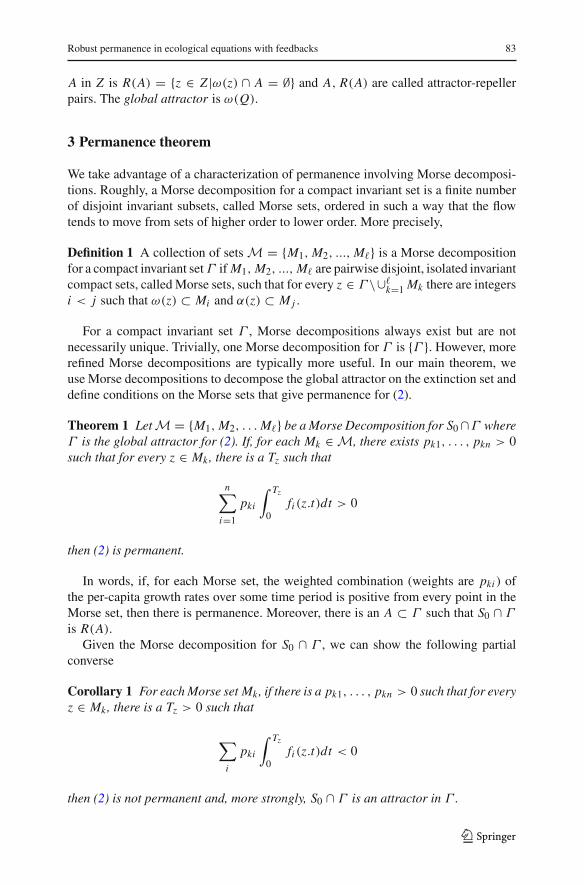
A in Z is R(A) = {z ∈ Z |ω(z) ∩ A = ∅} and A, R(A) are called attractor-repellerpairs. The global attractor is ω(Q).
3 Permanence theorem
We take advantage of a characterization of permanence involving Morse decomposi-tions. Roughly, a Morse decomposition for a compact invariant set is a finite numberof disjoint invariant subsets, called Morse sets, ordered in such a way that the flowtends to move from sets of higher order to lower order. More precisely,
Definition 1 A collection of sets M = {M1, M2, ..., M�} is a Morse decompositionfor a compact invariant setΓ ifM1, M2, ..., M� are pairwise disjoint, isolated invariantcompact sets, called Morse sets, such that for every z ∈ Γ \∪�
k=1 Mk there are integersi < j such that ω(z) ⊂ Mi and α(z) ⊂ Mj .
For a compact invariant set Γ , Morse decompositions always exist but are notnecessarily unique. Trivially, one Morse decomposition for Γ is {Γ }. However, morerefined Morse decompositions are typically more useful. In our main theorem, weuse Morse decompositions to decompose the global attractor on the extinction set anddefine conditions on the Morse sets that give permanence for (2).
Theorem 1 LetM = {M1, M2, . . . M�} be aMorse Decomposition for S0∩Γ whereΓ is the global attractor for (2). If, for each Mk ∈ M, there exists pk1, . . . , pkn > 0such that for every z ∈ Mk, there is a Tz such that
n∑
i=1
pki
∫ Tz
0fi (z.t)dt > 0
then (2) is permanent.
In words, if, for each Morse set, the weighted combination (weights are pki ) ofthe per-capita growth rates over some time period is positive from every point in theMorse set, then there is permanence. Moreover, there is an A ⊂ Γ such that S0 ∩ Γ
is R(A).Given the Morse decomposition for S0 ∩ Γ , we can show the following partial
converse
Corollary 1 For eachMorse set Mk, if there is a pk1, . . . , pkn > 0 such that for everyz ∈ Mk, there is a Tz > 0 such that
∑
i
pki
∫ Tz
0fi (z.t)dt < 0
then (2) is not permanent and, more strongly, S0 ∩ Γ is an attractor in Γ .
123
84 S. Patel, S. J. Schreiber
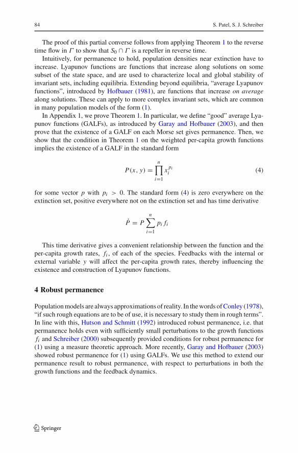
The proof of this partial converse follows from applying Theorem 1 to the reversetime flow in Γ to show that S0 ∩ Γ is a repeller in reverse time.
Intuitively, for permanence to hold, population densities near extinction have toincrease. Lyapunov functions are functions that increase along solutions on somesubset of the state space, and are used to characterize local and global stability ofinvariant sets, including equilibria. Extending beyond equilibria, “average Lyapunovfunctions”, introduced by Hofbauer (1981), are functions that increase on averagealong solutions. These can apply to more complex invariant sets, which are commonin many population models of the form (1).
In Appendix 1, we prove Theorem 1. In particular, we define “good” average Lya-punov functions (GALFs), as introduced by Garay and Hofbauer (2003), and thenprove that the existence of a GALF on each Morse set gives permanence. Then, weshow that the condition in Theorem 1 on the weighted per-capita growth functionsimplies the existence of a GALF in the standard form
P(x, y) =n∏
i=1
x pii (4)
for some vector p with pi > 0. The standard form (4) is zero everywhere on theextinction set, positive everywhere not on the extinction set and has time derivative
P = Pn∑
i=1
pi fi
This time derivative gives a convenient relationship between the function and theper-capita growth rates, fi , of each of the species. Feedbacks with the internal orexternal variable y will affect the per-capita growth rates, thereby influencing theexistence and construction of Lyapunov functions.
4 Robust permanence
Populationmodels are always approximations of reality. In thewords ofConley (1978),“if such rough equations are to be of use, it is necessary to study them in rough terms”.In line with this, Hutson and Schmitt (1992) introduced robust permanence, i.e. thatpermanence holds even with sufficiently small perturbations to the growth functionsfi and Schreiber (2000) subsequently provided conditions for robust permanence for(1) using a measure theoretic approach. More recently, Garay and Hofbauer (2003)showed robust permanence for (1) using GALFs. We use this method to extend ourpermanence result to robust permanence, with respect to perturbations in both thegrowth functions and the feedback dynamics.
123
Robust permanence in ecological equations with feedbacks 85
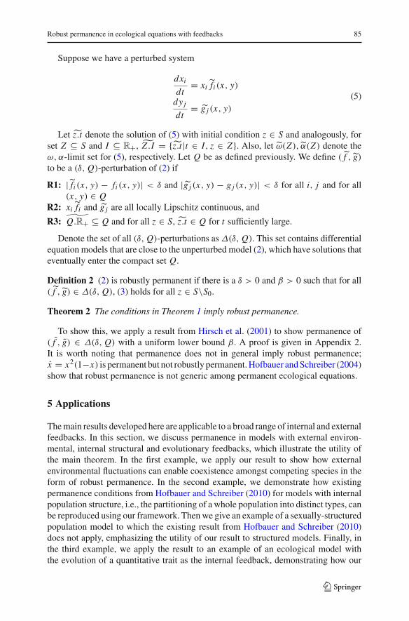
Suppose we have a perturbed system
dxidt
= xi fi (x, y)
dy jdt
= g j (x, y)(5)
Let z.t denote the solution of (5) with initial condition z ∈ S and analogously, forset Z ⊆ S and I ⊆ R+, Z .I = {z.t |t ∈ I, z ∈ Z}. Also, let ω(Z), α(Z) denote theω, α-limit set for (5), respectively. Let Q be as defined previously. We define ( f , g)to be a (δ, Q)-perturbation of (2) if
R1: | fi (x, y) − fi (x, y)| < δ and |g j (x, y) − g j (x, y)| < δ for all i, j and for all(x, y) ∈ Q
R2: xi fi and g j are all locally Lipschitz continuous, and
R3: Q.R+ ⊆ Q and for all z ∈ S, z.t ∈ Q for t sufficiently large.
Denote the set of all (δ, Q)-perturbations as Δ(δ, Q). This set contains differentialequation models that are close to the unperturbed model (2), which have solutions thateventually enter the compact set Q.
Definition 2 (2) is robustly permanent if there is a δ > 0 and β > 0 such that for all( f , g) ∈ Δ(δ, Q), (3) holds for all z ∈ S\S0.Theorem 2 The conditions in Theorem 1 imply robust permanence.
To show this, we apply a result from Hirsch et al. (2001) to show permanence of( f , g) ∈ Δ(δ, Q) with a uniform lower bound β. A proof is given in Appendix 2.It is worth noting that permanence does not in general imply robust permanence;x = x2(1−x) is permanent but not robustly permanent.Hofbauer andSchreiber (2004)show that robust permanence is not generic among permanent ecological equations.
5 Applications
Themain results developed here are applicable to a broad range of internal and externalfeedbacks. In this section, we discuss permanence in models with external environ-mental, internal structural and evolutionary feedbacks, which illustrate the utility ofthe main theorem. In the first example, we apply our result to show how externalenvironmental fluctuations can enable coexistence amongst competing species in theform of robust permanence. In the second example, we demonstrate how existingpermanence conditions from Hofbauer and Schreiber (2010) for models with internalpopulation structure, i.e., the partitioning of a whole population into distinct types, canbe reproduced using our framework. Then we give an example of a sexually-structuredpopulation model to which the existing result from Hofbauer and Schreiber (2010)does not apply, emphasizing the utility of our result to structured models. Finally, inthe third example, we apply the result to an example of an ecological model withthe evolution of a quantitative trait as the internal feedback, demonstrating how our
123
86 S. Patel, S. J. Schreiber
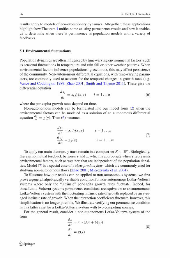
results apply to models of eco-evolutionary dynamics. Altogether, these applicationshighlight how Theorem 1 unifies some existing permanence results and how it enablesus to determine when there is permanence in population models with a variety offeedbacks.
5.1 Environmental fluctuations
Population dynamics are often influenced by time-varying environmental factors, suchas seasonal fluctuations in temperature and rain fall or other weather patterns. Whenenvironmental factors influence populations’ growth rate, this may affect persistenceof the community. Non-autonomous differential equations, with time-varying param-eters, are commonly used to account for the temporal changes in growth rates (e.g.Vance and Coddington 1989; Zhao 2001; Smith and Thieme 2011). These give thedifferential equation
dxidt
= xi fi (x, t) i = 1 . . . n (6)
where the per-capita growth rates depend on time.Non-autonomous models can be formulated into our model form (2) when the
environmental factors can be modeled as a solution of an autonomous differentialequation dy
dt = g(y). Then (6) becomes
dxidt
= xi fi (x, y) i = 1 . . . n
dy jdt
= g j (y) j = 1 . . .m(7)
To apply our main theorem, y must remain in a compact set K ⊂ Rm . Biologically,
there is no mutual feedback between y and x , which is appropriate when y representsenvironmental factors, such as weather, that are independent of the population densi-ties. Model (7) is a special case of a skew product flow, which are commonly used forstudying non-autonomous flows (Zhao 2001; Mierczynski et al. 2004).
To illustrate how our results can be applied to non-autonomous systems, we firstprove a general, algebraically verifiable condition for non-autonomous Lotka–Volterrasystems where only the “intrinsic” per-capita growth rates fluctuate. Indeed, forthese Lotka-Volterra systems permanence conditions are equivalent to an autonomousLotka-Volterra systemwith the fluctuating intrinsic rate of growth replaced by an aver-aged intrinsic rate of growth.When the interaction coefficients fluctuate, however, thissimplification is no longer possible. We illustrate verifying our permanence conditionin this latter case for a Lotka-Volterra system with two competing species.
For the general result, consider a non-autonomous Lotka-Volterra system of theform
dx
dt= x ◦ (Ax + b(y))
dy
dt= g(y)
(8)
123
Robust permanence in ecological equations with feedbacks 87
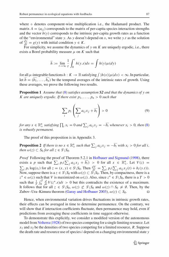
where ◦ denotes component-wise multiplication i.e., the Hadamard product. Thematrix A = (ai j ) corresponds to the matrix of per-capita species interaction strengthsand the vector b(y) corresponds to the intrinsic per-capita growth rates as a functionof the “environmental” state y. As y doesn’t depend on x , we write y.t as the solutionof dy
dt = g(y) with initial condition y ∈ K .For simplicity, we assume the dynamics of y on K are uniquely ergodic, i.e., there
exists a Borel probability measure μ on K such that
h := limt→∞
1
t
∫ t
0h(y.s)ds =
∫
h(y)μ(dy)
for allμ-integrable functionsh : K → R satisfying∫ |h(x)|μ(dx) < ∞. In particular,
let b = (b1, . . . , bn) be the temporal averages of the intrinsic rates of growth. Usingthese averages, we prove the following two results.
Proposition 1 Assume that (8) satisfies assumption S2 and that the dynamics of y onK are uniquely ergodic. If there exist p1, . . . , pn > 0 such that
∑
i
pi
⎛
⎝∑
j
ai j x j + bi
⎞
⎠ > 0 (9)
for any x ∈ Rn+ satisfying
∏i xi = 0 and
∑j ai j x j = −bi whenever xi > 0, then (8)
is robustly permanent.
The proof of this proposition is in Appendix 3.
Proposition 2 If there is no x ∈ Rn+ such that
∑j ai j x j = −bi with xi > 0 for all i ,
then ω(z) ⊂ S0 for all z ∈ S\S0.Proof Following the proof of Theorem 5.2.1 in Hofbauer and Sigmund (1998), thereexists a p such that
∑i pi (
∑j ai j x j + bi ) > 0 for all x ∈ R
n+. Let V (z) =∑
i pi log(xi ) for all z = (x, y) ∈ S\S0. Then dVdt = ∑
i pi (∑
j ai j x j (t) + bi (y.t)).Now, suppose there is a z ∈ S\S0 with ω(z) ⊂ S\S0. Then, by compactness, there is az∗ ∈ ω(z) such that V is maximized on ω(z). Also, since z∗ ∈ S\S0, there is a T > 0such that 1
T
∫ T0
ddt V (z∗.s)dt > 0 but this contradicts the existence of a maximum.
It follows that for all z ∈ S\S0, ω(z) �⊂ S\S0 and ω(z) ∩ S0 �= ∅. Then, by theZubov–Ura–Kimura theorem (Garay and Hofbauer 2003), ω(z) ⊂ S0. ��
Hence, when environmental variation drives fluctuations in intrinsic growth rates,their effects can be averaged in time to determine permanence. On the contrary, wewill show that if interaction coefficients fluctuate, then permanence may hold, even ifpredictions from averaging these coefficients in time suggest otherwise.
To demonstrate this explicitly, we consider a modified version of the autonomousmodel fromVolterra (1928) of two species competing for a single limiting resource. Letx1 and x2 be the densities of two species competing for a limited resource, R. Supposethe death rate and resource use of species i depend on a changing environmental state y
123
88 S. Patel, S. J. Schreiber
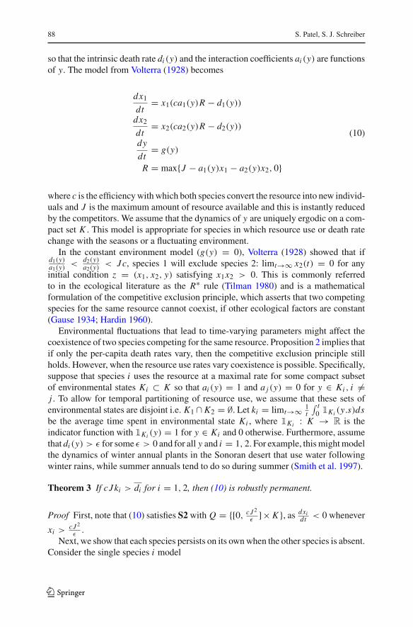
so that the intrinsic death rate di (y) and the interaction coefficients ai (y) are functionsof y. The model from Volterra (1928) becomes
dx1dt
= x1(ca1(y)R − d1(y))
dx2dt
= x2(ca2(y)R − d2(y))
dy
dt= g(y)
R = max{J − a1(y)x1 − a2(y)x2, 0}
(10)
where c is the efficiencywithwhich both species convert the resource into new individ-uals and J is the maximum amount of resource available and this is instantly reducedby the competitors. We assume that the dynamics of y are uniquely ergodic on a com-pact set K . This model is appropriate for species in which resource use or death ratechange with the seasons or a fluctuating environment.
In the constant environment model (g(y) = 0), Volterra (1928) showed that ifd1(y)a1(y)
<d2(y)a2(y)
< Jc, species 1 will exclude species 2: limt→∞ x2(t) = 0 for anyinitial condition z = (x1, x2, y) satisfying x1x2 > 0. This is commonly referredto in the ecological literature as the R∗ rule (Tilman 1980) and is a mathematicalformulation of the competitive exclusion principle, which asserts that two competingspecies for the same resource cannot coexist, if other ecological factors are constant(Gause 1934; Hardin 1960).
Environmental fluctuations that lead to time-varying parameters might affect thecoexistence of two species competing for the same resource. Proposition 2 implies thatif only the per-capita death rates vary, then the competitive exclusion principle stillholds. However, when the resource use rates vary coexistence is possible. Specifically,suppose that species i uses the resource at a maximal rate for some compact subsetof environmental states Ki ⊂ K so that ai (y) = 1 and a j (y) = 0 for y ∈ Ki , i �=j . To allow for temporal partitioning of resource use, we assume that these sets ofenvironmental states are disjoint i.e. K1 ∩ K2 = ∅. Let ki = limt→∞ 1
t
∫ t0 1Ki (y.s)ds
be the average time spent in environmental state Ki , where 1Ki : K → R is theindicator function with 1Ki (y) = 1 for y ∈ Ki and 0 otherwise. Furthermore, assumethat di (y) > ε for some ε > 0 and for all y and i = 1, 2. For example, thismightmodelthe dynamics of winter annual plants in the Sonoran desert that use water followingwinter rains, while summer annuals tend to do so during summer (Smith et al. 1997).
Theorem 3 If cJki > di for i = 1, 2, then (10) is robustly permanent.
Proof First, note that (10) satisfies S2 with Q = {[0, cJ 2ε
]× K }, as dxidt < 0 whenever
xi > cJ 2ε
.
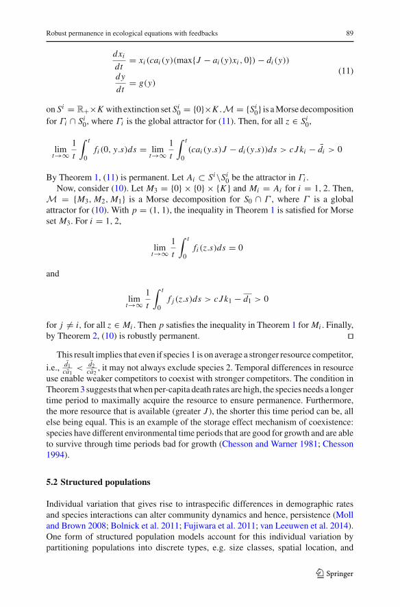
Next, we show that each species persists on its ownwhen the other species is absent.Consider the single species i model
123
Robust permanence in ecological equations with feedbacks 89
dxidt
= xi (cai (y)(max{J − ai (y)xi , 0}) − di (y))
dy
dt= g(y)
(11)
on Si = R+×K with extinction set Si0 = {0}×K .M = {Si0} is aMorse decompositionfor Γi ∩ Si0, where Γi is the global attractor for (11). Then, for all z ∈ Si0,
limt→∞
1
t
∫ t
0fi (0, y.s)ds = lim
t→∞1
t
∫ t
0(cai (y.s)J − di (y.s))ds > cJki − di > 0
By Theorem 1, (11) is permanent. Let Ai ⊂ Si\Si0 be the attractor in Γi .Now, consider (10). Let M3 = {0} × {0} × {K } and Mi = Ai for i = 1, 2. Then,
M = {M3, M2, M1} is a Morse decomposition for S0 ∩ Γ , where Γ is a globalattractor for (10). With p = (1, 1), the inequality in Theorem 1 is satisfied for Morseset M3. For i = 1, 2,
limt→∞
1
t
∫ t
0fi (z.s)ds = 0
and
limt→∞
1
t
∫ t
0f j (z.s)ds > cJk1 − d1 > 0
for j �= i, for all z ∈ Mi . Then p satisfies the inequality in Theorem 1 for Mi . Finally,by Theorem 2, (10) is robustly permanent. ��
This result implies that even if species 1 is on average a stronger resource competitor,
i.e., d1ca1
< d2ca2
, it may not always exclude species 2. Temporal differences in resourceuse enable weaker competitors to coexist with stronger competitors. The condition inTheorem3 suggests thatwhenper-capita death rates are high, the species needs a longertime period to maximally acquire the resource to ensure permanence. Furthermore,the more resource that is available (greater J ), the shorter this time period can be, allelse being equal. This is an example of the storage effect mechanism of coexistence:species have different environmental time periods that are good for growth and are ableto survive through time periods bad for growth (Chesson and Warner 1981; Chesson1994).
5.2 Structured populations
Individual variation that gives rise to intraspecific differences in demographic ratesand species interactions can alter community dynamics and hence, persistence (Molland Brown 2008; Bolnick et al. 2011; Fujiwara et al. 2011; van Leeuwen et al. 2014).One form of structured population models account for this individual variation bypartitioning populations into discrete types, e.g. size classes, spatial location, and
123
90 S. Patel, S. J. Schreiber
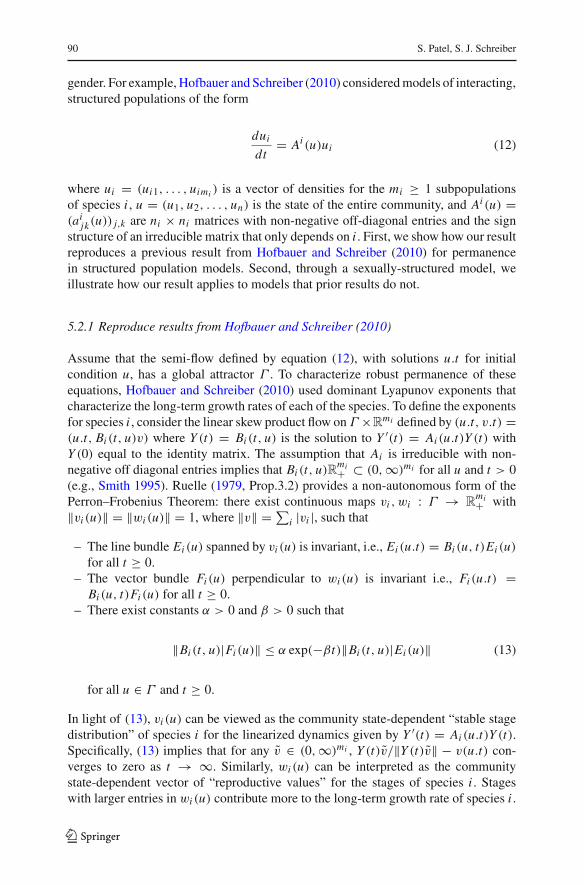
gender. For example, Hofbauer and Schreiber (2010) consideredmodels of interacting,structured populations of the form
duidt
= Ai (u)ui (12)
where ui = (ui1, . . . , uimi ) is a vector of densities for the mi ≥ 1 subpopulationsof species i , u = (u1, u2, . . . , un) is the state of the entire community, and Ai (u) =(aijk(u)) j,k are ni × ni matrices with non-negative off-diagonal entries and the signstructure of an irreducible matrix that only depends on i . First, we show how our resultreproduces a previous result from Hofbauer and Schreiber (2010) for permanencein structured population models. Second, through a sexually-structured model, weillustrate how our result applies to models that prior results do not.
5.2.1 Reproduce results from Hofbauer and Schreiber (2010)
Assume that the semi-flow defined by equation (12), with solutions u.t for initialcondition u, has a global attractor Γ . To characterize robust permanence of theseequations, Hofbauer and Schreiber (2010) used dominant Lyapunov exponents thatcharacterize the long-term growth rates of each of the species. To define the exponentsfor species i , consider the linear skew product flow on Γ ×R
mi defined by (u.t, v.t) =(u.t, Bi (t, u)v) where Y (t) = Bi (t, u) is the solution to Y ′(t) = Ai (u.t)Y (t) withY (0) equal to the identity matrix. The assumption that Ai is irreducible with non-negative off diagonal entries implies that Bi (t, u)R
mi+ ⊂ (0,∞)mi for all u and t > 0(e.g., Smith 1995). Ruelle (1979, Prop.3.2) provides a non-autonomous form of thePerron–Frobenius Theorem: there exist continuous maps vi , wi : Γ → R
mi+ with‖vi (u)‖ = ‖wi (u)‖ = 1, where ‖v‖ = ∑
i |vi |, such that
– The line bundle Ei (u) spanned by vi (u) is invariant, i.e., Ei (u.t) = Bi (u, t)Ei (u)
for all t ≥ 0.– The vector bundle Fi (u) perpendicular to wi (u) is invariant i.e., Fi (u.t) =
Bi (u, t)Fi (u) for all t ≥ 0.– There exist constants α > 0 and β > 0 such that
‖Bi (t, u)|Fi (u)‖ ≤ α exp(−βt)‖Bi (t, u)|Ei (u)‖ (13)
for all u ∈ Γ and t ≥ 0.
In light of (13), vi (u) can be viewed as the community state-dependent “stable stagedistribution” of species i for the linearized dynamics given by Y ′(t) = Ai (u.t)Y (t).Specifically, (13) implies that for any v ∈ (0,∞)mi , Y (t)v/‖Y (t)v‖ − v(u.t) con-verges to zero as t → ∞. Similarly, wi (u) can be interpreted as the communitystate-dependent vector of “reproductive values” for the stages of species i . Stageswith larger entries in wi (u) contribute more to the long-term growth rate of species i .
123
Robust permanence in ecological equations with feedbacks 91
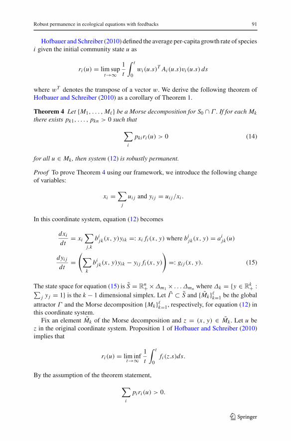
Hofbauer and Schreiber (2010) defined the average per-capita growth rate of speciesi given the initial community state u as
ri (u) = lim supt→∞
1
t
∫ t
0wi (u.s)T Ai (u.s)vi (u.s) ds
where wT denotes the transpose of a vector w. We derive the following theorem ofHofbauer and Schreiber (2010) as a corollary of Theorem 1.
Theorem 4 Let {M1, . . . , M�} be a Morse decomposition for S0 ∩ Γ . If for each Mk
there exists pk1, . . . , pkn > 0 such that
∑
i
pki ri (u) > 0 (14)
for all u ∈ Mk, then system (12) is robustly permanent.
Proof To prove Theorem 4 using our framework, we introduce the following changeof variables:
xi =∑
j
ui j and yi j = ui j/xi .
In this coordinate system, equation (12) becomes
dxidt
= xi∑
j,k
bijk(x, y)yik =: xi fi (x, y) where bijk(x, y) = aijk(u)
dyi jdt
=(
∑
k
bijk(x, y)yik − yi j fi (x, y)
)
=: gi j (x, y). (15)
The state space for equation (15) is S = Rn+ ×Δm1 × . . . Δmn where Δk = {y ∈ R
k+ :∑
j y j = 1} is the k − 1 dimensional simplex. Let Γ ⊂ S and {Mk}�k=1 be the global
attractor Γ and the Morse decomposition {Mk}�k=1, respectively, for equation (12) inthis coordinate system.
Fix an element Mk of the Morse decomposition and z = (x, y) ∈ Mk . Let u bez in the original coordinate system. Proposition 1 of Hofbauer and Schreiber (2010)implies that
ri (u) = lim inft→∞
1
t
∫ t
0fi (z.s)ds.
By the assumption of the theorem statement,
∑
i
pi ri (u) > 0.
123
92 S. Patel, S. J. Schreiber
Hence, we can choose Tz > 0 such that
∑
i
pi
∫ Tz
0fi (z.s)ds > 0.
Applying Theorem 1 completes the proof. ��The change of variables from (12) to (15) demonstrates how structured populations
can be reformulated into our general framework and reproduce results from Hofbauerand Schreiber (2010).
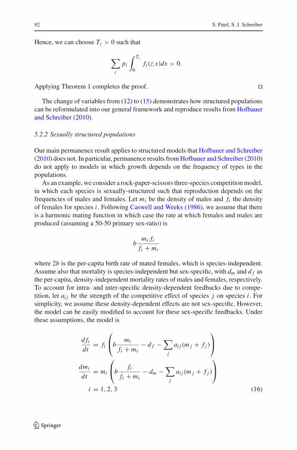
5.2.2 Sexually structured populations
Our main permanence result applies to structured models that Hofbauer and Schreiber(2010) does not. In particular, permanence results fromHofbauer and Schreiber (2010)do not apply to models in which growth depends on the frequency of types in thepopulations.
As an example, we consider a rock-paper-scissors three-species competitionmodel,in which each species is sexually-structured such that reproduction depends on thefrequencies of males and females. Let mi be the density of males and fi the densityof females for species i . Following Caswell and Weeks (1986), we assume that thereis a harmonic mating function in which case the rate at which females and males areproduced (assuming a 50-50 primary sex-ratio) is
bmi fifi + mi
where 2b is the per-capita birth rate of mated females, which is species-independent.Assume also that mortality is species-independent but sex-specific, with dm and d f asthe per-capita, density-independent mortality rates of males and females, respectively.To account for intra- and inter-specific density-dependent feedbacks due to compe-tition, let ai j be the strength of the competitive effect of species j on species i . Forsimplicity, we assume these density-dependent effects are not sex-specific. However,the model can be easily modified to account for these sex-specific feedbacks. Underthese assumptions, the model is
d fidt
= fi
⎛
⎝bmi
fi + mi− d f −
∑
j
ai j (m j + f j )
⎞
⎠
dmi
dt= mi
⎛
⎝bfi
fi + mi− dm −
∑
j
ai j (m j + f j )
⎞
⎠
i = 1, 2, 3 (16)
123
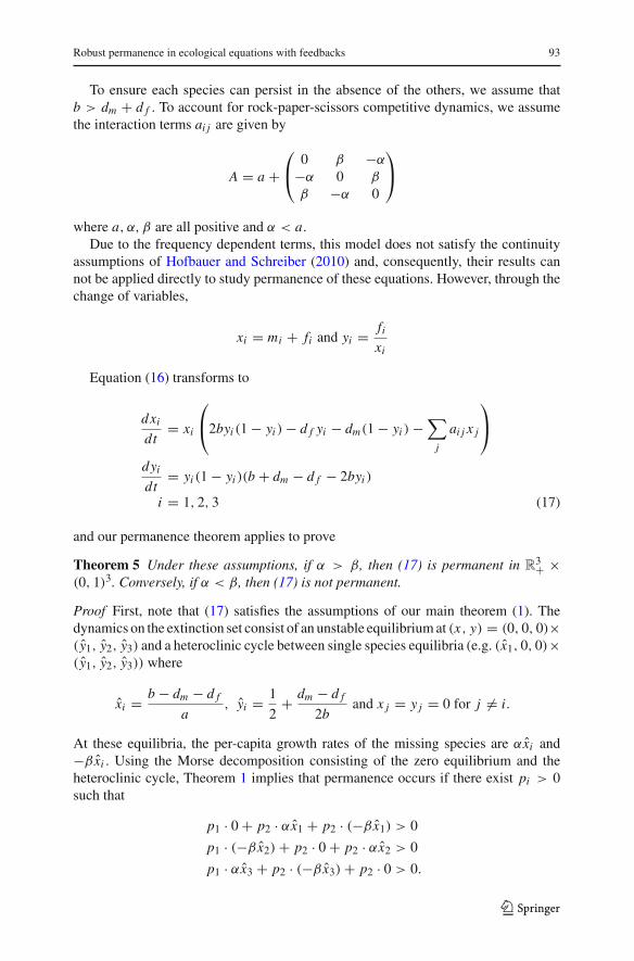
Robust permanence in ecological equations with feedbacks 93
To ensure each species can persist in the absence of the others, we assume thatb > dm + d f . To account for rock-paper-scissors competitive dynamics, we assumethe interaction terms ai j are given by
A = a +⎛
⎝0 β −α
−α 0 β
β −α 0
⎞
⎠
where a, α, β are all positive and α < a.Due to the frequency dependent terms, this model does not satisfy the continuity
assumptions of Hofbauer and Schreiber (2010) and, consequently, their results cannot be applied directly to study permanence of these equations. However, through thechange of variables,
xi = mi + fi and yi = fixi
Equation (16) transforms to
dxidt
= xi
⎛
⎝2byi (1 − yi ) − d f yi − dm(1 − yi ) −∑
j
ai j x j
⎞
⎠
dyidt
= yi (1 − yi )(b + dm − d f − 2byi )
i = 1, 2, 3 (17)
and our permanence theorem applies to prove
Theorem 5 Under these assumptions, if α > β, then (17) is permanent in R3+ ×
(0, 1)3. Conversely, if α < β, then (17) is not permanent.
Proof First, note that (17) satisfies the assumptions of our main theorem (1). Thedynamics on the extinction set consist of an unstable equilibriumat (x, y) = (0, 0, 0)×(y1, y2, y3) and a heteroclinic cycle between single species equilibria (e.g. (x1, 0, 0)×(y1, y2, y3)) where
xi = b − dm − d f
a, yi = 1
2+ dm − d f
2band x j = y j = 0 for j �= i.
At these equilibria, the per-capita growth rates of the missing species are α xi and−β xi . Using the Morse decomposition consisting of the zero equilibrium and theheteroclinic cycle, Theorem 1 implies that permanence occurs if there exist pi > 0such that
p1 · 0 + p2 · α x1 + p2 · (−β x1) > 0
p1 · (−β x2) + p2 · 0 + p2 · α x2 > 0
p1 · α x3 + p2 · (−β x3) + p2 · 0 > 0.
123
94 S. Patel, S. J. Schreiber
As x1 = x2 = x3, there is a solution to these linear inequalities if and only if α > β.Conversely, there is a solution to the reversed linear inequalities if and only if β > α
and then Theorem 1 implies that (17) is not permanent. ��
Theorem 5 yields the same permanence condition as in the classic asexual model.Due to our assumption that density-dependent feedbacks are not sex-specific, thesystem is only partially coupled as the frequency dynamics of y do not depend onx . With sex-specific density-dependent feedbacks, the system would be fully coupledbut still analytically tractable as these feedbacks would appear as linear functions ofxi in the yi equations.
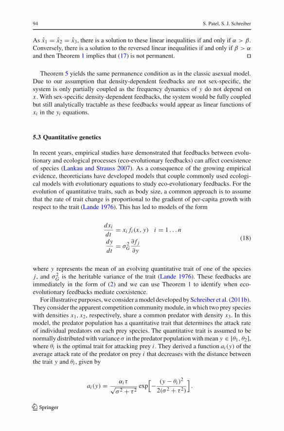
5.3 Quantitative genetics
In recent years, empirical studies have demonstrated that feedbacks between evolu-tionary and ecological processes (eco-evolutionary feedbacks) can affect coexistenceof species (Lankau and Strauss 2007). As a consequence of the growing empiricalevidence, theoreticians have developed models that couple commonly used ecologi-cal models with evolutionary equations to study eco-evolutionary feedbacks. For theevolution of quantitative traits, such as body size, a common approach is to assumethat the rate of trait change is proportional to the gradient of per-capita growth withrespect to the trait (Lande 1976). This has led to models of the form
dxidt
= xi fi (x, y) i = 1 . . . n
dy
dt= σ 2
G∂ f j∂y
(18)
where y represents the mean of an evolving quantitative trait of one of the speciesj , and σ 2
G is the heritable variance of the trait (Lande 1976). These feedbacks areimmediately in the form of (2) and we can use Theorem 1 to identify when eco-evolutionary feedbacks mediate coexistence.
For illustrative purposes,we consider amodel developed bySchreiber et al. (2011b).They consider the apparent competition communitymodule, inwhich two prey specieswith densities x1, x2, respectively, share a common predator with density x3. In thismodel, the predator population has a quantitative trait that determines the attack rateof individual predators on each prey species. The quantitative trait is assumed to benormally distributedwith varianceσ in the predator populationwithmean y ∈ [θ1, θ2],where θi is the optimal trait for attacking prey i . They derived a function ai (y) of theaverage attack rate of the predator on prey i that decreases with the distance betweenthe trait y and θi , given by
ai (y) = αiτ√σ 2 + τ 2
exp[− (y − θi )
2
2(σ 2 + τ 2)
].
123
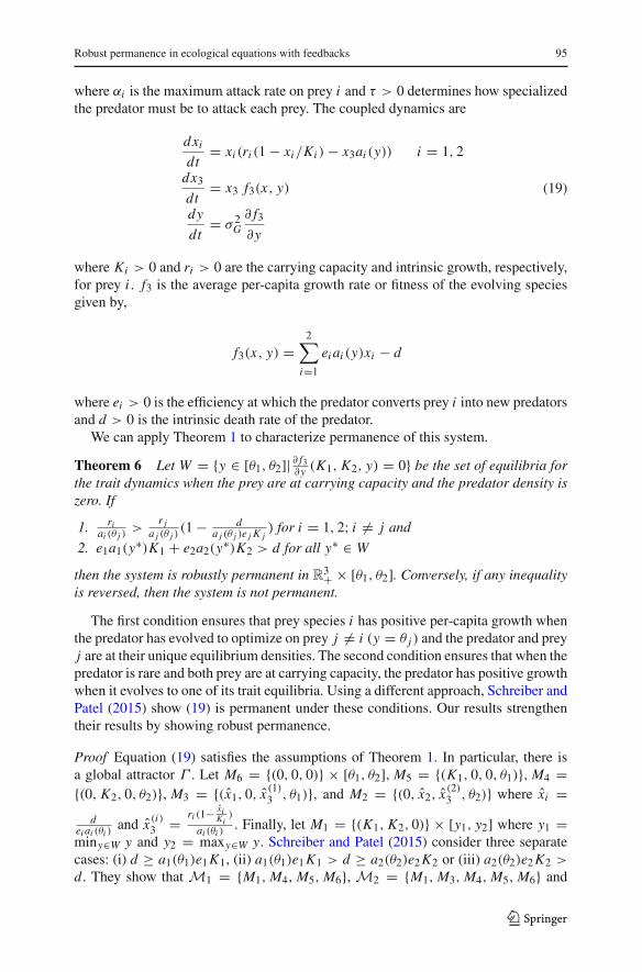
Robust permanence in ecological equations with feedbacks 95
where αi is the maximum attack rate on prey i and τ > 0 determines how specializedthe predator must be to attack each prey. The coupled dynamics are
dxidt
= xi (ri (1 − xi/Ki ) − x3ai (y)) i = 1, 2
dx3dt
= x3 f3(x, y)
dy
dt= σ 2
G∂ f3∂y
(19)
where Ki > 0 and ri > 0 are the carrying capacity and intrinsic growth, respectively,for prey i . f3 is the average per-capita growth rate or fitness of the evolving speciesgiven by,
f3(x, y) =2∑
i=1
eiai (y)xi − d
where ei > 0 is the efficiency at which the predator converts prey i into new predatorsand d > 0 is the intrinsic death rate of the predator.
We can apply Theorem 1 to characterize permanence of this system.
Theorem 6 Let W = {y ∈ [θ1, θ2]| ∂ f3∂y (K1, K2, y) = 0} be the set of equilibria for
the trait dynamics when the prey are at carrying capacity and the predator density iszero. If
1. riai (θ j )
>r j
a j (θ j )(1 − d
a j (θ j )e j K j) for i = 1, 2; i �= j and
2. e1a1(y∗)K1 + e2a2(y∗)K2 > d for all y∗ ∈ W
then the system is robustly permanent in R3+ × [θ1, θ2]. Conversely, if any inequality
is reversed, then the system is not permanent.
The first condition ensures that prey species i has positive per-capita growth whenthe predator has evolved to optimize on prey j �= i (y = θ j ) and the predator and preyj are at their unique equilibrium densities. The second condition ensures that when thepredator is rare and both prey are at carrying capacity, the predator has positive growthwhen it evolves to one of its trait equilibria. Using a different approach, Schreiber andPatel (2015) show (19) is permanent under these conditions. Our results strengthentheir results by showing robust permanence.
Proof Equation (19) satisfies the assumptions of Theorem 1. In particular, there isa global attractor Γ . Let M6 = {(0, 0, 0)} × [θ1, θ2], M5 = {(K1, 0, 0, θ1)}, M4 ={(0, K2, 0, θ2)}, M3 = {(x1, 0, x (1)
3 , θ1)}, and M2 = {(0, x2, x (2)3 , θ2)} where xi =
dei ai (θi )
and x (i)3 = ri (1− xi
Ki)
ai (θi ). Finally, let M1 = {(K1, K2, 0)} × [y1, y2] where y1 =
miny∈W y and y2 = maxy∈W y. Schreiber and Patel (2015) consider three separatecases: (i) d ≥ a1(θ1)e1K1, (ii) a1(θ1)e1K1 > d ≥ a2(θ2)e2K2 or (iii) a2(θ2)e2K2 >
d. They show that M1 = {M1, M4, M5, M6}, M2 = {M1, M3, M4, M5, M6} and
123
96 S. Patel, S. J. Schreiber
M3 = {M1, M2, M3, M4, M5, M6} form a Morse decomposition for (19) under case(i), (ii), and (iii) restricted to Γ ∩ S0, respectively.
Consider case (iii). For each Morse set Mk ∈ M3, there exist a vector pk thatsatisfies the inequality in Theorem 1 for every point in the set. For example, for ε
sufficiently small, p6 = (1, 1, ε) satisfies the inequality in Theorem 1 for M6. Case(ii) and case (i) follow similarly. ��
6 Discussion
Understanding how abiotic and biotic factors determine coexistence of interactingspecies is a fundamental problem in ecology. Ecologists have demonstrated that factorsinternal to the populations, such as individual variation (Bolnick et al. 2011;Violle et al.2012;Hart et al. 2016;Barabás andD’Andrea 2016) and evolution (Lankau andStrauss2007; Barabás and D’Andrea 2016), and factors external to the populations, such astemporal variation in abiotic factors (Hutchinson 1961), can have substantial impactson population dynamics. Moreover, as these internal and external factors change, theirinfluence on population growth leads to changes in population densities which in turnmay alter these factors, thereby creating a feedback loop. The instrumental role ofthis feedback on coexistence has been demonstrated both empirically (e.g. Lankauand Strauss 2007; Chung and Rudgers 2016) as well as theoretically (e.g. Bever et al.1997; Revilla et al. 2013). Our work develops the mathematical framework for findingconditions that enable coexistence in community dynamicmodels with feedbacks and,by applying this theory, elucidates the role of these internal and external feedbacks oncoexistence.
We find that if there is a weighting of the species such that the temporal average ofthe weighted per-capita growth rates is positive whenever a species is missing, thenpopulations coexist with feedbacks. Moreover, given a Morse decomposition for theextinction set, these weightings can differ among the components of this decomposi-tion. For models without feedbacks, this sufficient condition for robust permanence isequivalent to the condition found by Garay and Hofbauer (2003). Hence, our resultsprovide a natural extension to models with internal and external feedbacks. As ourexamples illustrate, these feedbacks play two critical roles for coexistence. First, theeffect of the feedback variable will influence the Morse decomposition for the extinc-tion set. Second, feedbacks affect the per-capita growth of each of the species andthereby, influence whether the weighted combination of these growth rates can bepositive. These differences can drive feedbacks to enable or prevent coexistence.
In addition to extending the work of Garay and Hofbauer (2003) to include internaland external feedbacks, our general framework and permanence result incorporatesexisting population models with specific types of internal feedbacks (Caswell andWeeks 1986; Caswell 2001; Hofbauer and Schreiber 2010), external feedbacks (Arm-strong and McGehee 1976; Mottoni and Schiaffino 1981; Zhao 2001), and mixturesof internal and external feedbacks (Hastings et al. 2007; Cuddington et al. 2009).Through our examples, we illustrate how to transform several of these earlier resultsinto our framework. In our first example, we formulate a non-autonomous modelwith parameters that vary with the environment into our framework by introducing
123

Robust permanence in ecological equations with feedbacks 97
a feedback variable that models the dynamics of the environmental variation. In thesecond example, we transform a structured population model, in which populationsare partitioned into distinct types, into our framework, via a change of variables intofrequencies of types and total densities. The frequencies of the different types withinthe population act as the internal feedback variables. Finally, in the third example,we demonstrate how our results apply to population models with feedbacks due totrait evolution. These examples highlight that our framework can help elucidate howpopulations coexist in a range of ecological scenarios.
In an attempt to explain empirical evidence for coexistence that was incompat-ible with theoretical predictions, Hutchinson (1961) postulates that changes in theenvironment that alter the competitive superiority of one species over another canenable coexistence. Our first example highlights that ergodic environmental varia-tion that drives temporal differences in ecological parameters can enable coexistenceof populations in a community, but that this depends on the role it has on influ-encing population growth. In particular, we show that environmental variation thatinfluences species interactions enables coexistence, in comparison to an analogousmodel that uses time-averaged parameters instead of explicitly accounting for varia-tion. Our results are an extension of previous work that showed coexistence amongsttwo competing species with periodic environmental variation (Armstrong and McGe-hee 1976; Cushing 1980; Mottoni and Schiaffino 1981) and a specification of thegeneral results for non-autonomous two species models (Zhao 2001). Notably, ourexample demonstrates how variation and separation of resource use between twospecies can enable coexistence through a storage effect (Chesson and Warner 1981),provided that species are “stored” through periods they do not use the resource andcan sufficiently recover through periods in which they do. Interestingly, our resultsalso highlight that environmental variation that only influences non-interaction terms,such as per-capita mortality, does not enable coexistence due to the linearity of non-interaction terms in the model. The necessity for temporal variation to act in nonlinearways to enable coexistence was also noted for models with stochastic environments(Schreiber 2010) as well as in discrete time models with non-overlapping generations(Chesson and Warner 1981; Chesson 1994).
In addition to externally-driven temporal variation, internal variation within popu-lations may also impact coexistence. Many reviews highlight that models with internalvariation can lead to different predictions and inferences in both empirical and theoret-ical ecological studies compared tomean fieldmodels (Bolnick et al. 2011; Violle et al.2012; Hart et al. 2016). Structured population models, a commonly used frameworkfor accounting for internal variation, involve partitioning the population into distincttypes, such as based on sex, life stages, or location in space, so that each type hasits own growth rate depending on all other types (Caswell and Weeks 1986; Caswell2001). Our permanence condition can be used to determine when structured interact-ing populations coexist. These results apply to structured models that previous resultsfrom Hofbauer and Schreiber (2010) do not. Mainly, Hofbauer and Schreiber (2010)made two mathematical assumptions. First, they assume that there were no negativeinteractions between individuals of different types. This assumption may not holdin a number of common ecological scenarios, including models with cannibalism orother forms of interference, which is a prevalent negative interaction between different
123
98 S. Patel, S. J. Schreiber
life stages within a population (Fox 1975; Polis 1981). Second, they assume conti-nuity in the growth matrices Ai , which restricts their framework to models with nofrequency dependent growth. Growth in structured models may be frequency depen-dent in a number of biological scenarios. In our example, we apply our results to asexually-structuredmodel,which, followingCaswell andWeeks (1986), has frequencydependence since fecundity depends on sex ratios. In particular, through a change ofvariable from the densities of different types within a species to total density and fre-quency of types, structured models can be reformulated into our framework, makingthe permanence conditions applicable to a broad range of structured models.
When individual variation in a population is heritable, this sets the stage for evo-lution to take place in response to differential selection pressures (Violle et al. 2012).Recent empirical evidence has demonstrated the prevalence of feedbacks betweenpopulation dynamics and trait evolution (called eco-evolutionary feedbacks; reviewedin Schoener 2011; Lankau and Strauss 2011 and that these feedbacks may impactpopulation dynamics (Abrams 2000; Lankau 2009; Cortez and Ellner 2010; Vasseuret al. 2011; Schreiber et al. 2011b; Northfield and Ives 2013; Patel and Schreiber2015). Thus far, few studies have shown permanence in these types of models (but see(Schreiber et al. 2011b; Schreiber and Patel 2015)), and we hope that these results willmotivate analyses of coexistence in the sense of permanence in future eco-evolutionarystudies. Through our example, we demonstrate how these results can elucidate the con-ditions for robust permanence in a model where a predator is evolving between traitsthat are more fit for attacking one prey species versus another. In the absence of eco-evolutionary feedbacks, the prey species exhibit apparent competition: increasing thedensity of one prey increases the predator density and, thereby, results in a reductionof the other prey species (Holt 1977). For highly enriched environments in which thecarrying capacities of the prey are large, this apparent competition can lead to exclu-sion of one of the prey species (Holt and Lawton 1994). As the predator evolves tospecialize on the more common prey, eco-evolutionary feedbacks can rescue the rareprey from this outcome and enable coexistence. Applying our results to other eco-evolutionary models may provide opportunities to gain a more general understandingof the role of evolution on species coexistence.
Our results here extend existingmethods for permanence to account for internal andexternal feedbacks, generalizing some existing results and broadening their applicabil-ity. There are a number of natural avenues that would be useful to develop in the future,including infinite dimensional models and stochastic models. We assume feedbacksare contained inR
m+. However, some internal and external feedbacksmay be better cap-tured in infinite dimensions and extending our results to account for this may be useful(e.g. integral projection models; Easterling et al. 2000). Permanence has been studiedin general infinite dimensional dynamical systems (Hale and Waltman 1989; Smithand Thieme 2011) as well as in models with specific types of feedbacks, includingthose captured through continuous spatial heterogeneity (Dunbar et al. 1986; Cantrellet al. 1993, 1996; Zhao and Hutson 1994; Furter and López-Gómez 1997; Cantrelland Cosner 2003; Zhao 2003; Mierczynski et al. 2004; Smith and Thieme 2011),age structure (Smith and Thieme 2011) and time delays (Burton and Hutson 1989;Freedman and Ruan 1995; Ruan and Zhao 1999; Zhao 2003). Whether transformingthese models into a framework analogous to the one here is useful requires further
123
Robust permanence in ecological equations with feedbacks 99
exploration. Furthermore, populations may feedback with random internal or externalfactors. Extending permanence results for stochastic population models to account forfeedbacks will enable comparisons to our framework to understand broadly the roleof random feedbacks on coexistence. With the growing number of empirical studiesinvestigating internal and external factors that influence population dynamics, eco-logical models are becoming more sophisticated. In order for permanence to remainan important concept in ecology, the methods for demonstrating permanence mustcontinue to expand to these new modeling frameworks.
Acknowledgements Open access funding provided by University of Vienna. Financial support by the U.S.National Science Foundation Grant DMS-1313418 to SJS, the American Association of University WomenDissertation Fellowship to SP and the Austrian Science Fund (FWF) Grant P25188-N25 to Reinhard Burgerat the University of Vienna is gratefully acknowledged.
Open Access This article is distributed under the terms of the Creative Commons Attribution 4.0 Interna-tional License (http://creativecommons.org/licenses/by/4.0/), which permits unrestricted use, distribution,and reproduction in any medium, provided you give appropriate credit to the original author(s) and thesource, provide a link to the Creative Commons license, and indicate if changes were made.
Appendix 1: Proof of Theorem 1
To prove Theorem 1, we begin by introducing “good average Lyapunov functions”and proving a more general theorem.
Definition A1 A continuous map P : U → R, whereU ⊂ S is an open set, is a goodaverage Lyapunov function (GALF) for (2) if
– P(z) = 0 for all z ∈ S0 ∩U and P(z) > 0 for all z ∈ (S\S0) ∩U ,– P is differentiable on (S\S0) ∩U ,– ∂P
∂y j= 0 for all j ,
– pi := xiP
∂P∂xi
, which are continuous functions defined on (S\S0) ∩ U and extendcontinuously to S ∩U , and
– for every z ∈ S0 ∩U , there is a Tz > 0 such that z.t ∈ U for t ∈ [0, Tz], and∫ Tz
0
∑
i
pi (z.t) fi (z.t)dt > 0.
We prove the following theorem
Theorem A1 Let M = {M1, M2, . . . M�} be a Morse decomposition for S0 ∩ Γ of(2). For each k, let Uk be an open neighborhood of Mk and let Pk : Uk → R be agood average Lyapunov function for (2). Then (2) is permanent.
Proof Fix k. Let F(z, T ) := ∫ T0
∑i pi (z.t) fi (z.t)dt for all z ∈ Uk and T ≥ 0, where
pi is defined from the definition of a GALF.By definition of the GALF, for all z ∈ Mk , there is a Tz > 0 and δ(z) > 0 such that
F(z, Tz) > δ(z)
123
100 S. Patel, S. J. Schreiber
By continuity of F , there is a neighborhood Vz ⊂ Uk of z ∈ Mk such thatF(v, Tz) >
δ(z)2 for all v ∈ Vz . The collection of sets {Vz}z∈Mk forms an open cover
of Mk . By compactness, there is a finite subcover {Vz j }�j=1. Let Vk = ∪�j=1Vz j , c =
12 min{δ(z j )}�j=1 and T = max{Tj }�j=1, where Tj := Tz j .
Then, Vk ⊂ Uk is a neighborhood of Mk such that for all z ∈ Vk there is a0 < Tj < T satisfying
F(z, Tj ) > c.
Furthermore, for z ∈ (S\S0) ∩ Vk ,
ln(P(z.Tj )) − ln(P(z)) =∫ Tj
0
1
P(z.s)
d
dsP(z.s)ds
=∫ Tj
0
1
P(z.s)
(n∑
i=1
∂P
∂xi
dxids
+m∑
i=1
∂P
∂yi
dyids
)
ds
=∫ Tj
0
n∑
i=1
pi (z.s) fi (z.s)ds > c,
which givesP(z(Tj )) > (1 + c)P(z). (A1)
By the Corollary to Theorem 2 fromGaray (1989), permanence follows from show-ing that each Mk is isolated and that (S\S0) ∩ Ws(Mk) = ∅, where Ws(Mk) = {z ∈S|∅ �= ω(z) ⊂ Mk}. For any initial condition z, let γ +(z) = z.[0,∞) be the forwardtrajectory of z. Assume there is a z ∈ (S\S0)∩Vk such that γ +(z) ⊆ Vk . Then, there isa z∗ ∈ γ +(z)∩Vk such that P(z∗) = max
v∈γ +(z)∩Vk P(v). Then, either (i) there existsa t∗ > 0 such that z∗ = z.t∗ or (ii) there exists tn → ∞ such that zn := z.tn convergesto z∗ as n → ∞. If (i), then equation (A1) implies P(z∗.Tz∗) > (1 + c)P(z∗) forsome Tz∗ > 0, which is a contradiction to the choice of z∗ since z∗.Tz∗ ∈ γ +(v). If(ii), then for some sequence Tzn > 0, P(zn .Tzn ) > (1 + c)P(zn) → (1 + c)P(z∗),which is a contradiction to the choice of z∗ since zn .Tzn ∈ γ +(z) for all n.
Hence, for all v ∈ (S\S0) ∩ Vk , γ +(v)\Vk �= ∅. It follows that Mk is isolated andfor all v ∈ (S\S0) ∩ Vk , ω(v) �⊂ Mk . The latter gives that (S\S0) ∩ Ws(Mk) = ∅. ��
Theorem 1 immediately follows when using the standard form (4) as a GALF oneach Morse set. It is easy to see that when pki > 0 for all i, k, (4) satisfies the firstfour properties of a GALF. In particular, the fourth and fifth property follow sincexiP
∂P∂xi
= pki and hence is constant in U .
Appendix 2: Proof of Theorem 2
To show robust permanence, we will use the following theorem from Hirsch et al.(2001) [Corollary 4.5]. Note that this corollary is for maps, but an analogous proof forflows holds (see Hirsch et al. 2001 [Remark 4.6]).
123
Robust permanence in ecological equations with feedbacks 101
Theorem A2 Let (S, d) and (Λ, ρ) be metric spaces. For each λ ∈ Λ, let φλ :S × R → S be a flow that is continuous in λ, z, t . Let Sp ⊂ S be an open subset suchthat Sp is invariant for all λ and let ∂S = S\Sp. Also, assume that every forwardtrajectory for φλ has compact closure in S and that
⋃λ∈Λ,z∈S ωλ(z) has compact
closure, where ωλ denotes the ω-limit for φλ. Let λ0 ∈ Λ be fixed and assume that
T1: φλ0 hasaglobal attractorΓ and there exists aMorsedecomposition {M1, . . . , M�}for Γ ∩ ∂S
T2: there exists δ0 > 0 such that for any λ ∈ Λ with ρ(λ, λ0) < δ0 and any z ∈ Sp,lim supt→∞ d(φλ(z, t), Mk) ≥ δ0, for all 1 ≤ k ≤ �.
Then, there exists a β > 0 and δ > 0 such that lim inf t→∞ d(φλ(z, t), ∂S) ≥ β
for any λ ∈ Λ with ρ(λ, λ0) < δ and any z ∈ Sp.
To apply this theorem, endow Λ = Δ(1, Q) with the sup norm (i.e. ρ(h1, h2) =‖(h1, h2)‖∞ = supz∈Q ‖h1(z), h2(z)‖). Let S = R
n+m with the standard metric andlet Sp = S\S0. By R3 in the definition of perturbations, ⋃( f ,g)∈Δ(1,Q),z∈S ω(z) ⊂ Qand so has compact closure. For ( f, g), we have a Morse decomposition for Γ ∩ S0.
Hence, we only have to show T2. To do this, we show that there exists a 1 > δ > 0sufficiently small such that if Pk is a GALF onUk for (2), then it is also a GALF on Vkfor every ( f , g) ∈ Δ(δ, Q), where Vk is defined in the proof of Theorem 1. First, notethat the first four conditions defining a GALF are properties of P and independent ofthe flow. Hence, these are still satisfied. We must show the final condition: for a δ > 0sufficiently small, for all z ∈ Vk ∩ S0, there is a Tz > 0 such that
∫ Tz
0
n∑
i=1
pi (z.t) fi (z.t)dt > 0 (A2)
for every ( f , g) ∈ Δ(δ, Q).Let F(z, T ) := ∫ T
0
∑i pi (z.t) fi (z.t)dt and F(z, T ) := ∫ T
0
∑i pi (z.t) fi (z.t)dt .
Let T, c be such that for all z ∈ Vk , there is a 0 < Tz < T for which F(z, Tz) > c, asin the proof of Theorem 1. Then, for sufficiently small δ > 0,
|F(z, Tz) − F(z, Tz)| ≤∫ Tz
0
n∑
1
|pi (z.t) fi (z.t) − pi (z.t) fi (z.t)|
+ |pi (z.t) fi (z.t) − pi (z.t) fi (z.t)|dt<
c
2
for every ( f , g) ∈ Δ(δ, Q) and all Tz ∈ [0, T ]. The first inequality follows from thetriangle inequality. The second inequality follows from R1 in the definition of per-turbations, which constrains the first difference in the sum, and Gronwall’s inequalityand Lipschitz continuity of xi fi and gi , which constrain the second difference in thesum.
123
102 S. Patel, S. J. Schreiber
Finally, for all z ∈ S0 ∩ Vk , there is a 0 < Tz < T such that
F(z, Tz) ≥ −|F(z, Tz) − F(z, Tz)| + F(z, Tz) ≥ − c
2+ c = c
2> 0
Hence, for sufficiently small δ > 0, Pk is a GALF on isolating neighborhood Vkfor every ( f , g) ∈ Δ(δ, Q). By the same argument as in the proof of Theorem 1, thisimplies that for all z ∈ Sp ∩ Vk , γ +(z) � Vk , which implies T2. Finally, by TheoremA2, every ( f , g) ∈ Δ(δ, Q) is permanent and there is a uniform lower bound β > 0in the definition of permanence for all ( f , g).
Appendix 3: Proof of Proposition 1
Proof Choose the trivial Morse decomposition M := {Γ ∩ S0}. We want to showthat for all z ∈ M , there is a Tz such that F(z, Tz) > 0, where F(z, T ) :=∫ T0
∑i pi fi (z.t)dt , with fi (z.t) = ∑
i ai j x j + bi . The proof follows the proofof Theorem 13.6.1 in Hofbauer and Sigmund (1998). For any I ⊆ {1, . . . n}, letσI := {(x, y)|xi > 0 ⇐⇒ i ∈ I } and let �(σI ) be the cardinality of I . The σI areinvariant. The proof is by induction. First, assume z ∈ σI with �(σI ) = 0, so thatz = (0, y). Then, by inequality (9),
∑i pi bi > 0. Hence, there is a Tz such that
F(z, Tz) > 0.Now, assume that for all z ∈ σI such that �(σI ) ≤ k − 1, there is a Tz such that
F(z, Tz) > 0. Let z be a point in σJ with �(σJ ) = k. There are two possible cases.In case 1, ω(z) ⊂ ⋃
�(σI )≤k−1 σI ∩ M . As in the proof of Theorem A1, there is aneighborhood V of
⋃�(σI )≤k−1 σI ∩ M , a T > 0 and a c > 0, such that for all z ∈ V ,
there is a Tz < T such that F(z, Tz) > c. Since ω(z) ⊂ ⋃�(σI )≤k−1 σI ∩ M , there is
a T > 0 such that z.t ∈ V for all t > T . Hence, there is a Tz such that F(z, Tz) > 0In case 2, ω(z) �⊂ ⋃
�(σI )≤k−1 σI ∩ M . Then, there exists an ε and an increasingsequence Tm → ∞ such that xi (Tm) > ε for all i ∈ J and all Tm . Furthermore, bypassing to a subsequence if necessary, 1
Tm
∫ Tm0 xi (t)dt converges to some xi for all i ,
as m → ∞. For i /∈ J , xi = 0. By the unique ergodicity of y, 1Tm
∫ Tm0 bi (y(t))dt
converges to bi as m → ∞.For i ∈ J , 1
Tm[log xi (Tm) − log xi (0)] = 1
Tm
∫ Tm0
∑j ai j x j (t) + bi (y(t))dt . Since
xi (Tm) > ε, the left hand side goes to zero as m → ∞. So for all i ∈ J ,∑
j ai j1Tm
∫ Tm0 x j (t)dt + 1
Tm
∫ Tm0 bi (y(t))dt → 0 as m → ∞, which implies that
∑j ai j x j = −bi . Finally, by inequality (9), there exists a Tz > 0 such that
1Tz
∫ Tz0
∑pi
∑j ai j x j (t)+bi (y(t))dt > 0.ApplyingTheorem2 concludes that proof.
��
References
Abrams PA (2000) The evolution of predator-prey interactions: theory and evidence. Annu Rev Ecol Syst31:79–105
123
Robust permanence in ecological equations with feedbacks 103
Armstrong RA, McGehee R (1976) Coexistence of species competing for shared resources. Theor PopulBiol 9:317–328
Barabás G, D’Andrea R (2016) The effect of intraspecific variation and heritability on community patternand robustness. Ecol Lett 19:977–986
Bever JD, Westover KM, Antonovics J (1997) Incorporating the soil community into plant populationdynamics: the utility of the feedback approach. J Ecol 85:561–573
Bolnick DI, Amarasekare P, Araújo MS, Bürger R, Levine JM, Novak M, Rudolf VH, Schreiber SJ, UrbanMC, Vasseur D (2011) Why intraspecific trait variation matters in community ecology. Trends EcolEvol 26:183–192
Burton T, Hutson V (1989) Repellers in systems with infinite delay. J Math Anal Appl 137:240–263Butler G, Waltman P (1986) Persistence in dynamical systems. J Differ Equ 63:255–263Cantrell RS, Cosner C (2003) Spatial ecology via reaction-diffusion equations. Wiley Press, HobokenCantrell RS, Cosner C, Hutson V (1993) Permanence in ecological systems with spatial heterogeneity. Proc
R Soc Edinb Sect A Math 123:533–559Cantrell RS, Cosner C, Hutson V (1996) Ecological models, permanence and spatial heterogeneity. Rocky
Mt J Math 26:1–35Caswell H (2001) Matrix population models. Sinauer Associates, SunderlandCaswell H, Weeks DE (1986) Two-sex models: chaos, extinction, and other dynamic consequences of sex.
Am Nat 128:707–735Chesson P (1994) Multispecies competition in variable environments. Theor Popul Biol 45:227–276Chesson PL, Warner RR (1981) Environmental variability promotes coexistence in lottery competitive
systems. Am Nat 117:923–943Chung Y, Rudgers J (2016) Plant-soil feedbacks promote negative frequency dependence in the coexistence
of two aridland grasses. Proc R Soc B Biol Sci 283:20160608Conley C (1978) Isolated invariant sets and the Morse index (CBMS Lecture notes), vol 38. American
Mathematical Society, ProvidenceCortez MH, Ellner SP (2010) Understanding rapid evolution in predator-prey interactions using the theory
of fast-slow dynamical systems. Am Nat 176:E109–E127Cuddington K, Wilson W, Hastings A (2009) Ecosystem engineers: feedback and population dynamics.
Am Nat 173:488–498Cushing JM (1980) Two species competition in a periodic environment. J Math Biol 10:385–400Dunbar S, Rybakowski K, Schmitt K (1986) Persistence in models of predator-prey populations with
diffusion. J Differ Equ 65:117–138Easterling M, Ellner S, Dixon P (2000) Size-specific sensitivity: applying a new structured population
model. Ecology 81:694–708Fox LR (1975) Cannibalism in natural populations. Annu Rev Ecol Syst 6:87–106Freedman H, Ruan S (1995) Uniform persistence in functional differential equations. J Differ Equ 115:173–
192Fujiwara M, Pfeiffer G, Boggess M, Day S, Walton J (2011) Coexistence of competing stage-structured
populations. Sci Rep 1:107Furter JE, López-Gómez J (1997) Diffusion-mediated permanence problem for a heterogeneous Lotka-
Volterra competition model. Proc R Soc Edinb Sect A Math 127:281–336Garay BM (1989) Uniform persistence and chain recurrence. J Math Anal Appl 139:372–381Garay BM, Hofbauer J (2003) Robust permanence for ecological differential equations, minimax, and
discretizations. SIAM J Math Anal 34:1007–1039Gatica J, So J (1988) Predator-prey models with almost periodic coefficients. Appl Anal 27:143–152Gause G (1934) The struggle for existence. Williams and Wilkins, PhiladelphiaHale JK, Waltman P (1989) Persistence in infinite-dimensional systems. SIAM J Math Anal 20:388–395Hardin G (1960) The competitive exclusion principle. Science 131:1292–1297Hart SP, Schreiber SJ, Levine JM (2016) Intraspecific variation and species coexistence. Ecol Lett 19:823–
1006Hastings A, Byers JE, Crooks JA, Cuddington K, Jones CG, Lambrinos JG, Talley TS, Wilson WG (2007)
Ecosystem engineering in space and time. Ecol Lett 10:153–164HirschM, Smith H, Zhao X-Q (2001) Chain transitivity, attractivity, and strong repellors for semidynamical
systems. J Dyn Diff Equat 13:107–131Hofbauer J (1981)Ageneral cooperation theorem for hypercycles.Monatshefte fürMathematik 91:233–240Hofbauer J, Schreiber SJ (2004) To persist or not to persist? Nonlinearity 17:1393–1406
123
104 S. Patel, S. J. Schreiber
Hofbauer J, Schreiber SJ (2010) Robust permanence for interacting structured populations. J Differ Equ248:1955–1971
Hofbauer J, Sigmund K (1998) Evolutionary games and population dynamics. Cambridge University Press,Cambridge
Holt R (1977) Predation, apparent competition, and the structure of prey communities. Theor Popul Biol12:197–229
Holt RD, Lawton JH (1994) The ecological consequences of shared natural enemies. Annu Rev Ecol Syst25:495–520
Hutchinson G (1961) The paradox of the plankton. Am Nat 95:137–145Hutson V (1984a) Predator mediated coexistence with a switching predator. Math Biosci 68:233–246Hutson V (1984b) A theorem on average Liapunov functions. Monatshefte für Mathematik 98:267–275Hutson V (1988) The stability under perturbations of repulsive sets. J Differ Equ 76:77–90Hutson V, Schmitt K (1992) Permanence and the dynamics of biological systems. Math Biosci 111:1–71Jansen VA, Sigmund K (1998) Shaken not stirred: on permanence in ecological communities. Theor Popul
Biol 54:195–201Lande R (1976) Natural selection and random genetic drift in phenotypic evolution. Evolution 30:314–334Lankau RA (2009) Genetic variation promotes long-term coexistence of Brassica nigra and its competitors.
Am Nat 174:E40–E53Lankau RA, Strauss SY (2007) Mutual feedbacks maintain both genetic and species diversity in a plant
community. Science 317:1561–1563Lankau RA, Strauss SY (2011) Newly rare or newly common: evolutionary feedbacks through changes
in population density and relative species abundance, and their management implications. Evol Appl4:338–353
Mierczynski J, Shen W, Zhao X (2004) Uniform persistence for nonautonomous and random parabolicKolmogorov systems. J Differ Equ 204:471–510
Moll JD, Brown JS (2008) Competition and coexistence with multiple life history stages. AmNat 171:839–843
Mottoni PD, Schiaffino A (1981) Competition systems with periodic coefficients: a geometric approach. JMath Biol 11:319–335
Northfield TD, Ives AR (2013) Coevolution and the effects of climate change on interacting species. PLoSBiol 11:e1001685
Patel S, Schreiber SJ (2015) Evolutionarily driven shifts in communities with intraguild predation. Am Nat186:E98–E110
Polis GA (1981) The evolution and dynamics of intraspecific predation. Annu Rev Ecol Syst 12:225–251Revilla TA,VeenG, EppingaMB,Weissing FJ (2013) Plant-soil feedbacks and the coexistence of competing
plants. Theor Ecol 6:99–113Roth G, Salceanu PL, Schreiber SJ (2017) Robust permanence for ecological maps. SIAM J Math Anal
49:3527–3549Ruan S, Zhao X (1999) Persistence and extinction in two species reaction-diffusion systems with delays. J
Differ Equ 156:71–92Ruelle D (1979) Analyticity properties of the characteristic exponents of random matrix products. Adv
Math 32:68–80Schoener TW (1976) Alternatives to Lotka-Volterra competition: models of intermediate complexity. Theor
Popul Biol 10:309–333Schoener TW (2011) The newest synthesis: understanding the interplay of evolutionary and ecological
dynamics. Science 331:426–429Schreiber SJ (2000) Criteria for Cr robust permanence. J Differ Equ 162:400–426Schreiber SJ (2006) Persistence despite perturbations for interacting populations. J Theor Biol 242:844–852Schreiber SJ (2010) Interactive effects of temporal correlations, spatial heterogeneity and dispersal on
population persistence. Proc R Soc B Biol Sci 277:1907–1914Schreiber SJ, Benaïm M, Atchadé KAS (2011a) Persistence in fluctuating environments. J Math Biol
62:655–683Schreiber SJ, Bürger R, Bolnick DI (2011b) The community effects of phenotypic and genetic variation
within a predator population. Ecology 92:1582–1593Schreiber SJ, Patel S (2015) Evolutionarily induced alternative states and coexistence in systems with
apparent competition. Nat Resour Model 28:475–496
123
Robust permanence in ecological equations with feedbacks 105
Smith HL (1995) Monotone dynamical systems. An introduction to the theory of competitive and coopera-tive systems, volume 41 of mathematical surveys and monographs. American Mathematical Society,Providence
Smith HL, Thieme HR (2011) Dynamical systems and population persistence. American MathematicalSociety, Providence
Smith SD, Monson RK, Anderson JE (1997) Physiological ecology of North American desert plants.Springer, New York
Tilman D (1980) Resources: a graphical-mechanistic approach to competition and predation. Am Nat116:362–393
van Baalen M, Krivan V, van Rijn P, Sabelis M (2001) Alternative food, switching predators, and thepersistence of predator-prey systems. Am Nat 157:512–524
vanLeeuwenA,HussM,GrdmarkA, deRoosAM(2014)Ontogenetic specialism in predatorswithmultipleniche shifts prevents predator population recovery and establishment. Ecology 95:2409–2422
Vance R, Coddington E (1989) A nonautonomous model of population growth. J Math Biol 27:491–506Vasseur DA, Amarasekare P, Rudolf VH, Levine JM (2011) Eco-evolutionary dynamics enable coexistence
via neighbor-dependent selection. Am Nat 178:E96–E109Violle C, Enquist BJ, McGill BJ, Jiang L, Albert CH, Hulshof C, Jung V, Messier J (2012) The return of
the variance: intraspecific variability in community ecology. Trends Ecol Evol 27:244–252Volterra V (1928) Variations and fluctuations of the number of individuals in animal species living together.
J Cons 3:3–51ZhaoX-Q (2001) Uniform persistence in processes with application to nonautonomous competitivemodels.
J Math Anal Appl 258:87–101Zhao X-Q (2003) Dynamical systems in population biology. Springer, New YorkZhao X-Q, Hutson V (1994) Permanence in Kolmogorov periodic predator-prey models with diffusion.
Nonlinear Anal Theory Methods Appl 23:651–668
123