robust parliamentary constituency estimates

DISCUSSION

MAY 11, 2019 vol lIV no 19 EPW Economic & Political Weekly66

Robust Parliamentary Constituency EstimatesGeographic Data Science Approaches

Jeffrey C Blossom, Akshay Swaminathan, William Joe, Rockli Kim, S V Subramanian

This article is a response to Srinivas Goli’s article “Unreliable Estimates of Child Malnutrition” (EPW, 9 February 2019) that had questioned the reliability of methodologies of Akshay Swaminathan et al’s article “Burden of Child Malnutrition in India: A View from Parliamentary Constituencies” (EPW, 12 January 2019). The reliability and usability of the methodologies proposed by Swaminathan et al have been reiterated, emphasising that these can provide broad assessments at the parliamentary constituency level.

(Figures 1–8 accompanying this article are available on the EPW website).

The authors would like to thank Merrick Lex Berman, for his help with the indirect methodology determination and village-level analysis, as well as Rakesh Kumar for his valuable comments.

Jeffrey C Blossom ( [email protected]) is at the Center for Geographic Analysis, and Akshay Swaminathan ([email protected]) is at the Department of Statistics, Harvard University, Cambridge. William Joe ([email protected]) is at the Population Research Centre, Institute of Economic Growth, Delhi. Rockli Kim ([email protected]) is at the Department of Social and Behavioral Sciences, Harvard TH Chan School of Public Health, Boston. S V Subramanian ([email protected]) is at the Harvard Center for Population and Development Studies, Cambridge.

Parliamentary constituencies (PCs) represent an important geographic unit of governance and agenda-

setting for health, nutrition, and devel-opment domains in India. Each of the 543 PCs has a representative member of Parliament (MP) who is responsible for representing the interests of the people living within the PC. Yet, data on key developmental indicators are not collected at the PC level. Instead, most existing data is available at the administrative unit of districts. Given the lack of direct corres-pondence between the PC and district boundaries, and the absence of data at the PC level, we recently proposed two methodologies in Swaminathan et al (2019) to estimate PC level burden of child malnutrition, using the available geo-graphic information system (GIS) shape-fi les and nationally representative data.

The fi rst methodology involved building an indirect crosswalk between districts and PCs using boundary shapefi les; and the second involved aggregating individual-level data to a potential PC directly linked via the randomly displaced global posi-tioning system (GPS) locations of the National Family Health Survey (NFHS-4) sampling clusters (Swaminathan et al 2019). In a subsequent article, we fur-ther refi ned these methodologies by applying precision-weighted estimations based on multilevel modelling to account for the multilevel data structure of the NFHS-4 and sampling variability, and presented PC estimates for child stunting, underweight, wasting, low birth weight, and anaemia (Kim et al 2019).

In a response to our article (Swamina-than 2019), Srinivas Goli (2019), while agreeing with the substantive importance of presenting developmental indicators

at the PC level, claimed that our estimates for child malnutrition indicators were “unreliable.” This claim, however, was not supported by any empirical evidence. In turn, what was outlined by Goli (2019) was a list of concerns that could be examined for their veracity. Upon a detailed examination of these concerns, we have no reasons to believe that our PC estimates are “unreliable.” Our origi-nal conclusion suggesting that, in the absence of “ground truth” data, our pro-posed methodologies can be used to pro-vide broad assessments at the PC level remains unchanged.

We take this opportunity to elaborate and discuss the major concerns raised by Goli (2019). In doing so, we also further elucidate our methodologies to encourage future replication and application. We fi rst provide a detailed explanation on how we created the indirect crosswalk between districts and PCs, followed by a section on discussing the direct method-ology of linking clusters to PCs. Then, we present results from four different sensi-tivity analyses that collectively strength-en our initial fi ndings. Next, we further assesses the validation of our estimates by applying our proposed methodologies to female literacy, an indicator for which census data are available to be aggregated to PC level and hence serve as the“ground truth.” Finally, we conclude with a brief summary of our robust geographic data science approaches to estimate PC indicators.

Building Indirect Crosswalk

Potential methods for estimating district indicators at the PC level using advanced GIS tools require geographic data sets that map population, district borders, and PC borders. For our article (Swami-nathan 2019), we used district borders representative of 2011 and PCs represent-ative of 2014 as produced in shapefi le format by the Community Created Maps of India (CCMA) project of DataMeet. Regarding these shapefi les, the CCMA states, “Data is not perfect, there are many errors both in data and bounda-ries.” While there exists several district boundary data sets for different years in

DISCUSSION

Economic & Political Weekly EPW MAY 11, 2019 vol lIV no 19 67

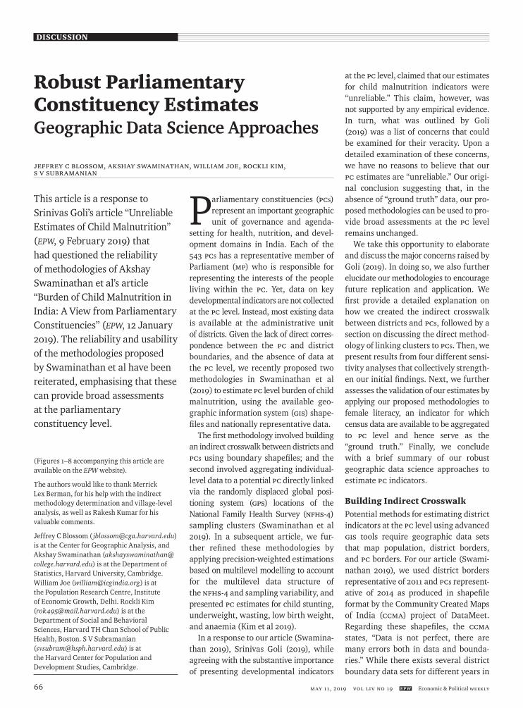
GIS format, this was the only source that had PC boundaries. Knowing we were going to intersect the two shapefi les, we wanted districts and PCs that were as closely matched as possible where the boundaries were coincident. The CCMA’s statement that “the external boundary of the district shapefi le produced by this project was derived from the PC bounda-ries” (DataMeet) indicated there was an effort made to match at least the periph-eral boundaries of districts and PCs. Vis-ual inspection of the district and PC shapefi les in GIS software confi rmed that a majority of the boundaries are in-deed coincident where they should be, with a few exceptions.

Figure 1 shows an area in Karnataka state where three district boundaries intersect. Notice the district and PC bor-ders between Vijayapura (Bijapur) and Yadgir and Vijayapura and Kalaburagi (Gulbarga) are perfectly coincident. However, the border between Kalabura-gi and Yadgir exhibits disparate district/PC boundaries, when in reality these probably should be coincident. How this data limitation affects the reliability of our estimates will be discussed after elaborating on the population data we chose to use.

Many population data sets exist for India in GIS format. For our analysis we wanted to model population ground conditions to most closely match the time period January 2015 to December 2016—the same year the NFHS-4 child malnutrition data were collected. We also desired a population data set with a fi ne enough spatial resolution to most closely repre-sent the disparate nature of the PC and district boundaries. In choosing an appropriate population data set for our study, we analysed the strengths and limitations of three different data sets, presented below.

LandScan global population database 2016: It is a population estimate pro-duced by the Oak Ridge National Labo-ratory using demographic census data and remote sensing imagery analysis in a dasymetric modelling approach. The model is tailored to match the data con-ditions and geographical nature of indi-vidual countries. LandScan represents

estimations of people per grid square in a raster data format at an approximately 1 kilometre (km) spatial resolution. This resolution varies from 960 metre (m) east to west by 960 m as measured in the extreme southern portion of Tamil Nadu province to 760 x 930 as measured in the extreme north of Jammu and Kashmir (J&K). Strengths of the LandScan population data are its complete cover-age across India and temporal represen-tation of the year 2016, which is within the time period of the NFHS-4. Limitations are that it presents population estimates, and not actual values, and at a spatial resolution of 900 m, it is in some locations too coarse to effectively model detailed variations exhibited by the PC boundaries.

AsiaPop 2015: It is a population estimate produced by the School of Geography and Environmental Science, University of Southampton, using demographic Census data, land cover remote sensing imagery analysis and a dasymetric modelling design. The model is adjusted to match the geographical conditions for individ-ual countries in Asia for 2015 (Gaughan et al 2013). AsiaPop 2015 represents esti-mations of people per grid square in a raster data format at an approximately 100 m spatial resolution. This resolution varies from 96 m east to west by 96 m as measured in the extreme southern por-tion of Tamil Nadu province to 75 x 90 as measured in the extreme north of J&K. Strengths of the AsiaPop 2015 popula-tion data are its complete coverage across India and temporal representation of 2015, which is within the time period of the NFHS-4, and its spatial resolution of 90 m is granular enough to effectively model districts and PCs that exhibit a heterogeneous mix of both rural and urban areas. Limitations are that it presents population estimates, not actual values.

Census of India 2011 village points: It represents population counts for 6,37,848 inhabitant villages from the 2011 Census of India. Villages were located by ML Infomap, a geospatial mapping company based in New Delhi, by digitising village locations as vector points using GIS. Sources for the village mapping were from the Indian Revenue Village

Boundary maps and small-scale Census Atlas maps. Locations are verifi ed using high resolution satellite imagery. Using the Village Census Code, the 2011 Census data was linked to the village locations.1 Strengths of using this data for popula-tion modelling are that it has complete coverage for all of India, it is a true pop-ulation count, and also includes popula-tion of children less than six years old. Limitations are that the population values are linked to discrete point locations at the centre of villages and they are from 2011, which is four–fi ve years before the NFHS-4 data was collected.

Census of India 2011 village polygons: It also represents actual population counts for villages from the 2011 Census of India. Village boundaries were located by ML Infomap, by digitising village polygon boundaries (where available) from Indian Revenue Village Boundary maps and small scale Census Atlas maps. Locations were verifi ed using high resolution satel-lite imagery.2 Using the Village Census Code, the 2011 Census data was linked to the village locations. This data set does not include village polygons for the states of Nagaland, Mizoram, Meghalaya, Manipur, Arunachal Pradesh, and An-daman and Nicobar Islands. Strengths of using this data for population modelling are that it is a true population count and includes population of children less than six years old. Limitations of using this data are that the population values are linked to discrete point locations at the centre of villages, that they are from 2011, and not all of India is represented.

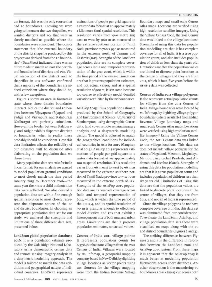
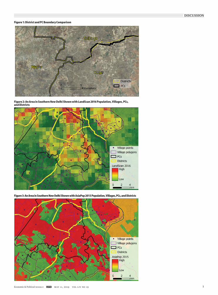
Since the village polygons do not have complete coverage of India, this data set was eliminated from our consideration. To evaluate the LandScan, AsiaPop, and village population data sets these were visualised on maps along with the PC and district boundaries (Figures 2 and 3).

The striking difference between Fig-ures 2 and 3 is the difference in resolu-tion between the LandScan 2016 and AsiaPop 2015 rasters. From these maps it is apparent that the AsiaPop 2015 is much better at modelling population fl uctuations across short distances. An-other observation is the meandering PC boundaries (black lines) cut across both

DISCUSSION


districts and villages. This evaluation led us to eliminate the LandScan popula-tion raster from consideration due to its coarse resolution. Village point locations were eliminated due to their discrete locational nature, representing all village population at one centroid point. This presents a problem where PCs cross through villages, causing all of the vil-lage population to be assigned to the PC in which the point is located, and zero village population being assigned to the remaining PCs the village overlaps with.

Therefore, we concluded that due to its high resolution that effectively models the heterogeneous nature of areas tran-sitioning from urban to rural and its complete coverage of India and temporal harmony with the NFHS-4 data, the Asia-Pop 2015 would be the most appropriate population data set to use for our analysis. The AsiaPop 2015 is also widely used for other geospatial analyses.

In order to facilitate replication of our methodology, we further elaborate on the subsequent workfl ow involved in creating the indirect crosswalk to produce the PC-level malnutrition estimates:

We also take this opportunity to correct the mischaracterisations made by Goli (2019) on our indirect crosswalk meth-odology. Specifi cally, contrary to Goli’s reading that the PC_District_Intersect

implicitly assumes homogeneity within a district, our methodology does not assume a homogeneous population within dis-tricts. The GIS Intersect command actu-ally splits the geometry of the PCs and districts, creating new areas that are pieces of districts. Applying the popula-tion zonal statistics to each of these pieces accounts for the mix of urban and rural population distribution within districts. We also calculated areal percentages for the intersected data, chiefl y for two rea-sons: (i) to identify and eliminate “sliver” polygons generated by slight boundary inaccuracies between the district and PC shapefi les; and (ii) by calculating percent area; this allows for additional, non-human data at the district level to be analysed at the PC level. For example, total forest or wetland or other natural features tabulated at the district level can be apportioned to the PC level using the area percentages.

Direct Methodology

The second method we had proposed in our original article (Swaminathan 2019) involved aggregating individual-level data

to a potential PC linked via randomly displaced GPS locations of the NFHS-4 sampling clusters. We requested and downloaded the GPS cluster locations from the Demographic Health Surveys

(DHS 2016) Programme for India. The cluster locations in this data fi le con-tained a “LATNUM” fi eld listing the clus-ter’s latitude coordinate in decimal de-grees and a “LONGNUM” fi eld which lists the cluster’s longitude coordinate in decimal degrees. Using the ArcGIS AddXY command, these cluster loca-tions were converted into a shapefi le for use in GIS. In order to ensure respondent confi dentiality, the DHS/NFHS randomly displaced the GPS latitude/longitude positions such that urban clusters were displaced up to 2 km and rural clusters were displaced up to 5 km, with 1% of the rural clusters displaced up to 10 km.

The displacement was restricted so that the points stay within the same district. This gave us the confi dence to overlay district boundaries with each cluster to determine its district. Specifi -cally, we performed an ArcGIS Spatial Join from each cluster location to the districts shapefi le. This GIS command does a “point in polygon” test, and cal-culates the district each cluster falls in, saving this information into a new col-umn of the cluster attribute table. We then performed an ArcGIS Spatial Join between the cluster shapefi le and the PC boundaries. This determined which PC each cluster fell into. After determining the PC that each cluster fell into, we summarised the cluster populations to create a “sample population” for each PC. Prevalence for the malnutrition indicators was then computed, that is, number of individuals with each condition divided by the total number of individuals in the PC.

We recognise that this methodology may misclassify some clusters to fall into incorrect PCs due to the random

1 The ArcGIS Intersect command was applied to the district and PC shapefiles, creating a new shapefile where each new polygon contained both the district ID and PC ID of the overlapping area.

2 Area was calculated for the new polygons using the Kalianpur 1975/India Zone IIa (EPSG:24379) coordinate system.

3 New areas were compared to the original district areas by dividing the new area by the total district area. Polygons with less than a hundredth of a percent of the original district area were deleted. These extremely small areas are “slivers” that act as noise, and are created from slight boundary inaccuracies between the district and PC shapefiles The ArcGIS Intersect command was applied to the district and PC shapefiles, creating a new shapefile where each new polygon contained both the district ID and PC ID of the overlapping area.

4 The percentage population for the intersected areas was calculated by performing an ArcGIS Zonal Statistics overlay with the intersected shapefile and the AsiaPop 2015 population raster to produce a total population per intersected polygon.

5 To determine the percentage of district population in each intersected polygon, the new population was divided by the total population of the district.

6 The district segments were matched to the NFHS-4 district level data using an ArcGIS Table Join based on the district ID.

7 Each district-level malnutrition percentage was multiplied by the total district population, to produce an estimated number of individuals in each district with a particular malnutrition state.

8 The number of individuals in each district with a particular malnutrition state was multiplied by the percentage of the district population contained in each intersected segment, producing an estimate of individuals in each district segment with a particular malnutrition state.

9 The intersected shapefile was summarised by PC ID, producing total individuals in each PC segment with a particular malnutrition state, and total population in each PC.

10 The total individuals in each PC with a particular malnutrition state was divided by the total population in each PC to produce estimates of percentage population with a particular malnutrition state for each PC.

EPW Index

An author-title index for EPW has been prepared for the years from 1968 to 2012. The PDFs of the Index have been uploaded, year-wise, on the EPW website. Visitors can download the Index for all the years from the site. (The Index for a few years is yet to be prepared and will be uploaded when ready.)

EPW would like to acknowledge the help of the staff of the library of the Indira Gandhi Institute for Development Research, Mumbai, in preparing the index under a project supported by the RD Tata Trust.

DISCUSSION


displacement of GPS coordinates. Figures 4 and 5 illustrate possible cluster/PC mis-classifi cations. In Figure 4, the southern-most rural cluster point (red dots) on this map is at risk of misidentifi cation due to inaccurate PC boundary. It falls in a Firo-zabad PC, but visual inspection of the lo-cation compared to the satellite imagery reveals it should be in Agra. In Figure 5, rural cluster point in Rajgarh PC is 0.4 km from the PC border with Guna, risking classifi cation in the wrong PC.

Yet, the resulting measurement error will most likely be random when aggre-gated. Given the highly consistent PC estimates for child malnutrition indica-tors when comparing the indirect cross-walk and direct methodologies (r = 0.92 for stunting, r = 0.92 for underweight, r = 0.84 for wasting, and r = 0.89 for anaemia) (Swaminathan 2019), as well as the relative simplicity of the direct methodology, we encourage the latter approach when GPS coordinates for sur-vey clusters are available to be linked to PC boundaries.

Sensitivity Analyses

Prompted by other issues raised by Goli (2019), we conducted the following sen-sitivity analyses and can conclusivelly say that our original fi ndings remain robust. First, we identify PCs that share the same boundary as the districts and compare the estimated child malnutrition prevalences for PCs to the values given in the NFHS-4 district reports. Second, we use child population (0–6 years) instead of total population for the indirect crosswalk and re-estimate the PC level malnutri-tion indicators. Third, we apply sam-pling weights at the district level. Fourth, we summarise fi ndings from our recent study (Kim et al 2019) where we incorporated precision-weighting to ac-count for small samples. For brevity, we conduct these sensitivity analyses for stunting only. We also note that ranking and prevalence of all child malnutrition indicators for all PCs are available upon request to the authors as noted in the corrected Appendix of our original pub-lication, that is, Swaminathan (2019).

PCs and districts with ‘matching’ boundaries: One way to test the validity

of our model is to analyse our malnutri-tion estimates in PCs that exhibit identi-cal boundaries with a district. To fi nd these exact matches, we compared the total area of each PC with the total area of each intersecting district. There were no PC/district combinations that exhib-ited a zero percent difference in area, due to the boundary inaccuracies de-scribed above. Knowing that in reality there are many PCs and districts that are identical, we visually inspected all PC/district area comparisons that exhibited less than a 4.0% difference in area. This revealed 28 PCs that were identical with a district boundary. In an ideal scenario, our estimated child malnutrition preva-lence rates in these PCs should perfectly match the district-level NFHS-4 data, and indeed this is what we found (Table 1).

For stunting, the correlation between PC estimates and NFHS-4 district estimates was r = 0.982 for indirect crosswalk estimates and r = 0.995 for direct

estimates. The difference in stunting prevalence between PC estimates and the NFHS-4 district estimates was less than 1.0% for 20 out of 28 PCs/districts, with the largest difference being 7.4% for Maharajganj using indirect crosswalk estimates and 2.7% for Krishnagiri using direct estimates.

Using child population for indirect crosswalk: In our original article, the population calculations involved in the indirect crosswalk methodology repre-sented all age groups. We had intentionally used the total population to encourage our apportioning method to be applied to other various health and development indicators that affect the general popu-lation. However, given that malnutrition indicators we had investigated are

relevant for population of children only, we performed a sensitivity analysis to generate PC estimates for stunting using the 0–6 year old population from the 2011 Census. Of note, children surveyed in NFHS-4 were under fi ve, and hence do not per-fectly match with the child population defi ned in the census. Moreo-ver, our model does not account for the differ-ences in age distribution among the neighbour-ing districts. Neverthe-less, the resulting stunt-ing estimates from this sensitivity analysis re-mained identical to the estimates we had gen-erated using the total population (r = 0.98) (Figure 6).

Applying sampling wei-ghts: The use of sam-pling weights made mini-mal difference at the

district level, and hence our PC esti-mates generated from unweighted dis-trict level data are unlikely to be affected. For instance, the correlation in weighted

Table 1: Comparing PC Stunting Estimates Derived from Indirect Cross-walk and Direct Methodologies to the District Stunting Estimates from NFHS-4 (across 28 PCs/districts with identical boundaries) PC/District with State PC Stunting PC Stunting DistrictIdentical Boundaries %, Indirect %, Direct Stunting %, Estimates Estimates NFHS Report

Araria Bihar 48.4 48.6 48.4

Gopalganj Bihar 35.6 36.8 35.6

Begusarai Bihar 44.9 45.0 44.9

Arrah (Bhojpur) Bihar 43.5 43.9 43.5

Nalanda Bihar 54.1 54.4 54.1

Surguja Chhattisgarh 37.3 32.3 32.3

Jamnagar Gujarat 27.9 29.7 27.9

SabarKantha Gujarat 50.6 51.5 50.6

Anand Gujarat 45.3 46.9 48.2

Jamshedpur (Purbi Singhbhum) Jharkhand 39.3 41.0 39.3

Vijayapura Karnataka 44.9 44.8 44.9

Davangere Karnataka 46.4 48.3 46.4

Chhindwara Madhya Pradesh 33.6 33.5 33.6

Jajpur Odisha 30.3 29.8 30.3

Sundargarh Odisha 37.2 36.6 37.2

Jalandhar Punjab 28.2 29.6 29.3

Kanyakumari Tamil Nadu 17.2 18.2 17.2

Krishnagiri Tamil Nadu 24.7 22.4 25.1

Thoothukudi Tamil Nadu 21.2 21.1 21.2

Rampur Uttar Pradesh 46.0 45.2 46.0

Shahjahanpur Uttar Pradesh 49.3 49.4 49.3

Mathura Uttar Pradesh 42.1 40.3 40.8

Domriaganj (Siddarth Nagar) Uttar Pradesh 54.3 56.4 57.9

Firozabad Uttar Pradesh 46.0 44.2 44.0

Maharajganj Uttar Pradesh 45.9 54.6 53.3

Mirzapur Uttar Pradesh 49.1 48.5 49.1

Fatehpur Uttar Pradesh 52.4 52.5 52.4

Unnao Uttar Pradesh 44.7 46.9 46.5

DISCUSSION


versus unweighted district estimates was above 0.99 for stunting (Figure 7).

Precision-weighting: In our more recent work (Kim et al 2019), we used multilevel models to generate PC estimates based on precision-wei ghted predicted probabili-ties of child undernutrition indicators at the cluster level (that is, villages in rural areas and census enumeration blocks in urban areas). This methodology is well known to provide a technically robust and effi cient framework to generate small area estimations by accounting for sampling variability (Goldstein 2011; Jones and Bullen 1994). In our compre-hensive assessment of PC estimates using different statistical modelling (precision-weighted versus none) and methodolo-gies to identify PC membership (direct versus indirect crosswalk), we found very high consistency with r = 0.92–0.99 for stunting (Kim et al 2019).

Validation of Methodologies

A formal validation of our PC estimates for child malnutrition indicators neces-sitates census data on anthropometry and haemoglobin measures of all chil-dren in India linked to PC identifi ers. In the absence of such data, we sought to validate our methodologies by applying them to a key developmental indicator, and a strong predictor of child malnutri-tion, for which census data are availa-ble. We have a sense of “ground truth” on the extent of female literacy, which can be aggregated to the PC level, from the 2011 Census. The NFHS-4 also col-lected information on literacy for all sur-veyed women, enabling us to generate PC estimates by using the proposed indirect crosswalk and direct linkage methodologies. Comparison of our esti-mates to the PC-level proportion of liter-ate females from the census indicated an incredibly high correlation of r = 0.96–0.97 for both indirect crosswalk and direct methodology (Figure 8). Although there are some differences between the census data and NFHS-4 survey in terms of population coverage (all females older than six years in the census versus 15–49 year olds surveyed in NFHS-4) and time of data collection (2011 for census versus 2015–16 for NFHS-4), this exercise clearly

demonstrates the validity of our pro-posed methodologies to generate PC level data.

In Conclusion

The analyses presented here further support that the two methodologies proposed in our earlier articles (Kim et al 2019; Swaminathan 2019) provide a robust assessment of child malnutrition at the PC level. It is well-recognised that monitoring data on population health and well-being at the PC level is impor-tant to increase political accountability and to effectively design and evaluate policies and programmes. In the absence of identifi ers for PCs in the current sur-veys and census data, we present two realistic methodologies using GIS that produce robust PC-level estimates given the currently available data in India. We have further elaborated on the two methodologies to aid application of our work on other diverse indicators of population health and development. We are optimistic that this increased awareness of PC-level data will lead to better policy decisions and overall leadership among PCs in India.

notes

1 Based on written correspondence of Jeffrey C Blossom with ML InfoMap.

2 Based on written correspondence by Blossom with ML InfoMap.

REFERENCES

DHS (2016): “India: Standard DHS, 2015–16,” DHS Program: Demographic and Health Surveys, https://www.dhsprogram.com/data/dataset/India_Standard-DHS_2015.cfm.

Gaughan, A E, F R Stevens, C Linard, P Jia and A J Tatem (2013): “High Resolution Population Distribution Maps for Southeast Asia in 2010 and 2015,” PLoS One, Vol 8, No 2, e55882, doi:10.1371/journal.pone.0055882.

Goldstein, H (2011): Multilevel Statistical Models, United Kingdom: Wiley.

Goli, S (2019): “Unreliable Estimates of Child Malnutrition,” Economic & Political Weekly, Vol 54, No 6, pp 64–67.

Jones, K and N Bullen (1994): “Contextual Models of Urban House Prices: A Comparison of Fixed-and Random-Coeffi cient Models Developed by Expansion,” Economic Geography, Vol 70, No 3, pp 252–72.

Kim, R, A Swaminathan, R Kumar, Y Xu, J C Blos-som, R Venkataramanan, A Kumar, W Joe and S V Subramanian (2019): “Estimating the Burden of Child Malnutrition across Parliamen-tary Constituencies in India: A Methodological Comparison,” SSM-Population Health, Vol 7, No 100375, doi:10.1016/j.ssmph.2019.100375.

Swaminathan A, R Kim, Y Xu, J C Blossom, J William, R Venkataramanan, A Kumar and S V Subramanian (2019): “The Burden of Child Malnutrition in India: A View from Parliamentary Constituencies,” Economic & Political Weekly, Vol 54, No 2, pp 44–52.

Review of Urban AffairsDecember 15, 2018

From Intermittent to Continuous Water Supply: —Isha Ray, Narayan Billava, A Household-level Evaluation of Water System Zachary Burt, John M ColforD jr, Reforms in Hubli–Dharwad Ayşe Ercümen, K P Jayaramu, Emily Kumpel, Nayanatara Nayak, Kara Nelson, Cleo Woelfle-Erskine

Sensitivity of Traffic Demand to Fare Rationalisation: —Sunil Ashra, Sharat Sharma, The Case of Delhi’s Airport Metro Express Link Narain Gupta

Roads to New Urban Futures: Flexible Territorialisation in Peri-urban Kolkata and Hyderabad —Sudeshna Mitra

Negotiating Street Space Differently: Muslim Youth and Alternative Learning —Rafia Kazim

Predicting the Future of Census Towns —Shamindra Nath Roy, Kanhu Charan Pradhan

Mission Impossible: Defining Indian Smart Cities —Sama Khan, Persis Taraporevala, Marie-Hélène Zérah

Recent Perspectives on Urbanisation: Ahmedabad Stories —Howard Spodek

For copies write to: Circulation Manager,

Economic & Political Weekly,320–322, A to Z Industrial Estate, Ganpatrao Kadam Marg, Lower Parel, Mumbai 400 013.

email: [email protected]

DISCUSSION


Figure 1: District and PC Boundary Comparison

Figure 2: An Area in Southern New Delhi Shown with LandScan 2016 Population, Villages, PCs, and Districts

Figure 3: An Area in Southern New Delhi Shown with AsiaPop 2015 Population, Villages, PCs, and Districts

DISCUSSION


Figure 4: Exemplification of Potential Misclassification of a Cluster and PC Using Direct Methodology (Case 1)

Figure 5: Exemplification of Potential Misclassification of a Cluster and PC Using Direct Methodology (Case 2)

Figure 7: District Estima tes for Stunting before and after Applying the Sampling Weights

0 10 20 30 40 50 60 70

Dis

tric

t est

imat

es fo

r stu

nti

ng

wit

hou

t sa

mp

ling

wei

gh

ts (%

)

70

60

50

40

30

20

10

0

District estimates for stunting with sampling weights (%)

r = 0.995

Figure 6: Correlation between Indirect Crosswalk Estimates Stunting Using Child Population (<6 Years) and Total Population

0 10 20 30 40 50 60 70

Ind

irec

t cro

ssw

alk

of P

C es

tim

ates

for s

tun

tin

g u

sin

g to

tal p

opu

lati

on (%

)

70

60

50

40

30

20

10

0

Indirect crosswalk of PC estimates for stunting using population <6 years old (%)

r = 0.98

Figure 8b: Validation Test Comparing PC Female Literacy from Census 2011 to Direct Methodology

30 40 50 60 70 80 90 100

Dir

ect m

eth

od

olo

gy

of P

C es

tim

ates

for

fem

ale

liter

acy

(%)

100

90

80

70

60

50

40

30

PC female literacy from 2011 Census (%)

r = 0.96

Figure 8a: Validation Test Comparing PC Female Literacy from Census 2011 to Indirect Crosswalk Estimates

30 40 50 60 70 80 90 100

Ind

irec

t cro

ssw

alk

of P

C es

tim

ates

for

fem

ale

liter

acy

(%)

100

90

80

70

60

50

40

30

PC female literacy from 2011 Census (%)

r = 0.97

robust parliamentary constituency estimates

Documents