OPTIMAL CONTROL APPLICATIONS & METHODS, VOL. 10, 255-266 (1989)

ROBUST PARAMETER ESTIMATION FOR FUEL COST MODELS IN ECONOMIC OPERATION OF ELECTRIC

POWER SYSTEMS

DARWISH M. K . AL GOBAISI Water & Electricity Department, P.O. Box 2623, A bu Dhabi, United Arab Emirates

A. C . BAJPAI Loughborough University of Technology, Loughborough, Leicestershire, U.K.

AND

P. N . P . SINGH Water & Electricity Department, Abu Dhabi, United Arab Emirates

SUMMARY

This paper is focused on optimal parameter estimation of fuel cost models intended for economic scheduling of electric power systems. The common approaches of least squares and conventional weighted least squares may not be appropriate for situations involving non-normally distributed measurement errors. Techniques of robust parameter estimation, in particular the iteratively reweighted least-squares estimator, offer an attractive option in these situations.

The paper discusses the theoretical aspects of this powerful technique and presents computational experience with a number of popular choices of weighting functions. A comparative evaluation of the parameter estimates obtained is carried out in terms of both accuracy of the estimates and their effects on economic scheduling strategies. K E Y WORDS Robust parameter estimation Fuel cost models Electric power systems

Iteratively reweighted least-squares estimators Economic power scheduling strategies

INTRODUCTION

Research in the area of modelling unit and system performance for economy-security functions in electric power systems is directed at obtaining better model parameters for the potential savings and improved security. The area of parameter estimation for economic scheduling of power systems has received some attention recently. El-Hawary and Mansour’ present formulations and computational results for a number of models used in economic scheduling of electric power systems. Their approach is a weighted least-squares estimation process, and performance comparisons with Gauss-Newton, Powells’ regression and Marquardt’s regression are given. Conclusions have been drawn from a study of a number of data sets’ dealing with common thermal generation unit types and their performance.

The importance of accurate parameters in economic scheduling has been recognized for many years, and sensitivity analysis studies by R i r ~ g l e e , ~ Dillon and Tun4 and Vemuri and Hill’ point out the potential loss in economy resulting from the use of inaccurate parameters. As a

0 143-2087/89/030255- 12$06.00 0 1989 by John Wiley & Sons, Ltd.

Received 5 October 1987 Revised 27 October 1988

256 D. M . K . AL GOBAISI. A. C. BAJPAI AND P. N. P. SlNGH

motivation to accurate modelling in economic scheduling studies, El-Hawary and Christensen6 give an account of loss in economy resulting from erroneous modelling assumptions.

I t must be emphasized that previous work on parameter estimation for fuel cost models has been based on the application of the least-squares approach and its variants such as recursive estimation and weighted least-squares estimation. ' The literature on regression analysis' indicates that these estimators may not be appropriate for data involving measurement error distributions that are not normal. In this case, robust regression techniques specifically designed to suppress the influence of bad data (outliers) are often recommended.

As part of a larger study involving the economic dispatch of a 1500MW, 56-unit, predominantly thermal electric power system, an investigation into model parameter estimation techniques appropriate for the system was conducted. Initially, conventional techniques were employed and a fully integrated dispatching algorithm suite was implemented. We then decided to explore the application of robust parameter estimation techniques to a selected set of units in the system. These units are characterized by being the ones that follow the system demands closely. The aim of the study was to identify possible erroneous data (represented by outliers) and to use the newly acquired parameter estimates in the actual dispatching of the system.

In this paper, the theoretical aspects of robust estimators, in particular the iteratively reweighted least-squares approach, are detailed. Cornputational results pertaining to five data sets representing more than 12 units in the 56-unit system are given. A comparison of economic dispatch results obtained using alternate parameters and those obtained using conventional least squares is given.

FUEL COST PARAMETER ESTIMATION

A common practice in economic dispatch studies is to assume that the input-output curve for a thermal generating unit is represented by a second-order polynomial in the active power generation P(in MW):

(1)

where F is the hourly fuel input (Mcal hr-I) . The parameter estimation problem is one of finding the parameters UO, al and a2 given n

measurements relating the fuel cost F( i ) to the ith power generation P ( i ) . Usually n is greater than the number of parameters to be estimated (three in the present application). One thus writes the measurement model as

F ( P ) = a0 + alp + azPZ

F ( i ) = [ I P ( i ) ~ ' ( i ) ] a1 + u ( i ) i = I , ..., n (2) [::I where u( i ) is the measurement noise sequence. In the parameter estimation terminology we write

(3) z ( i ) = hT( i )X + v ( i )

where

z ( i ) = F ( i ) h T ( i ) = [ 1 P ( i ) P 2 ( i ) ]

PARAMETER ESTIMATION FOR ECONOMIC POWER SCHEDULING 257

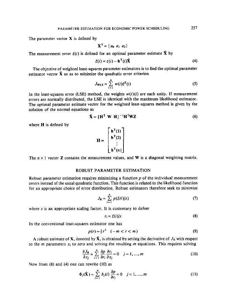
The parameter vector X is defined by

X T = [a0 a1 a21

5(i) = z ( i ) - hT( i )2

The measurement error 5(i) is defined for an optimal parameter estimate ?t by

(4)

The objective of weighted least-squares parameter estimators is to find the optimal parameter estimator vector 2 so as to minimize the quadratic error criterion

In the least-squares error (LSE) method, the weights w ( t ) ( i ) are each unity. If measurement errors are normally distributed, the LSE is identical with the maximum likelihood estimator. The optimal parameter estimate vector for the weighted least-squares method is given by the solution of the normal equations as

(6) 2 = [ H T W HI -'HTWZ

where H is defined by

The n x 1 vector Z contains the measurement values, and W is a diagonal weighting matrix.

ROBUST PARAMETER ESTIMATION

Robust parameter estimation requires minimizing a function p of the individual measurement errors instead of the usual quadratic function. This function is related to the likelihood function for an appropriate choice of error distribution. Robust estimators therefore seek to minimize

n

JR = c p ( W ) / s ) I = I

where s is an appropriate scaling factor. It is customary to define

r; = .f(i)/s

In the conventional least-squares estimator one has

p ( r ) = t r2 ( - 00 < r < 00 ) (9) A robust estimate of X, denoted by 2, is obtained by setting the derivative of J R with respect

to the m parameters X j to zero and solving the resulting m equations. This requires solving

Now from (8) and (4) one can rewrite (10) as

258 D. M . K . AL GOBAISI, A . C. BAJPAI AND P. N. P . SINGH

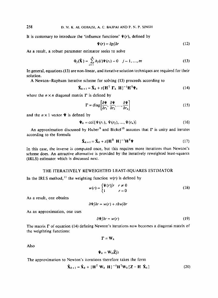
It is customary to introduce the 'influence functions' q ( r ) , defined by

+ ( r ) = ap/ar

As a result, a robust parameter estimator seeks to solve

+ j ( i ) = i h j ( i ) q ( r i ) = o j = 1, ..., m i = 1

In general, equations (13) are non-linear, and iterative solution techniques are required for their solution.

A Newton-Raphson iterative scheme for solving (13) proceeds according to

X k + l = & + S [ H T r k H ] - ' H T * k (14)

where the n x n diagonal matrix r is defined by

and the n x 1 vector + is defined by

* k = coI[q(rO, \k(r2), ..., *(r,,)l

An approximation discussed by Huber9 and Bickel" assumes that r is unity and iterates

(17)

In this case, the inverse is computed once, but this requires more iterations than Newton's scheme does. An attractive alternative is provided by the iteratively reweighted least-squares (IRLS) estimator which is discussed next.

according to the formula R k + I = X k + S [ H T HI - 'HT*

THE ITERATIVELY REWEIGHTED LEAST-SQUARES ESTIMATOR

In the IRLS method, the weighting function w(r) is defined by

q ( r ) / r r z 0 [l r=O

w(r) =

As a result, one obtains a\k/ar = w(r) + rdw/dr

aq/ar = w(r)

As an approximation, one uses

The matrix r of equation (14) defining Newton's iterations now becomes a diagonal matrix of the weigthting functions:

r=wk Also

* k = W k z / S

The approximation to Newton's iterations therefore takes the form

& + I = & + [ H T W k H ] - ' H T W k [ Z - H x k ]

PARAMETER ESTIMATION FOR ECONOMIC POWER SCHEDULING 259

The IRLS method only requires knowing how to compute the weight functions w ( r ) . Then it is possible to use an existing weighted least-squares algorithm to obtain updates of %. A fundamental issue in IRLS estimation is that of choosing the weight functions w ( r ) .

A number of robust criterion functions have been proposed. These robust estimation procedures can be classified according to the behaviour of their influence function *. The latter controls the weight given to each measurement error. After some years of experience with robust estimation, Holland and Welsch l 1 chose eight weight functions. These are designed not to weight large measurement errors as heavily as the least-squares method does. Holland and Welsch give nominal values for tuning constants associated with each function to guide in the selection process. The IRLS method is implemented in ROSEPACK. l2 The weighting functions are defined as follows.

The Andrews weighting function

This function is classified as a hard descender13 and is defined by

sin(r/A) 1 r I < nA Irl > nA

w ( r ) =

The recommended value

The biweight function

of the tuning constant A is 1 *339.

This is attributed to Beaton and Tucky l4 and is classified as a hard descender. The nominal value of the tuning constant B is 4.685. The function is defined by

The Cauchy weight function

This is referred to as the t-likelihood function and is a soft redescender defined by

w ( r ) = [ I +(r/c)*]-l

where the nominal value of C is 2.385.

The Fair weighting function

nominal tuning constant F of 1.400, the Fair function is defined as This function is designed to approximate the least absolute residuals estimator. I' With a

w ( r ) = ( 1 + I rl / F ) - '

The Huber weighting function

This is defined by t6

260 D. M. K . AL GOBAISI. A. C. BAJPAI AND P. N . P. SlNGH

The logistic function

This is defined by w(r) = (L/r)tanh(r/L)

where L = 1 .205.

The Talwar function

This function is defined by”

The nominal value of T is 2.795.

The Welsch weighting function

This soft redescender is defined by‘*

w(r) = exp[ - (r/w)’]

The nominal tuning constant W is 2.985.

The value of the starting estimate %O should be chosen carefully, since using the least-squares solution as an initial estimate can disguise high residual points. The least absolute residual estimate (LARE) is recommended as a good choice.

Robust estimation algorithms are extremely helpful in locating bad points (outliers) and highly influential measurements. Whenever a least-squares analysis is performed, it will be useful to perform a robust fit also. If the results of the two procedures are in substantial agreement, one should use the least-squares results, because conclusions based on least squares are at present better understood. However, if the results of the two analyses differ, the reasons for these differences should be identified. Measurements that are down-weighted in the robust fit should be carefully examined.

COMPUTATIONAL RESULTS

An extensive computational experiment to explore the application of the LARE and IRLS estimators to the system under consideration was conducted. On the basis of the system economic dispatch results, a number of units were selected for the study. Data for units 2-5, 28,42,44 and 45-50 of a 56-unit, all-thermal electric power system were considered, since these units experienced more changes in optimal loading than all other units did. In total, five data sets were examined out of a possible 30 data sets.

The object of the experiments was to ascertain the validity of the least-squares parameter estimates and the underlying assumption of a Gaussian error distribution. The results of the experiment were used to determine the most economic mode of loading based on the newly obtained parameters of the units considered. Comparisons and conclusions in terms of various error measures, loadings and minimum cost were also made in the work reported in this section.

The experiments were conducted using the Robust Statistical Estimation package (ROSEPACK) implementations of the LARE and IRLS estimators on a DEC Micro-VAX I1 in Fortran 77. The convergence criterion used was on the scaled errors in the parameter

PARAMETER ESTIMATION FOR ECONOMIC POWER SCHEDULING 26 1

estimates. Scaling of elements of the vector Z and the matrix H was carried out using column maximum element scaling. Least absolute residual estimates were used to initiate the iterations.

Experiments using the eight weighting functions and the LARE estimators were conducted. Elements of the diagonal weighting matrix were examined on each iteration. Recommended default values of the tuning constant for each weighting function were used. The following error measures were considered and are reported in this section:

SSR sum of the squares of the residuals (measurement errors) - this is the Lz-norm; SAR sum of the absolute values of the residuals-this is the LI-norm; MAXRE maximum of the absolute values of the residuals - this is the L,-norm.

The last measure is useful for ranking purposes using error measures. This is because LSE will always yield the lowest SSR, and LARE will result in the lowest SAR by their very definitions.

I t should be noted in the application of IRLS that whenever the scaled residual is less than the tuning constant of the weighting function, the value of the weighting will be unity for that measurement. If all scaled residuals are less than the tuning constant, the algorithm returns an estimate which is precisely that of the LSE.

The results and conclusions given in this section can be divided into two parts. In the first, conclusions using statistical measures from ROSEPACK are drawn, and in the second, results of economic dispatch from the GRG algorithm are used to further evaluate the conclusions from an end-use point of view. This latter part is a unique contribution of this investigation.

Data for the four identical units 2-5 are listed in Table I, and the results obtained using ROSEPACK are given in Table 11. Of the eight weighting functions, only the Andrews function results in estimates different from the LSE values. These are listed in Table I1 along with the error measures. Here, LSE and Andrews give almost identical parameters. MAXRE is lowest for the Andrews estimates.

Table 111 lists fuel cost measurement data for unit 28. These data are used to obtain the parameter estimates shown in Table IV. Note that for this unit, three weighting functions result in new estimates. These are the Andrews, Huber and Talwar weighting functions. The LSE

Table 1. Fuel cost measurement data for units 2-5

P(MW) 10 1 1 12 13 14 15 16 17 18 19 20 F(kca1 h - l ) 12.92 14-20 15.48 16.77 18.06 19.34 20.59 21.85 23-06 24.26 25.50

Table 11. Comparison of parameter estimates and error measures for units 2-5

a0 a1 a2 SSR SAR MAXRE

LSE -0.7356019 1.415329 -0.00518677 0.0025847 0.1393057 0.023969 LARE -0.7518344 1.416294 -0.00518509 0.002718609 0.131484 0.02740669 Andrews -0.7359567 1.415346 -0.00518617 0.002584885 0.138885 0.023883

Table I l l . Fuel cost measurement data for unit 28

P(MW) 20 25 30 35 40 45 50 55 60 65 70 75

F(kca1 h - ' ) 61.20 69.38 78.60 89.78 101.0 112.5 124.0 135.85 147.6 159.9 172.2 184-5

262 D. M . K . AL GOBAISI, A . C. BAJPAI A N D P. N. P. SINGH

Table IV. Comparison of parameter estimates and error measures for unit 28

Qo QI a2 SSR SAR MAXRE

LSE 23.48927 1.698061 0*006092007 5.027196 6.14531 1.3146 LARE 2 1 -01 563 1 a809463 0*005004488 6.262388 5.047783 1 -993324 Andrews 18.77898 1.883038 0.00439636 10.24764 5 -659702 3 ~001726 Huber 20.42926 1.832238 0.00477977 6.803525 5.262701 2.21407 Talwar 19.07516 1.871445 0.00450209 9.609438 5.645875 2-895098

Table V. Fuel cost measurement data for unit 42

P(MW) 6 7 8 9 10 1 1 12 13 14 15 16 F(kcal h - ' ) 12.00 16.24 18.46 20-66 22.82 24.99 27.18 29.54 31.93 34.43 37.04

values for uo and uz are the highest, and the value of al is the lowest. In terms of SSR, LARE and Huber are closest to the LSE measure, whereas Huber and Andrews are closest to LARE in terms of SAR. MAXRE is lowest for the LSE estimates.

Table V gives the data for unit 42, and the corresponding results of the parameter estimation are given in Table VI. For this unit, only the Andrews weightings result in parameter estimates different from the LSE parameters. The highest values of a0 and a2 are due to Andrews, which can also be seen to be a good compromise on SAR and SSR between LARE and LSE estimates.

Data for unit 44 are given in Table VII, and the corresponding parameter estimates and error measures are given in Table VIII. Here, note that the Andrews and Huber functions are active for this data set, and that the LSE estimates give the highest a0 and uz. The best (lowest) maximum residual is also due to LSE. The Andrews SSR is closest to the LSE value, and its SAR is closest to that of LARE.

The fifth data set is for units 45-50 and is listed in Table IX. The parameter estimation results are given in Table X. Note that the Andrews parameter estimates are close to those for the LSE estimator .

Table VI. Comparison of parameter estimates and error measures for unit 42

SAR MAXRE a0 Q l a2 ss R

LSE 2.504698 1.812307 0*02113061 0*1015925 0.9186739 0.1392401

LARE 2.587843 1.799369 0.0215628 0-1031212 0.8775129 0.1603174

Andrews 2.51777 1.810364 0.02119283 0.1016335 0.9121832 0.1429066

Table VII. Fuel cost measurement data for unit 44

P(MW) 6 7 8 9 10 I 1 12 13 14 I5 16

F(kcal h - ' ) 30-68 15.90 18.12 20.33 22.54 24.74 26.95 29-25 31.64 34.13 36.80

PARAMETER ESTIMATION FOR ECONOMIC POWER SCHEDULING 263

Table VIII. Comparison of parameter estimates and error measures for unit 44

a0 al a2 SSR SAR MAXRE ~ ~ ~ ~

LSE 2.025374 1.840458 0*02019813 0.09606672 0.9137835 0,1565771

LARE 1 m753449 1.900622 0.01718764 0.1081 151 0.8275089 0-236557

Andrews 1 e997309 1-847085 0.01984565 0.0963388 0.9003233 0.1688386

Huber 1-453874 1 a967021 0,01367429 0.1768975 0.9124443 0,3731728

Table IX. Fuel cost measurement data for units 45-50

P ( M W 5 6 7 8 9 10 I 1 12 13 14 15

F(kcal h-I) 37-00 39.60 41-30 44.80 47.70 50.50 52.80 56-40 59.80 64.40 69.00

Table X. Comparison of parameter estimates and error measures for units 45-50

a0 a1 a2 SSR SAR MAXRE

LSE 30.11814 0.875764 0.1121209 2.226672 4 * 5697 19 0.65 15026

LARE 27.80556 1.408331 0*08611126 3.078162 4.472225 0 - 9 16664 1

Andrews 30.10572 0.8775339 0.112077 2 * 2267598 4.565876 0.654669

Table XI. Ranking of methods in terms of maximum absolute error

2-5 28 42 44 45-50

LSE 2 1 1 1 1

LARE 3 2 3 3 3

Andrews 1 5 2 2 2

Talwar 4

Huber 3 4

It is important at this point to attempt to rank the parameter estimates using the various methods in terms of the statistical error measures. Earlier, it was stated that the SSR for LSE would be the lowest and that the value of SAR would be lowest for LARE. MAXRE would be a good criterion for ranking. Table XI gives such a ranking for the five data sets for five sets of parameter estimates. It is clear that the LSE values are superior, but those for Andrews are a close second. The same conclusions can be drawn from Table XII, which gives the ranking in terms of SSR. In terms of SAR, the Andrews estimates are a close second to those of LARE (Table XIII).

One does not have enough information to properly rank the Talwar and Huber weighting functions. Therefore we will proceed with further evaluation on the basis of the intended use of the acquired parameters in performing economic dispatch of the 56-unit system. Table XIV

264 D. M. K . AL GOBAISI, A. C. BAJPAI AND P . N . P. SlNGH

Table XII. Ranking of methods in terms of sum of squares of error

2-5 28 42 44 45-50

LSE 1 1 1 1 1

LARE 3 2 3 3 3

Andrews 2 4 2 2 2

Talwar 5

Huber 3 4

Table XIII. Ranking of methods in terms of sum of absolute error

2-5 28 42 44 45-50 ~~ ~~

LSE 3 5 3 4 3

LARE 1 1 1 1 1

Andrews 2 4 2 2 2

Talwar 3

Huber 2 3

Table XIV. Comparison of minimum cost of operation using different parameter estimates

LSE Talwar Huber Andrews LARE

700

800

900

lo00 I100

I200

1300

1400

36 089-7

39 336-2

42 817.0

46 380.0

50 092.0

53 995.6

59 560.0

64 219.6

36 063.97

39 372.47

42 807.67

46 384.50

50 097.05

53 990.18

59 554.95

64 213.93

36 074.03

39 382-53

42 812.72

46 386.62

50 095 * 26

53 986.25

59551*12*

64 210*10*

36 051-81

39 272.89

42 745.38

46 311.04

50 017.77

53 909.03

59 474*05*

64 133*03*

36 078.00

39 336.00

42 8 1 5 . 0 0

46 381 a 0 0

50 092.00

53 995.00

59 561 -00

64 219.00

lists the minimum cost of operation using the parameter estimates for power demand values ranging from 700 to 1400MW. The Andrews results appear to be superior, as can be seen from Table XV.

The experiments evaluating the performance of the parameter estimates were conducted using the GRG dispatch. Parameters based on LSE estimation were retained, and only those new ones for each method were changed in the runs reported.

Results comparing the optimal power generation of the 56 units for loads of between 700 and 1400MW were obtained. For the 700MW demand, the optimal generations are identical when using the LSE and Andrews parameters. Lower generations for units 27, 28, 31, 36, 44, 45 and

PARAMETER ESTIMATION FOR ECONOMIC POWER SCHEDULING 265

Table XV. Ranking of methods in terms of minimum cost of operation

LSE Talwar Huber Andrews LARE

700 5 2

800 3 4 9 0 0 5 2

lo00 2 4 1100 2 5 1200 5 3 1300 3 2

1400 5 3

3 1 4 5 1 2 4 1 3 5 1 3 4 1 3 2 1 4 I* 5* 4

2' 1* 4

45-50 are required by the Andrews parameters, whereas higher generations are required at units 32, 37-40 and 42 for the 800MW demand.

Comparing the minimum operating costs, one finds that the values predicted by the Andrews parameters are consistently lower than those obtained using the LSE values. This takes place even for 700, 1300 and 1400MW where the optimal generations are identical and logically one would expect the same actual fuel costs to be incurred. One can conclude that the results of the comparison should be treated with more caution. It is important to note that if one takes a l000MW demand to be the annual average demand for the utility system considered, then a rough calculation reveals that the annual loss in economy is in excess of 600 x l o 3 Mcal if a dispatch strategy based on the LSE parameters is used. The monetary value of this cost difference is of significant importance.

The percentage relative differences in the minimum operating costs for the power demands considered are calucated as:

700MW 0 . 1 per cent 800MW 0 .16 per cent 900MW 0.167 per cent

l000MW 0.148 per cent 1l00MW 0.148 per cent 1200MW 0 . I6 per cent 1300MW 0.1443 per cent 1400MW 0.1348 per cent

Although all the differences are below 0 . 2 per cent and may be neglected from a numerical analysis point of view, it is important to realize that this can mean significant loss in economy over a span of years. Possible explanations of the discrepancy at 700, 1300 and 1400MW are (1) effects of round-off in listing solutions and (2) the Andrews fit underestimates the cost values at very low and high loadings on the units modelled.

CONCLUSIONS

In this paper, robust parameter estimation techniques offering an attractive alternative to conventional least squares have been investigated. Emphasis was given to the iteratively reweighted least-squares technique and its eight associated weighting functions. An attractive

266 D. M. K. AL GOBAISI, A. C. BAJPAl AND P. N. P. SlNGH

feature of the techniques considered is the fact that they can serve as diagnostic tools to verify whether the measurement errors are Gaussian or not. The techniques offer a compromise between the least absolute residuals and the least-squares estimation criteria.

The results of the work reported here on the application to data for a number of thermal electric power generating units in the Abu Dhabi system revealed that the measurement errors are almost Gaussian. The Andrews weighting function resulted in the lowest maximum of the absolute residuals. The Andrews, Huber and Talwar weighting functions resulted in parameter estimates that were significantly different from those obtained using the least-squares approach.

When we compare the sum of the squares of the error for all weighting functions tested, the results from the least absolute error criterion and the Huber weighting function yield values closer to those obtained by ordinary least squares. On the other hand, comparing the sum of the absolute residuals, one finds that the Huber and Andrews weighting functions are closest to the results of the least absolute residuals criterion. The Huber function therefore appears to offer a good compromise between the least-squares and least absolute residuals estimation criteria in terms of fitting error statistics.

A comparison of the techniques in terms of the intended use of the parameters as an optimal dispatch strategy has also been conducted. In this case, the performance evaluation test ranked the Andrews weighting function as the one yielding the lowest optimal cost.

In conclusion, it appears that the Andrews estimates have a slight edge over the least-square estimates in term of measurement statistics and optimal dispatch results.

REFERENCES 1. El-Hawary, M. E. and S. Y. Mansour, ‘Performance evaluation of parameter estimation algorithms for economic

2. Power Technologies Inc., Synthetic electric utility systems for evaluating advanced technologies’, Electric Power

3. Ringlee, R. J., ‘Sensitivity methods for economic dispatch of hydroelectric plants’, IEEE Trans. Automatic

4. Dillon. T. S . and T. Tun, ‘Application of sensitivity methods to the problem of optimal control of hydro-thermal

5 . Vemuri, S . and E. F. Hill, ‘Sensitivity analysis of optimum operation of hydro-thermal plants’, fEEE Trans.

6. El-Hawary, M. E. and G . S. Christensen, Optimal Economic Operation of Electric Power Systems, Academic

7. Mendel, J. M., ‘Discrete Techniques of Parameter Estimation, The Equation Error Formulation’, Marcel Dekker,

8. Montgomery, D. C. and E. A. Peck, ‘Introduction to Linear Regression Analysis’, Wiley, New York, 1982. 9. Huber, P . J., ‘Robust methods of estimating regression coemcients’, Second Int . Summer School on Problems

operation of electric power systems’, fEEE Trans. Power Appar. Syst., PAS-101, 574-582 (1982).

Research Institute Report EM-285, February 1977.

Control, AC-10, 315-322 (1965).

power systems, Optim. control appl. methods, 2 , 117-143 (1981).

Power Appar. Syst., PAS-%, 688-696 (1977).

Press, New York, 1979.

New York, 1973.

of Model Choice and Regression Analysis, Rheinhardsbrum, G . D. R., November 1975. 10. Bickel, P. J., ‘One-step Huber estimates in the linear model’, J. Am. Statist. Assoc., 70, 428-434 (1975). 1 I . Holland, P. W. and R. E. Welsch, ‘Robust regression using iteratively reweighted least squares’, Commun. Sfatist.

12. Coleman, D., P. W. Holland, N. Kaden, V. Klema and S. C. Peters, ‘A system of subroutines for iteratively

13. Andrews, D., P. Bickel, F. Hampel, P. Huber, W. Roger and J . Tukey, ‘Robust Estimates of Location: Survey

14. Beaton, A. E. and J. W. Tukey, ‘The fitting of power series, meaning polynomials, illustrated on band-

15. Fair, R. C., ‘On the robust estimation of econometric models’, Ann. Econ. Social Meas., 3 , 667-78 (1974). 16. Huber. P. J., ‘Robust estimation of a location parameter’, Ann. Math. Statist., 35, 73-101 (1974). 17. Hinich, M. J . and P. P. Talwar, ‘A simple method for robust regression’, J. Am. Statist. Assoc., 70, 113-119

18. Dennis, J . E. and R. E. Welsch, ‘A technique for nonlinear least squares and robust regression’, Proc. American

Theory Methods, A6, 813-827 (1977).

reweighted least squares computation’, ACM Trans. Math. Software, 6, 327-336 (1980).

and Advances’, PrinceIon University Press, Princeton, NJ, 1972.

spectroscopic data’, Technometrics, 16, 147-85 (1974).

( 1975).

Statistical Association, Statistical Computing Section, Washington DC, 1976, pp. 83-87.