robust model for fatigue life estimation from monotonic

Robust Model for Fatigue Life Estimation from

Monotonic Properties Data for Steels

by

Derek Hartman

A thesis

presented to the University of Waterloo

in fulfilment of the

thesis requirement for the degree of

Master of Applied Science

in

Mechanical Engineering

Waterloo, Ontario, Canada, 2013

© Derek Hartman 2013

ii

Author’s Declaration

I hereby declare that I am the sole author of this thesis. This is a true copy of my thesis, including any

required final revisions, as accepted by my examiners.

I understand that my thesis may be made electronically available to the public.

iii

Abstract

Determining the fatigue properties (Manson-Coffin and Ramberg-Osgood parameters) for a steel

material requires time consuming and expensive testing. In the early stages of a design process, it is not

feasible to perform this testing, so estimates for the fatigue properties need to be made. To help solve

this problem numerous researchers have developed estimation methods to estimate the Manson-Coffin

parameters from monotonic properties data. Additionally, other researchers have compared the results

from these various estimation methods for large material classifications. However, a comprehensive

comparison of these estimation methods has not been made for steels in different heat treatment

states. More accurate results for the best estimation method and therefore the best estimates for the

Manson-Coffin parameters can be made with smaller classifications, which have more consistent

properties. In this research, best estimation methods are determined for six steel heat treatments.

In addition to looking at steel heat treatment classifications, the estimation of the Ramberg-Osgood

parameters is also examined through the compatibility conditions. The Ramberg-Osgood parameters are

required for a fatigue life assessment, and so they must also be estimated. Without them, the approach

of estimating the fatigue properties using the estimation methods would not be practically useful.

Finally, in the comparison of the estimation methods, an appropriate statistical comparison

methodology is utilized; multiple contrasts comparison. This methodology is implemented into the

comparison of the different estimation methods, by comparing the estimated lives and the experimental

lives as a regression so that the entire life range can be considered.

This comparison of the estimation methods results in the knowledge of the best estimation method for

each classification and an estimation of the potential error in life due to the use of these estimated

fatigue properties. This is of practical benefit for a design engineer, as the results of this research can be

used to estimate the fatigue properties in the early stages of the design and the potential error in the

life estimate can also be incorporated into this early fatigue analysis. An expert system is developed to

summarize all of the knowledge gained from this research to assist a design engineer.

The estimation methods can also be utilized to get estimates of the variability of the fatigue properties

given the variability of the monotonic properties data, since there is a functional relationship developed

between the two sets of material properties. This variability is necessary for a stochastic design process,

in order to obtain a more optimally designed component or structure. Specimens used for fatigue

testing are only taken from one set of material specimens, and so the variability between the different

heat lots of steel is not accounted for in the variability obtained from testing. In this research, the

estimation methods are used to calculate this additional variability between material heat lots for the

fatigue properties and this can be added to the variability from fatigue testing. This gives an estimate for

the total variability in fatigue properties (entire population) for all steel obtained from a manufacturer.

Overall the estimation methods have a number of practical applications within a fatigue design process.

Their use and implementation needs to be supplemented by the appropriate knowledge of their

limitations and for what classifications they give the best results. This research aims to provide this

knowledge and expands their use to account for variability in fatigue properties for stochastic analysis.

iv

Acknowledgements

They are a number of individuals who I would like to thank, who without their assistance, this research

would not be possible.

I would like to thank my supervisor, Dr. Gregory Glinka for the assistance, guidance, support and coffee

he provided in the pursuit of this research. It would be very difficult to find a better supervisor.

I would also like to thank Eric Johnson, Deere & Company, who is the primary contact with regards to

this research and who made a great deal of the data utilized in this research available. Without his

support and that of Deere & Company, this research would not have been possible. I would also like to

thank Brent Augustine and Robert Gaster who assisted in gathering some research data and any other

technicians and engineers from Deere & Company who were involved with any of the data collection.

Without all of this data from Deere & Company, this research would not be possible. Additionally,

thanks to some of the personnel at SSAB Muscatine, IA who made some additional data available.

Thank you to the National Science and Engineering Research Council and Ontario Graduate Scholarship

who provided financial assistance for this degree.

Finally, thanks to my colleagues Sergey Bogdanov and Pasi Lindroth who had ideas bounced off of them

during this research and who helped to make an excellent research group.

v

Dedication

To my beautiful Lauren who has been there to support me through this degree.

vi

Table of Contents Author’s Declaration ..................................................................................................................................... ii

Abstract ........................................................................................................................................................ iii

Acknowledgements ...................................................................................................................................... iv

Dedication ..................................................................................................................................................... v

List of Figures ................................................................................................................................................ x

List of Tables ............................................................................................................................................... xv

List of Abbreviations .................................................................................................................................. xvii

Nomenclature ........................................................................................................................................... xviii

1. Introduction .......................................................................................................................................... 1

1.1. Strain-Life Method ........................................................................................................................ 4

2. Heat Treatment Classifications of Steels .............................................................................................. 9

2.1. Steel Classifications ....................................................................................................................... 9

2.2. Steel Heat Treatments ................................................................................................................ 10

2.2.1. Ferrite-Pearlite Steel ........................................................................................................... 11

2.2.1. Austempered Steel .............................................................................................................. 11

2.2.2. Martensite – Lightly Tempered Steel .................................................................................. 12

2.2.3. Martensite – Tempered Steel ............................................................................................. 12

2.2.4. Incomplete Hardened Steel ................................................................................................ 12

2.2.5. Carburized Steel .................................................................................................................. 13

2.2.6. Micro-Alloyed Steel ............................................................................................................. 13

3. Literature Review ................................................................................................................................ 14

3.1. Introduction ................................................................................................................................ 14

3.2. Four-Point Correlation Method (FPM) by Manson [18] ............................................................. 15

3.3. Modified Four-Point Correlation Method (MFPM) by Ong [23] ................................................. 17

3.4. Universal Slopes Method (USM) by Manson [18] ....................................................................... 19

3.5. Modified Universal Slopes Method (MUSM) by Muralidharan and Manson [26] ...................... 20

3.6. Mitchell’s Method (MM) by Mitchell and Socie [28] .................................................................. 21

3.7. Modified Mitchell’s Method (MMM) by Park and Song [12]...................................................... 22

3.8. Medians Method (MedM) by Meggiolaro and Castro [21] ........................................................ 23

3.9. Method of Variable Slopes by Hatscher [29] .............................................................................. 24

vii

3.10. Uniform Material Law (UML) by Bäumel and Seeger [30] ...................................................... 24

3.11. Modified Uniform Material Law by Hatscher, Seeger and Zenner [31] .................................. 25

3.12. Hardness Method (HM) by Roessle and Fatemi [24] .............................................................. 26

3.13. Indirect Hardness Method by Lee and Song [27] .................................................................... 26

3.14. Approach by Basan et al. [32] ................................................................................................. 27

3.15. Overview of Comparison Papers ............................................................................................. 28

3.16. Expert Systems ........................................................................................................................ 30

3.17. Summary of Literature ............................................................................................................ 31

4. Comparison of Estimation Methods – Manson-Coffin Parameters .................................................... 33

4.1. Strain-Life Testing Data ............................................................................................................... 34

4.1.1. Hardness from Ultimate Tensile Strength .......................................................................... 35

4.2. Estimation Method Calculations ................................................................................................. 37

4.3. Analysis of Testing Data .............................................................................................................. 38

4.3.1. FALIN ................................................................................................................................... 38

4.4. Statistical Analysis ....................................................................................................................... 40

4.5. Criterion for Comparison of Estimation Method ........................................................................ 47

4.5.1. Goodness of Fit Criteria from Park and Song [19] .............................................................. 47

4.5.2. Multiple Contrasts from Spurrier [39] ................................................................................ 48

4.6. Comparison of Estimation Methods within Heat Treatment Classification ............................... 52

5. Comparison of Estimation Methods for each Heat Treatment- Manson-Coffin Parameters Results 55

5.1. Ferrite-Pearlite Steel ................................................................................................................... 55

5.1.1. Manson-Coffin Parameters from Estimated and Measured Hardness ............................... 61

5.2. Incomplete Hardened Steel ........................................................................................................ 61

5.3. Martensite-Lightly Tempered Steel ............................................................................................ 65

5.4. Martensite-Tempered Steel ........................................................................................................ 71

5.5. Micro-Alloyed Steel ..................................................................................................................... 74

5.6. Carburized Steel .......................................................................................................................... 77

5.7. Austempered Steel...................................................................................................................... 79

5.8. General Steel Classification ......................................................................................................... 81

5.9. Summary Steel Heat Treatment Classifications .......................................................................... 86

5.10. Comparison of Results from Multiple Contrasts and Goodness of Fit Criteria. ...................... 86

6. Estimation of Ramberg-Osgood Parameters ...................................................................................... 89

viii

6.1. Compatibility of Manson-Coffin and Ramberg-Osgood Parameters .......................................... 89

6.1.1. Smith-Watson-Topper (SWT) and Compatibility ................................................................ 91

6.2. Statistical Analysis of Estimates of Ramberg-Osgood Parameters ............................................. 93

7. Comparison of Estimation Methods for each Heat Treatment - Ramberg-Osgood Parameters ....... 97

7.1. Ferrite-Pearlite Steel ................................................................................................................... 97

7.1.1. Ramberg-Osgood Parameters from Estimated and Measured Hardness ........................ 102

7.2. Incomplete Hardened Steel ...................................................................................................... 103

7.3. Martensite-Lightly Tempered Steel .......................................................................................... 107

7.4. Martensite-Tempered Steel ...................................................................................................... 110

7.5. Micro-Alloyed Steel ................................................................................................................... 113

7.6. Carburized Steel ........................................................................................................................ 115

7.7. Austempered Steel.................................................................................................................... 118

7.8. General Steel Classification ....................................................................................................... 118

7.9. Steel Heat Treatment Classification Summary ......................................................................... 119

7.10. Strain-Life Fatigue Analysis with Estimated Fatigue Properties ........................................... 119

8. Fatigue Properties Variability ............................................................................................................ 121

8.1. Introduction .............................................................................................................................. 121

8.1.1. Components of Fatigue Properties Variability .................................................................. 121

8.1.2. Reliability ........................................................................................................................... 124

8.1.3. Stochastic Analysis ............................................................................................................ 124

8.2. Fatigue Properties Variability from Monotonic Properties Variability ..................................... 126

8.2.1. Estimated Fatigue Properties Variability for Population .................................................. 127

8.2.1. Estimated Fatigue Properties Variability for Material Specimen ..................................... 131

8.3. Fatigue Properties Variability from Testing .............................................................................. 132

8.3.1. Fatigue Properties Variability Testing Values ................................................................... 133

8.3.2. Analysis of Fatigue Property Variability from Testing ....................................................... 134

8.4. Total Fatigue Properties Variability .......................................................................................... 141

9. Fatigue Properties Estimation Software ........................................................................................... 143

9.1. Software Capabilities ................................................................................................................ 143

9.2. Fatigue Life Estimation Example ............................................................................................... 145

10. Conclusions ................................................................................................................................... 148

References ................................................................................................................................................ 151

ix

Appendix A – Algebra of Expectations ...................................................................................................... 154

x

List of Figures

Figure 1: Material stress-strain response to cyclic loading. Adapted from [8]. ............................................................. 5

Figure 2: Cyclic stress-strain curve determined from multiple constant strain amplitude tests [8]. ............................ 5

Figure 3: Strain amplitude versus number of reversals to failure, which represents the strain-life method [12]. ....... 7

Figure 4: Pictorial representation of the steps in the fatigue analysis process using the Strain-Life method [14]. ...... 8

Figure 5: Four-Point Correlation by Manson [19]. ....................................................................................................... 15

Figure 6: Evaluation of Four-Point Correlation for low alloy steels [19]. .................................................................... 16

Figure 7: Comparison of Four-Point Correlation method based on steel data [20]. ................................................... 17

Figure 8: Modified Four-Point Correlation Method by Ong [23]. ................................................................................ 17

Figure 9: Evaluation of Modified Four-Point Correlation Method for low alloy steels [19]. ....................................... 18

Figure 10: Evaluation of Modified Four-Point Correlation Method for steel sample [22]. ......................................... 19

Figure 11: Evaluation of Universal Slopes method for low alloy steels [19]. ............................................................... 20

Figure 12: Evaluation of Modified Universal Slopes Method for low alloy steels [19]. ............................................... 21

Figure 13: Evaluation of Mitchell’s Method for low alloy steels [19]. ......................................................................... 22

Figure 14: Evaluation of Uniform Material Law for low alloy steels [19]. ................................................................... 25

Figure 15: Comparison of measured hardness values to estimated values from ultimate tensile strength, for all

material grades in this research. ................................................................................................................................. 36

Figure 16: Overview of the statistical analysis methodology used to determine the best estimation method for each

heat treatment classification. ...................................................................................................................................... 37

Figure 17: Estimated versus Experimental Life, with linear regression added. Hardness Method, Ferrite-Pearlite

Steel. ............................................................................................................................................................................ 42

Figure 18: Experimental Regression versus Experimental Life, with linear regression added. Hardness Method,

Ferrite-Pearlite Steel. ................................................................................................................................................... 42

Figure 19: Residual Plot, for correlation as given in Figure 16. ................................................................................... 45

Figure 20: Normal Probability Plot for residuals given in Figure 18. ........................................................................... 46

Figure 21: Residual Plot, for experimental Manson-Coffin parameters regression, given in Figure 17. ..................... 46

Figure 22: Normal Probability Plot, for experimental Manson-Coffin parameters regression, given in Figure 20. .... 46

Figure 23: Difference of experimental and estimated life using Spurrier's multiple comparison method. Ferrite-

Pearlite Steel. ............................................................................................................................................................... 50

Figure 24: Percentage difference of estimated life and experimental regression using Spurrier's multiple

comparison method. Ferrite-Pearlite Steel. ................................................................................................................ 51

Figure 25: Estimated Life versus Experimental Life using Hardness Method for Ferrite-Pearlite combined dataset. 54

Figure 26: Experimental Regression Life versus Experimental Life for Ferrite-Pearlite combined dataset. ............... 54

Figure 27: Estimated Life versus Experimental Life for Mitchell’s Method, showing poor consistency between

material grades. ........................................................................................................................................................... 56

Figure 28: Percentage Difference for all estimation methods, for Ferrite-Pearlite combined dataset. ...................... 57

Figure 29: Estimated Life versus Experimental Life using Hardness Method for Ferrite-Pearlite combined dataset. 57

Figure 30: Estimated Life versus Experimental Life using Four-Point Correlation Method for Ferrite-Pearlite

combined dataset. ....................................................................................................................................................... 58

Figure 31: Percentage Difference with confidence intervals, for best two (2) estimation methods for Ferrite-Pearlite

classification. ............................................................................................................................................................... 58

Figure 32: Comparison of all individual material grade percentage difference curves versus combined dataset 95%

confidence bounds. Hardness Method, Ferrite-Pearlite classification. ....................................................................... 59

xi

Figure 33: Constant bounds for expected error, derived from confidence interval, Hardness Method for Ferrite-

Pearlite......................................................................................................................................................................... 60

Figure 34: Comparison of all individual material grade percentage difference curves versus combined dataset 95%

confidence bounds and constant bounds for expected error, Four-Point Correlation Method, Ferrite-Pearlite Steel.

..................................................................................................................................................................................... 60

Figure 35: Percentage Difference for all estimation methods, for Incomplete Hardened combined dataset. ........... 62

Figure 36: Estimated Life versus Experimental Life using Four-Point Correlation Method for Incomplete Hardened

combined dataset. ....................................................................................................................................................... 63

Figure 37: Estimated Life versus Experimental Life using Hardness Method for Incomplete Hardened combined

dataset. ........................................................................................................................................................................ 63

Figure 38: Constant bounds for expected error, derived from confidence interval, Hardness Method for Incomplete

Hardened Steel. ........................................................................................................................................................... 64

Figure 39: Constant bounds for expected error, derived from confidence interval, Four-Point Correlation Method

for Incomplete Hardened Steel. .................................................................................................................................. 64

Figure 40: Percentage Difference for all estimation methods, for Martensite-Lightly Tempered combined dataset.

..................................................................................................................................................................................... 65

Figure 41: Confidence interval and individual material grade results for Modified Four-Point Correlation Method for

Martensite-Lightly Tempered Steel. ............................................................................................................................ 66

Figure 42: Confidence interval and individual material grade results for Modified Universal Slopes Method for

Martensite-Lightly Tempered Steel. ............................................................................................................................ 67

Figure 43: Percentage Difference for all estimation methods, for Martensite-Lightly Tempered combined dataset

with removed material grade. ..................................................................................................................................... 67

Figure 44: Estimated Life versus Experimental Life using Four-Point Correlation Method for Martensite-Lightly

Tempered combined dataset. ..................................................................................................................................... 68

Figure 45: Estimated Life versus Experimental Life using Modified Four-Point Correlation Method for Martensite-

Lightly Tempered combined dataset. .......................................................................................................................... 68

Figure 46: Estimated Life versus Experimental Life using Modified Universal Slope Method for Martensite-Lightly


Figure 47: Experimental Regression Life versus Experimental Life for Martensite-Lightly Tempered combined

dataset. ........................................................................................................................................................................ 69

Figure 48: Confidence interval and individual material grade results for Four-Point Correlation Method for

Martensite-Lightly Tempered steel, with removed material grade. ........................................................................... 69

Figure 49: Confidence interval and individual material grade results for Modified Four-Point Correlation Method for


Figure 50: Confidence interval and individual material grade results for Modified Universal Slopes Method for


Figure 51: Percentage Difference for all estimation methods, for Martensite-Tempered combined dataset. .......... 71

Figure 52: Estimated Life versus Experimental Life using Uniform Material Law for Martensite-Tempered combined

dataset. ........................................................................................................................................................................ 72

Figure 53: Estimated Life versus Experimental Life using Modified Universal Slopes Method for Martensite-


Figure 54: Estimated Life versus Experimental Life using Modified Four-Point Correlation Method for Martensite-


Figure 55: Constant bounds for expected error, derived from confidence interval, Modified Universal Slopes

Method for Martensite-Tempered Steel. .................................................................................................................... 73

xii

Figure 56: Constant bounds for expected error, derived from confidence interval, Modified Four-Point Correlation

Method for Martensite-Tempered Steel. .................................................................................................................... 73

Figure 57: Percentage Difference for all estimation methods, for Micro-Alloyed combined dataset. ....................... 74

Figure 58: Estimated Life versus Experimental Life using Universal Slope Method for Micro-Alloyed combined

dataset. ........................................................................................................................................................................ 75

Figure 59: Estimated Life versus Experimental Life using Medians Method for Micro-Alloyed combined dataset. ... 75

Figure 60: Constant bounds for expected error, derived from confidence interval, Universal Slopes Method for

Micro-Alloyed Steel. .................................................................................................................................................... 76

Figure 61: Constant bounds for expected error, derived from confidence interval, Medians Method for Micro-

Alloyed Steel. ............................................................................................................................................................... 76

Figure 62: Percentage Difference for all estimation methods, for Carburized combined dataset. ............................. 77

Figure 63: Estimated Life versus Experimental Life using Medians Method for Carburized combined dataset. ........ 78

Figure 64: Estimated Life versus Experimental Life using Uniform Material Law for Carburized combined dataset. 78

Figure 65: Constant bounds for expected error, derived from confidence interval, Medians Method for Carburized

Steel. ............................................................................................................................................................................ 79

Figure 66: Constant bounds for expected error, derived from confidence interval, Uniform Material Law for

Carburized Steel. .......................................................................................................................................................... 79

Figure 67: Percentage Difference for all estimation methods, for Austempered combined dataset. ........................ 80

Figure 68: Experimental Regression Life versus Experimental Life for Austempered combined dataset. .................. 81

Figure 69: Individual Average Percentage Difference versus monotonic properties for Hardness Method, all heat

treatment classifications: a) Elastic Modulus, b) Ultimate Tensile Strength, c) Brinell Hardness ............................... 82

Figure 70: Average Percentage Difference versus hardness for all estimation methods. ........................................... 83

Figure 71: Average Percentage Difference versus hardness (<300 HB) for individual material grades. Comparison of

Hardness Method to all other estimation methods. ................................................................................................... 84

Figure 72: Average Percentage Difference versus hardness (>300 HB) for individual material grades. Comparison of

Four-Point Correlation Method and Modified Universal Slopes Method to all other estimation methods. .............. 85

Figure 73: Compatibility of Manson-Coffin and Ramberg-Osgood Parameters through n', for all appropriate

material grades. ........................................................................................................................................................... 91

Figure 74: Compatibility between Manson-Coffin and Ramberg-Osgood Parameters through K', for all appropriate

material grades. ........................................................................................................................................................... 91

Figure 75: Linear regression of Estimated Stress versus Experimental Stress. Ferrite-Pearlite Steel, Hardness

Method. ....................................................................................................................................................................... 95

Figure 76: Experimental Regression Stress versus Experimental Stress. Ferrite-Pearlite Steel, Hardness Method. ... 95

Figure 77: Comparison of stress values calculated for each estimation method using multiple contrasts. Ferrite-

Pearlite Steel. ............................................................................................................................................................... 96

Figure 78: Percentage Difference curve for all estimation methods, for Ramberg-Osgood comparison. Ferrite-

Pearlite combined dataset. .......................................................................................................................................... 98

Figure 79: Estimated Stress versus Experimental Stress for Ferrite-Pearlite Steel, Hardness Method. .................... 100

Figure 80: Estimated Stress versus Experimental Stress for Ferrite-Pearlite Steel, Four-Point Correlation Method.

................................................................................................................................................................................... 100

Figure 81: Experimental Regression Stress versus Experimental Stress for Ferrite-Pearlite Steel. ........................... 100

Figure 82: Constant bounds for expected error, derived from confidence interval and comparison of individual

material grade results for Ramberg-Osgood parameters. Hardness Method, Ferrite-Pearlite Steel. ....................... 101


material grade results for Ramberg-Osgood parameters. Four-Point Correlation Method, Ferrite-Pearlite Steel. . 102

xiii

Figure 84: Percentage Difference curve for all estimation methods, for Ramberg-Osgood comparison. Incomplete

Hardened combined dataset. .................................................................................................................................... 104

Figure 85: Estimated Stress versus Experimental Stress for Incomplete Hardened Steel, Hardness Method. ......... 104

Figure 86: Estimated Stress versus Experimental Stress for Incomplete Hardened Steel, Four-Point Correlation

Method. ..................................................................................................................................................................... 105

Figure 87: Experimental Regression Stress versus Experimental Stress for Incomplete Hardened Steel. ................ 105


material grade results for Ramberg-Osgood parameters. Hardness Method, Incomplete Hardened Steel. ............ 106


material grade results for Ramberg-Osgood parameters. Four-Point Correlation Method, Incomplete Hardened

Steel. .......................................................................................................................................................................... 106

Figure 90: Percentage Difference curve for all estimation methods, for Ramberg-Osgood comparison, Martensite-

Lightly Tempered combined dataset. ........................................................................................................................ 107

Figure 91: Estimated Stress versus Experimental Stress for Martensite-Lightly Tempered Steel, Modified Four-Point

Correlation Method. .................................................................................................................................................. 108

Figure 92: Estimated Stress versus Experimental Stress for Martensite-Lightly Tempered Steel, Modified Universal

Slopes Method. .......................................................................................................................................................... 108

Figure 93: Constant bounds for expected error and comparison of individual material grade results for Ramberg-

Osgood parameters. Modified Four-Point Correlation Method, Martensite-Lightly Tempered Steel. ..................... 109

Figure 94: Constant bounds for expected error and comparison of individual material grade results for Ramberg-

Osgood parameters. Modified Universal Slopes Method, Martensite-Lightly Tempered Steel. .............................. 109

Figure 95: Percentage Difference curve for all estimation methods, for Ramberg-Osgood comparison, Martensite-

Tempered combined dataset. ................................................................................................................................... 110

Figure 96: Estimated Stress versus Experimental Stress for Martensite-Tempered Steel, Modified Four-Point

Correlation Method. .................................................................................................................................................. 111

Figure 97: Estimated Stress versus Experimental Stress for Martensite-Tempered Steel, Modified Universal Slopes

Method. ..................................................................................................................................................................... 111


material grade results for Ramberg-Osgood parameters. Modified Four-Point Correlation Method , Martensite-

Tempered Steel. ........................................................................................................................................................ 112

Figure 99: Constant bounds for expected error, derived from confidence interval and comparison of material grade

results for Ramberg-Osgood parameters. Modified Universal Slopes Method, Martensite-Tempered Steel. ......... 112

Figure 100: Percentage Difference curve for all estimation methods, for Ramberg-Osgood comparison, Micro-

Alloyed combined dataset. ........................................................................................................................................ 113

Figure 101: Estimated Stress versus Experimental Stress for Micro-Alloyed Steel, Universal Slopes Method. ........ 114

Figure 102: Estimated Stress versus Experimental Stress for Micro-Alloyed Steel, Medians Method...................... 114


material grade results for Ramberg-Osgood parameters. Universal Slopes Method , Micro-Alloyed Steel. ............ 115


material grade results for Ramberg-Osgood parameters. Medians Method, Micro-Alloyed Steel. ......................... 115

Figure 105: Percentage Difference curve for all estimation methods, for Ramberg-Osgood comparison. Carburized

combined dataset. ..................................................................................................................................................... 116

Figure 106: Estimated Stress versus Experimental Stress for Carburized Steel, Medians Method. .......................... 116

Figure 107: Estimated Stress versus Experimental Stress for Carburized Steel, Uniform Material Law. .................. 117

Figure 108: Constant bounds for expected error, derived from confidence interval and comparison of material

grade results for Ramberg-Osgood parameters. Medians Method, Carburized Steel. ............................................. 117

xiv


material grade results for Ramberg-Osgood parameters. Uniform Material Law, Carburized Steel. ....................... 118

Figure 110: Pictorial representation of material variability model. .......................................................................... 122

Figure 111: Histogram of Brinell hardness across different heat lots for one steel over a year period. ................... 128

Figure 112: Normal PPP for Brinell hardness for material grade in Figure 110. ........................................................ 128

Figure 113: LogNormal PPP for the fatigue properties estimated from the above hardness distribution using

Monte-Carlo simulation. a) 'f , b) '

f , c) 'K ......................................................................................................... 130

Figure 114: Frequency histogram for σf' COV. ........................................................................................................... 133

Figure 115: Frequency histogram for εf' COV. ........................................................................................................... 133

Figure 116: Normal probability plot for σf' COV. ........................................................................................................ 134

Figure 117: Normal probability plot for εf' COV, outlier data point removed. ........................................................... 135

Figure 118: σf' COV versus σf

'. .................................................................................................................................... 135

Figure 119: εf' COV versus εf

'. ..................................................................................................................................... 136

Figure 120: Correlation between fatigue strength coefficients. ............................................................................... 137

Figure 121: Correlation between fatigue ductility coefficients. ................................................................................ 138

Figure 122: Interface for software, analysis type where fatigue properties variability is calculated. ....................... 145

Figure 123: Example results from analysis of variability of fatigue properties. ........................................................ 145

Figure 124: Histogram of Brinell hardness measurements on heat treated steel. .................................................... 146

Figure 125: Comparison of life estimates from estimated properties and experimental properties for different

material grade. ......................................................................................................................................................... 147

xv

List of Tables

Table 1: Calculated Manson-Coffin parameters for each material class for Median’s method [21]. .......................... 23

Table 2: Manson-Coffin parameters versus Brinell hardness, from Basan et al. [32] ................................................. 27

Table 3: Rank of each estimation methods for each material classification, based on Park's assessment [3]. .......... 28

Table 4: Number of data sets and data points for each of the heat treatment classifications. .................................. 33

Table 5: ANOVA Table for linear regression for above material and estimation method. Hardness Method, Ferrite-

Pearlite Steel. ............................................................................................................................................................... 44

Table 6: Summary of Statistical Values calculated for each estimation method and material. Ferrite-Pearlite Steel.

..................................................................................................................................................................................... 45

Table 7: Average Percentage Difference for each of the estimation method. Ferrite-Pearlite Steel. ......................... 52

Table 8: Summary of Percentage Difference values for Ferrite-Pearlite classification. .............................................. 56

Table 9: Comparison of results by Hardness Method using measured and estimated hardness for all materials in

Ferrite-Pearlite classification. ...................................................................................................................................... 61

Table 10: Summary of Average Percentage Difference values for Incomplete Hardened steel. ................................ 62

Table 11: Summary of Percentage Difference values for Martensite-Lightly Tempered steel. ................................... 65

Table 12: Summary of Percentage Difference values, with poor material grade removed. Martensite-Lightly

Tempered Steel. .......................................................................................................................................................... 67

Table 13: Summary of Percentage Difference values for Martensite-Tempered Steel. .............................................. 71

Table 14: Summary of Percentage Difference values for Micro-Alloyed Steel. ........................................................... 74

Table 15: Summary of Percentage Difference values for Carburized Steel. ................................................................ 77

Table 16: Summary of Percentage Difference values for Austempered Steel. ........................................................... 80

Table 17: Average of the Average Percentage Difference values across all material grades, for each estimation

method by hardness range. ......................................................................................................................................... 84

Table 18: Summary of best estimation methods for each heat treatment. ................................................................ 86

Table 19: Goodness of Fit for Ferrite-Pearlite classification. ....................................................................................... 87

Table 20: Comparison of ranking for Goodness of Fit criteria and Multiple Contrasts criteria for Ferrite-Pearlite

Steel. ............................................................................................................................................................................ 88

Table 21: Summary of Percentage Difference results for Ramberg-Osgood parameters for Ferrite-Pearlite Steel. .. 98

Table 22: Comparison of Average Percentage Difference results for Ferrite-Pearlite individual material grades,

using measured and estimated hardness for Hardness Method. ............................................................................. 103

Table 23: Summary of Percentage Difference results for Ramberg-Osgood parameters for Incomplete Hardened

Steel. .......................................................................................................................................................................... 103

Table 24: Summary of Percentage Difference results for Ramberg-Osgood parameters for Martensite-Lightly

Tempered Steel. ........................................................................................................................................................ 107

Table 25: Summary of Percentage Difference results for Ramberg-Osgood parameters for Martensite-Tempered

Steel. .......................................................................................................................................................................... 110

Table 26: Summary of Percentage Difference results for Ramberg-Osgood parameters for Micro-Alloyed Steel. .. 113

Table 27: Summary of Percentage Difference results for Ramberg-Osgood parameters for Carburized Steel. ....... 116

Table 28: Average of the Average Percentage Difference values across entire dataset, for each estimation method

by hardness range. .................................................................................................................................................... 119

Table 29: Total life percentage difference for each classification from combined stress and life percentage

difference. ................................................................................................................................................................. 120

xvi

Table 30: Summary of experimental data available for the five materials and the fatigue properties variability

estimated using this variable hardness data and Monte-Carlo simulation. .............................................................. 129

Table 31: Summary of experimental data available for the four heat treated materials and the fatigue properties

variability estimated using this variable hardness data and Monte-Carlo simulation. ............................................. 131

Table 32: Material variability within specimen, from Brinell hardness variability study [35] using Algebra of

Expectations. ............................................................................................................................................................. 132

Table 33: ANOVA table for σf' COV versus σf

' regression. .......................................................................................... 136

Table 34: ANOVA table for εf' COV versus εf

' regression. ........................................................................................... 136

Table 35: Comparison of variances for each heat treatment classification to the overall dataset for σf' COV. ........ 139

Table 36: Comparison of variances for each heat treatment classification to the overall dataset for εf' COV.......... 139

Table 37: Comparison of COV for σf' for different heat treatment classifications. .................................................... 140

Table 38: Comparison of COV for εf' for different heat treatment classifications. .................................................... 141

Table 39: Total fatigue property variability. .............................................................................................................. 142

Table 40: Estimated fatigue properties and expected error values for Incomplete-Hardened Steel. ...................... 146

Table 41: Fatigue properties for closest material grade. ........................................................................................... 147

Table 42: Summary of best estimation methods for each heat treatment classification. ........................................ 148

xvii

List of Abbreviations

M-C Manson-Coffin

R-O Ramberg-Osgood

ASTM American Society for Testing and Materials

ESED Elastic Strain Energy Density

AISI American Iron and Steel Institute

SAE Society of Automotive Engineers

FPM Four-Point Correlation Method

MFPM Modified Four-Point Correlation Method

USM Universal Slopes Method

MUSM Modified Universal Slopes Method

MM Mitchell’s Method

MMM Modified Mitchell’s Method

MedM Median’s Method

UML Uniform Material Law

HM Hardness Method

HB Brinell hardness

COV Coefficient of Variation

SSE Residual sum of squares

SSR Regression sum of squares

SST Total sum of squares

ANOVA Analysis of variance

rev. reversals

Avg. Diff. Average Percentage Difference

Avg. of Indiv. Diff. Average of the individual Average Percentage Difference in a heat treatment classification

Comb. HT. Avg. Diff. Average Percentage Difference of combined heat treatment classification dataset

SWT Smith-Watson-Topper mean stress correction

VBA Visual Basic for Applications

CDF Cumulative Density Function

PPP Probability Paper Plot

xviii

Nomenclature

population mean theorN f estimated life [cycles] 2 population variance exp regN f experimental regression life [cycles]

N strain life method expN f experimental life [cycles]

UTS tensile strength [MPa] Le elongation [-] E elastic modulus [MPa] K strength coefficient [MPa] RA reduction in area [-] n strain hardening exponent [-] HB Brinell hardness [kg/mm2] HRC Rockwell C hardness stress [MPa] exp experimental stress [MPa] strain [-] 0 strain threshold [-]

'K cyclic strength coefficient [MPa] regression slope 'n cyclic hardening exponent [-] regression intercept

ys yield strength [MPa] Y regression dependent variable

min minimum stress in a cycle [MPa] X regression independent variable

max maximum stress in a cycle [MPa] SSE residual sum of squares stress range [MPa] error strain range [-] x least squares estimator of variable S nominal stress range [MPa] x transpose of matrix

tK stress concentration factor [-] x sample average

2

total strain amplitude [-]

2s sample variance

'f fatigue strength coefficient [MPa] SSR regression sum of squares

b fatigue strength exponent [-] SST total sum of squares '

f fatigue ductility coefficient [-] df degrees of freedom c fatigue ductility exponent [-] n number of data points

fN number of cycles to crack initiation [cycles] p number of regression parameters

2 fN number of reversals to crack initiation [reversals] 2R coefficient of determination

e elastic strain [-] MS mean squared

p plastic strain [-] MSE residual mean squared

D damage caused by fatigue loading [-] MSR regression mean squared

RL number of repeats of fatigue loading history [-] obsF observed F-test value

a strain amplitude [-] critf critical F-test value

m mean stress in a cycle [MPa] 0H hypothesis %C percent carbon ( )a DsetE Goodness of fit, dataset

*e elastic strain at 410 cycles [-] ( )a TotE Goodness of fit, combined dataset

f true fracture strength [MPa] fE percentage of data points with scatter band

f true fracture strain [-] E Average of Goodness of Fit criteria

xix

r correlation coefficient c contrast vector

k number of contrasts

b parameter for confidence bounds

logDifference difference between lives of estimation method and experimental regression (log scale)

Difference difference between lives (stresses) of estimation method and experimental regression

Percentage Difference percentage difference between lives (stresses) of estimation method and experimental regression

Sum Difference area under the percentage difference curve

Average Percentage Difference average of the percentage difference across the entire experimental life (stress) range

exp reg experimental regression stress [MPa]

theor estimated stress [MPa]

y / POP measured material property (population value)

x / MS difference between material property measurement and material specimen mean

z / HL difference between material property measurement for heat lots and population mean

2FP variance of fatigue properties

2FT variance from fatigue testing

2FP,POP variance of fatigue properties estimated from

monotonic population 2

FP,MS variance of fatigue properties estimated from monotonic material specimen

2FP,HL variance of fatigue properties between heat lots

iS expected normal value

obsT observed value of t-distribution

critt critical value of t-distribution v pooled degrees of freedom

( )E x expected value

( )V x expected variance

1

1. Introduction

In the design of mechanical components and structures, there is a large degree of uncertainty or

variability associated with each aspect of the design. In order to more optimally design these

components and structures and therefore decrease unintended margins of safety; stochastic or

probabilistic methods should be used as part of reliability based design practices. This is also true for

fatigue analysis. In a stochastic fatigue design process, the variability of each aspect of the design,

including but not limited to geometry, loading, material properties and weld geometry, can be

accounted for. This means that instead of a singular design life, the life-probability/reliability

distribution is considered. The component or structure can then be designed to meet certain reliability

standards and the likelihood of failure for each individual component can be optimized.

This stochastic design process requires quantitatively capturing the variability in each of the design

aspects. Material properties are one of the areas that can have a fairly large degree of variability and

have a significant impact on the final life of the component or structure. It is necessary to obtain both

the mean value of the material properties ( ), and its variance ( 2 ). This variance needs to include all

of the variability in the particular grade of steel as produced by the steel mill and any variability resulting

from material processing, such as heat treatments. For fatigue analysis using the strain-life ( N )

method, as is described in the next section, the fatigue properties, Manson-Coffin (M-C) parameters and

Ramberg-Osgood (R-O) parameters, are generally obtained from experimental testing. This

experimental testing is time consuming and expensive, and in addition the testing is often only

performed using fatigue samples obtained from one set of material samples. As a result, only some

variability is being captured through the testing, but the total variability within a particular grade of

material is not.

Many researchers, as is presented in the Section 3 Literature Review, have attempted to estimate

fatigue properties from simple mechanical monotonic properties data, to more easily obtain the fatigue

properties. These estimation methods are empirical correlations between different sets of monotonic

properties data, and the M-C parameters. One or more of the following monotonic properties data,

dependent on the estimation method, is used in each estimation method: ultimate tensile strength (

UTS ), elastic modulus ( E ), reduction in area ( RA ) and Brinell hardness ( HB ). These monotonic

properties data can be obtained fairly easily and cheaply and therefore the fatigue properties are easy

to estimate. The estimation methods are used to calculate the M-C parameters, and the R-O parameters

can be calculated based on theoretical relationships between the R-O parameters and the M-C

parameters. Therefore, for the strain-life method, all of the required fatigue properties can be estimated

from monotonic properties data.

The ability to estimate the fatigue properties from only monotonic properties data provides a much

quicker and cheaper manner to obtain the fatigue properties. This is particularly beneficial in the early

stages of a design process. At this stage, there are generally a large number of unknowns with respect to

the design and there are going to be a number of design iterations to obtain a design which can be

moved to the final design stages. These design iterations can results in changes to the choice of

2

materials or their heat treatment, to be used for the component or structure. This stage of the design

can move very quickly between design iterations and as a result there is no time to experimentally

determine the fatigue properties of a material. Additionally, this would be a very costly proposition.

Therefore, at this stage of the design, the only option is to use literature searches to find estimations of

fatigue properties. This can be a very tedious task, as most fatigue testing data is known by individual

companies, who keep a strong hold on this propriety data. As a result, there is often very little data

available through open source avenues and even through paid subscriptions to material databases.

Other researchers have also recognized this need to get estimates for the fatigue properties in the early

stages of the design process. They have looked to develop expert systems to assist in the estimation of

the fatigue properties [1] [2] [3] [4]. These expert systems will be discussed in more detail in Section 3

Literature Review.

Without knowledge of fatigue properties from the estimation methods or other sources, approximations

must be made. They have a strong potential to be based on poor assumptions, resulting in poor

estimates for the fatigue life. This can lead to very conservative assumptions being made for the fatigue

design, which end up having a number of impacts on the final design, including overdesign resulting in

increased cost and weight. Additionally, there are other potential impacts to the design process. An

example is; not considering new materials, which may have a number of benefits, in favour of using a

material which has been previously used and for which there is fatigue data available. As well, the

changes of the material properties due to heat treatment processes can also be estimated, for which

there is often little experimental data available.

Therefore, the ability to get good estimates for the fatigue properties, quickly, easily and cheaply has

many benefits in the early stages of the design process. The only required data is monotonic properties

data, which can be obtained from most product data (information) sheets for a material, from the steel

manufacturer or from simple tests in a lab. Additionally, the fatigue property estimates can be used in

future design stages, depending on the level of confidence required in the fatigue life analysis and the

critical nature of the component. The accuracy of these estimation methods will be examined in this

research and so these types of questions can be assessed. This is akin to the development of an expert

system, though not necessarily as formal. This type of system will be discussed in Section 9 Fatigue

Properties Estimation Software. The development of these expert systems is a very important step for

the acceptance of these estimation methods for use in some stages of the design process. They enable

the design engineer to have the required knowledge of the estimation methods, their limitations and

which estimation methods are the best for certain material classifications. The expert systems remove

the onus from the design engineer to acquire all of this knowledge and summarize it within the system.

In a stochastic design process, there is another major benefit afforded by the estimation methods; the

relationship between the monotonic properties data and the fatigue properties can be used with

Algebra of Expectations or in Monte-Carlo simulations to determine the variability of the fatigue

properties. Since the estimation methods relate a monotonic properties value or set of properties values

to the M-C parameters and by extension the R-O parameters, then given a distribution(s) for the

monotonic properties, the distributions for the fatigue properties can be calculated. With the

distributions, stochastic analysis can be performed. This provides a much simpler way of determining

3

the variability of the fatigue properties. As is mentioned above, to obtain this variability for the fatigue

properties from testing, a very large number of fatigue tests would need to be run, with different heat

lots of the material. This is very time consuming and expensive, and therefore not practically feasible in

all but the most critical applications. Instead, quantifying the variability from monotonic properties data

is much simpler. Instead of multiple fatigue tests at various strain levels, only a limited number of tensile

tests and/or hardness tests would need to be made on the population of a material. This is much quicker

and cheaper to do and in addition, most steel manufacturers are already performing this testing for

quality control purposes. It is noted that this variability calculated from the monotonic properties data

variability will only include variability in the material, not other forms of variability such as testing or

surface conditions. This will be discussed further in Section 8 Fatigue Properties Variability.

These are some of the many benefits that can be achieved from the estimation methods in a design

process, which allow important and critical information to be estimated relatively quickly, cheaply and

easily. However, in order to use these estimation methods, of which there are nine (9) to be examined,

it is first necessary to determine which estimation methods provide the best estimates and the accuracy

of these estimates. A number of papers, as is presented in Section 3 Literature Review, have examined

the accuracy of these estimation methods for different material classifications, such as steel or

aluminum. However, an examination of how these estimation methods perform for different heat

treatments has not been performed. Material properties within the steel classification, for example,

vary quite widely and so it is not prudent to examine them all as one entity. Additionally most of the

comparisons have utilized non-statistically based comparison methods or comparisons which do not

fully capture the accuracy of the estimation methods. Finally, some of the comparisons utilize the same

data for development of a model and for its validation and then compare it to the other methods. This is

a biased comparison.

As a result, in this research the estimation methods will be contrasted against each other to determine

which give the best results for each heat treatment classification. The data utilized is independent from

any data used for the development of any of the models and so there is no bias. The comparison will be

performed using a statistically based comparison method. They will allow determination of which

estimation method is truly giving the best estimation of the fatigue lives over a large range, not just

individual lives corresponding to a select few experimental points. This examination will be performed

for seven (7) different steel heat treatment classifications. The lives from the estimation methods are

compared versus the experimental data for that material grade and the most accurate estimation

method will be found from the statistical comparison, across all material grades in a classification.

The data that is used to evaluate the accuracy of the estimation methods and used to determine which

estimation methods give the best results for each heat treatment is discussed in Section 4.1 Strain-Life

Testing Data. It consists of experimental strain-life testing data for each material grade which has been

obtained according to the appropriate ASTM standards. Therefore, for each of the numerous strain

amplitudes, the fatigue life and stabilized stress values are known. From these testing values the

experimental M-C and R-O parameters can be determined by fitting the data in the conventional

manner. For each strain amplitude, the fatigue life and stress value can be calculated using the M-C and

R-O parameters determined from the estimation methods. The stress and fatigue life values calculated

4

using the estimation methods can then be compared to the experimental values. Details on this

comparison are presented in Section 4 Comparison of Estimation Methods – Manson-Coffin Parameters

and Section 6 Estimation of Ramberg-Osgood Parameters for the M-C parameters and R-O parameters

respectively.

This comparison for the estimation methods is performed for all of the material grades available within

each heat treatment classification. The different heat treatments are presented and discussed in Section

2 Heat Treatment Classifications of Steels. Additionally, this comparison is performed for both the M-C

parameters, by examining how closely the estimated fatigue lives compare to the experimental lives and

for the R-O parameters by examining how closely the estimated stress value compares to the

experimental stress value. Therefore, for each heat treatment classification it will be known what the

best estimation method is and how closely the fatigue life and stress-strain relations are estimated,

according to the estimated M-C and R-O parameters respectively.

With this knowledge, an assessment of the accuracy of the fatigue life estimations can be made for each

heat treatment. This enables some quantitative error to be associated with these estimation methods

when they are being utilized in a design process. The typical fatigue analysis using the strain-life method

is presented below.

1.1. Strain-Life Method

Local geometry changes cause stress concentrations in engineering components and structures and

these lead to localized plastic strains. It is in these areas of local plastic deformation where fatigue

cracks initiate [5]. In the strain-life method, the fatigue life of a component is calculated based on the

material response in these local areas of deformation and the fatigue life is calculated as the number of

cycles until crack initiation. It utilizes the local strain history as the basis for the life calculation.

Since the strain-life method calculates the material response in the areas of local plastic deformation,

then more is needed to calculate the material response than nominal stresses and elastic strain. As a

result, a material cyclic stress-strain response incorporating plastic strains must be utilized. The material

response that is utilized is the cyclic R-O (Ramberg-Osgood) curve [5].

'1

'ε

n

E K

(1.1)

The cyclic stress-strain curve is different than the standard monotonic stress-strain curve. Under cyclic

loading, the material behaviour is similar to the representation seen in Figure 1. This closed loop is

called a hysteresis loop, and is seen from experimental testing by measuring the stress and strain

response. To determine the cyclic stress-strain curve, experimental tests need to be performed for a

number of different constant strain amplitudes on smooth specimens. There are additional methods to

determine the cyclic stress-strain curve on one specimen, such as an incremental step test [6] but this is

not of importance in this research. The procedure detailed in this section for determining the fatigue

properties is considered the ‘conventional’ method and is the one utilized to determine the

experimental data utilized in this work. It follows the ASTM test method [7]. For constant strain

amplitude loading, the material behaviour will become approximately stable after a small number of

5

cycles and so during experimental testing at about the half fatigue life of the testing specimen, the

hysteresis loop is recorded [5]. From this hysteresis loop, the stress is determined. By taking all of these

stresses from the stabilized hysteresis loops at different strain amplitudes, the cyclic stress-strain curve

can be determined as seen in Figure 2. The R-O parameters, 'K and 'n , are determined by the fitting of

this curve. 'K is called the cyclic strength coefficient and 'n is the cyclic hardening exponent.

Figure 1: Material stress-strain response to cyclic loading. Adapted from [8].

Figure 2: Cyclic stress-strain curve determined from multiple constant strain amplitude tests [8].

The cyclic stress-strain curve allows the local strains to be calculated at the area of the stress

concentration (notch tip) given the stress. However, in practice the local stress values at a notch tip are

not known. What is known is the nominal stress value which can be calculated from traditional methods

and the stress concentration for the particular geometry change can also be determined from tables,

Finite Element calculations or other methods. There are two methods which are used to calculate the

local stress and strain for local plastic yielding at a notch tip: Neuber’s Rule (Equation (1.2)) [5] and

Elastic Strain Energy Density (ESED) Method (Equation (1.3)) [9] [10].

6

2

tK S

E

(1.2)

2

02

tK Sd

E

(1.3)

Both Neuber’s Rule and ESED give a product of the local strain and stress at the notch tip. These two

terms can be individually determined using a material stress-strain response (R-O). This gives two

relationships from which, the local stress and strain can be numerically solved. Therefore, given the

nominal stress, the local stress and strain at the notch tip can be determined. For cyclic loading, the local

stress and strain response, in the form of hysteresis loops, can be determined given the nominal loading

history. From the hysteresis loop, the strain amplitude for each loading cycle can be determined.

This strain amplitude is used to calculate the fatigue life, using the M-C curve, seen in Equation (1.4).

'

b c'f f2N 2N

2

f

fE

(1.4)

The number of loading cycles to crack initiation is related to total strain amplitude applied to the

component and is affected by a number of material dependent parameters, 'f , '

f , b and c which are

called the M-C parameters. These M-C parameters need to be known for each material in order to

calculate the fatigue life. Therefore experimental testing is required to determine the parameters.

For the M-C curve, the total strain is the addition of the elastic and plastic strains. As well, the life is the

sum of the damage caused by the elastic and plastic strains. Figure 3 graphically shows what each of the

M-C parameter in Equation (1.4) represents and how the elastic and plastic strains are related to the

total strain at different lives. The elastic and plastic strains are both considered linear on a log-log scale.

Since multiple experimental data points are used to determine the M-C parameters, there will not be a

perfect line that fits between the life and the elastic/plastic strains. As a result, the data is fit using linear

regression. From the plot of the elastic strain versus life, a linear regression of the points gives the

fatigue strength M-C parameters ( 'f and b ). The slope of the line gives b and the intercept, evaluated

at 0.5fN gives '

f

E

[5]. Similarly, for the plastic strain versus life curve, the slope gives c and the

intercept gives 'f [5].

Due to the variability in the data and the need to fit the parameters with a linear regression and the fact

that real data only imperfectly fits the mathematical form of the M-C relationship [11], the M-C

parameters will not fully represent each experimental life. Therefore lives calculated using the

experimental M-C parameters, will not be identical to the experimental lives from which the M-C

parameters were calculated. However, they will be very close.

7

Figure 3: Strain amplitude versus number of reversals to failure, which represents the strain-life method [12].

To experimentally determine the M-C parameters, constant amplitude strain loading is applied to

smooth testing specimens and the number of cycles to failure is determined. This is repeated for

numerous different strain amplitudes giving the fatigue life at each strain amplitude. The data for

determining the R-O parameters and the M-C parameters are obtained from the same specimens and

test results. The M-C parameters are determined by fitting the elastic and plastic strains separately

versus the life using linear regression as is described in Figure 3. From one testing data point and its total

strain amplitude, the elastic and plastic strains can be calculated, allowing the elastic and plastic

portions of the M-C relationship to be calculated from the same data. This is detailed in the appropriate

ASTM standard [13].

For each closed hysteresis loop, which represents a loading cycle, the fatigue life can be calculated using

the M-C curve. The damage caused by this cycle can be calculated by the linear hypothesis of fatigue

damage accumulation (Miner’s Rule). The total damage is then calculated by summing the damage from

each cycle in the history.

1i

f i

D DN

(1.5)

The total number of cycles or repeats of the cyclic history, until fatigue failure (crack initiation) can then

be calculated by:

1RL

D (1.6)

This is the totality of the strain-life fatigue method in principal; Figure 4 represents the strain-life

method in pictorial form.

8

Figure 4: Pictorial representation of the steps in the fatigue analysis process using the Strain-Life method [14].

In addition to the above, if there is a mean stress (typically only tensile mean stresses are considered

and compressive ignored to be conservative) for the cycles in the loading history, then additionally

damage has been observed to occur [5]. As such, modifications to the M-C relationship have been

suggested to account for a mean stress. Two of the most prominent are from Morrow [15], seen in

Equation (1.7) and Smith-Watson-Topper [16] seen in Equation (1.8).

'

'2 2b cf m

a f f fN NE

(1.7)

2'

2 ' 'max 2 2

b b cf

a f f f fN NE

(1.8)

One of the two equations is used in place of the M-C relationship when there is a mean stress and so the

life can be calculated from a given strain amplitude.

9

2. Heat Treatment Classifications of Steels

As is discussed in the previous introduction section, there are a number of estimation methods which

are used to determine M-C parameters from correlations. The inputs for these correlations are

monotonic properties data, which makes determining the fatigue properties much simpler and less

costly. Previous literature has only examined how these estimation methods worked for large material

classifications, such as steel, aluminum, titanium etc. However, within these material classifications,

especially steel, there are significant differences in the properties of materials depending on their

processing. Most commonly for steels, this processing is by heat treatment.

The goal of any heat treatment is to produce the mixture of ferrite and cementite which give desired

properties [17]. Most products, especially large ones such as ground vehicles, consist of a very large

number of different components. Each of these components serves a different role and accordingly the

desired material and properties of this material may be different. As such, the material may be heat

treated in order to achieve these desired properties. The changes to the material properties are

generally aimed at improving the monotonic properties of the material, such as hardness, tensile

strength, ductility etc in order to meet their specific role. In addition to changing the monotonic

properties, the fatigue properties of the material are also changed.

The changes to the material properties as a result of the heat treatment have a two-fold effect on the

estimation methods. First, the heat treatment affects the monotonic properties, which are inputs for

calculating the M-C parameters. Secondly, the heat treatment affects the fatigue properties. However,

the changes to monotonic properties and fatigue properties may not be directly related so that every

estimation method still gives the same level of accuracy in each heat treated state (heat treatment). In

the development of most of the estimation methods, a large variety of heat treated steels were not

used for the development of the models. This can be seen by looking at the list of materials in each

paper outlined in Section 3 Literature Review. Therefore, little is known about how these estimation

methods work for different heat treatments. This is one of the primary objectives for this entire

research and will be examined in great detail in the sections to follow.

2.1. Steel Classifications

“Steel can be classified based on their composition or by the way they have been processed” [17]. The

primary classification for their composition is by carbon content. The dividing point between steel and

cast or nodular iron is 2.11% C [17]. Steels are then broken down into groups based on their carbon

content. Ultra-low carbon steel is less than 0.03% C, low carbon steel is 0.04 to 0.15% C, mild steels are

0.15 to 0.3% C, medium carbon steel is 0.3 to 0.6% C and high carbon steel is about 0.6% C [17]. This

classifications for steels is not used for dividing the steels in this analysis, save for separating cast iron

and steel, but as will be seen only steel with a specified range of carbon can have certain heat

treatments applied.

10

Steels are also classified more specifically based on the content of alloys in their composition. There are

a few different designation systems, AISI and SAE, for defining the major alloys present in a certain steel

[17]. All of the steels in the material library used for the analysis in this project have alloys present and

therefore a specific designation; however this is not of particular importance. The classification that is

used to separate the steels into different groups for analysis, as discussed above, is by heat treatment

process and therefore material heat treatment. The only other exception to this is the classification of

some steels as micro-alloyed steels.

2.2. Steel Heat Treatments

The goal of heat treatments is to produce micro-constituents that give the proper combination of

properties, and it is important to understand these micro-constituents. There are two primary micro-

constituents; ferrite and cementite, which in various arrangements produce different steel

microstructures. Ferrite is a solid solution of interstitial carbon atoms in iron and is a relatively soft and

ductile structure [17]. Cementite on the other hand is a stoichiometric compound and forms when the

solubility of carbon in iron is exceeded [17]. It then forms a compound which is extremely hard and

brittle [17]. It is found in all commercial steels and it is very important to control the size, shape and

amount of cementite to control the properties of the steel [17].

This description of the formation of the various microstructures found in heat treated steels is meant

only as a brief overview to note the differences between the various heat treatments. It is not meant to

be comprehensive and readers less familiar with the subject should consult an appropriate reference,

such as Askeland [17], as required.

The primary microstructural arrangements that are usually desired are: pearlite, bainite and martensite.

Pearlite is a lamellar mixture of ferrite and cementite [17]. In bainite, the cementite forms into small,

discrete round particles surrounded by a matrix of ferrite [17]. In martensite, the steel is quenched quite

rapidly to prevent the formation of pearlite, bainite or the primary micro-constituents. Instead, the

atom crystal structure is different than the others as a result of this transformation [17]. This means that

it has a number of different properties. For martensite, it is not in an equilibrium phase and therefore

needs to be tempered in order to be thermodynamically stable [17]. Tempering is a form of heat

treatment, where heating the martensite allows the precipitation of some ferrite and cementite [17].

Depending on the tempering temperature, different precipitates form and the arrangement of these

precipitates vary [17].

Whether pearlite, bainite or martensite is formed in steel is a function of temperature and time. For all

steels with carbon content less than 0.77% C, there exists a unique time-temperature-transformation

curve, which indicates which combination of time and temperature will lead to the formation of

different heat treatments in the steel [17]. Depending on this combination, pearlite, bainite or

martensite can be formed. Pearlite is formed at high temperatures, below the eutectoid temperature, in

the range of 550°C to 727°C [17]. Bainite is formed at temperatures in the range of 220°C to 550°C and

martensite is formed below 220°C [17]. All of these temperatures are approximate, as they depend on

the particular steel, specifically its carbon content. Additionally, as will be discussed later for each

11

particular case, both temperature change rate and time to reach a temperature play a very important

role in the formation of the microstructure.

The heat treatment classifications that occur in the data are listed below. A description of the heat

treatment and microstructure will be given in each of the sections and the effect that this heat

treatment has on the properties of the steel will also be discussed. A physical description of the heat

treatment process is not of concern, just the results of the heat treatment as it pertains to the material

properties and microstructure.

2.2.1. Ferrite-Pearlite Steel

As is mentioned above, pearlite is a lamellar mixture of cementite and ferrite. In ferrite-pearlite steel,

there are grains of pearlite which are surrounded by ferrite. This type of microstructure can only occur

for steel which has a carbon content of less than 0.77% [17]. Therefore this microstructure is most

common for low and medium carbon steels. The percentage of ferrite compared to the percentage of

pearlite is completely dependent on the percentage of carbon in the steel. This is a result of the physical

manner in which the ferrite and the pearlite form. In the steels to be studied in this project, the carbon

contents range from 0.107% C to 0.464% C. The percentage of ferrite ranges from 15 to 93% and

therefore the percentage of pearlite ranges from 7 to 85%. The higher the carbon content, the lower the

percentage of ferrite. Within the pearlite itself, the percentage of cementite to the percentage of ferrite

is always the same, with 88.7% being ferrite and 11.3% being cementite [17].

The ferrite-pearlite structure provides dispersion strengthening to the steel, with the pearlite providing

the dispersion strengthening and the ferrite providing ductility [17]. The cementite in the pearlite is hard

and brittle, providing the dispersion strengthening which makes the steel strong, while the continuous

ferrite surrounding the grains provides good ductility [17]. Dispersion strengthening provides increased

strength to a material by increasing resistance to dislocation motion caused by the small locations of a

second material, in this case cementite [17].

2.2.1. Austempered Steel

In austempered steel, bainite is formed instead of pearlite. In bainite, the cementite forms into discrete,

round particles instead of the lamellae as is found with pearlite [17]. As per the time-temperature-

transformation curve, bainite forms below the ‘nose’ of the curve, where the steel has been quenched

to lower the transformation temperature of the steel. At these lower temperatures, diffusion of the

carbon atoms is very slow and so it cannot form into very large lamellae. There is a large surface area of

ferrite and cementite lamellae, which means there is a large amount of energy associated with this

interface [17]. In order to reduce this total internal energy, the discrete, round particles are formed as

opposed to lamellae [17].

Overall, the microstructure of austempered steel is a ferrite matrix with discrete, round particles of

cementite embedded in the matrix. Bainite tends to have a higher strength and lower ductility than

pearlite as a result of the finer microstructure that occurs.

12

2.2.2. Martensite – Lightly Tempered Steel

Martensitic steels have a different transformation process than both pearlite and bainite as a result of

the temperature and rate at which the transformation occurs. With pearlite and bainite, the carbon

atoms diffuse to form cementite and ferrite products. In martensite, the transformation occurs over

such a short time, that diffusion cannot occur. As a result, the martensite displays different crystal

structures [17]. Depending on the carbon content of the steel, different crystal structures occur. For all

of the steels with some martensitic structure the carbon content is greater than 0.2% C. Above this

carbon content, more carbon is trapped in specific interstitial sites, which has an effect on the

properties achieved [17]. Martensite is formed when the steel is rapidly quenched to prevent the

formation of other micro-constituents like pearlite and bainite.

Martensite is very hard and brittle with flat, narrow plate like structures [17]. However, martensite is

not an equilibrium state so it does not have the ferrite and cementite structures as with the other

transformations [17]. However, martensite is tempered to allow for thermodynamically stable ferrite

and cementite structures to precipitate [17]. Tempering is a low temperature heat treatment process to

allow the martensite to decompose into these micro-constituents [17]. Tempering causes the ductility to

improve, while the strength and hardness are decreased [17]. The temperature at which the martensite

is tempered affects the properties which are achieved.

Lightly tempered martensite is done at low temperatures. At these low temperatures, the martensite

forms into two phases, lower carbon martensite and carbide [17]. The steel is now very strong and

brittle, potentially harder than before [17].

2.2.3. Martensite – Tempered Steel

This is also martensitic steel, with everything the same as above, except the tempering temperature.

The tempering is done at a higher temperature and therefore stable ferrite and cementite form out of

the martensite structure [17]. This makes the steel becomes much softer and ductile as a result of this

tempering [17]. The cementite forms into very fine dispersion particles [17].

2.2.4. Incomplete Hardened Steel

Incomplete hardened steel is a combination of martensite structure and other micro-constituents such

pearlite and bainite. In the formation of this type of steel, the quench rate is not quick enough to

produce complete martensite and therefore other micro-constituents begin to form [17]. When the

specimen is not quenched quickly enough, then diffusion is allowed to occur over short distances. This

allows the other micro-constituents to form, primarily pearlite. In this process, the pearlite begins to

form first and then once the temperature has been sufficiently lowered, martensite forms. Bainite can

also be formed if the temperature is lowered below the pearlite transformation temperature and

sufficient time elapses for the bainite to form. The properties of the steel in this case are dependent on

the quench rate to determine how much pearlite/bainite and martensite formed. Additionally, the

tempering of the martensite also affects the properties.

13

2.2.5. Carburized Steel

Carburizing of steel is a surface heat treatment which is intended to produce a hard and strong surface,

while maintaining the other properties of the steel at the core [17]. In carburizing, the steel is heated

and carbon is diffused into the surface of the steel. It is then quenched and tempered, which produces

high carbon tempered martensite [17]. The depth of the hardened surface is dependent on heating time

and temperature. The core is generally ferritic, usually pearlite.

As a result of the surface hardening, the steel exhibits very different properties on the surface compared

to the core. The core exhibits the properties of the original steel, while the surface exhibits that of

martensite. Therefore when considering this type of steel, it is necessary to make reference to the core

or the surface when discussing some properties.

2.2.6. Micro-Alloyed Steel

Micro-alloyed steels have a number of alloying elements added to the steel in order to change the

properties of the steel. The purpose of these alloys can be quite varied, depending on the particular

alloy and the percentage of it. Generally, the alloys are added to improve strength or ductility of the

metal. More specifically, they can provide solid-solution strengthening to the ferrite, cause carbides

other than cementite to form or improve other properties of the steel like corrosion resistance or

hardenability [17].

The micro-alloyed steels in this project have ferrite-pearlite structures and so the microstructure will be

very similar to that found with ferrite-pearlite steels. There will be some improvements to certain

properties of the steel as a result of the inclusion of these alloys.

14

3. Literature Review

3.1. Introduction

To perform fatigue analysis using the strain-life method, there are the material parameters governing

the fatigue life response given the strain amplitude. These parameters are called the M-C parameters.

More detail on the strain-life method and the M-C parameters has been given in Section 1.1 Strain-Life

Method. The M-C parameters are determined through experimental testing, but this testing is very time

consuming and expensive. As a result, researchers have looked for ways to determine the M-C

parameters without having to do the experimental testing and have developed estimation methods for

this purpose. The most common and applicable estimation methods will be overviewed and discussed

here.

The estimation methods have been developed on the basis of identified correlations between

monotonic properties data and the M-C parameters. While the material mechanisms that lead to fatigue

damage and the monotonic properties are different, the fact remains that researchers have found

correlations. The physical material mechanisms that relate these two types of material damage (cyclic

versus monotonic) may not be known and is far beyond the scope of this research to determine. The

first researcher to develop these correlations was Manson [18]. Manson took the fact that the strain-life

curve could be split into elastic and plastic parts and looked to develop correlations that related

monotonic properties to points on this line [18]. It is on the basis of this work and the fact that there are

many benefits to the use of estimation methods that other researchers have developed estimation

methods and research is performed in this field.

Additionally, a number of researchers have taken some of these estimation methods and compared

them to experimentally obtained fatigue data. This is done to determine the accuracy of the methods

and to determine which provide the best estimates of life. Unless otherwise noted, all of the

experimental data is for normal condition, which implies room temperature, fully reversed strain-

controlled, axial fatigue.

This section is meant to provide an overview of the most common and applicable estimation methods

for the M-C parameters currently available, note the limitations and applicability of each method and

the accuracy and reliability of each of the methods according to the available research. This will help to

provide a starting point for understanding the methods and where they are applicable.

First, the different methods (12 total) are discussed and the equations and parameters for their use are

given. The limitations and data from which the methods were developed are then listed. Finally, the

accuracy and reliability of the different methods are discussed based on the results of the various

researchers who compared them. In one of the last section, details of the various studies are noted. This

includes: the scope, methods compared and sample sizes and characteristics. Expert systems are also

discussed as developed by other authors, to summarize this knowledge.

15

3.2. Four-Point Correlation Method (FPM) by Manson [18]

This method is represented by Equation (3.1) where the coefficients eC , b , pC , c are determined using

the four points P1 – P4 located on the elastic and plastic lines of Figure 5.

b ce p e f p fC N C N (3.1)

Figure 5: Four-Point Correlation by Manson [19].

All of the points can be determined from tensile data. *e is the elastic strain at 104 cycles and this

value is used to determine P4 since the elastic and plastic strain are observed to be related to each

other at 104 cycles. From these four points, the coefficients can be determined, since the four points

define the two lines for the elastic and plastic strain.

If f is not known from the tensile test, it can be estimated by the following, suggested by J. O´Brien

[18]:

(1 ) f UTS f (3.2)

This method can be rearranged to match the accepted form of the M-C relationship (1.4). The equations

for this are given by Ong [20].

12.5 1 ln

1l glog 2 o

12

' 0

UTSRA

f

bE

E

(3.3)

3 41 1 1

log log ln20 4 11

' 102

cRA

f

(3.4)

5

1log 2.778 1 ln

1

1log

4 10

RAb

(3.5)

16

3 4*0.01321 1 1log log ln

1.91 4 13

ecRA

where

4

12.5 1 ln

1log 4 10 log

* 10

UTSRA

bE

e

(3.6)

FPM was developed using a range of material classes, including steels, aluminum and titanium alloys (29

materials total), a wide range of reductions in area (1 to 94%), tensile strengths from 16 000 to 400 000

psi (110 to 2750 MPa), and materials which exhibit both cyclic hardening and softening.

This method is found by Park [19] to give overly conservative results at long lives and slightly non-

conservative results at short lives, as can be seen in Figure 6. Additionally, the goodness of fit for the

entire data set within a scatter band of a factor of 3 on life is only 38%. More details on the goodness of

fit are noted in Section 3.15 Overview of Comparison Papers and in the original paper by Park [19].

Values for goodness of fit closer to 100% indicate that the estimated life and the experimental life are in

good agreement. This method gives similarly poor results for all classes of materials. An exception is

aluminum, where a few excessively non-conservative results are obtained.

Figure 6: Evaluation of Four-Point Correlation for low alloy steels [19].

Similar to Park, Meggiolaro [21] found that this method gives non-conservative results at short lives and

highly conservative results for long lives.

Ong [20] showed that the correlation gives satisfactory results, but only 54% of the data is within a life

factor of 2, as seen in Figure 7. However Ong looked to improve the correlation as will be discussed next.

17

Figure 7: Comparison of Four-Point Correlation method based on steel data [20].

Kim [22] found that it overestimated the estimated life and few points fell within the life factor of 3

scatter bands, similar to the conclusions of Park.

Park and Song [12] found that for aluminum alloys, this method gives fairly erroneous results.

Overall, FPM is found to give fairly unreasonable estimations, especially compared to other methods

and has been improved upon by the Modified Four-Point Correlation Method (MFPM).

3.3. Modified Four-Point Correlation Method (MFPM) by Ong [23]

Ong modified FPM based on his comparison to experimental results for steel. Ong compared each of the

four M-C parameters using FPM to the experimental result individually. It was found that the fatigue

strength coefficient showed a strong correlation, while the other three parameters did not. Ong

modified the original FPM by selecting different points on the plastic and elastic lines as can be seen in

Figure 8, compared to Figure 5. These points were determined using multilinear regression analysis of

the data in the sample.

Figure 8: Modified Four-Point Correlation Method by Ong [23].

Additionally, Ong modified the equations to match the standard M-C relationship given by Equation

(1.4), where:

' f f (3.7)

18

1' ε ln( )

1f f

RA

(3.8)

0.811

{log 0.16 log } 6

fUTSbE E

(3.9)

*

0.007371 2log log4 2.074

e

fc

where

0.81

*

2log 0.16 log

310

2

fUTS

E Efe

E

(3.10)

f can be estimated according to by Equation (3.2).

MFPM has been modified from FPM based on a study employing 49 steels [20]; more details on the

study are noted in Section 3.15 Overview of Comparison Papers. Ong notes that since this method was

developed using mainly unalloyed and low-alloy steels in the sample, and 2 of the 4 points are purely

empirical, based on the multilinear regression, this model may need fine tuning to be applicable for

other material classes.

Park [19] found that this modified method gives relatively good life estimations. It is found that the

results tend to be slightly non-conservative over the entire life range as can be seen in Figure 9. This

method gives similar results for all classes of materials. An exception is aluminum, where a few

excessively non-conservative results are obtained. The goodness of fit for the entire data set within a

scatter band of a factor of 3 is 71%. Additionally, this method was found to give the best results of the

six methods for titanium alloys and it was found to give the third best results over the entire material

range using goodness of fit.

Jeon [3] found similar results as Park; however the Modified Mitchell’s Method (MMM) had better

results for titanium alloys.

Figure 9: Evaluation of Modified Four-Point Correlation Method for low alloy steels [19].

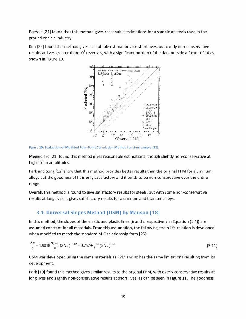
19

Roessle [24] found that this method gives reasonable estimations for a sample of steels used in the

ground vehicle industry.

Kim [22] found this method gives acceptable estimations for short lives, but overly non-conservative

results at lives greater than 104 reversals, with a significant portion of the data outside a factor of 10 as

shown in Figure 10.

Figure 10: Evaluation of Modified Four-Point Correlation Method for steel sample [22].

Meggiolaro [21] found this method gives reasonable estimations, though slightly non-conservative at

high strain amplitudes.

Park and Song [12] show that this method provides better results than the original FPM for aluminum

alloys but the goodness of fit is only satisfactory and it tends to be non-conservative over the entire

range.

Overall, this method is found to give satisfactory results for steels, but with some non-conservative

results at long lives. It gives satisfactory results for aluminum and titanium alloys.

3.4. Universal Slopes Method (USM) by Manson [18]

In this method, the slopes of the elastic and plastic lines (b and c respectively in Equation (1.4)) are

assumed constant for all materials. From this assumption, the following strain-life relation is developed,

when modified to match the standard M-C relationship form [25]:

0.12 0.6 0.61.9018 (2 ) 0.7579 (2 )2

UTSf f fN N

E

(3.11)

USM was developed using the same materials as FPM and so has the same limitations resulting from its

development.

Park [19] found this method gives similar results to the original FPM, with overly conservative results at

long lives and slightly non-conservative results at short lives, as can be seen in Figure 11. The goodness

20

for the data is 63% for all of the materials. This method gives similar results for all materials

classifications except for aluminum, where a few excessively non-conservative results are obtained.

Jeon [3] found similar results as Park.

Figure 11: Evaluation of Universal Slopes method for low alloy steels [19].

Kim [22] found this method gives reasonable results with 91% of the data with the factor of 3.

Similar to Park, Meggiolaro [21] found that this method gives non-conservative results at short lives and

highly conservative results for long lives.

Ong [20] showed that the correlation does not give very satisfactory results, with only 50% of the data

within a life factor of 3.

Park and Song [12] found the results from this method are reasonable for aluminum alloys, but the

goodness of fit is only 59%. The method is again found to be non-conservative at short lives and highly

conservative results for long lives.

3.5. Modified Universal Slopes Method (MUSM) by Muralidharan and

Manson [26]

MUSM uses the same assumptions as the original USM. However, the M-C parameters have been

modified to give more accurate results relative to the material sample used in its development. When

modified to match the standard M-C relationship form [25], the equation is:

0.832 0.09 0.155 0.53 0.560.623( ) (2 ) 0.0196 ( ) (2 )2

UTS UTSf f fN N

E E

(3.12)

The parameters from Equation (3.12) have been determined based on 47 materials, including steels and

aluminum and titanium alloys. Each of the parameters was determined using a least squares analysis.

Park [19] found that MUSM overcame most of the drawbacks of the original USM. It has a goodness of

fit of 75%, which is the highest of all of the methods that were tested. Therefore Park determined that it

21

gave the most satisfactory results of all methods. Additionally it gave the best results for unalloyed, low-

alloy and high-alloy steels. The method gives slightly conservative results at low lives and non-

conservative results at long lives as can be seen in Figure 12. For aluminum, a few excessively non-

conservative results are obtained at short lives.


Figure 12: Evaluation of Modified Universal Slopes Method for low alloy steels [19].



Kim [22] found this method gives some of the best estimations with 95% of the data within a factor of 3.

Meggiolaro [21] found this method gives reasonable results for steel. Significantly non-conservative

results may occur at small strain amplitudes (<1.0%). Meggiolaro notes that it should not be used for

aluminum or titanium alloys.

Park and Song [12] found that this method did not significantly improve upon the original USM for

aluminum alloys.

Lee and Song [27] found that this method provides the best results for steels and titanium alloys.

Overall, this method gives reasonable estimations for steels and provides some of the best estimates of

all of the methods.

3.6. Mitchell’s Method (MM) by Mitchell and Socie [28]

MM follows the standard form of the M-C relationship (1.4) [25], where:

' 345 ( )f f UTS MPa (3.13)

21log

6

f

UTS

b

(3.14)

22

' 1ln

1f f

RA

(3.15)

0.5 for ductile materials

0.6 for strong materials

c

c

(3.16)

These correlations have been developed only for steel with hardness below 500 HB.

Park [19] found that this method gives non-conservative results over the entire life range and

considerably non-conservative estimations in the longer life range, as can be seen in Figure 13. The

goodness of fit is 61% for all materials. This method was found to give the best results for aluminum

alloys; however it was developed only for steels.


Figure 13: Evaluation of Mitchell’s Method for low alloy steels [19].

Kim [22] found this method yields non-conservative results for nearly the entire life range, with only

66% of the data with a factor of 3.

Meggiolaro [21] found that this method does not give very good estimations.

Ong [20] found this method gave much poorer results than the other methods examined.

Park and Song [12] found that this method had a superior goodness of fit compared to the other

methods for aluminum alloys. As a result, this method was chosen to be improved upon for aluminum

alloys in the Modified Mitchell’s Method (MMM).

3.7. Modified Mitchell’s Method (MMM) by Park and Song [12]

In this method, MM is modified to make it more applicable for aluminum alloys. This method was

developed from a study using 16 aluminum alloys. It was found by Park [19] that MM provided the best

results of the available methods and so it was modified to more closely predict the results.

23

b 0.664UTSf f f

σ 335 ε(2N ) ε (2N )

2 E

(3.17)

UTS

UTS

σ 3351log

6 0.446σb

(3.18)

f can be estimated according to Equation (3.15).

Jeon [3] analyzed this method in a similar manner as Park, but only for aluminum and titanium alloys.

The sample of these alloys was very small, so caution with the results is advised. Jeon found that this

method had the best goodness of fit for both aluminum and titanium alloys, with goodness of fit of 74%

and 82% respectively.

Lee and Song [27] found that this method provides good results for titanium alloys.

Overall, this method appears to give satisfactory results for aluminum and titanium for which it is

applicable.

3.8. Medians Method (MedM) by Meggiolaro and Castro [21]

The development of MedM is based on the assumption that the median value for each of the M-C

parameters can be used for each material classification. MedM was developed under this assumption

using a sample of 845 materials, including 724 steels, 81 aluminum alloys and 15 titanium alloys, along

with small samples of Nickel alloys and cast irons. This method uses different models for each of the

material classifications. Meggiolaro found that 'f in particular was the parameter that was most poorly

estimated by other methods and that using the median values for each material classification provided

the best results. Using all of the experimentally obtained M-C parameters and a number of different

statistical models, the median value for each material class were determined. The parameters for each

of the models are shown in Table 1, which match the standard form for the M-C relationship given in

Equation (1.4).

Table 1: Calculated Manson-Coffin parameters for each material class for Median’s method [21].

'f '

f b c

Steels 1.5 UTS 0.45 0.09 0.59

Al alloys 1.9 UTS 0.28 0.11 0.66

Ti alloys 1.9 UTS 0.5 0.10 0.69

Ni alloys 1.4 UTS 0.15 0.08 0.59

Cast Irons 1.2 UTS 0.04 0.08 0.52

Meggiolaro notes that there is some temperature dependence for the εf’ values and further study may

be required.

This method has been developed using a large sample size, though the sample was strictly the M-C

parameters and not fatigue lives. As such the development is different than those by other authors. It

was developed to attempt to match M-C parameters and not the resulting fatigue life. Caution is advised

24

for the use of the method for titanium alloys, nickel alloys and cast iron due to the small sample size for

these materials.

Furthermore, Meggiolaro notes that if 'f is replaced by the median value in UML, HM or MUSM the

estimations improve marginally and the variability of the data is decreased.

Lee and Song [27] found that this method provides the best results for aluminum alloys and satisfactory

results for steel. It is however relatively poor for titanium alloys.

3.9. Method of Variable Slopes by Hatscher [29]

In this method, the fatigue exponents are not constant with life. This method is only applicable for

prestrained steel sheets and has divided steels into a number of subgroups, including high-strength,

mild, multiphase and austenitic steels and all of the steels used in the development have σUTS < 620 MPa

[25].

The equations that represent this method are summarized in [25], with full development and

explanation in [29]. It is not an applicable method since it is only for prestrained steel sheets and so it is

not discussed further.

3.10. Uniform Material Law (UML) by Bäumel and Seeger [30]

UML was developed using 125 different materials. The method was developed so that only readily

available properties ( UTS , E ) are required to allow for its easy use. It distinguishes between different

material classifications for the M-C parameters, with different classifications for steels and then for

aluminum and titanium alloys. Additionally, it was developed to include estimation of endurance limits,

the equations for which are in [30].

For unalloyed and low alloy steels:

0.087 0.581.50 (2 ) 0.59 (2 )2

UTSf fN N

E

(3.19)

Where UTSσ

1.0 for 0.003E

UTS UTSσ σ

(1.375 125.0 ) for 0.003E E

For aluminum and titanium alloys:

0.095 0.581.67 (2 ) 0.35(2 )2

UTSf fN N

E

(3.20)

Meggiolaro [21] notes that for steels, UTS must be less than ~2.2 GPa (with typical values of E ),

otherwise negative values of 'f will occur.

Park [19] found that this method was the second best method for the entire material range. The

goodness of fit in the factor of 3 life scatter bands is 74%. This method gives slightly conservative results

at lower lives and non-conservative estimations at longer lives as can be seen in Figure 14. Additionally,

25

this method is recommended by Park, especially when fracture ductility ( RA ) required for MUSM and

others is not available.

Figure 14: Evaluation of Uniform Material Law for low alloy steels [19].



Kim [22] found this method gives some of the best estimations with 93% of the data within a factor of 3.

Meggiolaro [21] found this method gives fair estimations, for steels and aluminum and titanium alloys.

Slightly non-conservative results may occur at large strain amplitudes for steels. This method was found

to give the best results for aluminum and titanium alloys.

Park and Song [12] show that this method gives some of the best results for aluminum alloys, similar to

the conclusions of Meggiolaro.

Lee and Song [27] found that this method provides good results for steels and for aluminum and

titanium alloys.

Overall UML was found by most of the researchers to give reasonable and satisfactory results, among

the best of the methods examined. Additionally, it gives reasonable estimations for steel and for

titanium and aluminum alloys. It is also easier to use since only UTS is required, as opposed to fracture

ductility required in many other methods.

3.11. Modified Uniform Material Law by Hatscher, Seeger and Zenner

[31]

In the Modified Uniform Material Law, a similar approach was taken as with the Method of Variable

Slopes to modifying the Uniform Material Law. Therefore slopes of the fatigue exponents are not

constant with life. This modified method has only been modified for steels, to match what was

26

determined for the Variable Slopes Method in [29]. The equations for this method are summarized in

[25] with the development given in [31]. It requires more information than just the monotonic

properties data and so it is not examined.

3.12. Hardness Method (HM) by Roessle and Fatemi [24]

In this method, the approach was to create a simple method for estimating the M-C parameters for

steels using only readily available properties: Brinell hardness and elastic modulus ( HB and E ).

2

0.09 0.56f f

4.25 HB 225 0.32 HB 487 191000ε(2N ) (2N )

2 E E

HB (3.21)

Other types of hardness could be used in this equation if necessary using appropriate correlations to

convert between hardness, some of which are presented in [27]. The fatigue strength and ductility

exponents (b and c) were taken to be the same as MUSM since similar results were found for the steels

studied.

This equation was developed based on a study of 69 steels total, the details of which are found in

Section 3.15 Overview of Comparison Papers.

Kim [22] found this method gives some of the best estimations with 95% of the data within a factor of 3,

though it has fairly large variability.

Meggiolaro [21] found this method gives reasonable results. Significantly non-conservative results may

occur at small strain amplitudes (<1.0%).

Lee and Song [27] found that this method provides the second best results for steels.

Overall, this mention is found to give reasonable estimations for steels, for which it is applicable. It is

also simple, in that only the hardness and elastic modulus are required.

3.13. Indirect Hardness Method by Lee and Song [27]

In this method, Lee and Song use a similar approach as Roessle to estimate the M-C parameters from

hardness values. However, they try and do this indirectly by using various correlations for estimating

UTS from different hardness measurements (Vickers hardness ( HV ), Brinell hardness ( HB ), Rockwell

hardness ( HRC )). Then the estimated UTS is used in some of the other estimation methods which only

require UTS as input (UML, MedM) to get the M-C parameters. This means there are a few different

combinations of correlations for estimating UTS from hardness and the M-C parameters from UTS . All

of the combinations analyzed are presented in [27]. If these methods are required, the necessary details

are also provided there.

These indirect hardness methods are compared versus HM by Roessle and Fatemi.

The applicability of these sets of equations is only when some of the properties such as f or UTS are

not available from experiment and therefore the other estimation methods cannot be used. In this case

27

indirect hardness can give estimation of the results. However, when UTS is available, UML or MedM

gives more satisfactory results. Since there are generally two different sets of correlations (to obtain

UTS from hardness and M-C parameters from σUTS) this may lead to significant error.

A total of 139 materials, including unalloyed, low-alloyed and high alloyed steels, and aluminum and

titanium alloys were used in the comparison.

This method is not well studied, however, Lee and Song found that the results obtained for most of the

indirect methods were comparable to the other methods, but the other methods provided slightly

better results.

3.14. Approach by Basan et al. [32]

In this method, Basan et al. find that there is no link between any of the M-C parameters, except 'f

and any monotonic properties data. Therefore 'f , b and c are independent of monotonic material

properties and 'f is found to be related to Brinell hardness. Therefore they take an approach similar to

MedM and these M-C parameters are constant. However, the difference is that they have different

properties dependent on the hardness of the material. Table 2 shows the M-C parameters based on

hardness. This is only applicable for steels.

Table 2: Manson-Coffin parameters versus Brinell hardness, from Basan et al. [32]

This method is not used in this research because of the limited scope of the results. The published

results just appear to be a summary of the M-C parameters for the materials in their study. This does

not give confidence that it could be utilized to estimate properties for other materials. Additionally, the

nature of the values given means that either results need to be interpolated, which does not seem

prudent given that the values fluctuate up and down or there is very limited applicability for the results.

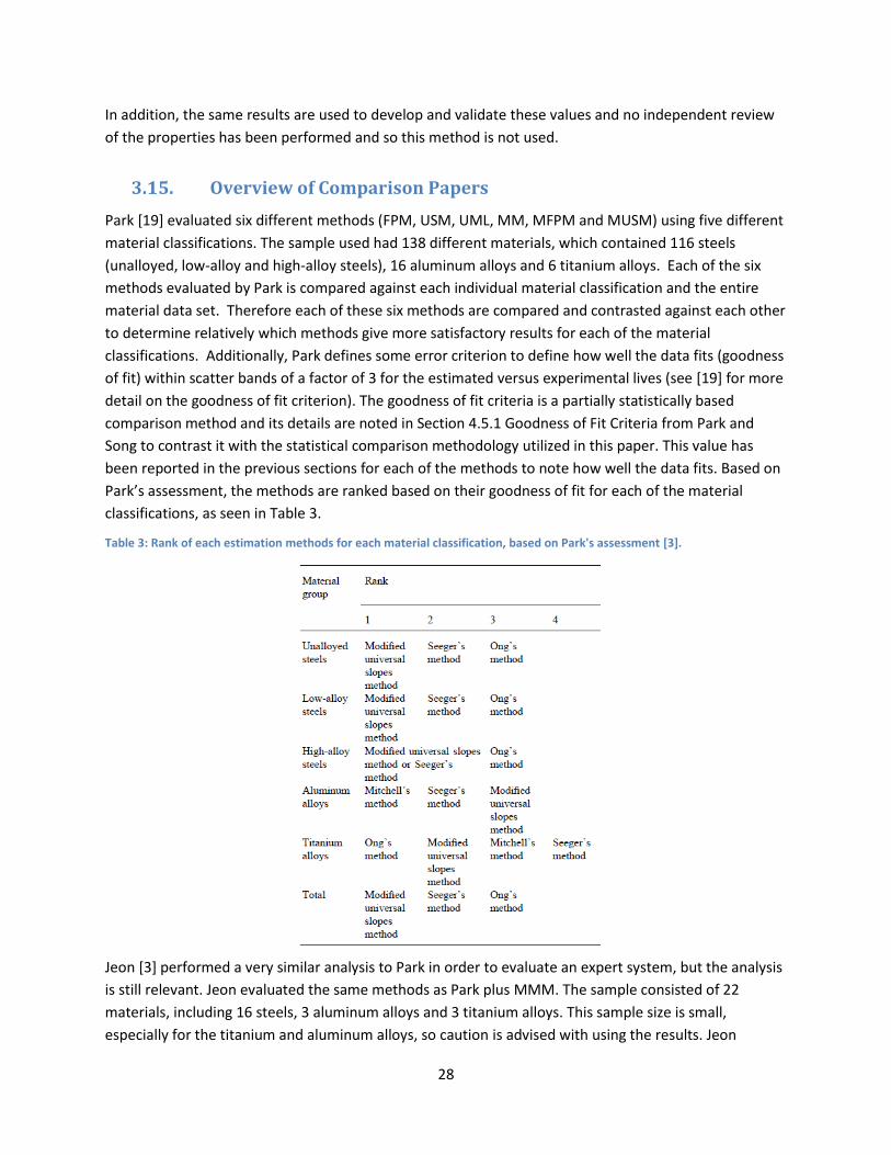
28

In addition, the same results are used to develop and validate these values and no independent review

of the properties has been performed and so this method is not used.

3.15. Overview of Comparison Papers

Park [19] evaluated six different methods (FPM, USM, UML, MM, MFPM and MUSM) using five different

material classifications. The sample used had 138 different materials, which contained 116 steels

(unalloyed, low-alloy and high-alloy steels), 16 aluminum alloys and 6 titanium alloys. Each of the six

methods evaluated by Park is compared against each individual material classification and the entire

material data set. Therefore each of these six methods are compared and contrasted against each other

to determine relatively which methods give more satisfactory results for each of the material

classifications. Additionally, Park defines some error criterion to define how well the data fits (goodness

of fit) within scatter bands of a factor of 3 for the estimated versus experimental lives (see [19] for more

detail on the goodness of fit criterion). The goodness of fit criteria is a partially statistically based

comparison method and its details are noted in Section 4.5.1 Goodness of Fit Criteria from Park and

Song to contrast it with the statistical comparison methodology utilized in this paper. This value has

been reported in the previous sections for each of the methods to note how well the data fits. Based on

Park’s assessment, the methods are ranked based on their goodness of fit for each of the material

classifications, as seen in Table 3.

Table 3: Rank of each estimation methods for each material classification, based on Park's assessment [3].

Jeon [3] performed a very similar analysis to Park in order to evaluate an expert system, but the analysis

is still relevant. Jeon evaluated the same methods as Park plus MMM. The sample consisted of 22

materials, including 16 steels, 3 aluminum alloys and 3 titanium alloys. This sample size is small,

especially for the titanium and aluminum alloys, so caution is advised with using the results. Jeon

29

obtained very similar results to Park for unalloyed steels, low-alloyed steels and high alloy steels. The

results are somewhat poorer for aluminum alloys, with the small sample size, but it was found that the

MMM had the best results. For titanium alloys, the results were similar, except that the MMM had the

best results.

Roessle and Fatemi [24] compared the method they developed (HM) to the MUSM, UML and MFPM,

which are the best methods as suggested by Park [19]. Using a sample of 69 steels common in the

ground vehicle industry, they compared these methods. These steels included a variety of processing

conditions. The method is valid for hardness from 150 to 700 HB. Other properties of the sample are

given in [24]. Roessle found that all three methods resulted in reasonable estimations. They found that

HM gave slightly better results than the other methods; however it should be noted that the data used

to develop HM and to compare the different methods was the same, therefore resulting in significant

bias towards HM.

Kim [22] compared the FPM, USM, MM, UML, MUSM, MFPM and HM, using a sample of 8 steels. All of

the steels can be considered ductile. MUSM, UML and HM were found to give the best results. Based on

this, Kim found that the constant fatigue strength and fatigue ductility coefficients ( b and c ), which are

all approximately the same among the three methods for steels, provide a reasonable estimation.

Meggiolaro [21] used a sample of 845 metals, including 724 steels, 81 aluminum alloys, 15 titanium

alloys, 16 cast irons and 9 nickel alloys to develop MedM and compare other estimation methods. These

include: USM, MUSM, UML, HM, MM, FPM and MFPM. Meggiolaro found that 'f in particular was the

parameter that was most poorly estimated by the other methods and does not correlate well with any

monotonic properties. Therefore using the median values for each material classification provided the

best results. In comparing each of the above mentioned models, Meggiolaro compared the estimation

of each of the M-C parameters to determine how well they correlated to the experimental data.

However, since the methods need to be considered in their entirety, the estimated lives for each

method should to be compared. One limitation of this sample is that the experimental results used are

the individual M-C parameters and not experimental lives, and therefore the experimental lives need to

be calculated. However, MedM was only compared on the basis of the M-C parameter values.

Meggiolaro found that MedM, UML and MUSM respectively gave the best results, while the other

methods evaluated give poorer results. Given that same data was used to calibrate MedM and to

compare it to other methods, there is a bias towards MedM.

Ong [20] used 49 steel samples for comparison of the FPM, USM and MM, in addition to developing

MFPM. This steel sample had properties that ranged from 300 to 2500 MPa for tensile strength, 10 to

80% for reduction in area and cyclically hardened and softened materials. Ong determined that FPM

gave the best results of those examined, and modified it to improve the results, thus MFPM. However,

none of the methods provided overly satisfactory results. In creating MFPM, Ong [23] used the same

steel sample as in [20]. Therefore, MFPM was calibrated and then evaluated using the same data set,

creating a significant bias in the analysis given in [23].

Park and Song [12] used 16 aluminum alloys (same aluminum data as [19]) to compare how well the

following methods estimated the life for aluminum alloys: FPM, USM, MM, MUSM, UML, MFPM and the

30

developed method, MMM. MM and UML give reasonable estimations, along with MMM, however it has

been calibrated and evaluated using the same data and so there is bias in this analysis.

Lee and Song [27] studied a sample of 52 materials, with 43 steels divided into unalloyed, low-alloy and

high-alloy classifications and 6 aluminum alloys and 3 titanium alloys. They compared HM (for steels

only), MUSM, UML and MedM. Additionally they also used numerous correlations to determine UTS

from hardness and then used this UTS in many of estimation methods. These methods are termed

Indirect Hardness methods. It was found that in general, the Indirect Hardness methods provided

reasonable results, but the other methods were more successful. However these Indirect Hardness

methods may be useful when only the hardness of a material is known.

Basan [25] looked into how the different methods treat material classifications and how this affects the

life estimation. Basan found that substantial differences in the M-C parameters exist between different

material classifications. This was done by comparing all of the M-C parameters and looking at

correlations based on material classification. This was done with a sample of 310 materials, which

include: 128 unalloyed steels, 64 low-alloy steels, 75 high alloy steels, 30 aluminum alloys and 13

titanium alloys. Therefore, Basan recommends that a differential approach is desirable for estimation of

M-C parameters. It is noted that estimation methods that employ a differentiation of materials provide

more accurate and reliable estimations if properly developed and calibrated. Therefore the MedM and

UML were recommended based on their approach.

3.16. Expert Systems

As was mentioned in the introduction, other researchers have created expert systems to assist a design

engineer in getting estimates for the fatigue properties. In these expert systems, various rules are

utilized to dictate which estimation method should be chosen for the particular material to be analyzed.

The goal of the expert systems is to enable a design engineer to use the selection of estimation methods

to determine the M-C parameters. They assist the design engineer by taking the onus to know the

limitations and which estimation methods work best for a material classification away from the

engineer. This is of practical importance, since as was seen in the previous section with all of the

comparison papers, there is a lot of information and knowledge to be acquired. The development of

expert systems is one important part of what is needed for more design engineers to have confidence

and the ability to use estimation methods for the many benefits to the design process.

While the expert systems have a lot of practical applications and benefits, and in essence an expert

system will be developed as a part of this research (see Section 9 Fatigue Properties Estimation

Software), each of the available expert systems have their drawbacks. Many of these drawbacks are

directly linked to the drawbacks that were mentioned above with regards to the comparison papers, as

the expert methods are derived from these comparisons. The first drawback is that all of the expert

systems are based on finding an estimation method that works best for a given material classification.

They only segment materials into classifications such as steel, aluminum etc or potentially low-alloy

steel, medium carbon steel etc. They do not however look at materials in terms of different heat

treatments. The estimation method that works best for one material is not necessarily the same as for

31

the next material. Therefore, with larger material classifications, there is going to be larger discrepancies

between results for multiple material grades. The best estimation method for that material

classification, therefore will give the best results on average, but on an individual material grade, the

estimation will be worse. Therefore having smaller material classifications, with more similarity of

properties will allow better estimations. This is the major basis for comparing the estimation methods

based on their heat treatment as will be done in this research.

Another aspect of the fatigue problem that is not considered for the expert systems and in all of the

comparison papers is the R-O parameters. The R-O parameters are of vital importance in the fatigue

problem, as in a majority of situation the stress is known and so the strain needs to be determined.

Without the R-O parameters, the life estimate cannot be made. The R-O parameters also need to be

considered and estimated, as is done in this work.

The expert system by Park et al. [4] uses results from Meggiolaro and Castro [21], Lee and Song [27] ,

Kim et al. [22], Park and Song [19] and Roessle and Fatemi [24] as the basis for their rules in the expert

system. However, a detailed explanation of the rules is not given and the results from the various

authors often have some conflicts as to which are the best estimation method for a particular material

classicisation. The expert system by Basan et al. [1] does not list the rules used in their system but

mentions the use of all of the comparison papers that have been previously discussed. The expert

system by Jeon and Song [3] uses the results from Park et al. [19] as the rules for the expert system.

Finally, the expert system by Lee and Song [2] uses the results from Jeon and Song [3] and Lee and Song

[27] as the basis for the rules in their expert system.

3.17. Summary of Literature

Numerous researchers have been involved with the development of the estimation methods and then

the comparison of the various estimation methods to determine which are the best for different

material classifications. Additionally, other researchers have recognized the value of these estimation

methods for the preliminary stages of a design process and have developed expert systems to

summarize this knowledge to make it practically possible for a design engineer to utilize. All of this is

very important contribution and this research will look to build on a lot of the previous work done.

However, there are some aspects of the previous research that need to be reconsidered and improved

upon as will be done in this research.

The previous research generally compared the estimation methods within large material

classifications. In this research, smaller heat treatment classifications for steels will be used. The

different heat treatment classifications can be used to provide more accurate results as the

properties of the material will be more similar and therefore the estimation methods chosen

will be more accurate.

The statistical method for determining the best estimation method needs to be improved upon,

as the previous methods do not have a strong enough statistical basis. The current statistical

methods use either percentage of points in scatter bands or arbitrary combinations of the

regression parameters. The scatter bands approach strictly gives the average result for the large

material classification. It does not look at the individual material grades. Additionally, the trend

32

of the life estimates is not accounted for and so it only looks at the individual experimental

points. The approach by Park et al [19] uses the linear regression. However, the goodness of fit

criteria somewhat arbitrarily uses these regression parameters to define the best linear

regression and therefore estimation method. These are not sound analysis techniques with

multiple drawbacks. A different statistical method will be used in this research, as will be

discussed in the next section.

The R-O parameters also need to be considered in addition to the M-C parameters. The R-O

parameters are necessary for almost any fatigue problem, but all of the other researchers with

their comparisons and expert systems ignore this important aspect. The R-O parameters will be

considered and examined in detail in this work.

In addition variability is considered in this work, to take the estimation methods one step

further.

33

4. Comparison of Estimation Methods – Manson-Coffin Parameters

One of the primary objectives of this research is to determine which estimation method gives the best

estimates of the lives and stresses by way of the estimates of the M-C and R-O parameters respectively,

for each of the heat treatment classifications discussed above. To accomplish this objective, material

data files from Deere & Company (John Deere) are analyzed. The number of data sets and the total

number of data points used are given in Table 4. A description of what is contained in these data files

and how it has been collected will be discussed below.

Table 4: Number of data sets and data points for each of the heat treatment classifications.

Heat Treatment Classification Number of

Datasets

Number of

Data Points Austempered Steel 3 44

Carburized Steel 3 44

Ferrite-Pearlite Steel 10 179

Incomplete-Hardened Steel 4 66

Martensite-Lightly Tempered Steel 4 68

Martensite-Tempered Steel 6 95

Micro-Alloyed Steel 4 65

Total 34 561

For each of the material data files, and at each strain amplitude for which testing was performed, the

estimated life ( theorN f ) is calculated from the M-C parameters from each of the estimation methods.

Additionally, from the experimental data, experimental M-C parameters can be fit using the standard

approach, which has been discussed in Section 1.1 Strain-Life Method. From these experimental M-C

values, experimental regression lives ( exp regN f ) can be calculated at each strain amplitude. A linear

regression is fit between the lives from each estimation method and the experimental lives ( expN f ) and

additionally between the lives from the experimental M-C parameters and the experimental lives. The

regressions for the estimation methods are then compared to the experimental regression for each

material grade. In determining which of the estimation methods gives the best results, a criterion is

necessary and it will be discussed in Section 4.5 Criterion for Comparison of Estimation Method. This

criteria looks at the difference in life estimates between the experimental regression life and the

estimation method life, at each experimental life, through the linear regressions.

The estimation methods are first compared for each individual material grade to determine individually

which estimation method gives the best results and statistical evidence is collected to indicate how close

these estimates are. Then all of the statistical information for all of the material grades in a heat

treatment classification is gathered together and the statistical information can be averaged across all of

these material grades. This is done to determine on average which estimation method is giving the best

results, along with the information for the individual material grades. Additionally, material grades

34

which are outliers or have differences in their results due to certain material properties can be

examined.

After each of the individual material data files has been analyzed, the materials data points are grouped

by heat treatment classification. Similar statistical analysis and the same comparison criteria are utilized

for the combined dataset. This is done to see how well all of the individual material grades and their

corresponding life estimates compare within the heat treatment classification. This is to ensure that the

basic assumption that all materials in a heat treatment classification will have similar characteristics for

their fatigue properties and therefore one estimation method will predominately give better results for

this heat treatment; is valid. Additionally, it helps to provide more evidence for which estimation

method gives the best result for each individual heat treatment. Consistency of results, between

individual material grades in a heat treatment, is very important for the best estimation methods.

All of this analysis will be discussed in more detail in subsequent sections. The results themselves will be

discussed in Section 5 Comparison of Estimation Methods for each Heat Treatment- Manson-Coffin

Parameters.

4.1. Strain-Life Testing Data

The material properties data that is available for each of the material grades (datasets), listed in Table 4,

consists of two portions: monotonic properties data and strain-life fatigue testing data. The data that is

included and the manner in which it was collected will be discussed briefly below.

The monotonic properties data generally consists of the following:

Elastic (Monotonic) Modulus ( E )

Ultimate Strength ( UTS )

Yield Strength ( ys )

Strength Coefficient ( K )

Strain Hardening Exponent ( n )

Reduction in Area ( RA )

Elongation ( Le )

Material Hardness, Brinell ( HB ) and Rockwell ( HRC )

This is the data available, however not all of it will be used in the analysis as will be discussed below. All

of the data, except the hardness values is collected from a tensile test. The tensile test is performed

according to ASTM Standard E8: Standard Test Methods for Tension Testing of Metallic Materials [33].

From the tensile test up to fracture the Elastic Modulus, Ultimate Strength and Yield Strength can be

determined. From measuring the dimensions of the fractured specimen, the Reduction in Area and the

Elongation can be determined. The strength coefficient and strain hardening exponent can be

determined from fitting the R-O curve to the tensile test stress-strain data. The hardness testing is done

according to ASTM Standard E18: Standard Test Methods for Rockwell Hardness of Metallic Materials

[34] for Rockwell hardness and ASTM Standard E10: Standard Test Methods for Brinell Hardness of

Metallic Materials [35] for Brinell hardness.

35

The data that is used out of this collection is the following, all of which are used as monotonic properties

data in one or more of the estimation methods, to determine the M-C parameters.

Elastic (Monotonic) Modulus ( E )

Ultimate Strength ( UTS )

Reduction in Area ( RA )

Brinell hardness ( HB )

The second portion of the testing data consists of the strain-life fatigue testing data. The fatigue test

data is collected according to ASTM Standard E606: Standard Test Method for Strain-Controlled Fatigue

Testing [7]. This data consists of a summary of the fatigue tests made on one set of material specimens,

with multiple test made at multiple strain amplitudes.

At each strain amplitude the following data is available:

Total strain amplitude (2

)

½ Life Stress ( exp )

Fatigue Life (reversals) ( expN f )

Cyclic Modulus

1st cycle stress

From this data, the strain amplitude and fatigue life are used for evaluating the estimation methods for

M-C parameters. The stress value is used for the R-O parameter comparison as will be discussed in

Section 6 Estimation of Ramberg-Osgood Parameters. The fatigue lives are the experimental lives and

the strain amplitudes are the values at which all of the estimation method lives are calculated for that

particular material grade.

The monotonic properties data and the fatigue testing data was collected on the same set of material

specimens.

4.1.1. Hardness from Ultimate Tensile Strength

For the material data files available in this research, both UTS and HB are available. However, in

practical applications the hardness may not always be available. Product information sheets from steel

manufacturers/distributers do not always contain the hardness. They do, however, almost always

contain UTS . Without hardness, HM cannot be used. From the literature review in Section 3.12

Hardness Method (HM) by Roessle and Fatemi and as will be seen in later sections, HM can give some of

the best results for certain heat treatment classifications.

There are correlations that are used to convert ultimate tensile strength to hardness and vice versa.

Therefore, it would be beneficial if HM could be used by converting the known UTS to HB . One such

correlation was proposed by Roessle and Fatemi in their paper [24] .

2

0.0012 3.3UTS HB HB (4.1)

This can be inversely written as follows, taking only the applicable result:

36

3.3 10.89 0.0048

0.0024

UTSHB

(4.2)

Therefore, if only UTS is known, it can be converted to HB and then HM used.

The accuracy of results obtained by using this conversion needs to be verified. The first step is to

compare the actual measured HB values to those estimated by using Equation (4.2). This comparison is

seen in Figure 15. As can be seen, the measured and estimated values are very close to being equal.

There are three points which are exceptions and these three points are for the three carburized

materials in the data files. The fact that the carburized material grades do not match this correlation is

expected, as the surface layer of the material is hardened by the carburizing process, as has been

detailed in Section 2.2.5 Carburized Steel. The hardness measurement is determined from the grains on

the surface of the material, which have been hardened by carburizing. Therefore, the hardness increases

significantly. However, carburizing does not affect the core of the material. This core of the material is

what primarily influences the UTS value. Since HB is being influenced by carburizing and UTS is not, then

it is expected that the relationship does not hold.

The remainder of the estimated hardness values are very close. The typical error between the values is

within 5% , with maximum error at 20%. Therefore the estimated hardness values are reasonably

accurate.

Figure 15: Comparison of measured hardness values to estimated values from ultimate tensile strength, for all material grades in this research.

While this comparison shows that the estimated hardness values are close to the measured ones, it

does not conclusively prove that there will be no effect on the M-C parameters determined by HM using

the estimated HB values. Therefore, in Section 5.1.1 Manson-Coffin Parameters from Estimated and

Measured Hardness, the results for the life estimations using M-C parameters determined from the

measured and estimated hardness values will be compared. This will be used to determine if it is

appropriate to use estimated hardness values when measured values are not available.

0

100

200

300

400

500

600

700

800

0 200 400 600 800

Esti

mat

ed

Har

dn

ess

[H

B]

Measured Hardness [HB]

37

4.2. Estimation Method Calculations

With the monotonic properties data obtained from testing, the M-C parameters for each estimation

method are calculated/estimated using the equations presented in the appropriate subsection of

Section 3 Literature Review. It is noted that for MFPM, the estimate for f is given by Equation (3.2).

For USM, MUSM and MM, the estimate for f is given by Equation (3.8). With these equations, all of the

M-C parameters are known for each estimation method.

With the M-C parameters and the strain from the experimental testing file, the life can be iteratively

solved using the M-C relationship (1.4). This is done for each estimation method and each strain level.

This gives an estimated life at each strain level and for each estimation method, to be compared to the

experimental regression life.

An overview of this comparison is seen in Figure 16. This figure shows how the data from testing and the

estimation methods are used to get estimated lives and experimental regression lives. Then the linear

regressions are created versus the experimental lives. Finally the estimated lives regressions are

contrasted against the regression from the experimental regression lives and multiple contrasts is used

to determine the best estimation method for that material grade. Then across all material grades in a

heat treatment classification, it is repeated and the overall best estimation method for that classification

can be determined.

More details on the procedure will follow, but this figure shows the procedure that will be followed with

this analysis.

Figure 16: Overview of the statistical analysis methodology used to determine the best estimation method for each heat treatment classification.

38

4.3. Analysis of Testing Data

There are a large number of material datasets available for this research (listed in Table 4) and within

these there are a large number of data points that can be analyzed. All of these data points have been

experimentally obtained, as has been detailed in Section 4.1 Strain-Life Testing Data. However, in this

data, as with any experimental data, there are data points which do not match the other data and can

be said to have experimental error. Removing these types of data points, when appropriate, will allow

the analysis to give much clearer results, instead of the results being clouded in uncertainty. With that

being said, data points cannot just be arbitrarily removed, as every data points contains information that

may be useful for the analysis. Additionally, some differences in the data are appropriate and expected,

as there is a certain amount of variability in every material property, especially fatigue properties. As a

result, only significantly erroneous data is removed.

In this project, to determine which experimental points are appropriate, the points are first screened

through a piece of software, FALIN, involving the strain-life fatigue approach and can be used to analyze

material data. This will be discussed below. Additionally, there are a few other cases for which data

points or datasets are removed from the analysis.

Within the material data files, certain data points are indicated as runout data. Runout data occurs when

the test is stopped because the specimen has exhibited a specified life, and therefore testing time,

which exceeds that available for the testing. This indicates that at that particular strain level, the

specimen achieves near infinite life. Since these lives are not true lives, as the defined fatigue failure did

not occur ( 0.5mm crack), they are excluded from the analysis.

Certain entire datasets are excluded if all of the necessary monotonic properties are not available, such

as RA , UTS etc. Without these necessary material properties, not all of the estimation methods can be

utilized and so they cannot be compared. Without being able to compare all of the estimation methods,

the objectives cannot be met and so these datasets are excluded.

Additionally, plastic strain values are excluded if they are below an established limit (threshold) 0 . The

reason for having a strain threshold is because of the accuracy of the plastic strains below this threshold.

The threshold chosen is 0 0.01% . This is the threshold value utilized by other authors [6] and

indicated as the uncertainty in the total strain measurement [36]. The reason for a plastic strain

threshold has been discussed in [36]. One major reason is that the plastic strain is determined by

calculating the elastic strain from the measured stress and then subtracting the elastic strain from the

total strain to get the plastic strain. Therefore the plastic strain is not measured directly and is strongly

influenced by the elastic strain term. Therefore at very small plastic strains, a slight change in the elastic

strain (stress) value has a significant influence on the plastic strain. Therefore the plastic strain threshold

is utilized to eliminate these issues.

4.3.1. FALIN

FALIN is a software “program for fatigue life estimations based on notch-strain approach” [37]. It can be

used to predict the fatigue life of a component given its geometry, loading history and material

39

properties. It utilizes the strain-life methodology. In this research, only its material properties

functionalities are utilized. The material properties are fit according to the ASTM standard [13]. It is used

to determine the experimental M-C parameters for each individual material dataset, from the

experimental data. The procedure to determine the M-C parameters is explained in Section 1.1 Strain-

Life Method. The experimental M-C parameters are the best values that can be achieved, given the

experimental data. The estimation method M-C parameters are compared to these values, through the

fatigue life, as will be discussed in subsequent sections. The coefficient of variation (COV) for the fatigue

strength and ductility coefficients ( 'f and '

f respectively) will be utilized in Section 8.3 Fatigue

Properties Variability from Testing as will be discussed there.

Additionally, in this portion of the analysis, FALIN is used to determine which experimental points do not

fit compared to the rest of the data and those below the plastic strain threshold, 0 .

To determine the M-C parameters, and subsequently decide which points are excluded in the fitting

process, the total strain, stress and fatigue life are entered into the program, along with the elastic

modulus ( E ). First the plastic strain points below the plastic strain threshold, 0 are excluded. Secondly

runout data is excluded, as the final life is unknown. Other experimental points are removed if they are

outliers within the data. Since the strain amplitude is the independent variable and the life and stress

are dependent, the life and stress values are analyzed to determine if they are outliers. With decreasing

strain amplitudes, the life should increase and the stress should decrease. If there are any data points

which do not fit this behavior and deviate significantly, they are removed. An example is, if the life for a

certain strain amplitude is significantly shorter than the life seen for a higher strain amplitude, this point

would potentially be removed.

These outlier values can be determined by fitting a linear regression to the data (elastic and plastic

strain versus life) and determining the experimental regression M-C parameters. With these parameters

and the independent strain amplitude, the experimental regression life can be calculated. This

experimental regression life can be compared to the experimental life. If these values are significantly

different, then the life is probably an outlier data point. This data point is removed and the regressions

can be fit again, giving different M-C parameters. The experimental regression lives can then be

recalculated for every strain amplitude except that corresponding to the removed data point. These new

experimental regression lives can be compared to the experimental regression lives calculated with the

previous regression. If there was a significant change to the lives, then the removed data point was

influential and therefore was an outlier.

This is a very similar approach to Cook’s Distance [38], where the influence of removing a data point is

checked. In this case the changes in the life values are compared instead of the change in the linear

regression parameter. The same thing can be done with the stresses. The goal is to have as many

relevant data points as possible, but if they are clouding or causing inaccuracies in the results, they are

excluded.

When using the R-O curve, there is always a plastic portion to the strain. However, before the stress

approaches the yield stress, only elastic strain should occur. In reality the plastic strain is very small, but

is not 0. From looking at the R-O curve, these points fall on the nearly straight portion of the curve

40

before it curves to the plastic strain portion. These are the points that are generally below the plastic

strain threshold, 0 . Additionally, since the stress value used is experimentally determined, it can be

found that for this stress value, the elastic strain is slightly larger than the strain value from the

experiment. Therefore the plastic strain would be negative. These points may be removed since the

stress value is incorrect or the plastic strain value will be removed since negative values are not possible.

As a result, for the plastic strain versus life curves, plastic strains that are very small, or negative and

should be 0 are removed from the analysis. These points are kept in the elastic strain versus life curve.

4.4. Statistical Analysis

As is mentioned in the introduction section, the accuracy of the estimation methods is assessed by

comparing the linear regressions of each estimation method to the linear regression from the

experimental M-C values. The linear regressions are created by plotting the estimated lives versus the

experimental lives. For each material, there are a number of different strain levels, and therefore lives,

and so a simple linear regression is fit to the data. This provides a correlation to indicate how closely the

estimated life is to the experimental life. The model for the simple linear regression is given by:

theor explog( ) log( )f fN N (4.3)

The lives are compared on the basis of the logarithm of lives so that equal weighting is given to lives in

each decade. If the estimated life matched the experimental life, for all strain levels in the experimental

testing, then there would be a perfect correlation and 1 and 0 would occur. In this case it would

not matter if a linear regression or logarithmic regression were used, but as soon as there is deviation

from these values, then the logarithmic regression needs to be used.

For example, if an estimated life is different by a factor of 2 from the experimental regression life, it

should result in the same deviation from the perfect regression, regardless of the value of the life. This is

not true if the regression is done on a linear scale but it is true if it is done on a logarithmic scale. A proof

for this is given below:

For a simple linear regression, the best fit is found by minimizing the sum of squared errors (SSE)

2ˆ( )SSE Y Y

For a linear relationship Y X

For a linear regression where Y X , 1

0

.

If there are a large number of points, all which have i iY X and one point that is 2n nY X , then the

regression parameters will still be 1

0

.

22 2 2 2ˆ( ) ( ) [2 ( )] [ (1 ) ] [ ]n n n n n n n n nY Y Y X X X X X X

Therefore 2( )nSSE X , since 2ˆ( ) 0Y Y for every other point.

41

If a logarithmic relationship is used, ˆlog( ) log( )Y X

If there are a large number of points, all which have log( ) log( )i iY X and one point that is

log( ) log(2 )n nY X , then the regression parameters will still be 1

0

.

22 2 2

2 2

ˆ(log( ) log( )) log( ) ( log( ) ) [log(2 ) ( log( ) )] [log(2) log( ) ( log( ) )]

[log(2) (1 ) log( ) ] [log(2)]

n n n n n n n n

n

Y Y Y X X X X X

X

Therefore 2log(2)SSE

Therefore, this shows that for a linear regression, the decade of the point has an influence on the sum of

square error, while with a logarithmic regression it does not. Therefore for the logarithmic regression

equal weighting is given to lives in each decade, while this does not occur with a linear regression. Due

to the fact that with a small number of points, and will be changed in order to minimize SSE , there

will be some effect based on the nX for the logarithmic regression. However, the effect for the linear

regression will be more significant as can be inducted from the above result. On this basis, the fatigue

lives, which vary over several orders of magnitude, need to be compared with a logarithmic regression.

In addition to a regression for each of the estimation method, there also needs to be regression for the

lives calculated from the experimental M-C values. As is mentioned in Section 1.1 Strain-Life Method,

due to the variability in the data and imperfect nature of the M-C relationship, there will be differences

between the experimental lives and the lives calculated from the experimental M-C parameters.

Therefore a linear regression is fit as follows.

exp reg explog( ) log( )f fN N (4.4)

How closely the regression for each estimation method matches the regression from the experimental

M-C parameters will be the basis for determining the best estimation method, as will be discussed later.

An example figure, plotting estimated versus experimental life (log-log scale), is shown in Figure 17. Also

shown is the regression (solid blue), perfect correlation line (solid black) and scatter bands of a factor of

2 on life (dotted black). The same thing is done for the regression from the experimental M-C

parameters, seen in Figure 18. For this regression, it should be fairly close to a perfect correlation,

notwithstanding the differences due to the imperfect relation and variability as discussed.

42

Figure 17: Estimated versus Experimental Life, with linear regression added. Hardness Method, Ferrite-Pearlite Steel.

Figure 18: Experimental Regression versus Experimental Life, with linear regression added. Hardness Method, Ferrite-Pearlite Steel.

The regression is calculated using the following model. The errors are assumed to be normally

distributed and can be checked using residual plots to ensure that this condition is met. All of the

following equations are taken from [38], simplified as necessary for simple regressions.

Y X (4.5)

where

1

2

n

y

yY

y

,

1

2

1

1

1 n

x

xX

x

, 0

1

,

1

2

n

.

1E+3

1E+4

1E+5

1E+6

1E+3 1E+4 1E+5 1E+6

Esti

mat

ed

Lif

e (

2N

f th

eor)

[re

v.]

Experimental Life (2Nf exp) [rev.]

1E+3

1E+4

1E+5

1E+6

1E+3 1E+4 1E+5 1E+6

Exp

eri

me

nta

l Re

gre

ssio

n L

ife

(2

Nf

exp

re

g)

[re

v.]


43

Note 0

1

from the definitions given in Equations (4.3) and (4.4).

The least squares estimator for is given by .

1ˆ X X X y

(4.6)

The residual sum of squares, SSE, is given by:

ˆSSE y y X y (4.7)

The regression sum of squares, SSR, is given by:

2ˆSSR X y ny (4.8)

The total sum of squares, SST, is given by:

2SST y y ny (4.9)

The degrees of freedom for each of these is given by:

SSEdf n p (4.10)

1 1SSRdf p

1SSTdf n

Where n is the number of data points in the linear regression and p is the number of parameters in the

linear regression. For a simple linear regression, 2p .

With the error terms calculated, the variance and the correlation coefficient 2R can be calculated.

2ˆSSE

n p

(4.11)

2 SSRR

SST (4.12)

The variance describes the variability of the data and in the case of a regression, the variability that is

not accounted for by the relationship implied by the regression. Therefore it is the variability about the

regression line. The correlation coefficient describes how well the regression fits the data by giving the

percentage of the error that is explained by the regression.

While both are good indicators of how well the linear regression fits the model, there are a number of

other tests that can be performed which more concretely indicate the significance of the linear

regression.

The approach that is used is ANOVA tables and confidence intervals. An ANOVA table is also called a

one-way or single-factor analysis of variance model [38]. An ANOVA table is a way to summarize the

source of variance in the data and to test whether there is a difference between the error variance and

the regression variance. The ANOVA table for the material and estimation method in the previous figure

44

is seen in Table 5. The Sum of Squares and Degrees of Freedom are calculated as given in Equations (4.7)

to (4.10). The Mean Squares is just division of the sum of squares by the degrees of freedom.

Table 5: ANOVA Table for linear regression for above material and estimation method. Hardness Method, Ferrite-Pearlite Steel.

ANOVA TABLE

Source of Variation SS df MS obsF

Regression 6.9093 1 6.9093 2256.67

Error 0.0490 16 0.0031

Total 6.9583 17

The obsF seen in Table 5, is used to evaluate the following hypothesis test, to determine if the linear

regression is significant.

0 1: 0H

1 1: 0H

The hypothesis test is evaluated by calculating:

obs

MSRF

MSE (4.13)

This obsF value is compared to the F-distribution, with 95% confidence, to determine if it is significant

and therefore is the null hypothesis is rejected. In this case 1, ,0.05 1,16,0.05 4.49crit p n pf f f .

obs critF f

0 reject H

This means that the regression line is significant and that the regression helps to explain the data.

A final statistical test that is calculated is a confidence interval for and . This is done to understand

the range to these values, given the variance in the data. A confidence interval is the interval where the

parameter would be expected to lie [38]. As will be seen later, the and parameters are used in one

comparison criterion to determine which estimation method gives the best result. The confidence

interval is calculated to understand how much variability there is in this comparison criterion.

The confidence interval, about the mean response ( or ), is calculated by the following:

12

2,n p iit X X

where 1 for i and 2 for i (4.14)

All of the above statistical values, tests and calculations are performed for each of the estimation

methods and for each of the materials and the values are summarized in the appropriate files. An

example summary table is as seen in Table 6.

45

Table 6: Summary of Statistical Values calculated for each estimation method and material. Ferrite-Pearlite Steel.

HM

Beta 0.9704

Alpha 0.0641

Total Diff. 0.43

s 0.0553

Ea 0.9671

R2 0.9930

Beta Int 0.0433

Alpha Int 0.2005

SSE 0.0490

SSR 6.9093

SST 6.9583

MSE 0.0031

MSR 6.9093

Fobs 2256.6748

Sig. TRUE

Finally, as is mentioned at the very start, the assumption that the errors are normally distributed needs

to be checked. This is to ensure that the model chosen is in fact correct. If the errors are not normally

distributed, or if there is a discernible trend to the errors on the residual plot, then the model may be

inadequate. The errors are calculated as the difference between the value as estimated by the model

and the true measurable value. The residual plot for the material and estimation method being

examined is seen in Figure 19. Additionally, to determine if the errors are normally distributed, a normal

probability plot is used. A normal probability plot for the errors in this case is seen in Figure 20.

Figure 19: Residual Plot, for correlation as given in Figure 17.

-0.150

-0.100

-0.050

0.000

0.050

0.100

0.150

1E+3 1E+4 1E+5 1E+6

Re

sid

ual

s


46

Figure 20: Normal Probability Plot for residuals given in Figure 19.

Figure 21: Residual Plot, for experimental Manson-Coffin parameters regression, given in Figure 18.

Figure 22: Normal Probability Plot, for experimental Manson-Coffin parameters regression, given in Figure 21.

R² = 0.9642

-0.2

-0.1

-0.1

0.0

0.1

0.1

0.2

-2.0 -1.5 -1.0 -0.5 0.0 0.5 1.0 1.5 2.0

Xi

Si

-0.200

-0.100

0.000

0.100

0.200

1E+3 1E+4 1E+5 1E+6

Re

sid

ual

s


R² = 0.9493

-0.2

-0.1

0.0

0.1

0.2

-2.0 -1.5 -1.0 -0.5 0.0 0.5 1.0 1.5 2.0

Xi

Si

47

As can be seen from the normal probability plot for both the estimation method and the experimental

regression, the errors appear to be normally distributed and there does not appear to be a significant

discernible trend to the residuals. Therefore the model is appropriate. This is as expected, as there

should be a relationship between the estimated and experimental lives. How close this relationship is to

the perfect correlation is the subject of the next section on comparison criterion.

All of the analysis as described above is calculated for each of the estimation methods and for each

material to gather a comprehensive look at each material for further analysis.

4.5. Criterion for Comparison of Estimation Method

To determine which estimation method provides the best results for a particular material grade

(dataset) or for a number of material grades within a material classification, there needs to be

quantitative criterion that can be used to compare the estimation methods. In a number of previous

papers on the subject, as discussed in Section 3 Literature Review, the criterion compares the estimation

methods based on the percentage of data that falls within a scatter band of a particular life factor.

Typical the life factor is 3. Another criterion, Goodness of Fit, was utilized by Park and Song and will be

discussed below. This approach is the closest to the approach being employed so it will be explained and

discussed. Both of these approaches can help to indicate the accuracy of an estimation method;

however they do not do so with strong statistical basis or provide quantitative statistical evidence to

reach definite conclusions. Finally, the criterion which is used in this project is a statistical based

multiple contrasts approach.

4.5.1. Goodness of Fit Criteria from Park and Song [19]

In their paper, Park and Song tried to utilize a criterion for comparing estimation methods which

removed some of the inherent problems in the previously employed error criterion. The percentage of

data points within the life scatter bands has the inherent problem that only the specific data points are

important and not the trend or regression that these data points created. However, through the use of a

regression it indicates how well the estimation method results would match the experimental results

over a specified life range. These problems are discussed, with supporting examples in their paper [19].

As a result of this major deficiency in the life scatter bands error criterion, Park and Song utilize a

criterion that focuses on the linear regression. They reason that how closely the linear regression of a

particular data set matches the perfect correlation ( 1 , 0 ) indicates the accuracy of an estimation

method [19]. Using this idea, they utilize , and ( ) , along with the correlation coefficient, r , as

values to be used to quantitatively compare the estimation methods. Using these parameters, they

developed the Goodness of Fit ( aE ) criterion. The Goodness of Fit criterion has different components

for individual data sets and for entire material classifications. Their criterion is meant to evaluate which

estimation method gives the best results for a material classification. In their study, the material

classifications were: unalloyed steels, low-alloyed steels, high-alloy steels, aluminum alloys and titanium

alloys.

The following is the overall criterion [19]:

48

( 3) ( ) ( )

3

f a total a DsetE s E EE

(4.15)

The terms in the overall criterion can be calculated by the following. The first term is the percentage of

data with the life scatter bands (factor of 3) and can be calculated as [19]:

1 PredNumber of data points falling within

Exp( 3)

Total number of data pointsf

ss

E s

(4.16)

The second term is the goodness of fit term of the linear regression for all datasets combined (contains

all data points in a material classification) [19]:

1 1 1 1 1 1 1( )

4

total total total total total

a total

rE

(4.17)

The third term is the average goodness of fit term across all individual datasets [19]:

1 1

1 1 1 1 1 1 11 1( )

4

N Ni i i i i

a Dset a ii i

rE E

N N

(4.18)

Therefore the overall Goodness of Fit criteria is composed of three parts, a goodness of fit for the

individual datasets, goodness of fit for the combined dataset and the percentage of data within the

scatter bands. Unfortunately, none of these three components have much of a statistical basis. The

percentage of data within the scatter bands has a statistical basis as an overview of the amount of data

within a certain range; however it has a number of inherent problems as were pointed out by Park and

Song in their paper and detailed briefly above. The Goodness of Fit criteria does not, however, have a

statistical basis. The ideas and thought process behind the criteria are sound, with the comparison of the

regression to a perfect correlation being an appropriate comparison. However, the manner in which the

two regressions are compared has no basis. The choice of which parameters to include in the criterion

are based on where deviation from a perfect correlation will occur and what combinations for the

parameters means the least significant deviation. The weighting for the intercept ( ) and slope ( ),

combination and the correlation coefficient ( r ) has been assigned as being equal. These choices were

made by the author and as such have no statistical basis. This significantly weakens the viability of this

as a criterion and others with a statistical basis will be investigated.

4.5.2. Multiple Contrasts from Spurrier [39]

In response to the limitations of the previous methods, it is necessary to locate and utilize an

appropriate statistical comparison. The comparison of multiple values, like the mean of numerous

samples, is a common contrast problem; however in this case the contrast is between regression lines

instead of single values. In his paper, Spurrier presents the development of a multiple comparison

method based on a parametric function, as opposed to comparing the means [39]. It is restricted to

simple linear regression lines, which matches the needs of this project as the logarithmic transformation

still results in a linear regression of the logarithm of the values. With this approach, three or more

49

regression lines can be compared, provided that the design matrix is the same [39]. This is appropriate

for this application because there are numerous regression lines (for each estimation method) that are

being compared to the experimental regression line. In this case the design matrix, which is the x

variable, is the experimental life and is therefore the same for all of the estimation methods and the

experimental regression line.

The multiple contrasts works for parametric function of the following form (simple linear regression)

with the assumption of normal errors, which is assumed and checked in the statistical analysis [39].

ij i i j ijY x (4.19)

The multiple contrasts can be performed using the following, with the confidence bands removed [39]:

1 2

2 2

1 1 1

1ˆˆ ˆ( ) ( )

k k k

i i i i i i i

i i i

c x c x b x cn

(4.20)

where k is the number of contrasts, b is a parameter for the confidence bounds, n is the number of

design points and c is the contrast vector which has the following restriction 1

0

k

i

i

c

.

This contrast has confidence bounds associated with it, which will also be used in this analysis. In this

project, there are eight (8) estimation methods and the regression from the experimental M-C values,

making the number of contrasts nine (9). The value of b is given in the paper in tabular form. As such,

for the individual material grade confidence intervals, the value of b needs to be interpolated based on

n . Even though there are nine (9) contrasts, the tabular data only goes to eight (8) contrasts and so to

avoid extrapolation, the value for eight (8) contrasts is used, which is conservative. For the confidence

intervals of the combined dataset, the number of data points tends to exceed the largest value in the

table and so the largest b value available from the paper is utilized. As the number of contrasts ( k ) and

n become large this value approaches a constant. As such the value of b is 4.253 [39]. The confidence

interval level is 95% [39].

When comparing each individual estimation method to the regression from the experimental M-C

values, they can be compared by setting all of the c values to 0, except for the ones corresponding to

the estimation method and the regression from the experimental M-C values, which are then -1 and +1

respectively. However, for calculating the b parameter the total number of contrasts (9) needs to be

used to get the appropriate confidence level, without a high level of error.

In using this multiple comparison method, the design matrix must be scaled and centred, which means

that the following are true [39]: 1 0x and 1x x .

For this project, the linear regression is in terms of the logarithm of the experimental life and estimated

life, and experimental life and experimental regression life. As a result, all of the calculations involving

the multiple comparisons are calculated in the logarithmic domain.

With Spurrier’s comparison method, the calculated parameter is the difference between the compared

regressions versus the x variable, which in this case is the experimental life. For this project, where the

50

compared regressions are the lives from the experimental regression M-C values to the regression for

each estimated method, the difference (in linear scale) becomes the experimental regression life divided

by the estimated life. This is illustrated by the following, where the difference is calculated from

Equation (4.20), with c for the regression from the experimental M-C parameters being +1 and -1 for the

estimation method.

log exp reg exp reg theor theor

exp reg

theor

Nlog

N

f

f

Difference x x

(4.21)

exp reg

theor

f

f

NDifference

N

(4.22)

With this observation, the difference calculated by Spurrier’s method is just the experimental regression

life divided by the estimated life, plotted against the experimental life. This means that the figure shows

how far apart the experimental regression and estimated life are for each life or life range. This is a very

useful observation to be able to see the life ranges where each estimation method gives the best

estimations. This can be seen in Figure 23 and it helps to show the better estimation methods. The dark

black line is used to indicate where no difference between the regressions would occur. A Difference

greater than 1 is conservative and less than 1 is non-conservative.

Figure 23: Difference of experimental and estimated life using Spurrier's multiple comparison method. Ferrite-Pearlite Steel.

This can then be plotted as the percentage difference between the experimental regression life and the

estimated life at each experimental life as follows:

0

1

10

1E+3 1E+4 1E+5 1E+6

Dif

fere

nce

(N

f exp

/Nf

theo

r)


FPM

MFPM

USM

MUSM

MM

MedM

UML

HM

Non-conservative

Conservative

51

theor exp reg

exp reg

theor

exp reg

Percentage Difference

1

11

f f

f

f

f

N N

N

N

N

Difference

(4.23)

Figure 24: Percentage difference of estimated life and experimental regression using Spurrier's multiple comparison method. Ferrite-Pearlite Steel.

Figure 24 shows the percentage difference between the estimated life and experimental regression life

over all of the experimental lives. It is noted that a negative (-) percentage difference means that the

estimated life is shorter than the experimental regression life and therefore the estimated life is

conservative. Zero (0) percentage difference is highlighted by a black line so that it is easier to identify

where the estimation methods cross from conservative to non-conservative and vice-versa.

However, the objective is to find a quantitative comparison criterion and this is still somewhat

qualitative from only looking at the figure. To make this quantitative, the solution is to take the area

between the percentage difference line and zero (0). Therefore, the absolute area under the curve is

calculated, with both areas above and below 0 being considered as positive area. This is so that if any

method that has positive and negative percentage difference, they do not cancel out. The area is

calculated using rectangle method for numerically integration, with the midpoint approximation being

used. Since the shape for which the area is being calculated approximates a triangle, the error will be

negligible with this numerical calculation.

This calculated area between the percentage difference line and 0 is termed Sum Difference and is

calculated for each estimation method. Additionally, the Sum Difference can also give you the absolute

average value of the percentage difference over the life range. This can be calculated as follows:

-100%

-50%

0%

50%

100%

1E+3 1E+4 1E+5 1E+6

Pe

rce

nta

ge D

iffe

ren

ce (

The

or.

fro

m E

xp.

Re

g.)


FPM

MFPM

USM

MUSM

MM

MedM

UML

HM

Non-conservative

Conservative

52

Sum DifferenceAverage Percentage Difference

log(Experimental Life Range)

(4.24)

Therefore to calculate the Average Percentage Difference, you just need to calculate the Sum Difference

and the life range. The Average Percentage Difference value is the one that is utilized for comparative

purposes. The Percentage Difference versus life charts are needed to determine if the Percentage

Difference is conservative, non-conservative or transitions between for each material. For the material

discussed above the Average Percentage Difference values are seen in Table 7 and from Figure 24 it can

be seen whether it is a positive or negative Percentage Difference. These Average Percentage Difference

values are ranked to show which the lowest value is.

Table 7: Average Percentage Difference for each of the estimation method. Ferrite-Pearlite Steel.

FPM MFPM USM MUSM MM MedM UML HM

Avg. Diff. (Indiv.) 22.4% 38.3% 28.3% 38.6% 76.0% 62.3% 36.9% 14.0%

Rank Avg. Diff. (Indiv.) 2 5 3 6 8 7 4 1

Therefore, Spurrier’s method and the calculation of the area under the curve are used to give a

statistically sound and quantitative method to analyze which estimation methods gives the best results.

Therefore, it is used in this research as the estimation method comparison criterion. The Average

Percentage Difference value and its rank will be used as quantitative measures of the best estimation

methods. The Percentage Difference curves are utilized to indicate consistency of the estimation

method and whether it is conservative or non-conservative.

4.6. Comparison of Estimation Methods within Heat Treatment

Classification

The statistical analysis presented in the previous sections, using the comparison of regressions by

multiple contrasts, to determine the best estimation method for each material grade is repeated for all

of the material grades in each heat treatment. Therefore all of the statistical values and curves, including

the percentage difference versus experimental life curve, as seen in Figure 24 and the Average

Percentage Difference values as seen in Table 7 are obtained for each of these material grades. The

Average Percentage Difference values for each material grade are ranked, indicating which estimation

method gives the lowest Average Percentage Difference.

Then across all of the material grades in a heat treatment classification, the ranks of Average Percentage

Difference values and the Average Percentage Difference values themselves are averaged. These

averaged values (called Average of Individual Difference values) give a good indication as to which

estimation method is giving the best results in this heat treatment classification. However, it needs to be

noted that it is still very important to look at the individual material grades and their results for two

major reasons. The first being, the Average Percentage Difference value does not indicate whether the

Percentage Difference is conservative or non-conservative and this is a very important consideration for

choosing the best estimation method. Secondly it is important to look at the individual results to ensure

that the best overall estimation method for that material classification is consistently giving good results

53

across all of the material grades. Since the Average Rank and Average of Individual Difference values are

used, it is important that the estimation method is not just giving a great result for one material grade

and then giving a poor result for the next material grade but the average comes out to indicate a good

result. The best estimation method should consistently be giving the better results in that material

classification the majority of the time.

In addition to looking at the Average Rank and Average of Individual Difference values for all of the

material grades in a heat treatment classification, an analysis is also performed with all of the

experimental and the associated estimated and experimental regression lives combined together for a

heat treatment classification. The combined estimated life versus experimental life curve is seen in

Figure 25. Figure 26 shows the combined experimental regression lives dataset. The reason for doing

this is determine if each estimation method is giving consistent results within a heat treatment and

therefore whether grouping the material grades by heat treatment is appropriate for estimation of the

fatigue properties. This is done to validate the assumption that the fatigue properties within a heat

treatment are similar, in that they can be estimated with similar accuracy based on the same set of

monotonic properties data.

All of the individual material data files are grouped based on their heat treatment and all of the

experimental, estimated and experimental regression lives are grouped together into one large sample.

The total number of material grades and data points (experimental lives) for each of the material

classifications is given in Table 4. With this large dataset, the same statistical analysis is performed as

has been described in Section 4.4 Statistical Analysis. Additionally, the estimation method comparison

criterion is also calculated as in Section 4.5 Criterion for Comparison of Estimation Method. As a

comparison of the two criteria, as presented in Sections 4.5.1 Goodness of Fit Criteria from Park and

Song Goodness of Fit Criteria from and 4.5.2 Multiple Contrasts from Spurrier, used in this project and

in papers by Park and Song [19], the Goodness of Fit criterion is calculated as well. Therefore, the same

regression values and the Percentage Difference curves and Average Difference values (called Combined

Heat Treatment Dataset Average Difference value) are known for the entire heat treatment datasets.

The confidence bounds for the Percentage Difference curves are introduced in Section 4.5 Criterion for

Comparison of Estimation Method and are calculated for each estimation methods in each heat

treatment classification. This is done to see how close these methods are and what level of accuracy can

be expected from the results, as a confidence interval provides. The confidence intervals help to show

how much variability is present in the calculation of the percentage difference and therefore the range

of confidence for the estimation method results. This range of confidence is useful when quantifying

how much percentage difference can be expected when using the estimation methods compared to the

experimental fatigue properties. Additionally, the confidence intervals will be used to see how many of

the individual material grade results for a heat treatment classification fall within this interval. This is

useful to assess the consistency of the estimation methods. This confidence range will used to establish

an expected error for each estimation method, as will be discussed in more detail in the following

section.

54

Figure 25: Estimated Life versus Experimental Life using Hardness Method for Ferrite-Pearlite combined dataset.

Figure 26: Experimental Regression Life versus Experimental Life for Ferrite-Pearlite combined dataset.

1E+2

1E+3

1E+4

1E+5

1E+6

1E+7

1E+2 1E+3 1E+4 1E+5 1E+6 1E+7

Esti

mat

ed

Lif

e (

2N

f th

eor)

[re

v.]


1E+2

1E+3

1E+4

1E+5

1E+6

1E+7

1E+2 1E+3 1E+4 1E+5 1E+6 1E+7 Exp

eri

me

nta

l Re

gre

ssio

n L

ife

(2

Nf

exp

re

g)

[re

v.]


55

5. Comparison of Estimation Methods for each Heat Treatment- Manson-Coffin Parameters Results

One of the primary goals of this research is to determine which estimation method(s) provide the most

accurate estimation of the M-C parameters for each heat treatment classification. This is done by

assessing how closely the fatigue lives calculated from these estimated M-C parameters compare to

those from the experimental M-C parameters. The manner in which this assessment is performed has

been presented in the entirety of Section 4 Comparison of Estimation Methods – Manson-Coffin

Parameters. Following the statistical analysis approach presented the results for all of the material

grades and heat treatment classifications, as given in Table 4, are discussed in this section.

5.1. Ferrite-Pearlite Steel

The summary of the results for the Ferrite-Pearlite classification is seen in Table 8. The Average

(Percentage) Difference and the Rank of the Average (Percentage) Difference values are calculated for

each individual material grade and then an average is done across all of the material grades in the

Ferrite-Pearlite classification. This gives the Average of Individual Difference and the Average Rank of

Individual Difference rows in the table respectively. These values are used to gain an understanding of

how well each of the estimation methods performs for the individual material grades. The Average Rank

of Individual Difference value gives the best estimation method relative to the other estimation

methods and the Average of Individual Difference value gives a quantitative comparison of how close

the estimation methods are to one another. The Average Rank of Individual Difference is then ranked, in

order to give the best estimation method from the comparison of the individual material grades.

Looking at the results for the individual material grades is very important, as estimations are made for

an individual material grade.

The Combined Heat Treatment Dataset Average Difference is calculated by combining all of the

estimated and experimental lives into a combined dataset for the heat treatment classification and

performing the statistical analysis, as described in Section 4.6 Comparison of Estimation Methods within

Heat Treatment. As can be seen from the results, the order of the best estimation method across all

material grades and the combined dataset is fairly consistent, especially for the best few estimation

methods. This can be judged by looking at the Average Individual Difference and Combined Dataset

Difference values. There is one exception and that is for Mitchell’s Method (MM). This is because the

Combined Heat Treatment Dataset Average Difference values and Combined Heat Treatment Dataset

Percentage Difference plots for the combined dataset can in some circumstances be misleading. The

reason these can be misleading is illustrated in Figure 27. As can be seen in this figure, there are an

approximately equal number of points above and below the perfect correlation line, resulting in a

regression line that is also very close to this perfect correlation. However, these points are very widely

spread, which implies that the estimation method provides estimated lives that vary quite significantly

within the classification. This means that between the individual material grades, the estimated lives

vary quite significantly. This is not a sign of a good estimation method, and it is very inconsistent. It is

56

basically by chance that the regression from the combined dataset becomes near a perfect correlation.

What is desired is that the estimation method provides consistent results within the heat treatment

classification. An example of this is seen in Figure 29.

Therefore it is important to look at the Estimated Life versus Experimental Life plots to ensure that the

results for the combined dataset are conforming to the results from the individual material grades. This

is one of the reasons for analyzing the results as a combined dataset, to ensure that the estimation

method is giving consistent results within the heat treatment. Additionally, when the results are fairly

consistent, then the Combined Heat Treatment Dataset Average Difference will be approximately the

same as the Average of Individual Difference and therefore the combined dataset values are an

approximate summary of the results across all material grades.

Table 8: Summary of Percentage Difference values for Ferrite-Pearlite classification.


Avg. of Indiv. Diff. 28.6% 41.9% 47.8% 39.9% 37.2% 66.7% 42.3% 25.6%

Avg. Rank, Indiv. Diff. 2.00 5.00 6.20 5.00 3.90 7.70 4.30 1.90

Comb. Dataset Avg. Diff. 24.7% 42.8% 47.3% 40.7% 14.9% 67.4% 43.5% 24.1%

Rank Indiv. Dataset 2 5 7 5 3 8 4 1

Rank Comb. Dataset 3 5 7 4 1 8 6 2

Figure 27: Estimated Life versus Experimental Life for Mitchell’s Method, showing poor consistency between material grades.

The combined dataset Percentage Difference curve is seen in Figure 28. This curve shows how the

Percentage Difference value changes versus the experimental life. Additionally, it is used to determine if

the Combined Dataset Average Difference value, as given in Table 8 is conservative or non-conservative.

As can be seen from this figure and the values in Table 8, with the results for the individual datasets

included, the best estimation method for Ferrite-Pearlite steel is Hardness Method (HM). It gives the

best results for the individual material grades, and it is a consistent estimation method as can be seen

from the combined dataset calculations. The Combined Dataset Average Difference value and the

Average of Individual Difference values are nearly identical, supporting this consistency observation.

1E+3

1E+4

1E+5

1E+6

1E+7

1E+3 1E+4 1E+5 1E+6 1E+7

Esti

mat

ed

Lif

e (

2N

f th

eor)

[re

v.]


57

Additionally, looking at the combined Estimated Life versus Experimental Life plot, seen in Figure 29, it

can be seen that HM is consistent across all material grades. Additionally, from Figure 28 it can be seen

that HM is conservative and its level of conservatism is fairly consistent across the experimental life

range, with a slightly decreasing level of conservatism with increasing experimental life.

The second best estimation method for Ferrite-Pearlite steel is Four-Point Correlation Method (FPM). It

gives the second best results for the individual material grades and it is consistent from comparing the

Combined Dataset and Average of Individual Average Difference values. Additionally, this observation

can be seen from the fact that the Estimated Lives across all material grades are fairly consistent as seen

in Figure 30. From Figure 28, FPM is slightly non-conservative at very short lives and then has becomes

conservative with an increasing level of conservatism.

Figure 28: Percentage Difference for all estimation methods, for Ferrite-Pearlite combined dataset.

Figure 29: Estimated Life versus Experimental Life using Hardness Method for Ferrite-Pearlite combined dataset.

-100%

-50%

0%

50%

1E+3 1E+4 1E+5 1E+6 1E+7

Pe

rce

nta

ge D

iffe

ren

ce

(T

he

or.

fro

m E

xp.

Re

g.)


FPM

MFPM

USM

MUSM

MM

MedM

UML

HM

1E+2

1E+3

1E+4

1E+5

1E+6

1E+7

1E+2 1E+3 1E+4 1E+5 1E+6 1E+7

Esti

mat

ed

Lif

e (

2N

f th

eor)

[re

v.]


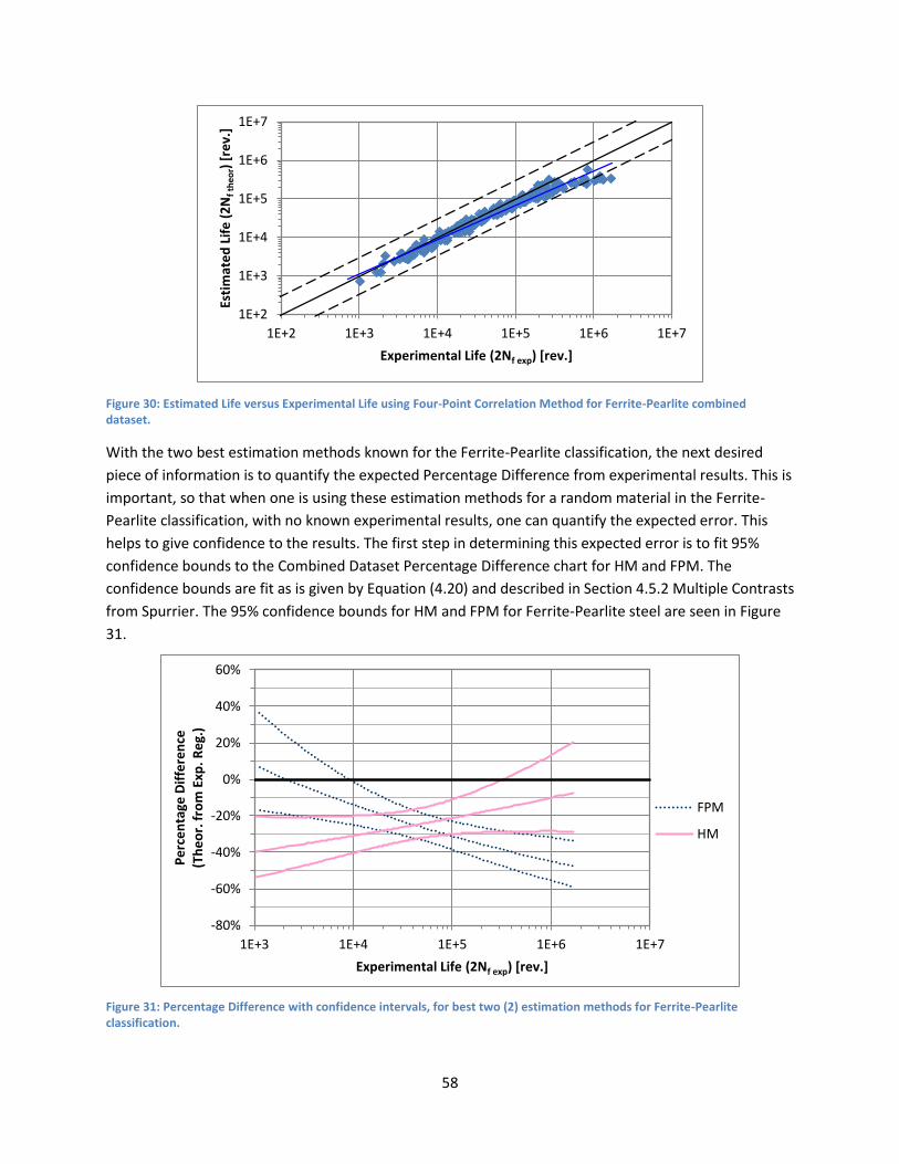
58

Figure 30: Estimated Life versus Experimental Life using Four-Point Correlation Method for Ferrite-Pearlite combined dataset.

With the two best estimation methods known for the Ferrite-Pearlite classification, the next desired

piece of information is to quantify the expected Percentage Difference from experimental results. This is

important, so that when one is using these estimation methods for a random material in the Ferrite-

Pearlite classification, with no known experimental results, one can quantify the expected error. This

helps to give confidence to the results. The first step in determining this expected error is to fit 95%

confidence bounds to the Combined Dataset Percentage Difference chart for HM and FPM. The

confidence bounds are fit as is given by Equation (4.20) and described in Section 4.5.2 Multiple Contrasts

from Spurrier. The 95% confidence bounds for HM and FPM for Ferrite-Pearlite steel are seen in Figure

31.

Figure 31: Percentage Difference with confidence intervals, for best two (2) estimation methods for Ferrite-Pearlite classification.

1E+2

1E+3

1E+4

1E+5

1E+6

1E+7

1E+2 1E+3 1E+4 1E+5 1E+6 1E+7

Esti

mat

ed

Lif

e (

2N

f th

eor)

[re

v.]


-80%

-60%

-40%

-20%

0%

20%

40%

60%

1E+3 1E+4 1E+5 1E+6 1E+7

Pe

rce

nta

ge D

iffe

ren

ce

(T

he

or.

fro

m E

xp.

Re

g.)


FPM

HM

59

The confidence bounds for the combined dataset indicate with 95% confidence where the regression

will lie for the Percentage Difference versus experimental lives. The confidence bounds do not, however,

imply that the regression for each individual material grade (from which the combined heat treatment

dataset is created) will fall within this range. The range of Percentage Difference values in which all of

the individual material grades will fall is of interest to be able to quantify the expected error. Therefore

it is of interest to compare the Percentage Difference curves for each individual material grade with the

confidence bounds, as is seen in Figure 32 for HM.

Figure 32: Comparison of all individual material grade percentage difference curves versus combined dataset 95% confidence bounds. Hardness Method, Ferrite-Pearlite classification.

From the figure it can be seen that most of the individual material grade Percentage Difference curves

fit fairly close to the 95% confidence interval from the combined dataset. There are three (3) materials

that do not fit very well within the confidence interval because they have a negative slope compared to

positive for the majority of the material grades and the confidence interval. Given that three (3) out of

ten (10) materials do not fit within the confidence interval, than the confidence intervals on their own

are insufficient to describe the expected error. However, if the highest and lowest values from the

confidence bounds are used as constant limits for the expected error, than the vast majority of the

individual material grades would fall within this range. These limits are seen in Figure 33. The limits are

rounded to the nearest 5th percentile. The upper bound is +20% and the lower bound is -55% Difference.

As can be seen from the figure, nearly all of the individual material grade Percentage Difference curves

fit within these bounds.

Therefore, for Ferrite-Pearlite steel using HM, for any material grade in this classification, the expected

Percentage Difference for an estimated life is -26% and the bounds are at +20% and -55%.

-100%

-50%

0%

50%

100%

1E+3 1E+4 1E+5 1E+6 1E+7

Pe

rce

nta

ge D

iffe

ren

ce

(Th

eo

r. f

rom

Exp

. R

eg.

)


Comb. HT. 95% Confidence

Indiv. Mat.

60

Figure 33: Constant bounds for expected error, derived from confidence interval, Hardness Method for Ferrite-Pearlite.

Similar to the above analysis for HM, the Percentage Difference curves for each individual material

grade with the confidence bounds, is seen in Figure 34 for FPM. Again there are a few individual

material grades which are outside the 95% confidence interval form the combined dataset. Therefore

the highest and lowest values from the confidence intervals are taken as constant bounds. The upper

bound is +45% and the lower bound is -65% Difference. As can be seen from the figure, nearly all of the

individual material grade Percentage Difference curves fit within these bounds.

Therefore, for Ferrite-Pearlite steel using FPM, for any material grade in this classification, the expected

Percentage Difference for an estimated life is -29% and the bounds are at +40% and -60%. This is a fairly

large bound, due to the fact that FPM does not estimate the M-C parameters as accurately as HM.

Figure 34: Comparison of all individual material grade percentage difference curves versus combined dataset 95% confidence bounds and constant bounds for expected error, Four-Point Correlation Method, Ferrite-Pearlite Steel.

-100%

-50%

0%

50%

100%

1E+3 1E+4 1E+5 1E+6 1E+7

Pe

rce

nta

ge D

iffe

ren

ce

(Th

eo

r. f

rom

Exp

. R

eg.

)


Comb. HT. 95% Confidence Indiv. Mat.

Bounds

-100%

-50%

0%

50%

100%

1E+3 1E+4 1E+5 1E+6 1E+7

Pe

rce

nta

ge D

iffe

ren

ce

(T

he

or.

fro

m E

xp.

Re

g.)



Indiv. Mat.

Bounds

61

5.1.1. Manson-Coffin Parameters from Estimated and Measured Hardness

As is discussed in Section 4.1.1 Hardness from Ultimate Tensile Strength, the hardness can be estimated

from ultimate tensile strength. Additionally, it is shown that this gives fairly accurate approximations of

the hardness. However, it is also necessary to ensure that the M-C parameters estimated by HM, using

these estimated hardness values, lead to good life estimations.

This is done by comparing the results for the each of the ten (10) different materials in the Ferrite-

Pearlite classification. The results for the measured hardness are the same as the previous section. The

results for the estimated hardness value are calculated in the same way; just the estimated hardness

value is used to calculate the M-C parameters. In Table 9, the comparison can be seen, with the

Individual Average Percentage Difference values shown. The results show that generally there is no

significant difference. Additionally, the Average of Individual Difference values from the two different

hardness values are nearly identical. Given the other sources of error and uncertainty, as noted by the

error bands seen in Figure 33, this difference is insignificant.

Therefore it is concluded that if hardness is unavailable and HM will give the best estimation results,

then the hardness can be estimated from the ultimate tensile strength. This will not result in any

significant change to the results or the expected error.

Table 9: Comparison of results by Hardness Method using measured and estimated hardness for all materials in Ferrite-Pearlite classification.

Avg. Indiv. Diff.

Mat. 1 Mat. 2 Mat. 3 Mat. 4 Mat. 5 Mat. 6 Mat. 7 Mat. 8 Mat. 9 Mat. 10

Avg. Diff. - Measured HB

25.6% 20.3% 7.6% 14.2% 30.7% 28.3% 34.6% 36.3% 32.8% 14.3% 37.1%

Avg. Diff. - Estimated HB

26.7% 28.5% 5.0% 14.1% 28.8% 27.6% 30.6% 36.6% 31.1% 24.1% 40.3%

5.2. Incomplete Hardened Steel

The summary of the results for the Incomplete Hardened classification is seen in Table 10. The meanings

of the values in the table have been described in the previous section. The Average of Individual

Difference and the Average Rank of the Individual Difference are the two most important indications of

the method giving the best results. The Combined Dataset Average Difference value is used to judge

whether the methods are consistent in giving good results, along with the Estimated Life versus

Experimental Life charts. Additionally, the combined dataset Percentage Difference chart, seen in Figure

35, is used to determine if the estimations methods are conservative, non-conservative or some

combination. From looking at the results, FPM appears to be giving the best results, followed by HM.

Both methods are predominately conservative, with FPM becoming non-conservative at higher lives.

However, for FPM due to its high Average of Individual Difference values compared to HM, it appears

that for at least one of the material grades must be giving a poor result. The consistency of the

estimation methods is first examined by looking at the combined Estimated Life versus Experimental Life

charts seen in Figure 36 and Figure 37 for FPM and HM respectively. Indeed for FPM, there appears to

62

be a lack of consistency for the method. There is a group of points which do not fit the general trend and

are significantly non-conservative estimations. This supports the observation that there appears to be

one material grade for which FPM does a poor job estimating the M-C parameters. For HM the results

are fairly consistent, with a group of points not fitting the general trend too well, but most results

remain conservative. Therefore HM appears to be a better estimation method for Incomplete Hardened

steel.

The individual material grade results will be compared versus the overall heat treatment classification

trend and error bounds will be determined as is done with the previous heat treatment.

Table 10: Summary of Average Percentage Difference values for Incomplete Hardened steel.


Avg. of Indiv. Diff. 53.1% 58.5% 55.4% 53.0% 196% 68.9% 76.3% 46.6%


Comb. Dataset Avg. Diff. 15.9% 30.7% 54.9% 36.3% 153% 17.4% 28.1% 41.7%



Figure 35: Percentage Difference for all estimation methods, for Incomplete Hardened combined dataset.

-100%

-50%

0%

50%

100%

1E+3 1E+4 1E+5 1E+6 1E+7

Pe

rce

nta

ge D

iffe

ren

ce

(Th

eo

r. f

rom

Exp

. R

eg.

)


FPM

MFPM

USM

MUSM

MM

MedM

UML

HM

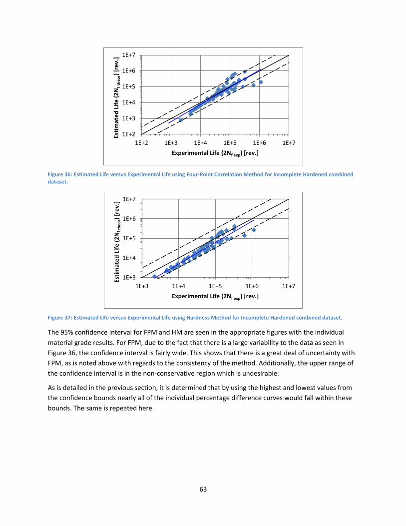
63

Figure 36: Estimated Life versus Experimental Life using Four-Point Correlation Method for Incomplete Hardened combined dataset.

Figure 37: Estimated Life versus Experimental Life using Hardness Method for Incomplete Hardened combined dataset.

The 95% confidence interval for FPM and HM are seen in the appropriate figures with the individual

material grade results. For FPM, due to the fact that there is a large variability to the data as seen in

Figure 36, the confidence interval is fairly wide. This shows that there is a great deal of uncertainty with

FPM, as is noted above with regards to the consistency of the method. Additionally, the upper range of

the confidence interval is in the non-conservative region which is undesirable.

As is detailed in the previous section, it is determined that by using the highest and lowest values from

the confidence bounds nearly all of the individual percentage difference curves would fall within these

bounds. The same is repeated here.

1E+2

1E+3

1E+4

1E+5

1E+6

1E+7

1E+2 1E+3 1E+4 1E+5 1E+6 1E+7

Esti

mat

ed

Lif

e (

2N

f th

eor)

[re

v.]


1E+3

1E+4

1E+5

1E+6

1E+7

1E+3 1E+4 1E+5 1E+6 1E+7

Esti

mat

ed

Lif

e (

2N

f th

eor)

[re

v.]


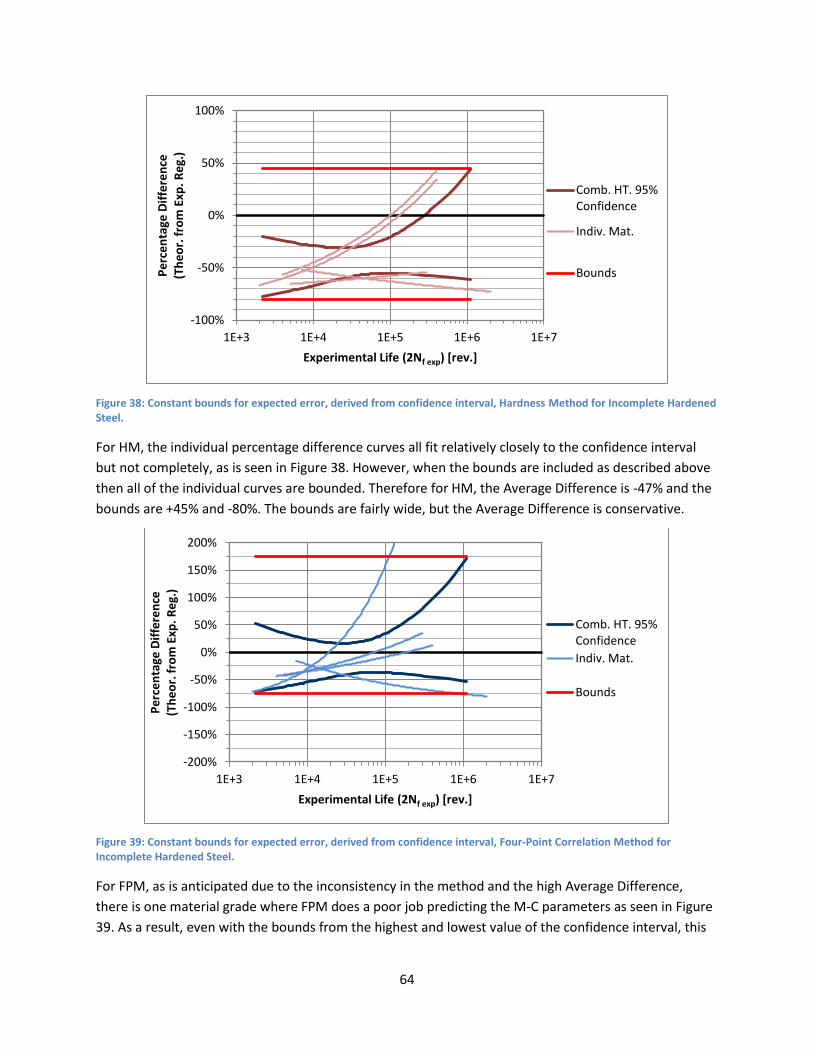
64

Figure 38: Constant bounds for expected error, derived from confidence interval, Hardness Method for Incomplete Hardened Steel.

For HM, the individual percentage difference curves all fit relatively closely to the confidence interval

but not completely, as is seen in Figure 38. However, when the bounds are included as described above

then all of the individual curves are bounded. Therefore for HM, the Average Difference is -47% and the

bounds are +45% and -80%. The bounds are fairly wide, but the Average Difference is conservative.

Figure 39: Constant bounds for expected error, derived from confidence interval, Four-Point Correlation Method for Incomplete Hardened Steel.

For FPM, as is anticipated due to the inconsistency in the method and the high Average Difference,

there is one material grade where FPM does a poor job predicting the M-C parameters as seen in Figure

39. As a result, even with the bounds from the highest and lowest value of the confidence interval, this

-100%

-50%

0%

50%

100%

1E+3 1E+4 1E+5 1E+6 1E+7

Pe

rce

nta

ge D

iffe

ren

ce

(T

he

or.

fro

m E

xp.

Re

g.)



Indiv. Mat.

Bounds

-200%

-150%

-100%

-50%

0%

50%

100%

150%

200%

1E+3 1E+4 1E+5 1E+6 1E+7

Pe

rce

nta

ge D

iffe

ren

ce

(T

he

or.

fro

m E

xp.

Re

g.)



Indiv. Mat.

Bounds

65

material is not bounded. Therefore, caution is advised with this method. The bounds are +175% and -

75%. The Average Difference is not accurate due to the inconsistency of the method.

5.3. Martensite-Lightly Tempered Steel

The summary of the results for the Martensite-Lightly Tempered classification is seen in Table 11. The

combined dataset Percentage Difference chart is seen in Figure 40. From looking at the results, MUSM

and MFPM appear to be giving the best results. MFPM is on average conservative, while MUSM is

slightly on the non-conservative side. The number of life estimations that are conservative and non-

conservative can be checked by looking at the combined datset Estimated Life versus Experimental life

charts, seen in Figure 45 and Figure 46 for MFPM and MUSM respectively.

Table 11: Summary of Percentage Difference values for Martensite-Lightly Tempered steel.


Avg. of Indiv. Diff. 39.1% 32.8% 106% 50.1% 2025% 323% 380% 55.7%


Comb. Dataset Avg. Diff. 6.9% 12.0% 83.2% 21.9% 1314% 262% 287% 57.7%



Figure 40: Percentage Difference for all estimation methods, for Martensite-Lightly Tempered combined dataset.

Figure 41 and Figure 42 show the individual percentage difference curves with the combined dataset

confidence interval for MFPM and MUSM respectively. For both methods it can be seen that there is

one individual material grade for which both methods poorly estimate the M-C parameters and

therefore the lives. This particular material is examined to determine if there are any specific

characteristics which result in a poor estimation being achieved. The material in question has two

related characteristics that may be leading to poor estimations. This material has 2297UTS MPa and

-100%

-50%

0%

50%

100%

150%

200%

250%

300%

1E+2 1E+3 1E+4 1E+5 1E+6 1E+7

Pe

rce

nta

ge D

iffe

ren

ce

(T

he

or.

fro

m E

xp.

Re

g.)


FPM

MFPM

USM

MUSM

MM

MedM

UML

HM

66

an experimental regression fatigue strength coefficient of ' 4850f MPa . Both of these values are

approximately 15% higher than any other material grades in this research. This is a very high value for

UTS and therefore it is outside the typical range for which these estimation methods have been

validated. This can be seen particularly for Uniform Material Law (UML). For UML, 'f is calculated to be

a negative value, due to the very high UTS

E

. As is noted in the literature review, Section 3.10 Uniform

Material Law (UML) by Bäumel and Seeger , Meggiolaro [21] noted that for steels, σUTS must be less than

~2.2 GPa (with typical values of E), otherwise negative values of εf’ will occur. This is the case for this

material.

Therefore, the conclusion is that for materials with very high UTS values, poor estimations may occur

and the use of estimation methods is not recommended.

Figure 41: Confidence interval and individual material grade results for Modified Four-Point Correlation Method for Martensite-Lightly Tempered Steel.

-150%

-100%

-50%

0%

50%

100%

150%

1E+2 1E+3 1E+4 1E+5 1E+6 1E+7

Pe

rce

nta

ge D

iffe

ren

ce

(Th

eo

r. f

rom

Exp

. R

eg.

)



Indiv. Mat.

67

Figure 42: Confidence interval and individual material grade results for Modified Universal Slopes Method for Martensite-Lightly Tempered Steel.

The one poor material cause the confidence bands to be much larger than would be necessary and so all

of the results are recalculated ignoring this material. The new results are shown below.

Table 12: Summary of Percentage Difference values, with poor material grade removed. Martensite-Lightly Tempered Steel.


Avg. of Indiv. Diff. 23.5% 28.6% 88.7% 29.5% 737% 196% 121% 57.0%


Comb. Dataset Avg. Diff. 23.4% 22.7% 75.8% 3.8% 621% 165% 129% 60.0%



Figure 43: Percentage Difference for all estimation methods, for Martensite-Lightly Tempered combined dataset with removed material grade.

-100%

-50%

0%

50%

100%

150%

200%

250%

1E+2 1E+3 1E+4 1E+5 1E+6 1E+7

Pe

rce

nta

ge D

iffe

ren

ce

(Th

eo

r. f

rom

Exp

. R

eg.

)



Indiv. Mat.

-100%

-50%

0%

50%

100%

150%

200%

250%

300%

1E+2 1E+3 1E+4 1E+5 1E+6 1E+7

Pe

rce

nta

ge D

iffe

ren

ce

(T

he

or.

fro

m E

xp.

Re

g.)


FPM

MFPM

USM

MUSM

MM

MedM

UML

HM

68

From Table 12, it can be seen that FPM, MFPM and MUSM give the best results for this heat treatment

classification, with these methods giving the best average results for each of the individual material

grades. The consistency of each of these estimation methods is examined by looking at the combined

Estimated Life versus Experimental Life charts seen in Figure 44, Figure 45 and Figure 46 for FPM, MFPM

and MUSM respectively. From looking at all of these figures, there is a lot of variability to the data and

therefore inconsistency to the data. However, this variability is mostly related to the experimental data,

as the Experimental Regression Life versus Experimental Life plot also shows a fair amount of variability

as seen in Figure 47. Therefore, determination of the best and most consistent of these estimation

methods cannot be extracted from these plots and so the individual material grade results are

compared with the 95% confidence bands, as has been previously done.

Figure 44: Estimated Life versus Experimental Life using Four-Point Correlation Method for Martensite-Lightly Tempered combined dataset.

Figure 45: Estimated Life versus Experimental Life using Modified Four-Point Correlation Method for Martensite-Lightly Tempered combined dataset.

1E+2

1E+3

1E+4

1E+5

1E+6

1E+7

1E+2 1E+3 1E+4 1E+5 1E+6 1E+7

Esti

mat

ed

Lif

e (

2N

f th

eor)

[re

v.]


1E+2

1E+3

1E+4

1E+5

1E+6

1E+7

1E+2 1E+3 1E+4 1E+5 1E+6 1E+7

Esti

mat

ed

Lif

e (

2N

f th

eor)

[re

v.]


69

Figure 46: Estimated Life versus Experimental Life using Modified Universal Slope Method for Martensite-Lightly Tempered combined dataset.

Figure 47: Experimental Regression Life versus Experimental Life for Martensite-Lightly Tempered combined dataset.

Figure 48: Confidence interval and individual material grade results for Four-Point Correlation Method for Martensite-Lightly Tempered steel, with removed material grade.

1E+2

1E+3

1E+4

1E+5

1E+6

1E+7

1E+2 1E+3 1E+4 1E+5 1E+6 1E+7 Esti

mat

ed

Lif

e (

2N

f th

eor)

[re

v.]


1E+2

1E+3

1E+4

1E+5

1E+6

1E+2 1E+3 1E+4 1E+5 1E+6

Exp

eri

me

nta

l Re

gre

ssio

n L

ife

(2

Nf

exp

re

g) [

rev.

]


-100%

-50%

0%

50%

100%

150%

200%

1E+2 1E+3 1E+4 1E+5 1E+6 1E+7

Pe

rce

nta

ge D

iffe

ren

ce

(Th

eo

r. f

rom

Exp

. R

eg.

)



Indiv. Mat.

70

Figure 49: Confidence interval and individual material grade results for Modified Four-Point Correlation Method for Martensite-Lightly Tempered steel, with removed material grade.

Figure 50: Confidence interval and individual material grade results for Modified Universal Slopes Method for Martensite-Lightly Tempered steel, with removed material grade.

From comparing Figure 48, Figure 49 and Figure 50, it can be seen that while FPM has the lowest

Average Percentage Difference value, as seen in Table 12, on the individual material grade results it is

inconsistent. This inconsistency leads to it having a very wide 95% confidence interval. Therefore MFPM

and then MUSM are the best estimation methods for Martensite-Lightly Tempered steel. The bounds on

the range for the individual estimations are +85% and -80% for MFPM as seen in Figure 49, with an

Average Percentage Difference of +/-29% and +155% and -70% for MUSM, with an Average Percentage

Difference of +/-30%. Therefore MFPM is the better method as its results are generally conservative

and more consistent.

-100%

-50%

0%

50%

100%

1E+2 1E+3 1E+4 1E+5 1E+6 1E+7

Pe

rce

nta

ge D

iffe

ren

ce

(T

he

or.

fro

m E

xp.

Re

g.)



Indiv. Mat.

Bounds

-100%

-50%

0%

50%

100%

150%

200%

1E+2 1E+3 1E+4 1E+5 1E+6 1E+7

Pe

rce

nta

ge D

iffe

ren

ce

(Th

eo

r. f

rom

Exp

. R

eg.

)



Indiv. Mat.

Bounds

71

The 95% confidence interval for MFPM and MUSM are seen in Figure 49 and Figure 50. For MUSM, due

to the fact that there is a large variability to the data as seen in Figure 46, the confidence interval is fairly

wide. This shows that there is a great deal of uncertainty with MUSM, as is noted above with regards to

the consistency of the method.

5.4. Martensite-Tempered Steel

The summary of the results for the Martensite-Tempered classification is seen in Table 13. As can be

seen, while UML has the lowest Average Rank of Individual Difference values, it is found that MFPM and

MUSM have the lowest Average of Individual Difference values and therefore are the better estimation

methods for this heat treatment classification. Additionally, as can be seen in Figure 52 for Uniform

Material Law compared to Figure 53 and Figure 54 for MUSM and MFPM respectively, UML is a less

consistent method, as there is more variability in the results given that the same experimental data is

used. The Percentage Difference chart, seen in Figure 51, is used to determine if the estimations

methods are conservative, non-conservative of some combination. MUSM and MFPM are

predominately conservative.

The individual material grade results will be compared versus the overall classification trend and error

bounds will be determined as with the previous heat treatment classifications.

Table 13: Summary of Percentage Difference values for Martensite-Tempered Steel.


Avg. of Indiv. Diff. 39.0% 33.2% 49.8% 33.7% 182% 49.3% 35.9% 47.3%


Comb. Dataset Avg. Diff. 50.1% 34.9% 62.0% 36.2% 103% 35.9% 19.7% 49.3%



Figure 51: Percentage Difference for all estimation methods, for Martensite-Tempered combined dataset.

-100%

-50%

0%

50%

100%

150%

200%

1E+3 1E+4 1E+5 1E+6 1E+7

Pe

rce

nta

ge D

iffe

ren

ce

(Th

eo

r. f

rom

Exp

. R

eg.

)


FPM

MFPM

USM

MUSM

MM

MedM

UML

HM

72

Figure 52: Estimated Life versus Experimental Life using Uniform Material Law for Martensite-Tempered combined dataset.

Figure 53: Estimated Life versus Experimental Life using Modified Universal Slopes Method for Martensite-Tempered combined dataset.

Figure 54: Estimated Life versus Experimental Life using Modified Four-Point Correlation Method for Martensite- Tempered combined dataset.

1E+2

1E+3

1E+4

1E+5

1E+6

1E+7

1E+2 1E+3 1E+4 1E+5 1E+6 1E+7 Esti

mat

ed

Lif

e (

2N

f th

eor)

[re

v.]


1E+2

1E+3

1E+4

1E+5

1E+6

1E+7

1E+2 1E+3 1E+4 1E+5 1E+6 1E+7 Esti

mat

ed

Lif

e (

2N

f th

eor)

[re

v.]


1E+2

1E+3

1E+4

1E+5

1E+6

1E+7

1E+2 1E+3 1E+4 1E+5 1E+6 1E+7 Esti

mat

ed

Lif

e (

2N

f th

eor)

[re

v.]


73

The individual material grade results are compared versus the 95% confidence bands for the combined

dataset for MUSM in Figure 55. As can be seen, the method is fairly consistent and nearly all of the

results are conservative or partially conservative. The error bounds are fit at +65% and -75% as has been

done in previous sections. The Average Difference value is -34% as shown in Table 13.

Figure 55: Constant bounds for expected error, derived from confidence interval, Modified Universal Slopes Method for Martensite-Tempered Steel.

For MFPM, there is more of a slope to the results and so the bounds are wider at +100% and -80%. The

method is predominately conservative as well. The Average Difference value is -33% as shown in Table

13.

Figure 56: Constant bounds for expected error, derived from confidence interval, Modified Four-Point Correlation Method for Martensite-Tempered Steel.

-100%

-50%

0%

50%

100%

1E+3 1E+4 1E+5 1E+6 1E+7

Pe

rce

nta

ge D

iffe

ren

ce

(Th

eo

r. f

rom

Exp

. R

eg.

)



Indiv. Mat.

Bounds

-100%

-50%

0%

50%

100%

1E+3 1E+4 1E+5 1E+6 1E+7

Pe

rce

nta

ge D

iffe

ren

ce

(T

he

or.

fro

m E

xp.

Re

g.)



Indiv. Mat.

Bounds

74

5.5. Micro-Alloyed Steel

The summary of the results for the Micro-Alloyed Steel classification is seen in Table 14, and the

Percentage Difference chart is seen in Figure 57. From looking at these, only USM gives consistently

good and conservative results. MedM gives the next best results, but they are on average non-

conservative. The Estimated Life versus Experimental Life charts, seen in Figure 58 and Figure 59 for

USM and MedM respectively can be used to determine whether the estimated lives are conservative

and non-conservative for each data point. USM is almost entirely conservative while MedM is a mix of

conservative and non-conservative. Therefore, only USM is a recommended estimation method for this

material, as others will give non-conservative and inconsistent results.

Table 14: Summary of Percentage Difference values for Micro-Alloyed Steel.


Avg. of Indiv. Diff. 82.6% 56.2% 18.2% 36.6% 99.9% 36.3% 76.8% 41.9%





Figure 57: Percentage Difference for all estimation methods, for Micro-Alloyed combined dataset.

-50%

0%

50%

100%

1E+2 1E+3 1E+4 1E+5 1E+6

Pe

rce

nta

ge D

iffe

ren

ce

(T

he

or.

fro

m E

xp.

Re

g.)


FPM

MFPM

USM

MUSM

MM

MedM

UML

HM

75

Figure 58: Estimated Life versus Experimental Life using Universal Slope Method for Micro-Alloyed combined dataset.

Figure 59: Estimated Life versus Experimental Life using Medians Method for Micro-Alloyed combined dataset.

The individual material grade curves are compared versus the combined dataset 95% confidence

bounds. As can be seen in Figure 60, the individual results match very closely with the overall trend,

which is expected given the consistency to the estimated lives seen in Figure 58. The bounds are still

calculated the same as originally described, with the bounds being set at +45% and -50%. The Average

Percentage Difference is -18%.

1E+2

1E+3

1E+4

1E+5

1E+6

1E+2 1E+3 1E+4 1E+5 1E+6

Esti

mat

ed

Lif

e (

2N

f th

eor)

[re

v.]


1E+2

1E+3

1E+4

1E+5

1E+6

1E+2 1E+3 1E+4 1E+5 1E+6 Esti

mat

ed

Lif

e (

2N

f th

eor)

[re

v.]


76

Figure 60: Constant bounds for expected error, derived from confidence interval, Universal Slopes Method for Micro-Alloyed Steel.

As will be explained in Section 7.5 Micro-Alloyed Steel, MedM will also be examined. The Average

Percentage Difference is +36% and the bounds are +95% and -35%. The method is somewhat

inconsistent as can be seen in Figure 61, as the individual material grade Percentage Difference curves

are varied. This can also be seen from the results in Figure 59.

Figure 61: Constant bounds for expected error, derived from confidence interval, Medians Method for Micro-Alloyed Steel.

-50%

0%

50%

1E+3 1E+4 1E+5 1E+6

Pe

rce

nta

ge D

iffe

ren

ce

(T

he

or.

fro

m E

xp.

Re

g.)



Indiv. Mat.

Bounds

-100%

-50%

0%

50%

100%

1E+3 1E+4 1E+5 1E+6

Pe

rce

nta

ge D

iffe

ren

ce

(T

he

or.

fro

m E

xp.

Re

g.)



Indiv. Mat.

Bounds

77

5.6. Carburized Steel

The results for the Carburized Steel classification, seen in Figure 62 and Table 15 show that most of the

estimation methods are quite conservative. The estimation methods that give the best results are

MedM and UML. The consistency and level of conservatism for these methods can be assessed from

Figure 63 and Figure 64 for MedM and UML respectively. MedM gives entirely conservative and

consistent estimations and this is shown from the near constant Percentage Difference slope in Figure

62. For UML, the method is conservative, but overly conservative in some cases and it is inconsistent

with a large change in the level of conservatism depending on the life range. Therefore, this method is

not as good as MedM but is still conservative.

Table 15: Summary of Percentage Difference values for Carburized Steel.


Avg. of Indiv. Diff. 59.3% 65.4% 88.8% 79.4% 87.3% 44.1% 51.0% 254%


Comb. Dataset Avg. Diff. 54.9% 60.2% 88.5% 78.6% 120% 44.3% 48.9% 369%



Figure 62: Percentage Difference for all estimation methods, for Carburized combined dataset.

-100%

-50%

0%

50%

100%

1E+3 1E+4 1E+5 1E+6 1E+7

Pe

rce

nta

ge D

iffe

ren

ce

(Th

eo

r. f

rom

Exp

. R

eg.

)


FPM

MFPM

USM

MUSM

MM

MedM

UML

HM

78

Figure 63: Estimated Life versus Experimental Life using Medians Method for Carburized combined dataset.

Figure 64: Estimated Life versus Experimental Life using Uniform Material Law for Carburized combined dataset.

The individual material grade curves are compared versus the combined dataset 95% confidence

interval. As can be seen in Figure 65 and Figure 66, for MedM and UML respectively, the individual

results match very closely with the overall trend. This is expected for MedM given the consistency to the

estimated lives seen in Figure 63. For UML it shows that the results amongst individual material grades

are consistent, but the estimation method just gives changing levels of conservatism depending on the

life range. The bounds for MedM are +10% and -70%. The Average Percentage Difference is -44%. For

UML, the bounds are +80% and -85%. The large bounds are due to the large changes in conservatism

over the life range. The Average Percentage Difference is -51%.

1E+3

1E+4

1E+5

1E+6

1E+7

1E+3 1E+4 1E+5 1E+6 1E+7

Esti

mat

ed

Lif

e (

2N

f th

eor)

[re

v.]


1E+3

1E+4

1E+5

1E+6

1E+7

1E+3 1E+4 1E+5 1E+6 1E+7

Esti

mat

ed

Lif

e (

2N

f th

eor)

[re

v.]


79

Figure 65: Constant bounds for expected error, derived from confidence interval, Medians Method for Carburized Steel.

Figure 66: Constant bounds for expected error, derived from confidence interval, Uniform Material Law for Carburized Steel.

5.7. Austempered Steel

The results for the Austempered Steel classification are seen in Table 16 and Figure 67. As can be seen,

all of the methods give very non-conservative estimations. Therefore, there is no estimation method

that gives good estimations for this heat treatment classification. The reasons for these poor estimations

can be partially explained by some of the characteristics of Austempered Steel. The heat treatment

characteristics have been detailed briefly in Section 2.2.1 Austempered Steel. From this section, it is

noted that bainite is the primary component in Austempered Steel, compared to the pearlite and

martensite with the other heat treatments. It is beyond the scope of this project that look at how these

different microstructural arrangements affects the estimation method. However, for Austempered

-100%

-50%

0%

50%

100%

1E+3 1E+4 1E+5 1E+6 1E+7

Pe

rce

nta

ge D

iffe

ren

ce

(Th

eo

r. f

rom

Exp

. R

eg.

)



Bounds

-100%

-50%

0%

50%

100%

1E+3 1E+4 1E+5 1E+6 1E+7

Pe

rce

nta

ge D

iffe

ren

ce

(T

he

or.

fro

m E

xp.

Re

g.)



Indiv. Mat.

Bounds

80

Steel, the changes to material properties as a result of these microstructural differences can be used to

explain the poor estimations. The elastic modulus for the three Austempered Steels ranges from 163 to

170 GPa. By comparison, the rest of the heat treatment classifications that have been looked at range

from 190 to 217 GPa. This is a significant difference, which may help to explain the poor estimation for

austempered steel. Additionally, most of the estimation methods have been developed from steel with

much higher elastic modulus. For example, the range of elastic modulus is 203 to 227 GPa for HM [24],

180 to 220 GPa for MUSM [23] with only 1 material at the 180 GPa range and the median elastic

modulus for the 724 steels in the development of MedM is 205 GPa [21]. Therefore these Austempered

Steels, with low elastic modulus do not fit the characteristics of the materials used to develop the

estimation methods, leading to poor estimations.

Table 16: Summary of Percentage Difference values for Austempered Steel.


Avg. of Indiv. Diff. 905% 1437% 125% 624% 42328% 1318% 2172% 629%


Comb. Dataset Avg. Diff. 604% 826% 65.5% 398% 9215% 782% 1131% 485%



Figure 67: Percentage Difference for all estimation methods, for Austempered combined dataset.

Additionally, it can be seen from the Experimental Regression Life versus Experimental Life plot in Figure

68 that the experimental data is inconsistent, meaning that making good estimations is difficult.

-100%

-50%

0%

50%

100%

150%

200%

250%

300%

350%

400%

1E+2 1E+3 1E+4 1E+5 1E+6 1E+7

Pe

rce

nta

ge D

iffe

ren

ce

(Th

eo

r. f

rom

Exp

. R

eg.

)


FPM

MFPM

USM

MUSM

MM

MedM

UML

HM

81

Figure 68: Experimental Regression Life versus Experimental Life for Austempered combined dataset.

5.8. General Steel Classification

All of the previous results have focused on determining the best estimation method for each heat

treatment classification. However, the heat treatment for a particular material specimen may not be

known but its monotonic properties are available. In this case, it would very unclear as to which

estimation method to use from the previous assessments. Additionally, if one material is undergoing a

heat treatment process, changing its heat treatment from one classification to another, it may be

prudent to use the same estimation method for consistency of the results, in both heat treatment

states. For both of these situations, it would be beneficial to know, in general terms which estimation

method is the best, regardless of heat treatment.

To do this, all of the results across every heat treatment classification will be combined into one set and

analyzed to determine which estimation method gives the best results overall. This is done through

taking all of the individual Average Percentage Difference values for each material grade and for each

estimation method.

The first step in determining the best estimation method is to determine if there is any correlation

between the individual Average Percentage Difference values and any other characteristics of the

material. If any sort of correlation existed, it would help to provide reasoning for the difference in the

best estimation method between the heat treatment classifications. The characteristics of the material

that are compared are the monotonic properties data: E , UTS and HB . An example of these

comparisons for HM is seen in Figure 69.

1E+3

1E+4

1E+5

1E+6

1E+7

1E+3 1E+4 1E+5 1E+6 1E+7

Exp

eri

me

nta

l Re

gre

ssio

n L

ife

(2

Nf

exp

re

g) [

rev.

]


82

Figure 69: Individual Average Percentage Difference versus monotonic properties for Hardness Method, all heat treatment classifications: a) Elastic Modulus, b) Ultimate Tensile Strength, c) Brinell Hardness

From looking at Figure 69, it appears that there is some sort of an influence on the Average Percentage

Difference based on UTS and HB , but most predominately HB . Additionally, looking at these curves for

the other seven (7) estimation methods, there also seems to be a slight relationship between which

estimation method gives the best result depending on the hardness range. There is no statistically

0%

50%

100%

150%

200%

250%

300%

350%

185000 190000 195000 200000 205000 210000 215000 220000 Ave

rage

Pe

rce

nta

ge D

iffe

ren

ce

E [MPa]

0%

50%

100%

150%

200%

250%

300%

350%

250 500 750 1000 1250 1500 1750 2000 Ave

rage

Pe

rce

nta

ge D

iffe

ren

ce

σUTS [MPa]

0%

50%

100%

150%

200%

250%

300%

350%

0 100 200 300 400 500 600 700 800 Ave

rage

Pe

rce

nta

ge D

iffe

ren

ce

Hardness [HB]

83

significant correlation to show a direct relationship between any of the monotonic properties and how

accurate the estimation method will be.

Therefore, the results for each estimation method are plotted versus the hardness, grouped by

estimation method. This is seen in Figure 70. This means that for each material grade, there is a point for

each estimation method; therefore eight (8) in total. In the figure, the Average Percentage Difference

has been restricted to 350% and so four (4) points from MM which exceed this value are not shown.

Figure 70: Average Percentage Difference versus hardness for all estimation methods.

From this figure, the results can be confused within the very large number of points; however looking

closely a few observations can be made.

The data points at the high hardness range correspond to the material grades for Carburized

Steel and as is seen in Section 5.6 Carburized Steel, these estimations are not as good due to the

type of heat treatment. Therefore, not too much should be read into these points and they are

removed from the analysis presented further down in this section.

If one looks closely at the figure to see where the points for each estimation method lie in

comparison to the other estimation methods, it can be seen that there are some interesting

differences. Particularly, if one follows the results for some of the particular estimation methods

versus the hardness, it can be seen that certain estimation methods give better results in certain

ranges of hardness.

It is found that HM gives the best results below 300 HB and above 300 HB, MFPM and MUSM give

better results. Table 17 shows the average of the Average Percentage Difference values across all of

the material grades for each estimation method, with the material grades separated at 300 HB. As

can be seen, for hardness less than 300 HB HM gives significantly better results on average than the

other estimation method. This observation can also be verified by examining HM versus the rest of

0%

50%

100%

150%

200%

250%

300%

350%

0 100 200 300 400 500 600 700 800

Ave

rage

Pe

rce

nta

ge D

iffe

ren

ce

Hardness [HB]

FPM

MFPM

USM

MUSM

MM

MedM

UML

HM

84

the estimation methods for each individual material grade, which is seen in Figure 71. In this figure it

can be seen that HM is consistently giving the best or close to one of the best estimations for the

material grades in this hardness range.

Table 17: Average of the Average Percentage Difference values across all material grades, for each estimation method by hardness range.

Hardness [HB] Number of

Material Grades FPM MFPM USM MUSM MM MedM UML HM

<300 19 42.8% 43.6% 41.8% 38.8% 62.4% 54.1% 46.8% 32.4%

>300 8 40.1% 41.8% 67.9% 38.9% 459.0% 118.0% 90.4% 56.3%

Figure 71: Average Percentage Difference versus hardness (<300 HB) for individual material grades. Comparison of Hardness Method to all other estimation methods.

For the hardness range greater than 300 HB, it can be seen from Table 17 that HM no longer gives close

to the best estimations. From the table, it can be seen that MUSM followed by FPM and MFPM give the

best results for hardness greater than 300 HB. Even though FPM gives the second best results, it is

ignored because its results are often non-conservative and inconsistent. These concerns with FPM have

been noted in the results for the Incomplete Hardened, Martensite-Lightly Tempered and Martensite-

Tempered classifications (Sections 5.2 to 5.4). These classifications contain the material grades with

hardness greater than 300 HB. Due to the inconsistency and non-conservative results, FPM is ignored.

MFPM is considered since it gives similar average results as MUSM and as can be seen in Figure 72

MUSM and MFPM alternate as to which gives the best result for a single individual result.

0%

25%

50%

75%

100%

125%

150%

50 100 150 200 250 300

Ave

rage

Pe

rce

nta

ge D

iffe

ren

ce

Hardness [HB]

HM

All Others

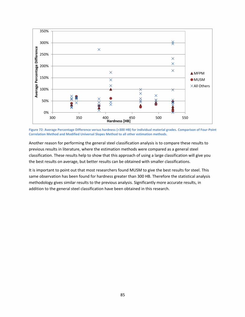
85

Figure 72: Average Percentage Difference versus hardness (>300 HB) for individual material grades. Comparison of Four-Point Correlation Method and Modified Universal Slopes Method to all other estimation methods.

Another reason for performing the general steel classification analysis is to compare these results to

previous results in literature, where the estimation methods were compared as a general steel

classification. These results help to show that this approach of using a large classification will give you

the best results on average, but better results can be obtained with smaller classifications.

It is important to point out that most researchers found MUSM to give the best results for steel. This

same observation has been found for hardness greater than 300 HB. Therefore the statistical analysis

methodology gives similar results to the previous analysis. Significantly more accurate results, in

addition to the general steel classification have been obtained in this research.

0%

50%

100%

150%

200%

250%

300%

350%

300 350 400 450 500 550

Ave

rage

Pe

rce

nta

ge D

iffe

ren

ce

Hardness [HB]

MFPM

MUSM

All Others

86

5.9. Summary Steel Heat Treatment Classifications

Table 18 shows the summary of the best estimation method for each heat treatment classification and

the general steel classification, as has been determined in the preceding sections.

Table 18: Summary of best estimation methods for each heat treatment.

Recommended

Estimation Methods

1 2

Ferrite-Pearlite Steel HM FPM

Incomplete Hardened Steel HM FPM

Martensite-Lightly Tempered Steel

MFPM MUSM

Martensite-Tempered Steel MUSM MFPM

Micro-Alloyed Steel USM MedM

Carburized Steel MedM UML

Austempered Steel Not Recommended

General Steel Classification <300 HB

HM

General Steel Classification >300 HB

MUSM MFPM

5.10. Comparison of Results from Multiple Contrasts and Goodness of

Fit Criteria.

In Section 4.5 Criterion for Comparison of Estimation Method, the multiple contrast comparison method

and the Goodness of Fit criteria by Park and Song [19] are discussed. It is noted that the Goodness of Fit

criteria is not statistically based but utilizes the concepts of the linear regression parameters to try and

determine the best estimation method. Some of the problems associated with this approach are

mentioned and these problems are illustrated in this section using some examples from the data

analyzed.

The first point that is noted with regards to the Goodness of Fit criteria is that the linear regression

parameters ( and ) are compared versus the perfect correlation values ( 1 and 0 ). However, in

practice these values are not necessarily achievable. This is because, even for experimental data it is not

guaranteed that the regression formed from the lives estimated from the experimental M-C parameters

and the experimental data would lead to a regression with 1 and 0 . This is discussed in Section

4.4 Statistical Analysis and is due to the variability in the data and the fact that real data only imperfectly

fits the M-C relationship [11]. Due to the fact that experimental data cannot guarantee a perfect

correlation, it is not prudent to expect that estimated M-C parameters could do so. It is possible that this

would occur, but it is more likely to be by chance than an indication of excellent results. It should be

noted that typically the regression of Experimental Regression Life versus Experimental Life results in a

87

near perfect correlation, but not exactly. Therefore this difference is unlikely to have a significant effect

but shows an example of the statistical basis of the problem not being fully considered.

The larger discrepancies with the statistical basis of the Goodness of Fit criteria involve the arbitrary

definitions for the criteria. As is previously mentioned, for the individual material grade analysis and

combined dataset analysis, the intercept ( ), slope ( )and correlation coefficient ( r ) are all used to

determine how ‘far’ from the perfect correlation the linear regression is. However, the measures for

how far away each term is, has been arbitrarily defined. As such, equal weighting is given to these three

terms and the combined term. All of this can be seen in Equation (4.18), which is repeated below.

1 1

1 1 1 1 1 1 11 1( )

4

N Ni i i i i

a Dset a ii i

rE E

N N

Additionally, once the average value for each individual dataset has been found using Equation (4.18)

and for the combined dataset using Equation (4.17), the number of points within a scatter band of a

factor of 3 is found using Equation (4.16). Finally, all of these three criteria are averaged using Equation

(4.15).

An example of the calculation for the Goodness of Fit criteria is shown in Table 19 for the Ferrite-Pearlite

steel classification.

Table 19: Goodness of Fit for Ferrite-Pearlite classification.


( 3)fE s 0.961 0.994 0.894 0.927 0.994 0.453 0.994 1.000

( )a TotE 0.811 0.854 0.851 0.613 0.918 0.742 0.843 0.825

( )a DsetE 0.718 0.795 0.742 0.650 0.728 0.719 0.792 0.765

E 0.830 0.881 0.829 0.730 0.880 0.638 0.877 0.863

Rank E 5 1 6 7 2 8 3 4

With the Goodness of Fit criteria calculated for the Ferrite-Pearlite classification, it is compared to the

results from the analysis done in this research using Multiple Contrast. The results have been presented

in Section 5.1 Ferrite-Pearlite Steel. The result for Goodness of Fit is compared versus the Rank of the

Average Individual Percentage Difference value, as this is the primary result used to determine the best

estimation method. This comparison is seen in Table 20. As can be seen, there are some discrepancies

between the two results. Most notably, Goodness of Fit would have MFPM as the best method; it is far

from the best from the Multiple Contrasts analysis. FPM has the opposite occur. Finally, HM which is the

best method by Multiple Contrast is only the fourth best by Goodness of Fit. Some of the results for

Goodness of Fit are quite close as can be seen from Table 19, but this is mostly due to the fact that three

different criteria are used and averaged. This means that a poor result for one portion of the criteria can

be balanced out by other good results. Particularly the percentage of data in a factor of 3 brings up

some of the E values for a number of the estimation methods.

88

Table 20: Comparison of ranking for Goodness of Fit criteria and Multiple Contrasts criteria for Ferrite-Pearlite Steel.



Rank E 5 1 6 7 2 8 3 4

Overall, these results show that Goodness of Fit provides some reasonable results and so the analyses

done by Park and Song using this criterion ( [19], [12]) provide some useful observations. However, as

has been pointed out, the criterion does not have a solid statistical basis and so it is not appropriate to

use it. Therefore Multiple Contrasts has been used, based on similar principles but with statistical basis.

89

6. Estimation of Ramberg-Osgood Parameters

6.1. Compatibility of Manson-Coffin and Ramberg-Osgood Parameters

In the typical strain-life fatigue analysis, the life for a component or structure is calculated from a given

loading or stress history. This requires that the R-O relationship be used to calculate the strain history

from the stress history and then the fatigue life from the strain history using the M-C relationship. This

has been laid out in more detail in Section 1.1 Strain-Life Method. These two relationships are required

to determine the fatigue life and therefore there are six (6) material parameters (plus elastic modulus)

required. They can all be determined from the same set of data and are in fact theoretically related to

each other. The R-O relationship (seen in Equation (6.1)) and M-C relationship (seen in Equation (6.2))

have a similar form, with both representing the total strain amplitude as the sum of the elastic and

plastic strains. The elastic and plastic portions of the strain from each equation can be equated to each

other and then the relationships between the R-O and M-C parameters can be determined.

'1

'ε ε ε

na a

a e pE K

(6.1)

'

b c'f fε ε 2N 2N

f

a e p fE

(6.2)

From equating the elastic and plastic terms in both equations, it can be fairly easily solved that:

' bn

c (6.3)

'

'

'

'n

f

f

K

(6.4)

A full derivation of these relations is thoroughly presented by Nieslony in [6]. These relationships

between the M-C parameters and the R-O parameters are called the compatibility equations and mean

that there are in fact only four (4) unknown material parameters.

However, these compatibility equations in practice are usually not satisfied exactly. This is due to the

conventional way that the M-C parameters and R-O parameters are determined. As is briefly detailed in

Section 1.1 Strain-Life Method, the conventional way to determine the M-C and R-O parameters from

experiments is through testing a number of specimens under constant strain amplitude fatigue tests.

From each specimen, the strain amplitude, fatigue life and stabilized stress amplitude is known. Given

this data from multiple specimens, M-C parameters are determined from fitting elastic and plastic strain

(calculated using the strain and stress amplitudes) versus life and the R-O parameters are determined

from fitting the stress amplitude versus plastic strain.

Therefore the same set of fatigue testing data is used to determine the M-C parameters and R-O

parameters, but this does not guarantee compatibility of the equations due to the fact that different

90

pieces of data are used. These pieces of data are not guaranteed to be in agreement. Additionally, the

way that the M-C and R-O parameters are fit separately, means that they are treated as separate

experimental results [6]. Some inherent experimental error and the fact that some materials take time

to reach a stabilized hysteresis loop cause some of the incompatibility.

To overcome the fact that the M-C and R-O parameters are fit separately but using the same data and

thus compatibility is not ensured, Nieslony [6] proposes to plot the three sets of experimental data

(strain, stress, life) in 3-D space and fit one line through the data. Then by projecting this line onto the

plane for strain versus life, the M-C parameters can be determined and projecting it on the stress versus

strain plane allows the R-O parameters to be determined. Since the data for the M-C and R-O

parameters are fit using one line, compatibility of the equations is ensured.

While this method of fitting the M-C and R-O parameters to ensure compatibility appears to be a good

approach and eliminates the compatibility problem, the more important implication for this research is

to determine how fitting the conventional manner affects the results. This is because in using the

estimation methods, experimental data is not available. The estimation methods determine the M-C

parameters and then compatibility needs to be assumed to be valid to determine the R-O parameters.

The experimental results that the estimation methods are compared to have been determined using the

conventional method, and so it needs to be checked to see if compatibility is valid or close to being valid

for these materials.

Nieslony looked at this issue in comparing the results from fitting materials using the 3-D method and

the conventional method [40]. The comparison was performed for a number of materials in the

unalloyed, low alloy and high alloy steel classifications, as well as aluminum and titanium alloys. The

results showed that for the different steel classifications, results are generally within 10% of each other,

therefore showing that the conventional method approximately ensures compatibility [40]. However,

for aluminium and titanium alloys, which generally have unstable hysteresis loops at the start of cyclic

loading, the conventional method does not provide compatibility [40].

These results are quite beneficial for the materials being examined in this research, and means that

there should be no issues with assuming that compatibility is valid for these materials given the

conventional fitting approach. To ensure this is true, all of the steel materials that gave good results

from the analysis in Section 5 Comparison of Estimation Methods for each Heat Treatment- Manson-

Coffin Parameters (i.e. not Austempered Steel) are analysed to check for compatibility. To do this the

experimental M-C and R-O parameters are taken from the conventional fitting procedure. Then the R-O

parameters are calculated using the compatibility equations (Equations (6.3) and (6.4)). The parameters

are then compared against each other to determine if there is any significant difference.

Figure 73 shows the comparison of 'n and Figure 74 shows the comparison of 'K . If compatibility is

exact, then all of the points would fall on the line, however as expected there is some deviation. The

deviation is not significant, as the maximum percentage difference between the experimentally fit and

compatibility determined R-O parameters are under 30%. However, the parameters are generally within

10% or less percentage difference. This agrees with the results from Nieslony for steels [40]. Therefore,

91

there are no issues with estimating the R-O parameters using the compatibility equations and these

equations will be used for the estimation methods.

Figure 73: Compatibility of Manson-Coffin and Ramberg-Osgood Parameters through n', for all appropriate material grades.

Figure 74: Compatibility between Manson-Coffin and Ramberg-Osgood Parameters through K', for all appropriate material grades.

6.1.1. Smith-Watson-Topper (SWT) and Compatibility

The issue of compatibility has a number of other implications for fatigue life calculations. Particularly, if

compatibility is not ensured, then for the SWT mean stress correction there will be an error in the

calculated life. The rationale for this can be seen from the derivation of the mean stress correction

parameters, as will be detailed below for the Smith-Watson-Topper (SWT) correction.

The SWT mean stress correction can be written as follows [16]:

0

0.05

0.1

0.15

0.2

0.25

0.3

0.35

0.4

0.00 0.05 0.10 0.15 0.20 0.25 0.30 0.35 0.40

Co

mp

atib

ility

n'

Experimental n'

0

500

1000

1500

2000

2500

3000

3500

4000

4500

5000

0 500 1000 1500 2000 2500 3000 3500 4000 4500 5000

Co

mp

atib

ility

K' [

MP

a]

Experimental K' [MPa]

92

2'

2 ' 'max 2 2

b b cf

a f f f fN NE

(6.5)

With the given M-C parameters, the strain amplitude and the maximum tensile stress (SWT is undefined

for compressive maximum stress) the life can be calculated, which accounts for the mean stress in the

cycle.

The SWT mean stress correction is derived from the fact that “at a given life, a a for a fully reversed

test is equal to max a for a mean stress test” [16]. Then taking the two basic fatigue equation, the M-C

relationship (1.4) and the R-O stress-strain relationship, Equation (1.1), the SWT mean stress correction

can be derived. Given that both the M-C relationship and R-O relationship are used in the SWT mean

stress correction, compatibility is very important.

By relating the elastic strain components of both equations, it is known that:

' 2b

a f fN (6.6)

Using this term and the M-C relationship, the SWT mean stress correction can easily be derived.

Additionally, the SWT mean stress correction equation could also be derived starting with the R-O

relationship, assuming compatibility conditions are met.

For compatibility, it is through the plastic terms that the compatibility conditions are set. Using the

plastic portion of the R-O relationship and the relationship between the elastic strain components

(Equation (6.6)) it can be shown:

'

'

1

, '

1

'

'

'

22

na

a a p a

b nb f f

f f

K

NN

K

(6.7)

If the compatibility conditions are assumed valid (Equations (6.3) and (6.4)) then:

'

', '

'

' '

' '

22

2 2

2

cb

b

b f f

a a p f f

f

bc

f

b c

f f f f

b c

f f f

NN

N N

N

(6.8)

93

This matches the plastic strain portion of the SWT mean stress correction as seen in Equation (6.5) and

has been derived starting from the R-O relationship (instead of the M-C relationship as with the original

derivation), with the compatibility conditions utilized.

This leads to the point of what happens if the compatibility conditions are not met. If compatibility is not

met, for example, in the 'K term (Equation (6.4)) but compatibility is met for 'n , and the actual 'K (from

experiments) deviates from what would be calculated by compatibility by some factor then:

'

'

'exp

'n

f

f

K

(6.9)

'

', '

'

' '

22

12

cb

b

b f f

a a p f f

f

bc

f

cb b c

f f f

NN

N

(6.10)

This shows that if the compatibility conditions are not met for the 'K term, then there would be error in

the SWT mean stress correction equation. In practice, since the life is being calculated from the known

M-C parameters and the strain amplitude and maximum stress, the life would be in error. If the error

term is greater than 1, then it would lead to the life being increased to account for the lack of

compatibility. This would signify that there is a correction for a compressive mean stress but in reality it

would mean that the lack of compatibility is causing errors in the life calculation. The opposite would

occur if the error term is less than 1. Similar results occur if there is an error with the 'n term or with

both the 'n and 'K term, though the error term cannot be analytically solved.

As a result, when using the SWT mean stress correction equation, it is necessary that the compatibility

equations be met or else there will be a correction to the life due to this incompatibility and not due to a

mean stress correction. Therefore erroneous results would be achieved.

6.2. Statistical Analysis of Estimates of Ramberg-Osgood Parameters

The results from the previous section show that the compatibility equations give reasonably accurate

estimation of the R-O parameters from the M-C parameters for experimental data. This shows that the

compatibility equations can be used to determine the R-O parameters from the estimated M-C

parameters. It does not, however, show how accurate these R-O parameters will be. This is because

from the estimation methods, the M-C parameters are estimates, not experimental data. The previous

section only showed that for the experimental data, the compatibility equations are approximately valid.

The next step that needs to be examined is how accurately the R-O parameters are when estimated

using compatibility for each individual estimation method. This will be done using a similar statistical

94

approach as with the best estimation method for the M-C parameters for each heat treatment

classification. The caveat this time; however is that the best estimation method for each heat treatment

is known and it must be determined how accurate the R-O parameters are for this estimation method.

A similar statistical approach will be undertaken as with the M-C parameters, and therefore much of the

statistics will be the same as presented in Section 4 Comparison of Estimation Methods – Manson-Coffin

Parameters. The differences from this analysis will be noted here.

The first step is to determine the M-C parameters from each of the estimation method equations

previously presented. Then using the compatibility equations (Equations (6.3) and (6.4)), the R-O

parameters are calculated.

To analyze the R-O parameters, the data of interest is stress and strain. The independent variable is the

strain, as this is the fixed value for each specimen and the stress value is determined in the testing.

Therefore, to compare the accuracy of the R-O parameters from the estimation methods (using

compatibility equations), the stress values are compared. These stress values are calculated for each

material grade and at each strain amplitude. This gives an estimated stress ( theor ). Similar to what is

previously done for lives, the experimental R-O parameters can be used to determine the experimental

regression stress ( exp reg ) at each strain amplitude. A linear regression can then be fit between the

stresses from each estimation method and the experimental stresses ( exp ) and between the

experimental regression stresses and the experimental stresses. Then by the multiple contrast

comparison, the regressions from each estimation method can be compared to the regression from the

experimental regression. This regression and contrast analysis is the same as previous, except that it is

now in linear domain instead of logarithmic domain. The stress range is less than a decade, so it is

compared on this basis. Since it is varying by less than an order of magnitude (typically a factor of 2 or

3), using a linear or logarithmic relationship would have little difference. This is unlike the comparison of

fatigue lives, where there is several orders of magnitude difference.

Therefore the linear regression is:

theor exp (6.11)

An example of the linear regression fit is seen in Figure 75 for Estimated Stress versus Experimental

Stress and in Figure 76 for Experimental Regression Stress versus Experimental Stress.

95

Figure 75: Linear regression of Estimated Stress versus Experimental Stress. Ferrite-Pearlite Steel, Hardness Method.

Figure 76: Experimental Regression Stress versus Experimental Stress. Ferrite-Pearlite Steel, Hardness Method.

As before, using multiple contrasts by Spurrier, the regression from each estimation method can be

compared to the regression from the experimental R-O parameters. The Difference is calculated from

Equation (4.20) as:

theor theor exp reg exp reg

theor exp reg

Difference x x

(6.12)

This can be represented as percentage difference by:

theor exp reg

exp reg

exp reg

Percentage Difference

Difference

(6.13)

An example of the multiple contrasts comparison for the stress values from each estimation method and

compatibility equation can be seen in Figure 77. It is important to note that stresses that are

200

300

400

500

200 300 400 500

Esti

mat

ed

Str

ess

(σ

theo

r) [

MP

a]

Experimental Stress (σexp) [MPa]

200

300

400

500

200 300 400 500

Exp

eri

me

nta

l Re

gre

ssio

n S

tre

ss

(σex

p re

g) [

MP

a]


96

overestimated (positive percentage difference) are conservative. This is because higher stress leads to

higher strains and lower lives and is therefore conservative.

Figure 77: Comparison of stress values calculated for each estimation method using multiple contrasts. Ferrite-Pearlite Steel.

As with the statistical comparison for the M-C parameters, the goal is to quantitatively compare the

estimation methods and in this case, determine how accurate the best estimation method for each

classification (determined in Section 5) is with regards to predicting the stress values through the R-O

parameters.

As before, the absolute area between the percentage difference and 0% percentage difference is

calculated and then can be given as the Average Percentage Difference:

Sum DifferenceAverage Percentage Difference

Experimental Stress Range

(6.14)

This Average Percentage Difference and the Rank of the Average Percentage Difference are used to

quantitatively compare between the estimation method results.

The above presented analysis is for each individual material grade and the entire analysis is repeated

with all of the individual material grade data points combined together to create the combined heat

treatment classification dataset.

Each heat treatment is assessed as described in this section and the results will be presented in the next

chapter.

-20%

-10%

0%

10%

20%

30%

40%

300 400 500 600

Pe

rce

nta

ge D

iffe

ren

ce

(Th

eo

r. f

rom

Exp

. R

eg.

)


FPM

MFPM

USM

MUSM

MM

MedM

UML

HM

Conservative

Non-Conservative

97

7. Comparison of Estimation Methods for each Heat Treatment - Ramberg-Osgood Parameters

As is discussed in Section 6.1 Compatibility of Manson-Coffin and Ramberg-Osgood Parameters, for

performing fatigue analysis using the strain-life method, the R-O relationship is required along with the

M-C relationship. Therefore with the estimation methods it is necessary to estimate both the M-C

parameters and then the R-O parameters using compatibility. This requires that both sets of parameters

be accurately estimated so that reasonable strain and then life values can be determined from the R-O

relationship and the M-C relationship respectively. From the analysis in Section 5 Comparison of

Estimation Methods for each Heat Treatment- Manson-Coffin Parameters, the best estimation method

for the M-C parameters is known and it is necessary to ensure that this same estimation method gives

reasonable estimation of the R-O parameters, to be determined using a comparison of estimated stress

and experimental stress.

The reason this may not occur is due to the fact that compatibility has previously been examined only

for comparing the M-C and R-O parameters determined from experimental data. In the conventional

method, the same experimental data is used to determine the M-C and R-O. However, in the case of the

estimation methods, the M-C parameters are determined from the monotonic properties data. The best

estimation method is determined from the method which gives the most accurate and consistent life

estimation. This does not guarantee that it gives the best estimation of the individual M-C parameters.

Therefore, the M-C parameters from the estimation methods may not be identical to the experimental

M-C parameters. Then when these estimated M-C parameters are used to determine the R-O

parameters by compatibility, there is a significant potential that they will not be the same as the

experimental R-O parameters. As a result, it is imperative for this research that the stress values

determined by estimation method R-O parameters be compared to the experimental stress values, as is

described in the previous section. This is necessary to ensure that the best estimation method for each

heat treatment classification gives good estimation for the stress values and therefore a good life

estimate by the Strain-Life method.

This section will look at the comparison of the estimated stress and experimental stress values, as

described in the previous section, to determine if the estimation method shown to be the best for the

life estimates is indeed the best for the total Strain-Life estimation.

7.1. Ferrite-Pearlite Steel

HM and then FPM are determined to give the best life estimate in Section 5.1 Ferrite-Pearlite Steel. As a

result, these two methods will be the most closely examined for the accuracy of the stress values from

the estimated R-O parameters. However, all of the estimation methods have the same statistical

analysis performed as is described in Section 6.2 Statistical Analysis of Estimates of Ramberg-Osgood

Parameters.

98

As before, each individual material grade is examined and the results are summarized in Table 21 as the

average of the Individual Average Percentage Difference values and the Average Rank of the Individual

Average Percentage Difference values. Additionally, all of the data points for the Ferrite-Pearlite

classification are combined and analyzed. The purpose of this analysis is to see the consistency of the

estimations. Figure 78 shows the Percentage Difference curves for this combined dataset. From looking

at this table and figure, it can be seen that HM does provide fairly good estimation of the stresses. FPM

on the other hand provides non-conservative stress estimations.

Table 21: Summary of Percentage Difference results for Ramberg-Osgood parameters for Ferrite-Pearlite Steel.


Avg. of Indiv. Diff 9.1% 18.1% 10.9% 12.5% 10.8% 9.6% 9.4% 10.3%

Avg. Rank Indiv. Diff 4.00 6.50 4.50 5.10 4.30 3.70 3.80 4.10




Figure 78: Percentage Difference curve for all estimation methods, for Ramberg-Osgood comparison. Ferrite-Pearlite combined dataset.

In addition to looking at the combined dataset Percentage Difference curve, it is important to look at the

Estimated Stress versus Experimental Stress curves to evaluate the consistency of the estimation

methods. Figure 79 and Figure 80 show these curves for HM and FPM respectively. As can be seen,

neither method is very consistent. Distinct groupings of points can be seen, corresponding to different

individual material grades. These distinct individual material grade groups can be confirmed by looking

at Figure 82 and Figure 83 for HM and FPM respectively. In these figures, the Percentage Difference

curves for each individual material grade are shown along with the 95% confidence bands for the

combined dataset. The fact that the individual Percentage Difference curves are fairly distinct from one

another shows that there is a lack of consistency for the estimation methods. This lack of consistency is

seen across all of the estimation methods. However, this lack of consistency is not due to poor

-20%

-10%

0%

10%

20%

30%

100 200 300 400 500 600

Pe

rce

nta

ge D

iffe

ren

ce

(T

he

or.

fro

m E

xp.

Re

g.)


FPM

MFPM

USM

MUSM

MM

MedM

UML

HM

99

experimental data, as the experimental regression values fit nicely into one large group as seen in Figure

81.

The reasons for this lack of consistency are two-fold. The first is that each individual material grade has a

different range of stresses due to the nature of the material. The stress ranges that are going to occur

for the typical strain amplitudes in testing vary depending on the material. In the testing process, the

strain amplitudes are chosen so that a specific life range is achieved. The typical life range is from 1 000

to approximately 2 500 000 reversals. The strain amplitudes are chosen to approximately achieve this.

Therefore, in the comparisons in Section 5 Comparison of Estimation Methods for each Heat Treatment-

Manson-Coffin Parameters, the life range is similar for each individual material grade. However, now for

the stress range, the strain amplitudes are fixed from this testing procedure and then the stresses

corresponding to these strains are dependent on the material response. Therefore, a consistent stress

range is not ensured and this leads to distinct individual material grade groups.

The second reason for the lack of consistency with the estimation methods is due to the fact that these

estimation methods were developed to determine the M-C parameters and not the R-O parameters

through compatibility. The nature of the M-C relationship is that there are four constants that need to

be known. The fact that there are four constants means that, in essence, there are four degrees of

freedom to the M-C relationship. When conventionally fitting the M-C parameters, the plastic and

elastic strain are fit separately and so there are two regressions. This means that the four constants are

needed to fit the data appropriately. Then these two sets of regression values are combined together

for determining the final life for a given strain amplitude. However, for the estimation methods, they

have been developed to get a good life estimate, not necessarily a good estimation of the individual M-C

parameters. Therefore for the estimation methods, there are four different values that can be adjusted

to give good life estimates over a given strain range. The estimation methods take advantage of the four

degrees of freedom of this equation to get good life estimations. This can mean that the individual M-C

parameters are not necessarily estimated all that accurately. Therefore in the development of the

empirical correlations or constants, these estimation methods have been tuned to give good estimation

of lives. Since the M-C parameters are not necessarily completely accurate, the R-O parameters

determined from these parameters have a strong potential to be inaccurate. The same is not true for

the R-O parameters, as little or no effort has gone into ensuring that accurate R-O parameters are

achieved. This is the nature of empirical correlations; there are no guarantees that they will be

applicable outside of the range of values and application for which they have been developed. The R-O

parameters are outside of the range of application for which these empirical correlations have been

developed.

These points help to explain the inconsistency associated with the predicting of the stresses from

estimated R-O parameters. However, the important point for this chapter and the research itself is to

determine the best estimation method for each heat treatment classification and help to quantify what

the expected error should be. This inconsistency only means that the expected error will be more

unknown and there will be more variability to the results. However, the best estimation method for

each heat treatment classification is still known from the evaluation in Section 5 Comparison of

100

Estimation Methods for each Heat Treatment- Manson-Coffin Parameters and the error in the stress

values can be assessed in this chapter.

Figure 79: Estimated Stress versus Experimental Stress for Ferrite-Pearlite Steel, Hardness Method.

Figure 80: Estimated Stress versus Experimental Stress for Ferrite-Pearlite Steel, Four-Point Correlation Method.

Figure 81: Experimental Regression Stress versus Experimental Stress for Ferrite-Pearlite Steel.

100

200

300

400

500

600

700

100 200 300 400 500 600 700 Esti

mat

ed

Str

ess

(σ

theo

r) [

MP

a]


100

200

300

400

500

600

700

100 200 300 400 500 600 700 Esti

mat

ed

Str

ess

(σ

theo

r) [

MP

a]


100

200

300

400

500

600

100 200 300 400 500 600

Exp

eri

me

nta

l Re

gre

ssio

n S

tre

ss

(σe

xp r

eg)

[M

Pa]


101

For Ferrite-Pearlite steel, the best estimation method from evaluating the life estimations is HM. From

Table 21 and Figure 78 it is seen that HM gives reasonable results on average. The Average Percentage

Difference for the stress is 10% across all of the material grades. As well, from the combined dataset

Percentage Difference curve, on average it gives conservative estimations. However, Figure 79 shows

that in some cases non-conservative estimations occur. It is therefore important to compare the

individual material grade results to the overall combined dataset results to see for how many individual

material grades, it is conservative and non-conservative. This is seen in Figure 82. As can be seen there

are three materials where it is entirely non-conservative and one material where the estimation is very

inconsistent. The one very inconsistent result is for a material that has an experimental regression ' 0.353n . This value is very different than the typical values for steels which are on the order of 0.1 to

0.25 for this heat treatment classification. ' 0.353n is nearly 50% higher than the next largest value.

Therefore this particular material is a significant outlier and will be ignored. Some of the material grades

are conservative and some non-conservative and this is not an ideal result. However this is an expected

result. The fact that ' 0.161n is constant for HM (due to constant b and c ) generally means that if the

experimental 'n is greater than this value, it will be conservative and non-conservative if the

experimental 'n is less. This is not always true, dependent on 'K but generally holds. With the M-C

parameters, the four degrees of freedom to the equation generally meant that the constant b and c is

not as significant of a limitation as with a constant 'n for the R-O parameters.

Overall, the expected difference is +10%, with bounds at -10% and +45%. Generally, the difference is

near the 10% difference average value, which is a reasonable result. What this percentage difference

means for the life estimation will be explored in Section 7.10 Strain-Life Fatigue Analysis with Estimated

Fatigue Properties.

Figure 82: Constant bounds for expected error, derived from confidence interval and comparison of individual material grade results for Ramberg-Osgood parameters. Hardness Method, Ferrite-Pearlite Steel.

-50%

-40%

-30%

-20%

-10%

0%

10%

20%

30%

40%

50%

100 200 300 400 500 600

Pe

rce

nta

ge D

iffe

ren

ce

(Th

eo

r. f

rom

Exp

. R

eg.

)



Indiv. Mat.

Bounds

102

For FPM, the individual material grade results are seen in Figure 83, along with the combined dataset

95% confidence interval. The results show that the estimations are generally non-conservative and are

not constant for each individual material grade. This is expected, as the same non-constant results are

seen for the life estimations in Section 5.1 Ferrite-Pearlite Steel. Therefore for FPM the average

Difference is -9% and the bounds are -40% and +10%.

Figure 83: Constant bounds for expected error, derived from confidence interval and comparison of individual material grade results for Ramberg-Osgood parameters. Four-Point Correlation Method, Ferrite-Pearlite Steel.

7.1.1. Ramberg-Osgood Parameters from Estimated and Measured Hardness

As is first discussed in Section 4.1.1 Hardness from Ultimate Tensile Strength and then in Section 5.1.1

Manson-Coffin Parameters from Estimated and Measured Hardness, the hardness can be estimated

from ultimate tensile strength. Then these estimated hardness vales are used to estimate the M-C

parameters using HM. Good results are seen for the estimated hardness and then no significant

differences are seen for the accuracy of the life estimations.

The final check for using these estimated hardness values in HM is to check the stress estimates through

the R-O parameters. This is done by comparing the results for the each of the ten (10) different

materials in the Ferrite-Pearlite classification. The results for the measured hardness are the same as the

previous section. The results for the estimated hardness value are calculated in the same way; just the

estimated hardness value is used to calculate the M-C parameters and then the R-O parameters. In

Table 22, the comparison can be seen, with the Individual Average Percentage Difference values shown.

The results show that generally there is no significant difference. Additionally, the Average of Individual

Difference values from the two different hardness values are nearly identical. On average and in a

number of the individual cases, the values from the estimated hardness are closer to being accurate, but

-40%

-30%

-20%

-10%

0%

10%

20%

100 200 300 400 500 600

Pe

rce

nta

ge D

iffe

ren

ce

(Th

eo

r. f

rom

Exp

. R

eg.

)



Indiv. Mat.

Bounds

103

the difference is insignificant. Given the other sources of error and uncertainty, as noted by the error

bands seen in Figure 82, this difference is insignificant.

Therefore it is concluded that if hardness is unavailable and HM will give the best estimation results,

then the hardness can be estimated from the ultimate tensile strength. This will not result in any

significant change to the results or the expected error.

Table 22: Comparison of Average Percentage Difference results for Ferrite-Pearlite individual material grades, using measured and estimated hardness for Hardness Method.

Avg. Indiv. Diff.

Mat. 1 Mat. 2 Mat. 3 Mat. 4 Mat. 5 Mat. 6 Mat. 7 Mat. 8 Mat. 9 Mat. 10

Avg. Diff. - Measured HB

10.3% 14.2% 11.2% 12.3% 7.7% 12.9% 10.9% 17.2% 1.2% 7.9% 7.1%

Avg. Diff. - Estimated HB

9.0% 5.9% 9.2% 12.2% 4.9% 9.8% 15.4% 16.5% 3.0% 8.6% 4.1%

7.2. Incomplete Hardened Steel

HM and then FPM are determined to give the best life estimate in Section 5.2 Incomplete Hardened

Steel. From the results in Table 23 and Figure 84, it can be seen that indeed HM and FPM are again the

best methods for estimating the stresses from the estimation method R-O parameters. As can be seen in

this figure, HM is entirely conservative as is the case with the M-C parameter estimation and FPM is

partially conservative and partially non-conservative, which also matches the previous results. FPM has

a fairly large change in the results dependent on the stress range. As a result, HM and FPM are indeed

good estimation methods for estimating the stress and then the life from monotonic properties data.

Table 23: Summary of Percentage Difference results for Ramberg-Osgood parameters for Incomplete Hardened Steel.


Avg. of Indiv. Diff 3.2% 8.4% 10.8% 12.5% 17.8% 9.7% 9.0% 5.0%





104

Figure 84: Percentage Difference curve for all estimation methods, for Ramberg-Osgood comparison. Incomplete Hardened combined dataset.

There is some inconsistency to the estimated stresses, as can be seen in Figure 85 and Figure 86 for HM

and FPM respectively. However, most of the inconsistency is from the experimental data, as the

experimental regression stresses display similar variability, as seen in Figure 87.

Figure 85: Estimated Stress versus Experimental Stress for Incomplete Hardened Steel, Hardness Method.

-20%

-10%

0%

10%

20%

30%

40%

400 500 600 700 800 900

Pe

rce

nta

ge D

iffe

ren

ce

(Th

eo

r. f

rom

Exp

. R

eg.

)


FPM

MFPM

USM

MUSM

MM

MedM

UML

HM

400

500

600

700

800

900

1000

400 500 600 700 800 900 1000

Esti

mat

ed

Str

ess

(σ

theo

r) [

MP

a]


105

Figure 86: Estimated Stress versus Experimental Stress for Incomplete Hardened Steel, Four-Point Correlation Method.

Figure 87: Experimental Regression Stress versus Experimental Stress for Incomplete Hardened Steel.

Indeed, a majority of the variability is from the experimental stresses, as when the individual material

grades are compared to each other, they are fairly consistent, as can be seen in Figure 88 for HM. The

Average Percentage Difference is +5% and the bounds are -5% and +15%.

300

400

500

600

700

800

900

1000

1100

300 400 500 600 700 800 900 1000 1100

Esti

mat

ed

Str

ess

(σ

theo

r) [

MP

a]


400

500

600

700

800

900

400 500 600 700 800 900

Exp

eri

me

nta

l Re

gre

ssio

n S

tre

ss

(σex

p r

eg)

[M

Pa]


106

Figure 88: Constant bounds for expected error, derived from confidence interval and comparison of individual material grade results for Ramberg-Osgood parameters. Hardness Method, Incomplete Hardened Steel.

The individual material grades are also consistent amongst each other as can be seen in Figure 89 for

FPM. The Average Percentage Difference is +/-3% and the bounds are -10% and +10%.

Figure 89: Constant bounds for expected error, derived from confidence interval and comparison of individual material grade results for Ramberg-Osgood parameters. Four-Point Correlation Method, Incomplete Hardened Steel.

-20%

-10%

0%

10%

20%

400 500 600 700 800 900

Pe

rce

nta

ge D

iffe

ren

ce

(Th

eo

r. f

rom

Exp

. R

eg.

)



Indiv. Mat.

Bounds

-10%

0%

10%

400 500 600 700 800 900

Pe

rce

nta

ge D

iffe

ren

ce

(Th

eo

r. f

rom

Exp

. R

eg.

)



Indiv. Mat.

Bounds

107

7.3. Martensite-Lightly Tempered Steel

MFPM and MUSM are determined to give the best life estimate in Section 5.3 Martensite-Lightly

Tempered Steel. From the results in Table 24 and Figure 90, MFPM appears to give some of the better

results, while MUSM does not. However, from the figure it can be seen that nearly all of the methods

follow a very similar path, which is non-conservative. For the estimated lives seen in Section 5.3, a

majority of the estimation methods are non-conservative, but MFPM and MUSM are generally

conservative.

Table 24: Summary of Percentage Difference results for Ramberg-Osgood parameters for Martensite-Lightly Tempered Steel.


Avg. of Indiv. Diff 8.5% 10.4% 12.5% 12.5% 9.3% 11.9% 12.4% 13.1%





Figure 90: Percentage Difference curve for all estimation methods, for Ramberg-Osgood comparison, Martensite-Lightly Tempered combined dataset.

To see why the results are non-conservative for all the methods, the Estimates Stress versus

Experimental Stress charts and the comparison of the individual material grade curves are examined, as

seen in Figure 91 to Figure 94 for MFPM and MUSM. As can be seen, nearly all of the estimated stresses

are non-conservative and the individual material grade curves are non-conservative. The major reason

why they are all non-conservative is due to the fact that the estimation methods were not developed to

give good R-O parameter estimation and that for the M-C equation, there are four degrees of freedom,

as is previous detailed. As a result, the estimation of 'n is quite poor for this heat treatment

classification. The experimental regression 'n range from 0.076 to 0.118, while with the MUSM

-30%

-20%

-10%

0%

10%

700 900 1100 1300 1500 1700 1900 2100

Pe

rce

nta

ge D

iffe

ren

ce

(T

he

or.

fro

m E

xp.

Re

g.)


FPM

MFPM

USM

MUSM

MM

MedM

UML

HM

108

estimation method, it is estimated at a constant value of 0.161. As well for MFPM, the value is

overestimated. Therefore unless 'K is drastically overestimated, then the stress will be underestimated

and non-conservative. A similar result occurred with the estimation of the M-C parameters. With the

constant b and c values for MUSM, they are generally underestimated, but since there are two other

parameters that could be varied, it allowed decent life estimations to occur.

Figure 91: Estimated Stress versus Experimental Stress for Martensite-Lightly Tempered Steel, Modified Four-Point Correlation Method.

Figure 92: Estimated Stress versus Experimental Stress for Martensite-Lightly Tempered Steel, Modified Universal Slopes Method.

As a result of this overestimation of 'n , the individual material grade results are non-conservative and

become increasing non-conservative with increasing stress. The Average Percentage Difference is -10%

and bounds are +15% and -25% for MFPM.

700

900

1100

1300

1500

1700

1900

2100

700 900 1100 1300 1500 1700 1900 2100

Esti

mat

ed

Str

ess

(σ

theo

r) [

MP

a]


700

900

1100

1300

1500

1700

1900

2100

700 900 1100 1300 1500 1700 1900 2100

Esti

mat

ed

Str

ess

(σ

theo

r) [

MP

a]


109

Figure 93: Constant bounds for expected error and comparison of individual material grade results for Ramberg-Osgood parameters. Modified Four-Point Correlation Method, Martensite-Lightly Tempered Steel.

For MUSM, similar results occur and the Average Percentage Difference is -12.5% and the bounds are -

25% and +15%.

Figure 94: Constant bounds for expected error and comparison of individual material grade results for Ramberg-Osgood parameters. Modified Universal Slopes Method, Martensite-Lightly Tempered Steel.

-30%

-20%

-10%

0%

10%

20%

30%

700 900 1100 1300 1500 1700 1900 2100

Pe

rce

nta

ge D

iffe

ren

ce

(T

he

or.

fro

m E

xp.

Re

g.)



Indiv. Mat.

Bounds

-30%

-20%

-10%

0%

10%

20%

30%

700 900 1100 1300 1500 1700 1900 2100

Pe

rce

nta

ge D

iffe

ren

ce

(Th

eo

r. f

rom

Exp

. R

eg.

)



Indiv. Mat.

Bounds

110

7.4. Martensite-Tempered Steel

For the Martensite-Tempered steel, the best estimation methods are determined to be MFPM and

MUSM as seen in Section 5.4 Martensite-Tempered Steel. From the analysis of the estimation of the R-

O parameters seen in Table 25 and Figure 95 it can be seen that these methods do in fact give

reasonable stress estimation, albeit somewhat non-conservative. However, the estimation of the

stresses, on average, is quite good.

Table 25: Summary of Percentage Difference results for Ramberg-Osgood parameters for Martensite-Tempered Steel.


Avg. of Indiv. Diff 9.7% 6.5% 12.1% 6.5% 5.5% 6.2% 6.4% 7.9%





Figure 95: Percentage Difference curve for all estimation methods, for Ramberg-Osgood comparison, Martensite-Tempered combined dataset.

However, these average results are not overly indicative of the results for the individual material grades,

as there is some inconsistency to the method. This inconsistency can be seen from looking at Figure 96

to Figure 99. There are a number of individual material grades for both MFPM and MUSM that are in

fact quite bad estimations. There are four out of six material grades which have very inconsistent

estimations of the stress. The reason for this is similar to what is described in the previous section for

Martensite-Lightly Tempered Steel, the estimated 'n is much higher than the experimental regression

value. In fact with Martensite-Tempered Steel it is even worse as the experimental regression values

range from 0.036 to 0.102. Again the constant value for MUSM is 0.161. However, the experimental

regression 'K are also quite low for these materials and so the estimation methods drastically

-30%

-20%

-10%

0%

10%

300 400 500 600 700 800 900 1000 1100 1200 1300

Pe

rce

nta

ge D

iffe

ren

ce

(T

he

or.

fro

m E

xp.

Re

g.)


FPM

MFPM

USM

MUSM

MM

MedM

UML

HM

111

overestimate 'K as well. This means that at higher stresses, the stresses are overestimated.

Since 'n and 'K are both overestimated, it means that the stress estimations change over the stress

range. From the Estimated Stress versus Experimental Stress curves in Figure 96 and Figure 97, MFPM

and MUSM respectively underestimate the stress overall. There are a few groups of points for which it

overestimates the stress. As a result, MFPM and MUSM do fairly poorly at estimating the stress values

and caution is advised with this classification. However, an Average Percentage Difference and Bounds

can still be fit reasonably well.

Figure 96: Estimated Stress versus Experimental Stress for Martensite-Tempered Steel, Modified Four-Point Correlation Method.

Figure 97: Estimated Stress versus Experimental Stress for Martensite-Tempered Steel, Modified Universal Slopes Method.

The Average Percentage Difference for MFPM is -7% and the bounds are +10% and -20%.

300 400 500 600 700 800 900

1000 1100 1200 1300 1400

300 400 500 600 700 800 900 1000 1100 1200 1300 1400

Esti

mat

ed

Str

ess

(σ

theo

r) [

MP

a]


300 400 500 600 700 800 900

1000 1100 1200 1300

300 400 500 600 700 800 900 1000 1100 1200 1300

Esti

mat

ed

Str

ess

(σ

theo

r) [

MP

a]


112

Figure 98: Constant bounds for expected error, derived from confidence interval and comparison of individual material grade results for Ramberg-Osgood parameters. Modified Four-Point Correlation Method , Martensite-Tempered Steel.

The Average Percentage Difference for MUSM is -7% and the bounds are +10% and -15%.

Figure 99: Constant bounds for expected error, derived from confidence interval and comparison of material grade results for Ramberg-Osgood parameters. Modified Universal Slopes Method, Martensite-Tempered Steel.

-20%

-10%

0%

10%

20%

300 400 500 600 700 800 900 1000 1100 1200 1300

Pe

rce

nta

ge D

iffe

ren

ce

(Th

eo

r. f

rom

Exp

. R

eg.

)



Bounds

-20%

-10%

0%

10%

20%

300 400 500 600 700 800 900 1000 1100 1200 1300

Pe

rce

nta

ge D

iffe

ren

ce

(Th

eo

r. f

rom

Exp

. R

eg.

)



Bounds

113

7.5. Micro-Alloyed Steel

The best estimation method from the analysis of the life estimations is USM, with no other methods

providing great results, as is shown in Section 5.5 Micro-Alloyed Steel. However, MedM is presented as

the second best method, though inconsistent and non-conservative. For the estimation of the stresses

from the R-O parameters, the results are seen in Table 26 and Figure 100. As can be seen, USM actually

gives some of the poorer estimations on average and it is entirely non-conservative. However, all of the

estimation methods give non-conservative results.

Table 26: Summary of Percentage Difference results for Ramberg-Osgood parameters for Micro-Alloyed Steel.


Avg. of Indiv. Diff 15.6% 6.2% 7.8% 2.9% 3.1% 5.7% 6.3% 10.2%





Figure 100: Percentage Difference curve for all estimation methods, for Ramberg-Osgood comparison, Micro-Alloyed combined dataset.

Additionally, the results from USM are somewhat inconsistent as well, as can be seen from Figure 101.

However, of the other methods, none stand out as giving significantly better estimations. The only other

estimation method that gives reasonable results for both the life and stress estimations, relative to

USM, is MedM. As a result, it is investigated as the second best method for this classification. The

Estimated Stress versus Experimental Stress plot is seen in Figure 102. It appears more consistent than

USM. For the life estimation, in Section 5.5 Micro-Alloyed Steel, MedM gave the second best results.

-30%

-20%

-10%

0%

10%

300 400 500 600 700 800

Pe

rce

nta

ge D

iffe

ren

ce

(T

he

or.

fro

m E

xp.

Re

g.)


FPM

MFPM

USM

MUSM

MM

MedM

UML

HM

114

Figure 101: Estimated Stress versus Experimental Stress for Micro-Alloyed Steel, Universal Slopes Method.

Figure 102: Estimated Stress versus Experimental Stress for Micro-Alloyed Steel, Medians Method.

The individual material grade Percentage Difference curves are seen in Figure 103 for USM. The results

are fairly consistent amongst the material grades, but overall show the same trend as is observed for the

combined dataset, which is non-conservative overall with decreasing non-conservatism. The Average

Percentage Difference is -8% and the bounds are -30% and +5%.

300

400

500

600

700

800

900

300 400 500 600 700 800 900

Esti

mat

ed

Str

ess

(σ

theo

r) [

MP

a]


300

400

500

600

700

800

300 400 500 600 700 800 Esti

mat

ed

Str

ess

(σ

theo

r) [

MP

a]


115

Figure 103: Constant bounds for expected error, derived from confidence interval and comparison of individual material grade results for Ramberg-Osgood parameters. Universal Slopes Method , Micro-Alloyed Steel.

For MedM, the individual material grades are seen in Figure 104. The results are fairly consistent across

the stress range and amongst the different material grades. The Average Difference is -6% and the

bounds are -15% and 0%.

Figure 104: Constant bounds for expected error, derived from confidence interval and comparison of individual material grade results for Ramberg-Osgood parameters. Medians Method, Micro-Alloyed Steel.

7.6. Carburized Steel

In Section 5.6 Carburized Steel it is seen that MedM and UML gave the best results for life estimation.

Both gave similar, conservative, consistent results. For the stress estimation, they both again give similar

results, albeit non-conservative and somewhat inconsistent, as can be seen from the results in Table 27

and Figure 105.

-30%

-20%

-10%

0%

10%

20%

30%

300 400 500 600 700 800

Pe

rce

nta

ge D

iffe

ren

ce

(Th

eo

r. f

rom

Exp

. R

eg.

)



Indiv. Mat.

Bounds

-20%

-10%

0%

10%

20%

300 400 500 600 700 800

Pe

rce

nta

ge D

iffe

ren

ce

(T

he

or.

fro

m E

xp.

Re

g.)



Indiv. Mat.

Bounds

116

Table 27: Summary of Percentage Difference results for Ramberg-Osgood parameters for Carburized Steel.


Avg. of Indiv. Diff 13.4% 15.6% 5.3% 5.4% 8.4% 9.0% 9.5% 14.2%





Figure 105: Percentage Difference curve for all estimation methods, for Ramberg-Osgood comparison. Carburized combined dataset.

The consistency of both methods is examined by looking at Figure 106 and Figure 107 for MedM and

UML respectively. Both methods show a large variability to the results, but there does not appear to be

a discernible difference between material grades.

Figure 106: Estimated Stress versus Experimental Stress for Carburized Steel, Medians Method.

-20%

-10%

0%

10%

20%

30%

700 800 900 1000 1100 1200 1300 1400 1500

Pe

rce

nta

ge D

iffe

ren

ce

(T

he

or.

fro

m E

xp.

Re

g.)


FPM

MFPM

USM

MUSM

MM

MedM

UML

HM

600

700

800

900

1000

1100

1200

1300

1400

1500

600 700 800 900 1000 1100 1200 1300 1400 1500 Esti

mat

ed

Str

ess

(σ

theo

r) [

MP

a]


117

Figure 107: Estimated Stress versus Experimental Stress for Carburized Steel, Uniform Material Law.

The individual material grade results are shown in Figure 108 for MedM. The results are fairly consistent

between material grades, but there is an increasing level of non-conservatism with increasing stress.

Overall, the Average Percentage Difference is -9% and the bounds are +5% and -20%.

Figure 108: Constant bounds for expected error, derived from confidence interval and comparison of material grade results for Ramberg-Osgood parameters. Medians Method, Carburized Steel.

Figure 109 shows the individual material grades for UML. The same observations as with MedM occur.

The Average Percentage Difference is -10% and the bounds are +5% and -20%.

600 700 800 900

1000 1100 1200 1300 1400 1500

600 700 800 900 1000 1100 1200 1300 1400 1500

Esti

mat

ed

Str

ess

(σ

theo

r) [

MP

a]


-20%

-10%

0%

10%

20%

700 800 900 1000 1100 1200 1300 1400 1500

Pe

rce

nta

ge D

iffe

ren

ce

(T

he

or.

fro

m E

xp.

Re

g.)



Bounds

118

Figure 109: Constant bounds for expected error, derived from confidence interval and comparison of individual material grade results for Ramberg-Osgood parameters. Uniform Material Law, Carburized Steel.

7.7. Austempered Steel

The estimation methods did not provide good life estimation for the Austempered Steel classification, as

is seen in Section 5.7 Austempered Steel. This is due to the material properties for the individual

material grades in the dataset being significantly different than the typical materials used to develop

and validate the estimation methods. As such, the estimation methods are not recommended for the

Austempered Steel classification. Therefore no analysis is provided for the R-O parameters.

7.8. General Steel Classification

In Section 5.8 General Steel Classification, the results across all of the heat treatment classifications are

combined together and the results for each estimation method are compared. This is done, so that it

general, the best estimation method may be known. Additionally, it is beneficial in case the classification

for a material specimen is unknown. From the analysis in this section, it is found that at less than 300

HB, HM gives the best results and greater than 300 HB, MUSM and MFPM give the best results. A similar

comparison, with the same hardness division point is done here.

Table 28 shows the average of the Average Individual Difference values for all of the individual material

grades with hardness less than 300 HB and then greater than 300 HB, for all of the estimation methods.

These are used to examine how the results compare amongst the estimation methods across all of the

classifications. As can be seen, the results are not significantly different, for less than 300 HB. Previously,

for the estimation of the M-C parameters and the life estimation is Section 5.8, it is found that HM has

fairly significantly better results for this hardness range. While HM does not give the lowest value in the

table, it is fairly close. Additionally, it is the most consistent of the estimation methods, as it has the

lowest variance of the estimation methods for these results (result not presented). Therefore, HM is an

acceptable method for estimating the M-C and R-O parameters.

-20%

-10%

0%

10%

20%

700 800 900 1000 1100 1200 1300 1400 1500

Pe

rce

nta

ge D

iffe

ren

ce

(Th

eo

r. f

rom

Exp

. R

eg.

)



Indiv. Mat.

Bounds

119

For hardness values greater than 300 HB, MFPM and MUSM are shown to give the best results on

average for the life estimates from the M-C parameters. From looking at the table it can be seen that

MFPM does give the best estimates for the stress from R-O parameters. MUSM however gives results

that are not as good. However, given the fact that it is fairly significantly better than every other method

for the life estimations, except MFPM, it is still a viable method.

Table 28: Average of the Average Percentage Difference values across entire dataset, for each estimation method by hardness range.

Hardness [HB] Number of

Material Grades FPM MFPM USM MUSM MM MedM UML HM

<300 19 10.1% 13.2% 9.7% 9.3% 8.2% 7.9% 7.8% 9.3%

>300 8 7.6% 7.2% 14.1% 11.1% 12.4% 10.3% 10.5% 9.2%

7.9. Steel Heat Treatment Classification Summary

In this chapter, the estimation methods are assessed to determine how well they estimated stresses

from R-O parameters, determined through compatibility. The best estimation methods are known from

the previous assessment of the life estimates. As a result, in this chapter the analysis focused on

whether the stress estimates are reasonable for best estimation methods from the life estimates.

Therefore, the stress estimates may not have been the absolute best out of all the estimation methods.

It is found in this chapter, that there are no major concerns with the best estimation methods

determined in the life estimate chapter. Therefore the summary of the best estimation methods for

each heat treatment classification is the same as before, seen in Table 18. However, for Martensite-

Lightly Tempered Steel and Martensite-Tempered Steel, the estimates of R-O parameters seem to be

poor. 'n is overestimated and this leads to very inconsistent stress estimations. Caution is advised with

the R-O parameters for these heat treatment classifications.

7.10. Strain-Life Fatigue Analysis with Estimated Fatigue Properties

With the M-C parameters and then R-O parameters estimated from monotonic properties data, it is

possible to perform a fatigue life calculation, using the procedure described in Section 1.1 Strain-Life

Method. Since the difference between the stress and the estimated stress has an influence on the life

calculation and then there is a difference between the life estimate and the life, it is important to

account for both of these differences together. This will give the total difference in the life estimate.

In a typical fatigue calculation for a component or structure, the loading history or stress history will be

known. It is possible that the strain history would be known if experimental measurement has been

done with strain gauges. However, assuming the loading history is known and therefore the stress, it is

necessary to calculate the strain amplitudes for use in the strain-life method. This requires the use of the

R-O relationship. Then with the strain amplitude, the life can be calculated using the M-C relationship.

In the previous sections, the error between the stress estimates and the stress and the life estimates

and the life has been quantified, on average, for each of the best estimation methods in each

classification. Therefore, to see how these two sources of error combine together a simple example

120

calculation is performed, with the results seen in Table 29. More detailed and complete example of

estimating the life using the estimation methods is given in Section 9.2 Fatigue Life Estimation Example.

In this illustration, material properties are taken from experimental data. A stress is assumed and then

given the average percentage difference for the estimated and experimental stress for the heat

treatment classification, the Estimated Stress is calculated. For example, for Ferrite-Pearlite Steel, the

best estimation method is HM. From Table 21, the average percentage difference is 10.3%. Then the

actual strain and estimated strain can be calculated using the R-O relationship. With the strain, the life

can be calculated from both of these strains. From the Estimated Strain, this life is then corrected to

account for the average percentage difference between the experimental life and the estimated life. For

Ferrite-Pearlite steel this percentage difference is -25.6% from Table 8. This gives the Estimated Life and

the total percentage difference between this estimated life and the life from the actual values can be

calculated. This gives the total percentage difference in the life estimates resulting from estimating the

R-O and M-C parameters from monotonic properties data, on average. The results vary slightly

depending on the stress value chosen, however this difference is not significant.

Overall, the analysis presented in the table shows how much percentage difference in a life estimate will

occur, on average, from using the estimation methods for each heat treatment classification. Negative (-

) percentage difference is conservative, positive (+) is non-conservative. This analysis shows that even

though the stress estimate percentage difference is small, it has a substantial impact as changes in the

strain value have a significant difference in life due to the nature of the strain-life curve.

Table 29: Total life percentage difference for each classification from combined stress and life percentage difference.

Classification Ferrite-

Pearlite Steel Incomplete

Hardened Steel Martensite-Lightly

Tempered Steel Martensite-

Tempered Steel Micro-Alloyed

Steel Carburized

Steel

Estimation Method HM HM MFPM MUSM USM MedM

Actual Stress [MPa] 450 600 950 900 500 1050

Stress Percentage Difference

10.3% 5.0% -10.4% -6.5% -7.8% -9.0%

Estimated Stress [MPa] 496.4 630 851.2 841.5 461 955.5

Actual Strain 0.0035 0.0034 0.0046 0.0044 0.0026 0.0056

Estimated Strain 0.0054 0.0037 0.0041 0.0040 0.0023 0.0049

Actual Life [cycles] 21,130 77,239 80,749 125,685 76,467 29,896

Life Percentage Difference

-25.6% -46.6% -28.6% -33.7% -18.2% -44.1%

Estimated Life [cycles] 4,659 25,410 138,279 242,780 151,431 35,458

Total Life Percentage Difference

-78.0% -67.1% 71.2% 93.2% 98.0% 18.6%

While some of these percentage differences are large, given the fact that it is an estimation method and

it is for a fatigue problem, they are acceptable for certain applications and stages of a design process.

Additionally, these are calculated using the average values for a given classification. For individual

material grades, the results for the stress and life percentage difference will be different. An example

using individual material grade results is seen in Section 9.2 Fatigue Life Estimation Example.

121

8. Fatigue Properties Variability

8.1.Introduction

In the engineering design and analysis process, nearly every aspect of the design is subject to some level

of uncertainty. This uncertainty is due to variability or scatter associated with each design aspect, such

as the dimensions of a component due to machining variability, the applied load due to variation in the

usage of the component and variability in the properties of the material due to its production and

processing. All of this variability in the design inputs means that the foundations of the design process

need to be revaluated to account for this variability and to assess the reliability of the designed products

[41].

Behaviour of engineering materials is found to contain variability, due to the random differences in

chemistry, processing, producers and numerous other factors [41]. Therefore, the material properties

contain variability and these need to be included through a stochastic process. This is particularly true

for fatigue properties, as they can contain a fairly significant amount of variability. Since fatigue is

controlled by the presence of cracks initiating and growing, anything within the material that increases

the presences of cracks or the rate at which they initiate and grow will have a significant influence on

the fatigue life. These can be any number of factors, such as impurities, grain size, grain boundary

properties, specimen surface condition etc. The factors are numerous and beyond the scope of this

research. All of this variability is determined in the fatigue testing process. This testing process has been

described in Section 1.1 Strain-Life Method, using the ‘conventional’ ASTM method [7]. Additionally this

testing process and then analysis of the fatigue properties is described in [36].

For fatigue testing, the fatigue testing samples are usually taken from the same set of material

specimens. If one material specimen is not enough, then the multiple material specimens would be

taken from the same batch of material. This is done to minimize the amount of variability in the material

properties that occurs between different material specimens and between different heat lots of

material. This is done so the fatigue properties can be fit with sufficient accuracy.

8.1.1. Components of Fatigue Properties Variability

Within the fatigue testing specimens taken from one material sample, there is some monotonic material

property variability. However, there is additionally significant variability between the different material

specimens in a heat lot and between different heat lots of material. The variability between the heat

lots can be from slightly different compositions of the steel, differences in cooling rates and many other

factors related to the production and processing of the steel. The differences within a heat lot between

material specimens can be due to differences in the processing of the material. The variability within a

material specimen can be due to a large number of factors which lead to differences in the material

microstructure and composition, when being produced and cooled. There are many different sources of

variability, which is beyond the source of this research to discuss.

122

As a result of this variability, each of these monotonic properties, which are determined from

experiments, is called random or stochastic variables [42]. As a random variable, each of these

monotonic properties is a variable quantity, whose value depends on the outcome of a random

experiment [42]. With a group of these measurements, or sample population, there is a mean and a

spread or variance to the measurement [42]. This mean and variance correspond to a certain

distribution that can be fit to the data and the mean and variance are an example of the distribution

parameters.

This variability will cause the actual measured value (monotonic property or fatigue property) to vary

from the mean value for the population of that material grade. The following model can be used to

divide this difference from the mean into two different categories: the difference between the mean of

the population and the mean of the material specimen ( z ) and the difference between the measured

value and the mean of the material specimen ( x ). Both x and z are random variables, as the material

specimen can be from any heat lot of material and has variability and the measured value within the

specimen also has variability. The measured value is y and is given by:

( ) ( )meas meas msy z x

z x

(8.1)

Figure 110 shows a pictorial representation of this model, where the distribution for the population and

the material specimen are shown and the x and z random variables represent the differences as

described above. x and z will have 0x and 0z since the measured mean value of a large sample,

would approach the population mean but 0x and 0z due to the variability.

The difference measured by z represents variability between different heat lots of material and the

variability amongst material specimens in a heat lot, while the difference measured by x represents the

variability within a material specimen.

Figure 110: Pictorial representation of material variability model.

123

With the model for the monotonic measurement as detailed in Equation (8.1), Algebra of Expectations

(described in the next section) can be used to determine the relationship of the variability using this

model, is a constant. Assuming x and z are independent variables, as the variability within the

specimen is largely influenced by different mechanisms than the variability between heat lots, then the

variability is related as shown in Equation (8.2). The notation of y , z and x is replaced by POP for

population variability, HL for between heat lot variability and MS for within material specimen

variability respectively.

2 2 2

2 2 2

y z x

POP HL MS

(8.2)

The value of z cannot be physically measured, as it is the variability between heat lots. Any

measurement that is made on different heat lots would contain the variability within a material

specimen and this would therefore be the total variability within the population. As a result, the

variance within the population and the variance within the material specimen can be measured. With

Equation (8.2) the variance between the different heat lots can be calculated.

This equation can be used to get the variability between heat lots of the monotonic properties data, as

the variability of the monotonic properties within a material specimen and for the population can be

fairly easily measured. However, the variability between the heat lots for the fatigue properties is

required. This can be done using the estimation methods. All of the estimation methods, as introduced

in the Literature Review, are combinations of monotonic properties in order to estimate fatigue

properties. These monotonic properties are random variables with a mean and variance. With each of

the monotonic properties having a different mean and variance, then the fatigue properties calculated

from these monotonic properties will be a combination of these means and variances. These fatigue

properties will then have a distribution and distribution parameters, similar to the monotonic

properties. This combination of the random variables is called Algebra of Expectations [41]. The Algebra

of Expectation, to be discussed in the next section, is valid for one or two continuous independent

random variables [41]. In addition to Algebra of Expectations, Monte-Carlo methods can be used to

determine the distribution parameters for the fatigue properties.

From the estimation methods, the variance of the fatigue properties for the material specimen

( 2,FP MS ) and for the entire population ( 2

,FP POP ) can be calculated. From these, the variance between

heat lots for the fatigue properties can be calculated ( 2,FP HL ) using Equation (8.2).

The need for the variability between heat lots is because of the fact that fatigue testing contains the

variability within a material specimen, but does not contain this variability between different heat lots.

Therefore to get fatigue properties, which contains all of the population variability, the variability

between heat lots needs to be included. To get the total variability within the population, the variance

between heat lots can be added to the variance from fatigue testing ( 2FT ) to get the total variability of

the fatigue properties ( 2FP ) as seen in Equation (8.3).

2 2 2FP FT FP,HL (8.3)

124

The reason that the total variability of fatigue properties ( 2FP ) cannot be computed directly using the

estimation methods is because there are many sources of variability that get measured in the fatigue

testing, not just the material variability. This fact will be discussed in subsequent sections. Identifying

the sources of the variability is beyond the scope of this research; however some brief discussion will

occur. The variability from fatigue testing will incorporate a large number of different sources from

experimental error to material specimen conditions etc, but they are being lumped into one group for

this research, and it is assumed this variability can only be known from experimental fatigue testing.

8.1.2. Reliability

“...probabilistic (stochastic) design incorporate(s) information regarding uncertainties of the design

variables into the design algorithm” [41]. This allows a reliability assessment of the component or

structure to be made. A reliability assessment results in a probability of failure of the component for a

given life or a life for a given probability of failure. There is always a time component associated with the

probability in a reliability assessment.

The importance of a reliability approach through a stochastic design approach is that the design and

manufacturing of a given component can be optimized to achieve a desired probability of failure. This

can improve a design significantly, as over design can be minimized, which can lead to cost and weight

savings, among other benefits. Additionally, appropriate factors of safety can be incorporated into the

design to ensure its reliability, but the exact factors of safety will be known, unlike a deterministic design

process, where there can be hidden factors of safety resulting from assumptions or even unknown non-

conservative assumptions.

There is a greater deal that can be done with reliability assessments for certain applications but in its

simplest form it provides a probability of failure for a given life or vice versa for a stochastic design.

8.1.3. Stochastic Analysis

A stochastic analysis approach has a number of differences that need to be taken into account

compared to a deterministic approach. The biggest difference is that there is no longer a single input

and output for each variable but instead a distribution. This also means that you cannot directly use the

same equations relating input variables to output variables. Secondly, the failure criterion is now a

variable quantity. Therefore, to assess the fatigue life of a structure, the design life and the required

reliability need to be specified. For a fatigue problem this means that the inputs (stress/strain) are

variable and the failure criterion in the form of a design life is variable because of the variability in the

M-C fatigue curve. There are two different stochastic approaches that can be used to perform this

assessment, which relate to handling variable inputs and outputs. Handling the failure criterion is

straightforward for a fatigue assessment once the variable outputs are known. The two stochastic

approaches are as follows.

125

8.1.3.1. Algebra of Expectations

Algebra of Expectations is used to determine the distribution parameters for functions of random

variables, from their distribution parameters [41]. The same functional relationship used for the

deterministic analysis is taken and then Algebra of Expectations is performed on this functional

relationship to determine the output variable with variability accounted for. With Algebra of

Expectations, only the distribution parameters, mean and variance, are estimated from the distribution

parameters of the input variables. A distribution for the output variables is not specified. The mean and

variance are used since they can be used to uniquely define any two-parameter distribution [41].

Algebra of Expectations can get very complicated or impossible to analytically solve, depending on the

functional relationship between the input and output variables. Therefore, it is not applicable for every

situation, but can be used in a number of situations. However, its major advantage is that once the

Algebra of Expectations has been derived for a certain functional relationship, this is valid for any set of

input data. Therefore, if the basic definition of the problem is not changing, once the Algebra of

Expectations has been derived for the functional relationship, it can always be used with any distribution

to the input data. This makes it very easy to use and computationally efficient.

8.1.3.2. Monte-Carlo Simulation

Monte-Carlo simulation has a number of features that are very similar to the deterministic problem

solution and so it appeals to many designers and engineers. The manner in which the functional

relationship is utilized is the same as the deterministic approach and there are merely a few added steps

to the problem. This is appealing because it does not require the engineer or designer to have a strong

statistical background for the simplest forms of a Monte-Carlo simulation. There are a lot of statistical

considerations that need to be made, but these often can be made for the basic design process and then

do not need to be considered thereafter. Therefore whoever is implementing the Monte-Carlo process

needs to have statistical knowledge, but in certain cases the user does not need to know a significant

amount. With that being said, Monte-Carlo simulation should only be used when other available options

(such as Algebra of Expectations and other classical statistical approaches) cannot be used.

In Monte-Carlo simulation, single input values are passed through the functional relationship and single

output values are achieved. This is the same as the deterministic approach. The difference is that the

process is repeated a large number of times to get an output distribution and the input values are

randomly selected from the distribution of the input random variable. After randomly selecting a large

number of input values and calculating their corresponding output value, distributions are fit and

distribution parameters calculated for the output values.

The statistical considerations for a Monte-Carlo simulation come into the manner in which the input

values are randomly selected and the number of simulations that need to be run before an accurate

distribution can be achieved. As well, when variables are not completely independent, then the random

selection process can get very statistically complex. Additionally, Monte-Carlo processes can be

computationally intensive.

126

The major differences between the Algebra of Expectation and Monte-Carlo methods are that the

Algebra of Expectations gives a single value for the distribution parameters while with Monte-Carlo

methods, the distribution parameters will vary slightly with each calculation, dependent on the number

of simulations run. Additionally, once a problem definition is known, then the Algebra of Expectations

relationship can be used for any input distribution. For a Monte-Carlo process, if the input distributions

change at all, then the simulations need to be repeated. Algebra of Expectations does not imply a

distribution, only giving distribution parameters, while Monte-Carlo methods give a set of calculated

values to which a distribution can be fit. Algebra of Expectations cannot be used for every mathematical

relationship, while Monte-Carlo methods can generally be used any time a relationship exists. These

differences and other advantages and disadvantages will be mentioned in the following sections.

However, this research is not meant to be a discussion of the merits of each approach, their applicability

and advantages and disadvantages, that is left to the reader to research in numerous published

literatures.

8.2. Fatigue Properties Variability from Monotonic Properties Variability

The estimation methods are used to calculate the fatigue properties in this research, with the best

estimation methods for each heat treatment classification being determined in the first portion of the

research. This is the deterministic calculation of the fatigue properties. A stochastic calculation of the

fatigue properties can also be done. If the variability of the monotonic properties data is known, then

the variability of the fatigue properties can be calculated. This can be done using either Algebra of

Expectations or Monte-Carlo methods, as is described in the introduction.

For each of the estimation methods, there is a functional relationship that relates one or more type of

monotonic properties data to each of the fatigue properties. These equations have been presented in

Section 3 Literature Review. From these functional relationships, there is the potential to be able to

calculate the variability of the fatigue properties using Algebra of Expectations. However, for some of

the estimation methods it is not possible due to the nature of the functional relationship. Certain

functions, such as the logarithm, prevent Algebra of Expectations from being utilized as the mean and

variance of the functions cannot be calculated. Unfortunately, logarithms are very prevalent in the

estimation method equations. This is primarily related to the fact that RA is related to f by a

logarithmic function, as given in Equation (3.8). The relationships for FPM, MFPM, USM, MUSM are

therefore unable to be assessed using Algebra of Expectations. Additionally, MM also has functions

which prevent it from being assessed using Algebra of Expectations. This leaves only HM, UML and

MedM that can be assessed using Algebra of Expectations. The mean and variance for the fatigue

properties have been calculated using Algebra of Expectations for these estimation methods. The

relationships and their derivations are presented in Appendix A – Algebra of Expectations.

Due to the fact that Algebra of Expectations cannot be used for all the estimation methods, it is

therefore necessary to use a Monte-Carlo process. The Monte-Carlo process in this case is quite

straightforward. There are relationships that relate the fatigue properties directly from the monotonic

properties data. Therefore, the monotonic properties data only needs to be randomly sampled from

127

their respective distributions and then an appropriate technique utilized to determine the distribution

from the simulated data.

Section 9 Fatigue Properties Estimation Software provides more details on a piece of software that is

written using VBA (Visual Basics for Applications) in Excel, which performs the Monte-Carlo simulations

for the estimation methods and then determines the distribution for the fatigue properties, among

other features. This is the software used to perform the Monte-Carlo simulations.

The basics of the Monte-Carlo process is that a random number generator in Microsoft Excel (function

RAND()), randomly selects a number between 0 1p . This random number is the probability interval

(infinitely small interval) for a probability distribution. Then using the inverse Cumulative Distribution

Function (inverse CDF) for this distribution, a sample value can be calculated 1X ( )F p . In this manner,

random numbers can be generated for each of the monotonic properties data distribution. This is

assuming the monotonic properties data follows a common distribution type for which the inverse CDF

are exactly or analytically known. This applies be nearly all engineering problems, as commonly Normal,

LogNormal, Weibull or Exponential distribution are used. The inverse CDF for these distributions are

included in the Excel Statistical package. The random number generator built into Excel is more than

sufficiently random for this application. Additionally, independence of the monotonic properties data

from each other needs to be assumed for this approach. This will be expanded on below. Then using

Probability Paper Plot (PPP) methodology, the distributions for the fatigue properties can be determine.

The distributions that can be examined using PPP are Normal, LogNormal and Weibull (of which

Exponential is a subset). This enables the distribution for the fatigue properties to be selected and then

the distribution parameters can also be calculated from the PPP. Additionally, the distribution and

distribution parameters for the monotonic properties data can also be determined using the same PPP

approach.

8.2.1. Estimated Fatigue Properties Variability for Population

The variability of the fatigue properties that can be estimated from the between heat lots monotonic

properties data variability is only one portion of the fatigue properties variability. However, it is the one

portion that would be very difficult and expensive to get from testing but can be estimated using the

estimation methods.

The Monte-Carlo procedure to estimate the variability is described above and therefore, the required

data is a population distribution for the monotonic properties data or a large set of experimental data

and material specimen monotonic properties distribution. A few sets of monotonic properties data have

been obtained for some of the material grades which are a part of this research.

The first group of data has been obtained from the steel manufacturer that supplies a number of the

steels used in this research. There are five different steels for which data has been provided. Three of

these are for a very similar material chemistry. The data consists of measurements made on each heat

lot of material produced by the steel mill over a 6 month to 1 year period. Therefore it is an estimate of

the population distribution. These measurements are made for quality control purposes, to ensure that

the steel produced meets specification. The data that is collected is: yield strength, tensile strength and

elongation. Of this data, unfortunately only tensile strength is useful for the estimation methods. Since

128

there is no reduction in area, this limits the estimation methods that can be used to UML, MedM and

HM. MedM is not of use for estimating the variability since it assumes a constant value for 'f . UML

also has this problem, depending on the ratio of UTS

E

. As a result, only HM method will be used

estimating the variability from the monotonic properties data variability. This requires the tensile

strength to be converted to Brinell hardness. This is shown in Section 4.1.1 Hardness from Ultimate

Tensile Strength and it is shown in Sections 5 and 7 that results using hardness calculated from tensile

strength are accurate. Since only hardness is used, independence of the monotonic properties does not

need to be considered. However if UTS and RA were available and were to be used for a given

estimation method, then independence of these properties would need to be assumed and verified.

A histogram for the Brinell hardness values for one of the material grades is seen in Figure 111. It

appears to approximately follow a Normal or LogNormal distribution. Figure 112 shows a Normal PPP

which shows it follows a Normal distribution quite well. Additionally, it is close to a LogNormal

distribution as well.

Figure 111: Histogram of Brinell hardness across different heat lots for one steel over a year period.

Figure 112: Normal PPP for Brinell hardness for material grade in Figure 111.

0

200

400

600

800

1000

1200

12

0

12

2

12

4

12

6

12

8

13

0

13

2

13

4

13

6

13

8

14

0

14

2

14

4

14

6

14

8

15

0

15

2

15

4

15

6

15

8

16

0

Fre

qu

en

cy

Brinell Hardness [HB]

R² = 0.9945 100

120

140

160

180

200

-4.0 -3.0 -2.0 -1.0 0.0 1.0 2.0 3.0 4.0

Xi

Si

129

The same fitting of the monotonic hardness data can be done for the other four materials in the

experimental data. The number of points for each material, the hardness range and the distribution

parameters for the Normal hardness distribution are seen in Table 30. As can be seen, all five materials

have approximately the same amount of variability as can be judged from the COV. With the distribution

for the monotonic properties data known, using HM and Monte-Carlo simulation, the variability for the

fatigue properties can be estimated. The distribution parameters shown in Table 30 are for a LogNormal

distribution, as this is the most common distribution utilized for fatigue properties, as will be seen in the

next section.

Table 30: Summary of experimental data available for the five materials and the fatigue properties variability estimated using this variable hardness data and Monte-Carlo simulation.

Number of Points

Hardness Range [HB]

HB '

f 'f [MPa] 'K [MPa]

HB HB HBCOV 'f

'f

'f

COV 'f

'f

'f

COV 'K 'K

'KCOV

1328 138-168 153.8 4.37 0.028 0.589 0.009 0.015 877.4 19.74 0.023 955.2 23.73 0.025

1951 135-175 158.9 4.01 0.025 0.579 0.007 0.013 900.6 17.09 0.019 983.12 20.67 0.021

879 141-174 158.6 4.09 0.026 0.579 0.008 0.013 899.4 17.70 0.020 981.7 21.40 0.022

925 190-235 207.2 6.01 0.029 0.532 0.011 0.021 1105.7 25.69 0.023 1223.7 32.50 0.027

7751 119-158 143.8 5.59 0.039 0.606 0.010 0.017 835.7 23.73 0.028 905.7 28.23 0.031

Figure 113 shows the LogNormal PPP for the fatigue properties calculated from the Monte-Carlo

simulation. 5000 simulations are run as this gave a stable output.

R² = 0.9988

6.6

6.7

6.8

6.9

-4.0 -3.0 -2.0 -1.0 0.0 1.0 2.0 3.0 4.0

L n(X

i)

Si

130

Figure 113: LogNormal PPP for the fatigue properties estimated from the above hardness distribution using Monte-Carlo

simulation. a) 'f , b) '

f , c) 'K

The fatigue properties variability that has been estimated by the Monte-Carlo simulation from

monotonic properties data corresponds to the variability of the population. This is the 2FP,POP variance.

As is described in the introduction to this section, this variance can be used to calculate the between

heat lots variance, that can be added to the variance from fatigue testing.

A second source for population material variability is due to variability in heat treatment processes. Heat

treatments can involve a large number of steps, from heating to quenching and tempering. All of these

different steps can introduce more variability into the properties of the material. Generally the material

will have a specified range for a property after heat treatment, such as hardness but it is important to

consider the effects of this range and variability of hardness on the fatigue life. Again this variability can

be estimated from measures of hardness, which are common for quality control purposes of the heat

treatment process. Table 31 shows hardness variability for four different materials or heat treatment

processes. As can be seen from looking at the variability of the hardness, the COV is slightly larger than

what is seen in Table 30. This is an expected result due to the fact that the heat treatment adds more

sources of variability in the material. All of the materials have a similar hardness range, as most heat

R² = 0.9989 -0.6

-0.5

-0.4

-4.0 -3.0 -2.0 -1.0 0.0 1.0 2.0 3.0 4.0

L n(X

i)

Si

R² = 0.9989 6.6

6.7

6.8

6.9

7

-4.0 -3.0 -2.0 -1.0 0.0 1.0 2.0 3.0 4.0

L n(X

i)

Si

131

treatments are used to add hardness to a material, but the scope is limited to lower hardness, as it is

known that HM gives better results with hardness near 300 HB and below. As the variability of the

hardness data is a bit larger, the variability of the fatigue properties is also larger. The COV’s are also

larger and this is particularly true for 'f as the variability is larger but the mean value is not much

different. The sample sizes for the data presented are not large enough nor from a long enough

timeframe to suggest they may represent the population, but are used as an example to show the

application for this research.

Table 31: Summary of experimental data available for the four heat treated materials and the fatigue properties variability estimated using this variable hardness data and Monte-Carlo simulation.

Number of

Points

Hardness Range [HB]

HB '

f 'f [MPa] 'K [MPa]

HB HB HBCOV 'f

'f

'f

COV 'f

'f

'f

COV 'K 'K

'KCOV

17 382-423 401.7 15.37 0.038 0.221 0.02 0.077 1932.9 66.27 0.034 2464.4 114.74 0.047

35 377-425 399.0 12.76 0.032 0.233 0.01 0.062 1920.2 54.38 0.028 2426.9 93.01 0.038

33 361-408 385.8 12.40 0.032 0.249 0.01 0.059 1864.4 53.18 0.029 2332.6 88.73 0.038

30 302-329 318.6 9.91 0.031 0.328 0.01 0.042 1579.4 42.77 0.027 1890.0 63.86 0.034

8.2.1. Estimated Fatigue Properties Variability for Material Specimen

With the population variance known for the monotonic properties data and then used to calculate a

population variance for the fatigue properties, the next step is to determine the variability within a

material specimen. This is done so that the fatigue properties variance within a material specimen is

known and then the between heat lots fatigue property variability can be calculated.

In ASTM Standard E10: Standard Test for Brinell Hardness of Metallic Materials [35], details of a study

examining the repeatability of Brinell hardness measurements are published. In this study, eight labs did

three measurements each on seven different materials [35]. Therefore, from these three repeat

measurements on the same material and pooling the results from the multiple labs, the variability in the

material properties within a specimen and measurement variability can be assessed. The materials are

different and at different hardness levels and so cannot be pooled.

Given the fact that the material variability is being assessed by using the variability of the monotonic

properties data to estimate material variability of the fatigue properties, this study can help to examine

the material variability within a specimen. While this study may have been more of an attempt to

determine measurement variability, it inherently contains material and measurement variability. Given

that the monotonic properties data measurements also would contain this measurement variability,

removing the measurement variability along with the material specimen variability within a specimen is

of value, as it will leave the between heat lots variability that is desired.

Taking the average hardness values and the pooled repeatability variability [35], then Algebra of

Expectations can be used for HM to determine the fatigue properties variability. Appendix A – Algebra of

Expectations gives the equations that can be used to determine the fatigue properties and their

132

variability, which have been derived from Algebra of Expectations. Table 32 shows the resultant mean

values and standard deviation for the fatigue properties at each hardness level.

Table 32: Material variability within specimen, from Brinell hardness variability study [35] using Algebra of Expectations.

HB '

f 'f [MPa] 'K [MPa]

HB HB HBCOV 'f

'f

'f

COV 'f

'f

'f

COV 'K

'K

'KCOV

101.71 0.91 0.009 0.689 0.002 0.003 657.27 3.87 0.006 697.75 4.12 0.006

175.42 0.89 0.005 0.550 0.002 0.003 970.54 3.78 0.004 1068.53 4.19 0.004

221.83 2.2 0.010 0.470 0.004 0.008 1167.78 9.35 0.008 1318.39 10.68 0.008

284.63 2.64 0.009 0.373 0.004 0.010 1434.68 11.22 0.008 1681.12 13.44 0.008

291.25 2.08 0.007 0.363 0.003 0.008 1462.81 8.84 0.006 1721.25 10.65 0.006

197.71 4.47 0.023 0.511 0.008 0.015 1065.27 19.00 0.018 1186.79 21.36 0.018

Average 2.20 0.010

0.004 0.008

9.34 0.008

10.74 0.008

These results show that the variability within a material specimen is significantly smaller than the

variability within the population. This is the expected result, as there are many other sources of

variability in the population, such as the between heat lots variability. This variability will be used, along

with the population variability, to determine the between heat lot variability.

The variability measurements for the material specimen is not for the exact same material grades as the

population, but the hardness ranges are similar and so the average of the standard deviation for each

fatigue property will be used.

8.3. Fatigue Properties Variability from Testing

The second portion of the variability that needs to be determined is the remaining variability which is

attributed to fatigue testing. This variability can have a number of different sources, from experimental

error, operator error, differences in material surface conditions and many other potential sources. Since

there are so many different sources, this variability is difficult to quantify without the use of

experiments. All of the material grades that have been used in the assessment of the best estimation

method for each heat treatment classification have variability. This variability can be quantified from

this experimental data and is done so with the assumption that it follows a LogNormal distribution.

The first thing that needs to be determined is if there is a significant difference between the variability

measured in the fatigue testing to that predicted for a material specimen in the previous section. This

will be used to show the fact that there are other significant sources of variability being measured in the

fatigue testing. Secondly, once it is shown that the fatigue testing determines variability beyond the

material specimen variability and therefore needs to be determined experimentally, it is prudent to

examine the variability to determine if there are any observations that can be extracted. This is includes

looking at the variability values themselves and how they change based on heat treatment to see if

there is any influence.

133

8.3.1. Fatigue Properties Variability Testing Values

The variability of the fatigue properties is calculated using the software FALIN [37], which uses the

Notch-Strain approach to calculate fatigue life. The capabilities and features of FALIN have been detailed

in Section 4.3.1 FALIN. FALIN is used to take experimental life, strain and stress data and fit the M-C and

R-O parameters and determine the variability of this fitting. The fitting procedure has been discussed in

Section 4.3 Analysis of Testing Data. In the fitting procedure only points which do not fit for a specific

reason are excluded. As many data points as possible are kept, as to not reduce the variability of the

data which occurs.

The first step is to look at the entire set of COV’s. COV’s are used, so that the mean value of the fatigue

properties is not having an effect and so all of the material grades can be compared equally. This is done

by looking at the distribution of the COV’s. This is seen in Figure 114 and Figure 115 for 'f and '

f

respectively. As can be seen, there is some degree of variability within the COV values themselves and

so these values will be analyzed to find any statistical relationships within the data in the next section.

The largest observed value for the 'f COV’s ( 0.43 ) appears to be an outlier to the rest of the data and

is skewing the linear regression which will be seen below and so this data point is removed.

Figure 114: Frequency histogram for σf' COV.

Figure 115: Frequency histogram for εf' COV.

0

2

4

6

8

10

12

14

16

0.02 0.03 0.04 0.05 0.06 0.07

Fre

qu

en

cy

σf' COV

0

0.5

1

1.5

2

2.5

3

3.5

4

4.5

0.04 0.06 0.08 0.1 0.12 0.14 0.16 0.18 0.2 0.22 0.24 0.26 0.28 0.3

Fre

qu

en

cy

εf' COV

134

8.3.1.1. Comparing Testing and Estimated Fatigue Properties Variability

The fatigue property variability within a material specimen was estimated as described in the previous

section, with the results shown in Table 32. These values can be compared to the experimental fatigue

property variability; these have been shown in Figure 114 and Figure 115. From a first glance, the

variability from testing is more than a factor of 10 different from the material specimen values.

However, the values in the histogram are for a large variety of materials and the values in Table 32 are

for a certain hardness range. Looking at the materials which have the same hardness range (100-300

HB), there are 22 materials. For these materials, the average value is ' 0.032f

COV

and ' 0.142f

COV

.

These are approximately 4 and 18 times the values estimated for the material specimen in Table 32.

Therefore, there are additional sources of variability being measured in the fatigue testing. It is

interesting to note that these mean COV values for the hardness range have approximately the same

mean as the entire set of COV values, as can be seen in Table 37 and Table 38.

8.3.2. Analysis of Fatigue Property Variability from Testing

Since the estimated data and the fatigue testing data are not the same, the second step is to analyze the

fatigue testing data to determine if there are any significant observations to be gained. From the

histograms, the data appears like it could be normally distributed. Therefore, a Normal PPP is used to fit

this data to see if this is true. Figure 116 shows the Normal PPP for 'f COVs and Figure 117 shows it for

'f COVs. The data fits the normal distribution quite well in both cases, with good fit to the line and very

high 2R values. The fact that all of the data fits into a normal distribution is not of great significance,

other than to imply that the fatigue testing variability appears to be approximately random. To

determine if the data is mostly random it will be examined more below.

Figure 116: Normal probability plot for σf' COV.

R² = 0.9539

0.00

0.01

0.02

0.03

0.04

0.05

0.06

-3.00 -2.00 -1.00 0.00 1.00 2.00

Xi

Si

135

Figure 117: Normal probability plot for εf' COV, outlier data point removed.

8.3.2.1. Relationship to Material Properties

The next step is to determine if the COV’s have any relation to other material properties. The first check

will be to determine if there is a relationship between the COV and the mean values. Additionally, the

COV’s are check against the monotonic properties data to see if there is any statistically significant

relationship.

Figure 118: σf' COV versus σf

'.

R² = 0.9678 0.00

0.05

0.10

0.15

0.20

0.25

0.30

-3.0 -2.0 -1.0 0.0 1.0 2.0 3.0

Xi

Si

y = 4E-06x + 0.0237 R² = 0.1322

0.00

0.01

0.02

0.03

0.04

0.05

0.06

0.07

0.08

0 1000 2000 3000 4000 5000

σf' C

OV

σf' [MPa]

136

Table 33: ANOVA table for σf' COV versus σf

' regression.

0.0237 8.81E-03 4.028E-06 3.926E-06 2R 13.22%

Source of Variation SS df MS obsF Significant? P-Value

Regression 6.99E-04 1 6.99E-04 4.42 y 4.44%

Residual 4.59E-03 29 1.58E-04

Total 5.29E-03 30

critf 4.183

Figure 119: εf' COV versus εf

'.

Table 34: ANOVA table for εf' COV versus εf

' regression.

0.1232 0.039 1.200E-02 9.742E-03 2R 17.95%

Source of Variation SS df MS obsF Significant? P-Value

Regression 4.09E-02 1 4.09E-02 6.35 y 1.75%

Residual 1.87E-01 29 6.44E-03

Total 2.28E-01 30

critf 4.183

As can be seen from Figure 118 and Figure 119, a linear relationship can be fitted between the COV and

the M-C parameter for 'f and '

f respectively. It is necessary to see if this relationship is significant.

This is done by using an ANOVA calculation. The equations to calculate the values in the ANOVA table

are detailed in Section 4.4 Statistical Analysis. It is found that the linear regressions are significant.

y = 0.012x + 0.1232 R² = 0.1795

0.00

0.05

0.10

0.15

0.20

0.25

0.30

0.35

0.40

0.45

0 2 4 6 8 10 12 14

ε f' C

OV

εf'

137

However, there is logical reasoning as to why higher COV’s will occur with higher intercept values. The

reasoning is due to how the M-C parameters are fit from the experimental data.

In general, a higher intercept value ( 'f and '

f ) for fatigue data will mean a steeper slope as well. This

can be confirmed by looking at Figure 120 and Figure 121, where the intercept values are fit versus their

slope. There is a fairly strong correlation between these values. This is an expected result, as in order to

get a high intercept value, the slope to the plastic/elastic strain versus life regression must be higher.

The behaviour of materials is never such that it has a very minimal slope and a high intercept, as this

would lead to a material that has a very high fatigue tolerance. This would be ideal, but does not occur

with the typical material behavior.

This high intercept and high slope results in a high COV because of the nature of the regression created.

As a result of the high slope, if there is a slight deviation in a life value, this will have a significant

influence on the regression. A small horizontal change to the life will have a greater influence to the

regression when there is a steep slope than when there is a more flat slope. This is because this small

change moves the value further away from the regression when there is a steeper slope. As a result,

larger COV’s are seen with higher intercept values and by extension higher slope values. This explains

why a significant regression is found for the correlation fit in Figure 118 and Figure 119. However, this is

an important observation that higher values of the intercept will lead to higher COV’s.

Figure 120: Correlation between fatigue strength coefficients.

y = -24706x - 412.88 R² = 0.3281

0

500

1000

1500

2000

2500

3000

3500

4000

4500

5000

-0.15 -0.10 -0.05 0.00

σf' [

MP

a]

b

138

Figure 121: Correlation between fatigue ductility coefficients.

Additionally, both 'f and '

f COV’s are also plotted against HB and UTS . Similar results are seen as with

'f and '

f that a linear regression can be drawn. This regression is found to be either not significant or

the amount of variance explained by the model is too low to be able to accept the validity of the model.

8.3.2.2. Comparison of Different Heat Treatments

With a number of different heat treatments being present in the group of data being analyzed, it is

important to examine if there are differences among the heat treatment classifications with regards to

COV’s. It will be examined to see if all of the data fits into one grouping, with similar (sample) means and

(sample) variances. This is of practical value since it can be used to clarify as to whether any significant

difference in variability should be expected for different heat treatment classifications. This is done by

comparing the mean and variance for each of the heat treatment classifications to the mean and

variance for the entire set of data. Using hypothesis tests, it can be tested that the difference between

the means (mean of each heat treatment classification and mean of the overall data set) is not 0. This

test is described by:

0 : 0iH

1 : 0iH

Before this hypothesis test can be performed, the variances need to be checked to ensure that the

variances are similar. If the variances are similar, then they can be pooled. In this case, if they can be

pooled, then the variance for the entire dataset is used. The test is described as:

21

0 22

: 1H

y = -13.164x - 6.9634 R² = 0.6623

0

2

4

6

8

10

12

14

-1.4 -1.3 -1.2 -1.1 -1.0 -0.9 -0.8 -0.7 -0.6 -0.5 -0.4

ε f'

c

139

21

1 22

: 1H

Table 35 and Table 36 provide the results for the comparison of the different material groups to the

total dataset for 'f and '

f COV’s respectively. The critf values are at a 1% significance level. The P-

Values are used to display the amount of evidence against the null hypothesis.

Table 35 shows that for 'f COV’s, the comparison of Ferrite-Pearlite (1), Martensite-Lightly Tempered

(3) and Carburized (6) to the total dataset shows there is no evidence to reject the null hypothesis. For

Incomplete Hardened (2), Martensite-Tempered (4) and Micro-Alloyed (5) there is moderate evidence to

reject the null hypothesis. In the cases where there is moderate evidence against the null hypothesis,

the variance of the particular heat treatment classification is less than the variance of the entire dataset.

The variances and number of samples can be seen in Table 37. As such, the variance for the particular

heat treatment classification is encompassed by the overall variance. Additionally, all of these heat

treatment classifications have a low number of samples and therefore a low number of degrees of

freedom. This makes these variances less powerful than the total variance which has a significant

number of degrees of freedom. As a result, the total variance will be used in all of the cases when

comparing the means.

Table 36 shows that for 'f COV’s, the comparison for all of the classifications shows there is no

evidence to reject the null hypothesis, except Ferrite-Pearlite (1). There is strong evidence in this case,

but again the variance is smaller and so it bounded by the overall variance. The variances and number of

samples can be seen in Table 38. As a result, the total variance will be used in this case when comparing

the means.

Table 35: Comparison of variances for each heat treatment classification to the overall dataset for σf' COV.

ID obsF critf Different? P-Value

1,Tot 1.538 4.649 n 25.45%

2,Tot 3.304 4.510 n 3.35%

3,Tot 1.668 26.505 n 37.97%

4,Tot 6.805 9.379 n 2.06%

5,Tot 12.368 26.505 n 3.01%

6,Tot 5.810 99.466 n 15.73%

Table 36: Comparison of variances for each heat treatment classification to the overall dataset for εf' COV.

ID obsF critf Different? P-Value

1,Tot 4.245 4.660 n 1.39%

2,Tot 3.433 26.517 n 16.87%

3,Tot 3.925 99.465 n 22.32%

4,Tot 2.046 3.725 n 10.16%

5,Tot 1.976 26.517 n 31.89%

6,Tot 3.777 99.465 n 23.08%

140

Testing the hypothesis, as stated above, that the means for each of the heat treatment classifications is

no different than the mean for the entire dataset, is done in Table 37 and Table 38 for 'f and '

f COV’s

respectively. The hypothesis is tested by calculating the observed t-distribution value, as calculated from

Equation (8.4). This value can be compared to the critical t-value Equation (8.5) and used to compute a

P-Value.

2

( ) 0

1 1

iobs

i Tot

x xT

sn n

(8.4)

0.025,crit vt t where 2i Totv n n (8.5)

As can be seen from the tables, for each of the heat treatments, the null hypothesis is: fail to reject. The

one exception is Martensite-Lightly Tempered for 'f COV’s. This means that there is not a significant

difference between the means for the heat treatment and the overall dataset. The Martensite-Lightly

Tempered steel heat treatment has moderate evidence to reject the hypothesis. Its mean is significantly

larger than the average mean. This is resulting from the fact that it has fairly high 'f values and

correspondingly high b values, which as is seen in the previous section, leads to higher COV’s. The

remaining comparisons have no evidence to reject the hypothesis as the P-Values are large, with only

one case of weak evidence.

Overall this indicates that the means for the different heat treatments are the same and the variances

are the same as well. Therefore almost all of the heat treatments can be combined into one distribution.

The normal distribution for the data is previously shown and this observation is approximately correct.

Having a distribution does not really imply anything, but it can just be used to show the COV’s appear to

be almost a random variable. This fact that the COV’s appear to be mostly random, with some

dependence on the 'f and '

f values themselves implies that there is a lot of unknown variability in the

fatigue testing process. This implies that there is some operator and testing device variability, along with

variability resulting from differences in material surface conditions and many other potential sources of

variability.

Table 37: Comparison of COV for σf' for different heat treatment classifications.

Classification ID n df x 2s i Totx x v obsT

critt Hypothesis Test P-Value

Ferrite-Pearlite 1 10 9 0.0278 0.00011 -0.0036 39 0.711 2.023 fail to reject Ho 48.1%

Incomplete Hardened 2 4 3 0.0393 0.00058 0.0079 33 0.978 2.035 fail to reject Ho 33.5%

Martensite-Lightly Tempered

3 4 3 0.0485 0.00011 0.0171 33 2.129 2.035 reject Ho 4.1%

Martensite-Tempered 4 6 5 0.0245 0.00003 -0.0069 35 1.074 2.030 fail to reject Ho 29.0%

Micro Alloyed 5 4 3 0.0258 0.00001 -0.0056 33 0.701 2.035 fail to reject Ho 48.8%

Carburized 6 3 2 0.0313 0.00003 -0.0001 32 0.006 2.037 fail to reject Ho 99.6%

Total Data Set Tot 31 30 0.0314 0.00018

141

Table 38: Comparison of COV for εf' for different heat treatment classifications.

Classification ID n df x 2s i Totx x v obsT

critt Hypothesis Test P-Value

Ferrite-Pearlite 1 10 9 0.0903 0.00175 -0.0577 38 1.756 2.024 fail to reject Ho 8.7%

Incomplete Hardened 2 4 3 0.0960 0.00216 -0.0520 32 0.996 2.037 fail to reject Ho 32.7%

Martensite-Lightly Tempered

3 3 2 0.1883 0.00189 0.0403 31 0.641 2.040 fail to reject Ho 52.6%

Martensite-Tempered 4 6 5 0.1918 0.01517 0.0438 34 1.051 2.032 fail to reject Ho 30.1%

Micro Alloyed 5 4 3 0.1995 0.00375 0.0515 32 0.986 2.037 fail to reject Ho 33.1%

Carburized 6 3 2 0.2350 0.00196 0.0870 31 1.382 2.040 fail to reject Ho 17.7%

Total Data Set Tot 30 29 0.1480 0.00742

8.3.2.3. σf’ and εf’ COV’s Summary

In the previous subsections, both the 'f and '

f COV’s are analyzed to determine what statistical

observations could be made and therefore what insight could be made for this variability determined

from fatigue testing. The foremost observation is that the variability for 'f and '

f seems to

approximate a random variable. While an overly compressive study of the potential sources of variability

is not undertaking, from looking at the variability it appears to be random. Taking all of the variability

values from the different heat treatment classifications, there is not a clear distinction among most of

the heat treatments and so there is not a strong dependence. Additionally comparing the variability to

different material properties, there is some dependence on the value of 'f or '

f itself, but this is

mostly due to the nature of a regression when there is a high intercept value and by extension a high

slope. Overall the COV values appear to form a Normal distribution, which lends evidence to the

observation that the values are approximately random. Higher COV values should be expected with

higher slopes for the corresponding M-C parameter.

What this random observation means is that, without doing a detailed study of the different sources of

variability that influence the variability measured through fatigue testing, it needs to be assumed that

this variability cannot be independently known. Therefore, to determine this variability it is necessary to

do fatigue testing. As is made as an initial assumption for this work, it is necessary to do the fatigue

testing for each material grade to get the fatigue testing variability.

8.4. Total Fatigue Properties Variability

In the previous sections it is observed that the fatigue testing variability needs to be determined from

experimental testing, but fatigue property variability between different heat lots can be estimated from

the monotonic properties data variability using the estimation methods. The total variability for a

material grade, with variability between the heat lots taken into account can be determined from adding

the variability together, as is shown in Equation (8.3).

142

Since the fatigue property variability between heat lots cannot be measured directly, it has to be

calculated from Equation (8.2) . This leads to Equation (8.6).

2 2 2 2FP FT FP,POP FP,MS (8.6)

For the three unique materials for which the population hardness data was available in Table 30, the

total fatigue properties variability can be calculated using Equation (8.6). From the fatigue testing, the

fatigue testing variance ( FT )and COV ( FTCOV )are known. Table 30 gives the estimated population

fatigue property variability ( ,FP POP ) and Table 32 gives the estimated material specimen fatigue

property variability ( ,FP MS). From this the total fatigue property variability is calculated ( ,FP HL

).

Table 39: Total fatigue property variability.

'f '

f

FTCOV FT ,FP POP ,FP MS ,FP HL FPCOV FTCOV FT ,FP POP ,FP MS ,FP HL

FPCOV

0.030 28.04 17.09 9.34 31.48 0.034 0.097 0.071 0.007 0.004 0.071 0.097

0.013 13.41 25.69 9.34 27.43 0.027 0.100 0.133 0.011 0.004 0.133 0.100

0.047 35.02 23.73 9.34 41.26 0.055 0.078 0.075 0.010 0.004 0.076 0.079

As can be seen from these results, the variability for 'f is increased by a fairly significant margin, while

the variability for 'f is not really changed at all. This is because the testing variability ( FT ) for '

f is

quite large.

If the population variability was large, such as for heat treated metals, as seen in Table 31, then there

would be more of a difference in the both the variability for 'f and '

f . With larger differences in

variability, it would become more important to account for this difference, as it would fairly significantly

change the results from a stochastic fatigue life analysis.

It is important to note that the mean for the fatigue properties determined from testing will be different

than the mean as estimated from the population values. Theoretically, the total variability for the

fatigue properties should be based around the mean value for the population. However, this difference

should not be overly significant. If there is a major difference, the fatigue testing mean values could be

scaled to reflect the difference, as will be described as one of the software capabilities in the next

section.

With the ability to estimate the additional variability due to different heat lots of material and add this

to the variability from fatigue testing of the material, a total variability amongst heat lots can be

determined. Therefore, without doing any additional fatigue testing it is possible to get an estimate for

what the largest variability for the fatigue properties will be within all material to be received and used

in the manufacturing of a component or product. This enables a stochastic design process to be utilized

and therefore reliability based design procedures and all of their benefits.

143

9. Fatigue Properties Estimation Software

As is previously mentioned in Section 8.2 Fatigue Properties Variability from Monotonic Properties

Variability, a piece of software is written to be able to perform the Monte-Carlo simulation to determine

the variability of the fatigue properties. This piece of software is written using VBA in Excel. It is a

relatively simple set of codes to perform a lot of analysis that is discussed and evaluated in this research.

Its primary purpose is to enable a user to calculate fatigue properties and their variability, with all of the

knowledge and observations from this research included within. The first part of the software is akin to

an expert system as has been discussed in Section 3.16 Expert Systems. The knowledge from this

research is included as rules and limitations for the use of the estimation methods. The second part

involves the calculation of the fatigue properties from monotonic properties data as was done in Section

8.2 Fatigue Properties Variability from Monotonic Properties Variability.

9.1. Software Capabilities

There are three different analysis types that the software can be used for.

To determining the fatigue properties from monotonic properties data.

Scaling experimentally determined fatigue properties to reflect differences in the monotonic

properties of the test specimen and the specimen to be used for manufacturing a component.

To determine the variability of the fatigue properties from the variability of the monotonic

properties data.

For the first analysis type, the primary purpose is to determine the best estimate of the fatigue

properties with the given monotonic properties data. The heat treatment classification is selected and

then based on the results summarized in Section 5.9 General Steel Classification and Section 7.9 Steel

Heat Treatment Classification Summary and their preceding sections, the best estimation method for

that heat treatment is known. However, a match between the available monotonic properties and the

best estimation methods needs to be found. These are the rules for the estimation software.

Additionally, with the estimation method selected the expected error and bounds for the error for that

heat treatment classification and estimation method can be approximately given based on the results in

this research. This provides the user with an estimate for the fatigue properties and an approximate

value for the expected error. Obviously this expected error is not guaranteed and depends on a number

of factors, such as the quality of the monotonic properties and any anomalies of the material. It does

however, provide an estimate and let the user know that the estimated properties are exactly that,

estimates, and there is a large spread to the potential error. The interface for this analysis type is rather

simple, you enter the monotonic properties in one set of cells and the fatigue properties and expected

error are given in another set of cells. An example of the outputs is seen in Table 40 for the example

problem in the next subsection.

The second analysis type allows the user to scale fatigue properties to reflect differences in the

monotonic properties of material specimens. This has two primary applications that the author can think

144

of: to scale properties to reflect differences between heat lots and differences between manufactures

for the same material. For example, if you have experimental fatigue properties for a particular material

grade and then decide to switch the manufacturer of the steel to another supplier, you do not want to

retest the material grade. It is highly likely that the different steel manufacturers will produce slightly

different steels and this would be reflected in the differences in monotonic properties. It is likely that

the mean of the monotonic properties will be different, given that a minimum tensile requirement is

usually specified for a material. Therefore, if mean fatigue properties are being utilized, then they will

need to be scaled to reflect this difference in mean properties. This allows you to change the fatigue

properties slightly, but still have some added confidence from the fact that the original fatigue

properties are experimentally determined. With small differences in monotonic properties, the fatigue

properties will only be changed slightly, but should be more accurate to reflect the changes to the

material. The second application would be if there is a difference between the monotonic properties of

the material specimen that is used for the fatigue testing specimens and the monotonic properties of a

second material specimen that will be used for a particular component or structure. More accurate

fatigue properties, to reflect the differences between the two material specimens, can be achieved by

scaling the fatigue properties. This can also be used for differences in the mean fatigue properties for a

tested specimen and for the mean of the entire population for a stochastic analysis.

Finally, the third analysis type is as described in Section 8.2 Fatigue Properties Variability from

Monotonic Properties Variability. It is used to estimate the variability of the fatigue properties from the

variability of monotonic properties data. Monte-Carlo simulation, with the procedure previously

described, is used to determine the distribution of the fatigue properties from the distribution of the

monotonic properties data. First, experimental monotonic properties data can be entered and then

using PPP the best distribution (Normal, LogNormal or Weibull) can be selected and the distribution

parameters calculated. With the distribution selected, the input properties for the Monte-Carlo

simulation are known or if the distribution and distribution parameters are known a priori, then they can

be entered manually. With the given monotonic properties data, the best estimation method for that

heat treatment classification is chosen; the same as in the first analysis type. The Monte-Carlo

simulation can be run and then PPP are created for the fatigue properties, so that the best distribution

can be determined. With the distribution selected, the distribution parameters are calculated and then

the fatigue properties and their variability are known. Figure 122 shows the interface for this analysis

type and where the distribution type and distribution parameters are selected. Figure 112 shows the

PPP for the monotonic properties data and Figure 113 shows the PPP for the fatigue properties. Once

the distribution for the fatigue properties are calculated, the results are as seen in Figure 123.

145

Figure 122: Interface for software, analysis type where fatigue properties variability is calculated.

Figure 123: Example results from analysis of variability of fatigue properties.

9.2. Fatigue Life Estimation Example

As a quick example for how this research would be used in practical application, a fatigue life estimation

example will be performed. The starting data will be experimental monotonic hardness data and the

final result will be a deterministic life.

A heat treated part will be used as a part of a larger overall structure, and is classified as Incomplete-

Hardened steel. This particular material grade and heat treatment has not been used in an application

where fatigue is a concern previously by the company and so no fatigue properties are available.

However, a material grade with a similar composition is available. The material is a similar steel grade

but has different carbon content and different contents of alloying elements than another steel that has

been fatigue tested. It is early in the design process, but the engineers involved with the design need to

make a decision as to whether this heat treated part will be acceptable from a fatigue standpoint. The

material and heat treatment have been selected based on other considerations. As a result the

Experimental

monotonic data

Distribution and distribution

parameters

146

engineers need to get estimates for the fatigue properties of the material. The two options are to use

estimation methods or to use the fatigue properties from the similar grade of steel.

From measurements on the heat treating process, a sample of hardness measurements is available.

Figure 124 shows a histogram of these measurements and the average value is 299HB HB . Using the

fatigue properties estimation tool, the properties can be estimated. Since it is Incomplete-Hardened

steel, then HM gives the best results and this works with the hardness values available. Using the fatigue

properties estimation tool as described in the previous section, the fatigue properties and expected life

and stress errors are given, as seen in Table 40.

Figure 124: Histogram of Brinell hardness measurements on heat treated steel.

Table 40: Estimated fatigue properties and expected error values for Incomplete-Hardened Steel.

Fatigue Strength Coefficient (MPa) σf' 1495.8

Fatigue Strength Exponent b -0.090

Fatigue Ductility Coefficient εf' 0.349

Fatigue Strength Exponent c -0.560

Cyclic Strength Coefficient (MPa) K' 1771.4

Cyclic Strain Hardening Exponent n' 0.161

Elastic Modulus (MPa) E 212000

Expected Error on Life Estimates -47%

Bounds on Life Estimate +45%, -80%

Expected Error on Stress Estimates 5%

Bounds on Stress Estimate +15%, -5%

Total Error on Life Estimates (Approx.) -67%

The fatigue properties for the closest material grade available are seen in Table 41. From comparing the

tables, there is not a significant difference between the fatigue properties, but there are some

differences. It should be noted that the hardness for this material grade is 259 HB, which is also fairly

similar to the heat treated material.

0

1

2

3

4

5

6

7

260 275 290 305 320 335 350 365

Fre

qu

en

cy

Brinell Hardness (HB)

147

Table 41: Fatigue properties for closest material grade.

Fatigue Strength Coefficient (MPa) σf' 1327.5

Fatigue Strength Exponent b -0.087

Fatigue Ductility Coefficient εf' 0.293

Fatigue Strength Exponent c -0.475

Cyclic Strength Coefficient (MPa) K' 1364.0

Cyclic Strain Hardening Exponent n' 0.155

Elastic Modulus (MPa) E 212000

These fatigue properties can be compared on the basis of life estimates at different stress levels. Due to

changes in the geometry for the component being manufactured from this material, there is a stress

concentration of 2tK . Computing the life estimates for the estimated material properties and the

experimental properties for different material grade, the comparison at different stress levels is seen in

Figure 125. As can be seen, since the fatigue properties are similar, the life estimates are also similar.

Figure 125: Comparison of life estimates from estimated properties and experimental properties for different material grade.

Therefore in this case, choosing the fatigue properties from the estimation methods or from a similar

material grade would give nearly identical results. However, if the material properties for a similar

material are not available, then estimation methods would be a very good option.

For the design, if the anticipated applied stress is 275 MPa, then the life from using the estimation

methods is 79500 cycles. With the expected error on life, this estimate would be 241000 cycles.

Therefore it would anticipated that the life would be somewhere in this range, with the value from the

estimation method being conservative. If this design life is accepted then this shows that the material is

acceptable to use in the design, and to test the fatigue properties if more confidence is required in the

life estimates. However testing would be both time consuming and expensive.

This example shows one potential application of the estimation methods and its benefits since fatigue

properties can be estimated quickly and cheaply in early stages of the design. The closeness of the

results to the similar material grade in this case would not necessarily occur in every case.

150

200

250

300

350

400

1E+04 1E+05 1E+06 1E+07

Stre

ss (

MP

a)

Life (Nf) [cycles]

Est. Prop.

Exp. Prop.

148

10. Conclusions

The design process for any mechanical component or structure involves many different stages and

iterations. It is desirable to complete it in as little time and with the lowest cost possible, and for the

design to be optimally to reduce its cost and save weight among other benefits. These can be competing

priorities as achieving an optimal design requires as much detailed knowledge as possible, which is time

consuming and costly. This is particularly true in the fatigue analysis portion of a design.

When using the strain-life analysis methodology, Manson-Coffin parameters and Ramberg-Osgood

parameters are required to perform a fatigue analysis. These properties are expensive and time

consuming to obtain experimentally. In the early stages of the design process, numerous materials may

be considered and these properties may not be available. Therefore estimates for these fatigue

properties are required to perform the fatigue analysis and create an acceptable design. Many

researchers have proposed estimation methods, which estimate these fatigue properties from

monotonic properties data. These estimates for the fatigue properties are very useful and beneficial in

this early stage of the design.

In this research, all of the applicable estimation methods have been examined to determine the

accuracy of the results for different steel heat treatment classifications. These estimation methods have

been compared for both the Manson-Coffin and Ramberg-Osgood parameters. This is done to ensure

that accurate results will be achieved for both sets of parameters, as they both have a significant effect

on a calculated fatigue life. The result from this examination is a determination of the best and generally

second best estimation method for each heat treatment classification. A summary of these results is

repeated in Table 42. Additionally, the expected difference between an estimated life and experimental

regression life is also calculated. This is provided to give an indication to someone using these

estimation methods as to the degree of accuracy. This is important so that a justifiable level of

confidence can be placed in the results and a determination can be made if this is sufficiently accurate

for the entire fatigue life assessment or if experimental fatigue properties are required in future design

stages. However, these estimation methods are beneficial for the early stages of the design at minimum.

Table 42: Summary of best estimation methods for each heat treatment classification.

Recommended

Estimation Methods

1 2

Ferrite-Pearlite Steel HM FPM

Incomplete Hardened Steel HM FPM

Martensite-Lightly Tempered Steel MFPM MUSM

Martensite-Tempered Steel MUSM MFPM

Micro-Alloyed Steel USM MedM

Carburized Steel MedM UML

Austempered Steel Not Recommended

General Steel Classification <300 HB HM

General Steel Classification >300 HB MUSM MFPM

149

With these results something akin to an expert system is developed. This allows the design engineer to

obtain the appropriate monotonic properties data and then the fatigue properties can be estimated

without the requirement to know the limitations for each estimation method and which work best for

each heat treatment classification. This knowledge can be embedded in the software akin to an expert

system, as was developed along with this research.

The estimation methods have been assessed using an appropriate statistical comparison methodology

which compares the regressions for the estimated life and stresses versus the experimental regression

life and stress. This is a multiple contrasts comparison method. It improves upon other statistical

comparisons that have been used in literature for comparing the estimation methods. Additionally, it is

a good method to use whenever comparing multiple methods to determine which gives the best results

compared to an experiment and there is a regression involved.

Some particular focus in this research was given to the Ramberg-Osgood parameters and how they can

be estimated using compatibility conditions. Their accuracy has also been assessed. Other comparisons

of the estimation methods have ignored the Ramberg-Osgood parameters, even though there are

usually essential in the fatigue life analysis process.

This first portion of the research is focused on determining the best estimation methods for each heat

treatment classification so that good estimates for the fatigue properties can be achieved. This is

especially applicable for the early design stages, when the required time to experimentally determine

the fatigue properties is not available. These estimates could also be used in later design stages if there

is enough confidence in the estimated values for the particular application. The second part of the

research focuses on the final stages of a design process, where stochastic analysis methods can be used

to optimally design a given component or structure.

Every aspect of a design has variability and in a stochastic process this variability is considered so that

the component or structure can be designed to account for these variable design aspects. This means

that there is a life distribution instead of a singular design life as the results of a fatigue analysis. This is

coupled with a reliability analysis so that the component or structure is designed to meet or exceed a

given design life with a specified probability of failure. This allows a more optimal design and inclusion of

appropriate safety factors, as opposed to a deterministic design, where assumptions need to be made

for the worst case values that will occur. These worst case values lead to some additional safety factors

and therefore an overdesigned structure compared to the intended and implemented safety factor.

The stochastic process utilizes the mean and variance for each design aspect. For fatigue analysis, the

variability of the Manson-Coffin and Ramberg-Osgood parameters can have a significant influence on

the fatigue life. For experimentally determined fatigue properties, the variability can be quantified.

However, this variability will only account for some of the variability in the fatigue properties. This is

because the fatigue testing specimens are usually taken from one material specimen. Only a small

portion of the material variability is present in one material specimen and there is additional variability

between different heat lots of material. From a fatigue testing standpoint, a very large number of

fatigue testing specimens would be required to quantify all of the variability in the fatigue properties

150

between different heat lots. Therefore in this research, the estimation methods are utilized to predict

some of the variability of the fatigue properties from variability in monotonic properties data.

The variability determined from the fatigue testing contains significant variability from other sources

other than the material variability associated with monotonic properties data. Therefore, in this

research, the estimation methods are used to estimate the additional between heat lots variability that

is not estimated in fatigue testing. This additional variance is added to the variance from fatigue testing

to give an estimate of the total variance in the fatigue properties for the population, including between

different heat lots of material. Therefore this variance should account for approximately all of the

variability that would be seen in the material being obtained from a steel supplier. For the stochastic

analysis, all of the variability in the fatigue properties can therefore be taken into account. This can be

particularly useful for heat treated components, as the heat treatment process can introduce some

significant variability for the fatigue properties, which would not be measured by testing.

The appropriate simulation techniques to estimate variability using the estimation methods is discussed

and implemented in this research. Additionally some estimates for the material specimen, population

and between heat lots variability is calculated.

Overall the estimation methods have a number of practical applications within a fatigue design process.

Their use and implementation needs to be supplemented by the appropriate knowledge of their

limitations and for what materials they give the best results. This research provides this knowledge and

limitations and expands their use into accounting for variability in fatigue properties for stochastic

analysis. An expert system is developed to summarize all of this knowledge and research.

151

References

[1] R. Basan, M. Franulović, D. Rubeša and I. Prebil, "Implementation of strain-life fatigue parameters

estimation methods in a web-based system," Procedia Engineering, vol. 10, pp. 2363-2368, 2011.

[2] K.-S. Lee and J.-H. Song, "An Expert System for Estimation of Fatigue Properties from Simple Tensile

Data or Hardness," Journal of ASTM International, vol. 6, no. 1, pp. 1-15, 2009.

[3] W.-S. Jeon and J.-H. Song, "An Expert System for Estimation of Fatigue Properties of Metallic

Materials," International Journal of Fatigue, vol. 24, pp. 685-698, 2002.

[4] J.-H. Park, J.-H. Song, T. Lee and K.-S. Lee, "Implementation of expert system on estimation of

fatigue properties from monotonic mechanical properties including hardness," Procedia

Engineering, vol. 2, pp. 1263-1272, 2010.

[5] N. E. Dowling, Mechanical Behaviour of Materials, 3rd Ed., Upper Saddle River, NJ: Pearson

Education, Inc, 2007.

[6] A. Nieslony, C. el Dsoki, H. Kaufmann and P. Krug, "New Method for Evaluation of the Manson-

Coffin-Basquin and Ramberg-Osgood equations with respect to Compatibility," International Journal

of Fatigue, vol. 30, pp. 1967-1977, 2008.

[7] ASTM International, E606/E606M: Standard Test Method for Strain-Controlled Fatigue Testing,

West Conshohocken, PA: ASTM International, 2012.

[8] G. Glinka, ME 627 Lecture Notes: Fatigue & Fracture Mechanics Analysis & Design, University of

Waterloo, 2012.

[9] G. Glinka, "Energy Density Approach to Calculation of Inelastic Stress-Strain Near Notches and

Cracks," Engineering Fracture Mechanics, vol. 22, no. 3, pp. 485-508, 1985.

[10] G. Glinka, "Calculation of Inelastic Notch-Tip Strain-Stress Histories under Cyclic Loading,"

Engineering Fracture Mechanics, vol. 22, no. 5, pp. 839-854, 1985.

[11] N. E. Dowling, "Mean Stress Effects in Stress-Life and Strain-Life Fatigue," SAE International,

Warrendale, PA, 2004.

[12] J.-H. Park and J.-H. Song, "New Estimation Method of Fatigue Properties of Aluminum Alloys,"

Transacations of the ASME, vol. 125, pp. 208-214, 2003.

[13] ASTM International, E739: Standard Practice for Statistical Analysis of Linear or Linearized Stress-

Life (S-N) and Strain-Life (ε-N) Fatigue Data, West Conchohocken, PA: ASTM International, 2010.

[14] G. Glinka, Design to Avoid Fatigue in Welded Structures: A Practical Approach, Unpublished, 2012.

[15] D. F. Socie and J. D. Morrow, "Review of Contemporary Approaches to Fatigue Damage Analysis," in

152

Risk and Failure Analysis for Improved Performance and Reliability, New York, Plenum Publication

Corp., 1980, pp. 141-194.

[16] K. N. Smith, P. Watson and T. H. Topper, "A Stress-Strain Function for the Fatigue of Metals,"

Journal of Materials, vol. 5, no. 4, pp. 767-778, 1970.

[17] D. R. Askeland and P. P. Phulé, The Science and Engineering of Materials, 5th Ed., Toronto:

Thompson Canada Limited, 2006.

[18] S. S. Manson, "Fatigue: A Complex Subject – Some Simple Approximations," Experimental

Mechanics, vol. 5, no. 7, pp. 193-226, 1965.

[19] J.-H. Park and J.-H. Song, "Detailed Evaluation of Methods for Estimation of Fatigue Properties,"

International Journal of Fatigue, vol. 17, pp. 365-373, 1995.

[20] J. H. Ong, "An Evaluation of Existing Methods for the Prediction of Axial Fatigue Life from Tensile

Data," International Journal of Fatigue, vol. 15, pp. 13-19, 1993.

[21] M. A. Meggiolaro and J. T. Castro, "Statistical Evaluation of Strain-Life Fatigue Crack Initiation

Predictions," International Journal of Fatigue, vol. 26, pp. 463-476, 2004.

[22] K. S. Kim, X. Chen, C. Han and H. W. Lee, "Estimation Methods for Fatigue Properties of Steels under

Axial and Torsional Loading," International Journal of Fatigue, vol. 24, pp. 783-793, 2002.

[23] J. H. Ong, "An Improved Technique for the Prediction of Axial Fatigue Life from Tensile Data,"


[24] M. L. Roessle and A. Fatemi, "Strain-Controlled Fatigue Properties of Steels and some Simple

Approximations," International Journal of Fatigue, vol. 20, pp. 495-511, 2000.

[25] R. Basan, M. Franulović, I. Prebil and N. Črnjarić-Žic, "Analysis of Strain-Life Fatigue Parameters and

Behaviour of Different Groups of Metallic Materials," International Journal of Fatigue, vol. 33, pp.

484-491, 2011.

[26] U. Muralidharan and S. S. Manson, "A Modified Universal Slopes Equation for Estimation of Fatigue

Characteristics of Metals," Journal of Engineering Material Technology, vol. 110, pp. 55-58, 1988.

[27] K.-S. Lee and J.-H. Song, "Estimation Methods for Strain-Life Fatigue Properties from Hardness,"


[28] M. R. Mitchell, "Fundamentals of Modern Fatigue Analysis for Design," in Fatigue and

Microstructure, Metals Park, OH, American Society for Metals, 1979, pp. 385-437.

[29] A. Hatscher, Abschätzung der zyklischen Kennwerte von Stählen [in German], TU Clausthall, 2004.

[30] A. Bäumel Jr and T. Seeger, Material Data for Cyclic Loading – Supplement 1, Amsterdam: Elsevier,

1990.

153

[31] A. Hatscher, T. Seeger and H. Zenner, "Abschätzung von zyklischen Werkstoffkennwerten –

Erweiterung und Vergleich bisheriger Ansätze," Materials Testing, vol. 49, no. 3, pp. 2-14, 2007.

[32] R. Basan, D. Rubeša, M. Franulović and K. Božidar, "A novel approach to the estimation of strain life

fatigue properties," Procedia Engineering, vol. 2, pp. 417-426, 2010.

[33] ASTM International, E8/E8M: Standard Test Methods for Tension Testing of Metallic Materials,

West Conshohocken, PA: ASTM International, 2011.

[34] ASTM International, E18: Standard Test Methods for Rockwell Hardness of Metallic Materials, West

Conshohocken, PA: ASTM International, 2011.

[35] ASTM International, E10: Standard Test Method for Brinell Hardness of Metallic Materials, West

Conchohocken, PA: ASTM International, 2012.

[36] C. R. Williams, Y.-L. Lee and J. T. Rilly, "A Practical Method for Statistical Analysis of Strain-Life

Fatigue Data," International Journal of Fatigue, vol. 25, pp. 427-436, 2003.

[37] Jakubczak, H.; Glinka, G., "FALIN: Program for Fatigue Life Predictions Based on Notch-Strain

Approach. Version 6.9," SaFFD, 2009.

[38] D. C. Montgomery, Design and Analysis of Experiments, 7th Ed., New Jersey: John Wiley & Sons, Inc,

2009.

[39] J. D. Spurrier, "Exact Confidence Bounds for All Contrasts of Three or More Regression Lines,"

Journal of the American Statistical Association , vol. 94, no. 446, pp. 483-488, 1999.

[40] A. Nieslony, A. Kurek, C. el Dsoki and H. Kaufmann, "A Study of Compatibility between two Classical

Fatigue Curve Models based on some selected Structural Materials," International Journal of

Fatigue, vol. 39, pp. 88-94, 2012.

[41] E. B. Haugen, Probabilistic Mechanical Design, New York: John Wiley & Sons Inc, 1980.

[42] R. G. Budynas and J. K. Nisbett, Shigley's Mechanical Engineering Design, 8th Ed., New York:

McGraw-Hill, 2008.

[43] C. R. Mischke, Mathematical Model Building An Introduction to Engineering 2nd Edition, Ames,

Iowa: The Iowa State University Press, 1980.

154

Appendix A – Algebra of Expectations

Algebra of Expectations is used to derive functions which give the mean and variance for the fatigue

properties for each of the estimation methods. The derivations are presented below where Algebra of

Expectations can be used, given the functional relationship.

Hardness Method

The M-C parameters for HM are given in Equation (3.21) and are repeated here:

2

0.09 0.56f f

4.25 HB 225 0.32 HB 487 HB 191000ε(2N ) (2N )

2 E E

Therefore, as can be seen, b and c are constants while 'f and '

f are functions of random variables.

' 4.25 225f HB (11.1)

2

' 0.32 487 HB 191000

Ef

HB

(11.2)

Algebra of expectations can be used to determine the mean and standard deviation for 'f and '

f .

'f is of the form: '

f a x b where a, b are constants.

Using Equations (2.8) and (2.11) from [41],

' 4.25 225f

x HBa b (11.3)

Using (2.10) and (2.12) from [41],

' 4.25HBf

xa (11.4)

'f is of the form:

2'

f

a x b x c

y

where a, b, c are constants. This is of the form: '

f

X

Y .

Using (2.8), (2.11) and (2.16) from [41],

2 2 2 2 2( ) ( ) 0.32 ( ) 487 191000X x x x HB HB HBE a x b x c a b c

( )Y y EE y

Using (2.28) from [41],

'

2 2

/

0.32 ( ) 487 191000( )

f

X HB HB HBX Y

Y E

XE

Y

(11.5)

Using (2.10), (2.12) and (2.17) from [41],

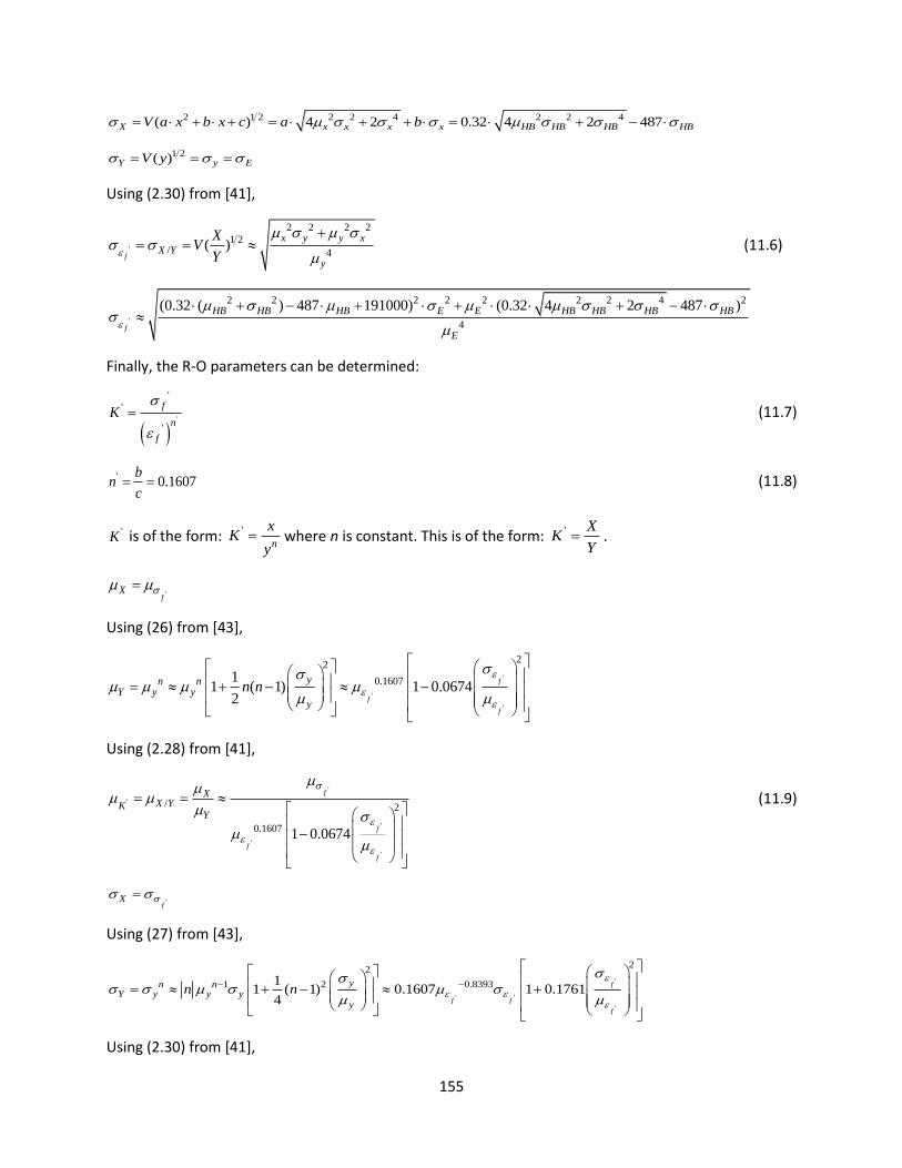
155

2 1 2 2 2 4 2 2 4( ) 4 2 0.32 4 2 487X x x x x HB HB HB HBV a x b x c a b

1 2( )Y y EV y

Using (2.30) from [41],

'

2 2 2 2

1 2/ 4

( )f

x y y x

X Y

y

XV

Y

(11.6)

'

2 2 2 2 2 2 2 4 2

4

(0.32 ( ) 487 191000) (0.32 4 2 487 )

f

HB HB HB E E HB HB HB HB

E

Finally, the R-O parameters can be determined:

'

'

'

'n

f

f

K

(11.7)

' 0.1607b

nc

(11.8)

'K is of the form: '

n

xK

y where n is constant. This is of the form: ' X

KY

.

'fX

Using (26) from [43],

'

'

'

22

0.160711 ( 1) 1 0.0674

2

f

f

f

yn nY y y

y

n n

Using (2.28) from [41],

'

'

'

'

'

/ 2

0.1607 1 0.0674

f

f

f

f

XX YK

Y

(11.9)

'fX

Using (27) from [43],

'

' '

'

22

1 2 0.839311 ( 1) 0.1607 1 0.1761

4

f

f f

f

yn nY y y y

y

n n

Using (2.30) from [41],

156

'

2 2 2 2

/ 4

x y y x

X YKy

' '

' ' ' ' '

' '

'

'

'

'

2 22 2

2 0.8393 2 0.1607

42

0.1607

0.1607 1 0.1761 1 0.0674

1 0.0674

f f

f f f f f

f f

f

f

f

K

(11.10)

Modified Universal Slopes Method

The M-C parameters for MUSM are given in Equation (3.12) and are repeated here:

0.832 0.09 0.155 0.53 0.56ε0.623( ) (2 ) 0.0196 ( ) (2 )

2

UTS UTSf f fN N

E E

Therefore, as can be seen b and c are constants while 'f and '

f are functions of random variables. In

(1.4), the elastic portion of the fatigue life is given as '

f

E

and so E needs to be factored out.

0.168' 0.8320.623f UTS E (11.11)

' 0.155 0.530.0196 ( )UTSf f

E

(11.12)


f .


f a X Y where 11n

X x , 22n

Y x , a, n1, n2 are constants.

Using Equations (26) from [43], and then Equation (2.8) and (2.25) from [41],

22

0.832 0.8321 0.0699 1 0.0699 UTS

UTS

UTS

xX x

x

2 2

0.168 0.1681 0.0699 1 0.0699y E

Y y EEy

'

2 2

0.832 0.1680.623 1 0.0699 1 0.0699UTS

UTSf

UTS

EX Y E

E

a

(11.13)

Using Equations (27) from [43], and then Equation (2.10) and (2.27) from [41],

157

22

0.168 0.168

1 10.832 1 0.00706 0.832 1 0.00706 UTS

UTS

UTSUTS

xX x

xx

(11.14)

2 2

0.832 0.832

1 10.168 1 0.1731 0.168 1 0.1731

y EY y E

y Ey E

(11.15)

'2 2 2 2 2 20.623

fX Y Y X X Y

(11.16)


f

a X Y

Z

where 1

1n

X x , 22n

Y x , 33n

Z x , a, n1, n2 , n3 are constants.

For statistics of functions of more than two variables, the algebra of expectations needs to be derived.

The mean value is derived from the following equation, (2.58) in [41].

2

1 2 21

1, ,..., ( )

2

n

n i

ii

yE y f E x E x E x V x

x

(11.17)

The standard deviation value is derived from the following equation, (2.62) in [41]. Higher order terms

are neglected in this derivation, so there is the possibility of error.

1 22

2

1i

n

y xii

y

x

(11.18)

Using (11.17),

'

0.155 0.53 0.155 0.530.532 2

0.53 1.845 0.53 2.53

0.155

2

1.47 0.53

0.0196 0.00128 0.00795

0.00244

f f

f UTSf

UTS f UTS UTS

f

UTS

E EE

E

E

(11.19)

Using (11.18),

'

1 22 2 2

0.155 0.53 0.1550.532 2 2

0.845 0.53 1.53 0.47 0.530.00304 0.01039 0.01039

f f

f UTSf

f UTS UTS UTS

EEE

E

(11.20)

It should be noted that f is often estimated from Equation (3.7), where 1

ε ln( )1

fRA

. If this is the

case, then the statistics of random variables cannot be used to determine the mean and standard

deviation of f from RA as a result of the natural logarithm. This may mean that an estimate for the

mean and standard deviation of 'f cannot be made.

158

Universal Slopes Method

The M-C parameters for USM are given in Equation (3.11) and are repeated here:

0.12 0.6 0.61.9018 (2 ) 0.7579 (2 )2

UTSf f fN N

E

Therefore, as can be seen, b and c are constants while 'f and '

f are functions of random variables.

' 1.9018f UTS (11.21)

' 0.60.7579f f (11.22)


f .


f a x where a is a constant.

Using Equations (2.8) from [41],

' 1.9018UTSf

xa (11.23)

Using (2.10) from [41],

' 1.9018UTSf

xa

(11.24)


f a X where 11n

X x , a, n1 are constants.

Using Equations (26) from [43], and then Equation (2.8) from [41],

22

0.6 0.61 0.12 1 0.12f

f

f

xX x

x

'

2

0.60.7579 1 0.12f

ff

f

Xa

(11.25)

Using Equations (27) from [43], and then Equation (2.10) from [41],

22

0.4 0.4

1 10.6 1 0.04 0.6 1 0.04

f

f

ff

xX x

xx

(11.26)

'

2

0.4

10.4547 1 0.04

f

ff

ff

(11.27)

It should be noted that f is often estimated from Equation (3.7), where 1

ε ln( )1

fRA

. If this is the

case, then the statistics of random variables cannot be used to determine the mean and standard

159

deviation of f from RA as a result of the natural logarithm. This may mean that an estimate for the

mean and standard deviation of 'f cannot be made.

Uniform Material Law

The M-C parameters for UML are given in Equation (3.19) for steels and Equation (3.20) for aluminum

and titanium alloys and are repeated here respectively:

0.087 0.581.50 (2 ) 0.59 (2 )2

UTSf fN N

E

Where UTSσ

1.0 for 0.003E

UTS UTSσ σ

(1.375 125.0 ) for 0.003E E

For aluminum and titanium alloys:

0.095 0.581.67 (2 ) 0.35(2 )2

UTSf fN N

E

Therefore, as can be seen, b and c are constants while 'f is a function of a random variable and '

f’ is

constant or a function of random variable.

First looking at the equation for steels:

' 1.5f UTS (11.28)

' 0.59f or ' 1.375 125.0 UTSf

E

(11.29)

Depending on the value of UTSσ

E as noted above.


f . The

forms and equations used are the same as in the analysis for USM, since it is just the multiplication of a

constant.

' 1.5UTSf

xa (11.30)

' 1.5UTSf

xa

(11.31)


f a for the first case and 'f

xa b

y here a, b are constants.

Using (2.8), (2.11) and (2.28) from [41],

' 0.59f

or ' / 125.0 1.375UTS

fX Y

E

a b

(11.32)

Using (2.10), (2.12) and (2.30) from [41],

160

' 0f

or '

22 2 2

4125.0 UTS UTS

f

E E

E

(11.33)

For titanium and aluminum alloys:

' 1.67f UTS (11.34)

' 0.35f (11.35)


f . The

forms and equations used are the same as above

' 1.67UTSf

xa (11.36)

' 1.67UTSf

xa

(11.37)

' 0.35f

(11.38)

' 0f

(11.39)

Median’s Method

The M-C parameters for MedM are given in Table 1.

As can be seen, 'f , b and c are constants while '

f is a function of a random variable.

'f UTSa (11.40)

where a is a different constant depending on the material class.

Using the same analysis for a constant and random variable as before:

'UTSf

xa a (11.41)

'UTSf

xa a

(11.42)

'f

a

(11.43)

' 0f

(11.44)

Remaining Methods

Closed form algebra of expectations cannot be used to determine the mean and variance for the

remaining estimation methods: FPM, MFPM, MM and MMM. This is a result of the structure of the

mathematical model that is used to predict the strain-life curve, through the M-C parameters. Certain

mathematical functions, such as random variables to the power of other random variables, logarithms of

161

random variables and the fatigue strength and fatigue ductility exponents being functions of random

variables, do not allow for closed form solutions. This is because the family of functions employed in the

previous sections cannot be used for these mathematical functions. Instead, Monte-Carlo simulations

would need to be used to generate estimates for the statistics of these functions [41]. Therefore Monte-

Carlo simulation is used for all methods for predicting the variability for consistency as presented in

Section 8.2 Fatigue Properties Variability from Monotonic Properties Variability and Section 9 Fatigue

Properties Estimation Software.

robust model for fatigue life estimation from monotonic

Documents