robust classification of animal tracking data - mit computer

Computers and Electronics in Agriculture 56 (2007) 46–59

Robust classification of animal tracking data

Mac Schwager a,∗, Dean M. Anderson b, Zack Butler c, Daniela Rus a

a Distributed Robotics Laboratory, Massachusetts Institute of Technology, Cambridge, MA 02139, United Statesb USDA-ARS, Jornada Experimental Range, Las Cruces, NM 88003, United States

c Computer Science Department, Rochester Institute of Technology, Rochester, NY 14623, United States

Received 2 June 2006; received in revised form 3 November 2006; accepted 5 January 2007

Abstract

This paper describes an application of the K-means classification algorithm to categorize animal tracking data into various classesof behavior. It was found that, even without explicit consideration of biological factors, the clustering algorithm repeatably resolvedtracking data from cows into two groups corresponding to active and inactive periods. Furthermore, it is shown that this classificationis robust to a large range of data sampling intervals. An adaptive data sampling algorithm is suggested for improving the efficiencyof both energy and memory usage in animal tracking equipment.© 2007 Elsevier B.V. All rights reserved.

Keywords: Cluster analysis; GPS; Animal tracking; Adaptive sampling; Sensor networks

1. Introduction

The use of mobile sensors promises a data-rich future for the animal behavioral sciences. However, with large datasets also comes the burden of data analysis and interpretation. In the future, the human analyst will rely on computationaltechniques to meaningfully interpret large data sets and discover meaningful statistical trends. In this work we proposeone simple computational tool to help animal researchers interpret large data sets.

Specifically, we introduce the use of the K-means classification algorithm (Arabie et al., 1996) to classify animaltracking data without a priori information into two categories. These categories are found to correspond to periodsof animal activity and inactivity. We use position and head angle data from several cows to demonstrate how thisalgorithm could be employed in a behavioral study involving free-ranging animals. Furthermore, we investigate aparticularly useful property of this classification algorithm—its robustness with respect to data sample rates. Thisrobustness suggests that the classifier can be used to drive an adaptive sample rate data collection system, which willhave the potential to save energy without sacrificing the information content of the collected data. Robustness of thealgorithm to different sample rates is also demonstrated using cow tracking and head angle data.

We have not attempted to carry out a conclusive study of free-ranging cow activity and inactivity in this work, but,rather, suggest a method in general terms and use cow data to demonstrate how the algorithm can be useful in a typicalanimal behavioral study. It should also be noted that the applicability of the method is not tied to the specific example orequipment described herein. The method can equally be employed to classify tracking data from any species, including

∗ Corresponding author. Tel.: +1 617 253 6532; fax: +1 617 253 6849.E-mail addresses: [email protected] (M. Schwager), [email protected] (D.M. Anderson), [email protected] (Z. Butler),

[email protected] (D. Rus).

0168-1699/$ – see front matter © 2007 Elsevier B.V. All rights reserved.doi:10.1016/j.compag.2007.01.002

mailto:[email protected]




dx.doi.org/10.1016/j.compag.2007.01.002

M. Schwager et al. / Computers and Electronics in Agriculture 56 (2007) 46–59 47

humans, regardless of the tracking instrument used. Indeed, our broader research agenda is to develop computationalapproaches for studying groups of various kinds of dynamical agents with social interactions. We expect that suchdynamical groups can be studied and modelled using physical data, and ultimately controlled.

1.1. Relationship to current state of knowledge

Several recent animal behavior studies have made use of automated data collection systems to allow for compu-tationally intensive post-processing analysis (Butler et al., 2006; Bishop-Hurley et al., 2005; Anderson, 2001). Aninterdisciplinary group at Princeton University has developed a network for monitoring the movements and socialgroupings of Zebras in Kenya (Juang et al., 2002). Researchers at the University of California, San Diego have usedpattern recognition algorithms to identify and classify worm behavior (Geng et al., 2003). Statistical clustering tech-niques have also been adapted to classify dolphin whistle calls (McCowan, 1995), and to identify animal aggregations(Strauss, 2001).

More directly related to our work, some recent studies have been conducted to infer activity states of free-ranginganimals using global positioning system (GPS) tracking data. Ganskopp (2001) found that the Euclidean distancebetween successive GPS fixes was not sufficient to infer cattle activity states using a regression analysis. Schlecht etal. (2004) compared classification results from human observers with those found from discriminant analysis of GPSdata and found that the two were in agreement for 71% of the data. This work required an initial calibration step using aportion of the collected data to manually select discriminants that were then used to classify the remainder of the data.Finally, Ungar et al. (2005) used GPS position and acceleration data from cattle to infer states of activity. They foundthat discriminant analysis classification agreed with human observation for at least 74% of the data while regressiontree classification agreed with human observation for at least 84% of the data. The K-means algorithm discussed inthis paper differs from the above statistical methods in that it performs classification in a highly autonomous fashion.In particular it requires only minimal data preparation and does not require an off-line calibration step, nor does itrequire the human analyst to pre-select suitable discriminants on which to base a regression model. In the machinelearning community, K-means is considered a simple example of an unsupervised learning algorithm, whereas theabove methods would be considered supervised algorithms (Duda et al., 2001).

This research points toward a potential application of the K-means algorithm to help ease power and memoryrequirements for data collection equipment. Current research has identified the difficulty of balancing data resolutionwith technical limitations, particularly on-animal power and memory requirements (Anderson, 2006). In order to mit-igate power and memory constraints, most commercial on-animal GPS devices are restricted to a maximum positionrecording rate of once every 5 min (this trend is changing, however (Clark et al., 2006)). This rather infrequent dataacquisition rate may cause significant amounts of information about landscape utilization to be missed, especiallyduring foraging (Schlecht et al., 2004) and possibly even during non-foraging travel (Estevez and Christian, 2005).This is a problem of critical importance since most current animal behavior rangeland research is focused on under-standing animal distribution in order to accurately characterize landscape utilization and ultimately manage utilization(Anderson, 2006; Bailey, 2005; DelCurto et al., 2005; Bailey, 2004; Bailey et al., 2001; Hulbert and French, 2001;Turner et al., 2000; Coppolillo, 2000; Bailey et al., 1996; Coughenour, 1991; Pinchak et al., 1991; Roath and Krueger,1982).

Thus, choosing an appropriate data sampling rate appears to be a principle factor in understanding free-ranginganimal behavior. This highlights the advantage of creating a data collection system that has an adaptive sample rate. Withsuch a system, data may be collected infrequently during periods for which high sample rates do not help to determineland utilization, while data can be sampled more frequently during periods that are more critical to understanding landutilization. The results of this paper suggest that the K-means algorithm would be well suited to trigger a change indata sample rates in such a data collection system because its classification qualities are insensitive to sample rates.

2. Methods

Our technical approach was as follows: (1) data from several free-ranging cows were collected; (2) data were thenanalyzed using the K-means algorithm to classify animal behavior into active and inactive states; (3) biological factorsassociated with activity and inactivity were compared with the autonomous classification to determine if the categoriescorresponded with actual periods of activity and inactivity; (4) the effects of decreasing sample rates on the resulting

48 M. Schwager et al. / Computers and Electronics in Agriculture 56 (2007) 46–59

sampled path was investigated for active and inactive states; (5) the effects of decreasing sample rates on the K-meansclassification algorithm was investigated for active and inactive states.

2.1. Tracking data

2.1.1. Data collection locationFree-ranging cow data were collected in a 466 ha (l103 ac) area (Paddock 10B), on the U.S. Department of Agricul-

ture, Agricultural Research Service’s (USDA-ARS), Jornada Experimental Range (JER). This site has an undulatingtopography of predominantly sandy soil with a mean elevation of 1260 m (4134 ft) above sea level(106◦43.263′′W,32◦34.297′′N) located approximately 37 km (23 mi) north of Las Cruces, NM. The climate of the region is typical ofarid rangeland having a long-term mean precipitation approaching 230 mm (9.1 in.) with 52% occurring between Julyand September. Mean maximum ambient air temperatures vary from a high of 36 ◦C (96.8 ◦F) in June to below 13 ◦C(55.4 ◦F) in January.

The major grass species found in Paddock 10B are Bouteloua eriopoda (Torr.) Torr., Sporobolus flexuosus (Thurb.)Ryudb. and Aristida purpurea Steud. Shrubs include Prosopis juliflora var glandulosa (Torr.) Cock, Yucca elataEngelm. and Gutierrezia sarothrae (Pursh) Britt. + Rusky. The few low-lying areas with heavier soils are dominatedby Scleropogon brevifolious Phil, and Sporobolus airoides (Torr.) Torr.

2.1.2. The animalsThree free-ranging mature beef cattle of Hereford and Hereford × Brangus genetics, labeled Cow 1, Cow 2, and

Cow 3, were monitored during two periods in 2004. Data were collected in 2004 beginning April 26 at 17:12 h throughApril 28 at 08:55 h (Trial 1), and again from May 17 at 12:50 h through May 19 at 07:44 h (Trial 2). During theseintervals, uncorrected global positioning system (GPS) data were recorded with Directional Virtual Fence (DVFTM)devices capable of providing sensory cues to alter the animal’s direction of movement on the landscape (Anderson,2006; Anderson et al., 2004; Anderson and Hale, 2001; Anderson, 2001). However, during these two trials, the animalsreceived no cues from the DVFTM devices.

The data included date, time, Universal Transverse Mercator (UTM) location together with the horizontal and verticalangle of the animal’s head. Head angles were measured in degrees from a reference position corresponding to the headbeing level with the animal’s backbone while looking straight ahead. A downward tilted head angle was denoted asnegative and an upward tilted head angle positive. Similarly, a left tilting head angle was denoted as negative while aright tilting head angle was positive. Head angles can be indicative of certain kinds of behavior. For instance, whileforaging, the cow’s head is likely to be angled downward toward the ground and while resting it is likely to be lookingstraight ahead or elsewhere (Anderson, 2006). An electronic magnetometer within the DVFTM device provided thesehead angle measurements. During Trial 2, the instrument worn by Cow 1 broke leaving a total of only five completedata sets from Trial 1 and Trial 2 upon which these analyses were made.

For each trial, data consisted of approximately 3000 entries for each cow collected at intervals alternating between43 and 53 s, with some additional sampling irregularities. Data points that located the animal outside of the paddockfences were removed manually as obvious outliers, however, no other data processing was carried out beyond what isstated explicitly below.

2.2. The K-means classifier

The K-means algorithm was used to classify each animal’s data into two categories without using a priori informa-tion. The resulting categories were examined and were determined to correspond to clearly defined periods of activityand inactivity. The algorithm was applied with the intention of testing the simplest possible approach, thus specialconsiderations were not made to filter out inherent GPS measurement noise.

Specifically, we used the K-means classification algorithm to group the data into two categories. The classificationwas performed over three dimensions of the collected data: speed, horizontal head angle, and vertical head angle. Thespeed was calculated from a numerical differentiation according to the formula:

sk = ‖xk+1 − xk‖tk+1 − tk

(1)


where s is the speed in m/s, x the GPS position vector, t the time stamp from the on board clock, k indicates the data indexnumber and ‖·‖ denotes the Euclidean distance. The horizontal and vertical head angles, θh and θv, respectively, werecollected directly from the DVFTM. We note that time of day was not considered in this analysis, nor was temporalauto-correlation of the data, that is, all data points for a single cow are simply put into a set for the calculationsirrespective of their temporal separation from one another. Our intention was to determine what clusters could be foundin the data using the most naive possible approach.

Before being used for classification, the data were normalized by subtracting the mean from each dimension, s, θh,and θv, and dividing each dimension by its standard deviation, In particular:

zk = yk − μ√(1/k)

∑k(yk − μ)2

, (2)

where μ = (1/k)∑

kyk is the mean, y represents the dimension, and z represents the dimension after normalization.This standard procedure was used to remove effects from constant offsets and scaling. Each data entry was arrangedas a vector vi = [si θhi

θvi ], and the resulting normalized data vectors were used for classification.

Algorithm 1: K-means classification

Require: Initial mean positions, μj, j = 1, . . ., KRequire: A norm, ‖·‖, by which to measure the distance between any two data vectorsRequire: A desired final tolerance, e, for the meansrepeat

Group each data vector with its closest mean (the one for which∥∥vi − μj

∥∥ is smallest)Compute the centroid of each group according to (1/nj)

∑Nj

vi, where Nj is the set of indices and nj is the size of the group

Take these new centroids as the new mean positions μj

until∥∥μnew

j − μoldj

∥∥ < e for all j = 1, . . ., K

The K-means algorithm was carried out using the Euclidean norm with each dimension equally weighted. Thealgorithm is listed here as Algorithm 1. This algorithm is guaranteed to stop for arbitrarily small e values. Unfortunately,the final mean positions and resulting groupings are known to be sensitive to the initial mean positions chosen by theuser. A more elaborate discussion of K-means and other classification methods can be found in Aldenderfer andBlashfield (1984), Arabie et al. (1996), and the original presentation of the algorithm is given in McQueen (1967). Thealgorithm was carried out as described above independently on the data for each individual cow.

3. Results

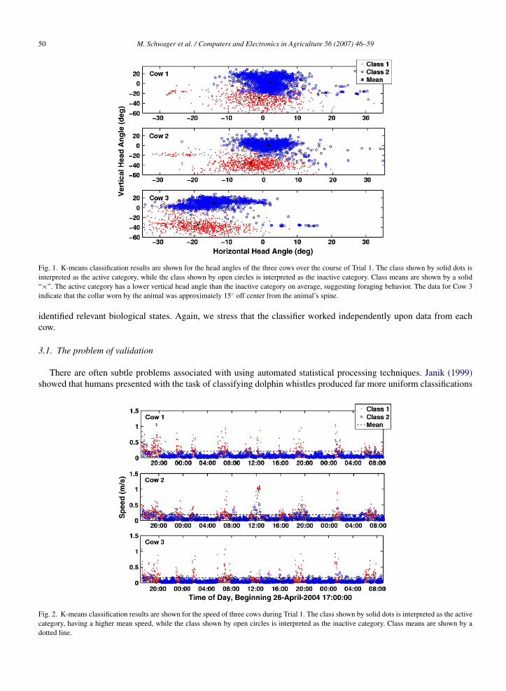
K-means repeatably produced two clusters from the data sets, clearly delineated into a category with low speedand high head angle, which we call inactive, and one with high speed and low head angle, which we call active. Theclassifier identifies the horizontal head angle (right versus left) as being inconsequential to the classes. Classificationresults for the three cows during Trial 1 are shown in Figs. 1 and 2, and results for the two cows in Trial 2 are shownin Figs. 3 and 4. Note that the classification is cohesive among periods of time. That is, adjacent data points werevery likely to be in the same category despite the inherent random GPS position errors in the data. Thus the algorithmappears to be sufficiently robust with respect to random position errors and is not hindered by the fact that temporalrelationships between successive data points were not used in the input to the classifier. Also, note that the periods ofactivity and inactivity are similar for all animals within the same trial. The classification was carried out independentlyfor each animal, thus the classifier has no knowledge of the context of the experiment nor of the location of one cowrelative to another. Therefore, the correlations that exist among animals serve a means of validating our results. Thisinterpretation suggests that the classifier has identified biologically relevant behavioral categories, since activity levelswithin a group of gregarious animals mutually influence one another (Smith, 1998; Immelmann and Beer, 1989).

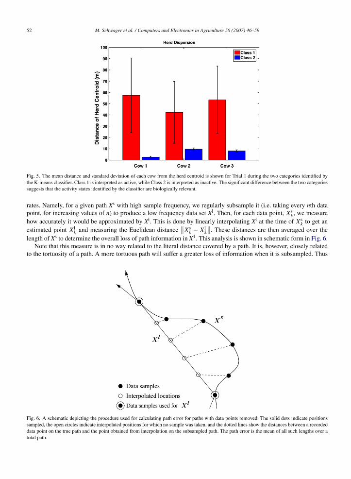
To further investigate whether or not the active and inactive states identified by the classifier were biologicallyrelevant, we compared statistics reflecting aggregation behavior within the two categories. In particular, the meandistance from each cow to the herd centroid and its standard deviation show that the animals were significantly andreliably closer together during periods of common inactivity than during activity. These data are shown in Fig. 5. Theclear difference in the placement and activity of the herd during these periods gives evidence that the classifier has


Fig. 1. K-means classification results are shown for the head angles of the three cows over the course of Trial 1. The class shown by solid dots isinterpreted as the active category, while the class shown by open circles is interpreted as the inactive category. Class means are shown by a solid“×”. The active category has a lower vertical head angle than the inactive category on average, suggesting foraging behavior. The data for Cow 3indicate that the collar worn by the animal was approximately 15◦ off center from the animal’s spine.

identified relevant biological states. Again, we stress that the classifier worked independently upon data from eachcow.

3.1. The problem of validation

There are often subtle problems associated with using automated statistical processing techniques. Janik (1999)showed that humans presented with the task of classifying dolphin whistles produced far more uniform classifications

Fig. 2. K-means classification results are shown for the speed of three cows during Trial 1. The class shown by solid dots is interpreted as the activecategory, having a higher mean speed, while the class shown by open circles is interpreted as the inactive category. Class means are shown by adotted line.


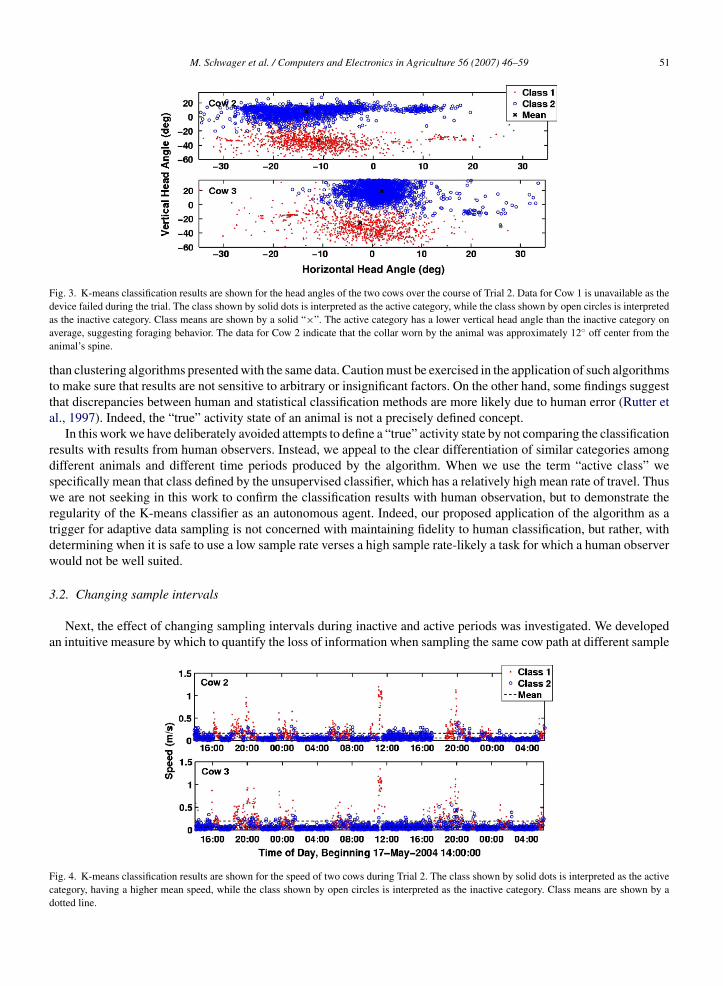
Fig. 3. K-means classification results are shown for the head angles of the two cows over the course of Trial 2. Data for Cow 1 is unavailable as thedevice failed during the trial. The class shown by solid dots is interpreted as the active category, while the class shown by open circles is interpretedas the inactive category. Class means are shown by a solid “×”. The active category has a lower vertical head angle than the inactive category onaverage, suggesting foraging behavior. The data for Cow 2 indicate that the collar worn by the animal was approximately 12◦ off center from theanimal’s spine.

than clustering algorithms presented with the same data. Caution must be exercised in the application of such algorithmsto make sure that results are not sensitive to arbitrary or insignificant factors. On the other hand, some findings suggestthat discrepancies between human and statistical classification methods are more likely due to human error (Rutter etal., 1997). Indeed, the “true” activity state of an animal is not a precisely defined concept.

In this work we have deliberately avoided attempts to define a “true” activity state by not comparing the classificationresults with results from human observers. Instead, we appeal to the clear differentiation of similar categories amongdifferent animals and different time periods produced by the algorithm. When we use the term “active class” wespecifically mean that class defined by the unsupervised classifier, which has a relatively high mean rate of travel. Thuswe are not seeking in this work to confirm the classification results with human observation, but to demonstrate theregularity of the K-means classifier as an autonomous agent. Indeed, our proposed application of the algorithm as atrigger for adaptive data sampling is not concerned with maintaining fidelity to human classification, but rather, withdetermining when it is safe to use a low sample rate verses a high sample rate-likely a task for which a human observerwould not be well suited.

3.2. Changing sample intervals

Next, the effect of changing sampling intervals during inactive and active periods was investigated. We developedan intuitive measure by which to quantify the loss of information when sampling the same cow path at different sample

Fig. 4. K-means classification results are shown for the speed of two cows during Trial 2. The class shown by solid dots is interpreted as the activecategory, having a higher mean speed, while the class shown by open circles is interpreted as the inactive category. Class means are shown by adotted line.


Fig. 5. The mean distance and standard deviation of each cow from the herd centroid is shown for Trial 1 during the two categories identified bythe K-means classifier. Class 1 is interpreted as active, while Class 2 is interpreted as inactive. The significant difference between the two categoriessuggests that the activity states identified by the classifier are biologically relevant.

rates. Namely, for a given path Xs with high sample frequency, we regularly subsample it (i.e. taking every nth datapoint, for increasing values of n) to produce a low frequency data set Xl. Then, for each data point, Xs

k, we measurehow accurately it would be approximated by Xl. This is done by linearly interpolating Xl at the time of Xs

k to get anestimated point Xl

k and measuring the Euclidean distance∥∥Xs

k − Xlk

∥∥. These distances are then averaged over thelength of Xs to determine the overall loss of path information in X1. This analysis is shown in schematic form in Fig. 6.

Note that this measure is in no way related to the literal distance covered by a path. It is, however, closely relatedto the tortuosity of a path. A more tortuous path will suffer a greater loss of information when it is subsampled. Thus

Fig. 6. A schematic depicting the procedure used for calculating path error for paths with data points removed. The solid dots indicate positionssampled, the open circles indicate interpolated positions for which no sample was taken, and the dotted lines show the distances between a recordeddata point on the true path and the point obtained from interpolation on the subsampled path. The path error is the mean of all such lengths over atotal path.


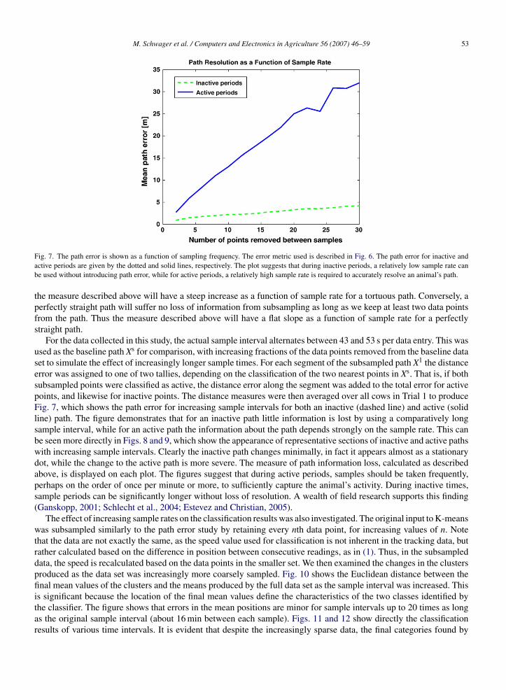
Fig. 7. The path error is shown as a function of sampling frequency. The error metric used is described in Fig. 6. The path error for inactive andactive periods are given by the dotted and solid lines, respectively. The plot suggests that during inactive periods, a relatively low sample rate canbe used without introducing path error, while for active periods, a relatively high sample rate is required to accurately resolve an animal’s path.

the measure described above will have a steep increase as a function of sample rate for a tortuous path. Conversely, aperfectly straight path will suffer no loss of information from subsampling as long as we keep at least two data pointsfrom the path. Thus the measure described above will have a flat slope as a function of sample rate for a perfectlystraight path.

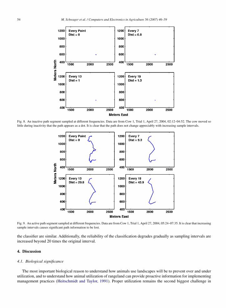
For the data collected in this study, the actual sample interval alternates between 43 and 53 s per data entry. This wasused as the baseline path Xs for comparison, with increasing fractions of the data points removed from the baseline dataset to simulate the effect of increasingly longer sample times. For each segment of the subsampled path X1 the distanceerror was assigned to one of two tallies, depending on the classification of the two nearest points in Xs. That is, if bothsubsampled points were classified as active, the distance error along the segment was added to the total error for activepoints, and likewise for inactive points. The distance measures were then averaged over all cows in Trial 1 to produceFig. 7, which shows the path error for increasing sample intervals for both an inactive (dashed line) and active (solidline) path. The figure demonstrates that for an inactive path little information is lost by using a comparatively longsample interval, while for an active path the information about the path depends strongly on the sample rate. This canbe seen more directly in Figs. 8 and 9, which show the appearance of representative sections of inactive and active pathswith increasing sample intervals. Clearly the inactive path changes minimally, in fact it appears almost as a stationarydot, while the change to the active path is more severe. The measure of path information loss, calculated as describedabove, is displayed on each plot. The figures suggest that during active periods, samples should be taken frequently,perhaps on the order of once per minute or more, to sufficiently capture the animal’s activity. During inactive times,sample periods can be significantly longer without loss of resolution. A wealth of field research supports this finding(Ganskopp, 2001; Schlecht et al., 2004; Estevez and Christian, 2005).

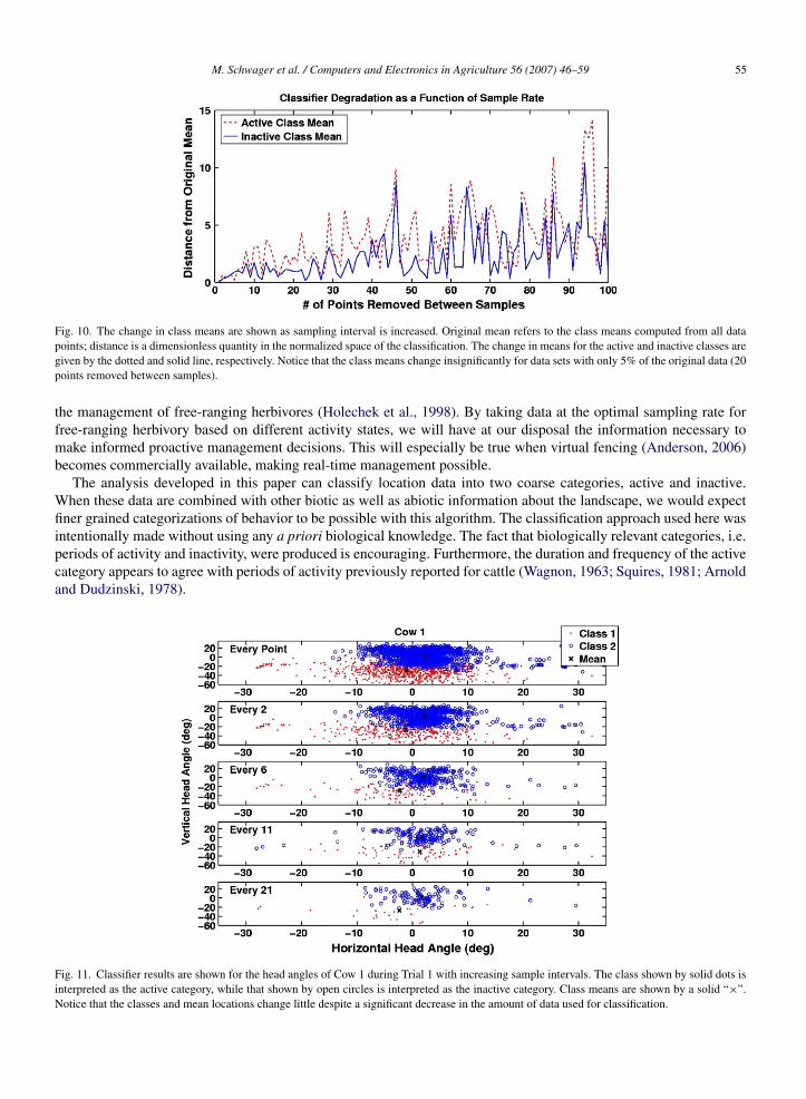
The effect of increasing sample rates on the classification results was also investigated. The original input to K-meanswas subsampled similarly to the path error study by retaining every nth data point, for increasing values of n. Notethat the data are not exactly the same, as the speed value used for classification is not inherent in the tracking data, butrather calculated based on the difference in position between consecutive readings, as in (1). Thus, in the subsampleddata, the speed is recalculated based on the data points in the smaller set. We then examined the changes in the clustersproduced as the data set was increasingly more coarsely sampled. Fig. 10 shows the Euclidean distance between thefinal mean values of the clusters and the means produced by the full data set as the sample interval was increased. Thisis significant because the location of the final mean values define the characteristics of the two classes identified bythe classifier. The figure shows that errors in the mean positions are minor for sample intervals up to 20 times as longas the original sample interval (about 16 min between each sample). Figs. 11 and 12 show directly the classificationresults of various time intervals. It is evident that despite the increasingly sparse data, the final categories found by


Fig. 8. An inactive path segment sampled at different frequencies. Data are from Cow 1, Trial 1, April 27, 2004, 02:12–04:52. The cow moved solittle during inactivity that the path appears as a dot. It is clear that the path does not change appreciably with increasing sample intervals.

Fig. 9. An active path segment sampled at different frequencies. Data are from Cow 1, Trial 1, April 27, 2004, 05:24–07:35. It is clear that increasingsample intervals causes significant path information to be lost.

the classifier are similar. Additionally, the reliability of the classification degrades gradually as sampling intervals areincreased beyond 20 times the original interval.

4. Discussion

4.1. Biological significance

The most important biological reason to understand how animals use landscapes will be to prevent over and underutilization, and to understand how animal utilization of rangeland can provide proactive information for implementingmanagement practices (Heitschmidt and Taylor, 1991). Proper utilization remains the second biggest challenge in


Fig. 10. The change in class means are shown as sampling interval is increased. Original mean refers to the class means computed from all datapoints; distance is a dimensionless quantity in the normalized space of the classification. The change in means for the active and inactive classes aregiven by the dotted and solid line, respectively. Notice that the class means change insignificantly for data sets with only 5% of the original data (20points removed between samples).

the management of free-ranging herbivores (Holechek et al., 1998). By taking data at the optimal sampling rate forfree-ranging herbivory based on different activity states, we will have at our disposal the information necessary tomake informed proactive management decisions. This will especially be true when virtual fencing (Anderson, 2006)becomes commercially available, making real-time management possible.

The analysis developed in this paper can classify location data into two coarse categories, active and inactive.When these data are combined with other biotic as well as abiotic information about the landscape, we would expectfiner grained categorizations of behavior to be possible with this algorithm. The classification approach used here wasintentionally made without using any a priori biological knowledge. The fact that biologically relevant categories, i.e.periods of activity and inactivity, were produced is encouraging. Furthermore, the duration and frequency of the activecategory appears to agree with periods of activity previously reported for cattle (Wagnon, 1963; Squires, 1981; Arnoldand Dudzinski, 1978).

Fig. 11. Classifier results are shown for the head angles of Cow 1 during Trial 1 with increasing sample intervals. The class shown by solid dots isinterpreted as the active category, while that shown by open circles is interpreted as the inactive category. Class means are shown by a solid “×”.Notice that the classes and mean locations change little despite a significant decrease in the amount of data used for classification.


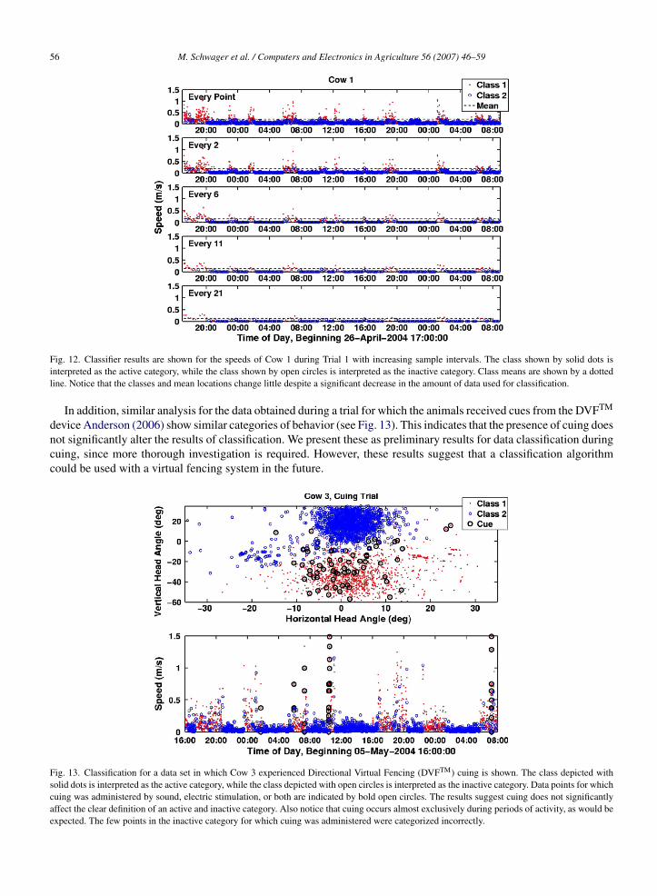
Fig. 12. Classifier results are shown for the speeds of Cow 1 during Trial 1 with increasing sample intervals. The class shown by solid dots isinterpreted as the active category, while the class shown by open circles is interpreted as the inactive category. Class means are shown by a dottedline. Notice that the classes and mean locations change little despite a significant decrease in the amount of data used for classification.

In addition, similar analysis for the data obtained during a trial for which the animals received cues from the DVFTM

device Anderson (2006) show similar categories of behavior (see Fig. 13). This indicates that the presence of cuing doesnot significantly alter the results of classification. We present these as preliminary results for data classification duringcuing, since more thorough investigation is required. However, these results suggest that a classification algorithmcould be used with a virtual fencing system in the future.

Fig. 13. Classification for a data set in which Cow 3 experienced Directional Virtual Fencing (DVFTM) cuing is shown. The class depicted withsolid dots is interpreted as the active category, while the class depicted with open circles is interpreted as the inactive category. Data points for whichcuing was administered by sound, electric stimulation, or both are indicated by bold open circles. The results suggest cuing does not significantlyaffect the clear definition of an active and inactive category. Also notice that cuing occurs almost exclusively during periods of activity, as would beexpected. The few points in the inactive category for which cuing was administered were categorized incorrectly.


We expect that incorporating additional biological knowledge into the algorithm will enable the computation offiner-grained classification and more complete real-time understanding of the animals’ behavior. For example, it is clearthat biotic and abiotic landscape parameters (density of forage, topography, wind speed and direction, etc.) affect cattle(Hafez and Bouissou, 1975; Squires, 1981). By adding these dimensions to our data set, we may be able to evaluate howactivity varies in a correlated way with landscape parameters. Besides individual behavior, we are also interested in therelative positions of the animals and the movement of the herd. Including this information in a classification algorithmcould lead to intraspecial, as well as interspecial, animal behavior models to characterize how animal behavior changesas a function of neighbor proximity and herd dispersion or aggregation.

4.2. Other data collection devices

Previous GPS-based animal behavioral research projects have used both modified and off-the-shelf GPS units. Forinstance, Schlecht et al. (2004) used customized backpacks with modified GPS units which recorded animal positionsevery 10 s, while Ungar et al. (2005) used commercially available LotekTM2000 and 2200LR collars that logged data at20 and 5 min intervals, respectively, combined with on-collar accelerometer measurements to aid in classification. Ourdata were collected from DVFTM devices (Anderson, 2006), which are not yet commercially available. This breadthof devices and sample intervals used for collecting data raises the question of whether or not the devices themselvesmay influence the results of studies.

Our analysis of path lengths above attempts to addresses this question. It is always advantageous to collect data asfrequently as possible. Statistically, more frequent data sampling can only improve the fidelity of an analysis. Thusdata collection rates ought to be limited only by device energy and memory restrictions ultimately imposed by costconstraints. It would seem that logging data at 10 s intervals is sufficient to capture the most erratic of cow paths withgreat detail (Schlecht et al., 2004), however energy and memory would be wasted on periods during which the animalis inactive. Conversely, logging data every 20 min (Ungar et al., 2005) will lose much fine-grained information abouta cow’s path, but will give devices a long lifetime in the field. The researcher ought to collect data at a resolutionappropriate for the objectives of the study. In any case, the K-means algorithm has been shown above to be insensitiveto sample rates, thus it can be used safely with any reasonable data collection device to classify activity levels.

4.3. Adaptive sampling

The robustness of the K-means algorithm to sample rates ranging from once per minute (or less) to once every16 min suggests that the K-means algorithm can be used to drive a variable sample interval data collection device—onewhich records samples at a high frequency during periods of activity and records at a lower frequency during periodsof inactivity. The results show that during inactive periods there is little benefit to a high sample rate, while duringactive periods a high sample rate is required to resolve important properties of an animal’s path.

From an engineering point of view, these results suggest guidelines for animal device design as well as experimentdesign. Both memory and power could be used more efficiently if the data collecting device were able to change itssample rate given the activity state of the animal. Fortunately, the K-means classifier has an on-line variant, which canbe used to classify data as it is obtained. The identified category of the incoming data can then be used to dictate thefuture sample rate at which data will be recorded. Such an adaptive sampling algorithm could provide significant gainsin over-all device lifetime.

5. Conclusion

The K-means classification algorithm was used to cluster GPS tracking data obtained from mature cows into twocategories representing activity and inactivity. We found that the categories computed by the algorithm were consistentamong animals within a trial for two different trials. These results do not address questions about cattle behavior atlarge, but, rather, demonstrate that the K-means algorithm can be useful in determining animal activity states in anautonomous way. This research also suggests that a sufficiently high data sampling rate is important for characterizingland utilization by cattle during periods of activity, while sample rate is not important during periods of inactivity. Lastlywe have demonstrated that K-means classification is robust with respect to sample intervals of various length. Theseresults suggest that an on-line K-means algorithm can be used to identify between periods of activity and inactivity


and subsequently adjust the data sampling rate accordingly. Such an adaptive sampling scheme will provide improvedresolution while conserving memory and energy in future data collection devices.

Acknowledgments

This work was supported in part by NSF grant IIS-0513628 and the SWARMS MURI grant. The authors alsothank the staff of the USDA-ARS Jornada Experimental Range, especially Mr. Roy Libeau, biological animal sciencestechnician Jornada Experimental Range and Ms. Barbara Nolen, GIS administrator Jornada Experimental Range fortheir dedicated commitment to the DVFTM research program that provided these data.

References

Aldenderfer, M.S., Blashfield, R.K., 1984. Cluster Analysis. Sage Publications, Newbury Park, CA.Anderson, D.M., 2001. Virtual fencing—a prescription range animal management tool for the 21st century. In: Sibblald, A., Gordon, I. (Eds.),

Proceedings of the Conference Tracking Animals with GPS. Macaulay Land Use Research Institute, Aberdeen, Scotland, pp. 85–94.Anderson, D.M., 2006. Virtual fencing—a concept into reality. In: Spatial Grazing Behaviour Workshop Proceedings, Rockhampton, Qld., CSIRO.Anderson, D.M., Hale, C.S., 2001. Inventors; The United States of America as represented by the Secretary of Agriculture. Animal control system

using global positioning and instrumental animal conditioning. U.S. Patent 6,232,880.Anderson, D.M., Nolen, B., Fredrickson, E., Havstad, K., Hale, C.S., 2004. Representing spatially explicit directional virtual fencing DVFTM data.

In: The 24th Annual ESRI International User Conference Proceedings.Arabie, P., Hubert, L.J., Soete, G.D., 1996. Clustering and Classification. World Scientific, Singapore.Arnold, G.W., Dudzinski, M.L., 1978. Ethology of Free-ranging Domestic Animals. Elsevier Scientific, New York.Bailey, D.W., 2004. Management strategies for optimal grazing distribution and use of arid rangelands. J. Anim. Sci. 82, E147–E153.Bailey, D.W., 2005. Identification and creation of optimum habitat conditions for livestock. Range. Ecol. Manage. 58, 109–118.Bailey, D.W., Gross, J.E., Laca, E.A., Rittenhouse, L.R., Coughenour, M.B., Swift, D.M., Sims, P.L., 1996. Mechanisms that result in large herbivore

grazing distribution patterns. J. Range Manage. 49, 386–400.Bailey, D.W., Kress, D.D., Anderson, D.C., Boss, D.L., Miller, E.T., 2001. Relationship between terrain use and performance of beef cows grazing

foothill rangeland. J. Anim. Sci. 79, 1883–1891.Bishop-Hurley, G.J., Swain, D.L., Anderson, D.M., Corke, P., Sikka, P., Crossman, C., 2005. Understanding interactions between autonomous

animal control and temperament when cattle are subjected to virtual fencing applications. In: Horizons in Livestock Sciences RedesigningAnimal Agriculture. Gold Coast, Queensland, p. 23.

Butler, Z., Corke, P., Peterson, R., Rus, D., 2006. From robots to animals: virtual fences for controlling cows. Int. J. Robot. Res. 25 (5/6).Clark, P.E., Johnson, D.E., Kniep, M.A., Jermann, P., Huttash, B., Wood, A., Johnson, M., McGillivan, C., Titus, K., 2006. An advanced, low-cost,

GPS-based animal tracking system. Range. Ecol. Manage. 59, 334–340.Coppolillo, P.B., 2000. The landscape ecology of pastoral herding: spatial analysis of land use and livestock production in east Africa. Hum. Ecol.

28, 527–560.Coughenour, M.B., 1991. Spatial components of plant-herbivore interactions in pastoral, ranching, and native ungulate ecosystems. J. Range Manage.

44, 530–542.DelCurto, T., Porath, M., Parsons, C.T., Morrison, J.A., 2005. Management strategies for sustainable beef cattle grazing on forested rangelands in

the pacific northwest. Range. Ecol. Manage. 58, 119–127.Duda, R., Hart, P., Stork, D., 2001. Pattern Classification. Wiley and Sons, New York.Estevez, I., Christian, M.C., 2005. Analysis of the movement and use of space of animals in confinement: the effect of sampling effort. Appl. Anim.

Behav. Sci. 97, 221–240.Ganskopp, D., 2001. Manipulating cattle distribution with salt and water in large arid-land pastures: a GPS/GIS assessment. Appl. Anim. Behav.

Sci. 73, 251–262.Geng, W., Cosman, P., Huang, C., Schafer, W., 2003. Automated worm tracking and classification. In: Proceedings of the 37th Asilomar Conference

on Signals, Systems and Computers, Pacific Grove, CA, pp. 2063–2068.Hafez, E.S.E., Bouissou, M.F., 1975. The behaviour of cattle. In: Hafez, E.S.E. (Ed.), The Behaviour of Domestic Animals. Williams and Wilkins,

Baltimore.Heitschmidt, R.K., Taylor Jr., C.A., 1991. Livestock production. In: Heitschmidt, R.K., Stuth, J.W. (Eds.), Grazing Management an Ecological

Perspective. Timber Press, Portland, Oregon, pp. 161–177.Holechek, J.L., Pieper, R.D., Herbel, C.H., 1998. Range Management Principles and Practices, 3rd ed. Prentice Hall, Englewood Cliffs, NJ.Hulbert, I.A.R., French, J., 2001. The accuracy of GPS for wildlife telemetry and habitat mapping. J. Appl. Ecol. 38, 869–878.Immelmann, K., Beer, C., 1989. A Dictionary of Ethology. Harvard University Press, Cambridge, MA.Janik, V.M., 1999. Pitfalls in the categorization of behaviour: a comparison of dolphin whistle classification methods. Anim. Behav. 57, 133–143.Juang, P., Oki, H., Wang, Y., Martonosi, M., Peh, L.-S., Rubenstein, D., 2002. Energy efficient computing for wildlife tracking: design and early

experiences with zebranet. In: Proceedings of the Conference on Architectural Support for Programming Languages and Operating Systems,San Jose, CA.

McCowan, B., 1995. A new quantitative technique for categorizing whistles using simulated signals and whistles from captive bottlenose dolphins(Delphinidae, Tursiops truncatus). Ethology 100, 177–193.


McQueen, J.B., 1967. Some methods for classification and analysis of multivariate observations. In: Proceedings of the 5th Berkeley Symposiumon Mathematical Statistics and Probability, vol. 1. University of California Press, Berkeley, CA, pp. 281–297.

Pinchak, W.E., Smith, M.A., Hart, R.H., Waggoner, J.W., 1991. Beef cattle distribution patterns on foothill range. J. Range Manage. 44, 267–275.Roath, L.R., Krueger, W.C., 1982. Cattle grazing and behavior on a forested range. J. Range Manage. 35, 332–338.Rutter, S.M., Champion, R.A., Penning, P.D., 1997. An automatic system to record foraging behaviour in free-ranging ruminants. Appl. Anim.

Behav. Sci. 54, 185–195.Schlecht, E., Hulsebusch, C., Mahler, F., Becker, K., 2004. The use of differentially corrected global positioning system to monitor activities of

cattle at pasture. Appl. Anim. Behav. Sci. 85, 185–202.Smith, B., 1998. Moving ’em: A Guide to Low Stress Animal Handling. The Gaziers Hui, Kamela, HI.Squires, V., 1981. Livestock Management in the Arid Zone. Inkata Press, Melbourne.Strauss, R.E., 2001. Cluster analysis and the identification of aggregations. Anim. Behav. 61, 481–488.Turner, L.W., Udal, M.C., Larson, B.T., Shearer, S.A., 2000. Monitoring cattle behavior and pasture use with GPS and GIS. Can. J. Anim. Sci. 80,

405–413.Ungar, E.D., Henkin, Z., Gutman, M., Dolev, A., Genizi, A., Ganskopp, D., 2005. Inference of animal activity from GPS collar data on free-ranging

cattle. Range. Ecol. Manage. 58, 256–266.Wagnon, K.A., 1963. Behavior of beef cows on a California range. Tech. Rep. 799, California Agricultural Experiment Station Bulletin.

robust classification of animal tracking data - mit computer

Documents