HAL Id: hal-00931117https://hal.archives-ouvertes.fr/hal-00931117

Submitted on 14 Jan 2014

HAL is a multi-disciplinary open accessarchive for the deposit and dissemination of sci-entific research documents, whether they are pub-lished or not. The documents may come fromteaching and research institutions in France orabroad, or from public or private research centers.

L’archive ouverte pluridisciplinaire HAL, estdestinée au dépôt et à la diffusion de documentsscientifiques de niveau recherche, publiés ou non,émanant des établissements d’enseignement et derecherche français ou étrangers, des laboratoirespublics ou privés.

Robust and Efficient Preconditioned Krylov SpectralSolvers for Computing the Ground States of FastRotating and Strongly Interacting Bose-Einstein

CondensatesXavier Antoine, Romain Duboscq

To cite this version:Xavier Antoine, Romain Duboscq. Robust and Efficient Preconditioned Krylov Spectral Solvers forComputing the Ground States of Fast Rotating and Strongly Interacting Bose-Einstein Condensates.Journal of Computational Physics, Elsevier, 2014, 258 (1), pp.509-523. <10.1016/j.jcp.2013.10.045>.<hal-00931117>

Robust and efficient preconditioned Krylov spectral solvers for

computing the ground states of fast rotating and strongly

interacting Bose-Einstein condensates

Xavier ANTOINE†‡§ Romain DUBOSCQ†‡

Abstract

We consider the Backward Euler SPectral (BESP) scheme proposed in [10] for computing thestationary states of Bose-Einstein Condensates (BECs) through the Gross-Pitaevskii equation.We show that the fixed point approach introduced in [10] fails to converge for fast rotatingBECs. A simple alternative approach based on Krylov subspace solvers with a Laplace orThomas-Fermi preconditioner is given. Numerical simulations (obtained with the associatedfreely available Matlab toolbox GPELab) for complex configurations show that the method isaccurate, fast and robust for 2D/3D problems and multi-components BECs.

Contents

1 Introduction 2

2 Gradient flow formulation: the BESP discretization 4

2.1 CNGF and Backward Euler time discretization . . . . . . . . . . . . . . . . . . . . . 42.2 Spatial discretization: pseudo SPectral scheme based on FFTs . . . . . . . . . . . . . 4

3 Robust and efficient preconditioned iterative solvers for BESP 6

3.1 Fixed point approach: limitation for high rotations . . . . . . . . . . . . . . . . . . . 63.2 Robust preconditioned Krylov solvers for BESP . . . . . . . . . . . . . . . . . . . . . 7

3.2.1 Accelerators-preconditioners . . . . . . . . . . . . . . . . . . . . . . . . . . . . 73.2.2 Numerical comparison of the preconditioned solvers for BESP . . . . . . . . . 9

4 Three additional examples 12

4.1 A problem with a harmonic potential . . . . . . . . . . . . . . . . . . . . . . . . . . . 124.2 A three-dimensional example . . . . . . . . . . . . . . . . . . . . . . . . . . . . . . . 134.3 A two-components Bose-Einstein condensate . . . . . . . . . . . . . . . . . . . . . . . 14

5 GPELab: an associated Matlab toolbox 16

6 Conclusion 17

†Université de Lorraine, Institut Elie Cartan de Lorraine, UMR 7502, Vandoeuvre-lès-Nancy, F-54506, France.(xavier.antoine@univ-lorraine.fr, romain.duboscq@univ-lorraine.fr).

‡CNRS, Institut Elie Cartan de Lorraine, UMR 7502, Vandoeuvre-lès-Nancy, F-54506, France.§Inria Nancy Grand-Est/IECL - ALICE.

1

1 Introduction

Bose-Einstein Condensates (BECs) were first experimentally observed in 1995 [3, 17, 23, 26] whilethey were theoretically predicted a long time before by S.N. Bose and A. Einstein. This stateof matter allows to study quantum physics at the macroscopic scale. Later on, quantum vorticeshave been observed [1, 18, 31, 32, 33, 34, 40] and a growing interest has been directed towards theunderstanding of rotating BECs. At temperatures T much smaller than the critical temperature Tc,the macroscopic behavior of a rotating BEC can be well described by a condensate wave functionψ(t,x) which is solution to the Gross-Pitaevskii Equation (GPE) with rotating term. More precisely,ψ(t,x) is solution to the dimensionless time-dependent GPE [8]

i∂tψ(t,x) = −1

2∆ψ(t,x) + V (x)ψ(t,x) + βf(|ψ(t,x)|)ψ(t,x)−Ω · Lψ(t,x), (1)

for x ∈ Rd, d = 2, 3, t > 0. In 3D, the Laplace operator is defined by: ∆ = ∇2, where ∇ :=(∂x, ∂y, ∂z)

t is the gradient operator; the spatial variable is x = (x, y, z)t ∈ R3 (in 2D we have∇ := (∂x, ∂y)

t and x = (x, y)t ∈ R2). Function V is the external (usually confining) potential.Parameter β is the nonlinearity strength describing the interaction between atoms of the condensate.This parameter is related to the s-scattering length (as) and is positive (respectively negative) fora repulsive (respectively attractive) interaction. Function f describes the nonlinearity arising inthe problem, which is fixed to the cubic case in the paper: f(|ψ|) = |ψ|2 (but other cases couldbe considered like e.g. cubic-quintic problems or integral nonlinearities for dipolar gazes [8]). Forvortices creation, a rotating term is added. The vector Ω is the angular velocity vector and theangular momentum is L = (Lx, Ly, Lz) = x ∧P, with the momentum operator P = −i∇. In manysituations and all along the paper, the angular velocity is such that Ω = (0, 0,Ω)t leading to

Ω · L = ΩLz = −i(x∂y − y∂x). (2)

In addition, an initial data ψ(t = 0,x) = ψ0(x) is prescribed to get a complete system.One important problem in the numerical solution of the GPE is the computation of stationary

states which consists in finding a solution

ψ(t,x) = e−iµtφ(x), (3)

where µ is the chemical potential of the condensate and φ is a time independent function. Thisfunction is given as the solution to the nonlinear elliptic equation

µφ(x) = −1

2∆φ(x) + V (x)φ(x) + β|φ(x)|2φ(x)− ΩLzφ(x), (4)

under the normalization constraint

||φ||20 =∫

Rd

|φ(x)|2dx = 1, (5)

where || · ||0 is the L2-norm in Rd. This nonlinear eigenvalue problem can be solved by computingthe chemical potential

µβ,Ω(φ) = Eβ,Ω(φ) +β

2

∫

Rd

|φ(x)|4dx, (6)

with

Eβ,Ω(φ) =

∫

Rd

1

2|∇φ|2 + V |φ|2 + β

2|φ|4 − Ωℜ (φ∗Lzφ) dx, (7)

where φ∗ is the complex conjugate of φ. This also means that the eigenvalues are the critical pointsof the energy functional Eβ,Ω over the unit sphere: S := ||φ||0 = 1. Furthermore, (4) can be seenas the Euler-Lagrange equation associated with the constraint minimization problem [12].

2

Various numerical methods [8] have been designed to compute stationary states of GPEs, mostparticularly to get the ground state and the excited state solutions. It is admitted that derivingrobust and efficient numerical approaches for the stationary state computation is difficult, mostparticularly when the nonlinearity is large and the rotation velocity is high. More generally, methodsare based either on solving the nonlinear eigenvalue problem [27, 38, 39] or deriving nonlinearoptimization techniques under constraints [13, 19, 20, 24, 25]. An alternative approach is theimaginary time method. It has been used extensively by the Physics community and has proved tobe powerful [2, 14, 21, 22, 29, 30]. From the mathematical point of view, the imaginary time methodhas been studied in [8, 12] and written as a gradient flow formulation for the non rotating case. Inparticular, the authors show that the time discretization of the Gradient Flow formulation mustbe carefully considered. It is shown that the (semi-implicit) Backward Euler scheme is particularlywell adapted since it leads to an energy diminishing formulation without any CFL constraint on thetime step. For the rotating case, such a result is not proved. Concerning the spatial discretization,finite difference (or finite element) methods can be used. However, for correctly capturing thenucleation of vortices, high-order discretization schemes or refined (adaptive) meshes must be used.These difficulties clearly complicate the construction of a simple and versatile numerical method,most particularly for two- and three-dimensional problems [8], when considering dipolar-dipolarinteractions [8, 9] or multi-components BECs [6, 7, 8]. The direction that we follow here is based onthe use of the Fast Fourier Transform (FFT) to accurately discretize the spatial operators, leadingtherefore to a pseudo SPectral method. Furthermore, the method requires low memory storage.Introduced by Bao et al. in [10] for non rotating gazes, the application of this method, calledBackward Euler SPectral (BESP) method, to rotating BECs has proved to be very accurate overstandard finite difference schemes while being extremely efficient [41] (most particularly if one has inmind to develop HPC codes, possibly using speed up GPU computing). However, as we will see indetails in Section 3.1, the main drawback of this method is related to the iterative scheme that is usedfor solving the linear system associated to the BESP scheme. Indeed, as proposed in the literature,the solution which is based on a fixed point approach can be inefficient and can even diverge whenthe rotation speed is too large. This can be for example the case when considering quadratic-quartic potentials and sufficiently large values of Ω. We propose in this paper a robust approachbased on the use of Krylov subspace solvers [35, 36, 37]. In particular, we show that BiCGStab[35, 37] is particularly robust and very efficient to solve the linear systems. Moreover, we proposeto improve the convergence rate of BiCGStab through two simple physics-based preconditionersrelated to the Laplace and Thomas-Fermi approximations. The resulting method is simple, accurate,efficient and robust. In addition, it can be easily adapted to many situations e.g. multi-componentsproblems, general nonlinearities and potentials with a great potential for an implementation on highperformance computers.

The plan of the paper is the following. In Section 2, we derive the BESP scheme for a one-component GPE with rotating term. Section 3 is devoted to the numerical solution of the linearsystems related to the BESP scheme. We show that the standard successive approximation schemewith relaxation does not converge for large rotations. We propose a robust alternative based onpreconditioned Krylov subspace solvers [35]. Two preconditioners are considered: one related tothe Laplace operator and another one linked to the Thomas-Fermi equation. They appear to beefficient and robust, most particularly with respect to the rotation speed Ω. In Section 4, weprovide three additional examples, one in the 2D case, one in the 3D case, and a third one for atwo-components system of 2D GPEs. The short Section 5 reports some informations about GPELab(Gross-Pitaevskii Equation Laboratory) which is a freely available Matlab toolbox that in particularproposes methods based on the scheme presented in this paper to compute stationary solutions anddynamics to general multi-components GPEs. Finally, Section 6 concludes.

3

2 Gradient flow formulation: the BESP discretization

2.1 CNGF and Backward Euler time discretization

One standard solution for computing the solution to the minimization problem (5)-(7) is throughthe projected gradient method which consists in i) computing one step of a gradient method andthen ii) project the solution onto the unit sphere S. The method is the so-called imaginary timemethod usually used in Physics and based on the remark that the real time is replaced by a complextime following t → −it in Eq. (1). Let us denote by t0 = 0 < ... < tn < ... the uniformly spaceddiscrete times and by ∆t = tn+1 − tn the uniform time step. The Continuous Normalized GradientFlow (CNGF) [8, 12, 41] is given by

∂tφ = −∇φ∗Eβ,Ω(φ) =1

2∆φ− V φ− β|φ|2φ+ΩLzφ, tn < t < tn+1,

φ(x, tn+1) = φ(x, t+n+1) =φ(x, t−n+1)

||φ(x, t−n+1)||0,

φ(x, 0) = φ0(x),x ∈ Rd, with ||φ||0 = 1.

(8)

In the above equations, we set: φ(x, t±n+1) := limt→t±nφ(x, t). Hence, time marching corresponds to

iterations in the projected gradient. In [12], the CNGF is proved to be normalization conservingand energy diminishing for β = 0 and a positive potential, in the non rotating case. When t tendstowards infinity, φ(x, t) gives an approximation of the steady state solution φ(x) which is a criticalpoint of the energy when the assumption on V ≥ 0 is fulfilled.

Concerning the time discretization of system (8), the application of the Backward Euler (BE)scheme [12] leads to the semi-discrete semi-implicit (linear) scheme: for 0 ≤ n ≤ N , we computethe function φn+1 such that

ABE,nφ(x) = bBE,n(x),x ∈ Rd,

φn+1(x) =φ(x)

||φ||0,

(9)

where the operator ABE and the right hand side function bBE are given by

ABE,n := (I

∆t− 1

2∆ + V + β|φn|2 − ΩLz), bBE,n =

φn

∆t. (10)

The maximal time of computation Tmax = N∆t is fixed by a stopping criterion (see Eq. (34)).Therefore, for a considered physical problem, the number of time steps N is not known a prioriand depends on the convergence rate of the iterative scheme to get the ground state solution. Theinitial function is given by: φ(x, 0) = φ0(x),x ∈ Rd, with ||φ||0 = 1, which is generally chosen as ananalytical approximate physical solution (like the Thomas-Fermi approximation).

2.2 Spatial discretization: pseudo SPectral scheme based on FFTs

Since the ground state evolution is assumed to be localized in a finite region of the space, weconsider that the support of the evolving field is inside a box O :=] − ax; ax[×] − ay; ay[×] −az; az[ (O :=] − ax; ax[×] − ay; ay[ in the 2D case). We now choose the uniform spatial grid:OJ,K,L = xj,k,ℓ := (xj , yk, zℓ); 0 ≤ j ≤ J − 1, 0 ≤ k ≤ K − 1, 0 ≤ ℓ ≤ L− 1, J,K,L being threeeven positive integers. We set:

xj+1 − xj = hx = 2ax/J,yk+1 − yk = hy = 2ay/K,yℓ+1 − yℓ = hz = 2az/L.

(11)

4

Since we assume that φ is compactly supported in O, it satisfies a periodic boundary condition on ∂O(in fact zero) and discrete Fourier transforms can then be used (sine or cosine transforms could alsobe used according to the boundary condition). The partial Fourier pseudospectral discretizationsin the x-, y- and z-directions are respectively given by

φ(x, y, z, t) =1

J

J/2−1∑

p=−J/2

φp(y, z, t)e

iµp(x+ax),

φ(x, y, z, t) =1

K

K/2−1∑

q=−K/2

φq(x, z, t)e

iλq(y+ay),

φ(x, y, z, t) =1

L

L/2−1∑

r=−L/2

φr(x, y, t)e

iξr(z+az),

(12)

withφp,

φq,

φr respectively the Fourier coefficients in the x-, y- and z-directions

φp(y, z, t) =

J−1∑

j=0

φj(y, z, t)e−iµp(xj+ax),

φq(x, z, t) =

K−1∑

k=0

φk(x, z, t)e−iλq(yk+ay),

φr(x, y, t) =

L−1∑

ℓ=0

φℓ(x, y, t)e−iξr(zℓ+az),

(13)

and where µp =πpax

, λq =πqay

and ξr =πraz

. In the above equations, we set: φj(y, z, t) := φ(xj , y, z, t),

φk(x, z, t) := φ(x, yk, z, t) and φℓ(x, y, t) := φ(x, y, zℓ, t). For the backward Euler scheme, thisimplies that we have the following spatial approximation

ABE,nφ = bBE,n,

φn+1(x) =φ

||φ||0,

(14)

where φ = (φ(xj,k,ℓ))(j,k,ℓ)∈OJ,K,Lis the discrete unknown vector in CM and the right hand side

is bBE,n := φn/∆t, with φn = (φn(xj,k,ℓ))(j,k,ℓ)∈OJ,K,L

∈ CM . For conciseness, let us remarkthat we do not make the distinction between an array φ in MJ×K×L(C) (storage according tothe 3D cubic spatial grid) and the corresponding reshaped vector in CM . In the above notation,MJ×K×L(C) designates the set of 3D (respectively 2D) arrays with complex coefficients. We alsodefine M = JKL (respectively M = JK) in 3D (respectively in 2D).

The operator ABE,n is given by the map which for any vector ψ ∈ CM , that is assumed toapproximate (ψ(xj,k,ℓ)) ∈ CM for a function ψ, computes a vector Ψ ∈ CM such that

Ψ := ABE,nψ = ABE,nTF ψ + ABE

∆,Ωψ,

ABE,nTF ψ :=

(I

∆t+ V+ β[[|φn|2]]

)ψ,

ABE∆,Ωψ :=

(−1

2[[∆]]− ΩLz

)ψ.

(15)

The evaluation of the different operators is made as follows. For ABE,nTF , the application is direct

since it is realized pointwize in the physical space by setting

Ij,k,ℓ := δj,k,ℓ, Vj,k,ℓ := V (xj,k,ℓ), [[|ψn|2]]j,k,ℓ = |ψn|2(xj,k,ℓ), (16)

5

for (j, k, ℓ) ∈ OJ,K,L. The symbol δj,k,ℓ denotes the Dirac delta symbol which is equal to 1 if and

only if j = k = ℓ and 0 otherwise. Let us note that the discrete operator ABE,nTF is represented by

a diagonal matrix after reshaping. The label ”TF” refers to the fact that this operator correspondsto the discretization of the Thomas-Fermi approximation.

For the operator ABE∆,Ω, we use the three following expressions, for (j, k, ℓ) ∈ OJ,K,L,

(−1

2∂2x − iΩyk∂x)ψ(xj,k,ℓ) ≈

(−1

2[[∂2x]]− iΩyk[[∂x]])ψj,k,ℓ :=

1

J

J/2−1∑

p=−J/2

(µ2p2

− Ωykµp)(ψk,ℓ)peiµp(xj+ax),

(−1

2∂2y + iΩxj∂y)ψ(xj,k,ℓ) ≈

(−1

2[[∂2y ]] + iΩxj [[∂y]])ψj,k,ℓ :=

1

K

K/2−1∑

q=−K/2

(λ2q2

+ Ωxjλq)(ψj,ℓ)qeiλq(yk+ay),

(−1

2∂2z )ψ(xj,k,ℓ) ≈ (−1

2[[∂2z ]])ψj,k,ℓ :=

1

L

L/2−1∑

r=−L/2

ξ2r2(ψj,k)re

iξr(zℓ+az),

(17)

and we define the discrete operators

[[∆]]j,k,ℓ := [[∂2x]]j,k,ℓ + [[∂2y ]]j,k,ℓ + [[∂2z ]]j,k,ℓ,

(Lz)j,k,ℓ := −i(xj [[∂y]]j,k,ℓ − yk[[∂x]]j,k,ℓ).(18)

The discrete operator [[∆]] is diagonal in the Fourier space but not Lz. Finally, the discrete L2-norm|| · ||0 is given by

∀φ ∈ CM , ||φ||0 := h1/2x h1/2y h1/2z (∑

(j,k,ℓ)∈OJ,K,L

|φj,k,ℓ|2)1/2. (19)

3 Robust and efficient preconditioned iterative solvers for BESP

3.1 Fixed point approach: limitation for high rotations

Following [10] and for Ω = 0, the most direct way to solve the linear system in (14) is to use a fixedpoint approach with stabilization parameter ω. However, we will see that this method is not robustsince it fails to converge for a high rotation and a stiff nonlinearity.

Let us introduce the following operators

ABE∆,ω =

I

∆t− 1

2[[∆]] + ωI, A

BE,nΩ,TF,ω = ΩLz −

1

2V− 1

2β[[|φn|2]]− ωI. (20)

Since the Laplacian operator appearing in ABE∆,ω is diagonalizable in the Fourier basis and can

therefore be directly inverted, a natural method, proposed in [10] for (14) with Ω = 0, is to compute

the sequence of iterates (φ(m+1)

)m∈N throughφ(0)

= φn(x),

φ(m+1)

=(ABE∆,ω

)−1[A

BE,nΩ,TF,ωφ

(m)+ b

BE,n],

(21)

to get the solution φ (in fact, an approximation) of the first equation of system (14) for a sufficientlylarge index m. Since our method is supposed to be spectrally accurate, we need to fix a strongstopping criterion

∥∥∥φ(m+1) − φ(m)∥∥∥∞

:= max(j,k,ℓ)∈OJ,K,L

∣∣∣φ(m+1)j,k,ℓ − φ

(m)j,k,ℓ

∣∣∣ ≤ ε, (22)

6

with ε very small (e.g. 10−12). In [10], the authors prove that the optimal stabilization parameterω∗ that minimizes the spectral radius of the iteration matrix (ABE

∆,ω)−1A

BE,nΩ,TF,ω, is given by

ω∗ =bmax + bmin

2, (23)

where

bmax = max(j,k,ℓ)∈OJ,K,L

(1

2Vj,k,ℓ +

1

2β[[|φn|2]]j,k,ℓ

)(24)

and

bmin = min(j,k,ℓ)∈OJ,K,L

(1

2Vj,k,ℓ +

1

2β[[|φn|2]]j,k,ℓ

). (25)

The convergence proof of the fixed point method is based on the standard argument that if ρω(β, 0) <1, then the method converges for any β ≥ 0. Denoting by ρ(A) the spectral radius of a matrix A, wedefine ρω(β,Ω) := ρ((ABE

∆,ω)−1A

BE,nΩ,TF,ω). This method has been applied in [41] in the non rotating

case Ω > 0. However, no proof of convergence is given and only numerical simulations are available.Let us now numerically illustrate the limitations of the fixed point approach when a rotating term

is included. We consider a 2D case for the quadratic-quartic potential V (x) = (1−α) ‖x‖2+κ ‖x‖4.We take the set of parameters α = 1.2 and κ = 0.3 [41]; ‖x‖ is the usual euclidian norm of a vectorx ∈ Rd. The time step is ∆t = 10−2 and the square domain is O =] − 15; 15[2, with J = K = 29.

The stopping criterion is: either ||φ(m+1) − φ(m)||∞ ≤ 10−12 or m ≥ 5000. The initial data φ0 ofBESP is given by the Thomas-Fermi approximation

φ0(x) := φTFβ (x) =

√(µTF

β − V (x))/β, if µTF > V (x),

0, otherwise,(26)

with µTFβ = (4βγxγy/π)

1/2/2 (with γx = γy = 1 here), if β 6= 0, or by the normalized gaussian

φ0(x) =(γxγy)

1/4

√π

e−(γxx2+γyy2)/2 (27)

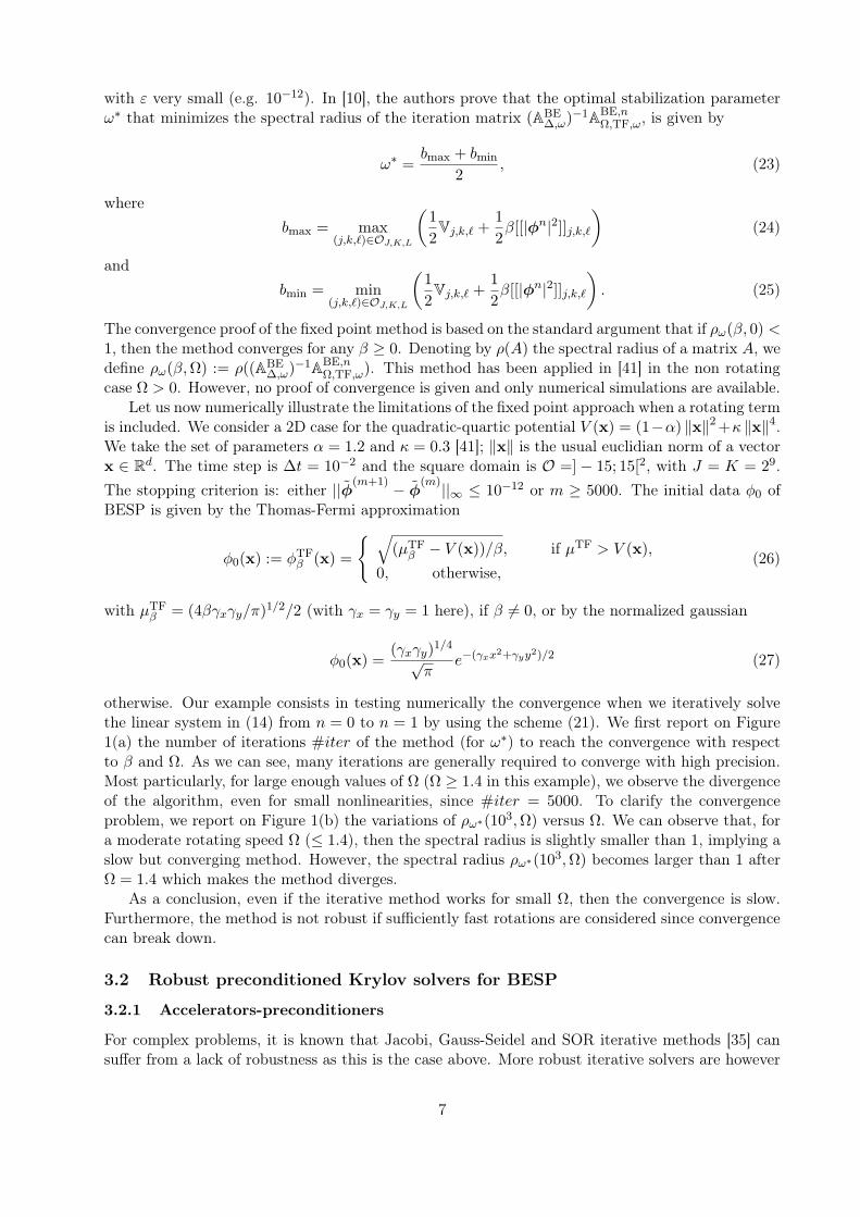
otherwise. Our example consists in testing numerically the convergence when we iteratively solvethe linear system in (14) from n = 0 to n = 1 by using the scheme (21). We first report on Figure1(a) the number of iterations #iter of the method (for ω∗) to reach the convergence with respectto β and Ω. As we can see, many iterations are generally required to converge with high precision.Most particularly, for large enough values of Ω (Ω ≥ 1.4 in this example), we observe the divergenceof the algorithm, even for small nonlinearities, since #iter = 5000. To clarify the convergenceproblem, we report on Figure 1(b) the variations of ρω∗(103,Ω) versus Ω. We can observe that, fora moderate rotating speed Ω (≤ 1.4), then the spectral radius is slightly smaller than 1, implying aslow but converging method. However, the spectral radius ρω∗(103,Ω) becomes larger than 1 afterΩ = 1.4 which makes the method diverges.

As a conclusion, even if the iterative method works for small Ω, then the convergence is slow.Furthermore, the method is not robust if sufficiently fast rotations are considered since convergencecan break down.

3.2 Robust preconditioned Krylov solvers for BESP

3.2.1 Accelerators-preconditioners

For complex problems, it is known that Jacobi, Gauss-Seidel and SOR iterative methods [35] cansuffer from a lack of robustness as this is the case above. More robust iterative solvers are however

7

200015001000β

500

00

0.2

0.4

0.6

0.8

1

1.2

1.4

1.6

1.8

2

Ω

1500

2000

2500

3000

3500

4000

4500

5000

(a) #iter vs. (β,Ω)

Ω

Spectr

al ra

diu

s

0 0.5 1 1.5 20.98

0.99

1

1.01

1.02

1.03

1.04

1.05

1.06

1.07

1.08

(b) ρω∗(103,Ω) vs. Ω

Figure 1: 2D quadratic-quartic potential: convergence/divergence of the iterative scheme (21) withrespect to Ω.

available like for example for Krylov subspace solvers [35]. These methods are well-adapted toefficiently solve large linear systems of the form

Aφ = b, (28)

where A is a matrix from MM (C) (a M ×M matrix with complex-valued coefficients) and b ∈CM . For example, successful solvers are the Conjugate Gradient Squared method (CGS) [35],the BiConjugate Gradient Stabilized method (BiCGStab) [35, 37] and the Generalized MinimalRESidual method (GMRES) [35, 36]. The two first methods rely on the minimization of the error(φ∗−φ(m))tA(φ∗−φ(m)), where φ∗ is the solution of system (28) and φ(m) is an approximation ofφ∗ in the Krylov subspace Km. These methods can be viewed as the minimization of a quadraticfunctional in terms of φ(m), using a ”search direction” and ”step length” method. The third methodis based on the minimization of the residual ‖Aφ(m) − b‖, for φ(m) ∈ Km, using the Arnoldiiteration. All these iterative methods are often called accelerators. If #iter is the number ofiterations to reach the solution with a required tolerance ε, then the global computational cost isgiven by Cglobal = #iter × Citer

A , where CiterA is the computational effort for one iteration. This is

directly related to the evaluation of matrix-vector products Ψ = Aψ, where ψ is given.The use of an accelerator alone is generally not sufficient [35]. Indeed, the convergence rate of

the solver e.g. #iter is guided by the way the eigenvalues of the operator spread out in the complexplane. Clustering is often an expected property to get fast convergence and a small number ofiterations to converge. This property cannot hold for the matrices arising in system (14) since theyare related to the discretization of second-order elliptic operators. To improve the convergence of thesolver and therefore to decrease #iter, one has to precondition the linear system. Preconditioners aregenerally built in an algebraic way as an approximation of the inverse of A in Eq. (28). Among themost robust preconditioners, let us for example mention ILUT methods, SPAI, multigrid techniques[35]. The restriction with these approaches is that they require the access to the entries of A. Inour case, this cannot be expected since the partial differential operators are efficiently evaluatedthrough FFTs (see Eq. (18)). An alternative is to rather approximate the original partial differentialoperator involved in the equation by another operator which can be easily inverted. We also have totake into account the computational cost of the application of such preconditioners into the globalscheme. For the BESP scheme, the operator that must be solved is given by

ABE,n =I

∆t− 1

2[[∆]]− ΩLz + V+ β[[|φn|2]]. (29)

8

When one wants to evaluate Ψ = ABE,nψ, for ψ ∈ CM , FFT/iFFTs must be used. Following [16],the computational cost of a FFT/iFFT for a complex-valued vector ψ is CFFT/iFFT = 5M log2(M).

Therefore, the evaluation of ABE,nψ requires one FFT and two iFFTs resulting in a global costCiterABE,n = 3CFFT for the application of the unpreconditioned operator.

A first possibility to precondition our system is to use the operator related to the fixed pointapproach. This results in the following preconditioned linear system to solve

(I+ PBE

∆ ABE,nΩ,TF

)φ = PBE

∆ bBE,n, (30)

where

PBE∆ =

(I

∆t− 1

2[[∆]]

)−1

and ABE,nΩ,TF = −ΩLz + V+ β[[|φn|2]]. (31)

In the sequel, the preconditioner ”PBE∆ ” is called ”Laplace” (∆) preconditioner and corresponds to

the discretization of the linear heat equation (diffusion part of the operator). Let us remark that amatrix-vector evaluation for the preconditioned operator equation has a global cost Citer

∆ = 4CFFT.A second simple preconditioner can be obtained by only keeping the explicit diagonal terms of

the original operator without partial differential operator to avoid any FFT computation and to getan explicit inversion. This gives us the second preconditioned system

(I+ P

BE,nTF ABE

∆,Ω

)φ = P

BE,nTF b

BE,n, (32)

where

PBE,nTF =

(I

∆t+ V+ β[[|φn|2]]

)−1

and ABE,n∆,Ω = −1

2[[∆]]− ΩLz. (33)

All along the paper, the preconditioner PBE,nTF is called ”Thomas-Fermi” (TF) preconditioner and is

associated with the BE discretization of the Thomas-Fermi equation without rotation. An analysisof the computational cost of a matrix-vector evaluation for this new equation shows that we obtain:Citer

TF = 3CFFT, which is the same as for the equation without preconditioner.

3.2.2 Numerical comparison of the preconditioned solvers for BESP

We first compare the different following accelerators: CGS, BiCGStab and GMRES without restart.The tolerance of the Krylov solvers is fixed to ε := 10−13 all along this section. We consider thesame situation and parameters as in subsection 3.1 for the fixed point approach. Let us chooseBiCGStab without preconditioner. We solve the BESP system to get the solution from n = 0to n = 1. We report on Figure 2(a) the number of iterations #iter vs. (β,Ω) for BiCGStab toconverge. Compared with the fixed point approach, we can first observe that the method alwaysconverges even for large Ω and is therefore robust. Furthermore, the number of iterations is alwaysmuch smaller than for the fixed point approach to get a very small residual and slightly grows withrespect to both increasing values of β and Ω. Hence, the method is efficient. We now compareon Figures 3 the efficiency of the Krylov solvers: GMRES, CGS and BiCGStab. We fix β = 2000and consider the same situation as above. We report the number of iterations #iter and the CPUtime (in seconds) required for the solver to converge. We can observe that the most efficient Krylovsolver is BiCGStab. For Ω = 0, CGS fails to converge, thus making it a non robust solver.

We now select the BiCGStab accelerator and compare the efficiency of the Laplace (∆-BiCGStab)and Thomas-Fermi (TF-BiCGStab) preconditioners for the same problem. As we can observe onFigure 4(a), the number of iterations #iter is strongly reduced when one considers the Thomas-Fermi preconditioner and is stable according to Ω. The effect of the Laplace preconditioner is lessimpressive most particularly for increasing values of Ω. The impact on the CPU time can be directlyseen on Figure 4(b).

9

200015001000β

500

00

0.2

0.4

0.6

0.8

1

1.2

1.4

1.6

1.8

2

Ω

50

60

70

80

90

100

110

120

130

(a) #iter vs. (β,Ω) for BICGStab without pre-conditioner to converge.

(b) Converged ground state for Ω = 2 and β =2000.

Figure 2: 2D quadratic-quartic potential: #iter vs. (β,Ω) for BiCGStab without preconditioner(left) and converged solution for β = 2000 (right).

Ω

#iter

0 0.2 0.4 0.6 0.8 1 1.2 1.4 1.6 1.8 290

100

110

120

130

140

150

160

170

180

BiCGStab

CGS

GMRES

(a) #iter vs. Ω

Ω

log

10(C

PU

tim

e(s

))

0 0.2 0.4 0.6 0.8 1 1.2 1.4 1.6 1.8 21.8

2

2.2

2.4

2.6

2.8

3

3.2

3.4

3.6

3.8

BiCGStab

CGS

GMRES

(b) log10(CPU time) vs. Ω

Figure 3: 2D quadratic-quartic potential: #iter (left) and log10 of the CPU time (right) vs. Ω forthe first time step of the Krylov solvers without preconditioner.

We now fix β = 2000 and Ω = 2. For computing the stationary solution, the global time stoppingcriterion is fixed (all along the paper) by

∥∥φn+1 − φn∥∥∞

≤ ǫ∆t, (34)

with ǫ = 10−6. According to (34), one obtains the computed ground state solution given on Figure2(b). We now solve the linear systems with and without preconditioner for the first 2 × 104 timesteps to see the behavior of the solvers over a long time interval. As we can see on Figure 5(a),the number of iterations per time step is strongly reduced all along the computations for the TF-BiCGStab solver. The preconditioner ∆-BiCGStab is also helpful but less effective. Furthermore,the reduction of iterations is quite stable over the time interval even if we can observe that lessiterations are needed for the first time steps (see Figure 5(b)).

We only retain TF-BiCGStab which has proved to be the most efficient and robust solver. Letus consider the computational domain O =] − 15, 15[2 with J = K = 29. The time step is fixedto ∆t = 10−2 and the stopping criterion for BiCGStab is given by formula (22) to ε = 10−6. Letus analyze the behavior of the preconditioned solver with respect to the nonlinearity strength β.

10

Ω

#iter

0 0.2 0.4 0.6 0.8 1 1.2 1.4 1.6 1.8 240

50

60

70

80

90

100

110

120

TF−BiCGStab

∆−BiCGStab

BiCGStab

(a) #iter vs. Ω

Ω

CP

U tim

e(s

)

0 0.2 0.4 0.6 0.8 1 1.2 1.4 1.6 1.8 240

50

60

70

80

90

100

110

120

130

TF−BiCGStab

∆−BiCGStab

BiCGStab

(b) CPU time vs. Ω

Figure 4: 2D quadratic-quartic potential: #iter (left) and CPU time (right) vs. Ω for the first timestep of BiCGStab with and without preconditioner.

Imaginary time

#iter

0 20 40 60 80 100 120 140 160 180 20020

40

60

80

100

120

140

TF−BiCGStab

∆−BiCGStab

BiCGStab

(a) #iter vs. imaginary time for 2× 104 time steps

Imaginary time

#iter

0 1 2 3 4 5 620

40

60

80

100

120

140

TF−BiCGStab

∆−BiCGStab

BiCGStab

(b) #iter vs. imaginary time for 6× 102 time steps

Figure 5: 2D quadratic-quartic potential: #iter for the first 2 × 104 time steps (left) and 6 × 102

time steps (right) vs. the imaginary time by using BiCGStab with and without preconditioner.

For Ω = 2, we consider five increasing values of β: 100, 500, 1000, 2000 and 5000. Figures 6report the number of iterations #iter with respect to the imaginary time for the first 104 timesteps. We observe that the convergence rate is not too strongly affected by the nonlinearity, evenfor large values of β. Only the first time steps show a different number of iterations according to theincreasing nonlinearity strength. We can conclude that the TF-BiCGStab preconditioner which isdesigned for strong nonlinear problems is indeed robust. Let us analyze the convergence propertieswith respect to the rotation speed Ω. We fix β = 2000 and consider Ω = 0, 1, 2, 3 and 3.5. As wecan see on Figures 7, the number of iterations increases with respect to Ω. This is due to the factthat the effect of the rotation is not included in the Thomas-Fermi preconditioner.

We now consider the influence of the time step ∆t on the total number of iterations needed toreach a ground state. We fix β = 300 and Ω = 0.5. We launch the BESP scheme for differentvalues of ∆t: 0.5, 0.1, 5 × 10−2, 10−2, 5 × 10−3, 10−3 and 5 × 10−4, for J = K = 29, a stoppingcriterion ε = 10−6 for BiCGStab and criterion (34) for the global iterative time scheme related tothe CNGF. As we can see on Figures 8, the total number of iterations to reach the same solutionis inversely proportional to the time step. An explanation to this phenomenon is that, when the

11

Imaginary time

#iter

0 10 20 30 40 50 60 70 80 90 10010

20

30

40

50

60

70

β = 100

β = 500

β = 1000

β = 2000

β = 5000

(a) #iter vs. imaginary time for 104 time steps

Imaginary time

#iter

0 0.5 1 1.5 2 2.5 315

20

25

30

35

40

45

50

55

60

65

β = 100

β = 500

β = 1000

β = 2000

β = 5000

(b) #iter vs. imaginary time for 3× 102 time steps

Figure 6: 2D quadratic-quartic potential and TF-BiCGStab: #iter vs. different values of β for thefirst 104 (left) and 300 (right) time steps (Ω = 2).

Imaginary time

#iter

0 10 20 30 40 50 60 70 80 90 1000

20

40

60

80

100

120

Ω = 0

Ω = 1

Ω = 2

Ω = 2.5

Ω = 3

(a) #iter vs. imaginary time for 104 time steps

Imaginary time

#iter

0 0.5 1 1.5 2 2.5 30

20

40

60

80

100

120

Ω = 0

Ω = 1

Ω = 2

Ω = 2.5

Ω = 3

(b) #iter vs. imaginary time for 3× 102 time steps

Figure 7: 2D quadratic-quartic potential and TF-BiCGStab: #iter vs. different values of therotation speed Ω for the first 104 (left) and 300 (right) time steps (β = 2000).

solution reaches an almost steady state, taking a larger time step is more adapted to attain theglobal minimum of the energy functional. However, in cases where the physical parameters β andΩ are larger, a smaller time step must be chosen since the minimization algorithm would otherwiseonly lead to a local minimum.

4 Three additional examples

From the previous section, we have seen that the TF-BiCGStab preconditioned solver is efficientand robust, most particularly for strong nonlinearities β, strong potentials and large rotation speedsΩ. We propose to investigate the properties of the preconditioned iterative solvers 1) for a problemwith a quadratic potential, 2) for a three-dimensional GPE and 3) for a two components BEC.

4.1 A problem with a harmonic potential

Here we consider the computation of the stationary state of the GPE with a quadratic potential:V (x) = 1

2‖x‖2 and a rotation speed ranging from 0 to 0.95 (1 is the critical velocity here). The

12

log10(∆t)

tota

l#iter

−3.5 −3 −2.5 −2 −1.5 −1 −0.5 0

×104

6

8

10

12

14

16

18

20

(a) #iter vs. ∆t

Imaginary time

#iter

0 50 100 150 200 250 300 3500

200

400

600

800

1000

1200

1400

1600

1800

∆ t = 0.5

∆ t = 0.1

∆ t = 0.05

∆ t = 0.01

∆ t = 0.005

∆ t = 0.001

∆ t = 0.0005

(b) #iter vs. imaginary time

Figure 8: 2D quadratic-quartic potential and TF-BiCGStab: total #iter vs. different time steps∆t (left) and #iter vs. imaginary time for a complete computation with different ∆t (right).

discretization/approximation parameters are the same as in subsection 3.1. First, let us considerBiCGStab with a tolerance ε equal to 10−13 and solve the BESP system from n = 0 to n = 1.The initial data is given by the Thomas-Fermi approximation (35) when β > 0. For β = 0, weconsider the normalized gaussian (36). From Figure 9(a), we can see that BiCGStab is robust andefficient. Additional numerical simulations show that the unpreconditioned CGS and BiCGStablead to about the same convergence rate and outperform GMRES. Let us fix β = 2000. On Figure9(b), we can see that, unlike the previous case, the Thomas-Fermi preconditioner does not reduce#iter while the Laplace preconditioner is extremely efficient. This reduction is furthermore almostnot affected by the value of Ω.

200015001000

β500

00

0.1

0.2

0.3

0.4

0.5

0.6

0.7

0.8

0.9

1

Ω

10

20

30

40

50

60

70

80

(a) #iter vs. (β,Ω) (without preconditioner)

Ω

#iter

0 0.1 0.2 0.3 0.4 0.5 0.6 0.7 0.8 0.9 10

10

20

30

40

50

60

70

80

TF−BiCGStab

∆−BiCGStab

BiCGStab

(b) #iter vs. Ω (with preconditioner)

Figure 9: 2D harmonic potential: #iter vs. (β,Ω) for BiCGStab without preconditioner (left) and#iter vs. Ω for the preconditioned BiCGStab (right).

4.2 A three-dimensional example

We consider now the 3D GPE Eq. (1) with potential V (x) = (1 − α)‖x‖2 + κ‖x‖4 (α = 1.2 andκ = 0.3). The time step is ∆t = 10−2 and the computational domain is ] − 30; 30[3, for a spatial

13

discretization with J = K = L = 27. The tolerance ε of the Krylov subspace solvers is 10−9 (allalong this section). The initial data φ0 for BESP is the Thomas-Fermi approximation

φTFβ (x) =

√(µTF

β − V (x))/β, if µTF > V (x),

0, otherwise,(35)

with µTFβ = (15βγxγyγz/(4π))

2/5/2 (with γx = γy = γz = 1 here), if β 6= 0, or the normalizedgaussian

φ0(x) =(γxγyγz)

1/4

π3/4e−(γxx2+γyy2+γzz2)/2 (36)

otherwise. We report on Figure 10 the number of iterations #iter vs. (β,Ω) for BiCGStab toconverge, from t0 = 0 to t1 = ∆t. Like the 2D case with quadratic-quartic potential, the method isrobust and efficient. Let us now compare the efficiency of the Krylov solvers: GMRES, CGS andBiCGStab. We fix β = 2000 and consider the same situation as above. We report on Figure 11(a)the number of iterations #iter to converge. We conclude that the most efficient solver is BiCGStab.We now analyze the performance of the preconditioned and unpreconditioned BiCGStab. As wecan see on Figure 11(b), the Thomas-Fermi preconditioner reduces a lot the number of iterations#iter. Moreover, this reduction is not affected by the value of Ω. In addition, the effect of theLaplace preconditioner does not provide such a reduction.

200015001000

β500

00

0.2

0.4

0.6

0.8

1

1.2

1.4

1.6

1.8

2

Ω

30

40

50

60

70

80

90

100

110

Figure 10: 3D quadratic-quartic potential: #iter vs. (β,Ω) for BICGStab without preconditionerto converge.

4.3 A two-components Bose-Einstein condensate

We consider now a two-components time-dependent GPE with rotating term and coupled nonlin-earities [8]

i∂tψ1(t,x) =

(−1

2∆ + V (x)−Ω · L

)ψ1(t,x) + βf1(|ψ1(t,x)|, |ψ2(t,x)|)ψ1(t,x)− ψ2(t,x),

i∂tψ2(t,x) =

(−1

2∆ + V (x)−Ω · L

)ψ2(t,x) + βf2(|ψ2(t,x)|, |ψ1(t,x)|)ψ2(t,x)− ψ1(t,x),

(37)for x ∈ Rd, t > 0. Functions ψ1 and ψ2 are the two components wave functions of the condensate.In our case, we have the following coupled nonlinearities [8]

f1(|ψ1(t,x)|, |ψ2(t,x)|) = β1,1|ψ1(t,x)|2 + β1,2|ψ2(t,x)|2

14

Ω

#iter

0 0.2 0.4 0.6 0.8 1 1.2 1.4 1.6 1.8 280

100

120

140

160

180

200

220

240

BiCGStab

CGS

GMRES

(a) #iter vs. Ω (without preconditioner)

Ω

#iter

0 0.2 0.4 0.6 0.8 1 1.2 1.4 1.6 1.8 20

20

40

60

80

100

120

TF−BiCGStab

∆−BiCGStab

BiCGStab

(b) #iter vs. Ω (with preconditioner)

Figure 11: 3D quadratic-quartic potential: #iter vs. Ω for the first time step of the Krylov solverswithout (left) and with (right) preconditioner.

andf2(|ψ2(t,x)|, |ψ1(t,x)|) = β2,2|ψ2(t,x)|2 + β2,1|ψ1(t,x)|2,

where β1,1 = 1, β2,2 = 0.97 and β1,2 = β2,1 = 0.94. Setting Ψ = (ψ1, ψ2), the energy of this systemis defined by

Eβ,Ω(Ψ) =

2∑

j=1

∫

Rd

1

2|∇ψj |2 + V (x)|ψj(x)|2 + β

βj,j2

|ψj |4 − Ωℜ(ψ∗jLzψj

)dx

+

∫

Rd

ββ1,2 + β2,1

2|ψ1(x)|2|ψ2(x)|2dx−

∫

Rd

2ℜ(ψ1(x)ψ2(x))dx. (38)

The mass conservation property writes down

||Ψ||20 =∫

Rd

(|ψ1(x)|2 + |ψ2(x)|2)dx = 1. (39)

To compute a stationary state of this system, we adapt the CNGF method [6, 8] which is energydiminishing. Being given a uniform time step ∆t = tn+1− tn, ∀n ∈ N, the CNGF formulation leadsto computing Φ = (φ1, φ2) solution to

∂tφ1 = −∇φ∗1Eβ,Ω(Φ) =

1

2∆φ1 − V φ1 − βf1(|φ1|, |φ2|)φ1 +ΩLzφ1 + φ2, tn < t < tn+1,

∂tφ2 = −∇φ∗2Eβ,Ω(Φ) =

1

2∆φ2 − V φ2 − βf2(|φ2|, |φ1|)φ2 +ΩLzφ2 + φ1, tn < t < tn+1,

Φ(x, tn+1) = Φ(x, t+n+1) =Φ(x, t−n+1)

||Φ(x, t−n+1)||0,

Φ(x, 0) = Φ0(x),x ∈ Rd, with ||Φ||0 = 1.

(40)

We assume that the two components evolve in O :=] − ax; ax[×] − ay; ay[×] − az; az[ (for the 3Dcase). Using the same notations as in the one-component case, the BESP scheme leads to solving

ABE,nΦ = b

BE,n,

Φn+1 =

Φ

||Φ||0,

(41)

15

where Φ = (φ1(xj,k,ℓ), φ2(xj,k,ℓ))(j,k,ℓ)∈OJ,K,Lis a discrete vector in C2M . If Φn

= (φn1 (xj,k,ℓ), φn2 (xj,k,ℓ))(j,k,ℓ)∈OJ,K,L

in C2M is an approximation of the solution Φ at time tn on the

spatial grid O, then the right hand side is given by bBE := Φ

n/∆t. The operator ABE,n is definedby the map which for any vector Φ = (φ1,φ2) ∈ C2M associates Ψ ∈ C2M such that

Ψ := ABE,nΦ = A

BE,nTF Φ+ ABE

∆,ΩΦ,

ABE,nTF Φ :=

(1

∆t

(I 00 I

)+

(V −1−1 V

)+ β

(F1(Φ

n) 00 F2(Φ

n)

))Φ,

ABE∆,ΩΦ :=

(−1

2

([[∆]] 00 [[∆]]

)− Ω

(Lz 00 Lz

))Φ,

(42)

where

F1(Φn) = β1,1[[|φn

1 |2]] + β1,2[[|φn2 |2]], F2(Φ

n) = β2,2[[|φn2 |2]] + β2,1[[|φn

1 |2]]. (43)

The operators above are evaluated by extending the strategy developed in the one-component case.Therefore, Krylov subspace solvers can be directly applied here. Concerning the preconditioners,the extension of the ”Laplace” preconditioner gives

PBE∆ =

(1

∆t

(I 00 I

)− 1

2

([[∆]] 00 [[∆]]

))−1

. (44)

For the ”Thomas-Fermi” preconditioner, we have the diagonal "Thomas-Fermi" preconditioner (TF-Diag in Figure 12(b))

PBE,nTF,Diag =

(1

∆t

(I 00 I

)+

(V 00 V

)+ β

(F1(Φ

n) 00 F2(Φ

n)

))−1

(45)

and the full ”Thomas-Fermi” (TF-Full in Figure 12(b)) preconditioner

PBE,nTF,Full =

(1

∆t

(I 00 I

)+

(V −1−1 V

)+ β

(F1(Φ

n) 00 F2(Φ

n)

))−1

. (46)

To analyze the algorithm, we consider the quadratic potential V (x) = 12 |x|2. In the CNGF, we

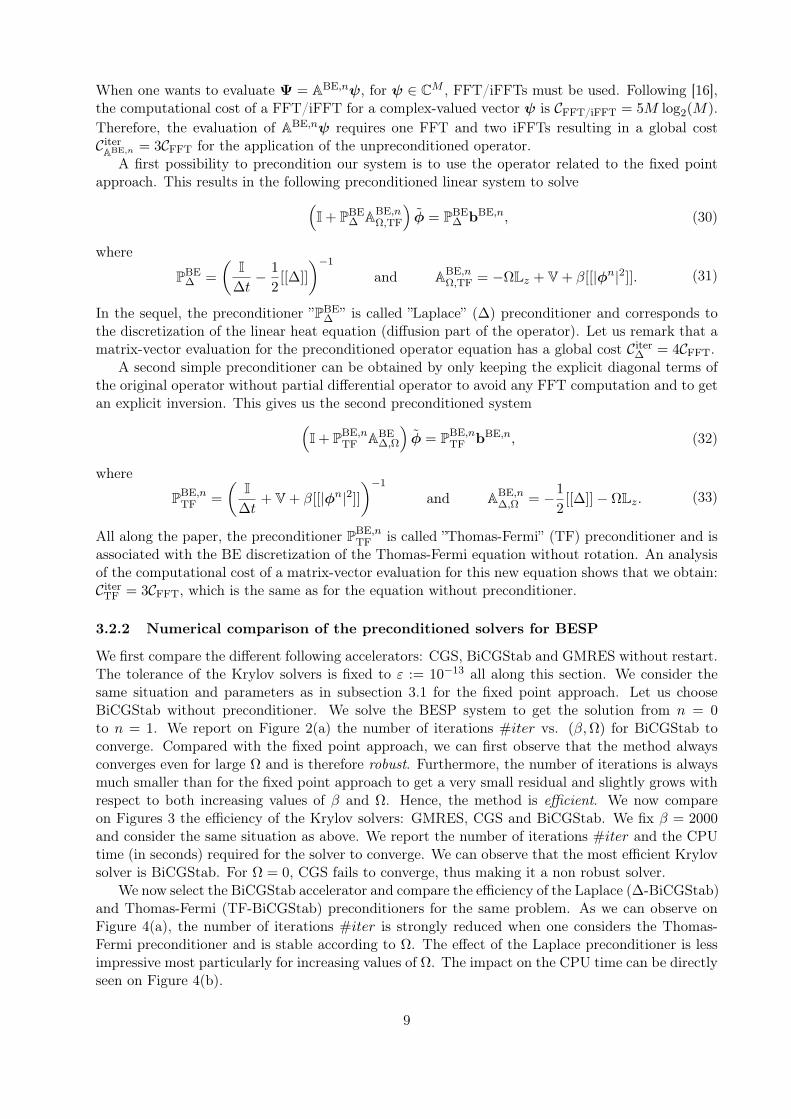
choose the time step ∆t = 10−2. The square domain is ]−15, 15[2, with J = K = 29. The toleranceε of the Krylov solvers is set to 10−13. The initial data Φ0 is: Φ0 = (φ0, φ0), where φ0 is eithergiven by the Thomas-Fermi approximation (35) when β > 0, or by the normalized gaussian (36)when β = 0. On Figure 12(a), we report the number of iterations #iter vs. (β,Ω) for BiCGStab toconverge, (steps n = 0 to n = 1). Like in the one-component case (see Section 4.1), we observe thatBiCGStab is robust and efficient. Extensive numerical simulations show that BiCGStab has thebest convergence rate compared to GMRES and CGS while being robust. Let us fix β = 2000. Wereport on Figure 12(b) #iter for the different preconditioned BiCGStab. We see that the ”Laplace”preconditioner leads to the best performance. There is no gain when considering the diagonal andfull TF preconditioners.

5 GPELab: an associated Matlab toolbox

The methods presented in the paper are the basic methods implemented in the freely availableGross-Pitaevskii Equation Laboratory∗ (GPELab) Matlab toolbox. The aim of this collection ofalgorithms is in particular to compute ground states of multi-components BECs with rotating terms

∗http://www.iecn.u-nancy.fr/~duboscq/GPELab.html

16

200015001000

β500

00

0.1

0.2

0.3

0.4

0.5

0.6

0.7

0.8

0.9

1

Ω

10

20

30

40

50

60

70

80

(a) #iter vs. Ω (without preconditioner)

Ω

#iter

0 0.1 0.2 0.3 0.4 0.5 0.6 0.7 0.8 0.9 120

30

40

50

60

70

80

90

100

TF−Diag−BiCGStab

TF−Full−BiCGStab

∆−BiCGStab

BiCGStab

(b) #iter vs. Ω (with preconditioner)

Figure 12: 2D harmonic potential for the 2-components case: #iter vs. (β,Ω) for BiCGStab(without preconditioner) and #iter vs. Ω for the preconditioned BiCGStab (right) to converge.

and general nonlinearities based on the preconditioned BESP scheme. Therefore, all the test casesreported here can be directly reproduced by using the associated Matlab scripts [5]. Furthermore,GPELab allows to compute the (stochastic) dynamics of BECs based on GPEs by using a ReSP[15] or second- and fourth-orders time splitting spectral schemes [8, 11] (that are explicit and so donot need any linear system solution).

6 Conclusion

We presented an accurate, efficient and robust method based on BESP for computing the stationarystates of strongly nonlinear and fast rotating GPEs. The method combines a Backward Eulerscheme in time and FFT-based discretization in space. The associated linear systems are solved bythe BiCGStab solver in conjunction with a Laplace or Thomas-Fermi preconditioner. The method issupported by a full numerical study with various one- and two-components examples in 2D and 3D.Finally, an associated Matlab code, GPELab [5], can be freely downloaded for testing the methodfor a large class of problems related to the GPE.

Considering a Relaxation scheme, we can also extend [28] the method for computing the dy-namics of vortices [4, 42]. It appears that the preconditioned CGS is the most robust and efficientiterative method in the case of the ReSP scheme.

Acknowledgements. This work was partially supported by the French ANR grants MicroWaveNT09_460489 (”Programme Blanc” call) and ANR-12-MONU-0007-02 BECASIM (”Modèles Nu-mériques” call).

References

[1] J.R. Abo-Shaeer, C. Raman, J.M. Vogels, and W. Ketterle, Observation of vortex lattices inBose-Einstein condensates, Science 292 (2001), no. 5516, 476–479.

[2] S.K. Adhikari, Numerical solution of the two-dimensional Gross-Pitaevskii equation for trappedinteracting atoms, Physics Letters A 265 (2000), no. 1-2, 91–96.

17

[3] M.H. Anderson, J.R. Ensher, M.R. Matthews, C.E. Wieman, and E.A. Cornell, Observation ofBose-Einstein condensation in a dilute atomic vapor, Science 269 (1995), no. 5221, 198–201.

[4] X. Antoine, W. Bao, and C. Besse, Computational methods for the dynamics of the nonlin-ear Schrodinger/Gross-Pitaevskii equations, to appear in Computer Physics Communications(http://dx.doi.org/10.1016/j.cpc.2013.07.012).

[5] X. Antoine and R. Duboscq, GPELab: A Matlab toolbox for computing stationary solutionsand dynamics of Gross-Pitaevskii Equations (GPE), User-guide, (2013), http://www.iecn.

u-nancy.fr/~duboscq/downloads/GPELab_Documentation.pdf.

[6] W. Bao, Ground states and dynamics of multi-component Bose-Einstein condensates, Multi-scale Modeling and Simulation: A SIAM Interdisciplinary Journal 2 (2004), no. 2, 210–236.

[7] W. Bao and Y. Cai, Ground states of two-component Bose-Einstein condensates with an inter-nal atomic Josephson junction, East Asian Journal on Applied Mathematics 1 (2011), 49–81.

[8] , Mathematical theory and numerical methods for Bose-Einstein condensation, Kineticand Related Models 6 (2013), no. 1, 1–135.

[9] W. Bao, Y. Cai, and H. Wang, Efficient numerical methods for computing ground states anddynamics of dipolar Bose-Einstein condensates, Journal of Computational Physics 229 (2010),no. , 7874–7892.

[10] W. Bao, I.L. Chern, and F.Y. Lim, Efficient and spectrally accurate numerical methods for com-puting ground and first excited states in Bose-Einstein condensates, Journal of ComputationalPhysics 219 (2006), no. 2, 836–854.

[11] W. Bao and H. Wang, An efficient and spectrally accurate numerical method for computingdynamics of rotating Bose-Einstein condensates, Journal of Computational Physics 217 (2006),no. 2, 612–626.

[12] W.Z. Bao and Q. Du, Computing the ground state solution of Bose-Einstein condensates by anormalized gradient flow, SIAM Journal on Scientific Computing 25 (2004), no. 5, 1674–1697.

[13] W.Z. Bao and W.J. Tang, Ground-state solution of Bose-Einstein condensate by directly min-imizing the energy functional, Journal of Computational Physics 187 (2003), no. 1, 230–254.

[14] D. Baye and J.M. Sparenberg, Resolution of the Gross-Pitaevskii equation with the imaginary-time method on a Lagrange mesh, Physical Review E 82 (2010), no. 5, 2.

[15] C. Besse, A relaxation scheme for the nonlinear Schrödinger equation, SIAM Journal on Nu-merical Analysis 42 (2004), no. 3, 934–952.

[16] J.P. Boyd, Chebyshev and Fourier Spectral Methods, Second edition, Dover, New York, 2001.

[17] C.C. Bradley, C.A. Sackett, J.J. Tollett, and R.G. Hulet, Evidence of Bose-Einstein conden-sation in an atomic gas with attractive interactions, Physical Review Letters 75 (1995), no. 9,1687–1690.

[18] V. Bretin, S. Stock, Y. Seurin, and J. Dalibard, Fast rotation of a Bose-Einstein condensate,Physical Review Letters 92 (2004), no. 5.

[19] M. Caliari, A. Ostermann, S. Rainer, and M. Thalhammer, A minimisation approach for com-puting the ground state of Gross-Pitaevskii systems, Journal of Computational Physics 228

(2009), no. 2, 349–360.

18

[20] M. Caliari and S. Rainer, GSGPEs: A MATLAB code for computing the ground state of systemsof Gross-Pitaevskii equations, Computer Physics Communications 184 (2013), no. 3, 812–823.

[21] M.M. Cerimele, M.L. Chiofalo, F. Pistella, S. Succi, and M.P. Tosi, Numerical solution of theGross-Pitaevskii equation using an explicit finite-difference scheme: An application to trappedBose-Einstein condensates, Physical Review E 62 (2000), no. 1, B, 1382–1389.

[22] M.L. Chiofalo, S. Succi, and M.P. Tosi, Ground state of trapped interacting Bose-Einsteincondensates by an explicit imaginary-time algorithm, Physical Review E 62 (2000), no. 5, B,7438–7444.

[23] F. Dalfovo, S. Giorgini, L.P. Pitaevskii, and S. Stringari, Theory of Bose-Einstein condensationin trapped gases, Review of Modern Physics 71 (1999), no. 3, 463–512.

[24] I. Danaila and F. Hecht, A finite element method with mesh adaptivity for computing vor-tex states in fast-rotating Bose-Einstein condensates, Journal of Computational Physics 229

(2010), no. 19, 6946–6960.

[25] I. Danaila and P. Kazemi, A new Sobolev gradient method for direct minimization fo the Gross-Pitaevskii energy with rotation, SIAM Journal on Scientific Computing 32 (2010), no. 5, 2447–2467.

[26] K.B. David, M.O. Mewes, M.R. Andrews, N.J. Vandruten, D.S. Durfee, D.M. Kurn, andW. Ketterle, Bose-Einstein Condensation in gas of sodium atoms, Physical Review Letters75 (1995), no. 22, 3969–3973.

[27] C.M. Dion and E. Cances, Ground state of the time-independent Gross-Pitaevskii equation,Computer Physics Communications 177 (2007), no. 10, 787–798.

[28] R. Duboscq, Analyse et Simulation d’Equations de Schrödinger Déterministes et Stochastiques.Applications aux Condensats de Bose-Einstein en Rotation, Ph.D. Thesis, Université de Lor-raine, to appear, 2013.

[29] M. Edwards and K. Burnett, Numerical solution of the nonlinear Schrödinger equation forsmall samples of trapped neutral atoms , Physical Review A 51 (1995), no. 2, 1382–1386.

[30] A. Gammal, T. Frederico, and L. Tomio, Improved numerical approach for the time-independentGross-Pitaevskii nonlinear Schrödinger equation, Physical Review E 60 (1999), no. 2, B, 2421–2424.

[31] K.W. Madison, F. Chevy, V. Bretin, and J. Dalibard, Stationary states of a rotating Bose-Einstein condensate: Routes to vortex nucleation, Physical Review Letters 86 (2001), no. 20,4443–4446.

[32] K.W. Madison, F. Chevy, W. Wohlleben, and J. Dalibard, Vortex formation in a stirred Bose-Einstein condensate, Physical Review Letters 84 (2000), no. 5, 806–809.

[33] M.R. Matthews, B.P. Anderson, P.C. Haljan, D.S. Hall, C.E. Wieman, and E.A. Cornell,Vortices in a Bose-Einstein condensate, Physical Review Letters 83 (1999), no. 13, 2498–2501.

[34] C. Raman, J.R. Abo-Shaeer, J.M. Vogels, K. Xu, and W. Ketterle, Vortex nucleation in astirred Bose-Einstein condensate, Physical Review Letters 87 (2001), no. 21.

[35] Y. Saad, Iterative Methods for Sparse Linear Systems, SIAM, 2nd edition, 2003.

19

[36] Y. Saad and M.H. Schultz, GMRES - a Generalized Minimal RESidual algorithm for solvingnonsymmetric linear systems, SIAM Journal on Scientific and Statistical Computing 7 (1986),no. 3, 856–869.

[37] H.A. Van Der Vost, BI-CGSTAB - a fast and smoothly converging variant of BI-CG for thesolution of nonsymmetric linear systems , SIAM Journal on Scientific and Statistical Computing13 (1992), no. 2, 631–644.

[38] Y.-S. Wang and C.-S. Chien, A spectral-Galerkin continuation method using Chebyshev poly-nomials for the numerical solutions of the Gross-Pitaevskii equation, Journal of computationaland applied mathematics 235 (2011), no. 8, 2740–2757.

[39] Y.-S. Wang, B.-W. Jeng, and C.-S. Chien, A two-parameter continuation method for rotatingtwo-component Bose-Einstein condensates in optical lattices, Communications in Computa-tional Physics 13 (2013), 442–460.

[40] C. Yuce and Z. Oztas, Off-axis vortex in a rotating dipolar Bose-Einstein condensate, Journalof Physics B-Atomic Molecular and Optical Physics 43 (2010), no. 13.

[41] R. Zeng and Y. Zhang, Efficiently computing vortex lattices in rapid rotating Bose-Einsteincondensates, Computer Physics Communications 180 (2009), no. 6, 854–860.

[42] Y. Zhang, Numerical Study of Vortex Interactions in Bose-Einstein Condensation, Communi-cations in Computational Physics 8 (2010), 327–350.

20