rm e steeldesign ec

RM Bridge Professional Engineering Software for Bridges of all Types

RM Bridge V8i

December 2012

COMPOSITE BRIDGE – STEEL DESIGN EC

RM Bridge

C o m p o s i t e B r i d g e – S t e e l D e s i g n E C

© Bentley Systems Austria

Copyright

This document is integral part of the program package RM Bridge. Duplication and dissemi-

nation is only allowed with explicit permission of Bentley Systems or authorised agents.

© 2012, Bentley Systems, Incorporated. All Rights Reserved

http://www.bentley.com/

RM Bridge Contents

Composite Bridge – Steel Design EC I


Contents

1 Introduction ..................................................................................................................... 1-1

1.1 Background .............................................................................................................. 1-1

1.2 General Description ................................................................................................. 1-1

2 Structural Data ................................................................................................................. 2-2

2.1 General Layout ........................................................................................................ 2-2

2.2 Numbering Scheme ................................................................................................. 2-3

2.3 Support Conditions .................................................................................................. 2-4

2.4 Main Girders ............................................................................................................ 2-5

2.4.1 Definition of the Main Girder Segments ............................................................. 2-6

2.5 Cross Frames and Stiffeners .................................................................................... 2-7

2.6 Materials ................................................................................................................ 2-10

3 Construction Schedule and Loading .............................................................................. 3-11

3.1 Element Activation by Stages ............................................................................... 3-11

3.2 Design Loads ......................................................................................................... 3-13

3.2.1 Dead Load.......................................................................................................... 3-13

3.2.2 Live loads .......................................................................................................... 3-13

3.2.3 Braking Load ..................................................................................................... 3-14

3.2.4 Wind Loads ....................................................................................................... 3-14

3.2.5 Thermal Forces .................................................................................................. 3-15

3.3 Load Combinations ............................................................................................... 3-15

4 Analysis results .............................................................................................................. 4-18

5 Steel Design Checks ...................................................................................................... 5-22

5.1 General................................................................................................................... 5-22

5.2 Slender parts .......................................................................................................... 5-22

5.2.1 Definition of Slender parts ................................................................................ 5-23

5.2.2 Slender parts in the current example ................................................................. 5-24

5.3 Buckling lengths .................................................................................................... 5-24

5.3.1 Definition of Buckling Lengths ......................................................................... 5-25

RM Bridge Contents

Composite Bridge – Steel Design EC II


5.3.2 Buckling Lengths in the current example .......................................................... 5-26

5.4 Design Resistances (without considering locked-in stressing).............................. 5-27

5.4.1 General............................................................................................................... 5-27

5.4.2 Main girders – Typical sections......................................................................... 5-27

5.4.3 RM Bridge Results ............................................................................................ 5-33

5.4.4 Assessments ........................................................................................................ 5-35

5.5 Capacity Factors ...................................................................................................... 5-35

5.5.1 Definitions ........................................................................................................... 5-35

5.5.2 Resulting Capacity factors ................................................................................. 5-36

5.6 Consideration of locked-in stresses ....................................................................... 5-36

RM Bridge Introduction

Composite Bridge – Steel Design EC 1-1


1 Introduction

1.1 Background

This training and demonstration example is used to show the application of RmBridge on a

composite bridge with concrete slab and welded I-girders as main girders. This example is

also used as a verification example for the RM Bridge functionality for steel design in accord-

ance with Eurocode EN 1993 (steel structures) and EN 1994 (composite structures). The same

example has also been used by the French company Sétra in their “Guidance book, Eurocodes

3 and 4, Application to steel-concrete composite road bridges”.

The respective hand-calculation results of this Guidance Book have been used as a reference

for comparison with and verification of the RmBridge results.

1.2 General Description

The bridge is a continuous road bridge with 3 spans and 2 welded I-shaped main girders. The

roadway has 2 traffic lanes with 3.5 m width and lateral strips of 2 m on each side.

The analyses comprise Static analysis for loads prescribed in Eurocode EN 1991-2, calcula-

tion of Design Resistances for all girders and actual steel checks comparing ULS loads with

resistances.

Figure 1-1: General view of the RM model

RM Bridge Structural Data



2 Structural Data

The bridge is a continuous road bridge with 3 spans and 2 welded I-shaped main girders. The

roadway has 2 traffic lanes with 3.5 m width, and lateral strips of 2 m on each side.

Figure 2-1 : Schematic view of the cross-section

Summary of cross-section data:

Total slab width 12.0 m

Spacing of main girders 7.0 m

Overhang left and right 2.5 m

Effective depth of concrete slab 0.307 m

Effective haunch depth 0.109 m

Depth of steel girders 2.8 m

Upper flange width 1.0 m

Lower flange width 1.2 m

2.1 General Layout

The structure is modelled as a grillage with two axes in the longitudinal direction and four

axes in the transverse direction (one for each of the cross-members at the beginning and the

end of the system (A1, A2) as well as over the piers (P1, P2)). Each of these 6 axes has its

own associated segment.




Figure 2-2: Span distribution

The longitudinal overhang at begin and end of the bridge is assumed 0.8 m.

The model has been prepared with the wizard functionality of RM Bridge, which allows for an

easy and straightforward definition of the structure. However, model preparation could also

be done directly in the standard RM Bridge GUI.

In plan the structure is straight and abutments and piers are orthogonal to the longitudinal di-

rection of the superstructure. The piers are drop cap piers with bearings under each main gird-

er of the superstructure.

Default pier dimensions of the wizard have been used without consideration of actual feasibil-

ity, as the focus of this example is just on superstructure design and not on substructure de-

sign.

Longitudinal fixation is assumed at the left abutment, bearings over the piers and the right

abutment are assumed free to move in longitudinal direction.

2.2 Numbering Scheme

The bridge wizard automatically creates nodes and elements of the structural system and the

respective node and element numbers.

Due to modeling the structure as a girder grid we have two main girders, left (MG1) and right

(MG2). Both main girders are composite girders, where structural elements are assigned to the

individual cross-section parts as well as to the full composite section.

The actual refinement of the calculation model is automatically done by the wizard. Default

(and minimum) subdivision is 24 per span, i.e. with considering the left and right overhang

the first and the last span will have 25 elements, and the intermediate spans will have 24 ele-

ments with equal length.

If there are additional points of interest in the system, this regular subdivision will be auto-

matically adapted. The wizard considers every point, where the cross-section of a main girder

changes, as additional point of interest. I.e. points, where a parameter of the cross-section

changes (e.g. web thickness or flange thickness) the program automatically places a subdivi-




sion point. It depends on the distance of such a point from the regular subdivision points

whether a new point is inserted or the nearest regular point is moved into this position.

Note that the program does not check the actual change of a cross-section parameter, but just

whether there is a constraint point in the variation diagram. I.e. the user may enforce the pro-

gram to create a subdivision point at a certain position by assigning a Variation to one param-

eter (e.g. the web width) and specifying the value in this position no matter whether the value

before or behind this point is the same.

Note also that the program does not automatically create additional subdivision points at posi-

tions of cross-frames, bracings or stiffeners. Those are always eccentrically connected to the

nearest subdivision point on the main girder. If the user wants to have subdivision points at

the positions of cross-frames, he must place at this position a variation constraint point as ex-

plained above.

In our example we have in the first and last span a cross-frame distance of 7.5 m which is 1/8

of the the span length. I.e. cross-frame positions automatically coincide with regular subdivis-

tion points. However, in the center span we have cross-frame distances of 8.0 m (1/10 of the

span length). Therefore, in order to have subdivision points in these positions, we defined

respective variation constraint points in the variation of the web thickness (see variation

tw_S02 in the wizard). As a consequence, we have in the center span 30 elements in longitu-

dinal direction instead of 24.

Table 2-1: Numbering scheme

Item Span 1 Span 2 Span3

Node numbers (MG1) 101-125 201-230 301-325

Element numbers (MG1, steel) 10101-10125 10201-10230 10301-10325

Element numbers (MG1, concrete) 20101-20125 20201-20230 20301-20325

Element numbers (MG1, composite) 101-125 201-230 301-325

Node numbers (MG2) 401-425 501-530 601-625

Element numbers (MG2, steel) 10401-10425 10501-15230 10601-10625

Element numbers (MG1, concrete) 20401-20425 20501-20530 20601-20625

Element numbers (MG1, composite) 401-425 501-530 601-625

Abutments/Piers (left) 80001, 80002 80003-80025 80027-80049

Abutments/Piers (right) 80003-80025 80027-80049 80051, 80052

2.3 Support Conditions

The following table defines the support conditions in reference to the local coordinate system

of the spring elements (alpha1 = 90 degrees), i.e. X = vertical, Y = longitudinal, Z = trans-

verse direction. Actual stiffness of bearings and foundation is not considered and spring con-

stant 1e+008 indicates a rigid support.

Table 2-2: Support conditions

Axis Part/Soil Elem Type C-X C-Y C-Z C-MX C-MY C-MZ

Abut-

ment 1

1

2

80001

80002

Spring

Spring

1e+008 1e+008 1e+008

1e+008 1e+008 1e+008

Pier 1 1

2

Soil

80009

80010

80012

Spring

Spring

Spring

1e+008 1e+008

1e+008

1e+008 1e+008 1e+008 1e+008 1e+008 1e+008




Soil

Soil

80017

80022

Spring

Spring

1e+008 1e+008 1e+008 1e+008 1e+008 1e+008

1e+008 1e+008 1e+008 1e+008 1e+008 1e+008

Pier 2 1

2

Soil

Soil

Soil

80033

80034

80036

80041

80046

Spring

Spring

Spring

Spring

Spring

1e+008 1e+008

1e+008

1e+008 1e+008 1e+008 1e+008 1e+008 1e+008

1e+008 1e+008 1e+008 1e+008 1e+008 1e+008

1e+008 1e+008 1e+008 1e+008 1e+008 1e+008

Abut-

ment 2

1

2

80051

80052

Spring

Spring

1e+008 1e+008

1e+008

2.4 Main Girders

Every main girder has a constant depth of 2800 mm and the variations in thickness of the up-

per and lower flanges are found towards the inside of the girder. The lower flange is 1200 mm

wide whereas the upper flange is 1000 mm wide.

Figure 2-3: Structural steel distribution for Upper and Lower main girder flanges




Figure 2-4: Structural steel distribution of the main girder web

2.4.1 Definition of the Main Girder Segments

Separate segments are created by the wizard for each span and each main girder

(w1_Span01.01, w1_Span01.02, w1_Span02.01, w1_Span02.02, w1_Span03.01,

w1_Span03.02). Creating the model in the RM Bridge Modeler would of course also allow

working with 2 segments reaching over all spans. In the first and last span the segments are

subdivided into 25 elements with typical element length of 2.5 m. In the center span we have

30 elements with a typical length of 2.667 m, but some variation of the element length (2.0 m,

3.0 m) to meet the relevant points where cross-frames are connected or the cross-section var-

ies.

The main girder segment numbering systems are given in chapter 2.2 (Numbering Scheme). A

cross section must be assigned to every segment point. Cross-section w1_Deck is assigned to

the span part of the first main girder and the same w1_Deck for the second main girder.

Figure 2-5: Segmentation of the 3rd

span




Figure 2-6: w1_Deck cross-section

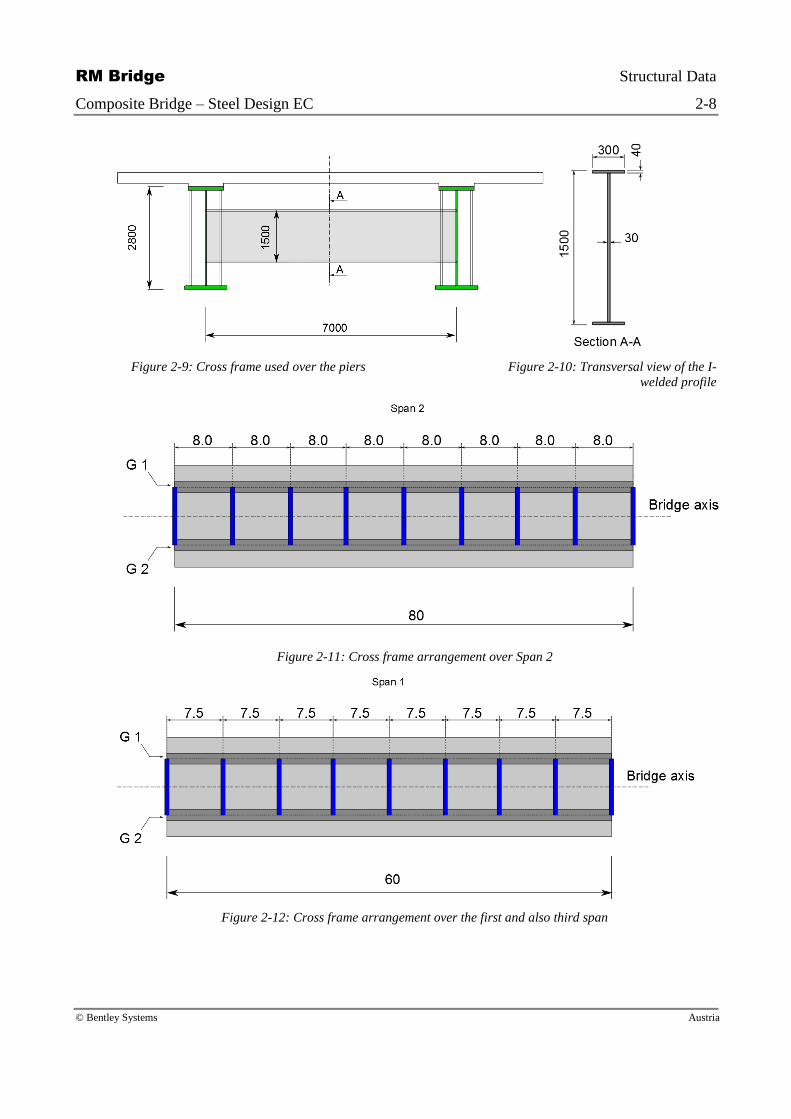
2.5 Cross Frames and Stiffeners

Steel cross frames are arranged over the piers and in the spans. Over the piers we have a

welded I girder with height of 1.5 m and 30 cm wide flanges. Cross frames in span are rolled I

beams IPE-600.

Figure 2-7: Cross frame used in the span Figure 2-8: Transversal view of theIPE 600

profile




Figure 2-9: Cross frame used over the piers Figure 2-10: Transversal view of the I-

welded profile

Figure 2-11: Cross frame arrangement over Span 2

Figure 2-12: Cross frame arrangement over the first and also third span




At each cross frame position stiffeners are present on both sides of the main girder.

Figure 2-13: T-welded profile used for transverse stiffneres

Diaphragm elements are numbered as follows:

Over the left abutment Element 50001

Over the first pier Element 50091

Over the second pier Element 50191

Over the right abutment E lement 50261

Cross frames in span have a spacing of 7.5 m in the first and last span, respectively 8 m in the

central span. The numbering is:

Left Span Elements 50001 to 50081 step 10

Central Span Elements 50091 to 50181 step 10

Right Span Elements 50191 to 50261 step 10

Slab reinforcement:

For both reinforcing steel layers, the transverse reinforcing bars are placed outside the longi-

tudinal reinforcing bars, on the side of the slab free surface.

Transverse reinforcing steel

At mid-span of the slab (between the main steel girders)

o High bond bars with diameter Φ = 20 mm, spacing s = 170 mm in upper layer

o High bond bars with diameter Φ = 25 mm, spacing s = 170 mm in lower layer

In the slab sections supported by the main steel girders



Longitudinal reinforcing steel

In span

o High bond bars with diameter Φ = 16 mm, spacing s = 130 mm in upper and

lower layers (i.e. in total ρs = 0, 92% of the concrete section)

In intermediate support regions:



o (i.e. in total ρs = 1, 19% of the concrete section)




Figure 2-14: Location of mid-span and support sections for longitudinal reinforcement

Figure 2-15: Green lines representing longitudinal reinforcement in w1_deck Cross section

2.6 Materials

Reinforcement: St_500(A)

o Yield Strength: 500000 kN/m2

o Modulus of Elasticity: 200E+06 kN/m2

Concrete: Type C 35/45

o Compressive Strength: 37000 kN/m2


Structural Steel: S355 (members with less than 40 mm thickness)



Structural Steel: S355_t40 (members with more than 40 mm thickness)



RM Bridge Construction Schedule and Loading



3 Construction Schedule and Loading

Stage-wise erection is only related to subsequent erection of superstructure, bearings, steel

construction and concrete slab, but there are assumed that all spans are erected simultaneously

(erection of the whole steel construction in one stage, pouring the whole slab in one stage).

3.1 Element Activation by Stages

Each construction stage is related to a certain active system, which may contain all elements

of the model or just a part of them. The activation of new elements is done in Schedule >

Stages > Activation. Elements, which already have been activated in previous construction

stages remain active until they are explicitly deactivated, and must not be specified again in a

subsequent stage. An appropriate indication is given by the program in the case that a previ-

ously activated element is again specified. If the user then selects the option <Overwrite>, the

element will be removed from the previous construction stage and added in the current stage.

The activation of the elements in the different stages is shown below.

Stage SubS

Activation of earth springs and pier elements:

80003-80008; 80012-80015; 80017-80020; 80022-80025; 80027-80032; 80036-

80039; 80041-80044; 80046-80049.

Stage Abutment

Activation of left and right bearings

80001-80002; 80009-80010; 80033-80034; 80051-80052.

Stage Girder

Activation of steel girders including cross-frames, bracings and stiffeners

Main girders: 10101-10125; 10201-10230; 10301-10325; 10401-10425; 10501-

10530; 10601-10625

Cross-frames: 50001-50261

Lateral bracings: 60001-60351

Vertical Stiffeners: 70001-70261; 70401-70661




Figure 3-1: Active structure after installing main and secondary steel members

Stage Slab

Activate concrete elements, shear studs and composite elements

Composite elements: 101-125; 201-230; 301-325; 401-425; 501-530; 601-625

Concrete slab elements: 20101-20125; 20201-20230; 20301-20325; 20401-20425;

20501-20530; 20601-20625

Shear studs: 30101-30125; 30201-30230; 30301-30325; 30401-30425; 30501-

30530; 30601-30625

Further Stages

All further stages in the schedule don’t contain new activations but are just defined to group

the different categories of actions.




3.2 Design Loads

3.2.1 Dead Load

Self-weight (concrete): 25 kN/m3

Self-weight (steel): 78.5 kN/m3

Additional dead load (asphalt, traffic barriers...): 15.0 kN/m each main girder

3.2.2 Live loads

The traffic load is applied according to EC 1991-2, 4 and currently considers Load Model 1

(LM1) consisting of a concentrated load (Tandem-System TS) and uniformly distributed loads

(UDL). UDL and TS from load model LM1 are positioned longitudinally and transversally on

the deck so as to achieve the most unfavorable effect for the studied main girder.

When the position of the load trains is between two girders then the program automatically

calculates the distribution to the both girders. The wizard arranges the traffic lanes tightly

from left to right resulting in maximum influence to the left girder. (Note that the left girder is

the bottom girder in plan, because in cross-section presentation we always look in negative

longitudinal direction). If the mirror option is selected, the program also investigates the ar-

rangement from right to left to get also the worst influence for the right girder. This is the de-

fault selection also used in this example.

Figure 3-2: Traffic loading on the bridge

TS (Tandem system):

Axle distance: 1.2 m

Load intensity 1st lane 270 kN per axle

Load intensity 2nd

lane 160 kN per axle

Load intensity 3rd

lane 80 kN per axle

UDL (distributed load):




Load intensity 1st lane 18.9 kN/m

Load intensity other lanes 7.5 kN/m

Load intensity rest area 7.5 kN/m

The factor for the tandem-system is 0.9; The UDL on the notional lanes is 0.7 and the UDL

on the remaining area is 1.0.

3.2.3 Braking Load

The braking load is calculated according to EC 1991-2, 4.4.

The load is considered to be applied uniformly distributed in longitudinal direction along the

roadway axis acting at the finished roadway level and in case of grillage modeling distributed

proportionally to all applicable main girders.

There is no influence line evaluation made for the braking load, but the whole braking load is

applied in one loadcase w1_brake as distributed load over the whole roadway surface. The

total line load intensity is calculated and then distributed to the different girders.

Total braking load 832.32 kN

Height of application 0.3m above cross-section surface

Length of the bridge 201.6 m

Line load intensity 4.129 (= 832.32/201.6)

3.2.4 Wind Loads

Figure 3-3: Wind loading on the bridge

The wind load is calculated according to EC 1991-1-4, 8.

Air density ρ 1.25 kg/m3

(= 0.00125 t/m3)

Design wind speed vb with traffic 23 m/s

Design wind speed vb without traffic 32 m/s

Wind pressure with traffic 1.0254 kN/m2




Wind pressure without traffic 1.984 kN/m2

Attack area (height) with traffic 5.216 m

Attack area (height) without traffic 3.816 m

Vertical component of wind pressure (see EN1991-1, 8.3.3)

For both upward and downward wind the eccentricity e of the application point of the vertical

wind force from the center line of the cross-section is 3 m.

The default wind load factor C for the vertical wind load is considered 0.9 (see EN 1991-1,

8.3.3 (1)).

Calculated area load of vertical wind pressure; 0.576 KN/m2.

3.2.5 Thermal Forces

Uniform temperature load:

The default value of the initial temperature is considered by T0=10 °C, Te,min=-20 , Te,max=41

ΔTN,neg = Te,min – T0 -30°

ΔTN,pos = Te,max – T0 +31°

RM calculates 2 load cases w1_T-const1 (ΔTN,pos) and w1_T-const2 (ΔTN,neg). Both load cases

are based on a load set with unit load 1.0° C, which is factorized by the relevant ΔT value.

Linear temperature gradient:

EC also requires investigating a gradient of the temperature over the depth of superstructure.

This gradient may be assumed linear. However, many other design codes require a non-linear

gradient be considered. Therefore we use in the program the more general TempVar approach

which is based on temperature points along the vertical centerline of the cross-section.

The design gradients are defined in the code in terms of temperature differences between top

and bottom surface. They are

+15° (positive value - top temperature greater than bottom temperature)

-18° (negative value – top temperature smaller than bottom temperature)

The gradient as specified in the code is internally transformed into an equivalent top tempera-

ture and bottom temperature in accordance with the position of the COG. These values are

used in the reference sets describing the temperature distribution over the cross-section depth.

3.3 Load Combinations

RM Bridge offers the possibility of defining a combination table describing the rules for au-

tomatic load case superposition and creation of result envelopes. Templates for automatic

generation of this combination table are available for many design codes. Also, the wizards

automatically generate the relevant combination table for the selected design code. The com-

bination table for Eurocode as used in this example is shown below in Figure 3-4. It is a very

comprehensive table, but only few generated envelopes are used in this example.




Figure 3-4: Combination table for Eurocode

Abstract of predefined Load Combinations (EN 1991-2):

SLS - Combinations I to VI - "Characteristic combinations"

Comb. I, IV: Pm, t=0, t=∞

Comb. II, V: Pk, t=0

Comb. III, VI: Pk, t=∞

SLS - Combination VII and VIII - "Frequent combinations"

Comb. VII: Pk, t=0

Comb. VIII: Pk, t=∞

SLS - Combinations IX to X - "Quasi-permanent combinations"

Comb. IX: Pk, t=0

Comb. X: Pk, t=∞




ULS - Combinations XI and XIII - "Fundamental combinations"

Comb. XI: gr1 group is comprised in this example from vertical uniformly distributed

loads and vertical concentrated loads from Load Model 1.

Comb.XII: n addition to gr1 we consider the wind action.

Comb. XIII: gr2 group is comprised of braking and acceleration forces

ULS - Combination XIV - "Seismic combination"

Comb. XIV – Design combination for seismic design (not used in this example)

Wind and Braking loadings are not mentioned in the Setra documentation, but for complete-

ness of the generated model they are treated here.

RM Bridge Analysis results



4 Analysis results

Figures below illustrate a few results of internal forces and moments coming from the global

analysis of the deck in the design example.

All diagrams below are related to the first main girder MG1. Due to the symmetry conditions

there is no difference between the 2 girders and assessing just 1 of them is sufficient.

Figure 4-1 below shows the extreme bending moments of the main girder due to traffic. The

comparison with the Setra results as shown in Figure 4-2 shows.

Referring now to the ultimate state design moments presented in Figure 4-3, we see that max-

imum hogging moments are about 106200 kNm and the maximum positive moment in the

center is about 52300 kNm. Due to the fact that the Setra analysis considered cracking of the

slab over the pier, we expect that our hogging moment will be slightly higher and maximum

positive moment will be slightly lower. Indeed the reported values in the Setra document

(Figure 4-4) meet these expectations.

Shear forces (Figure 4-5 and Figure 4-6): The maximum value of the shear-force over the

piers is some +- 8000 kN. When we compare this with the results given in the Setra document

we see maxima of some 7450 kN, i.e. we have a difference of some 7% which can be accept-

ed considering that slightly different assumptions have been used in the Setra analysis.

Figure 4-1: Moments for traffic loads (UDL and TS) – RM results




Figure 4-2: Moments for traffic loads (UDL and TS) - Setra document

Figure 4-3: Moments of final ULS (comb. 11) and characteristic SLS (comb.6) combinations – RM results




Figure 4-4: Moments of final ULS (comb. 11) and characteristic SLS (comb.6) combinations - Setra document

Values of final ULS envelope match very well.

Figure 4-5: Shear forces for ULS (comb. 11) and characteristic SLS (comb. 6) combinations – RM results




Figure 4-6: Shear forces for ULS (comb. 11) and characteristic SLS (comb. 6) combinations – Setra document

Figure 4-7: Vertical displacement (Vy) from ULS actions

RM Bridge Steel Design Checks



5 Steel Design Checks

5.1 General

Steel design checks in RM Bridge are performed in 2 steps:

1. Calculation of design resistances (Schedule action UltRes)

2. Actual proof check using interaction formulas (Schedule action ResChk)

The relevant design resistances can be stored in superposition files like normal impact enve-

lopes. This allows viewing them in the GUI in the same way than viewing structural analysis

results, with the full functionality of graphic presentation.

Plotting the resistances into the same diagram together with the relevant ULS combination

allows for direct graphical assessment of the results as shown in Figure 5-6 and Figure 5-7.

Note that the calculation of basic resistances without consideration of locked-in force effects

is based on the presumption of sufficient stress redistribution capacity by plasticization. I.e. in

theory this is only allowed for class 1 and 2 cross-sections. These resistances must be com-

pared with so called “Joined forces”, i.e. fictitious internal forces on the composite section

which are equivalent to the combined effect of forces acting on the steel girders only (self

weight, wet concrete) and forces acting on the composite section (SDL, traffic, …).

RM Bridge also allows taking locked-in forced into account by specifying the load case con-

taining the relevant forces acting on the steel part only. In that case the capacity factor is re-

lated to the additional forces acting on the composite section. These results are described in

chapter 5.6, “Consideration of locked-in stresses”.

2nd

additional input parameter sets must be specified to be able to perform steel checks:

1. The definition of “Slender cross section parts” to check for local buckling phenomena

in the cross section plane (buckling of cross-section plates), and

2. The definition of characteristic lengths (buckling lengths) for buckling phenomena in

longitudinal direction of the members.

5.2 Slender parts

The definition of slender cross-section parts (SP) is required to consider local buckling phe-

nomena due to compression forces. These slender parts are defined as lines between two

points of the cross-section, with the thickness t as additional parameter. These slender parts

are used for the cross-section classification as described in the next section.

The characteristic slenderness value used for classification is the width to thickness ratio, de-

fined as c/t in Eurocode or slenderness parameter λ in AASHTO code. The thickness is com-

monly denoted t, often with reference to the type of the part (tw for web, tf for flange). Differ-

ent rules are given in the different design codes for defining the relevant width of slender

parts.




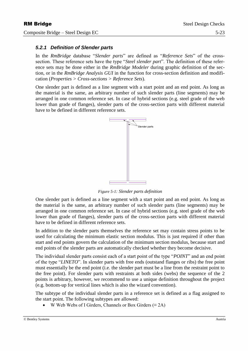
5.2.1 Definition of Slender parts

In the RmBridge database “Slender parts” are defined as “Reference Sets” of the cross-

section. These reference sets have the type “Steel slender part”. The definition of these refer-

ence sets may be done either in the RmBridge Modeler during graphic definition of the sec-

tion, or in the RmBridge Analysis GUI in the function for cross-section definition and modifi-

cation (Properties > Cross-sections > Reference Sets).

One slender part is defined as a line segment with a start point and an end point. As long as

the material is the same, an arbitrary number of such slender parts (line segments) may be

arranged in one common reference set. In case of hybrid sections (e.g. steel grade of the web

lower than grade of flanges), slender parts of the cross-section parts with different material

have to be defined in different reference sets.

Figure 5-1: Slender parts definition

One slender part is defined as a line segment with a start point and an end point. As long as

the material is the same, an arbitrary number of such slender parts (line segments) may be

arranged in one common reference set. In case of hybrid sections (e.g. steel grade of the web

lower than grade of flanges), slender parts of the cross-section parts with different material

have to be defined in different reference sets.

In addition to the slender parts themselves the reference set may contain stress points to be

used for calculating the minimum elastic section modulus. This is just required if other than

start and end points govern the calculation of the minimum section modulus, because start and

end points of the slender parts are automatically checked whether they become decisive.

The individual slender parts consist each of a start point of the type “POINT” and an end point

of the type “LINETO”. In slender parts with free ends (outstand flanges or ribs) the free point

must essentially be the end point (i.e. the slender part must be a line from the restraint point to

the free point). For slender parts with restraints at both sides (webs) the sequence of the 2

points is arbitrary, however, we recommend to use a unique definition throughout the project

(e.g. bottom-up for vertical lines which is also the wizard convention).

The subtype of the individual slender parts in a reference set is defined as a flag assigned to

the start point. The following subtypes are allowed:

W Web Webs of I Girders, Channels or Box Girders (≡ 2A)




F Flange Outstand Flanges of I Girders, T-Girders, Channels, etc. (≡ 1A)

B Box Flanges of box girders (restraint on both sides) (≡ 2B)

R Rib Outstand rib e.g. stems of T girders, ribs or stiffeners (≡ 1B)

Like the subtype, the effective thickness of the slender part is also a parameter assigned to the

start point. For calculating the slenderness of the part the program calculates the length of the

line between the start and end point and divides it by the effective thickness.

5.2.2 Slender parts in the current example

In our example we use SlenderF and SlenderW as reference sets in definition of the main

girders, and SlenderF and SlenderR in the definition of secondary members (cross frames and

stiffeners).

Figure 5-2: Slender parts definition in the Cross section.

5.3 Buckling lengths

The characteristic length for local buckling of main girders is in general defined by the rele-

vant distance of transverse stiffeners. The characteristic length for lateral-torsional buckling is

normally the distance between cross-frames or diaphragms. Buckling due to normal force is




not relevant for the main girder; nevertheless reasonable values for the respective buckling

lengths have been defined (automatically created by the wizard).

5.3.1 Definition of Buckling Lengths

As a theoretical and accurate calculation of these characteristic lengths is impossible, they are

directly defined for the different beams elements in the GUI in Structure > Elements > Buck-

ling lengths. Separate values can be defined for the start point and the end point of each ele-

ment.

The characteristic length for local buckling of main girders is in general defined by the rele-

vant distance of transverse stiffeners. The characteristic length for lateral-torsional buckling is

normally the distance between cross-frames or diaphragms.

The RmBridge wizard functionality automatically creates this table of characteristic lengths in

accordance with above habits with the following constitutive law for standard I girder compo-

site bridges:

Steel main girders (constructability check):

L-rz Span length respectively overhang length at begin and end

L-ry Cross frame distance

L-rx Cross-frame distance

L-loc Distance of transverse stiffeners

L-lt Distance of transverse stiffeners

Composite main girders (ULS check):

L-rz Span length respectively overhang length at begin and end

L-ry Zero

L-rx Zero

L-loc Distance of transverse stiffeners

L-lt Distance of transverse stiffeners

Cross-frame members and diaphragms

L-rz = L-ry = Lrx = L-loc = L-lt = nominal member length

These characteristic lengths may also be directly defined in the GUI in Structure > Elements

> Buckling lengths. It is also possible to define separate values start points and end points of

the different elements. The following defaults are valid if not all lengths are specified:

No buckling lengths L-rz, L-ry, L-rx defined: the program assumes that there is

no flexural and no torsional-flexural buckling hazard

Only L-rz defined: the program assumes L-ry and L-rx the same (one com-

mon beam buckling length)

No L-loc defined: the program assumes that there are no transverse stiffeners

No L-lt defined: the program assumes there is no lateral-torsional buckling

hazard




5.3.2 Buckling Lengths in the current example

Table 5-1

L-rx Elements L-ry L-rz L-loc L-lt

0.8 101 0.8 0.8 0.8 0.8

7.5 102-125 7.5 60.0 7.5 7.5

8.0 201-230 8.0 80.0 8.0 8.0

7.5 301-324 7.5 60.0 7.5 7.5

0.8 325 0.8 0.8 0.8 0.8

0.8 401 0.8 0.8 0.8 0.8

7.5 402-425 7.5 60.0 7.5 7.5

8.0 501-530 8.0 80.0 8.0 8.0

7.5 601-624 7.5 60.0 7.5 7.5

0.8 625 0.8 0.8 0.8 0.8

0.8 10101 0.8 0.8 0.8 0.8

7.5 10102-10125 7.5 60.0 7.5 7.5

8.0 10201-10230 8.0 80.0 8.0 8.0

7.5 10301-10324 7.5 60.0 7.5 7.5

0.8 10325 0.8 0.8 0.8 0.8

0.8 10401 0.8 0.8 0.8 0.8

7.5 10402-10425 7.5 60.0 7.5 7.5

8.0 10501-10530 8.0 80.0 8.0 8.0

7.5 10601-10624 7.5 60.0 7.5 7.5

0.8 10625 0.8 0.8 0.8 0.8




5.4 Design Resistances (without considering locked-in stressing)

5.4.1 General

In RM Bridge design resistances for slender steel and composite sections are calculated in the

schedule action UltRes. The calculated resistance values are written into a listfile and an Ex-

cel sheet, and also stored in a superposition file in order to allow for subsequently using

standard result presentation techniques for graphic presentation of design resistances.

In composite sections where we may have locked-in stresses due to stage-wise assembly of

the whole section, the resistances may either be calculated without considering locked-in

stresses or – by specifying the relevant locked-in stressing state (load case) – as additional

resistances (forces which can be applied on the composite section in addition to the locked-in

forces in the individual elements).

In order to distinguish between the 2 situations in composite elements we speak of “total”

resistances if locked-in stresses are not considered and of “additional” resistances if they are

considered. The “total” resistances must be compared with the joined ULS forces, i.e. we as-

sume that in the ultimate state the locked-in stresses will be redistributed to the composite

section. Note that the “total” resistances are not correct for slender cross-section, because lo-

cal buckling failure will occur before redistribution due to plasticization can take place.

5.4.2 Main girders – Typical sections

RM Bridge calculates the resistances for all element start and end points with the respective

switch in the element table set to “Yes”. This allows presenting diagrams along the bridge as

shown in Figure 5-6: Bending resistances and ULS bending moments along the main gird-

erand Figure 5-7: Shear resistances and ULS shear forces along the main girder. Only re-

sistances for bending moments Mz and shear forces My are shown here, because these are the

design relevant quantities.

For comparison a hand-calculation is made for 2 typical sections:

the cross-section over the piers (element 125), and

the cross-section in the center of center span (span 2, element 215)

5.4.2.1 Hand calculation for a Cross Section over Pier1: element 125

Bending Resistance +z (positive moment in Span)

Cross Section is in class 1




Figure 5-3: P .N.A in top flange (Flange_top)

Assumption: pna in Flange_top

Table 5-2

e = 0.5089

A_pl F=A_pl*335000/1 Dist.to pna F Dist to pna M_pl

Reinf_top 0.0188 6304.348 e – 0.073 0.436 2748.696

Reinf_bot 0.0120 4034.783 e – 0.263 0.246 992.557

Concrete 0.1066 35700.950 e – 0.150 0.359 12816.641

Haunch 0.0069 2301.450 e – 0.358 0.151 347.519

Flange_top_t 1*(e-0.4160) [.. ] * 335000 (e– 0.416)/2 31121.500 0.046 1431.589

Flange_top_b 1*(0.5360-e) [ ..] * 335000 (0.536 – e)/2 9078.500 0.014 127.099

Web 0.0660 22123.400 1.806 – e 1.297 28694.050

Flange_bot 0.1440 48240.000 3.136 – e 2.627 126726.480

top 79463.031 18337.002

bot 79441.900 155547.629

F_top = F_bot: 6304.348 + 4034.783 + 35700.950 + 2301.450 + (e –0.416) * 335000 = (0.536

– e) * 335000 + 22123.400 + 48240.000 => e = 0.5089

h_top = M_top / F = 0.2308

h_bot = M_bot / F = 1.9580 => a = h_top + h_bot = 2.1888

M_pl = F * a = 173928.682 bending plastic resistance +z

W_pl = M_pl / fy = 0.519 plastic section modulus

Bending Resistance –z




Cross Section is in class 2

Figure 5-4:P.N.A in Web

Assumption: pna in Web

Table 5-3

e = 1 .676

A_pl F=A_pl*335000/1 Dist to pna F Dist to pna M_pl

Reinf_top 0.0188 6304.348 e – 0.073 1.603 10105.870

Reinf_bot 0.0120 4034.783 e – 0.263 1.413 5701.148

Flange_top 0.12 40200.000 e – 0.476 1.200 48240.00

Web_t 0.026*e – 0.014 [.. ] * 335000 0.5*e– 0.268 9907.960 0.570 5647.537

Web_b 0.080-0.026*e [ ..] * 335000 -0.5*e+1.538 12202.040 0,700 8541.428

Flange_bot 0.1440 48240.000 3.136 – e 1,460 70430.400

top 60447.091 69694.555

bot 60442.040 78971.828

F_top = F_bot: 6304.348 + 4034.783 + 40200.000 + (0.026 * e – 0.014) * 335000 =

= (0.080 + 0.026 * e) * 335000 + 48240 => e = 1.676

h_top = M_top / F = 1.153

h_bot = M_bot / F = 1.307 => a = h_top + h_bot = 2.460

M_pl = F * a = 148699.844 bending plastic resistance -z




W_pl = M_pl / fy = 0.444 plastic section modulus

To be noticed that the program uses the same yield strengths fy=335000 for the entire length

of the bridge an so we will get a bigger bending resistance over the pier than normally in prac-

tice were for plate thicknesses t>100 mm fy=295000 which will reduce the bending resistance

over the pier region.

5.4.2.2 Hand calculation for a Cross Section at mid span P1-P2: element 215

w1_Deck:015:3 of Element 215 => COMPOSITE

Bending Resistance +z

fck = 35000.000

Table 5-4

Design plastic resistance of concrete in compression

Fc = Ac*0.85*fck/γc=6*0.307*0.85*35000/1.5=36530

Design plastic resistance of upper flange

Ffs =Afs*Fyf/ γm0 =1*0.04*335000=13400

Design plastic resistance of the bottom flange

Ffi =Afi*Fyf/ γm0 =1.2*0.04*335000=16080

Design plastic resistance of the web

Ffw =Aw*Fyw/ γm0=2.72*0.018*335000= 16401.6

Total = 45881.6

dimensions c t c/t Dist. Epsilon Class Area Gamma

bottom flange 0.6 0.04 15 2799.98 0.837552 1 0.048 1

web 2.72 0.018 151.1111 2798.6 0.837552 4 0.04896 1

upper flange 0.5 0.04 12.5 0.4435 0.837552 1 0.04 1

slab 0 0.307 0 0.1535 Total: 0.13696 1.5

haunch 0 0.109 0 0.3615 1.5

reinforcement top 0 0.07 144 1.15

bottom reinforcement 0 0.07 92.79 1.15




Fc+Ffs>Ffi+Fw

P.N.A located in structural upper flange X= 13.95313433 mm

Class 2 cross section and determine normal plastic moment resistance of the cross-section

Plastic verification EUROCODE EN 1994-2 5.5.2(3)

Figure 5-5: Design plastic resistance moment of the flanges only

Mpl,rd= 0.436*13400+1.816*16401.6+3.196*16080=87019.386 bending resistance +z




w1_Deck:021:2 of Element 10125=> Shear Resistance in y – direction for cross section

fy = 335000 ( authoritative yield ) ; Ay_Shear = 0.071 ; γ 0 =1.000;γ 1 =1.100

Vpl_rd = Ay_Shear * fy / ( 3 * γ) =13769.22 plastic shear resistance

Reduction required? L / t >= 72 * ε /η with η = 1.2 for steel grades <= 460

97.682 >= 50.250 => yes

a = infinite; λw = hw / (86.4 * t * ε) with hw = 2.54; t = 0.026 => λw = 1.350

λw > 0.83 / η => 1.350 > 0.692 =>

χ w = 0.83 / λw = 0.615 … reduction factor

k τ = 5.340 ; σ E = 190 000 000 * t^2 / h^2 = 19908.240

Vpl, rd_res = Vpl, rd* χ w* γ 0/ γ 1=13769.22*0.615*1.0/1.1=7698.246 reduced plastic

shear resistance

Shear Resistance in y – direction for beam

Vpl_rd=13769.22 plastic shear resistance

L-loc is defined => a = 8.000

Reduction required? L/t >= 72 * ε /η with η = 1.2 for steel grades <= 460

97.682 >= 50.250 => yes

a / b = L-loc / hw = 8.000 / 2.540 = 3.150 > 1 => k τ = 5.34 + 4.00 * ( b / a )^2 =

5.743

λw = hw / ( 37.4 * t * ε * k τ ) with hw = 2.54 ; t = 0.026 => λw = 1,301

λw > 0.83 / η => 1.301 > 0.692 =>χ w = 0.83 / λw = 0.638 … reduction factor

Vpl, rd_res = Vpl, rd* χ w* γ 0/ γ 1=13769.22*0.638*1.0/1.1=7696.148 reduced plastic

shear resistance




5.4.3 RM Bridge Results

The following table shows a summary of the calculated bending resistance values for the

composite section over pier 1 (begin of element 201) and in the centre of span 2 (begin of

element 214) to be compared with the above hand-calculated values. The full development of

resistances along the bridge is shown in the subsequent Figure 5-6: Bending resistances and

ULS bending moments along the main girderand Figure 5-7: Shear resistances and ULS shear

forces along the main girder.

The table contains the relevant resistance values together with additional eccentricities of the

normal force, if the effective cross-section has been changed for accounting for local buckling

hazard. For lateral torsional buckling only the negative moment is relevant (bottom flange in

compression) as the top flange is laterally fixed by the concrete plate. I.e. lateral torsional

buckling needs not be considered in the centre span. No reduction for lateral torsional buck-

ling is applied in element 201.

Table 5-5: Element resistence table

Elem N+ My+ Mz+ ey+ ez+ N- My-

201 119764.6 24668.02 174974.1 0.0 0.0 -98200.2 - 24668

Mz- ey- ez- Mx Qy Qz

-147871.6 0.0 0.0 0.0 7983.5 41496

Elem N+ My+ Mz+ ey+ ez+ N- My-

214 52941.6 4789 79463.1 0.0 0.0 -50753.2 -4789

Mz- ey- ez- Mx Qy Qz

-50166.8 0.0 0.0 0.0 3588.9 13887.9




Figure 5-6: Bending resistances and ULS bending moments along the main girder

Figure 5-7: Shear resistances and ULS shear forces along the main girder




5.4.4 Assessments

Figure 5-6 shows that the bending resistance is sufficient throughout the whole girder length.

Resistance values are in the relevant points typically 30-50 % higher than required.

However, as can be seen in Figure 5-7, shear resistance is not everywhere sufficient, i.e. the

thicker web should be arranged over a wider region over the piers and also near the abut-

ments, if there are no additional vertical stiffeners arranged.

5.5 Capacity Factors

5.5.1 Definitions

Capacity factors are utilization levels describing the utilization of the resistance of a cross-

section under the design loading. They will be greater than 1.0 when the generalized re-

sistance is less than the generalized impact.

The definition and calculation of these capacity factors is based on the respective formulas

required for verification of mixed impact and given in the design codes:

(E.g. EN 1993-1-1, 6.2.1(7)): NEd/NRd + My, Ed/My, Rd + Mz, Ed/Mz, Rd ≤ 1

RM Bridge allows for calculating different capacity factors relating to individual internal

force components or to a mixed impact.

For normal force and bending we have the following capacity factors:

CN = NEd / Nt,Rd or NEd / Nc,Rd Capacity factor for normal force

CMy = My,Ed / My+,Rd or My,Ed / My-,Rd Capacity factor for My

CMz = Mz,Ed / Mz+,Rd or Mz,Ed / Mz-,Rd Capacity factor for Mz

C2d,y = NEd/NRd + My,Ed/My,Rd Capacity factor for combination N + My

C2d,z = NEd/NRd + Mz,Ed/Mz,Rd Capacity factor for combination N + Mz

C3d = NEd/NRd + My, Ed/My, Rd + Mz, Ed/Mz, Rd Capacity factor for the full vector N + My +Mz




5.5.2 Resulting Capacity factors

Figure 5-8: Girder 1 composite section capacity factors

5.6 Consideration of locked-in stresses

Calculation of resistances due to locked–in stress

w1_Deck:007, Elements 402 and 10402

LC SUM-SW as locked-in

stress

N / Mx My / Mz Qy / Qz

10402 (single steel) -29.20/85.56 -19.63 / -50.92 -1198.29 / 24.91

402 (joined composite) 29.20/-274.79 -29.14 / -86.03 -1198.29 / 24.91

Class Mz-, N 4




Composite CS Resistance BucklingResistance Remaining Resistance

Mz+ 63.100 79463.100 79549.131

Mz- 166.890 Calculated via

fy_eff

Calculated via

fy_eff

Qy 3443.974 3608.338 2409.438 / +4807.238

Nc -76991.512 Calculated via

fy_eff

Calculatedvia fy_eff

Nt 52941.643 Calculated via

fy_eff

Calculated via fy_eff

Nc_remaining calculated via fy_eff

Relevant stresspoint: SlenderF:SLP05:2 (SLP06)

y_steel = ey_steel – y_stpt = -1.896 + 3.196 = 0.5; z_steel = ez_steel – z_stpt = 0 – 0.6 = 0.6

fyc = -335000 ; E = 2.1E8 ; Iz_steel = 0.009095 ; Iy_steel = 0.1973 ; Aeff_steel = 0.096,

Ac_comp = 0.230

chi_steel = 0.751

eps = N_steel / E / Aeff_steel + Mz_steel / E / Iz_steel * y_steel + My_steel / E / Iy_steel *

z_steel = -0.00000923

=>fy_eff = fyc * chi_steel – E * eps = -251585.000 + 1938.300 = -249646.700

Nc_comp = fyc * Ac_comp = -77050

Nc_b_comp = fy_eff * Ac_comp = -57418.741




Nt_remaining calculated via fy_eff

Relevant stresspoint: SlenderF:SLP01:2 (SLP02)

y_steel = ey_steel – y_stpt = -1.896 + 0.436 = -1.460; z_steel = ez_steel – z_stpt = 0 – 0.5 = -

0.5

fyt = 335000 ; E = 2.1E8 ; Iz_steel = 0.009095 ; Iy_steel = 0.1973 ; Aeff_steel = 0.096,

At_comp = 0.158

chi_steel = 1.000 (no buckling hazard for tension)


z_steel = 0.000005485

=>fy_eff = fyt * chi_steel – E * eps = 335000 – 1151.800 = 333848.200

Nt_comp = fyt * At_comp = 52930.000

Nt_b_comp = fy_eff * At_comp = 52748.016

Mz-_remaining calculated via fy_eff

Relevant stresspoint: SlenderF: SLP05:2 (SLP06);

y_steel = ey_steel – y_stpt = -1.896 + 3.196 = 1.3; z_steel = ez_steel – z_stpt = 0 + 0.6 = 0.6

fy = +/-335000 ; E_comp = 2.1E8 ; Iz_steel = 0.1973 ; Ax_steel = 0.13716

chi_steel = 1.000; y_steel > 0 => compression => fy = -335000


z_steel = -0.00000878

=>fy_eff = fy * chi_steel – E * eps = -335000 + 1843.38 = -333156.603

y_comp = ey_eff_comp_iter1 – y_stpt = -0.557 + 3.196 = 2.639

kappa = fy_eff / E / y_comp = -0.00060116

Izeff_comp_iter1 = 0.395175

Mz-_comp = kappa0 * E_comp * Izeff_comp_iter1 = -49888.264




Figure 5-9: Normal force resistance due to locked in stresses on composite section

Figure 5-10: Bending moment resistance due to locked in stresses on composite section




Figure 5-11: Shear resistances due to locked in stresses on composite section

rm e steeldesign ec

Documents

types rm bridge v8i

program package rm bridge

design loads

dead load

braking load

load combinations

live loads

wind loads