risk transfer and foreclosure law: evidence from the
TRANSCRIPT

Risk Transfer and Foreclosure Law: Evidence from the
Securitization Market∗
Danny McGowan†and Huyen Nguyen‡
September 24, 2019
Abstract
We evaluate the effect of foreclosure law on mortgage securitization and interest rates.
Exploiting exogenous variation in foreclosure law along US state borders using a regres-
sion discontinuity design, we find lenders are 4% more likely to securitize GSE-eligible
mortgages but do not differentiate interest rates when subject to borrower-friendly
foreclosure law. For non-GSE-eligible loans, foreclosure law does not affect securitiza-
tion but causes a 7 basis points increase in interest rates. The results highlight how
the GSEs’ common interest rate policy inhibits risk-based pricing, increases the GSEs’
debt holdings, and exposes taxpayers to the housing market.
JEL-Codes: G21, G28, K11.
Keywords: foreclosure law, GSEs, securitization, mortgage guarantees
∗We are grateful for helpful comments from Adolfo Barajas, Christa Bouwman, Ralph Chami, Pi-otr Danisewicz, Hans Degryse, Bob DeYoung, Ronel Elul, Iftekhar Hasan, Dasol Kim, Michael Koetter,Elena Loutskina, Mike Mariathasan, William Megginson, Klaas Mulier, Enrico Onali, Fotios Pasiouras,Amiyatosh Purnanandam, George Pennacchi, Klaus Schaeck, Glenn Schepens, Koen Schoor, ChristopheSpaenjers, Armine Tarazi, Jerome Vandenbussche and seminar and conference participants at Bangor,Birmingham, Durham, the EFI Research Network, the Financial Intermediation Research Society, theFINEST Spring Workshop, FMA Europe, the IMF, IWH-Halle, Leeds, Limoges, Loughborough, Notting-ham, and the Western Economic Association.†University of Birmingham. Email: [email protected]‡University of Bristol. Email: [email protected]
1
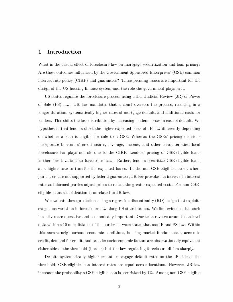
1 Introduction
What is the casual effect of foreclosure law on mortgage securitization and loan pricing?
Are these outcomes influenced by the Government Sponsored Enterprises’ (GSE) common
interest rate policy (CIRP) and guarantees? These pressing issues are important for the
design of the US housing finance system and the role the government plays in it.
US states regulate the foreclosure process using either Judicial Review (JR) or Power
of Sale (PS) law. JR law mandates that a court oversees the process, resulting in a
longer duration, systematically higher rates of mortgage default, and additional costs for
lenders. This shifts the loss distribution by increasing lenders’ losses in case of default. We
hypothesize that lenders offset the higher expected costs of JR law differently depending
on whether a loan is eligible for sale to a GSE. Whereas the GSEs’ pricing decisions
incorporate borrowers’ credit scores, leverage, income, and other characteristics, local
foreclosure law plays no role due to the CIRP. Lenders’ pricing of GSE-eligible loans
is therefore invariant to foreclosure law. Rather, lenders securitize GSE-eligible loans
at a higher rate to transfer the expected losses. In the non-GSE-eligible market where
purchasers are not supported by federal guarantees, JR law provokes an increase in interest
rates as informed parties adjust prices to reflect the greater expected costs. For non-GSE-
eligible loans securitization is unrelated to JR law.
We evaluate these predictions using a regression discontinuity (RD) design that exploits
exogenous variation in foreclosure law along US state borders. We find evidence that such
incentives are operative and economically important. Our tests revolve around loan-level
data within a 10 mile distance of the border between states that use JR and PS law. Within
this narrow neighborhood economic conditions, housing market fundamentals, access to
credit, demand for credit, and broader socioeconomic factors are observationally equivalent
either side of the threshold (border) but the law regulating foreclosure differs sharply.
Despite systematically higher ex ante mortgage default rates on the JR side of the
threshold, GSE-eligible loan interest rates are equal across locations. However, JR law
increases the probability a GSE-eligible loan is securitized by 4%. Among non-GSE-eligible
2

loans we find JR law provokes a significant 7 basis points increase in interest rates, but
has no effect on securitization. These patterns are present before and after the financial
crisis, consistent with the persistently higher rate of mortgage default in JR relative to PS
jurisdictions in all time periods (Gerardi et al., 2013; Demiroglu et al., 2014).
Further tests using subsamples of the data reinforce our findings. For example, one
would anticipate lenders’ reaction to JR law to be more pronounced among loans where
default is more likely and expected losses are higher. Indeed, this is the pattern we observe
in the data. The effect of JR law on the probability of GSE-eligible securitization and
non-GSE-eligible interest rates is greater among loans originated to low-income borrowers,
sole applicants, for loans with high loan-to-income (LTI) ratios, and in areas with above
average unemployment and poverty rates.
We also examine which margin of JR law is more important in determining lenders’
behavior. Estimates show that JR law triggers securitization by raising lenders’ costs of
foreclosing a loan and by prolonging the duration of the foreclosure process. However, the
latter effect is considerably more important. This is also the case for non-GSE-eligible
interest rates. This implies that JR law primarily influences lenders’ expected losses by
creating moral hazard and triggering strategic default by borrowers. During the foreclosure
process borrowers cease making mortgage payments such that the returns to default are
greater the longer the process endures.
A series of robustness tests confirm that our findings are not driven by confounding
factors. For example, placebo tests show that securitization only increases at the thresh-
old where the laws governing foreclosure actually change. Meanwhile sensitivity checks
demonstrate that our inferences are robust to other features of the legal environment,
lenders’ characteristics, borrowers’ credit scores, and many other plausible confounds. Di-
agnostic checks show no discontinuities in other covariates at the threshold. In essence,
our findings are not contaminated by omitted variables. This is consistent with evidence
reported by Gerardi et al. (2013), Ghent (2014), and Mian et al. (2015) that foreclosure
law is exogenous with respect to contemporary financial market conditions as the laws
3

originate from historical accidents during the pre-Civil War period. Further tests rule out
that methodological considerations surrounding our research design drive the results.
Our research is important for three reasons. First, the Foreclosure Crisis of 2010 ignited
a debate about strengthening borrower protections by implementing JR law across all
states.1 Our findings imply such measures are likely to provoke unintended consequences.
Specifically, JR law creates moral hazard among borrowers, and induces lenders to transfer
expected losses to taxpayers in the GSE market rather than price the cost of default
associated with JR law into mortgage contracts. The costs of protecting borrowers are
thus ultimately borne by taxpayers.
Second, our research provides novel insights into the debate on phasing out the GSEs
(Elenev et al., 2016). Recent legislative initiatives such as the Corker-Warner 2013 and
Johnson-Crapo 2014 Senate bills have proposed radical reforms including eliminating the
GSEs’ CIRP and mortgage purchase guarantees. A key objective of these efforts is to
reduce the GSEs’ debt holdings and lower taxpayers’ mortgage market costs.
Despite JR law inducing systematically higher rates of default, the CIRP prevents
lenders from pricing the higher expected losses in the GSE-eligible market. Instead,
lenders securitize loans more frequently in JR states, adding approximately $80 billion
to the GSEs’ debt holdings each year. In contrast, in the non-GSE-eligible market where
securitizers are privately capitalized and the CIRP is absent, the expected losses of JR
law are priced into mortgage contracts. This suggests that eliminating the CIRP could
1) allow lenders to efficiently price mortgage contracts in the face of local default rates,
2) reduce strategic securitization and the GSEs’ debt holdings, and 3) reduce the default
costs of JR law that taxpayers currently bear, enabling these funds to be spent on invest-
ment and public goods. The net effects of the CIRP likely exceed the values we calculate
because the policy prevents risk-based pricing of any factor that systematically affects
1This was in response to almost 4 million households being issued incorrect foreclosure notices by Bankof America, Citigroup, JP Morgan, Wells Fargo and other banks. Banks improperly foreclosed loansby producing false and forged legal documents including affidavits, mortgage assignments, satisfactions,and notary fraud. The crisis received substantial media coverage, including the 2010 Time article ’WillBankers go to Jail for Foreclosure-gate?’
4

local default rates.
Our work also identifies potential legal reforms that could mitigate these distortions
within the current housing finance system. The securitization and interest rate effects of
JR law primarily stem from the law extending the duration of the foreclosure process,
thereby creating moral hazard among borrowers. Reforms that reduce courts’ foreclosure
backlogs and speed up the dispute resolution process may therefore decrease taxpayer
losses, reduce strategic securitization, and ultimately lower the GSEs’ debt holdings.
Third, JR law has important distributional consequences. Owing to the CIRP, indi-
viduals in JR states with higher default risk face lower borrowing costs than if the default
risk is priced into interest rates. Our estimates imply GSE-eligible borrowers in JR states
receive an interest rate subsidy of approximately 7 basis points across the lifetime of the
loan. This equates to a one-time $1,800 reallocation from borrowers in PS states to a
JR state borrower. In the aggregate this is equivalent to a $7.2 billion subsidy per year.
The interaction between the CIRP and JR law therefore creates state-contingent transfers.
Our findings complement theoretical work on the distributional consequences of the GSEs’
mortgage purchase guarantees (Jeske et al., 2013; Elenev et al., 2016; Gete and Zecchetto,
2018), but provide novel empirical insights into the unstudied CIRP.2
Our research bridges three distinct strands of literature. Since the GSEs’ entry into
conservatorship in 2008, a theoretical literature has sought to understand the implications
of restoring private capital to housing markets, and phasing out the GSEs. These models
typically show that eliminating the GSEs’ purchase guarantees increases aggregate welfare
but the distributional effects vary (Jeske et al., 2013; Elenev et al., 2016; Gete and Zec-
chetto, 2018). Our findings illuminate this debate by highlighting the distorting effects of
the CIRP, a policy that has so far remained neglected. By preventing lenders from price
differentiating in response to foreclosure law (and local default rates more generally), the
2We urge caution in interpreting these values as we extrapolate the pricing effects of JR law across markets.However, the effects of JR law on lenders’ expected costs does not differ substantially depending onwhether a loan is GSE-eligible or non-GSE-eligible. This suggest the 7 basis points compensation lendersrequire to hold non-GSE-eligible loans in JR areas is representative of what lenders would require to holdloans in JR regions that are GSE-eligible.
5

CIRP imposes a burden on government finances, and amplifies taxpayers’ exposure to
the housing market. In addition, we document how foreclosure law exacerbates distor-
tions created by the GSEs’ policies. As prior research does not incorporate such frictions,
current estimates that quantify the effect of closing the GSEs may be conservative.
Second, financial intermediation theory shows a lender requires appropriate incentives
to screen and monitor borrowers. These are provided by illiquid loans on its balance sheet
(Diamond, 1984; Gorton and Pennacchi, 1995; Holmstrom and Tirole, 1997; Diamond and
Rajan, 2006). By separating the loan originator from the bearer of the credit default risk,
securitization weakens financial intermediaries’ screening incentives. Keys et al. (2010,
2012) and Purnanandam (2010) present evidence supporting these predictions. Our find-
ings complement this literature but provide evidence of another securitization mechanism:
mitigation of losses arising from the external operating environment. We also provide
novel insights into how the CIRP motivates securitization.
Finally, a separate area of research documents the effects of foreclosure law on credit
supply. Key references include Pence (2006) who finds that JR law causes a reduction
in mortgage loan amounts. Dahger and Sun (2016) extend Pence’s work by examining
whether foreclosure law influences the probability of being granted a mortgage. Our
paper complements these studies by illustrating that the effects of foreclosure law on lender
behavior extend beyond credit supply responses. In contrast to these articles, we provide
first evidence on the pricing and securitization effects of foreclosure law and examine these
outcomes in the GSE and non-GSE markets. Our results suggest that limiting credit
supply does not fully mitigate the costs of JR law to lenders, and that lenders use pricing
and securitization as complementary devices, albeit to different extents across markets.
2 Data
Our data set contains loan-level information drawn from the 2000 to 2016 vintages of the
Home Mortgage Disclosure Act (HMDA) and the Fannie Mae Single Family Loan (SFLD)
databases.
6

The HMDA data contain 95% of mortgage originations in the US. Each observation
corresponds to a unique mortgage loan and provides information on the characteristics of
the loan, borrower, and lender at the point of origination. For example, the loan type
(purchase, refinance, home improvement), the borrower’s characteristics (race, gender,
income, whether there is a co-applicant), the originating financial institution, the rate
spread of the loan, loan amount, the lender’s decision on the application (acceptance or
rejection), the census tract where the property is located, property type (single- or multi-
family), and whether the loan is subsequently securitized. We categorize HMDA loans
as GSE-eligible if the loan amount is less than the county-level conforming loan limit for
single-family homes reported by the Federal Housing Finance Agency (FHFA), and the
rate spread has a value of zero. Non-GSE-eligible loans are those that have a loan amount
exceeding the conforming loan limit and/or a non-zero rate spread value.3
The SFLD is also vast, and contains loans purchased by Fannie Mae and Freddie Mac.
While the variables in the data set are similar to the HMDA variables, further information
on the interest rate at the point of origination, the borrower’s FICO score, the loan-to-
value (LTV) ratio, debt-to-income (DTI) ratio, and the maturity date is available.
2.1 Sampling
To sharpen identification, we restrict the HMDA sample to observations within a 10 mile
distance of the border between states that use different types of foreclosure law. In ad-
dition, we include only observations of single-family home purchases to ensure a homoge-
neous unit of observation.4 To improve comparability, we include observations of loans
eligible for securitization through sale to Fannie Mae or Freddie Mac.5 As securitization is
3Many authors have used the rate spread variable in conjunction with conforming loan limits to identifynon-GSE-eligible loans. See, for example, Purnanandam (2010) and Bayer et al. (2018).
4There are no observations of refinancing or home improvement loans in our data set.5Ginnie Mae purchases loans insured by the Veterans Association and the Federal Housing Administration,which insures loans to first time buyers and low income borrowers. These groups tend to contain lesscreditworthy borrowers relative to loans eligible for sale to Fannie Mae and Freddie Mac. Ginnie Mae alsohas a somewhat different ownership structure as it is a US government corporation whereas Fannie Maeand Freddie Mac are not federally owned but are government sponsored enterprises that are federallychartered corporations and privately owned by shareholders. Excluding these observations ensures ahomogeneous sample.
7

only possible following acceptance of a loan, our sample does not contain any rejected loan
applications. Despite these sample screens the sample is huge and necessitates that we take
a representative 10% sample within each state and market (GSE and non-GSE). This re-
sults in a sample containing 560,066 observations of which 485,267 are GSE-eligible loans.
We apply the same procedures to sample the SFLD, resulting in 475,998 observations, all
of which are GSE-eligible loans.6
2.2 Dependent Variables
Using the HMDA securitization indicator we construct, Sec, a dummy variable equal to 1
if a loan is securitized, 0 otherwise. Table 1 shows that approximately 43% of GSE-eligible
and 47% of non-GSE-eligible loans in our sample are securitized.7
[Insert Table 1]
The second dependent variable is, IR, the loan’s interest rate. For GSE-eligible loans,
HMDA does not provide interest rates. We therefore rely on the SFLD sample, which
contains interest rates at the point of origination. For interest rates on non-GSE-eligible
loans, we rely on the HMDA rate spread variable. The rate spread measures the difference
between the annual percentage rate (APR) on a loan and the average interest rate on
prime loans. We therefore calculate IR for non-GSE-eligible loans in year t as the sum of
the rate spread and average prime offer rate provided by the Federal Financial Institutions
Examination Council during year t.8
6Later we conduct robustness testing using a sample drawn from the area along each state border pair.Appendix Table A1 reports the number of observations in each border pair.
7These values are somewhat lower compared to other studies because the HMDA securitization indicatorreports if a loan is securitized within a year of origination. In the econometric tests, this acts against us,and makes it more difficult to reject the null hypothesis as loans that are securitized outside the one yearwindow are coded 0.
8Before 2009 the rate spread was the difference in the loan’s APR and the yield on a Treasury security withcomparable maturity. For non-GSE-eligible observations from this period we calculate IR as the sum ofthe rate spread and the yield on a 30 year Treasury bill. Neither the change in the definition of the ratespread, nor the reference point (either the average prime offer rate or the 30 year Treasury bill yield) hasany bearing on our findings. As we outline below, our inferences are conducted within a region at a fixedpoint in time. As the reference point is common to non-GSE-eligible loans across geographic areas it iscaptured by fixed effects we include in the estimating equations. If JR law influences non-GSE-eligibleloan pricing, it can only do so through a discontinuity in the rate spread.
8

2.3 Explanatory Variables
The key explanatory variable is a dummy variable that captures the type of foreclosure
law used in the state where the property is located. To classify each state’s foreclosure
law we read the citations to foreclosure law in state law, and retrieve data from attorneys,
foreclosure auction listings, and Ghent (2014) to confirm our classification (see Appendix
B for this data and further details). Figure 1 shows the type of law used in each state.
We construct a JR dummy variable that equals 1 if a property is in a JR state, 0 for PS
states.
[Insert Figure 1]
As our empirical strategy relies on an RD design, we construct the assignment variable
using the distance between the midpoint of the property’s census tract and the nearest
JR-PS border coordinate.9 Following convention in the literature the assignment variable
takes a negative value for observations in the control group (PS states) and positive values
for observations in the treatment group (JR states).
We merge the loan-level data with several additional variables from other sources.
To capture other characteristics of state law, we generate dummy variables for whether
a state has a right of redemption law, a dummy variable for whether a state permits
permits deficiency judgments (Ghent and Kudlyak, 2011), the annual state homestead
and non-homestead bankruptcy exemptions levels, a mortgage brokering restrictiveness
index (Pahl, 2007), and retrieve a single-family home zoning restrictiveness index from
Calder (2017).
We approximate competition in the local mortgage market using a county-level Herfindahl-
Hirschman Index (HHI).10 In addition, we merge in county-level data on the unemploy-
ment rate (Bureau of Economic Analysis), the share of the population living in poverty (US
9As census tracts are geographically small, the census tract midpoint is an accurate approximation of theproperty’s location. We then calculate the great circle distance to the nearest border point.
10We calculate the HHI index using lenders’ market shares where market share is the ratio of the totalvalue of mortgage loans originated in a given year by lender l relative to the total value of mortgageloans originated by all institutions in the county that year. The HHI then is calculated as the sum ofthe squares of the market shares of all financial institutions in each county-year.
9

Census), the delinquency rate on automobile and credit card loans (NY Fed and CFPB),
crime rates (US Census), the share of the population with a college degree (US Census),
the mean loan-to-value (LTV) ratio, FICO score of borrowers at the point of origination,
and renegotiation rate (SFLD).11 We also incorporate census tract-level house prices,
mortgage interest rates, arrangement fees, and loan maturity at the point of origination
from the FHFA. We measure access to credit using the number of lender branches per
1,000 population in each census tract. To capture credit demand we use the number of
mortgage applications per 1,000 population in each census tract. We calculate the census
tract-level mortgage refinancing rate as the ratio of mortgage refinancing applications to
total applications over the past five years.
Finally, we merge in bank-level data from Condition and Income (Call) Reports. For
each loan the HMDA and SFLD data provide an identifier for the originating institution.
This identifier is also present in Call Reports provided by the Federal Deposit Insurance
Corporation (FDIC).12 This allows us to incorporate information on the bank’s size (the
natural logarithm of assets), net interest income ratio, Z-score, cost of deposits (measured
as the ratio of deposit interest expenses to deposit liabilities), and an out of state dummy
variable that equals 1 if a loan is originated by a bank headquartered in state s to a
borrower outside state s, 0 otherwise.13 We define whether a bank operates an OTD
business model using a dummy variable which equals 1 if it securitizes more than 50% of
the loans it originates, 0 otherwise. Table 1 provides a list of the variables in the data set,
summary statistics, and the source. Appendix A provides a definition of each variable.
11The renegotiation rate is the percentage of mortgages that default and successfully renegotiate mortgageterms with the securitizer.
12Non-deposit taking lenders that are present in the HMDA data do not appear in Call Reports. Wetherefore only have bank-level variables for 242,312 observations.
13The Z-score is calculated at an annual frequency using the equation: Zlt = (ROAlt +ETAlt)/ROASDl
where ROAlt, ETAlt, and ROASDl are return on assets, the ratio of equity to total assets, and thestandard deviation of returns on assets over the sample period for bank l, respectively.
10

3 Institutional Details
3.1 Judicial Review, Default and Foreclosure Costs
Foreclosure law governs the process through which creditors attempt to recover the out-
standing balance on a loan following mortgage default. Typically, this entails repossessing
the delinquent property. 23 US states regulate this process using JR law whereas the re-
maining 27 states and the District of Columbia use PS law. JR foreclosure proceeds under
the supervision of a court and mandates that lenders present evidence of default and the
value of the outstanding debt. A judge then issues a ruling detailing what notices must
be provided and oversees the procedure. In contrast, upon default lenders in PS states
can immediately begin liquidation of the property by issuing a power-of-sale handled by
a trustee (Ghent, 2014).
[Insert Figure 2]
JR law therefore imposes a higher financial burden upon lenders compared to PS law.
Each step of the process requires judicial approval meaning that the foreclosure process is
more protracted. Figure 2 shows that for the median state the timeline is between 80-90
days longer in JR states, although the duration can be substantially longer.
[Insert Figure 3]
The greater legal burden means that in JR states lenders incur substantially higher
legal expenses through attorney and court fees. Moreover, during the foreclosure process
the lender bears property taxes, hazard insurance, other indirect costs, and receives no
mortgage payments (Clauretie and Herzog, 1990; Schill, 1991; Gerardi et al., 2013). Delin-
quent borrowers typically do not make investments to maintain the property because they
do not expect to capture the returns to those investments, resulting in lower re-sale values
(Melzer, 2017). These costs are increasing in the foreclosure timeline. Figure 3 shows
that the median cost of foreclosing a property is approximately $6,400 in JR states versus
11

$4,000 in PS states. However, in many JR states lenders’ foreclosure costs exceed $10,000
per property.
While JR law exacerbates lenders’ losses in the event of mortgage default, it also
increases borrowers’ strategic default incentives. As delinquent borrowers cease making
mortgage payments, they effectively live in their house for free during the foreclosure
period (Seiler et al., 2012). The returns to default therefore depend on the foreclosure
timeline such that borrowers have greater default incentives in JR states (Gerardi et al.,
2013). Indeed, evidence shows that the probability of mortgage default is 40% higher in
JR states compared to PS states (Demiroglu et al., 2014). Consistent with this finding,
the data in Appendix Figure A2 show a higher rate of mortgage default in JR relative to
PS states throughout our sample period.
To formally inspect whether JR law increases lenders’ expected costs of default by
increasing the probability and cost of mortgage default to lenders, we use loan-level infor-
mation provided by the SFLD database to estimate the equation
yilst = α+ βJRs + γXilst + δl + δt + εilst, (1)
where yilst is either the foreclosure cost (in logarithms) incurred by lender l on mortgage
loan i in state s at time t, or mortgage default (measured as a binary dummy variable);
JRs is a dummy equal to 1 if state s uses JR law, 0 otherwise; Xilst is a vector of controls;
δl and δt denote lender and year fixed effects, respectively; εilst is the error term.
[Insert Table 2]
Table 2 presents the estimates. In column 1 we report results using a model that
excludes the control variables. JR law imposes 65% higher costs on lenders, relative to PS
law. Column 2 shows that this result remains economically and statistically significant
when we include control variables in the model. Next, we test whether the rate of mortgage
default is related to foreclosure law. Consistent with previous evidence (Gerardi et al.,
2013; Demiroglu et al., 2014; Mian et al., 2015), columns 3 and 4 of Table 2 show that
12

the probability of default is significantly higher in JR states. Economically, the size of
this effect is substantial. Column 4 shows the probability of default is 0.23% higher in
JR relative to PS states. Considering the mean default rate in the sample is 0.78%, this
equates to a 29% increase.
3.2 The Securitization Market
In a traditional residential mortgage market, financial institutions originate fixed-rate
mortgages and hold them on their balance sheet. During the life of a mortgage loan, the
same financial institution collects installments for principal and interest payments from the
borrower and deals with delinquency in the event of default. This behavior was common
before the 1980s when securitization was in its infancy (Frame and White, 2005).
Today, with the growth of the secondary market, mortgage originators can share part
or all of the risks associated with fixed-rate residential mortgage loans with third parties.
Lenders frequently securitize their GSE-eligible mortgage loans via agency pass-through
pools provided by either Fannie Mae, Freddie Mac, or Ginnie Mae. These GSEs dominate
the secondary market, accounting for between 60% to 75% of all mortgage debt, and pledge
to purchase GSE-eligible loans to ensure liquidity.
In contrast, jumbo loans and mortgages that do not meet certain GSE underwriting
criteria may either be held in the originator’s porfolio or sold to non-GSE securitizers such
as financial institutions. The resulting residential mortgage backed securities (RMBS)
carry a guarantee of the timely payment of principal and interest for the originator, and
the originator can decide to either keep the RMBS on its balance sheet or sell it. Post
securitization, the originator collects payments from borrowers and transfers the collected
monies to the securitizer after keeping a servicing fee.
The GSE and non-GSE segments of the securitization market differ in two important
respects. Whereas the GSEs provide guarantees to purchase GSE-eligible loans, non-GSE
purchasers do not. Second, while the GSEs’ pricing decisions incorporate borrower char-
acteristics, the CIRP means they do not incorporate factors that affect mortgage default
13
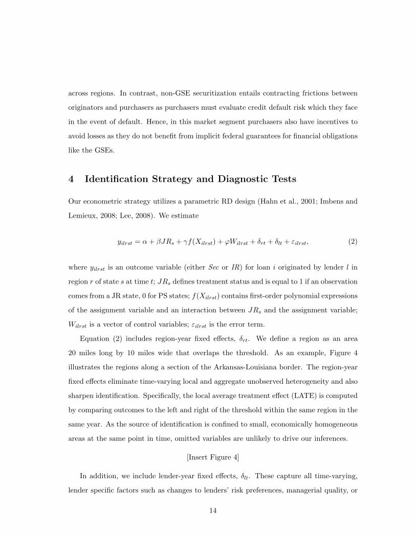
across regions. In contrast, non-GSE securitization entails contracting frictions between
originators and purchasers as purchasers must evaluate credit default risk which they face
in the event of default. Hence, in this market segment purchasers also have incentives to
avoid losses as they do not benefit from implicit federal guarantees for financial obligations
like the GSEs.
4 Identification Strategy and Diagnostic Tests
Our econometric strategy utilizes a parametric RD design (Hahn et al., 2001; Imbens and
Lemieux, 2008; Lee, 2008). We estimate
yilrst = α+ βJRs + γf(Xilrst) + ϕWilrst + δrt + δlt + εilrst, (2)
where yilrst is an outcome variable (either Sec or IR) for loan i originated by lender l in
region r of state s at time t; JRs defines treatment status and is equal to 1 if an observation
comes from a JR state, 0 for PS states; f(Xilrst) contains first-order polynomial expressions
of the assignment variable and an interaction between JRs and the assignment variable;
Wilrst is a vector of control variables; εilrst is the error term.
Equation (2) includes region-year fixed effects, δrt. We define a region as an area
20 miles long by 10 miles wide that overlaps the threshold. As an example, Figure 4
illustrates the regions along a section of the Arkansas-Louisiana border. The region-year
fixed effects eliminate time-varying local and aggregate unobserved heterogeneity and also
sharpen identification. Specifically, the local average treatment effect (LATE) is computed
by comparing outcomes to the left and right of the threshold within the same region in the
same year. As the source of identification is confined to small, economically homogeneous
areas at the same point in time, omitted variables are unlikely to drive our inferences.
[Insert Figure 4]
In addition, we include lender-year fixed effects, δlt. These capture all time-varying,
lender specific factors such as changes to lenders’ risk preferences, managerial quality, or
14

business models that may change over time and impact securitization and pricing decisions.
Lender-year fixed effects also purge time-varying shocks to regulation across different types
of lenders. For example, non-deposit taking institutions are regulated at the state level
whereas domestic banks with national charters and foreign banks are regulated by the
OCC and state chartered banks are supervised by the state regulator in conjunction with
the FDIC or Federal Reserve. Including lender-year fixed effects therefore greatly limits
potential confounds.
4.1 Exogeneity
Critical to our identification strategy is the exogeneity of foreclosure law. Ghent (2014) re-
ports that foreclosure law is exogenous with respect to contemporary economic conditions
and lenders’ behavior because most states’ foreclosure law was determined by idiosyncratic
factors during the pre-Civil War period. For example, the original 13 states inherited JR
law from England. PS law developed during the early eighteenth century in response to
British lenders asking courts to agree to a sale-in-lieu of foreclosure (Ghent, 2014). As the
laws governing foreclosure were determined in case law they have largely endured to the
present day. This is because once there is precedent, the rules a lender must follow rarely
change substantially. Indeed, Ghent (2014) is explicit in her assessment, stating,
“Given the extremely early date at which I find that foreclosure procedures were established,
it is safe to treat differences in some state mortgage laws, at least at present, as exogenous,
which may provide economists with a useful instrument for studying the effect of differences
in creditor rights.”
Other recent papers that treat foreclosure law as exogenous with respect to lender
behavior and contemporary economic matters include Pence (2006), Gerardi et al. (2013),
and Mian et al. (2015).14
14Within the sample there are no changes to state foreclosure laws. Hawaii is the only state that changesthe type of law it uses. See Appendix B for details.
15

4.2 Diagnostic Checks
While treatment status is exogenous in equation (2), the validity of our econometric strat-
egy rests upon two identifying assumptions. First, all other pre-determined factors that
affect securitization must be continuous functions across the threshold. That is, economic
conditions within the treatment and control groups must not systematically differ. If this
assumption is violated, estimates of β will capture both the effect of JR law as well as the
discontinuous factor leading to biased estimates.
Following convention in the literature, Table 3 presents t-tests that inspect whether
the balanced covariates assumption holds in our data. Panel A of Table 3 examines
socioeconomic factors that are common irrespective of loan type between the JR and
PS regions. We find no significant differences in macroeconomic conditions (per capita
income and unemployment), state tax rates, urbanization, the incidence of poverty, ethnic
composition, and educational attainment. Housing markets are strongly similar either side
of the threshold, in terms of house prices, the share of the housing stock that is rented,
and zoning regulations. The rate of renegotiation on delinquent mortgages and the rate
of default on other types of debt are also insignificantly different. The characteristics of
financial intermediaries operating in the regions are highly similar. For example, non-
banks originate an equal share of mortgages in JR and PS regions while banks have
similar capital ratios and Z-scores. There is no significant difference in the share of loans
originated by banks to borrowers outside their headquarter state.
Panel B presents results for a number of variables related to the GSE-eligible loan
sample. We find no significant differences between the treatment and control groups
in terms of applicant income, the gender and ethnic composition of borrowers, borrowers’
FICO scores, and the LTI ratio. While we have somewhat fewer variables available for non-
GSE-eligible loans, Panel C of Table 3 shows no significant differences in the characteristics
of loans either side of the threshold. However, Mian et al. (2015) present evidence that
credit scores, LTV ratios and other homeowner characteristics are continuous across the
JR-PS threshold both in the GSE-eligible and non-GSE-eligible markets. Consistent with
16

Pence (2006), in Panels B and C the only variable that exhibits significant differences is
the loan amount. Lower loan amounts in JR states are consistent with the effects we find
in Section 5.15
[Insert Table 3] [Insert Table 4] [Insert Figure 5]
The second assumption is that neither borrowers nor lenders systematically manip-
ulate treatment status. For example, if risky borrowers strategically decide to purchase
properties in JR states our estimates will be biased due to the composition of borrowers
rather than the impact of foreclosure law. We therefore follow McCrary (2008)’s test for
strategic manipulation by estimating whether the density of mortgage applications and
lender branches per 1,000 population are continuous functions of the threshold. Manipula-
tion by borrowers (lenders) would be consistent with a higher application (lender) density
within JR (PS) states. We estimate the equation
yct = α+ βJRc + γXct + δt + εct, (3)
where yct is either the number of mortgage applications or lenders per 1,000 population
within census tract c time t; JRc is equal to 1 if an observation is from a JR state, 0
otherwise; Xct is a vector of control variables; δt are year fixed effects; εct is the error
term.16
The results of this test are presented in Table 4. We find no evidence of strategic
manipulation by either borrowers or lenders. Specifically, estimates of β are statistically
insignificant throughout columns 1 to 6 of Table 4 irrespective of whether we include
control variables, or estimate equation (3) parametrically or non-parametrically.
Panel A of Figure 5 presents corresponding graphical evidence. The density of loan
applications is continuous across the threshold. Panel B of Figure 5 shows no discontinuity
15The discontinuity in loan amounts does not present an econometric problem because, like securitizationand interest rates, it is not a pre-determined covariate. Rather lower loan amounts are a response to JRlaw.
16We conduct these tests at the census tract level because we require information on the rate of applicationsor the density of lenders.
17
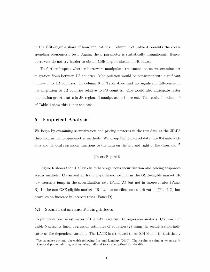
in the GSE-eligible share of loan applications. Column 7 of Table 4 presents the corre-
sponding econometric test. Again, the β parameter is statistically insignificant. Hence,
borrowers do not try harder to obtain GSE-eligible status in JR states.
To further inspect whether borrowers manipulate treatment status we examine net
migration flows between US counties. Manipulation would be consistent with significant
inflows into JR counties. In column 8 of Table 4 we find no significant differences in
net migration to JR counties relative to PS counties. One would also anticipate faster
population growth rates in JR regions if manipulation is present. The results in column 9
of Table 4 show this is not the case.
5 Empirical Analysis
We begin by examining securitization and pricing patterns in the raw data at the JR-PS
threshold using non-parametric methods. We group the loan-level data into 0.4 mile wide
bins and fit local regression functions to the data on the left and right of the threshold.17
[Insert Figure 6]
Figure 6 shows that JR law elicits heterogeneous securitization and pricing responses
across markets. Consistent with our hypotheses, we find in the GSE-eligible market JR
law causes a jump in the securitization rate (Panel A) but not in interest rates (Panel
B). In the non-GSE-eligible market, JR law has no effect on securitization (Panel C) but
provokes an increase in interest rates (Panel D).
5.1 Securitization and Pricing Effects
To pin down precise estimates of the LATE we turn to regression analysis. Column 1 of
Table 5 presents linear regression estimates of equation (2) using the securitization indi-
cator as the dependent variable. The LATE is estimated to be 0.0166 and is statistically
17We calculate optimal bin width following Lee and Lemieux (2010). The results are similar when we fitthe local polynomial regressions using half and twice the optimal bandwidth.
18

significant at the 1% level. Economically, this implies that JR law causes a 4% increase in
the probability that a mortgage loan is securitized, relative to the counterfactual.18 The
evidence is consistent with JR law inducing lenders to transfer foreclosure costs to the
GSEs.
[Insert Table 5]
Among the control variables, we find applicant income and minority status to be
negatively correlated with securitization. The probability of securitization is higher for
loans originated to men and in areas with more lenders per capita. The assignment
variable, and its interaction with the JR indicator, are statistically insignificant. This is
consistent with the relatively flat local regression functions shown in Panel A of Figure
6.19
To ensure our findings are not driven by the limitations of the linear probability model
in the context of a binary dependent variable, we estimate equation (2) using a logit model.
The results of this test in column 2 of Table 5 are very similar to before.20
The effects of JR law on securitization are quite different among non-GSE-eligible
loans. The results in columns 3 and 4 of Table 5 show that JR law has no effect on
securitization in this market. Irrespective of whether we estimate equation (2) using OLS
or a logit model, the JR coefficient is statistically insignificant.
In the remainder of Table 5 we test whether JR law provokes pricing responses across
the different markets. We implement these tests by estimating equation (2) using IR as
the dependent variable. In column 5 of Table 5, we find no discontinuity in interest rates
at the threshold within the GSE-eligible market. However, when we focus on non-GSE-
eligible loans in column 6 of the table, the JR coefficient is equal to 0.0654 and is highly
18To calculate the treatment effect relative to the counterfactual we compare the LATE to the mean rateof securitization within the control group which is 41.5%. Hence, (0.0166/0.415)*100 = 4%.
19Appendix Table A4 shows that JR law has a similar effect on securitization of loans eligible for sale toGinnie Mae.
20The logit estimations include lender, region, and year fixed effects rather than region-year and lender-yearfixed effects. This is because including region-year and lender-year fixed effects results in flat regions inthe maximum likelihood function, preventing identification of the parameters.
19

statistically significant. This is equivalent to increasing interest rates by approximately 7
basis points, or 0.72% relative to the counterfactual.21
To provide further insights into how JR law affects pricing decisions in the non-GSE-
eligible market, we collected information on RMBS deals during our sample period. Each
deal reports the share of the total value of mortgages from JR and PS states. In Appendix
Table A7 we find that RMBS securities’ initial yield is positively and significantly increas-
ing in the share of JR loans within the deal. A one percentage point increase in the JR
share of the deal is associated with a 0.08 percentage point (8 basis points) increase in the
yield. Market participants therefore demand a premium for holding securities that have
greater exposure to JR law and are not protected by GSE guarantees.
The graphical and econometric patterns are consistent with the GSEs’ CIRP and
guarantees inducing securitization to mitigate lenders’ foreclosure losses in the GSE-eligible
market. In the non-GSE-eligible market, where these policies are absent, lenders respond
to JR law by pricing the greater probability of default into mortgage contracts.
Next, we study whether the effects of JR law differ before and after the financial crisis.
Prior to the crisis, house price expectations were high from both a lender and borrower
perspective, securitization of mortgages was common regardless of GSE-eligibility, and
default rates were relatively low. After the crisis, concerns about mortgage default risk
became more prominent, and Fannie Mae and Freddie Mac entered conservatorship which
may influence their purchasing decisions.
[Insert Table 6]
The findings reported in Table 6 for the pre- and post-crisis periods resemble the
21We conduct sensitivity checks to ensure our findings are not due to methodological considerations.Appendix Table A5 reports estimates from models with higher order polynomial expressions of theassignment variable and non-parametric estimates. Table A6 presents results using 5 and 2.5 milebandwidths. In both tables the findings are similar to our baseline estimates. In addition, we estimateequation (2) for each border pair separately to ensure neither outliers nor a limited number of regions drivethe results. Figure A3 shows the positive and statistically significant effect of JR law on securitization(interest rates) in the GSE-eligible (non-GSE-eligible) market is present in the overwhelming majorityof border pairs. Furthermore, the figure shows the insignificant relationship between JR law and interestrates (securitization) in the GSE-eligible (non-GSE-eligible) market for most border pairs.
20

baseline estimates.22 Specifically, we find JR law has a positive and statistically significant
effect on GSE-eligible securitization during both periods. Likewise, JR law causes an
increase in non-GSE-eligible interest rates before and after the crisis. The prevailing effect
of JR law on lenders’ securitization and pricing strategies is consistent with the fact that
default is consistently higher in JR regions across time periods (Demiroglu et al., 2014).
[Insert Table 7]
So far, our econometric strategy has eliminated omitted variables by including region-
year and lender-year fixed effects in the estimating equations. To rule out time-varying
local shocks, we exploit the panel structure of the data using difference-in-difference esti-
mation. Specifically, we evaluate whether JR law differentially affects the probability of
securitization or interest rates on GSE-eligible relative to non-GSE-eligible loans within
an area at a given point in time. We estimate the equation
yilrst = αGSEilrst + βJRs ∗GSEilrst + ϕWilrst + δlt + δct + εilrst, (4)
where GSEilrst is a dummy variable equal to 1 if a loan is GSE-eligible, 0 for non-GSE-
eligible loans; δct are census tract-year fixed effects; all other variables are defined as
previously. In view of our previous results, one would expect estimates of β to be positive
in the securitization tests (JR law increases the probability that GSE-eligible loans are
securitized relative to non-GSE-eligible loans) and negative in the interest rate tests (JR
law increases the interest rate of non-GSE-eligible loans relative to GSE-eligible loans).
Column 1 of Table 7 provides estimates of equation (4) using the securitization indica-
tor as the dependent variable. The GSE coefficient is positive and statistically significant,
consistent with lenders securitizing GSE-eligible loans more frequently compared to non-
GSE-eligible loans, regardless of JR law. The JR-GSE interaction coefficient is positive
and highly statistically significant. Hence, at a given point in time within a census tract,
22We define the pre-crisis period as the years 2000 to 2006 and the post-crisis period as the years 2010 to2016.
21

JR law induces lenders to securitize GSE-eligible loans at a significantly higher probability
relative to non-GSE-eligible loans.
Column 2 of the table presents the results for interest rates. The GSE coefficient is
negative, indicating that interest rates charged on GSE-eligible loans are lower compared
to non-GSE-eligible interest rates. In addition, the interaction coefficient is negative and
statistically significant at the 1% level, implying that within an area at a given point in
time, JR law increases the interest rate on non-GSE-eligible loans by approximately 0.3
percentage points relative to rates on GSE-eligible loans. Together these findings rule out
that time-varying local conditions drive our previous inferences.
5.2 Expected Costs of Default Mechanism
Underpinning our tests is the hypothesis that JR law increases lenders’ cost of default. We
therefore conduct a series of sub-sample tests to validate this mechanism. Intuitively, the
effects of JR law should be more pronounced within samples comprising riskier borrowers
where JR law has the largest effect on the incentive to default.
[Insert Table 8]
Panel A of Table 8 reports estimates of equation (2) for GSE-eligible securitization.
One would anticipate relatively larger LATEs among low- versus high-income borrowers.
The probability of default is increasing in the LTI ratio as borrowers are more susceptible
to shocks that compromise their ability to meet mortgage payments. Similarly, loans to
borrowers with co-applicants are potentially less prone to default because multiple income
streams help smooth negative economic shocks. Consistent with these conjectures, the
estimates in columns 1 to 6 of Table 8 show the LATE is larger for loans with income
below relative to above the mean, for high relative to low LTI loans, and for loans to sole
relative to co-applicants.
In the remainder of Panel A, we split the sample based on socioeconomic conditions
in the area where the borrower’s house is located. In columns 7 and 8 we find that
22

the probability of securitization in response to JR law is substantially larger for loans
originated to borrowers who live in high relative to low unemployment areas. We obtain
similar results in columns 9 and 10 of the table when we split the sample based on the
poverty rate.
Panel B and Panel C of Table 8 repeat the subsample tests for GSE-eligible inter-
est rates and non-GSE-eligible securitization, respectively. Consistent with our previous
results, the LATE is statistically insignificant throughout both panels.
Finally, we report estimates of subsample tests for non-GSE-eligible interest rates in
Panel D of Table 8. A consistent pattern emerges. As before, JR law causes a significant
increase in interest rates among non-GSE-eligible loans. However, the magnitude of this
response is considerably larger in the categories where expected default costs are higher.
For example, for borrowers with below mean income, JR law increases interest rates by
approximately 0.08 percentage points versus 0.02 percentage points for applicants with
income greater than or equal to average income. The JR coefficient is somewhat smaller
for loans where the LTI ratio is below the mean compared loans with an LTI ratio greater
than or equal to the mean. The coapplicant, unemployment, and poverty rate sample
splits provide similar inferences.23
5.3 Which Channel Matters Most?
So far, the empirical findings demonstrate that JR law provokes heterogeneous securiti-
zation and pricing reactions across market segments. Our next set of tests establish the
source of this effect. Does JR law matter because it raises lenders’ legal costs or because
it increases borrowers’ default incentives? Resolving these questions is essential for the
design of policy.
23Our last test follows the approach used by Agarwal et al. (2012) to calculate the predicted probabilityof default for each loan. We then split the sample according to whether the probability of default liesabove or below the mean. The results in Appendix Table A8 show that the JR coefficient is positive andstatistically significant in both subsamples for GSE-eligible securitization and non-GSE-eligible interestrates. However, in both cases, the effect of JR law is more pronounced for loans with default probabilitiesabove the mean.
23

[Insert Table 9]
The identifying assumption in these tests is that legal costs and foreclosure timelines
vary exogenously. This seems plausible as both variables are functions of exogenous fore-
closure law. To enable comparability of economic magnitudes we use standardized legal
cost and timeline variables. Column 1 in Table 9 shows a standard deviation increase
in lenders’ legal costs of foreclosure leads to a statistically significant 0.79% increase in
the probability that a GSE-eligible loan is securitized. However, GSE-eligible securitiza-
tion is more responsive to increasing the foreclosure timeline. The standardized timeline
coefficient is equivalent to a 1.94% increase in the probability of securitization. In the
non-GSE-eligible market, we also find foreclosure timelines have a relatively larger im-
pact on interest rates. In column 2 of the table the standardized legal cost and timeline
coefficients are 0.0544 and 0.0978, respectively.
Hence, while both channels matter, the effect of JR law on GSE-eligible securitization
and non-GSE-eligible interest rates is primarily transmitted through raising borrowers’
default incentives. This implies that initiatives that speed up court procedures and shorten
the foreclosure process may mitigate the distorting effects of JR law by reducing moral
hazard among borrowers and lowering lenders’ expected losses.
5.4 Alternative Explanations: Borrower Quality
A natural question is whether the effect of JR law on securitization and interest rates is
due to differences in borrowers’ characteristics either side of the threshold. We therefore
conduct sensitivity checks to inspect this channel.
[Insert Table 10]
Table 10 presents estimates of equation (2) with borrower credit quality controls. In
column 1 of the table, we report results for GSE-securitization that include the LTI ratio,
term to maturity, FICO scores, the DTI ratio, and mortgage insurance as further controls.
We continue to find the JR coefficient is positive and statistically significant. In column
24

2 we report the corresponding results for GSE-eligible interest rates. As before, the JR
coefficient remains statistically insignificant. Columns 3 and 4 provide results for the same
tests in the non-GSE-eligible market. Data constraints mean we are limited to measuring
creditworthiness using the LTI ratio and term to maturity variables. Nevertheless, the
pattern of results is the same as in the baseline specifications. Despite controlling for
these factors, JR law has no significant effect on securitization of non-GSE-eligible loans,
but leads to a significant increase in interest rates.
6 Robustness Checks
In this section, we conduct robustness tests to ensure omitted variables to not contaminate
the results.
6.1 Placebo Tests
A concern is that the relationship between the outcome variables and foreclosure law
is discontinuous at the threshold due to jumps in other factors. Placebo tests provide
inferences into whether JR law drives the behavior we observe in the data. Specifically, in
samples where foreclosure law is continuous across the threshold, we should not observe
discontinuities in securitization or interest rates. We therefore estimate the equation
yilrst = βP lacebos + γf(Dilrst) + ϕWilrst + δrt + δlt + εilrst, (5)
where all variables are the same as in equation (2) except Placebos which is a dummy
variable equal to 1 on the right of the placebo threshold, 0 on the left of the placebo
threshold; and Dilrst contains the distance to the placebo threshold and an interaction
between the placebo assignment variable and Placebos.
We first estimate equation (5) using observations within 10 miles of a placebo threshold
located 10 miles to the right of the actual threshold where JR law governs the foreclosure
process on both sides. The results reported in Panel A of Table 11 show the placebo
25

coefficient is statistically insignificant throughout all specifications. Neither the likelihood
of securitization nor interest rates in the GSE and non-GSE markets are discontinuous at
the placebo threshold. Next, we repeat the procedure using observations within 10 miles
of a placebo threshold 10 miles to the left of the actual threshold, where PS law regulates
the foreclosure process either side. In Panel B of Table 11 the placebo LATEs are again
statistically insignificant.
[Insert Table 11]
To affirm our baseline estimates do not simply capture border effects, other aspects of
the legal environment, or political economy considerations, we use samples drawn around
the border between states that use the same foreclosure law. We randomly assign states to
placebo treatment and placebo control status and estimate equation (5). Panel C (D) of
Table 11 provides results from JR-JR (PS-PS) borders. The placebo coefficient estimate
is again statistically insignificant. Appendix Figures A4 and A5 report placebo estimates
for each individual border pair along JR-JR and PS-PS borders, respectively. The placebo
coefficient estimate is insignificant in almost all instances.
If an omitted variable drives our main findings, the placebo LATEs should be similar in
magnitude and statistical significance as the baseline estimates. Throughout Table 11 this
is not the case. That securitization and interest rates only jump at the actual threshold
where there exist discontinuities in the laws governing foreclosure reinforces our argument
that the effects we observe are not driven by observable or unobservable omitted variables.
6.2 The Legal Environment
The next set of tests focus on whether other aspects of the state-level legal environment
confound our inferences. For example, right of redemption (ROR) law allows borrowers to
redeem their property within 12 months of foreclosure, potentially imposing further costs
on lenders. Lenders may pursue delinquent borrowers’ future income to cover unpaid
foreclosure debts using deficiency judgments. Prior research has also documented a link
26

between mortgage default and bankruptcy exemptions (Lin, 2001).24 We therefore append
equation (2) with controls for these factors and test the sensitivity of our results. In
columns 1 to 3 of Panels A to D in Table 12 the JR coefficient remains similar to before.
[Insert Table 12]
Recent evidence suggests deregulation of mortgage brokering reduced screening of loan
applications leading to riskier lending (Shi and Zhang, 2018). As mortgage brokers are
not exposed to the cost of default but their profits are increasing in the number of loan
applications they process, lifting restrictions on broker services may create moral hazard
and expose lenders to riskier borrowers. We therefore add the state-level broker restric-
tiveness index as a further control to the estimating equation and report the estimates in
column 4 of Table 12. The key findings remain intact.
The Bankruptcy Abuse Prevention and Consumer Protection Act of 2005 (BAPCPA)
made it more difficult for individuals to declare bankruptcy. This potentially reduced the
incentive to default upon mortgage payments. It seems implausible that the BAPCPA
drives our inferences as it is a federal law that applies across the threshold and is captured
by the region-year fixed effects. However, we report estimates using a sample that excludes
the years 2005 to 2016 in column 6 of Table 12. The effect of JR law on securitization is
very similar to before.
The Dodd-Frank Act of 2010 implemented a number of changes that strengthened
regulation of financial intermediaries. This was also a federal law that applies to both
sides of the threshold. Nevertheless, the results in column 7 of Table 12 demonstrate that
excluding observations from the years 2010 to 2016 from the sample has no bearing on
our inferences.
Appendix Table A9 presents further legal robustness tests. We test the sensitivity of
24Homestead exemptions are the most important bankruptcy exemption and evidence shows that mortgagedefault is more likely the more generous are homestead exemptions (Lin, 2001). Nonhomestead exemp-tions allow individuals to maintain wealth in other asset categories but tend to be set at low levels.For example, the mean homestead exemption across US states is $122,754 whereas the mean nonhome-stead exemption (comprising automobile, other property (clothing, jewelry, and tools), and wildcardexemptions) is $19,685.
27

our findings to 1) excluding observations from Delaware and Pennsylvania which use scire
facias, a creditor-friendly form of JR law,25 2) excluding Texas as it is the only state that
limits the LTV ratio of mortgages to 80%, 3) excluding Louisiana from the sample on
the grounds that it is the only Civil Law state, and 4) excluding Massachusetts which
undertakes reforms to speed up foreclosure timelines during the sample period (Gerardi
et al., 2013). Throughout Panels A and B of Table A9, the JR law coefficient remains
robust despite these changes.
6.3 Lending Industry Conditions
Approximately half the loans in our sample are originated by deposit-taking institutions
(banks) with the remainder supplied by non-depository institutions (non-banks). Non-
banks typically rely on short-term wholesale market funding and are thus more likely to
securitize loans to ensure repayment. To avoid that our findings reflect a higher concentra-
tion of different lender types either side of the threshold, we split the sample and estimate
equation (2) using non-banks and banks separately. The results in columns 1 and 2 of
Table 13 show that JR law has a positive and highly statistically significant effect on the
probability that a loan is securitized within both sub-samples.
[Insert Table 13]
Next, we examine the sensitivity of our findings to conditions within the banking
industry. First, we append equation (2) with bank-level covariates to capture bank size,
profitability, soundness, and capitalization.26 The JR coefficient estimate in column 3 of
Table 13 is invariant to this change. In column 4 of the table, we report results that
include the cost of deposits as a further control variable. Our findings remain robust.
25Scire facias places the onus on the borrower to provide a reason why the lender should not be able toforeclose (Ghent, 2014). Despite its perceived creditor-friendly nature, scire facias is neither expedientnor cheap for lenders. Data from the SFLD show the foreclosure timeline is longer and average foreclosurecost to lenders is higher in Delaware and Pennsylvania relative to other JR states (see Table A2).
26To implement this test we must include lender fixed effects rather than lender-year fixed effects in theestimating equation.
28

For banks, cross-border lending is permitted. If a state regulator is more lenient on
out-of-state activities compared to lending at home (Ongena et al., 2013), this may pose
a problem if the PS state is more often the home state and the regulator dislikes the OTD
model at home. The estimates in column 5 of Table 13 allay these concerns.
Banks are subject to different regulators depending on their charter. To ensure reg-
ulatory differences do not confound our results, we split the sample and focus on state
chartered and national chartered banks separately. Columns 6 and 7 of Table 13 report the
estimates for the sample using state chartered and national chartered banks, respectively.
The JR law coefficient is positive and statistically significant in both columns.
Geographic diversification may affect banks’ ability to attract deposit funds, thereby
influencing their securitization decisions. We therefore constrain the sample to loans orig-
inated by banks that operate in only one state and report the estimates in column 8 of
Table 13. Our key finding is preserved. Similarly, when we focus exclusively on loans
originated by multi-state banks in column 9, our inferences endure.
Next, we check whether the nature of banks’ business models drives our results. A
concern is that banks operating OTD models are highly dependent on selling loans. If such
institutions are disproportionately clustered on the JR side of the threshold, our estimates
will conflate banks’ business models with the effect of JR law. To address this concern
we focus exclusively on banks that do not operate an OTD model, defined as banks that
securitize less than 50% of the mortgage loans they originate. The results in column 10 of
Table 13 are very similar to before.
6.4 Miscellaneous Sensitivity Checks
We conduct a number of robustness tests to ensure our findings do not reflect differences
in zoning restrictions between states, the general riskiness of the population that live
in border areas measured using delinquency rates on auto and credit card loans, and
competition between lenders. In addition, we inspect whether the longer timeline in JR
states allows delinquent borrowers to self-cure and renegotiate terms with the mortgage
29

servicer. Meanwhile lenders’ profitability expectations are influenced by pre-payment risk,
and changes in interest rates on adjustable rate loans. Han et al. (2015) report evidence
that tax rates can motivate securitization. The findings reported in Tables A10 and A11
demonstrate none of these factors confound our inferences.
Finally, in Table A12 we sequentially focus on specific US regions. Panel A (B) of the
table reports estimates using observations from the most (least) populous border regions.
As before, we find JR law causes a significant increase in GSE-eligible securitization and
non-GSE-eligible interest rates regardless of population. In Panels C to G of Table A12 we
focus on samples drawn from within the Northeast, Midwest, West, and Southern states.
Our findings remain remarkably stable.
7 Conclusions
We show that, in markets where JR law governs the foreclosure process, lenders exhibit an
excessive propensity to securitize GSE-eligible mortgage loans. Baseline estimates show
JR law causes a 4% increase in the probability of securitization. The magnitude of the JR
effect size is considerably larger among samples of borrowers where default is more likely
to occur. In contrast, JR law has no effect on securitization among non-GSE-eligible loans
but instead provokes a 7 basis point increase in interest rates.
These findings have important policy implications. During the US Foreclosure Crisis
of 2010, 4 million homes were improperly foreclosed. Recent policy initiatives seek to
address this issue by extending greater protections to borrowers. An important insight of
our research is the trade-offs this involves. Protecting borrowers’ rights leads to higher
expected costs of default for lenders, but these costs are largely borne by taxpayers.
Our work has broader implications for the debate on reforming the GSEs. The effects
of the CIRP have yet to receive attention. Owing to the CIRP, lenders do not price
the systematically higher rates of default in JR regions into mortgage contracts. Instead
lenders strategically unload approximately $80 billion of GSE-eligible mortgage debt from
JR states onto the GSEs each year. This increases taxpayers’ exposure to mortgage
30

markets, and may impose greater losses during housing market downturns.
Tackling these issues may involve reforming the GSEs’ CIRP, purchase guarantees, and
introducing private capitalization. However, our evidence demonstrates that addressing
elements of the legal environment also warrant attention. As JR law primarily affects secu-
ritization and pricing behavior by increasing the foreclosure timeline, policy interventions
aiming to improve the speed of judicial procedures may help limit the extent to which
lenders exploit the GSEs’ guarantees to circumvent the CIRP.
The mechanism highlighted in this paper has bearings beyond the context of the hous-
ing market. In particular, it has implications for risk transfer behavior in any secondary
market. There may also be other laws and housing market frictions that have a more
distortionary impact than JR law. Exploring other areas in which lenders share default
losses with third parties is an exciting avenue for future research.
References
Agarwal, S., Amromin, G., Ben-David, C., Chomsisengphet, S., and Evanoff, D. (2011).
The role of securitization in mortgage renegotiation. Journal of Financial Economics,
102(3):559–578.
Agarwal, S., Chang, Y., and Yavas, A. (2012). Adverse selection in mortgage securitization.
Journal of Financial Economics, 105(3):640–660.
Bayer, P., Ferreira, F., and Ross, S. (2018). What drives racial and ethnic differences
in high-cost mortgages? The role of high-risk lenders. Review of Financial Studies,
31(1):175–205.
Calder, V. (2017). Zoning, land-use planning, and housing affordability. Cato Institute
Policy Analysis No. 823.
Clauretie, T. and Herzog, T. (1990). The effect of state foreclosure laws on loan losses:
31

Evidence from the mortgage industry. Journal of Money, Credit and Banking, 22(2):221–
233.
Corradin, S., Gropp, R., Huizinga, H., and Laeven, L. (2016). The effect of personal
bankruptcy exemptions on investment in home equity. Journal of Financial Intermedi-
ation, 25:77–98.
Dahger, J. and Sun, Y. (2016). Borrower protection and the supply of credit: Evidence
from foreclosure laws. Journal of Financial Economics, 121(1):195–209.
Demiroglu, C., Dudley, E., and James, C. M. (2014). State foreclosure laws and the
incidence of mortgage default. Journal of Law and Economics, 57(1):225–280.
Diamond, D. (1984). Financial intermediation and delegated monitoring. Review of Eco-
nomic Studies, 51(3):393–414.
Diamond, D. and Rajan, R. (2006). Money in a theory of banking. American Economic
Review, 96(1):30–53.
Elenev, V., Landvoigt, T., and Van Nieuwerburgh, S. (2016). Phasing out the GSEs.
Journal of Monetary Economics, 81(C):111–132.
Frame, W. S. and White, L. J. (2005). Fussing and fuming over Fannie and Freddie: How
much smoke, how much fire? Journal of Economic Perspectives, 19(2):159–184.
Gerardi, K., Lambie-Hanson, L., and Willen, P. (2013). Do borrower rights improve bor-
rower outcomes? Evidence from the foreclosure process. Journal of Urban Economics,
73(1):1–17.
Gete, P. and Zecchetto, F. (2018). Distributional implications of government guarantees
in mortgage markets. Review of Financial Studies, 31(3):1064–1097.
Ghent, A. (2014). How do case law and statute differ? Lessons from the evolution of
mortgage law. Journal of Law and Economics, 57(4):1085–1122.
32

Ghent, A. C. and Kudlyak, M. (2011). Recourse and residential mortgage default: Evi-
dence from US states. Review of Financial Studies, 124(9):3139–3186.
Glaeser, E. and Gyourko, J. (2002). The impact of zoning on housing affordability. NBER
Working Paper No. 8835.
Gorton, G. and Pennacchi, G. (1995). Banks and loan sales marketing nonmarketable
assets. Journal of Monetary Economics, 35(3):389–411.
Hahn, J., Todd, P., and Van der Klaauw, W. (2001). Identification and estimation of
treatment effects with a regression discontinuity design. Econometrica, 69(1):201–209.
Han, J., Park, K., and Pennacchi, G. (2015). Corporate taxes and securitization. Journal
of Finance, 70(3):1287–1321.
Holmstrom, B. and Tirole, J. (1997). Financial intermediation, loanable funds, and the
real sector. Quarterly Journal of Economics, 112(3):663–691.
Imbens, G. W. and Lemieux, T. (2008). Regression discontinuity designs: A guide to
practice. Journal of Econometrics, 142(2):615–635.
Jeske, K., Krueger, D., and Mitman, K. (2013). Housing, mortgage bailout guarantees
and the macro economy. Journal of Monetary Economics, 60(8):917–935.
Keys, B., Mukherjee, T., Seru, A., and Vig, V. (2010). Did securitization lead to lax
screening? Evidence from subprime loans. Quarterly Journal of Economics, 125(1):307–
362.
Keys, B., Seru, A., and Vig, V. (2012). Lender screening and the role of securitization:
Evidence from prime and subprime mortgage markets. Review of Financial Studies,
25(7):2071–2108.
Lee, D. (2008). Randomized experiments from non-random selection in U.S. house elec-
tions. Journal of Econometrics, 142(2):675–697.
33

Lee, D. S. and Lemieux, T. (2010). Regression discontinuity designs in economics. Journal
of Economic Literature, 48(2):281–355.
Lin, E.Y. White, M. (2001). Bankruptcy and the market for mortgage and home improve-
ment loans. Journal of Urban Economics, 50(1):138–162.
McCrary, J. (2008). Manipulation of the running variable in the regression discontinuity
design: A density test. Journal of Econometrics, 142(2):698–714.
Melzer, B. T. (2017). Mortgage debt overhang: Reduced investment by homeowners at
risk of default. Journal of Finance, 72(2):575–612.
Mian, A., Sufi, A., and Trebbi, F. (2015). Foreclosures, house prices, and the real economy.
Journal of Finance, 70(6):2587–2634.
Ongena, S., Popov, A., and Udell, G. (2013). When the cat’s away the mice will play: Does
regulation at home affect bank risk-taking abroad? Journal of Financial Economics,
108(3):727–750.
Pahl, C. (2007). A compilation of state mortgage broker laws and regulations, 1996-2006.
Federal Reserve Bank of Minneapolis, Community Affairs Report, No. 2007-2.
Pence, K. M. (2006). Foreclosing on opportunity: State laws and mortgage credit. Review
of Economics and Statistics, 88(1):177–182.
Piskorski, T., Seru, A., and Vig, V. (2010). Securitization and distressed loan renegoti-
ation: Evidence from the subprime mortgage crisis. Journal of Financial Economics,
97(3):369–397.
Purnanandam, A. (2010). Originate-to-distribute model and the subprime mortgage crisis.
Review of Financial Studies, 24(6):1881–1915.
Schill, M. (1991). An economic analysis of mortgagor protection laws. Virginia Law
Review, 77(3):489–538.
34

Seiler, M., Seiler, V., Lane, M., and Harrison, D. (2012). Fear, shame and guilt: Economic
and behavioral motivations for strategic default. Real Estate Economics, 40(1):199–233.
Shi, L. and Zhang, Y. (2018). The effect of mortgage broker licensing under the originate-
to-distribute model: Evidence from the U.S. mortgage market. Journal of Financial
Intermediation, 35(A):70–85.
35

Tab
les
Tab
le1:
Su
mm
ary
Sta
tist
ics
Var
iable
Mea
nStd
.D
ev.
Min
Max
Obse
rvat
ions
Sou
rce
Sec
(GSE
-eligi
ble
)0.
4252
0.48
850
148
5,26
7H
MD
ASec
(Non
-GSE
-eligi
ble
)0.
4734
0.49
910
174
,799
HM
DA
IR(G
SE
-eligi
ble
)6.
753
0.53
975.
7453
8.35
0947
5,99
8SF
LD
IR(N
on-G
SE
-eligi
ble
)10
.710
21.
4698
8.24
6612
.435
568
,978
HM
DA
JR
(Dum
my)
0.39
740.
4894
01
560,
066
App
endix
BA
ssig
nm
ent
(Miles
)-0
.647
75.
0746
-9.9
994
9.99
9956
0,06
6A
uth
ors’
calc
ula
tion
sG
SE
-eligi
ble
(Dum
my)
0.86
650.
3401
01
560,
066
HM
DA
Loa
nam
ount
(Ln)
4.73
670.
8610
1.38
6211
.289
756
0,06
6H
MD
AA
pplica
nt
inco
me
(Ln)
11.1
670.
6291
9.68
0312
.624
856
0,06
6H
MD
AM
ale
(Dum
my)
0.66
140.
4732
01
560,
066
HM
DA
Min
orit
y(D
um
my)
0.21
390.
4101
01
560,
066
HM
DA
Coa
pplica
nt
(Dum
my)
0.62
770.
4834
01
560,
066
HM
DA
LT
Ira
tio
1.99
111.
1311
0.08
114.
9333
560,
066
HM
DA
Len
der
sp
erca
pit
a0.
6400
0.58
000.
1170
3.03
4156
0,06
6A
uth
ors
’ca
lcula
tion
sA
pplica
tion
sp
erca
pit
a15
.603
420
.164
20.
7082
78.7
671
560,
066
Auth
ors
’ca
lcula
tion
sH
ouse
pri
cein
dex
12.5
505
0.92
769.
5384
14.6
628
560,
066
FH
FA
Ren
ter
occ
upie
dhou
sing
(%)
26.6
368
16.7
623
2.3
81.6
560,
066
US
Cen
sus
Arr
ange
men
tfe
e(%
)0.
7169
0.35
540.
011.
5456
0,06
6F
HFA
Ter
mto
mat
uri
ty(y
ears
)29
.893
40.
9523
24.1
200
31.4
700
560,
066
FH
FA
Mor
tgag
ein
sura
nce
(%)
23.9
767
0.76
6720
.25
27.2
502
475,
998
SF
LD
DT
Ira
tio
(%)
34.7
236
2.40
5528
.960
139
.964
747
5,99
8SF
LD
Ori
ginal
LT
V(%
)76
.5053
2.86
7567
.915
381
.015
647
5,99
8SF
LD
FIC
O71
8.89
196.
8845
682.
4072
734.
7451
560,
066
SF
LD
Rig
ht
ofre
dem
pti
on(D
um
my)
0.63
23
0.48
220
156
0,06
6G
hen
tan
dK
udly
ak(2
011)
36

Tab
le1
Con
t’d
:S
um
mar
yS
tati
stic
s
Var
iable
Mea
nStd
.D
ev.
Min
Max
Obse
rvat
ions
Sourc
e
Defi
cien
cyju
dge
men
t(D
um
my)
0.96
670.
1793
01
560,
066
Ghen
tand
Kudly
ak
(2011
)B
roke
rre
stri
ctiv
enes
sin
dex
6.18
754.
0312
016
560,
066
Pah
l(2
007)
Hom
este
adex
empti
on(L
n)
10.1
075
1.03
394.
1352
13.1
224
560,
066
Cor
radin
etal.
(201
6)
Non
hom
este
adex
empti
on(L
n)
8.70
250.
7673
5.70
3811
.245
056
0,06
6C
orr
adin
etal
.(2
016)
Zon
ing
index
25.6
675
13.6
288
150
560,
066
Cald
er(2
017
)L
egal
cost
(USD
thou
sands)
4.50
171.
9362
2.21
4914
.810
056
0,06
6SF
LD
Tim
elin
e(D
ays)
110.
3006
78.3
560
2744
556
0,06
6U
SF
NR
eneg
otia
tion
rate
(%)
0.05
340.
2018
02.
501
475,
998
SF
LD
Refi
nan
cing
rate
(%)
50.9
244
12.0
926
24.3
455
75.5
9799
560,
066
HM
DA
Sta
teco
rpor
ate
tax
rate
(%)
6.92
021.
6546
09.
9956
0,06
6T
ax
Fou
ndat
ion
Sta
tep
erso
nal
tax
rate
(%)
5.35
252.
3695
012
560,
066
Tax
Fou
ndat
ion
Auto
del
inquen
cyra
te(%
)3.
3827
2.07
790
26.2
356
0,06
6N
YF
edC
redit
card
del
inquen
cyra
te(%
)9.
9756
3.50
143.
6320
.740
156
0,06
6N
YF
edA
dju
stab
lera
telo
ans
(%)
15.8
673
9.59
980
5556
0,06
6F
HFA
HH
I(L
n)
10.2
547
1.30
896.
3946
14.0
805
560,
066
Auth
or’
sca
lcula
tion
Ban
ksi
ze(L
n)
16.8
642
3.01
1311
.25
21.0
524
277,
545
FD
ICZ
-sco
re(L
n)
3.25
690.
9331
1.39
365.
7956
277,
545
FD
ICC
apit
alra
tio
(%)
10.4
942
5.21
631.
0016
16.1
681
277,
545
FD
ICN
on-b
ank
(Dum
my)
0.50
440.
4984
01
560,
066
Auth
ors’
calc
ula
tion
sN
IIra
tio
(%)
3.32
770.
7538
1.43
277.
5768
277,
545
FD
ICC
ost
ofdep
osit
s(%
)1.
6333
4.90
020.
0010
18.7
343
277,
545
FD
ICO
ut
ofst
ate
(Dum
my)
0.11
230.
3157
01
560,
066
HM
DA
Unem
plo
ym
ent
rate
(%)
5.00
551.
0743
1.6
11.8
560,
066
BE
AP
erca
pit
ain
com
e(L
n)
10.3
768
0.24
689.
819
10.9
310
560,
066
BE
AU
rban
izat
ion
(Dum
my)
0.88
660.
3171
01
560,
066
US
Cen
sus
Pov
erty
rate
(%)
11.5
062
3.93
462.
641
.956
0,06
6U
SC
ensu
sB
lack
pop
ula
tion
(%)
10.3
354
8.02
100.
0246
63.5
077
560,
066
US
Cen
sus
His
pan
icp
opula
tion
(%)
4.37
094.
6733
0.29
1182
.205
156
0,06
6U
SC
ensu
sV
iole
nt
crim
era
te(%
)0.
0040
0.00
180
0.02
5256
0,06
6U
SC
ensu
sD
egre
e(%
)25
.100
67.
5011
8.45
0063
.756
0,06
6U
SC
ensu
sN
etm
igra
tion
(%)
-0.0
113
2.31
67-0
.111
50.
6129
430,
832
Auth
ors’
calc
ula
tion
sP
opula
tion
(%)
0.71
002.
1641
-4.0
577
7.48
9649
,783
Auth
ors’
calc
ula
tion
s
Note
s:T
his
table
pro
vid
esdes
crip
tive
stati
stic
sfo
rth
eva
riable
suse
din
the
empir
ical
analy
sis.
Fore
closu
reco
stis
mea
sure
din
thousa
nds
of
US$
(defl
ate
din
to2016
pri
ces)
.L
ender
sp
erca
pit
aand
Applica
tions
per
capit
aare
mea
sure
dp
er1,0
00
popula
tion.
’Ln’
den
ote
sth
at
ava
riable
ism
easu
red
innatu
ral
logari
thm
s.’S
ourc
e’den
ote
sth
edata
pro
vid
er.
BE
Aden
ote
sth
eB
ure
au
of
Eco
nom
icA
naly
sis.
FH
FA
den
ote
sth
eF
eder
al
Housi
ng
Fin
ance
Agen
cy.
FD
ICden
ote
sth
eF
eder
al
Dep
osi
tIn
sura
nce
Corp
ora
tion.
USF
Nden
ote
sth
eU
SF
ore
closu
reN
etw
ork
.
37

Table 2: Probability of Default and Foreclosure Costs
1 2 3 4Dependent variable Cost Cost Default Default
JR 0.5033*** 0.5223*** 0.0021*** 0.0028***(14.85) (13.54) (15.91) (21.87)
Per capita income 0.0031 -0.0065***(0.04) (-44.68)
DTI ratio 0.0187 0.0014***(0.86) (10.79)
Term to maturity -0.0127 0.0002***(-0.76) (8.63)
House price index 0.3258** 0.0113***(2.42) (43.79)
Lender FE Yes Yes Yes YesYear FE Yes Yes Yes Yes
Observations 17,091 17,091 2,182,591 2,182,591R2 0.05 0.05 0.09 0.10
Notes: This table presents estimates of equation (1). Cost includes legal costs, associated taxes, propertymaintenance cost after foreclosing and miscellaneous costs (in natural logarithms). The sample in columns1 and 2 use only observations where default has occurred. Standard errors are clustered at the state leveland the corresponding t-statistics are reported in parentheses. ** and *** indicate statistical significanceat the 5% and 1% levels, respectively.
38

Table 3: Balanced Covariates Tests
Variable JR PS Difference t-statistic
Panel A: Socioeconomic conditions
Per capita income 10.3246 10.4287 -0.1041 -1.37Unemployment rate 4.9108 4.9240 -0.0132 -0.04State corporate tax rate 6.4256 6.4446 -0.0190 -0.54State personal tax rate 5.0226 5.0472 -0.0246 -0.80Urbanization 0.8547 0.8619 -0.0072 -0.33Poverty rate 11.42 11.45 -0.03 -0.15Black population 11.28 11.17 0.11 0.14Hispanic population 4.40 4.57 -0.17 -0.54Degree 24.8551 24.8495 0.0056 0.55House price index 12.3201 12.4133 -0.0932 -1.07Refinancing rate 50.1657 51.4247 -1.2589 -1.01Renter occupied housing 25.8943 25.8011 0.0933 0.90Renegotiation rate 0.0545 0.0557 -0.0012 -0.11Auto delinquency rate 3.4688 3.4984 -0.0296 -0.15Credit card delinquency rate 4.5104 4.4894 0.0210 0.89Violent crime rate 0.0015 0.0016 -0.0001 -0.15HHI 9.9927 10.0652 -0.0725 1.07Lenders per capita 0.6840 0.6881 -0.0040 -0.10Non-bank 0.5056 0.5005 0.0051 0.33Z-score 3.6501 3.6102 0.0399 1.02Capital ratio 10.5613 10.4860 0.0753 0.15Out of state loan 0.1115 0.1127 -0.0012 -1.41
Panel B: GSE-eligible loans
Applicant income 11.0433 11.0638 -0.0205 -1.30Loan amount 4.6963 4.7135 -0.0172** -2.33Male 0.5915 0.55831 0.0084 1.51Minority 0.1194 0.1176 0.0018 0.50LTI ratio 1.9331 1.9412 -0.0081 -0.50Term to maturity 29.9167 29.8982 0.0185 1.36Mortgage insurance 24.0409 24.0465 -0.0056 -0.32DTI ratio 34.6704 34.6676 0.0028 0.02Original LTV 76.6345 76.7846 -0.1501 -0.81FICO 717.2855 716.9007 0.3848 1.55Arrangement fee 1.2749 1.2990 -0.0241 -0.71
Panel C: Non-GSE-eligible loans
Applicant income 11.0779 11.1047 -0.0268 -1.41Loan amount 4.4342 4.4864 -0.0522** -2.49Male applicant 0.5939 0.5862 0.0077 1.55Minority applicant 0.1207 0.1176 0.0031 0.72LTI ratio 1.9246 1.9313 -0.0067 0.87
Notes: This table reports the results of t-tests for differences in the average level of each covariate betweenthe JR and PS regions either side of the threshold. JR and PS denote the mean of each variable on theJR and PS side of the threshold, respectively. Difference is the difference between JR and PS. The nullhypothesis is that JR = PS. t-statistic is the t-statistic from a two-tailed test of the null hypothesis thatDifference is equal to zero. Panel A reports estimates for socioeconomic variables that are common acrossmortgage market segments. Panel B reports estimates for GSE-eligible loan variables. Panel C reportsestimates for non-GSE-eligible loan variables. ** indicates statistical significance at the 5% level.
39

Tab
le4:
Tes
tsfo
rM
anip
ula
tion
ofT
reat
men
tS
tatu
s
12
34
56
78
9V
aria
ble
Applica
tion
sL
ender
sG
SE
-eligi
ble
Net
Mig
rati
onP
opula
tion
Est
imat
orP
AR
PA
RN
PA
RP
AR
PA
RN
PA
RP
AR
PA
RP
AR
JR
-0.2
254
-0.
2253
0.07
11-0
.004
90.
0013
-0.0
043
-0.0
07-0
.0026
-0.0
012
(-1.
50)
(-1.
04)
(0.9
1)(-
1.01
)(0
.28)
(-1.
37)
-0.8
8(-
0.3
9)(-
0.65
)C
ontr
olV
aria
ble
sN
oY
esN
oN
oY
esN
oY
esN
oN
oR
egio
n*
Yea
rF
EY
esY
esY
esY
esY
esY
esY
esY
esY
es
Obse
rvat
ions
82,5
6582
,565
82,5
6582
,565
82,5
6582
,565
82,5
65430
,862
49,7
83R
20.
580.
58-
0.34
0.45
-0.
290.
700.
04
Note
s:C
olu
mns
1to
7re
port
esti
mate
sof
equati
on
(3).
Applica
tions
(Len
der
s)den
ote
sapplica
tions
(len
der
s)p
erca
pit
a.
’PA
R’
(’N
PA
R’)
indic
ate
sth
at
para
met
ric
(non-p
ara
met
ric)
esti
mati
on
isuse
dto
esti
mate
the
equati
on.
Contr
ol
vari
able
sin
clude
mea
nof
applica
nt
inco
me,
share
of
min
ori
tyapplica
nts
,sh
are
of
male
applica
nts
,m
ean
of
ori
gin
al
LT
Vand
house
pri
cein
dex
ince
nsu
str
actc
inyea
rt.
Colu
mn
8pre
sents
esti
mate
sof
the
equati
onm
cjt
=α
+βJR
c+δ t
+ε c
jt,
wher
em
cjt
isth
enet
flow
of
mig
rants
per
1,0
00
popula
tion
into
countyc
from
countyj
duri
ng
yea
rt;JR
cis
adum
my
vari
able
equal
to1
ifco
untyc
isin
aJR
state
,0
oth
erw
ise;δ t
den
ote
syea
rfixed
effec
ts;ε c
jt
isth
eer
ror
term
.T
he
sam
ple
inco
lum
n8
conta
ins
annual
info
rmati
on
on
bilate
ral
net
mig
rati
on
flow
sb
etw
een
each
US
county
from
2005
to2015
pro
vid
edby
the
US
Cen
sus
Bure
au.
Data
on
net
mig
rati
on
flow
sare
unav
ailable
bef
ore
2005.
Colu
mn
9pre
sents
esti
mate
sof
the
equati
onpct
=α
+βJR
c+δ t
+ε c
t,
wher
epct
isth
eannual
popula
tion
gro
wth
rate
inco
untyc
duri
ng
yea
rt;JR
cis
adum
my
vari
able
equal
to1
ifco
untyc
isin
aJR
state
,0
oth
erw
ise;δ t
den
ote
syea
rfixed
effec
ts;ε c
tis
the
erro
rte
rm.
The
sam
ple
inco
lum
n9
conta
ins
annual
popula
tion
gro
wth
rate
sin
each
US
county
bet
wee
n2000
and
2016.
Sta
ndard
erro
rsare
clust
ered
at
the
state
level
and
the
corr
esp
ondin
gt-
stati
stic
sare
rep
ort
edin
pare
nth
eses
.
40

Table 5: Securitization and Pricing in the GSE and Non-GSE Markets
1 2 3 4 5 6Market GSE GSE Non-GSE Non-GSE GSE Non-GSEEstimator OLS Logit OLS Logit OLS OLSDependent variable: Sec Sec Sec Sec IR IR
JR 0.0166∗∗∗ 0.0179∗∗∗ 0.0061 -0.0105 0.0088 0.0654∗∗∗
(4.64) (5.39) (0.95) (-1.25) (0.93) (3.04)Assignment -0.0000 0.0006 -0.0011 -0.0052 0.0003 0.0041∗∗
(-0.03) (0.15) (-1.46) (-0.49) (0.86) (2.30)JR * Assignment 0.0004 0.0014 0.0006 0.0345∗∗∗ -0.0012 -0.0134∗∗∗
(0.50) (0.23) (0.53) (2.75) (-1.56) (-4.76)Applicant income -0.0030∗ -0.0644∗∗∗ -0.0025 -0.2011∗∗∗ 0.0280 -0.0301∗∗∗
(-1.86) (-3.50) (-0.84) (-4.71) (0.78) (-4.08)Minority -0.0291∗∗∗ -0.1400∗∗∗ -0.0079∗∗ 0.0946∗ -0.01288 0.0300∗∗∗
(-5.37) (-3.05) (-2.26) (1.96) (-1.50) (3.37)Male 0.0085∗∗∗ 0.0407∗∗∗ 0.0044∗ 0.0547∗∗ 0.0009 0.0042
(7.15) (3.05) (1.77) (2.27) (0.01) (0.80)Original LTV 0.0012 0.0026 -0.0010 -0.1063∗∗∗ 0.0055∗∗∗ -0.0064∗∗
(1.37) (0.33) (-0.79) (-6.53) (31.84) (-2.19)House price index 0.0009 0.0096 -0.0011 0.1394∗∗∗ 0.0112 0.0288∗∗∗
(0.74) (0.78) (-0.42) (6.02) (1.24) (5.68)Lenders per capita 0.0448∗∗∗ 0.0560 0.0058 -0.0273∗∗∗ -0.6312∗∗∗ -0.1122
(2.72) (0.33) (0.23) (-3.04) (-4.61) (-1.55)Region * Year FE Yes No Yes No Yes YesLender * Year FE Yes No Yes No Yes YesLender, region, year FE No Yes No Yes No No
Observations 485,267 485,267 74,799 74,799 475,998 68,978R2 0.54 0.78 0.91 0.80Pseudo R2 0.67 0.58
Notes: This table presents parametric estimates of equation (2). GSE (Non-GSE) indicates the sampleincludes GSE-eligible (non-GSE-eligible) loans. OLS (Logit) indicates that equation (2) is estimated usingOLS (Logit). Sec (IR) indicates the dependent variable is a securitization dummy variable (interest rate).The sample includes all loans within 10 miles of the threshold. In columns 2 and 4 we estimate equation(2) using lender, region, and year fixed effects rather than lender-year and region-year fixed effects. Thisis because flat regions in the maximum likelihood function prevent identification of the parameters whenlender-year and region-year fixed effects are included. Standard errors are clustered at the state level andthe corresponding t-statistics are reported in parentheses. *, **, and *** indicate statistical significanceat the 10%, 5%, and 1% levels respectively.
41

Tab
le6:
Pre
-an
dP
ost-
Fin
anci
alC
risi
sE
stim
ates
12
34
56
78
Sam
ple
GSE
Non
-GSE
Dep
enden
tva
riab
leSec
IRSec
IR
Per
iod
Pre
Pos
tP
reP
ost
Pre
Pos
tP
reP
ost
JR
0.01
55∗∗∗
0.01
72∗∗∗
0.00
810.
0125
0.00
510.
003
50.
0707∗
0.09
58∗∗∗
(3.3
0)(3
.85)
(0.9
3)(0
.98)
(0.5
2)(0
.50)
(1.7
8)(2
.76)
Ass
ignm
ent
0.00
00-0
.000
10.
0003
0.00
07∗∗
0.00
13-0
.000
60.0
001
0.00
03
(0.0
6)(-
0.20
)(0
.86)
(2.2
6)(0
.91)
(-0.
21)
(0.1
8)(0
.06)
JR
*A
ssig
nm
ent
-0.0
011
0.00
10-0
.001
10.
0013
-0.0
007
-0.0
084∗
0.00
06-0
.000
1(-
0.01
)(1
.05)
(-1.
56)
(-1.
62)
(-0.
29)
(-1.
94)
(0.4
5)
(-0.2
1)A
pplica
nt
inco
me
-0.0
038
0.01
04∗∗
0.02
800.
0545
-0.0
496∗∗∗
-0.0
168
0.00
08-0
.004
7(-
1.00
)(2
.22)
(0.7
8)(1
.19)
(-10
.57)
(-1.
24)
(0.1
3)(-
1.28
)M
ale
0.00
93∗∗∗
0.00
76∗∗∗
0.00
10-0
.015
70.
0130∗∗
0.01
140.0
072∗
0.0
012
(5.7
0)(4
.82)
(0.0
1)(-
0.11
)(2
.39)
(1.2
1)(1
.75)
(1.0
2)M
inor
ity
-0.0
252∗∗∗
-0.0
347∗∗∗
-0.0
128
-0.1
569∗
0.04
70∗∗∗
-0.0
211
-0.0
226∗∗
0.0
031
(-4.
61)
(-5.
70)
(-1.
50)
(-1.
70)
(7.2
3)(-
1.22
)(-
2.2
4)(1
.40)
Ori
ginal
LT
V0.
0003
0.00
110.
0054∗∗
0.05
30∗∗∗
-0.0
002
-0.0
105∗∗
0.00
31∗
0.0
379∗∗∗
(0.2
8)(0
.80)
(31.
84)
(23.
67)
(-0.
26)
(-2.
49)
(2.0
1)(5
.94)
Hou
sepri
cein
dex
0.00
21∗
-0.0
150∗∗
0.01
12-0
.000
6-0
.000
6-0
.125
6∗∗∗
-0.0
012
0.0
039
(1.7
0)(-
2.46
)(1
.24)
(-0.
05)
(-0.
20)
(-6.
14)
(-0.4
0)(1
.39)
Len
der
sp
erca
pit
a0.
0250
0.06
68∗∗
-0.6
312∗∗∗
-0.7
792∗∗∗
-0.0
795∗
0.40
95∗∗∗
0.05
79∗
-0.1
097
(1.3
1)(2
.47)
(-4.
61)
(-4.
95)
(-1.
87)
(4.0
1)(1
.79)
(-1.3
0)R
egio
n*
Yea
rF
EY
esY
esY
esY
esY
esY
esY
esY
esL
ender
*Y
ear
FE
Yes
Yes
Yes
Yes
Yes
Yes
Yes
Yes
Obse
rvat
ions
244,
916
190,
884
240,
145
189,
561
34,0
3626
,160
29,2
26
26,0
18
R2
0.51
0.58
0.74
0.79
0.83
0.73
0.61
0.80
LA
TE
(%)
4.11
144.
3877
--
--
0.59
070.9
628
Note
s:T
his
table
pre
sents
para
met
ric
esti
mate
sof
equati
on
(2).
GSE
(Non-G
SE
)in
dic
ate
sth
esa
mple
incl
udes
GSE
-eligib
le(n
on-G
SE
-eligib
le)
loans.
Sec
(IR
)in
dic
ate
sth
edep
enden
tva
riable
isa
secu
riti
zati
on
dum
my
vari
able
(inte
rest
rate
).T
he
Pre
(Post
)sa
mple
incl
udes
obse
rvati
ons
from
2000
to2006
(2010
to2016).
The
sam
ple
incl
udes
all
loans
wit
hin
10
miles
of
the
thre
shold
.L
AT
E(%
)is
the
loca
lav
erage
trea
tmen
teff
ect
expre
ssed
inp
erce
nt
rela
tive
toth
em
ean
valu
eof
the
dep
enden
tva
riable
wit
hin
the
contr
ol
gro
up.
Sta
ndard
erro
rsare
clust
ered
at
the
state
level
and
the
corr
esp
ondin
gt-
stati
stic
sare
rep
ort
edin
pare
nth
eses
.*,
**,
and
***
indic
ate
stati
stic
al
signifi
cance
at
the
10%
,5%
,and
1%
level
sre
spec
tivel
y.
42

Table 7: Difference-in-Difference Estimates
1 2Dependent variable Sec IR
GSE 0.1743∗∗∗ -3.237∗∗∗
(5.42) (-22.97)JR * GSE 0.0492∗∗∗ -0.2914∗∗∗
(3.32) (-13.00)Applicant income -0.0170∗∗∗ -0.8366∗∗∗
(-6.33) (-12.61)Minority -0.0355∗∗∗ -0.0280
(-4.32) (-1.42)Male 0.0092∗∗∗ 0.0517∗∗
(6.39) (2.20)Original LTV -0.0062 0.0056∗∗∗
(-1.29) (28.89)House price index -0.0060∗ 0.0692
(-1.95) (1.15)Lenders per capita -0.0114 0.4333
(-0.28) (1.39)Census tract * Year FE Yes YesLender * Year FE Yes Yes
Observations 560,066 544,976R2 0.51 0.94
Notes: This table present estimates of equation (4). Sec (IR) indicates the dependent variable is a secu-ritization dummy variable (interest rate). The sample includes all loans within 10 miles of the threshold.Standard errors are clustered at the state level and the corresponding t-statistics are reported in paren-theses. *, **, and *** indicate statistical significance at the 10%, 5%, and 1% levels respectively.
43

Tab
le8:
Su
bsa
mp
leT
ests
12
34
56
78
910
Splitt
ing
vari
able
Inco
me
LT
IR
atio
Coa
pplica
nt
Unem
plo
ym
ent
Rat
eP
over
tyR
ate
Sam
ple
≥m
ean
<m
ean
<m
ean
≥m
ean
Yes
No
<m
ean
≥m
ean
<m
ean
≥m
ean
Pan
elA
:G
SE
-eligi
ble
secu
riti
zati
on
JR
0.0
165∗∗∗
0.02
10∗∗∗
0.01
69∗∗∗
0.02
05∗∗∗
0.01
54∗∗∗
0.02
12∗∗∗
0.01
64∗∗∗
0.01
84∗∗∗
0.01
59∗∗∗
0.0
169∗∗
(4.0
6)(3
.68)
(4.2
6)(3
.03)
(4.4
0)(3
.12)
(4.2
7)(3
.43)
(4.0
4)
(2.2
4)C
ontr
olva
riab
les
Yes
Yes
Yes
Yes
Yes
Yes
Yes
Yes
Yes
Yes
Reg
ion
*Y
ear
FE
Yes
Yes
Yes
Yes
Yes
Yes
Yes
Yes
Yes
Yes
Len
der
*Y
ear
FE
Yes
Yes
Yes
Yes
Yes
Yes
Yes
Yes
Yes
Yes
Obse
rvat
ions
254,
710
230,
557
226,
045
259,
222
320,
373
164,
894
275,2
1021
0,05
7376,
485
108
,782
R2
0.57
0.57
0.57
0.58
0.56
0.57
0.5
70.
550.5
50.
56L
AT
E(%
)4.
1624
5.71
894.
8682
5.01
933.
9335
5.81
144.3
203
4.7
779
4.0
427
4.96
58
Pan
elB
:G
SE
-eligib
lein
tere
stra
tes
JR
-0.0
149
0.01
250.
0079
0.01
220.
0064
0.01
290.0
088
0.0
162
0.00
91
0.00
14(-
0.92
)(1
.09)
(0.8
0)(1
.16)
(0.7
1)(1
.12)
(0.1
1)
(0.4
3)(0
.94)
(0.6
6)C
ontr
olva
riable
sY
esY
esY
esY
esY
esY
esY
esY
esY
esY
esR
egio
n*
Yea
rF
EY
esY
esY
esY
esY
esY
esY
esY
esY
esY
esL
ender
*Y
ear
FE
Yes
Yes
Yes
Yes
Yes
Yes
Yes
Yes
Yes
Yes
Obse
rvat
ions
245
,441
230,
557
241,
585
234,
413
228,
741
247,
257
299,
712
176,
286
310
,365
165
,633
R2
0.91
0.89
0.87
0.90
0.88
0.90
0.86
0.87
0.8
50.8
7
Pan
elC
:N
on-G
SE
-eligi
ble
secu
riti
zati
on
JR
0.02
68∗∗
-0.0
029
0.00
540.
0046
0.00
890.
0016
0.0
058
-0.0
008
0.0
022
0.00
92(2
.34)
(-0.
39)
(0.7
0)(0
.36)
(0.8
4)(0
.18)
(0.6
4)
(-0.
08)
(0.3
5)
(0.7
0)
Con
trol
vari
able
sY
esY
esY
esY
esY
esY
esY
esY
esY
esY
esR
egio
n*
Yea
rF
EY
esY
esY
esY
esY
esY
esY
esY
esY
esY
esL
ender
*Y
ear
FE
Yes
Yes
Yes
Yes
Yes
Yes
Yes
Yes
Yes
Yes
Obse
rvat
ions
32,3
2442
,475
41,2
3033
,569
30,5
4744
,252
38,2
4036,
559
49,
763
25,0
36
R2
0.76
0.85
0.82
0.78
0.84
0.79
0.8
10.7
90.
800.7
8
Pan
elD
:N
on-G
SE
-eligi
ble
inte
rest
rate
s
JR
0.0
1610∗
0.07
90∗∗∗
0.05
84∗∗∗
0.05
88∗∗
0.04
10∗
0.07
18∗∗∗
0.05
24∗∗
0.05
40∗
0.00
09∗
0.07
45∗∗∗
(1.8
2)(3
.11)
(2.8
2)(2
.28)
(1.7
7)(2
.72)
(2.5
5)
(1.8
8)(1
.83)
(4.2
3)
Contr
olva
riable
sY
esY
esY
esY
esY
esY
esY
esY
esY
esY
esR
egio
n*
Yea
rF
EY
esY
esY
esY
esY
esY
esY
esY
esY
esY
esL
ender
*Y
ear
FE
Yes
Yes
Yes
Yes
Yes
Yes
Yes
Yes
Yes
Yes
Obse
rvati
ons
22,2
75
46,7
0343
,471
25,5
0726
,022
42,9
5635,
751
33,2
27
43,9
4925,0
29R
20.
810.
810.
790.
840.
790.
820.8
10.
800.7
90.
82L
AT
E(%
)0.
1493
0.74
130.
5288
0.57
990.
3866
0.66
800.4
863
0.5
222
0.0
087
0.65
95
Note
s:T
his
table
pre
sents
para
met
ric
esti
mate
sof
equati
on
(2).
InP
anel
Ath
esa
mple
conta
ins
GSE
-eligib
lelo
ans
and
the
dep
enden
tva
riable
isSec
.In
Panel
Bth
esa
mple
conta
ins
GSE
-eligib
lelo
ans
and
the
dep
enden
tva
riable
isIR
.In
Panel
Cth
esa
mple
conta
ins
non-G
SE
-eligib
lelo
ans
and
the
dep
enden
tva
riable
isSec
.In
Panel
Dth
esa
mple
conta
ins
non-G
SE
-eligib
lelo
ans
and
the
dep
enden
tva
riable
isIR
.T
he
sam
ple
incl
udes
all
loans
wit
hin
10
miles
of
the
thre
shold
.T
he
contr
ol
vari
able
sare
the
ass
ignm
ent
vari
able
,th
eJR
-ass
ignm
ent
inte
ract
ion
vari
able
,m
inori
ty,
male
,th
eori
gin
al
LT
Vra
tio,
house
pri
cein
dex
,and
lender
sp
erca
pit
a.
LA
TE
(%)
isth
elo
cal
aver
age
trea
tmen
teff
ect
expre
ssed
inp
erce
nt
rela
tive
toth
em
ean
valu
eof
the
dep
enden
tva
riable
wit
hin
the
contr
ol
gro
up.
Sta
ndard
erro
rsare
clust
ered
at
the
state
level
and
the
corr
esp
ondin
gt-
stati
stic
sare
rep
ort
edin
pare
nth
eses
.*,
**,
and
***
indic
ate
stati
stic
al
signifi
cance
at
the
10%
,5%
,and
1%
level
sre
spec
tivel
y.
44

Table 9: Identifying Legal Cost and Timeline Effects
1 2Sample GSE Non-GSE
Dependent variable Sec IR
Legal cost 0.0079∗∗ 0.0544∗∗∗
(2.25) (4.49)Timeline 0.0194∗∗∗ 0.0978∗
(6.18) (1.97)Applicant income 0.0015 -0.0965∗∗∗
(0.39) (-5.72)Minority -0.0290∗∗∗ 0.0348∗
(-4.94) (1.95)Male 0.0083∗∗∗ 0.0118
(6.73) (1.51)Original LTV 0.0017 -0.0029
(1.62) (-0.85)House price index 0.0009 -0.0051
(0.64) (-0.67)Lenders per capita 0.0467∗∗ 0.0546
(2.46) (0.39)Region * Year FE Yes YesLender * Year FE Yes Yes
Observations 485,267 68,978R2 0.55 0.75
Notes: This table reports estimates of the equation yilrst = α + β1Cilrst + β1Tilrst + ϕWilrst + δlt +δrt + εilrst where all variables are defined as in equation (2) except Cilrst which is the legal costs offoreclosing a mortgage to lenders and Tilrst is the foreclosure timeline. GSE (Non-GSE) indicates thesample includes GSE-eligible (non-GSE-eligible) loans. Sec (IR) indicates the dependent variable is asecuritization dummy variable (interest rate). The sample includes loans within 10 miles of the threshold.Data on foreclosure costs to lenders is taken from the SFLD. Standard errors are clustered at the statelevel and the corresponding t-statistics are reported in parentheses. *, **, and *** indicate statisticalsignificance at the 10%, 5%, and 1% levels respectively.
45

Table 10: Loan Quality and Loan characteristics
1 2 3 4Sample GSE Non-GSE
Dependent variable Sec IR Sec IR
JR 0.0150∗∗∗ 0.0089 0.0062 0.0473∗∗
(4.14) (0.95) (1.09) (2.27)Assignment 0.0004 0.0003 -0.0012∗ 0.0045∗∗∗
(0.88) (0.33) (-1.70) (2.76)JR * Assignment 0.0002 -0.0011 0.0005 -0.0116∗∗∗
(0.27) (-0.29) (0.52) (-4.35)LTI ratio 0.0405∗∗∗ -0.0025 0.0146∗∗∗ -0.1349∗∗∗
(12.60) (-1.41) (7.44) (-14.54)Term to maturity -0.0021 0.0049 -0.0024∗∗ 0.0125∗∗∗
(-1.50) (0.88) (-2.20) (2.99)FICO -0.2417 -0.9315∗∗∗
(-0.75) (-50.80)DTI ratio 0.0010 0.0021∗∗∗
(0.86) (26.11)Mortgage insurance -0.0006 0.0639∗∗∗
(-0.29) (3.18)Control Variables Yes Yes Yes YesRegion * Year FE Yes Yes Yes YesLender * Year FE Yes Yes Yes Yes
N 485,267 475,998 74,799 68,978R2 0.55 0.89 0.79 0.81
Notes: This table reports parametric estimates of equation (2) with further control variables that captureloan quality. GSE (Non-GSE) indicates the sample includes GSE-eligible (non-GSE-eligible) loans. Sec(IR) indicates the dependent variable is a securitization dummy variable (interest rate). The sampleincludes all loans within 10 miles of the threshold. Data limitations mean we do not have information forthe variables FICO, DTI ratio, and Mortgage insurance for non-GSE-eligible loans. Standard errors areclustered at the state level and the corresponding t-statistics are reported in parentheses. *, **, and ***indicate statistical significance at the 10%, 5%, and 1% levels respectively.
46

Table 11: Falsification Tests
1 2 3 4Sample GSE Non-GSE
Dependent variable Sec IR Sec IR
Panel A: +10 miles border
Placebo 0.00426 -0.0622 0.0434 -0.1084(0.94) (-1.42) (0.97) (-0.55)
Control variables Yes Yes Yes YesRegion * Year FE Yes Yes Yes YesLender * Year FE Yes Yes Yes YesObservations 491,121 491,121 76,128 67,620R2 0.55 0.81 0.80 0.80
Panel B: -10 miles border
Placebo -0.0067 0.02414 -0.0121 -0.0927(-0.59) (0.54) (-0.94) (-0.99)
Control variables Yes Yes Yes YesRegion * Year FE Yes Yes Yes YesLender * Year FE Yes Yes Yes YesObservations 487,961 487,961 74,927 61,358R2 0.55 0.78 0.78 0.81
Panel C: JR-JR border
Placebo -0.0148 -0.0295 -0.0114 0.0076(-0.88) (-1.13) (-1.14) (0.25)
Control variables Yes Yes Yes YesRegion * Year FE Yes Yes Yes YesLender * Year FE Yes Yes Yes YesObservations 416,513 416,513 73,055 63,427R2 0.43 0.59 0.56 0.75
Panel D: PS-PS border
Placebo -0.0068 0.0028 -0.0021 -0.0009(-1.09) (1.01) (-0.19) (-0.02)
Control variables Yes Yes Yes YesRegion * Year FE Yes Yes Yes YesLender * Year FE Yes Yes Yes YesObservations 409,151 409,151 71,085 60,977R2 0.43 0.69 0.67 0.74
Notes: This table reports parametric estimates of equation (5). GSE (Non-GSE) indicates the sampleincludes GSE-eligible (non-GSE-eligible) loans. Sec (IR) indicates the dependent variable is a securitizationdummy variable (interest rate). The sample includes all loans within 10 miles of the placebo threshold.In Panel A the sample includes observations within 10 miles of the placebo threshold located 10 milesto the right of the actual threshold. In Panel B the sample includes observations within 10 miles of theplacebo threshold located 10 miles to the left of the actual threshold. In Panel C the sample includesobservations within 10 miles of the border between states that both use JR law. In Panel D the sampleincludes observations within 10 miles of the border between states that both use PS law. The controlvariables are the assignment variable, the JR-assignment interaction variable, minority, male, the originalLTV ratio, house price index, and lenders per capita. Standard errors are clustered at the state level andthe corresponding t-statistics are reported in parentheses.
47

Table 12: Legal Environment Robustness Tests
1 2 3 4 5 6Sample: All All All All Excludes Excludes
2005-2016 2010-2016
Panel A: GSE-eligible securitization
JR 0.0187∗∗∗ 0.0192∗∗∗ 0.0164∗∗∗ 0.0180∗∗∗ 0.0167∗∗∗ 0.0149∗∗∗
(5.12) (5.70) (3.31) (3.16) (3.83) (3.23)Right of redemption 0.0015
(0.38)Deficiency judgment -0.0009
(-0.08)Homestead exemption -0.0011
(-1.16)Nonhomestead exemption -0.0004
(-0.19)Broker restrictive index 0.0006
(0.48)Control variables Yes Yes Yes Yes Yes YesRegion * Year FE Yes Yes Yes Yes Yes YesLender * Year FE Yes Yes Yes Yes Yes Yes
Observations 485,267 485,267 485,267 485,267 198,863 294,888R2 0.54 0.54 0.51 0.54 0.51 0.52
Panel B: GSE-eligible interest rates
JR 0.0091 0.0083 0.0087 0.0090 0.0084 0.0089(0.55) (0.74) (0.14) (1.05) (0.78) (0.20)
Right of redemption 0.0020(0.08)
Deficiency judgment 0.0440(1.47)
Homestead exemption 0.0030(0.74)
Nonhomestead exemption -0.0128∗∗∗
(-2.85)Broker restrictive index -0.0045
(-0.49)Control variables Yes Yes Yes Yes Yes YesRegion * Year FE Yes Yes Yes Yes Yes YesLender * Year FE Yes Yes Yes Yes Yes Yes
Observations 475,998 475,998 475,998 475,998 198,863 277,135R2 0.84 0.84 0.81 0.84 0.82 0.82
48

Table 12 Cont’d: Legal Environment Robustness Tests
1 2 3 4 5 6Sample: All All All All Excludes Excludes
2005-2016 2010-2016
Panel C: Non-GSE-eligible securitization
JR 0.0090 0.0086 0.0098 0.0073 0.0130 0.0080(1.40) (1.39) (0.93) (1.05) (0.67) (0.92)
Right of redemption -0.0105∗∗
(-2.32)Deficiency judgment -0.0218∗∗
(-2.38)Homestead exemption 0.0009
(0.48)Nonhomestead exemption -0.0015
(-0.51)Broker restrictive index 0.0038∗∗∗
(3.34)Control variables Yes Yes Yes Yes Yes YesRegion * Year FE Yes Yes Yes Yes Yes YesLender * Year FE Yes Yes Yes Yes Yes Yes
Observations 74,799 74,799 74,799 74,799 8,687 49,503R2 0.78 0.78 0.69 0.79 0.70 0.72
Panel D: Non-GSE-eligible interest rates
JR 0.0918∗∗∗ 0.0932∗∗∗ 0.0825∗∗∗ 0.0964∗∗∗ 0.0611∗ 0.0208∗
(3.22) (3.29) (2.97) (2.91) (1.95) (1.96)Right of redemption -0.0057
(-0.26)Deficiency judgment -0.0246
(-0.49)Homestead exemption -0.0188∗
(-1.97)Nonhomestead exemption -0.0162
(-1.17)Broker restrictive index 0.0014
(0.65)Control variables Yes Yes Yes Yes Yes YesRegion * Year FE Yes Yes Yes Yes Yes YesLender * Year FE Yes Yes Yes Yes Yes Yes
Observations 68,978 68,978 68,978 68,978 6,300 39,444R2 0.68 0.68 0.56 0.69 0.58 0.55
Notes: This table presents parametric estimates of equation (2). In Panel A the sample contains GSE-eligible loans and the dependent variable is Sec. In Panel B the sample contains GSE-eligible loans andthe dependent variable is IR. In Panel C the sample contains non-GSE-eligible loans and the dependentvariable is Sec. In Panel D the sample contains non-GSE-eligible loans and the dependent variable is IR.The sample includes all loans within 10 miles of the threshold. The control variables are the assignmentvariable, the JR-assignment interaction variable, minority, male, the original LTV ratio, house price index,and lenders per capita. Standard errors are clustered at the state level and the corresponding t-statisticsare reported in parentheses. *, **, and *** indicate statistical significance at the 10%, 5%, and 1% levelsrespectively.
49

Tab
le13
:L
end
ing
Ind
ust
ryR
obu
stn
ess
Tes
ts
12
34
56
78
910
Sam
ple
Non
-ban
ks
Ban
ks
Ban
ks
Ban
ks
Ban
ks
SC
Ban
ks
NC
Ban
ks
SS
Ban
ks
MS
Banks
Low
OT
D
Pan
elA
:G
SE
-eligi
ble
secu
riti
zati
on
JR
0.00
88∗∗
0.03
08∗∗∗
0.03
15∗∗∗
0.03
15∗∗∗
0.03
11∗∗∗
0.01
80∗∗
0.03
61∗∗∗
0.01
89∗∗∗
0.03
03∗∗∗
0.0
314∗∗∗
(2.4
3)(6
.54)
(6.6
7)(6
.67)
(6.4
7)(2
.53)
(5.9
2)(3
.96)
(5.6
1)
(6.4
3)
Ban
ks
size
0.29
96∗∗∗
0.30
68∗∗∗
0.30
70∗∗∗
(3.2
5)(2
.98)
(2.9
8)N
IIra
tio
0.43
86∗∗∗
0.44
67∗∗∗
0.44
56∗∗∗
(3.9
6)(3
.67)
(3.6
8)Z
-sco
re-0
.014
5-0
.014
4-0
.014
3(-
0.76
)(-
0.76
)(-
0.75
)C
apit
alra
tio
0.00
260.
0026
0.00
25(1
.14)
(1.1
3)(1
.13)
Cos
tof
dep
osit
s-0
.004
1∗-0
.004
1∗
(-1.
92)
(-1.
92)
Out
ofst
ate
0.01
23(0
.95)
Con
trol
vari
able
san
dF
Es
Yes
Yes
Yes
Yes
Yes
Yes
Yes
Yes
Yes
Yes
Obse
rvat
ions
242,
955
242,
312
242,
312
242,
312
242,
312
86,5
4215
5,7
7066,
189
176,1
23
242,3
12
R2
0.57
0.52
0.52
0.52
0.52
0.56
0.51
0.6
30.4
80.5
1
Pan
elB
:G
SE
-eligi
ble
inte
rest
rate
s
JR
0.02
000.
0082
0.00
890.
0089
0.00
780.
0068
0.00
25
0.00
660.
0079
0.0
080
(0.8
9)(0
.01)
(0.0
7)(0
.07)
(0.0
6)(0
.60)
(0.1
7)(0
.48)
(0.1
4)
(0.0
7)
Ban
kas
sets
0.01
510.
0203∗
0.02
03∗
(1.1
7)(1
.77)
(1.7
6)N
IIra
tio
-0.0
111∗
-0.0
052
-0.0
050
(-1.
82)
(-0.
78)
(-0.
74)
Z-s
core
-0.0
029
-0.0
029
-0.0
029
(-0.
34)
(-0.
33)
(-0.
33)
Cap
ital
rati
o0.
0006
0.00
060.
0006
(0.5
2)(0
.52)
(0.5
2)C
ost
ofdep
osit
s-0
.003
0∗∗
-0.0
030∗∗
(-2.
56)
(-2.
56)
Out
ofst
ate
-0.0
023
(-0.
56)
Con
trol
vari
able
san
dF
Es
Yes
Yes
Yes
Yes
Yes
Yes
Yes
Yes
Yes
Yes
Obse
rvat
ions
235,
001
240,
997
240,
997
240,
9924
0,99
90,5
1215
0,4
8569,
046
171,9
51
240,9
97
R2
0.91
0.90
0.89
0.87
0.87
0.88
0.87
0.8
80.8
60.8
9
50

Tab
le13
Con
t’d:
Len
din
gIn
du
stry
Rob
ust
nes
sT
ests
12
34
56
78
910
Sam
ple
Non
-ban
ks
Banks
Ban
ks
Ban
ks
Ban
ks
SC
Banks
NC
Ban
ks
SS
Ban
ks
MS
Ban
ks
Low
OT
D
Pan
elC
:N
on-G
SE
-eligi
ble
secu
riti
zati
onn
JR
0.01
16-0
.002
4-0
.001
9-0
.001
9-0
.001
9-0
.016
60.
0044
-0.0
266
-0.0
079
-0.0
021
(1.5
0)(-
0.23
)(-
0.17
)(-
0.18
)(-
0.17
)(-
0.71
)(0
.31)
(-1.
00)
(-0.6
7)
(-0.
19)
Ban
kas
sets
0.04
740.
0142
0.01
37(0
.77)
(0.3
3)(0
.32)
NII
rati
o0.
1267
0.09
070.
0912
(0.9
4)(0
.62)
(0.6
2)Z
-sco
re-0
.044
9∗-0
.044
8-0
.044
9(-
1.69
)(-
1.68
)(-
1.68
)C
apit
al
rati
o0.
0036
0.00
360.
0036
(1.2
4)(1
.24)
(1.2
5)C
ost
ofdep
osit
s0.
0060
0.00
60(0
.82)
(0.8
2)O
ut
ofst
ate
-0.0
083
(-0.
61)
Con
trol
vari
able
san
dF
Es
Yes
Yes
Yes
Yes
Yes
Yes
Yes
Yes
Yes
Yes
Obse
rvat
ions
39,5
6635
,233
35,2
3335
,233
35,2
3315
,492
19,7
41
13,3
8421
,849
35,
233
R2
0.78
0.7
50.
760.
760.
760.
820.
760.8
40.
74
0.7
6
Pan
elD
:N
on-G
SE
-eligi
ble
inte
rest
rate
s
JR
0.02
03∗∗∗
0.17
40∗∗∗
0.01
46∗∗
0.01
49∗∗
0.01
39∗
0.0
766∗∗∗
0.0
385∗∗∗
0.1
003∗∗
0.0
462∗∗
0.0
145∗∗
(7.8
3)(3
.79)
(2.4
6)(2
.60)
(1.9
9)(-
4.51
)(4
.11)
(2.4
5)(2
.52)
(2.4
6)
Bank
asse
ts-0
.069
7∗∗∗
-0.0
698∗∗∗
-0.0
793∗∗∗
(-18
.91)
(-18
.93)
(-19
.56)
NII
rati
o0.
2435∗∗∗
0.24
25∗∗∗
0.23
24∗∗∗
(33.
09)
(32.
86)
(30.
90)
Z-s
core
-0.1
856∗∗∗
-0.1
824∗∗∗
-0.1
804∗∗∗
(-18
.13)
(-17
.46)
(-17
.25)
Cap
ital
rati
o0.
0220∗∗∗
0.02
22∗∗∗
0.01
95∗∗∗
(10.
19)
(10.
20)
(8.7
6)C
ost
ofdep
osit
s0.
0003
0.00
09∗∗∗
(1.0
7)(2
.78)
Out
ofst
ate
0.11
30∗∗∗
(6.4
4)C
ontr
olva
riab
les
and
FE
sY
esY
esY
esY
esY
esY
esY
esY
esY
esY
es
Obse
rvat
ions
32,2
0634
,772
34,7
7234
,772
34,7
7215
,492
19,2
80
13,3
8421
,388
34,
772
R2
0.76
0.6
90.
720.
720.
720.
620.
750.6
20.
73
0.6
9
Note
s:T
his
table
pre
sents
para
met
ric
esti
mate
sof
equati
on
(2).
InP
anel
Ath
esa
mple
conta
ins
GSE
-eligib
lelo
ans
and
the
dep
enden
tva
riable
isSec
.In
Panel
Bth
esa
mple
conta
ins
GSE
-eligib
lelo
ans
and
the
dep
enden
tva
riable
isIR
.In
Panel
Cth
esa
mple
conta
ins
non-G
SE
-eligib
lelo
ans
and
the
dep
enden
tva
riable
isSec
.In
Panel
Dth
esa
mple
conta
ins
non-G
SE
-eligib
lelo
ans
and
the
dep
enden
tva
riable
isIR
.T
he
sam
ple
incl
udes
all
loans
wit
hin
10
miles
of
the
thre
shold
.T
he
unre
port
edco
ntr
ol
vari
able
sare
the
ass
ignm
ent
vari
able
,th
eJR
-ass
ignm
ent
vari
able
inte
ract
ion,
min
ori
ty,
male
,th
eori
gin
al
LT
Vra
tio,
house
pri
cein
dex
,and
lender
sp
erca
pit
a.
Inco
lum
ns
1-2
and
6-1
0th
eF
Es
are
the
regio
n-y
ear
and
lender
-yea
rfixed
effec
ts.
Inco
lum
n3-5
the
FE
sare
the
regio
n-y
ear
and
lender
fixed
effec
ts.
Sta
ndard
erro
rsare
clust
ered
at
the
state
level
and
the
corr
esp
ondin
gt-
stati
stic
sare
rep
ort
edin
pare
nth
eses
.*,
**,
and
***
indic
ate
stati
stic
al
signifi
cance
at
the
10%
,5%
,and
1%
level
sre
spec
tivel
y.
51

Figures
Figure 1: Foreclosure Laws in each State
AL
AZAR
CACO
CT
DEDC
FL
GA
ID
IL IN
IA
KSKY
LA
ME
MD
MAMI
MN
MS
MO
MT
NENV
NH
NJ
NM
NY
NC
ND
OH
OK
OR
PA
RI
SC
SD
TN
TX
UT
VT
VA
WA
WV
WI
WY
Judicial Review StatesPower of Sale States
Notes: This figure reports the type of foreclosure law used in each of the contiguous US states. SeeAppendix B for the reasons for each state’s legal classification. Alaska uses PS law. Hawaii used PS lawuntil 2011 but has used JR law since 2011.
52

Figure 2: Foreclosure Timelines
010
020
030
0D
ays
JR PS
Panel A: USFN Timeline
010
020
030
040
0D
ays
JR PS
Panel B: Freddie Mac Timeline
Notes: This figure presents the mean and range of the foreclosure timeline across states. Panel A uses datafrom the US Foreclosure Network which provides an estimate of the number of days it takes to foreclose aproperty based on state regulations. That is, the figures do not include process delays. Panel B uses dataprovided by Freddie Mac through the National Mortgage Servicers’ Reference Dictionary.
53

Figure 3: Foreclosure Laws and Foreclosure Costs
05,
000
10,0
0015
,000
20,0
00F
orec
losu
re C
osts
($)
JR PS
Notes: This figure presents the mean and range of foreclosure costs in thousands of 2016 US$ incurred bylenders in JR and PS states. Information on foreclosure costs is taken from the SFLD database.
54

Figure 4: Region Fixed Effects
Notes: This figure provides an illustration of the region-year fixed effects we use in equation (2). Themap plots census tracts along a section of the Arkansas-Louisiana border. The sample includes only loansmade to purchase houses that lie within 10 miles of the border (threshold). We define regions as arbitrarygeographical areas that span the border and measure 10 miles wide by 20 miles long. Each region isassigned an identifier (for example, Region ID 1 and Region ID 2). We then interact the region identifierwith the year dummy variables to generate region-year fixed effects.
55

Figure 5: Manipulation Checks
010
2030
4050
Loan
app
licat
ions
per
100
0 po
pula
tion
-10 -8 -6 -4 -2 0 2 4 6 8 10Distance to border
Panel A: Density of loan applications
.8.8
5.9
.95
1Sh
are
of G
SE e
ligib
le lo
ans
-10 -8 -6 -4 -2 0 2 4 6 8 10Distance to border
Panel B: Share of GSE eligible loans
Notes: Panel A shows the number of loan applications per 1,000 population in each 0.4 mile wide binwithin 10 miles of the threshold. Panel B illustrates the share of applications that are for GSE-eligibleloans in each 0.4 mile wide bin within 10 miles of the threshold.
56

Figure 6: Regression Discontinuity Plots at the Threshold.3
.35
.4.4
5.5
Secu
ritiz
atio
n R
ate
-10 -8 -6 -4 -2 0 2 4 6 8 10Distance to border
State bordersPanel A: GSE eligible
66.
26.
46.
66.
87
Inte
rest
Rat
es
-10 -8 -6 -4 -2 0 2 4 6 8 10Distance to border
State bordersPanel C: GSE non-eligible
.3.3
5.4
.45
.5Se
curit
izat
ion
Rat
e
-10 -8 -6 -4 -2 0 2 4 6 8 10Distance to border
State bordersPanel B: GSE eligible
99.
510
10.5
11In
tere
st R
ates
-10 -8 -6 -4 -2 0 2 4 6 8 10Distance to border
State bordersPanel D: GSE non-eligible
Notes: This figure shows non-parametric RD estimates for how securitization and interest rates are influ-enced by JR law at the threshold during the sample period. Distance to border = 0 defines the border(threshold) between JR and PS states. Distance to border is the distance between the midpoint of each0.4 mile wide bin and the nearest JR-PS border coordinate. Distance to border is negative for the controlgroup (PS) and positive for the treatment group (JR). We calculate the optimal bin width following Leeand Lemieux (2010). We then calculate sj , the mean of either Sec or IR within bin j using all mortgageapplications within that bin. Next, we plot sj against its midpoint. We fit local regression functions eitherside of the threshold using a rectangular kernel. In Panel A the sample contains GSE-eligible observationsand the dependent variable is Sec. In Panel B the sample contains GSE-eligible observations and the de-pendent variable is IR. In Panel C the sample contains non-GSE-eligible observations and the dependentvariable is Sec. In Panel D the sample contains non-GSE-eligible observations and the dependent variableis IR.
57

Online Appendix - For Online Publication Only
A: Border Pairs and Variable Description
Table A1: Observations in each Border Pair
Pair Obs Pair Obs Pair Obs Pair Obs
FL-AL 13,384 MS-LA 17,167 OK-MO 859 VA-KY 2,262GA-FL 21,256 ND-MN 3,450 RI-CT 8,336 VA-MD 59,812KS-CO 28 ND-MT 185 RI-NY 173 VT-MA 1,103LA-AR 3,238 NE-IA 8,668 SC-GA 20,906 VT-NH 4,741MA-CT 24,223 NE-KS 347 SC-NC 55,335 WI-MI 6,151MD-DC 3,651 NH-ME 13,504 SD-MN 885 WI-MN 47,366MI-IN 18,095 NM-AZ 210 SD-MT 2 WV-KY 1,827MN-IA 3,124 NM-CO 851 SD-NE 623 WV-MD 5,963MO-IA 1,364 NY-MA 6,326 TN-KY 21,678 WV-OH 12,016MO-IL 36,639 OH-MI 65,563 TX-LA 8,589 WV-PA 16,440MO-KS 28,161 OK-AR 5,502 TX-NM 2,939 WY-SD 607MO-KY 243 OK-CO 2 TX-OK 6,272
Notes: This table reports the number of observations in each border pair in our sample. Pair denotes thebordering states. Obs denotes number of observations.
58

Variable Definitions
Sec (GSE-eligible): a dummy variable equal to 1 if a GSE-eligible loan is securitized
through sale to Fannie Mae or Freddie Mac at time t, 0 otherwise.
Sec (Non-GSE-eligible): a dummy variable equal to 1 if a non-GSE-eligible loan is securi-
tized at time t, 0 otherwise.
IR (GSE-eligible): the interest rate on a GSE-eligible loan at time t.
IR (Non-GSE-eligible): the interest rate on a non-GSE-eligible loan at time t.
JR: a dummy variable equal to 1 if loan i at time t is on a property located in a Judicial
Review state, 0 if the property is located in a Power of Sale state.
Assignment: the distance in miles between the midpoint of the census tract that loan i at
time t is located and the nearest JR-PS border coordinate.
GSE-eligible: a dummy variable equal to 1 if loan i at time t is eligible for sale to Fannie
Mae or Freddie Mac, 0 otherwise.
Loan amount: the origination amount on loan i at time t.
Applicant income: the annual income of the borrower on loan i at time t.
Male: a dummy variable equal to 1 if loan i is made to a male at time t, 0 otherwise.
Minority: a dummy variable equal to 1 if loan i is made to a person from an ethnic
minority at time t, 0 otherwise.
Coapplicant: a dummy variable equal to 1 if there is a coapplicant on loan i at time t, 0
otherwise.
LTI ratio: the ratio of the loan amount to applicant income on loan i at time t.
Lenders per capita: the number of lenders per 1,000 population in the census tract where
loan i is located at time t.
Applicants per capita: the number of mortgage applications per 1,000 population in the
census tract where loan i is located at time t.
House price index: the FHFA house price index in the census tract where loan i is located
at time t.
Renter occupied housing: the ratio of rented properties to total properties in the county
59

where loan i is located.
Arrangement fee: the mean of the ratio of the arrangement fee to loan amount in the
county where loan i is located at time t.
Term to maturity: the mean term to maturity of mortgages in the county where loan i is
located at time t.
DTI ratio: the mean debt-to-income ratio of mortgages in the county where loan i is
located at time t.
FICO: the mean FICO score of mortgages in the county where loan i is located at time t.
Right of redemption: a dummy variable equal to 1 if loan i at time t is located in a state
that permits right of redemption within 12 months of foreclosure, 0 otherwise.
Deficiency judgment: a dummy variable equal to 1 if loan i at time t is located in a state
that permits deficiency judgment, 0 otherwise.
Broker restrictiveness index: an index ranging between 0 and 16 of the extent of mortgage
brokering deregulation in the state loan i is located is located at time t.
Homestead exemption: the maximum value of property that is exempt in bankruptcy in
the state where loan i is located is located at time t.
Nonhomestead exemption: the the sum of automobile, other property, and wildcard ex-
emptions that is exempt in bankruptcy in the state where loan i is located at time t.
Zoning index: an index measuring the intensity of restrictions on building single-unit
homes in the state loan i is located at time t.
Legal cost: the mean cost to lenders of foreclosing a loan in the state loan i is located at
time t.
Timeline: the mean duration of the foreclosure process (excluding process delays) in the
state loan i is located at time t.
Renegotiation rate: the ratio of delinquent borrowers that successfully renegotiate terms
with the mortgage servicer to total delinquent loans in the county loan i is located at time
t.
Refinancing rate: the ratio of refinancing loan applications to total mortgage applications
60

over the previous 5 years in the census tract where loan i is located at time t.
State corporate tax rate: the maximum state corporate income tax rate in the state loan
i is located at time t.
State personal tax rate: the maximum state personal income tax rate in the state loan i
is located at time t.
Auto delinquency rate: the ratio of auto loans that are at least 90 days delinquent to total
auto loans in the county loan i is located at time t.
Credit card delinquency rate: the ratio of credit card loans that are at least 90 days
delinquent to total credit card loans in the county loan i is located at time t.
Adjustable rate loans: the ratio of adjustable rate loans to total mortgage loans in the
county loan i is located at time t.
HHI: a Herfindahl-Hirschman index of lenders’ market shares in the county where loan
i is located at time t. Market share is the ratio of the total value of mortgage loans
originated in year t by lender l relative to the total value of mortgage loans originated by
all institutions in the same county during year t.
Bank size: total assets of lender l at time t.
Z-score: calculated using the formula Zlt = (ROAlt + ETAlt)/ROASDl where ROAlt,
ETAlt, and ROASDl are return on assets, the ratio of equity to total assets, and the
standard deviation of returns on assets over the sample period for bank l, respectively.
Capital ratio: the ratio of equity capital to total assets for lender l at time t.
Non-bank: a dummy variable equal to 1 if loan i is originated by a non-deposit taking
institution at time t.
NII ratio: the ratio of net interest income to total assets for lender l at time t.
Cost of deposits: the ratio of deposit interest expenses to deposit liabilities for lender l at
time t.
Out of state: a dummy variable equal to 1 if loan i is located in a state outside lender l’s
headquarter state at time t.
Unemployment rate: the unemployment rate in the county loan i is located at time t.
61

Per capita income: the level of income per capita in the county loan i is located at time t.
Urbanization: a dummy variable equal to 1 if more than 50% of the residents in the county
where loan i is located live in urban areas at time t.
Poverty rate: the ratio of the population living below the poverty line to total population
in the county loan i is located at time t.
Black population: the ratio of the population who are black to total population in the
county loan i is located at time t.
Hispanic population: the ratio of the population who are Hispanic to total population in
the county loan i is located at time t.
Violent crime rate: the number of violent crimes per 1,000 population in the county loan
i is located at time t.
Degree: the ratio of the number of people with at least a College degree eduation to total
population in the county loan i is located at time t.
Net migration: net migration (immigration minus emigration) per 1,000 population into
county c at time t.
Population: the rate of population growth in county c at time t.
62

B: Legal Appendix
We develop a system to classify each state as a JR or PS jurisdiction. The flowchart below
illustrates the essence of this classification system. We first read the citations to foreclo-
sure law in each state’s statute book. This indicates whether a state permits foreclosure
through JR, PS, or both procedures. Where only one procedure is available we designate
a state as either a JR or PS state (although we also verify this using data). To identify
the most common method in states where the law permits both procedures, we use four
additional criteria and data collected from state statutes, foreclosure attorneys, foreclosure
auctions, and evidence from the legal literature to verify whether JR or PS law is used.
We report the criteria and this data on a state-by-state basis below.
63

Criteria 1: The text of the law codified in each state’s statute book.
We first locate the citations to state foreclosure law in each state’s statute book. For
example, for California these are in the California Civil Code Sections 2924 through 29241
and California Code of Civil Procedure Sections 580a through 580d. For Massachusetts
the legal process regulating foreclosure is in Massachusetts General Laws Chapter 244.
We then screen the text to ascertain whether the state permits foreclosure using Judicial
Review, Power of Sale or both procedures. Where only one type of procedure is permitted,
we assign a state to that type of law. Although, we also verify this classification using
data we describe below. Where both procedures are available, we use Criteria 2 to 5 to
identify the most common foreclosure method.
Criteria 2: Does the state mandate that lenders initiate the foreclosure process by pro-
viding notice of foreclosure in court?
Each state’s legal rules stipulate how lenders provide Notice of Foreclosure to borrowers.
In Judicial Review states lenders must provide Notice of Foreclosure by filing a lawsuit
in court and serving the borrower with a summons and complaint. In Power of Sale
states the lender or trustee typically records a three month notice of default in the County
Recorder’s office and sends a copy to the borrower after the recording (a Notice of Trustee
Sale). Power of Sale law does not require that the process is initiated by filing a lawsuit
in court. Judicial Review is more common where a Notice of Foreclosure must be filed in
court.
Florida provides an illustrative example of the Notice of Foreclosure process in Judicial
Review states. The lender must file a lawsuit in court by serving the borrower with a
summons and complaint. The borrower then has 20 days to file an answer to the complaint
with the court. If the court determines that the borrower has defaulted on the mortgage,
the judge enters a final judgment of foreclosure and mails a copy to the borrower. A date
64

is then set for a court hearing when a judgment is declared (the judgment date). The
foreclosure sale must take place between 20 to 35 days after the judgment date, unless
the court order states otherwise (Florida Statutes Section 45.031). The foreclosing lender
must then publish a notice of the foreclosure sale in a newspaper once a week for two
consecutive weeks, with the second publication at least five days before the sale (Florida
Statutes Section 45.031).
The Notice of Trustee Sale process in California is representative of Power of Sale
states. To begin the foreclosure process the lender or trustee records a three month notice
of default in the county recorder’s office and mails a copy to the borrower after recording
it (California Civil Code Section 2924, 2924b).
Criteria 3: Data collected from foreclosure attorneys on the frequency of Judicial Review
and Power of Sale procedures in the cases they are involved.
We interviewed foreclosure attorneys from each state and asked what in their experience
was the most common foreclosure procedure used in the state they operate in. In almost
all instances attorneys are unequivocal. Where state law permits both Judicial Review
and Power of Sale foreclosure, Power of Sale is invariably used. Where state law permits
only one form of foreclosure, that method is used in all cases attorneys have been involved.
Criteria 4: Lis Pendens notices / data on foreclosed properties listed for foreclosure auc-
tions on Realtytrac.com.
We randomly sampled 100 foreclosed properties from each state listed for foreclosure
auction on Realtytrac.com.27 Each listing reports whether the borrower was issued with
a Lis Pendens notice ahead of the auction. This is a notice of foreclosure that is issued
pending Judicial Review foreclosure actions.
27Owing to their smaller populations, there are fewer properties listed for foreclosure auction in SouthDakota and Montana. We therefore rely upon 27 observations for South Dakota and 58 for Montana.
65

We calculate the share of the 100 foreclosed properties that were issued Lis Pendens
notices in each state. The higher the share, the more common is Judicial Review. The
evidence below shows that the Lis Pendens share is either 100% or close to 100% in states
that permit foreclosure exclusively through Judicial Review. In states that permit both
Judicial Review and Power of Sale, there are exceptionally few instances of Lis Pendens
notices. This is consistent with the evidence from foreclosure attorneys that where Power
of Sale is available, lenders overwhelmingly use it.
Figure A1: Lis Pendens Notice
Notes: Source: Realtytrac.com. This figure shows two foreclosed properties listed for auction on Realty-trac.com. Panel A shows a listing for a house in California, a Power of Sale state. Panel B shows a listingfor a house in Kentucky, a Judicial Review state.
Figure A1 provides details of two foreclosed auction properties listed on Realtytrac.com.
In Panel A there is no mention of a Lis Pendens notice. Rather a Notice of Trustee Sale
is issued. These data are consistent with California using Power of Sale law. In Panel B
a Lis Pendens notice is recorded, consistent with Kentucky using Judicial Review law. In
addition, a Notice of Foreclosure sale is issued (Criteria 2).
Criteria 5: Contributions to the legal literature.
66

We retrieve data reported by Ghent (2014), published in the Journal of Law and Eco-
nomics, on the frequency that Power of Sale is used to foreclose in each state.
Legal Classification System
Using the 5 criteria, and the data reported below, we designate each state as either Judicial
Review or Power of Sale. To preview the results, there is no ambiguity in states’ foreclosure
law.
Following Criteria 1 we designate the 17 states that exclusively mandate Judicial Re-
view foreclosure as JR states (Connecticut, Delaware, Florida, Illinois, Indiana, Kansas,
Kentucky, Louisiana, New Jersey, New Mexico, North Carolina, North Dakota, Ohio,
Pennsylvania, South Carolina, Vermont, Wisconsin). Owing to some idiosyncrasies we dis-
cuss Delaware and Pennsylvania separately below. We designate the District of Columbia
a PS jurisdiction because it allows only Power of Sale foreclosure.
The remaining states permit both types of foreclosure. We therefore use Criteria 2-5
to assign them to JR or PS status. We calculate a PS index that ranges between 0 and
4. We award 1 point if a Notice of Foreclosure in court is not required, 1 point if Power
of Sale is the most common type of procedure reported by attorneys, 1 point if the Lis
Pendens incidence is less than 10%, and 1 point if Ghent (2014) reports Power of Sale
frequency as ’Usual’.28
23 states have a PS index of 4. We therefore assign them to PS status (Alabama,
Alaska, Arizona, Arkansas, California, Georgia, Idaho, Michigan, Minnesota, Mississippi,
Missouri, Montana, Nevada, New Hampshire, Oregon, Rhode Island, Tennessee, Texas,
Utah, Virginia, Washington, West Virginia, and Wyoming).
3 states have a PS index of 3 (Colorado, Maryland, Massachusetts, and Nebraska). We
assign them to PS status on the grounds that they meet the majority of our PS criteria.
The reasons for these designations are:
28We choose a 10% Lis Pendens threshold to remain consistent with Type-I errors.
67
Colorado only uses a Judicial Review process when the borrower is protected under
the Service Members Civil Relief Act (known as a “Rule 120 hearing”). This applies
exclusively to veterans and is seldom used. Power of Sale is thus the default option.
All other indicators are consistent with PS law.
Massachusetts state law mandates Lis Pendens notices are filed before a foreclosure auc-
tion, despite Power of Sale being the default method of foreclosure. See Massachusetts
General Laws Chapter 184 Section 15(a)-(b). All other indicators are consistent with
PS law.
Nebraska: Ghent (2014) reports Power of Sale as being ’Available’ rather than ’Usual’.
All other indicators are consistent with PS law.
6 states permit foreclosure using Judicial Review or Power of Sale and have PS index
values between 0 and 2. Iowa, Maine, and New York have a PS index of 0. Oklahoma
has a PS index of 1. South Dakota has a PS index of 2. We assign all five states to JR
status because while Power of Sale is available, idiosyncrasies of state law effectively rule
out Power of Sale.
Iowa (PS index = 0): we classify Iowa as a JR state. Although Iowa permits Power of
Sale, this procedure can only be used where borrowers voluntarily give up possession
of their home and the lender agrees to waive any deficiency. This type of procedure
is rarely used. All other criteria are consistent with Judicial Review. For example,
lenders file a Notice of Foreclosure in court, the Lis Pendens incidence is 100%, attor-
neys report Judicial Review as the default option, and Ghent (2014) reports Power of
Sale as being ’Unavailable’.
68

Maine (PS index = 0): lenders must initiate a foreclosure by providing a Notice of
Foreclosure in court, attorneys report JR as the most common procedure, the Lis
Pendens incidence is 100%, and Ghent (2014) reports Power of Sale as ’Rare’. Maine
has used Judicial Review historically such that it is the default option.
New York (PS index = 0) has used Judicial Review law since at least the 1800s (Fox,
2015). Lenders must initiate a foreclosure by providing a Notice of Foreclosure in
court, attorneys report Judicial Review as the most common procedure, the Lis Pen-
dens incidence is 100%, and Ghent (2014) reports Power of Sale as ’Rare’. In essence,
despite both foreclosure procedures being available in New York, historical precedent
means that only Judicial Review is used. The classification is consistent with the huge
number of foreclosure cases and court backlogs in New York.
Maryland (PS index = 1): from criteria 2-5 all indicators are consistent with Judi-
cial Review, except that Ghent (2014) reports the Power of Sale frequency as usual.
However, lenders must start the foreclosure process by filing a Notice of Foreclosure
in the County Circuit court where the property is located, attorneys report Judicial
Review as the default procedure and a court must ratify the foreclosure sale, and the
Lis Pendens incidence is 100%. Furthermore, Pence (2006), Demiroglu et al. (2014)
and Ghent and Kudlyak (2011) classify Maryland as a Judicial Review state.
Oklahoma (PS index = 1): lenders do not have to file a Notice of Foreclosure in court.
However, while Power of Sale is permitted, borrowers can force a lender to use Judicial
Review by sending a certified letter electing for judicial foreclosure to the lender and
the county clerk’s office (Oklahoma Statute title 46, Section 43). Delinquent borrow-
ers have often chosen this route such that lenders invariably use Judicial Review. All
other criteria are consistent with Judicial Review law.
69

South Dakota (PS index = 2): we classify South Dakota as a Judicial Review state be-
cause borrowers can easily challenge Power of Sale foreclosure and demand the process
is overseen by a judge (South Dakota Codified Laws Section 21-48-9). Hence, while
only 4% of foreclosed borrowers are issued with Lis Pendens notices, Power of Sale is
rarely used. Ghent (2014) also reports Power of Sale to be ’Rare’. Conversations with
foreclosure attorneys confirm this.
Hawaii is the only state that effectively changes the type of foreclosure law it uses during
our sample period. Hawaii permits foreclosure using both Judicial Review and Power
of Sale. Before 2011 Power of Sale was the default option. However, Hawaii effectively
became a Judicial Review state in 2011 following the introduction of a Mortgage Foreclo-
sure Dispute Resolution program that applies exclusively to Power of Sale foreclosures.
This program brings borrowers and lenders together with the goal of resolving mortgage
default. This can result in a longer foreclosure timeline as the borrower is granted time
to find ways to avoid foreclosure. To avoid the burdens this imposes, lenders now mainly
foreclose using Judicial Review. This classification is supported by the fact that lenders
file a Notice of Foreclosure in court, evidence from attorneys supports Judicial Review is
primarily used, and the Lis Pendens incidence is 64%.
Table A2: Foreclosure Cost and Timeline across Legal Frameworks
1 2Legal framework Foreclosure cost Timeline
to lenders ($) (Days)
Power of sale 4,035 101Judicial review 6,428 252Scire facias 8,304 275
Notes: Legal Framework is the type of legal process used to regulate foreclosure. Foreclosure cost to lendersis the mean cost incurred by lenders foreclosing mortgages in each legal framework. Data on foreclosurecost to lenders and the Timeline is taken from the SFLD database.
Finally, we discuss Delaware and Pennsylvania separately. Both states’ law allows only
Judicial Review foreclosure. However, they rely upon scire facias law which is designed
70

to be somewhat more creditor friendly than Judicial Review law by placing the onus on
borrowers to provide evidence why a lender should not be allowed to foreclose. Despite
this feature, Table A2 emphatically shows that scire facias is neither expedient nor cheap
for lenders. Data show the mean cost to a lender of foreclosing a property is $8,304 in
scire facias states compared to $4,035 and $6,428 in Power of Sale and Judicial Review
states, respectively. In addition, the foreclosure timeline is 275 days in scire facias states
compared to 101 and 252 days in Power of Sale and Judicial Review states, respectively.
We therefore classify Delaware and Pennsylvania as Judicial Review states because 1) the
law mandates foreclosure is overseen by a judge, and 2) the foreclosure process is, on
average, longer and more costly to lenders relative to even Judicial Review states.
Legal Appendix Data
This section reports the state-by-state data we use to evaluate the five criteria and classifyeach state’s foreclosure law. For each state we report the citations to foreclosure in statelaw, whether the state permits foreclosure through Judicial Review, Power of Sale, or bothprocedures, if a lender must provide Notice of Foreclosure in court, the most common typeof foreclosure procedure reported by foreclosure attorneys operating in the state, the shareof foreclosed properties listed for auction on Realtytrac.com with Lis Pendens notices, andthe frequency of Power of Sale reported by Ghent (2014).
AlabamaCitations to state foreclosure law : Alabama Code Sections 35-10-1 to 35-10-30, and Sec-tions 6-5-247 to 6-5-257.Law available: Judicial Review & Power of Sale.Notice of Foreclosure in court : No.Most common type of procedure (attorneys): Power of Sale.Lis Pendens incidence: 0%.PS frequency (Ghent, 2014): Usual.
AlaskaCitations to state foreclosure law : Alaska Statutes Sections 34.20.070 to 34.20.100.Law available: Judicial Review & Power of Sale.Notice of Foreclosure in court : No.Most common type of procedure (attorneys): Power of Sale.Lis Pendens incidence: 0%.PS frequency (Ghent, 2014): Usual.
71

ArizonaCitations to state foreclosure law : Arizona Revised Statutes Sections 33-721 to 33-730(judicial), and Sections 33-801 to 33-821 (nonjudicial).Law available: Judicial Review & Power of Sale.Notice of Foreclosure in court : No.Most common type of procedure (attorneys): Power of Sale.Lis Pendens incidence: 0%.PS frequency (Ghent, 2014): Usual.
ArkansasCitations to state foreclosure law : Arkansas Code Annotated Sections 18-49-101 through18-49-106, and Sections 18-50-101 through 18-50-116.Law available: Judicial Review & Power of Sale.Notice of Foreclosure in court : No.Most common type of procedure (attorneys): Power of Sale.Lis Pendens incidence: 0%.PS frequency (Ghent, 2014): Usual.
CaliforniaCitations to state foreclosure law : California Civil Code Sections 2924 through 2924l, andCalifornia Code of Civil Procedure Sections 580a through 580d.Law available: Judicial Review & Power of Sale.Notice of Foreclosure in court : No.Most common type of procedure (attorneys): Power of Sale.Lis Pendens incidence: 0%.PS frequency (Ghent, 2014): Usual.
ColoradoCitations to state foreclosure law : Colorado Revised Statutes Sections 38-38-100.3 through38-38-114.Law available: Judicial Review & Power of Sale.Notice of Foreclosure in court : No.Most common type of procedure (attorneys): Power of Sale. There is some minimal courtinvolvement when the attorney representing the foreclosing party files a motion underRule 120 of the Colorado Rules of Civil Procedure asking a court for an order authorizingthe foreclosure sale by the public trustee. The court sets a hearing (called a “Rule 120hearing”), which is limited to an inquiry of whether the borrower is in default and in themilitary and subject to protections under the Service Members Civil Relief Act. Neitherof these issues is typically in dispute, such that Rule 120 hearings do not need to takeplace and the court enters the requested order.Lis Pendens incidence: 0%.PS frequency (Ghent, 2014): Usual.
Connecticut
72

Citations to state foreclosure law : Connecticut General Statutes Title 49, Sections 49-1through 49-31v, and Connecticut Superior Court Rules 23-16 through 23-19.Law available: Judicial Review.Notice of Foreclosure in court : Yes. The foreclosing party starts the foreclosure by filinga complaint with the court and serving it to the borrower along with a summons.Most common type of procedure (attorneys): Judicial Review. Foreclosures are either bysale (where the court orders the home sold and the proceeds paid to the foreclosing partyto satisfy the outstanding debt) or strict foreclosure (where the court transfers title to thehome directly to the foreclosing party without a foreclosure sale). Connecticut GeneneralStatutes Section 49-24.Lis Pendens incidence: 100%.PS frequency (Ghent, 2014): Unavailable.
DelawareCitations to state foreclosure law : Delaware Code Annotated Title 10, Chapter 49, Sec-tions 5061 through 5067.Law available: Judicial Review.Notice of Foreclosure in court : Yes. To officially start the foreclosure, the foreclosing partyfiles a lawsuit in court and provides notice of the suit to the borrower by serving him orher with a summons and complaint.Most common type of procedure (attorneys): Judicial Review. The lender must sue theborrower in court in order to foreclose.Lis Pendens incidence: 100%.PS frequency (Ghent, 2014): Unavailable.
District of ColumbiaCitations to state foreclosure law : District of Columbia Code Sections 42-815 through42-816.Law available: Power of Sale.Notice of Foreclosure in court : No.Most common type of procedure (attorneys): Power of Sale.Lis Pendens incidence: 0%.PS frequency (Ghent, 2014): Usual.
FloridaCitations to state foreclosure law : Florida Statutes Sections 702.01 through 702.11, andSections 45.031 through 45.0315.Law available: Judicial Review.Notice of Foreclosure in court : Yes. The foreclosing party files a lawsuit in court to startthe foreclosure and gives notice of the lawsuit by serving the borrower with a summonsand complaint.Most common type of procedure (attorneys): Judicial Review.Lis Pendens incidence: 100%.PS frequency (Ghent, 2014): Unavailable.
73

GeorgiaCitations to state foreclosure law : Georgia Code Annotated Sections 44-14-160 through44-14-191.Law available: Judicial Review & Power of Sale.Notice of Foreclosure in court : No.Most common type of procedure (attorneys): Power of Sale.Lis Pendens incidence: 0%.PS frequency (Ghent, 2014): Usual.
HawaiiCitations to state foreclosure law : Hawaii Revised Statutes Sections 667-1.5 through 667-20.1 (judicial), and Sections 667-21 through 667-41 (nonjudicial).Law available: Judicial Review & Power of Sale.Notice of Foreclosure in court : Required if a lender opts for foreclosure using JudicialReview.Most common type of procedure (attorneys): Power of Sale (until 2011), Judicial Review(post 2011). The state implemented a Mortgage Foreclosure Dispute Resolution Programin 2011 which applies to Power of Sale foreclosures. To bypass the mediation program,most lenders now use Judicial Review.Lis Pendens incidence: 64%.PS frequency (Ghent, 2014): Available.
IdahoCitations to state foreclosure law : Idaho Code Sections 45-1505 through 45-1515.Law available: Judicial Review & Power of Sale.Notice of Foreclosure in court : No.Most common type of procedure (attorneys): Power of Sale.Lis Pendens incidence: 0%.PS frequency (Ghent, 2014): Usual.
IllinoisCitations to state foreclosure law : Illinois Compiled Statutes Chapter 735, Sections 5/15-1501 through 5/15-1605.Law available: Judicial Review.Notice of Foreclosure in court : Yes. To begin the foreclosure, the foreclosing party files alawsuit and gives notice of the suit by serving the borrower with a complaint and summons,along with a notice that advises the homeowner of his or her rights during the foreclosureprocess.Most common type of procedure (attorneys): Judicial Review.Lis Pendens incidence: 100%.PS frequency (Ghent, 2014): Unavailable.
Indiana
74

Citations to state foreclosure law : Indiana Code Sections 32-30-10-1 through 32-30-10-14,Sections 32-29-1-1 through 32-29-1-11, and Sections 32-29-7-1 through 32-29-7-14.Law available: Judicial Review.Notice of Foreclosure in court : Yes. The foreclosing party gives the lender notice of thelawsuit by serving a court summons and complaint.Most common type of procedure (attorneys): Judicial Review.Lis Pendens incidence: 100%.PS frequency (Ghent, 2014): Unavailable.
IowaCitations to state foreclosure law : Iowa Code Sections 654.1 through 654.26, and Sections655A.1 through 655A.9.Law available: Judicial Review & Power of Sale.Notice of Foreclosure in court : To officially start the foreclosure, the lender files a lawsuitin court.Most common type of procedure (attorneys): Judicial Review. Iowa law also allows analternative non-judicial voluntary foreclosures (where the borrower voluntarily gives uppossession of the home and the lender agrees to waive any deficiency). However, thesenon-judicial procedures rarely occur.Lis Pendens incidence: 100%.PS frequency (Ghent, 2014): Unavailable.
KansasCitations to state foreclosure law : Kansas Statutes Annotated Sections 60-2410, 60-2414,and 60-2415.Law available: Judicial Review.Notice of Foreclosure in court : The lender starts the foreclosure process by filing a lawsuitin court.Most common type of procedure (attorneys): Judicial Review.Lis Pendens incidence: 100%.PS frequency (Ghent, 2014): Unavailable.
KentuckyCitations to state foreclosure law : Chapter 426 of the Kentucky Revised Statutes.Law available: Judicial Review.Notice of Foreclosure in court : Yes. The foreclosing party gives the borrower notice of thelawsuit by serving him or her with a summons and complaint.Most common type of procedure (attorneys): Judicial Review.Lis Pendens incidence: 100%.PS frequency (Ghent, 2014): Unavailable.
LouisianaCitations to state foreclosure law : Louisiana Code of Civil Procedure Articles 3721 through3753, Articles 2631 through 2772, and Louisiana Revised Statutes Section 13:3852.
75

Law available: Judicial Review.Notice of Foreclosure in court : Upon a default, the foreclosing party files a foreclosurepetition in court with the mortgage attached and the court orders the property seized andsold. The homeowner can fight the foreclosure only by appealing or bringing a lawsuit.Most common type of procedure (attorneys): Judicial Review.Lis Pendens incidence: 100%.PS frequency (Ghent, 2014): Unavailable.
MaineCitations to state foreclosure law : Maine Revised Statutes Title 14 Sections 6101 through6325.Law available: Judicial Review & Power of Sale.Notice of Foreclosure in court : Yes. To officially start the foreclosure, the foreclosing partyfiles a lawsuit in court and gives notice of the suit by serving the borrower a summons andcomplaint.Most common type of procedure (attorneys): Judicial Review.Lis Pendens incidence: 100%.PS frequency (Ghent, 2014): Rare.
MarylandCitations to state foreclosure law : Code of Maryland (Real Property) Sections 7-105through 7-105.8, Maryland Rules 14-201 through 14-209, and Rules 14-305 through 14-306.Law available: Judicial Review & Power of Sale.Notice of Foreclosure in court : Yes. The lender initiates a foreclosure case with the CircuitCourt in the county in which the property is located.Most common type of procedure (attorneys): Judicial Review.Lis Pendens incidence: 100%.PS frequency (Ghent, 2014): Usual.
MassachusettsCitations to state foreclosure law : Massachusetts General Laws Chapter 244.Law available: Judicial Review & Power of Sale.Notice of Foreclosure in court : No.Most common type of procedure (attorneys): Power of Sale.Lis Pendens incidence: 99%.PS frequency (Ghent, 2014): Usual.
MichiganCitations to state foreclosure law : Michigan Compiled Laws Sections 600.3101 through600.3185, and Sections 600.3201 through 600.3285.Law available: Judicial Review & Power of Sale.Notice of Foreclosure in court : No.Most common type of procedure (attorneys): Power of Sale.
76

Lis Pendens incidence: 0%.PS frequency (Ghent, 2014): Usual.
MinnesotaCitations to state foreclosure law : Minnesota Statutes Sections 580.01 through 580.30(foreclosure by advertisement), Sections 581.01 through 581.12 (foreclosure by action),and Sections 582.01 through 582.32 (general foreclosure provisions).Law available: Judicial Review & Power of Sale.Notice of Foreclosure in court : No.Most common type of procedure (attorneys): Power of Sale.Lis Pendens incidence: 0%PS frequency (Ghent, 2014): Usual
MississippiCitations to state foreclosure law : Mississippi Code Annotated Sections 89-1-55 through89-1-59.Law available: Judicial Review & Power of Sale.Notice of Foreclosure in court : No.Most common type of procedure (attorneys): Power of Sale.Lis Pendens incidence: 0%.PS frequency (Ghent, 2014): Usual.
MissouriCitations to state foreclosure law : Missouri Revised Statutes Sections 443.290 through443.440 (nonjudicial foreclosures), and Missouri Revised Statutes Section 443.190 and443.280 (judicial foreclosures).Law available: Judicial Review & Power of Sale.Notice of Foreclosure in court : No.Most common type of procedure (attorneys): Power of Sale.Lis Pendens incidence: 0%.PS frequency (Ghent, 2014): Usual.
MontanaCitations to state foreclosure law : Montana Code Annotated Sections 71-1-221 through71-1-235, and Sections 71-1-301 through 71-1-321.Law available: Judicial Review & Power of Sale.Notice of Foreclosure in court : No.Most common type of procedure (attorneys): Power of sale. Home mortgages in Montanaare trust indentures (also known as deeds of trust) under the state’s Small Tract Financ-ing Act, which is for properties that do not exceed 40 acres. This type of mortgage canbe foreclosed nonjudicially (without a lawsuit) or judicially (with a lawsuit). However,non-judicial foreclosure is the default option.Lis Pendens incidence: 0%.PS frequency (Ghent, 2014): Usual.
77

NebraskaCitations to state foreclosure law : Nebraska Revised Statutes Sections 76-1005 through76-1018 (nonjudicial), and Sections 25-2137 through 25-2155 (judicial).Law available: Judicial Review & Power of Sale.Notice of Foreclosure in court : No.Most common type of procedure (attorneys): Power of Sale.Lis Pendens incidence: 0%.PS frequency (Ghent, 2014): Available.
NevadaCitations to state foreclosure law : Nevada Revised Statutes Sections 107.0795 through107.130, Sections 40.430 through 40.450, and Sections 40.451 through 40.463.Law available: Judicial Review & Power of Sale.Notice of Foreclosure in court : No.Most common type of procedure (attorneys): Power of Sale.Lis Pendens incidence: 0%.PS frequency (Ghent, 2014): Usual.
New HampshireCitations to state foreclosure law : Title XLVIII, Chapter 479 of the New Hampshire Re-vised Statutes.Law available: Judicial Review & Power of Sale.Notice of Foreclosure in court : No.Most common type of procedure (attorneys): Power of Sale.Lis Pendens incidence: 0%.PS frequency (Ghent, 2014): Usual.
New JerseyCitations to state foreclosure law : New Jersey Statutes Annotated Sections 2A:50-1 through2A:50-21 and Sections 2A:50-53 through 2A:50-63.Law available: Judicial Review.Notice of Foreclosure in court : Yes. The foreclosing party starts the foreclosure processby filing a lawsuit in court and giving notice of the suit by serving the borrower with asummons and complaint.Most common type of procedure (attorneys): Judicial Review.Lis Pendens incidence: 100%.PS frequency (Ghent, 2014): Unavailable.
New MexicoCitations to state foreclosure law : New Mexico Statutes Sections 48-7-1 through 48-7-24,Sections 39-5-1 through 39-5-23, and Sections 48-10-1 through 48-10-21.Law available: Judicial ReviewNotice of Foreclosure in court : Yes. The foreclosing party officially starts a judicial fore-
78

closure by filing a lawsuit (a complaint) in court.Most common type of procedure (attorneys): Judicial review. Nonjudicial foreclosures arealso possible, but uncommon.Lis Pendens incidence: 100%.PS frequency (Ghent, 2014): Available only for deeds of trust.
New YorkCitations to state foreclosure law : New York Real Property Actions & Proceedings Sec-tions 1301 through 1391.Law available: Judicial Review & Power of Sale.Notice of Foreclosure in court : Yes. The foreclosing party officially starts the foreclosureprocess by filing a lawsuit (a complaint) in court. It gives notice of the lawsuit to the bor-rower by serving him or her with a summons and complaint, along with notices advisingthe borrower about the foreclosure process.Most common type of procedure (attorneys): Judicial Review.Lis Pendens incidence: 100%.PS frequency (Ghent, 2014): Rare.
North CarolinaCitations to state foreclosure law : North Carolina General Statutes Sections 45-21.1through 45-21.38C, and Sections 45-100 through 107.Law available: Judicial Review & Power of Sale.Notice of Foreclosure in court : No. However, to officially start the foreclosure, the fore-closing party files a notice of hearing with the court clerk.Most common type of procedure (attorneys): Power of Sale.Lis Pendens incidence: 0%.PS frequency (Ghent, 2014): Usual.
North DakotaCitations to state foreclosure law : North Dakota Century Code Sections 32-19-01 through32-19-41, and Sections 28-23-04 to 28-23-14.Law available: Judicial ReviewNotice of Foreclosure in court : Yes. The foreclosing party officially starts the foreclosureby filing a lawsuit (a complaint) in court. It gives notice of the lawsuit to the borrowerby serving him or her with a summons and complaint.Most common type of procedure (attorneys): Judicial Review.Lis Pendens incidence: 100%.PS frequency (Ghent, 2014): Unavailable.
OhioCitations to state foreclosure law : Title 23, Chapter 2323 (Section 2323.07) and Chapter2329 of the Ohio Revised Code.Law available: Judicial Review.Notice of Foreclosure in court : Yes. The foreclosing party files a lawsuit to begin the
79

process and gives the borrower notice of the suit by serving him or her with a summonsand complaint.Most common type of procedure (attorneys): Judicial Review.Lis Pendens incidence: 100%.PS frequency (Ghent, 2014): Unavailable.
OklahomaCitations to state foreclosure law : Oklahoma Statutes Title 12 Sections 686, 764 through765, 773, and Sections 41 through 49.Law available: Judicial Review & Power of Sale.Notice of Foreclosure in court : No.Most common type of procedure (attorneys): Judicial Review. Foreclosure can take placeusing Power of Sale if the mortgage contract includes a power of sale clause. However,borrowers can force the lender to foreclose using Judicial Review by taking the followingsteps at least ten days before the date of the foreclosure sale: 1) notify the foreclosingparty (the lender or servicer) by certified mail that the property to be sold is their home-stead (primary residence) and that they elect for judicial foreclosure, and 2) record a copyof the notice in the county clerk’s office (Oklahoma Statute title 46, Section 43). Judicialreview is the most common foreclosure procedure.Lis Pendens incidence: 100%.PS frequency (Ghent, 2014): Rare.
OregonCitations to state foreclosure law : Oregon Revised Statutes Sections 86.726 through 86.815(nonjudicial foreclosures), and Sections 88.010 through 88.106 (judicial foreclosures).Law available: Judicial Review & Power of Sale.Notice of Foreclosure in court : No.Most common type of procedure (attorneys): Power of Sale.Lis Pendens incidence: 0%.PS frequency (Ghent, 2014): Usual.
PennsylvaniaCitations to state foreclosure law : Pennsylvania Statutes Annotated Title 35, 1680.402cto 1680.409c, Section 41, Sections 403 to 404, and Pennsylvania Rules of Civil Procedure,Rules 1141-1150.Law available: Judicial Review.Notice of Foreclosure in court : Yes. The foreclosing party officially starts the foreclosureprocess by filing a lawsuit (a complaint) in court. It gives notice of the lawsuit to theborrower by serving him or her with a summons and complaint.Most common type of procedure (attorneys): Judicial Review (scire facias).Lis Pendens incidence: 100%,PS frequency (Ghent, 2014): Unavailable.
Rhode Island
80

Citations to state foreclosure law : Rhode Island General Laws Sections 34-27-1 through34-27-5, and Sections 34-25.2-1 through 34-25.2-15.Law available: Judicial Review & Power of Sale.Notice of Foreclosure in court : No.Most common type of procedure (attorneys): Power of Sale.Lis Pendens incidence: 0%.PS frequency (Ghent, 2014): Usual.
South CarolinaCitations to state foreclosure law : South Carolina Code Sections 15-39-650 through 15-39-660, and Sections 29-3-630 through 29-3-790.Law available: Judicial Review.Notice of Foreclosure in court : Yes. The lender must give the borrower notice of thelawsuit by serving a summons and complaint.Most common type of procedure (attorneys): Judicial Review.Lis Pendens incidence: 100%.PS frequency (Ghent, 2014): Unavailable.
South DakotaCitations to state foreclosure law : South Dakota Codified Laws Sections 21-47-1 through21-47-25 (judicial foreclosures), and Sections 21-48-1 through 21-48-26 (nonjudicial fore-closures).Law available: Judicial Review & Power of Sale.Notice of Foreclosure in court : No.Most common type of procedure (attorneys): Judicial Review. Foreclosures in SouthDakota can be through Power of Sale. However, even if the lender starts a Power ofSale foreclosure, the borrower can require the lender to foreclose using Judicial Reviewby making an application in the appropriate court (South Dakota Codified Laws Section21-48-9).Lis Pendens incidence: 4%.PS frequency (Ghent, 2014): Rare.
TennesseeCitations to state foreclosure law : Tennessee Code Annotated Sections 35-5-101 to 35-5-111, and Sections 66-8-101 through 66-8-103.Law available: Judicial Review & Power of Sale.Notice of Foreclosure in court : No.Most common type of procedure (attorneys): Power of Sale.Lis Pendens incidence: 0%.PS frequency (Ghent, 2014): Usual.
TexasCitations to state foreclosure law : Texas Property Code Section 51.002 through 51.003.Law available: Judicial Review & Power of Sale.
81

Notice of Foreclosure in court : No.Most common type of procedure (attorneys): Power of Sale.Lis Pendens incidence: 0%.PS frequency (Ghent, 2014): Usual.
UtahCitations to state foreclosure law : Utah Code Annotated Sections 57-1-19 through 57-1-34, and Sections 78B-6-901 through 78B-6-906.Law available: Judicial Review & Power of SaleNotice of Foreclosure in court : No.Most common type of procedure (attorneys): Power of Sale.Lis Pendens incidence: 0%.PS frequency (Ghent, 2014): Usual.
VermontCitations to state foreclosure law : Vermont Statutes Title 12, Sections 4941 through 4954,and Vermont Rules of Civil Procedure 80.1.Law available: Judicial Review.Notice of Foreclosure in court : Yes. The lender begins the foreclosure by filing a com-plaint with the court and serving it to the borrower along with a summons and notice offoreclosure.Most common type of procedure (attorneys): Judicial Review. Foreclosures are either byjudicial sale or strict foreclosure. With both types of foreclosure, the lender files a lawsuitin a state court. In a foreclosure by judicial sale, the court issues a judgment and ordersthe home to be sold to satisfy the debt. In a strict foreclosure, the court gives the homedirectly to the foreclosing lender without a foreclosure sale. Strict foreclosure is allowedif the court finds that the value of the property is less than the amount of the mortgagedebt (Vermont Statute title 12, Section 4941).Lis Pendens incidence: 100%.PS frequency (Ghent, 2014): Very rare.
VirginiaCitations to state foreclosure law : Virginia Code Annotated Sections 55-59 to 55-66.6.Law available: Judicial Review & Power of Sale.Notice of Foreclosure in court : No.Most common type of procedure (attorneys): Power of Sale.Lis Pendens incidence: 0%.PS frequency (Ghent, 2014): Usual.
WashingtonCitations to state foreclosure law : Washington Revised Code Sections 61.24.020 through61.24.140 (nonjudicial foreclosures), and Sections 61.12.040 to 61.12.170 (judicial foreclo-sures).Law available: Judicial Review & Power of Sale.
82

Notice of Foreclosure in court : No.Most common type of procedure (attorneys): Power of Sale.Lis Pendens incidence: 0%.PS frequency (Ghent, 2014): Usual.
West VirginiaCitations to state foreclosure law : West Virginia Code Sections 38-1-3 through 38-1-15.Law available: Judicial Review & Power of Sale.Notice of Foreclosure in court : No.Most common type of procedure (attorneys): Power of Sale.Lis Pendens incidence: 0%.PS frequency (Ghent, 2014): Usual.
WisconsinCitations to state foreclosure law : Wisconsin Statutes Sections 846.01 through 846.25.Law available: Judicial Review.Notice of Foreclosure in court : Yes. The lender files a lawsuit in court in order to foreclose.The lender gives notice of the lawsuit by serving a summons and complaint.Most common type of procedure (attorneys): Judicial Review.Lis Pendens incidence: 100%.PS frequency (Ghent, 2014): Unavailable.
WyomingCitations to state foreclosure law : Wyoming Statutes Sections 34-4-101 to 34-4-113, andSections 1-18-101 to 1-18-115.Law available: Judicial Review & Power of Sale.Notice of Foreclosure in court : No.Most common type of procedure (attorneys): Power of Sale.Lis Pendens incidence: 0%.PS frequency (Ghent, 2014): Usual.
83

Table A3 presents our classification of foreclosure law in each state and the District of
Columbia.
Table A3: State Foreclosure Law Classification
State Foreclosure Law State Foreclosure Law
Alabama PS Missouri PSAlaska PS Montana PSArizona PS Nebraska PSArkansas PS Nevada PSCalifornia PS New Hampshire PSColorado PS New Jersey JRConnecticut JR New Mexico JRDistrict of Columbia PS New York JRDelaware JR* North Carolina PSFlorida JR North Dakota JRGeorgia PS Ohio JRHawaii (pre 2011) PS Oklahoma JRHawaii (post 2011) JR Oregon PSIdaho PS Pennsylvania JR*Illinois JR Rhode Island PSIndiana JR South Carolina JRIowa JR South Dakota JRKansas JR Tennessee PSKentucky JR Texas PSLouisiana JR Utah PSMaine JR Vermont JRMaryland JR Virginia PSMassachusetts PS Washington PSMichigan PS West Virginia PSMinnesota PS Wisconsin JRMississippi PS Wyoming PS
Notes: JR indicates that a state uses Judicial Review law. PS indicates that a state uses Power of Salelaw. * indicates that a state uses a scire facias form of Judicial Review law.
84

C: Securitization Tests across GSEs
Table A4: Ginnie Mae Securitization Estimates
1Sample Ginnie
JR 0.0154∗∗
(2.07)Assignment -0.0001
(-0.26)JR * Assignment -0.0009
(-1.05)Control Variables YesRegion * Year FE YesLender * Year FE Yes
Observations 185,142R2 0.68
Notes: This table reports parametric estimates of equation (2). In column 1 the dependent variable is equalto 1 if a loan is securitized through sale to Ginnie Mae, 0 otherwise. The sample contains observations ofloans eligible for sale to Ginnie Mae. That is, loans insured by the Federal Housing Administration. Theunreported control variables are assignment, the JR-assignment interaction variable, applicant income,minority, male, original LTV ratio, house price index, and lenders per capita. The sample is restricted toloans within 10 miles of the threshold. Standard errors are clustered at the state level and the correspondingt-statistics are reported in parentheses. ** indicates statistical significance at the 5% level.
85

D:
Meth
odolo
gic
al
Robust
ness
Check
s
Tab
leA
5:
Hig
her
Ord
erP
olyn
omia
lR
egre
ssio
ns
and
Non
-Par
amet
ric
Res
ult
s
12
34
56
78
Dep
enden
tva
riab
leSec
IR
Est
imat
orP
AR
PA
RP
AR
NP
AR
PA
RP
AR
PA
RN
PA
R
Pan
elA
:G
SE
-eligi
ble
JR
0.01
80**
*0.
0160
***
0.01
47**
*0.
0307
***
0.01
110.
009
20.
0108
0.00
31(4
.96)
(4.7
6)(3
.73)
(5.0
0)(0
.74)
(0.5
7)(0
.65)
(1.2
8)
Ass
ignm
ent
-0.0
014*
-0.0
019
-0.0
011
-0.0
044*
*-0
.0009
-0.0
005
(-1.
81)
(-0.
79)
(-0.
22)
(-2.
63)
(-0.2
0)(-
0.06
)JR
*A
ssig
nm
ent
0.00
42**
0.00
85**
0.01
060.
0083
***
0.00
40-0
.001
4(2
.28)
(2.4
0)(1
.41)
(2.9
0)(0
.63)
(-0.
10)
Ass
ignm
ent2
0.00
01**
0.00
03-0
.000
10.
0006
***
-0.0
003
-0.0
005
(2.2
1)(0
.40)
(-0.
06)
(2.9
0)(-
0.24
)(-
0.1
4)JR
*A
ssig
nm
ent2
-0.0
004*
*-0
.001
6-0
.002
6-0
.001
0***
0.00
020.0
028
(-2.
34)
(-1.
52)
(-0.
81)
(-3.
60)
(0.1
2)(0
.55)
Ass
ignm
ent3
-0.0
000
0.00
010.
0001
0.0
001
(-0.
21)
(0.1
9)(0
.69)
(0.2
0)
JR
*A
ssig
nm
ent3
0.00
010.
0003
-0.0
001
-0.0
005
(1.1
0)(0
.52)
(-0.
73)
(-0.7
1)A
ssig
nm
ent4
-0.0
001
-0.0
001
(-0.
24)
(-0.0
7)JR
*A
ssig
nm
ent4
-0.0
001
0.0
001
(-0.
36)
(0.6
5)
Con
trol
vari
able
sY
esY
esY
esY
esY
esY
esY
esY
esR
egio
n*
Yea
rF
EY
esY
esY
esY
esY
esY
esY
esY
esL
ender
*Y
ear
FE
Yes
Yes
Yes
Yes
Yes
Yes
Yes
Yes
Obse
rvat
ions
485,
267
485,
267
485,
267
485,
267
475,
998
475,
998
475
,998
475,9
98R
20.
530.
530.
53-
0.86
0.86
0.8
6-
86

Tab
leA
5C
ont’
d:
Hig
her
Ord
erP
olyn
omia
lR
egre
ssio
ns
and
Non
-Par
amet
ric
Res
ult
s
12
34
56
78
Dep
enden
tva
riab
leSec
IR
Est
imat
orP
AR
PA
RP
AR
NP
AR
PA
RP
AR
PA
RN
PA
R
Pan
elB
:N
on-G
SE
elig
ible
JR
0.00
740.
0087
0.01
13-0
.072
20.
0867
**0.
0903
*0.1
123*
0.0
347*
**
(0.9
2)(0
.82)
(1.0
2)(-
0.22
)(2
.09)
(1.7
1)(1
.81)
(7.
88)
Ass
ignm
ent
-0.0
032*
-0.0
025
-0.0
117
0.03
15**
0.07
43**
*0.
1702
***
(-1.
86)
(-0.
74)
(-1.
51)
(2.5
6)(2
.80)
(3.4
6)
JR
*A
ssig
nm
ent
0.00
400.
0009
0.01
36-0
.068
8***
-0.1
597*
**-0
.4076
***
(1.4
4)(0
.11)
(0.9
9)(-
4.09
)(-
4.07
)(-
5.60
)A
ssig
nm
ent2
0.00
020.
0000
0.00
44-0
.003
4***
-0.0
148*
*-0
.060
9***
(1.2
1)(0
.03)
(1.3
3)(-
2.74
)(-
2.23
)(-
3.09
)JR
*A
ssig
nm
ent2
-0.0
003
0.00
05-0
.005
60.
0058
***
0.02
98**
*0.1
476*
**
(-1.
02)
(0.2
2)(-
0.88
)(3
.45)
(3.1
2)(4
.95)
Ass
ignm
ent3
0.00
00-0
.000
70.
0008
*0.
0083*
**(0
.23)
(-1.
40)
(1.7
1)(2
.87)
JR
*A
ssig
nm
ent3
-0.0
001
0.00
09-0
.001
7**
-0.0
207**
*(-
0.42
)(0
.88)
(-2.
50)
(-4.6
2)A
ssig
nm
ent4
0.00
01-0
.0004
***
(1.4
6)(-
2.76
)JR
*A
ssig
nm
ent4
-0.0
001
0.00
10**
*(-
0.90
)(4
.41)
Con
trol
vari
able
sY
esY
esY
esY
esY
esY
esY
esY
esR
egio
n*
Yea
rF
EY
esY
esY
esY
esY
esY
esY
esY
esL
ender
*Y
ear
FE
Yes
Yes
Yes
Yes
Yes
Yes
Yes
Yes
Obse
rvat
ions
74,7
9974
,799
74,7
9974
,799
68,9
7868
,978
68,9
7868
,978
R2
0.78
0.78
0.78
-0.
680.
680.
68-
Note
s:T
his
table
pre
sents
para
met
ric
esti
mate
sof
equati
on
(2)
wit
hse
cond,
thir
d,
and
fourt
hord
erp
oly
nom
ials
and
inte
ract
ions
as
addit
ional
cova
riate
sin
colu
mns
1to
3and
5to
7.
Colu
mns
4and
8pro
vid
enon-p
ara
met
ric
esti
mate
sof
equati
on
(2).
Sec
(IR
)in
dic
ate
sth
edep
enden
tva
riable
isa
secu
riti
zati
on
dum
my
vari
able
(inte
rest
rate
s).
PA
R(N
PA
R)
indic
ate
apara
met
ric
(non-p
ara
met
ric)
esti
mato
ris
use
dto
esti
mate
equati
on
(2).
InP
anel
A(B
)th
esa
mple
conta
ins
GSE
-eligib
le(n
on-G
SE
-eligib
le)
loan
obse
rvati
ons.
The
sam
ple
incl
udes
loans
wit
hin
10
miles
of
the
thre
shold
.Sta
ndard
erro
rsare
clust
ered
at
the
state
level
and
the
corr
esp
ondin
gt-
stati
stic
sare
rep
ort
edin
pare
nth
eses
.*,
**,
and
***
indic
ate
stati
stic
al
signifi
cance
at
the
10%
,5%
,and
1%
level
sre
spec
tivel
y.
87

Tab
leA
6:N
arro
wer
Ban
dw
idth
s
12
34
56
78
Ban
dw
idth
5m
iles
2.5
miles
Sam
ple
GSE
Non
-GSE
GSE
Non
-GSE
Dep
enden
tva
riab
leSec
IRSec
IRSec
IRSec
IR
JR
0.01
33∗∗∗
-0.0
012
0.00
570.
0478∗
0.01
18∗∗
0.00
380.0
140
0.0
268*
(3.8
9)(-
0.08
)(0
.67)
(1.8
3)(2
.48)
(0.2
0)(1
.21)
(1.8
7)A
ssig
nm
ent
-0.0
009
-0.0
016
0.00
040.
0207∗∗∗
0.00
04-0
.000
2-0
.005
00.0
509∗∗∗
(-1.
50)
(-0.
62)
(0.3
0)(5
.48)
(0.2
6)(-
0.04
)(-
1.5
2)(4
.99)
JR
*A
ssig
nm
ent
0.00
28∗∗
0.00
31-0
.001
2-0
.036
1∗∗∗
0.00
45-0
.000
70.
013
1∗-0
.092
4∗∗∗
(2.2
3)(0
.92)
(-0.
51)
(-5.
04)
(1.4
8)(-
0.12
)(1
.72)
(-4.
90)
Applica
nt
inco
me
0.00
32-0
.002
0-0
.002
5-0
.028
8∗∗∗
0.00
43∗
-0.0
003
-0.0
015
-0.0
259∗∗
(0.7
2)(-
1.42
)(-
0.59
)(-
3.17
)(1
.74)
(-0.
22)
(-0.1
9)(-
2.1
9)M
inor
ity
-0.0
300∗∗∗
0.00
37∗
-0.0
068
0.03
42∗∗∗
-0.0
279∗∗∗
0.00
45∗
-0.0
114∗∗
0.03
62∗∗∗
(-3.
69)
(1.7
8)(-
1.59
)(3
.69)
(-6.
51)
(1.7
0)(-
2.37
)(3
.18)
Mal
e0.
0076∗∗∗
0.00
010.
0045
0.00
270.
0085∗∗∗
0.00
030.
0104∗∗
-0.0
057
(5.1
2)(0
.25)
(1.4
4)(0
.39)
(3.7
2)(0
.64)
(2.0
7)(-
0.5
1)O
rigi
nal
LT
V0.
0005
0.04
94∗∗∗
-0.0
009
-0.0
045
0.00
130.
0559∗∗∗
-0.0
011
-0.0
007
(0.5
3)(4
.42)
(-0.
59)
(-1.
38)
(1.0
3)(5
.41)
(-0.5
7)(-
0.1
6)H
ouse
pri
cein
dex
0.00
130.
0069
0.00
080.
0242∗∗∗
0.00
290.
0042
0.003
90.
0111
(0.8
1)(1
.46)
(0.2
5)(3
.55)
(1.5
0)(0
.82)
(1.1
6)(1
.23)
Len
der
sp
erca
pit
a0.
0069
-0.1
429
0.02
91-0
.149
7-0
.016
6-0
.075
30.0
447
-0.1
350
(0.3
9)(-
1.27
)(1
.03)
(-1.
64)
(-0.
70)
(-0.
60)
(1.3
4)
(-1.
10)
Reg
ion
*Y
ear
FE
Yes
Yes
Yes
Yes
Yes
Yes
Yes
Yes
Len
der
*Y
ear
FE
Yes
Yes
Yes
Yes
Yes
Yes
Yes
Yes
Obse
rvat
ions
409,
317
408,
022
44,9
8141
,784
206,
600
205,
667
19,
914
19,9
48
R2
0.56
0.87
0.78
0.81
0.57
0.97
0.79
0.8
1
Note
s:T
his
table
pre
sents
para
met
ric
esti
mate
sof
equati
on
(2).
Abandw
idth
of
5(2
.5)
miles
indic
ate
sth
esa
mple
incl
udes
loans
wit
hin
5(2
.5)
miles
of
the
thre
shold
.G
SE
(Non-G
SE
)in
dic
ate
sth
esa
mple
incl
udes
GSE
-eligib
le(n
on-G
SE
-eligib
le)
loans.
Sec
(IR
)in
dic
ate
sth
edep
enden
tva
riable
isth
ese
curi
tiza
tion
dum
my
vari
able
(inte
rest
rate
).Sta
ndard
erro
rsare
clust
ered
at
the
state
level
and
the
corr
esp
ondin
gt-
stati
stic
sare
rep
ort
edin
pare
nth
eses
.*,
**,
and
***
indic
ate
stati
stic
al
signifi
cance
at
the
10%
,5%
,and
1%
level
sre
spec
tivel
y.
88

E: Tests using RMBS Deal Yields
Table A7: RMBS Yields Tests
1 2Dependent variable: RMBS Yield
JR share 0.0797∗∗∗ 0.0808∗∗∗
(6.60) (7.01)Owner occupied 0.1010∗∗∗
(4.92)Investment purpose 0.1126∗∗∗
(9.46)Fixed rate 0.1166∗∗∗
(11.09)LTV 0.0194∗∗∗
(39.06)Credit score -0.0062∗∗∗
(-50.81)Issue year FE Yes Yes
Observations 43,943 43,943R2 0.04 0.12
Notes: This table presents estimates of the equation idt = α+ βJRsharedt + γXdt +ϕt + εdt, where idt isthe yield on RMBS deal d at the point of origination in year t; JRsharedt is the ratio of the value of loansin JR states to the total value of all loans in deal d in year t; Xdt is a vector containing the share of thedeal by value that are owner occupied, for investment purposes, fixed rate mortgages, the mean LTV ratioin the deal, and the mean credit score; ϕt denote issue year fixed effects; εdt is the error term. Data aretaken from Bloomberg. Standard errors are clustered at the deal level and the corresponding t-statisticsare reported in parentheses. *** indicates statistical significance at the 1% level.
89

F:
Pro
babil
ity
of
Mort
gage
Defa
ult
Tab
leA
8:S
pli
tin
gsa
mp
leby
Pro
bab
ilit
yof
Def
ault
12
34
56
78
Dep
enden
tva
riab
leG
SE
Sec
GSE
IRN
on-G
SE
Sec
Non
-GSE
IR
Sam
ple
Low
PD
Hig
hP
DL
owP
DH
igh
PD
Low
PD
Hig
hP
DL
owP
DH
igh
PD
JR
0.01
35∗∗∗
0.02
00∗∗
0.01
830.
0389
-0.0
010
0.02
910.
0271∗
0.06
41∗∗∗
(5.0
8)(2
.35)
(0.7
8)(1
.53)
(-0.
20)
(1.9
1)(1
.83)
(5.6
5)A
ssig
nm
ent
-0.0
000
0.00
010.
0020
-0.0
002
-0.0
005
-0.0
027∗
-0.0
003
0.0
005
(-0.
04)
(0.0
6)(0
.63)
(-0.
62)
(-0.
75)
(-1.
81)
(-0.
14)
(0.2
1)JR
*A
ssig
nm
ent
0.00
000.
0006
-0.0
006
0.00
010.
0005
0.00
07-0
.010
2∗∗∗
0.0
018
(0.0
1)(0
.46)
(-0.
17)
(0.6
9)(0
.43)
(0.3
5)(-
2.9
4)(0
.52)
Con
trol
Var
iable
sY
esY
esY
esY
esY
esY
esY
esY
esR
egio
n*
Yea
rF
EY
esY
esY
esY
esY
esY
esY
esY
esL
ender
*Y
ear
FE
Yes
Yes
Yes
Yes
Yes
Yes
Yes
Yes
Obse
rvat
ions
354,
696
130,
571
345,
427
130,
571
52,0
9022
,709
48,
752
20,2
26R
20.
550.
550.
820.
890.
810.
740.
770.
83
Note
s:T
his
table
pre
sents
para
met
ric
esti
mate
sof
equati
on
(2).
GSE
Sec
(IR
)in
dic
ate
sth
esa
mple
incl
udes
GSE
-eligib
lelo
ans
and
the
dep
enden
tva
riable
isSec
(IR
).N
on-G
SE
Sec
(IR
)in
dic
ate
sth
esa
mple
incl
udes
non-G
SE
-eligib
lelo
ans
and
the
dep
enden
tva
riable
isSec
(IR
).L
ow(H
igh)
PD
indic
ate
sth
esa
mple
incl
udes
loans
wit
ha
pro
babilit
yof
def
ault
bel
ow(a
bov
e)th
em
ean
pro
babilit
yof
def
ault
.T
he
pro
babilit
yof
def
ault
ises
tim
ate
dusi
ng
the
appro
ach
outl
ined
by
Agarw
al
etal.
(2012).
Sta
ndard
erro
rsare
clust
ered
at
the
state
level
and
the
corr
esp
ondin
gt-
stati
stic
sare
rep
ort
edin
pare
nth
eses
.*,
**,
and
***
indic
ate
stati
stic
al
signifi
cance
at
the
10%
,5%
,and
1%
level
sre
spec
tivel
y.
90

G:
Supple
menta
ryR
obust
ness
Test
s
Tab
leA
9:L
egal
Fac
tors
12
34
56
78
Dep
enden
tva
riab
leSec
IR
Sam
ple
excl
udes
DE
&P
AT
XL
AM
AD
E&
PA
TX
LA
MA
Pan
elA
:G
SE
-eligi
ble
JR
0.01
74∗∗∗
0.01
74∗∗∗
0.01
71∗∗∗
0.01
58∗∗∗
0.00
900.
0095
0.00
900.0
098
(4.6
4)(4
.76)
(4.6
7)(5
.17)
(0.6
6)(0
.69)
(0.6
4)
(0.7
0)C
ontr
olva
riab
les
Yes
Yes
Yes
Yes
Yes
Yes
Yes
Yes
Reg
ion
*Y
ear
FE
Yes
Yes
Yes
Yes
Yes
Yes
Yes
Yes
Len
der
*Y
ear
FE
Yes
Yes
Yes
Yes
Yes
Yes
Yes
Yes
Obse
rvat
ions
470,
540
471,
275
462,
323
457,
461
447,
075
447,
216
444
,723
449
,136
R2
0.54
0.54
0.54
0.55
0.86
0.86
0.86
0.8
6
Pan
elB
:N
on-G
SE
-eligi
ble
JR
0.00
600.
0077
0.00
580.
0104
0.10
65∗∗∗
0.09
36∗∗∗
0.0
850∗∗∗
0.1
136∗∗∗
(0.9
3)(1
.15)
(0.8
7)(1
.64)
(4.2
5)(3
.90)
(3.6
5)
(4.4
1)C
ontr
olva
riab
les
Yes
Yes
Yes
Yes
Yes
Yes
Yes
Yes
Reg
ion
*Y
ear
FE
Yes
Yes
Yes
Yes
Yes
Yes
Yes
Yes
Len
der
*Y
ear
FE
Yes
Yes
Yes
Yes
Yes
Yes
Yes
Yes
Obse
rvat
ions
73,1
5471
,053
68,8
1471
,020
67,4
3764
,562
62,6
3465
,531
R2
0.78
0.78
0.78
0.79
0.79
0.79
0.80
0.7
9
Note
s:T
his
table
pre
sents
para
met
ric
esti
mate
sof
equati
on
(2).
Sec
(IR
)in
dic
ate
sth
edep
enden
tva
riable
isa
secu
riti
zati
on
dum
my
vari
able
(inte
rest
rate
).T
he
sam
ple
incl
udes
all
loans
wit
hin
10
miles
of
the
thre
shold
.In
Panel
Ath
esa
mple
incl
udes
GSE
-eligib
lelo
ans.
InP
anel
Bth
esa
mple
incl
udes
non-G
SE
-eligib
lelo
ans.
The
contr
ol
vari
able
sare
the
ass
ignm
ent
vari
able
,th
eJR
-ass
ignm
ent
inte
ract
ion
vari
able
,m
inori
ty,
male
,th
eori
gin
al
LT
Vra
tio,
house
pri
cein
dex
,and
lender
sp
erca
pit
a.
Sta
ndard
erro
rsare
clust
ered
at
the
state
level
and
the
corr
esp
ondin
gt-
stati
stic
sare
rep
ort
edin
pare
nth
eses
.***
indic
ate
sst
ati
stic
al
signifi
cance
at
the
1%
level
.
91

Table A10: Zoning Regulation
1 2 3 4Sample GSE Non-GSE
Dependent variable: Sec IR Sec IR
JR 0.0172∗∗∗ 0.0082 0.0055 0.0879∗∗∗
(4.90) (0.13) (0.85) (3.57)Assignment -0.0001 0.0072 -0.0011 -0.0007
(-0.21) (4.55) (-1.40) (-0.26)JR * Assignment 0.0005 -0.0034 0.0006 -0.0053
(0.59) (-1.07) (0.50) (-1.17)Zoning index -0.0001 -0.0004 0.0001 0.0013
(-1.22) (-0.12) (0.67) (1.41)Control variables Yes Yes Yes YesRegion * Year FE Yes Yes Yes YesLender * Year FE Yes Yes Yes Yes
Observations 485,267 475,998 74,799 68,978R2 0.54 0.81 0.78 0.78
Notes: This table presents parametric estimates of equation (2) controlling for zoning regulation. GSE(Non-GSE) indicates the sample includes GSE-eligible (non-GSE-eligible) loans. Sec (IR) indicates thedependent variable is the securitization dummy variable (interest rate). The Zoning index is a rank of therestrictiveness of single-family home zoning regulation at the state level. The higher the zoning index, theless restrictive are zoning regulations. The control variables are the assignment variable, the JR-assignmentinteraction variable, minority, male, the original LTV ratio, house price index, and lenders per capita. Thesample includes all loans within 10 miles of the threshold. Standard errors are clustered at the state leveland the corresponding t-statistics are reported in parentheses. *** indicates statistical significance at the1% level.
Recent debates have highlighted links between housing markets and zoning restrictions
(Glaeser and Gyourko, 2002). We therefore append the estimating equation with the zon-
ing index to capture differences in restrictions on single-family homes across the threshold.
The LATE of JR law reported in Appendix Table A10 remains despite this change.
92

A danger is that there exist discontinuities in the incentive to default on other types of debt
at the threshold such that the estimates simply capture the riskiness of the population
that live in border areas. Although this appears implausible, we append the empirical
model with controls for the delinquency rate on automobile and credit card debt. The
effect of JR law in columns 1 and 2 of Table A11 remains robust.
Next, we consider whether our findings are driven by competition between lenders
within the mortgage market. We approximate competition using the HHI index. The
findings in column 3 of Table A11 are unaffected by this change.
The longer timeline in JR states may allow delinquent borrowers to self-cure. Alter-
natively, the propensity to securitize a loan may differ across states because the likelihood
of successfully renegotiating with borrowers that default is lower due to the longer fore-
closure timeline in JR states (Piskorski et al., 2010; Agarwal et al., 2011). The estimates
in column 4 of Table A11 show that renegotiation does not drive our inferences.
Lenders’ profitability expectations are also influenced by pre-payment risk. We ap-
proximate pre-payment risk using the refinancing rate reported in HMDA on mortgages
over the past five years in each state. The results in column 5 of Table A11 are similar to
before. In column 6 of Table A11 we control for whether a mortgage is an adjustable rate
loan. This has no bearing on our findings. Han et al. (2015) show that taxation is linked
to securitization incentives. The results in columns 7 and 8 of Table A11 demonstrate
that the LATE is robust to controlling for state-level corporate and personal tax rates.
93

Tab
leA
11:
Mis
cellan
eou
sS
ensi
tivit
yC
hec
ks
12
34
56
78
Pan
elA
:G
SE
-eligi
ble
Sec
JR
0.01
71∗∗∗
0.01
77∗∗∗
0.01
76∗∗∗
0.01
83∗∗∗
0.01
77∗∗∗
0.0
160∗∗∗
0.0
162∗∗∗
0.0
185∗∗∗
(4.7
4)(5
.13)
(4.9
7)(5
.37)
(4.9
7)(3
.65)
(3.8
5)
(5.1
8)A
uto
del
inquen
cyra
te-0
.003
8∗∗∗
(-3.
78)
Cre
dit
card
del
inquen
cyra
te-0
.001
7∗∗∗
(-3.
12)
HH
I-0
.002
9∗∗
(-2.
16)
Ren
egot
iati
onra
te-0
.105
7(-
1.59
)R
efinan
cing
rate
0.00
01(0
.40)
Adju
stab
lera
telo
an0.0
001
(0.2
7)Sta
teco
rpor
ate
tax
rate
0.00
05
(0.3
0)
Sta
tep
erso
nal
inco
me
tax
rate
0.0
016∗
(1.8
7)
Con
trol
vari
able
sY
esY
esY
esY
esY
esY
esY
esY
esR
egio
n*
Yea
rF
EY
esY
esY
esY
esY
esY
esY
esY
esL
ender
*Y
ear
FE
Yes
Yes
Yes
Yes
Yes
Yes
Yes
Yes
Obse
rvat
ions
485,
267
485,
267
485,
267
485,
267
485,
267
485,2
6748
5,26
748
5,26
7R
20.
540.
540.
540.
540.
540.
540.5
40.
54
94
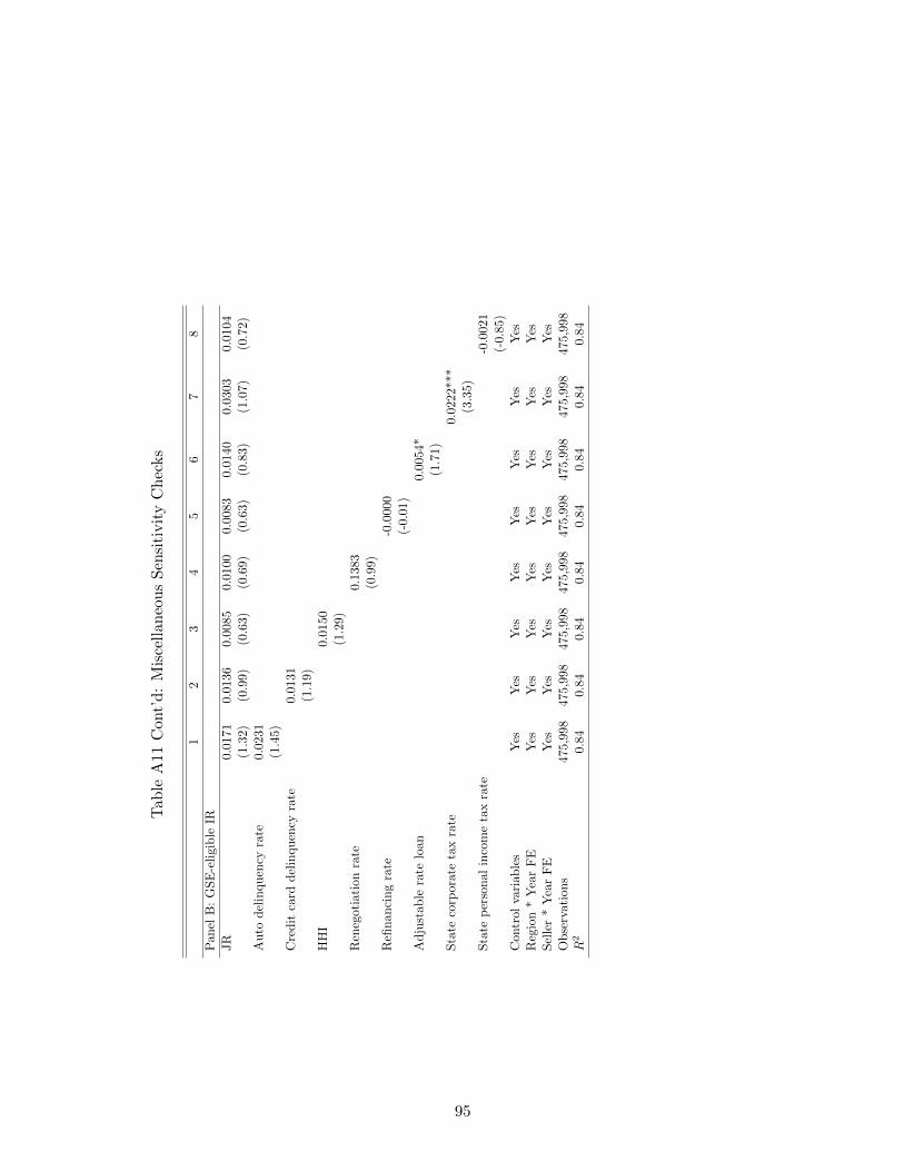
Tab
leA
11C
ont’
d:
Mis
cell
aneo
us
Sen
siti
vit
yC
hec
ks
12
34
56
78
Pan
elB
:G
SE
-eligi
ble
IR
JR
0.01
710.
0136
0.00
850.
0100
0.00
830.
0140
0.0
303
0.01
04(1
.32)
(0.9
9)(0
.63)
(0.6
9)(0
.63)
(0.8
3)(1
.07)
(0.7
2)A
uto
del
inquen
cyra
te0.0
231
(1.4
5)C
redit
card
del
inquen
cyra
te0.
0131
(1.1
9)H
HI
0.01
50(1
.29)
Ren
egot
iati
onra
te0.
1383
(0.9
9)R
efinan
cing
rate
-0.0
000
(-0.
01)
Adju
stab
lera
telo
an0.
0054
*(1
.71)
Sta
teco
rpor
ate
tax
rate
0.022
2**
*(3
.35)
Sta
tep
erso
nal
inco
me
tax
rate
-0.0
021
(-0.8
5)C
ontr
olva
riab
les
Yes
Yes
Yes
Yes
Yes
Yes
Yes
Yes
Reg
ion
*Y
ear
FE
Yes
Yes
Yes
Yes
Yes
Yes
Yes
Yes
Sel
ler
*Y
ear
FE
Yes
Yes
Yes
Yes
Yes
Yes
Yes
Yes
Obse
rvat
ions
475,
998
475,
998
475,
998
475,
998
475,
998
475,
998
475
,998
475
,998
R2
0.84
0.84
0.84
0.84
0.84
0.84
0.84
0.84
95

Tab
leA
11C
ont’
d:
Mis
cell
aneo
us
Sen
siti
vit
yC
hec
ks
12
34
56
78
Pan
elC
:N
on-G
SE
-eligi
ble
Sec
JR
0.00
720.
0071
0.00
610.
0057
0.00
630.
0125
0.0
081
0.00
59
(1.1
1)(1
.09)
(0.9
4)(0
.89)
(0.9
9)(1
.43)
(1.1
3)(0
.92)
Auto
del
inquen
cyra
te-0
.000
2(-
0.21
)C
redit
card
del
inquen
cyra
te-0
.000
6(-
0.93
)H
HI
-0.0
011
(-0.
52)
Ren
egot
iati
onra
te0.
0285
(0.4
9)R
efinan
cing
rate
-0.0
002
(-0.
49)
Adju
stab
lera
telo
an0.
0005
(0.9
8)Sta
teco
rpor
ate
tax
rate
-0.0
001
(-0.
09)
Sta
tep
erso
nal
inco
me
tax
rate
-0.0
026**
*(-
3.1
7)C
ontr
olva
riab
les
Yes
Yes
Yes
Yes
Yes
Yes
Yes
Yes
Reg
ion
*Y
ear
FE
Yes
Yes
Yes
Yes
Yes
Yes
Yes
Yes
Len
der
*Y
ear
FE
Yes
Yes
Yes
Yes
Yes
Yes
Yes
Yes
Obse
rvat
ions
74,7
9974
,799
74,7
9974
,799
74,7
9974
,799
74,7
9974
,799
R2
0.78
0.78
0.78
0.78
0.78
0.73
0.79
0.78
96

Tab
leA
11C
ont’
d:
Mis
cell
aneo
us
Sen
siti
vit
yC
hec
ks
12
34
56
78
Pan
elD
:N
on-G
SE
-eligi
ble
IR
JR
0.10
13∗∗∗
0.09
19∗∗∗
0.06
66∗∗∗
0.10
09∗∗∗
0.09
53∗∗∗
0.01
67∗∗∗
0.07
85∗∗∗
0.09
38∗∗∗
(4.3
6)(4
.04)
(2.9
0)(4
.10)
(3.9
6)(2
.82)
(3.1
1)(3
.76)
Auto
del
inquen
cyra
te0.
0185∗∗∗
(5.4
6)C
redit
card
del
inquen
cyra
te0.
0157∗∗∗
(9.0
6)H
HI
-0.0
440∗∗∗
(-5.
98)
Ren
egot
iati
onra
te-0
.122
4(-
1.51
)R
efinan
cing
rate
-0.0
036∗∗∗
(-2.
95)
Adju
stab
lera
telo
an0.
0006
(0.8
9)Sta
teco
rpor
ate
tax
rate
-0.0
230∗∗∗
(-5.7
1)Sta
tep
erso
nal
inco
me
tax
rate
-0.0
009
(-0.
37)
Con
trol
vari
able
sY
esY
esY
esY
esY
esY
esY
esY
esR
egio
n*
Yea
rF
EY
esY
esY
esY
esY
esY
esY
esY
esL
ender
*Y
ear
FE
Yes
Yes
Yes
Yes
Yes
Yes
Yes
Yes
Obse
rvat
ions
68,9
7868
,978
68,9
7868
,978
68,9
7868,
978
68,9
7868
,978
R2
0.79
0.79
0.79
0.79
0.78
0.79
0.78
0.7
9
Note
s:T
his
table
rep
ort
spara
met
ric
esti
mate
sof
equati
on
(2).
InP
anel
A(B
)th
esa
mple
conta
ins
GSE
-eligib
lelo
ans
and
the
dep
enden
tva
riable
isSec
(IR
).In
Panel
C(D
)th
esa
mple
conta
ins
non-G
SE
-eligib
lelo
ans
and
the
dep
enden
tva
riable
isSec
(IR
).T
he
contr
olva
riable
sare
the
ass
ignm
ent
vari
able
,th
eJR
-ass
ignm
ent
inte
ract
ion
vari
able
,m
inori
ty,
male
,th
eori
gin
al
LT
Vra
tio,
house
pri
cein
dex
,and
lender
sp
erca
pit
a.
Sta
ndard
erro
rsare
clust
ered
at
the
state
level
and
the
corr
esp
ondin
gt-
stati
stic
sare
rep
ort
edin
pare
nth
eses
.*,
**,
and
***
indic
ate
stati
stic
al
signifi
cance
at
the
10%
,5%
,and
1%
level
sre
spec
tivel
y.
97

Table A12: Estimates by Population and Region
1 2 3 4Sample GSE Non-GSE
Dependent variable Sec IR Sec IR
Panel A: Most populous border regions
JR 0.0171∗∗∗ -0.0156 0.0083 0.0699∗∗
(4.19) (-0.75) (1.02) (2.58)Control variables Yes Yes Yes YesRegion * Year FE Yes Yes Yes YesLender * Year FE Yes Yes Yes YesObservations 399,624 399,624 59,905 55,402R2 0.54 0.76 0.77 0.82
Panel B: Least populous borders regions
JR 0.0130∗∗ 0.0038 0.0063 0.0604∗
(2.47) (0.36) (0.53) (1.74)Control variables Yes Yes Yes YesRegion * Year FE Yes Yes Yes YesLender * Year FE Yes Yes Yes YesObservations 85,643 85,643 14,894 13,576R2 0.60 0.99 0.85 0.78
Panel C: Northeast
JR 0.0290∗∗ 0.0041 -0.0024 0.0582∗
(2.48) (0.37) (-0.11) (1.78)Control variables Yes Yes Yes YesRegion * Year FE Yes Yes Yes YesLender * Year FE Yes Yes Yes YesObservations 51,692 51,692 6,714 5,543R2 0.52 0.90 0.76 0.82
Panel D: Midwest
JR 0.0144∗∗ -0.0622 -0.0063 0.1224∗∗∗
(2.72) (-1.10) (-0.87) (4.02)Control variables Yes Yes Yes YesRegion * Year FE Yes Yes Yes YesLender * Year FE Yes Yes Yes YesObservations 194,406 194,406 26,030 23,336R2 0.56 0.92 0.76 0.84
98

Table A12 Cont’d: Estimates by Population and Region
1 2 3 4Sample GSE Non-GSE
Dependent variable Sec IR Sec IR
Panel E: West
JR 0.0470∗ -0.0081 0.0001 0.0973(1.76) (-1.05) (0.11) (1.43)
Control variables Yes Yes Yes YesRegion * Year FE Yes Yes Yes YesLender * Year FE Yes Yes Yes YesObservations 979 979 82 75R2 0.77 0.90 0.92 0.92
Panel F: South
JR 0.0111∗ 0.0185 0.0167∗ 0.0806∗∗
(1.96) (0.96) (1.95) (2.48)Control variables Yes Yes Yes YesRegion * Year FE Yes Yes Yes YesLender * Year FE Yes Yes Yes YesObservations 209,292 209,292 37,550 35,917R2 0.54 0.89 0.80 0.79
Panel G: Borders between regions
JR 0.0115∗ -0.0156 -0.0114 0.0048∗
(1.92) (-1.42) (-0.73) (1.78)Control variables Yes Yes Yes YesRegion * Year FE Yes Yes Yes YesLender * Year FE Yes Yes Yes YesObservations 29,857 29,857 4,423 4,107R2 0.64 0.87 0.88 0.77
Notes: This table presents estimates of equation (2). GSE (Non-GSE) indicates the sample includes GSE-eligible (non-GSE-eligible) loans. Sec (IR) indicates the dependent variable is the securitization dummyvariable (interest rate). The sample includes loans within 10 miles of the threshold. Panel A includesobservations from regions with above the mean population. Panel B includes observations from regionswith below the mean population. In Panel C the sample includes observations from CT, MA, ME, NH, NY,RI, and VT. In Panel D the sample includes observations from IA, IL, IN, KS, MI, MN, MO, ND, NE, OH,SD, and WI. In Panel E the sample includes observations from AZ, CO, and NM. In Panel F the sampleincludes observations from AR, KY, LA, MS, OK, TN, TX, VA, and WV. In Panel G the sample includesobservations from regions that border the accepted regions in the US (for example, between Northeasternand Southern states) AL, AR, DC, FL, GA, KY, LA, MD, MS, NC, OK, SC, TN, TX, VA, and WV.The control variables are the assignment variable, the JR-assignment interaction variable, minority, male,the original LTV ratio, house price index, and lenders per capita. Standard errors are clustered at thestate level and the corresponding t-statistics are reported in parentheses. *, **, and *** indicate statisticalsignificance at the 10%, 5%, and 1% levels respectively.
99

H: Appendix Figures
Figure A2: Mortgage Default Rates
01
23
45
67
Mor
tgag
e D
efau
lt R
ates
2000 2002 2004 2006 2008 2010 2012 2014 2016year
JR states PS states
Notes: This figure shows the mean rate of mortgage default, defined as the share of mortgages that are atleast 90 days late, in JR and PS states between 2000 and 2016. Data from 2000 to 2011 are taken fromthe NY Fed. Data from 2012 to 2016 are taken from the Consumer Finance Protection Bureau.
100

Figure A3: LATE by Border Pair (JR-PS Borders)
WV-KYMA-CT
WV-PA
TX-NM
MO-ILNE-IA
OH-MI
SD-NE
LA-AR
WV-OH
VT-NHMO-KS
TX-LA
WI-MN VA-KYVA-MDGA-FL
VT-MA
MS-LAMI-IN WV-MD
SC-GATN-KY
NH-ME
NM-AZ
OK-ARTX-OK
RI-CT
NY-MA
FL-AL
SC-NC
OK-MONM-CO
WY-SD
MO-IA
SD-MNND-MN
ND-MT
WI-MI
NE-KS
MN-IA
MD-DC
-.1-.0
50
.05
.1.1
5G
SE s
ecur
itiza
tion
Significant Not significant
Panel A: GSE securitization
WV-PA
NH-ME
FL-ALSC-NC
OK-MO
NM-COWV-KY MA-CTWY-SD
MO-IA
TX-NM
MO-IL
NE-IA
OH-MI LA-ARWV-OH
VT-NHMO-KS
SD-MN TX-LA
ND-MN
WI-MN VA-KY VA-MDGA-FLVT-MA
ND-MT
MS-LAMI-IN WV-MDWI-MI
SC-GATN-KY
NE-KS
NM-AZ
OK-ARTX-OK
RI-CT
MN-IA
MD-DC
NY-MA
-.4-.2
0.2
.4N
on-G
SE s
ecur
itiza
tion
Significant Not significant
Panel C: Non-GSE securitization
TX-NM
TX-LA WV-MD
WI-MI
SC-GA
TX-OK
RI-CT
MD-DCFL-AL
SC-NC
OK-MO
NM-CO
WV-KY
MA-CT
WY-SD
WV-PA
MO-IA
MO-IL
NE-IA
OH-MI
SD-NE
LA-ARWV-OH
VT-NH
MO-KS
SD-MN
ND-MN
WI-MN
VA-KY
VA-MD
GA-FL
VT-MA
ND-MT
MS-LA
MI-IN
TN-KY
NE-KS
NH-ME
NM-AZ
OK-AR
MN-IA
NY-MA
-.3-.2
5-.2
-.15
-.1-.0
50
.05
.1.1
5.2
.25
.3G
SE In
tere
st ra
tes
Significant Not significant
Panel B: GSE interest rates
WV-PATX-NMMO-ILNE-IAOH-MILA-ARWV-OHVT-NH TX-LA VA-KYVA-MDGA-FL MS-LAMI-INWV-MDTN-KYNH-ME
OK-ARTX-OKRI-CT
MN-IA
MD-DC
NY-MA
FL-AL
SC-NCOK-MONM-COWV-KYMA-CTWY-SDMO-IA SD-NEMO-KSSD-MNND-MNWI-MN VT-MAND-MTWI-MISC-GA
NE-KSNM-AZ
-.50
.51
1.5
2N
on-G
SE in
tere
st ra
tes
Significant Not significant
Panel D: Non-GSE interest rates
Notes: This figure reports estimates of β in equation (2) for each border pair between a JR and PS state. Toobviate small sample problems, we restrict the sample to border pairs that have at least 100 observations.For example, we restrict the sample to loans within 10 miles of the border between Vermont (JR) andMassachusetts (PS). We then estimate equation (2), save the coefficient on the JR dummy variable, β,and report β for each border-pair in the data set. Panel A reports β using GSE-eligible securitization asthe dependent variable. Panel B reports β using GSE-eligible interest rates as the dependent variable.Panel C reports β using non-GSE-eligible securitization as the dependent variable. Panel D reports βusing non-GSE-eligible interest rates as the dependent variable. Red circles indicate that β is statisticallysignificant at least at the 5% level. Blue triangles denote that β is statistically insignificant.
101

Figure A4: LATE by Border Pair (JR-JR Borders)
IL-IA
OH-IN
IN-IL PA-NJ
PA-MDWI-IL
OH-NYPA-NY
VT-NY
NY-CT
SD-IA
KY-IN
NY-NJ
NJ-DEPA-OH MD-DE
KY-IL
OK-KSOH-KY
-.2-.1
5-.1
-.05
0.0
5.1
.15
.2G
SE s
ecur
itiza
tion
Significant Not Significant
Panel A: GSE securitization
IL-IA
PA-OH
MD-DEOH-NYKY-IN
PA-MDWI-ILOH-KY
KY-ILNY-NJ
PA-NJNY-CT
IN-ILSD-IA PA-NYOK-KS
VT-NYOH-IN
NJ-DE
-.2-.1
0.1
.2N
on-G
SE s
ecur
itiza
tion
Significant Not significant
Panel C: Non-GSE securitization
IN-ILPA-NJ
PA-MD
WI-IL
IL-IA
OH-NYPA-NY
VT-NY
NY-CT
OH-IN
SD-IA
KY-IN
NY-NJ
NJ-DE
PA-OHMD-DE
KY-IL
OK-KS
OH-KY
-.3-.2
-.10
.1G
SE In
tere
st R
ates
Significant Not Significant
Panel B: GSE interest rates
SD-IA
IL-IA
PA-OH
MD-DE
OH-NY
KY-IN
PA-MDWI-IL
OH-KY
KY-IL
NY-NJ
PA-NJ
NY-CT
IN-IL
PA-NY
OK-KS
VT-NYOH-IN
NJ-DE
-1-.5
0.5
1N
on-G
SE in
tere
st ra
tes
Significant Not significant
Panel D: Non-GSE interest rates
Notes: This figure reports estimates of β in equation (5) for each border pair between a JR and JRstate. To obviate small sample problems, we restrict the sample to border pairs that have at least 100observations. We first restrict the sample to loans within 10 miles of the border between two states thatboth use JR law (for example, Kentucky and Indiana). We then randomly assign one state to placebotreatment status (for example, Kentucky) and one state to placebo control status (for example, Indiana).We then estimate equation (5), save the coefficient on the Placebo dummy variable, β, and report β foreach border-pair in the data set. Panel A reports β using GSE-eligible securitization as the dependentvariable. Panel B reports β using GSE-eligible interest rates as the dependent variable. Panel C reports βusing non-GSE-eligible securitization as the dependent variable. Panel D reports β using non-GSE-eligibleinterest rates as the dependent variable. Red circles indicate that β is statistically significant at least atthe 5% level. Blue triangles denote that β is statistically insignificant.
102

Figure A5: LATE by Border Pair (PS-PS Borders)
WA-OR
NV-CA
OR-ID
NH-MA
NV-AZVA-DC
TX-ARRI-MA
MT-ID
TN-ARTN-MS
UT-AZ
MO-AR
TN-GA
WA-ID
TN-MO
NC-GA
TN-ALVA-NC
MS-AR
-.2-.1
0.1
.2G
SE S
ecur
itiza
tion
Significant Not significant
Panel A: GSE securitization
VA-DC
OR-ID
NH-MA
NV-AZ
TX-ARRI-MA
MT-ID
TN-AR
TN-MS
WA-OR
UT-AZMO-AR TN-GA
WA-ID
TN-MO
NC-GA
NV-CA
TN-AL
VA-NC
MS-AR
-.3-.2
-.10
.1.2
Non
-GSE
sec
uriti
zatio
n
Significant Not significant
Panel C: Non-GSE securitization
WA-ORVA-NC
OR-ID
NH-MANV-AZ
VA-DC
TX-AR
RI-MA
MT-ID TN-ARTN-MSUT-AZ
MO-AR
TN-GAWA-ID
TN-MO
NC-GANV-CA
TN-ALMS-AR
-.2-.1
0.1
.2G
SE in
tere
st ra
tes
Significant Not Significant
Panel B: GSE interest rates
VA-DC
OR-ID
NH-MA
NV-AZTX-ARRI-MA MT-ID
TN-ARTN-MS WA-OR
UT-AZ
MO-ARTN-GA
WA-IDTN-MO NC-GA
NV-CA TN-ALVA-NC
MS-AR
-2-1
.5-1
-.50
.51
1.5
2N
on-G
SE in
tere
st ra
tes
Significant Not Significant
Non-GSE Interest rates
Notes: This figure reports estimates of β in equation (5) for each border pair between a PS and PS state. Toobviate small sample problems, we restrict the sample to border pairs that have at least 100 observations.We first restrict the sample to loans within 10 miles of the border between two states that both use JRlaw (for example, Arizona and Utah). We then randomly assign one state to placebo treatment status(for example, Arizona) and one state to placebo control status (for example, Utah). We then estimateequation (5), save the coefficient on the Placebo dummy variable, β, and report β for each border-pairin the data set. Panel A reports the LATE using GSE-eligible securitization as the dependent variable.Panel B reports the LATE using GSE-eligible interest rates as the dependent variable. Panel C reportsthe LATE using non-GSE-eligible securitization as the dependent variable. Panel D reports the LATEusing non-GSE-eligible interest rates as the dependent variable. Red circles indicate that β is statisticallysignificant at least at the 5% level. Blue triangles denote that β is statistically insignificant.
Online Appendix References
Fox, J. (2015) ’The Future of Foreclosure Law in the Wake of the Great Housing Crisis of
2007-2014’, Washburn Law Journal, 54: 489-526.
103